Nonlocal second-order geometric equations arising in tomographic reconstruction

Nonlinear Analysis 70 (2009) 1746–1762www.elsevier.com/locate/na

Nonlocal second-order geometric equations arising intomographic reconstruction

Ali Srour∗

Laboratoire de Mathematiques et Physique Theorique, Universite Francois-Rabelais Tours, Federation Denis Poisson -UMR CNRS 6083,Parc de Grandmont, 37200 Tours, France

Laboratoire de Mathematiques et Applications Physique Mathematique d’Orleans, 45067 Orleans Cedex 2, France

Received 12 March 2007; accepted 22 February 2008

Abstract

In this paper, we study new nonlocal geometric equations which are related to tomographic reconstruction when using thelevel-set approach. We treat two additional difficulties which make the work original. On one hand, the level lines do not evolvealong normal directions and the nonlocal term is not of “convolution type”. On the other hand, the speed is not necessarily boundedcompared to the nonlocal term. We prove an existence and uniqueness result for our equation.c© 2008 Elsevier Ltd. All rights reserved.

Keywords: Nonlocal Hamilton–Jacobi equations; Tomographic reconstruction; Nonlocal front propagation; Level-set approach; Viscosity solutions

In this paper, we study a fully nonlinear parabolic equation with nonlocal term, more precisely,∂u

∂t(x, t) = F(x, t, Du, D2u, K k,+

x,t,u) in RN× [0, T ] ,

u(x, 0) = u0(x) in RN× 0 ,

(1)

where N ≥ 1 is an integer, T > 0. The unknown function is u : RN×[0, T ] −→ R, Du and D2u denote respectively

the gradient and the Hessian of u with respect to the space variable, u0: RN−→ R is the given initial data, and K k,+

x,t,udenotes the nonlocal term given for some integer k ≤ N by

K k,+x,t,u = [u]

+x,t ∩ Ak

x

where

[u]+x,t =

y ∈ RN: u(y, t) ≥ u(x, t)

and

Akx =

y = (y1, . . . , yk, yk+1, . . . , yN ) ∈ RN

: πk(y) = πk(x)

∗ Corresponding address: Laboratoire de Mathematiques et Physique Theorique, Universite Francois-Rabelais Tours, Federation Denis Poisson-UMR CNRS 6083, Parc de Grandmont, 37200 Tours, France. Fax: +33 02 47 36 70 68.

E-mail address: [email protected].

0362-546X/$ - see front matter c© 2008 Elsevier Ltd. All rights reserved.doi:10.1016/j.na.2008.02.077

http://www.elsevier.com/locate/na

mailto:[email protected]

http://dx.doi.org/10.1016/j.na.2008.02.077

A. Srour / Nonlinear Analysis 70 (2009) 1746–1762 1747

where πk denotes the projection function from RN into Rk defined by

πk(x) = (x1, . . . , xk)

for all x = (x1, . . . , xk, xk+1, . . . , xN ). In the same manner

K k,−x,t,u = [u]

−x,t ∩ Ak

x

where

[u]−x,t =

y ∈ RN: u(y, t) > u(x, t)

.

The nonlinearity F is a continuous function from RN×R×RN

\ 0 ×SN ×BN−k into R, where SN is the set ofreal symmetric N × N matrices and BN−k is the set of equivalence classes of all subsets of RN−k with respect to therelation A ∼ B if L N−k(A∆B) = 0, where L N−k is the Lebesgue measure on RN−k .

We consider BN−k with a topology that comes from the metric

d(A, B) =∞∑

n=0

L N−k ((A∆B) ∩ B(0, n))

2n L N−k(B(0, n)),

where B(0, n) denotes the ball in RN−k of center 0 and radius n. With this topology a sequence (K kn )n≥1 in BN−k

converges to K k∈ BN−k if and only if 1K k

nconverges to 1K k in L1

loc(RN−k).

Here, we give in dimension 2 an example of an equation which is related to tomographic reconstruction when usingactive curves and the level-set approach [12,7] and which has the same type of nonlocal term as Eq. (1). The modelcase that we have in mind is

∂u

∂t(x, t) = C(x, t)

(∫K 1,+

x,t,u

g(z)dz

)|Du| + Trace

[(I −

Du ⊗ Du

|Du|2

)D2u

],

u(x, 0) = u0(x) in R2× 0 ,

(2)

where x = (x1, x2), g is a positive function and g ∈ L1(R), C is a Lipschitz continuous function, and K 1,+x,t,u is given

by

K 1,+x,t,u =

y = (y1, y2) ∈ R2

: u(y, t) ≥ u(x, t)∩ y1 = x1

= [u]+x,t ∩ A1x .

We recall that the level-set approach was first introduced by Osher and Sethian [13] for numerical computations. Itwas then developed from a theoretical point of view by Evans and Spruck [10] for motion by mean curvature and byChen, Giga and Goto [8] for general normal velocities. We also refer the reader to Barles, Soner and Souganidis [3]and Souganidis [15,16] for different presentations and other results on the level-set approach.

In [14], Slepcev studied the motion of fronts in bounded domains with normal velocities which can depend on thenonlocal terms, in addition to the curvature, the normal direction and the location of the front. In fact, the velocitiesdepend on the nonlocal terms if the velocities at any point of the front depend on the set that the front encloses.Depending on the velocities, the motion of the front can be described by the partial differential equation

∂u

∂t(x, t) = F(x, t, Du(x, t), D2u(x, t), [u]+x,t ) in O × [0, T ] (3)

with the Neumann boundary conditions ∂u/∂γ = 0 on ∂O × [0, T ] and u(x, 0) = u0(x), where O is a boundeddomain in RN. Slepcev proved an existence and uniqueness result for this equation, using the viscosity solution.

In [2], Barles, Cardaliaguet, Ley and Monneau studied the first-order nonlocal equation∂u

∂t(x, t) =

(C0(., t) ∗ 1

[u]+x,t(x, t)+ C1(x, t)

)|Du| in RN

× [0, T ] ,

u(x, 0) = u0(x) in RN× 0 .

(4)

1748 A. Srour / Nonlinear Analysis 70 (2009) 1746–1762

This equation appears when modelling dislocations in crystals using the level-set approach. The ∗ denotes theconvolution in space, C0 and C1 are two functions on which we have some conditions. They proved an existence anduniqueness result for this equation in both cases where C0 is a positive and a negative function, C0(., t) ∈ L1(RN ) forall t ∈ [0, T ], and C0,C1 are two Lipschitz continuous functions.

Now a question emerges: what are the differences between the Eqs. (1) and (2) and (3) and (4)? We consider thecase N = 2 to explain, for example, the differences between the Eq. (2) and (4). In (4), for any (x, t) ∈ R2

× [0, T ]where x = (x1, x2), the nonlocal term is given by

[u]+x,t =

y ∈ R2: u(y, t) ≥ u(x, t)

.

and we integrate on a subset of R2. In our Eq. (2), the new nonlocal term is given for any (x, t) ∈ R2× [0, T ] by

K 1,+x,t,u =

y = (y1, y2) ∈ R2

: u(y, t) ≥ u(x, t)∩ y1 = x1 ,

and we integrate in (2) over a straight line, i.e. the first variable is always fixed. We remark that the technique usedin [2,14] cannot be applied in the case of this new nonlocal term. Therefore, we change the dependence in Du, inorder to be able to prove a uniqueness and existence result for our Eq. (1) using techniques inspired by [2,14].

Moreover, contrary to the cases studied in [2,14], in the initial compact front, our approach allows an unboundeddependence of volume in our Eq. (1) (see (H5-1) and (H6-1)).

Let us now explain how this paper is organized: In Section 1, we present our problem and we recall the definitionof viscosity solutions. In Section 2, we prove a uniqueness result for our equation with compact fronts. In Section 3we show a uniqueness result for noncompact fronts. In Section 4, we prove an existence result for compact andnoncompact fronts. Finally, we give, in the Appendix, the proof of the stability result for Eq. (1).

1. Presentation of our problem

Tomography processes are widely studied by many authors. Most of the cases studied concern image restorationfrom a lot of projected data. In [17], M. Somekh addresses the problem of reconstruction of an image from twopairs of its orthogonal projections. The paper by Dinten, Bruandet, Peyrin, Amadieu and Barlaud [7] addressestomographic reconstruction of binary objects from a small number of noisy projections in applications where theglobal dose remains constant with an increase or a decrease of the number of projections. Here we are interested inthe reconstruction method of [12], where the authors consider a single view of tomographic reconstruction for radiallysymmetric objects and binary image. They formulate the problem as a front propagation which consists in evolvingthe contour of the noisy image (initial front), with a selected normal velocity, so that it converges toward the contourof the initial object. This evolution is described by the level-set approach which leads to a nonlocal equation

∂u

∂t(x, t) = C(x, t)

(∫z∈R:u(x1,z,t)≥0

g(z)dz

)|Du| + Trace

[(I −

Du ⊗ Du

|Du|2

)D2u

],

u(x, 0) = u0(x) in R2× 0 ,

(5)

where x = (x1, x2) ∈ R2, g is a positive function and g ∈ L1(R). The second term on the right hand side of (5) is themean curvature. This term was studied in [10] where it was used to regularize the evolution of the initial front withnormal velocity.

First, for this equation, even the existence of solutions is not known. The major difficulty is due to the factthat the function C has negative value. From a geometrical point of view, the front propagation does not satisfyany monotonicity property (preservation of inclusion). The monotonicity property of the front propagation problemis almost equivalent to the comparison principle theorem for viscosity solutions and can be expressed in thefollowing way: if (Ω1

t )t≥0, (Ω2t )t≥0 are two families of open subsets evolving with the same normal velocity then, if

(Ω10 ) ⊂ (Ω

20 ), one has

(Ω1t ) ⊂ (Ω

2t ), ∀t ≥ 0.

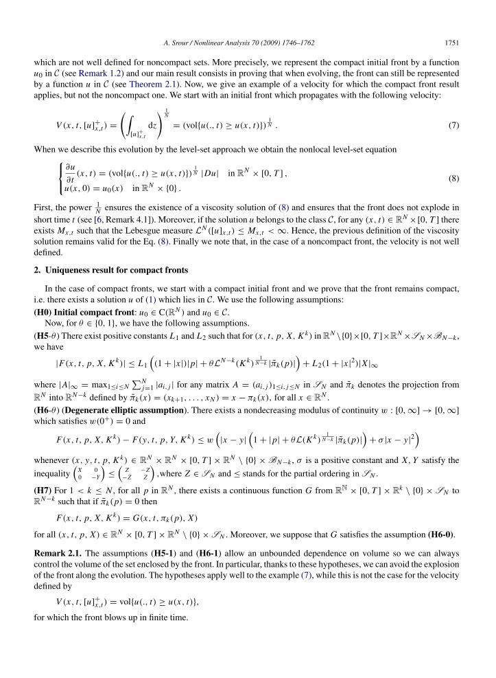
Secondly, since x1 is fixed in (5), a discontinuity appears in the normal speed of propagation. To see this problemof continuity it is enough to start with a rectangular initial front whose sides are parallel to the coordinate axes and


Fig. 1. Rectangular initial front.

this rectangle can be represented as a level-set zero of a function u from R2× [0, T ] to R, i.e. u = 0 on the sides,

u > 0 inside the rectangle and u < 0 outside (see Fig. 1). Suppose that this front evolves with a normal simplifiedvelocity given by

V (x, y, t) =∫z∈R:u(x,z,t)≥0

dz,

where (x, y) ∈ R2, t ∈ [0, T ]. Now, we consider the points (l, y, t) where l is the width of the rectangle and 2lis its length. It is easy to prove that the velocity at these points is l, but if we move horizontally to (l + ε, y), thevelocity becomes V (l + ε, y, t) = 0. So, we conclude that moving horizontally causes a jump in the velocity. Now,because of the new form of the nonlocal term, the classical technique for proving the uniqueness and existence of aviscosity solution ceases to hold which makes it interesting, at least from a theoretical point of view, to study this kindof problem. In order to be able to solve the Eq. (5) by using the arguments of the classical technique, we make twochanges to our original Eq. (5). First, we change the sign of C in order to preserve the inclusion property with theprospect of dealing with the case C ≤ 0 in a future work. Secondly, in our present work, we change the dependencewith respect to the Du variable. More precisely, instead of evolving in the normal direction, we will evolve in thevertical direction. In this case, the vertical sides of the rectangle remain fixed, whereas the two horizontal sides movein opposite senses along the vertical direction. In addition, a numerical study would be very important for this type ofpropagation.

Moreover, as was remarked by Slepcev [14], in the level-set approach, all level-sets of the solution u should havethe same type of normal velocity. A nonlocal term using [u]+x,t instead of u(., t) ≥ 0 is more appropriate. After thesemodifications, the Eq. (5) becomes

∂u

∂t(x, t) = C(x, t)

(∫K 1,+

x,t,u

g(z)dz

) ∣∣∣∣ ∂u

∂x2

∣∣∣∣+ Trace[(

I −Du ⊗ Du

|Du|2

)D2u

],

u(x, 0) = u0(x) in R2× 0 ,

(6)

and we will prove in Section 3 uniqueness and existence of a viscosity solution for (6).We now list the basic requirements on F . The main assumptions, introduced because of the presence of the nonlocal

term, are the monotonicity with respect to set inclusion and the continuity of F with respect to the topology on BN−kwhich is defined in the introduction.

(H1) F is continuous from RN× [0, T ] × RN

\ 0 ×SN ×BN−k into R.(H2) For all (x, t, K k, Lk) ∈ RN

× [0, T ] ×BN−k ×BN−k , we have

−∞ < F?(x, t, 0, O, K k) = F?(x, t, 0, O, Lk) < +∞.

Here F? denotes the upper semicontinuous envelope of F , while F? is the lower semicontinuous envelope of F . Werecall that if f : S → R where S is a subset of some RN , the upper- and lower semicontinuous envelopes f ? and f?of f are given by

f ?(y) = lim supz→y

f (z) and f?(y) = lim infz→y

f (z).


(H3)(Monotonicity assumption). F is nondecreasing in its set argument, i.e., for any K k , Lk in BN−k such thatK k⊂ Lk , we have

F(x, t, p, X, K k) ≤ F(x, t, p, X, Lk)

for any X in SN , and for any (x, t, p) in RN× [0, T ] × RN

\ 0.

(H4) F is geometric: for any λ > 0, µ ∈ R, we have

F(x, t, λp, λX + µp ⊗ p, K k) = λF(x, t, p, X, K k)

for all (x, t, p, X, K k) ∈ RN× [0, T ] × RN

\ 0 ×SN ×BN−k .

Definition 1.1 (Slepcev [14]). An upper semicontinuous function u : RN× [0, T ] −→ R is a viscosity subsolution

of (1) if, for any φ ∈ C2(RN× [0, T ]), for any maximum point (x, t) of u − φ, if t > 0 then

∂φ

∂t(x, t) ≤ F?(x, t, Dφ(x, t), D2φ(x, t), K k,+

x,t,u)

and u(x, 0) ≤ u0(x) if t = 0. A lower semicontinuous function u: RN× [0, T ] −→ R is a viscosity supersolution of

(1) if, for any φ ∈ C2(RN× [0, T ]), for any minimum point (x, t) of u − φ, if t > 0 then

∂φ

∂t(x, t) ≥ F?(x, t, Dφ(x, t), D2φ(x, t), K k,−

x,t,u)

and u(x, 0) ≥ u0(x) if t = 0.A function is a viscosity solution of (1) if it is both a subsolution and supersolution of (1).

Remark 1.1. In the definition of a subsolution and a supersolution, “test sets” were chosen differently. This is amajor point when viscosity solutions are to be extended to nonlocal, geometric parabolic equations. If “≥” were usedinstead of “>” in the definition of supersolutions, existence results, among other things, would no longer hold. Formore information, we refer the reader to the arguments given by Slepcev in [14, Definition 2.1]. For convenience, wegive an alternative proof for these arguments in the Appendix.

For in the initial compact front we will seek the solutions of our equation (the solution of which represents the frontvia its zero level-set) using functions in the class C given by the following definition.

Definition 1.2. A function u : RN× [0, T ] → R is in the class C if −1 < u(x, t) ≤ 1 and infx∈RN u(x, t) =

lim|x |→+∞ u(x, t) = −1 for all x in RN and uniformly with respect to t ∈ [0, T ].

Remark 1.2. All continuous functions in C are uniformly continuous bounded functions and any compact front canbe represented as a level-set zero of a function in C. Indeed, let E ⊂ RN be a bounded open set and Γ0 = ∂E be theinitial compact front. This front is represented by the signed function defined by

ds∂E (x) = d(x,RN

\ E)− d(x, E),

where d(x, E) denotes the distance function, to E . It is easy to check that ds∂E (x) > 0 if x ∈ E , ds

∂E (x) < 0 ifx ∈ RN

\ E , and ds∂E (x) = 0 if and only if x ∈ Γ0. Moreover ds

∂E is Lipschitz continuous with constant 1. Now,we consider the function f (x) = 2 arctan(ds

∂E (x))/π and we use the properties of the arctan function to prove thatf (x) > −1 for all x ∈ RN and f (x) tends to −1 as x tends to ∞. Then, f ∈ C and the initial compact frontΓ0 is represented by f . A typical example of a function which belongs to this class is g(x, t) = e−At

1+|x |2− 1 where

(x, t) ∈ RN× [0, T ] and A is a positive constant.

Now, another question emerges: for what reason do we use the class C for subsolutions and supersolutions in thecompact front case? The nonlocal velocity at any point of the front depends on the set that the front encloses. In somecases, the velocity could not be defined, for instance when the volume of the set is infinite (see the example of the“volume velocity” below). With this kind of velocity, we always start with a compact initial front and our goal is toshow that the front remains compact along the evolution. From a geometrical point of view, this kind of well definedvelocity does not grow the sets too quickly. In this paper, we use the class C to define the evolution with velocities


which are not well defined for noncompact sets. More precisely, we represent the compact initial front by a functionu0 in C (see Remark 1.2) and our main result consists in proving that when evolving, the front can still be representedby a function u in C (see Theorem 2.1). Now, we give an example of a velocity for which the compact front resultapplies, but not the noncompact one. We start with an initial front which propagates with the following velocity:

V (x, t, [u]+x,t ) =

(∫[u]+x,t

dz

) 1N

= (volu(., t) ≥ u(x, t))1N . (7)

When we describe this evolution by the level-set approach we obtain the nonlocal level-set equation∂u

∂t(x, t) = (volu(., t) ≥ u(x, t))

1N |Du| in RN

× [0, T ] ,

u(x, 0) = u0(x) in RN× 0 .

(8)

First, the power 1N ensures the existence of a viscosity solution of (8) and ensures that the front does not explode in

short time t (see [6, Remark 4.1]). Moreover, if the solution u belongs to the class C, for any (x, t) ∈ RN×[0, T ] there

exists Mx,t such that the Lebesgue measure L N ([u]x,t ) ≤ Mx,t < ∞. Hence, the previous definition of the viscositysolution remains valid for the Eq. (8). Finally we note that, in the case of a noncompact front, the velocity is not welldefined.

2. Uniqueness result for compact fronts

In the case of compact fronts, we start with a compact initial front and we prove that the front remains compact,i.e. there exists a solution u of (1) which lies in C. We use the following assumptions:(H0) Initial compact front: u0 ∈ C(RN ) and u0 ∈ C.

Now, for θ ∈ 0, 1, we have the following assumptions.(H5-θ ) There exist positive constants L1 and L2 such that for (x, t, p, X, K k) in RN

\0×[0, T ]×RN×SN×BN−k ,

we have

|F(x, t, p, X, K k)| ≤ L1

((1+ |x |)|p| + θL N−k(K k)

1N−k |πk(p)|

)+ L2(1+ |x |2)|X |∞

where |A|∞ = max1≤i≤N∑N

j=1 |ai, j | for any matrix A = (ai, j )1≤i, j≤N in SN and πk denotes the projection fromRN into RN−k defined by πk(x) = (xk+1, . . . , xN ) = x − πk(x), for all x ∈ RN .(H6-θ ) (Degenerate elliptic assumption). There exists a nondecreasing modulus of continuity w : [0,∞] → [0,∞]which satisfies w(0+) = 0 and

F(x, t, p, X, K k)− F(y, t, p, Y, K k) ≤ w(|x − y|

(1+ |p| + θL(K k)

1N−k |πk(p)|

)+ σ |x − y|2

)whenever (x, y, t, p, K k) ∈ RN

× RN× [0, T ] × RN

\ 0 ×BN−k , σ is a positive constant and X, Y satisfy the

inequality(

X 00 −Y

)≤

(Z −Z−Z Z

),where Z ∈ SN and ≤ stands for the partial ordering in SN .

(H7) For 1 < k ≤ N , for all p in RN , there exists a continuous function G from RN × [0, T ] × Rk\ 0 ×SN to

RN−k such that if πk(p) = 0 then

F(x, t, p, X, K k) = G(x, t, πk(p), X)

for all (x, t, p, X) ∈ RN× [0, T ] × RN

\ 0 ×SN . Moreover, we suppose that G satisfies the assumption (H6-0).

Remark 2.1. The assumptions (H5-1) and (H6-1) allow an unbounded dependence on volume so we can alwayscontrol the volume of the set enclosed by the front. In particular, thanks to these hypotheses, we can avoid the explosionof the front along the evolution. The hypotheses apply well to the example (7), while this is not the case for the velocitydefined by

V (x, t, [u]+x,t ) = volu(., t) ≥ u(x, t),

for which the front blows up in finite time.


Remark 2.2. The assumption (H7) represents well the modification of the Du dependence. From a technical point ofview, this modification, as noted in the presentation of our problem, permits us to prove the uniqueness of a viscositysolution for our Eq. (1).

Theorem 2.1 (Comparison Principle). Assume (H0), (H1), (H2), (H3), (H4), (H5-1), (H6-1), (H7). Let u ∈ C(resp. v ∈ C) be a bounded upper semicontinuous subsolution of (1) (resp. bounded lower semicontinuoussupersolution of (1)); then u ≤ v in RN

× [0, T ].

Corollary 2.1. Under the assumptions of Theorem 2.1, there exists a unique viscosity solution u ∈ C of (1).

The proof of this Corollary is postponed to the Appendix.

Proof of Theorem 2.1. 1. The test function. We argue by contradiction assuming that there exists (x, t) ∈ RN×[0, T ]

such that

u(x, t)− v(x, t) = M > 0.

Since u and v are bounded, the following supremum:

Mε,η = sup(x,y,t)∈(RN )2×[0,T ]

u(x, t)− v(y, t)−

N∑i=0

|xi − yi |4

4ε4 − ηt

(9)

is finite for any ε, η > 0. We choose η small enough that

Mε,η ≥M

2> 0. (10)

Since u, v ∈ C, we have

lim|x |→+∞

[u(x, t)− v(x, t)] = 0

uniformly with respect to t ∈ [0, T ]. Therefore from (10), the supremum in (9) is achieved at a point (x, y, t),

Mε,η = u(x, t)− v(y, t)−N∑

i=1

|xi − yi |4

4ε4 − ηt . (11)

Actually x, y and t depend on ε, η, but we omit this dependence in the notation for simplicity.2. Viscosity inequalities when t > 0. From the fundamental result of the ‘User’s guide to viscosity solutions’ [9,

Theorem 8.3], for every ρ > 0, we get a1, a2 ∈ R and X , Y ∈ SN such that

(a1, p, X) ∈ P 2,+u(x, t), (a2, p, Y ) ∈ P 2,−v(y, t)

and

−1ρ

(I 00 I

)≤

(X 00 −Y

)≤

(Z + ρZ2

−(Z + ρZ2)

−(Z + ρZ2) Z + ρZ2

)a1 − a2 = η,

for Z = D2ϕ(x − y), where ϕ(x − y) =∑N

i=0|xi−yi |

4

4ε4 , I is the identity matrix and

p =

(|x1 − y1|

2(x1 − y1)

ε4 , . . . ,|xN − yN |

2(xN − yN )

ε4

).

Writing that u is a subsolution and v a supersolution of (1), we have

η ≤ F?(x, t, p, X , K k,+x,t,u)− F?(y, t, p, Y , K k,−

y,t,v). (12)


Remark 2.3. The reader should note a difficulty in applying [9, Theorem 8.3] here. Indeed, one should double thetime variable to prove [9, Theorem 8.3]. It is not straightforward here because of the presence of the nonlocal term.This problem is solved by using the stability result provided in [14]. However, we give another proof of the stabilityin the Appendix.

3. Comparison of the nonlocal terms. From the definition of Mε,η, for all (x, y) ∈ RN× RN , we have

u(x, t)− v(y, t)−∑N

i=1|xi−yi |

4

4ε4 ≤ u(x, t)− v(y, t)−∑N

i=1|xi−yi |

4

4ε4 .Taking x = (πk(x), z) and y = (πk(y), z), for any z ∈ RN−k , we have

u(πk(x), z, t)− v(πk(y), z, t)−k∑

i=1

|xi − yi |4

4ε4 ≤ u(x, t)− v(y, t)−N∑

i=1

|xi − yi |4

4ε4 ,

and thus we obtain

u(πk(x), z, t)− u(x, t) ≤ v(πk(y), z, t)− v(y, t)−N∑

i=k+1

|xi − yi |4

4ε4 . (13)

4. Upper bound for the volume K k,+x,t,u and conclusion.

Since u, v ∈ C and by (10) and (11), x and y remain bounded independently of ε and η. Using v ∈ C, we write

limε,η→0

v(y, t) > −1,

and then, there exists a positive constant µ, independent of ε and η, such that v(y, t) ≥ −1+ µ. Then

K k,+y,t,v ⊂ z ∈ RN−k

: v(πk(y), z, t) ≥ −1+ µ ⊂ B(0, R)

where R is a positive constant independent of ε and η. By the inequality (13), if u(πk(x), z, t)− u(x, t) ≥ 0, we havev(πk(y), z, t)− v(y, t) ≥ 0, and then

K k,+x,t,u ⊂ K k,+

y,t,v ⊂ B(0, R). (14)

We distinguish two cases:First case: xi = yi for all k < i ≤ N . In this case we have

p =

(|x1 − y1|

2(x1 − y1)

ε4 , . . . ,|xk − yk |

2(xk − yk)

ε4 , 0, . . . , 0).

In other words, πk( p) = 0. First, if xi = yi for any 1 ≤ i ≤ k then p = 0. But, by [9, Theorem 3.2], and [5, Lemma2.4.3], there exist X ′, Y ′ ∈ S N such that

X ≤ X ′ ≤ Y ′ ≤ Y ,

with X ′ = Y ′ = 0 when p = 0. Taking advantage of the ellipticity of F? and F?, we get from (12)

η ≤ F?(x, t, 0, O, K k,+x,t,u)− F?(x, t, 0, O, K k,−

y,t,v).

Assumption (H2) implies that

η ≤ 0,

which is a contradiction since η > 0.Therefore, there exists 1 ≤ i0 ≤ k such that xi0 6= yi0 and p 6= 0. Using (H7) and the viscosity inequality in (12),

we get

η ≤ G(x, t, πk( p), X)− G(y, t, πk( p), Y ).

By (H7), G satisfies the assumption (H6-0) and then

η ≤ w(|x − y| (1+ |πk( p)|)+ σ |x − y|2

)≤ w

(|x − y| (1+ | p|)+ σ |x − y|2

). (15)


Since | p| < |x−y|3

4ε4 , then |x − y|| p| ≤ |x−y|4

4ε4 . From this estimate, the inequality in (15) becomes

η ≤ w

(|x − y| +

|x − y|4

4ε4 + σ |x − y|2). (16)

Classical arguments [9, Remark 3.8] show that |x − y| and the penalization term∑N

i=1|xi−yi |

4

4ε4 tends to 0 if ε tends to

0, and then |x−y|4

4ε4 tends to 0 if ε tends to zero. Finally we let ε tend to 0 in (15), to obtain η ≤ 0 which is absurd.

Second case: There exists i0 such that k < i0 ≤ N and xi0 6= yi0 . In this case, for all z ∈ RN−k , we have from (13)

u(πk(x), z, t)− u(x, t) ≤ v(πk(y), z, t)− v(y, t)−|xi0 − yi0 |

4

4ε4

< v(πk(y), z, t)− v(y, t).

and therefore

K k,+x,t,u ⊂ K k,−

y,t,v. (17)

Since p 6= 0 in this case, the viscosity inequality in (12) becomes

η ≤ F(x, t, p, X , K k,+x,t,u)− F(y, t, p, Y , K k,−

x,t,v).

From (H3) and (17), we get

η ≤ F(x, t, p, X , K k,+x,t,u)− F(y, t, p, Y , K k,+

x,t,u).

We use the assumption (H6-1) to write

η ≤ w(|x − y|

(1+ | p| + L N−k(K k,+

x,t,u)1

N−k |πk( p)| + σ |x − y|2)). (18)

Now, using the estimate in (14), we have

L N−k(K k,+x,t,u)

1N−k ≤ L N−k(B(0, R))

1N−k ≤ CN−k R

where CN−k = L N−k (BN−k (0, 1))1

N−k , and R is independent of ε. Then

η ≤ w(|x − y| (1+ | p| + CN−k R|πk( p)|)+ σ |x − y|2

)≤ w

(|x − y| +

|x − y|4

4ε4 + CN−k R|x − y|4

4ε4 + σ |x − y|2). (19)

Since we know that |x−y|4

4ε4 tends to 0 as ε tends to 0, therefore |x − y| converges to 0 as ε goes to 0 and the aboveinequality (19) implies that η ≤ 0 which is a contradiction since η > 0.

5. The case t = 0. From the above step we obtain that the maximum Mε,η is achieved for t = 0. From (10) and usingthe uniform continuity of u0 (u0 ∈ C ∩ C(RN )), for any ρ ≥ 0, there exists Lρ > 0 such that

M

2≤ Mε,η = u0(x)− u0(y)−

N∑i=1

|xi − yi |4

4ε4 ≤ ρ + Lρ |x − y|,

which leads to a contradiction taking ρ < M2 and sending ε to 0.

3. Uniqueness result for noncompact fronts

In the previous section we considered the assumption (H0); this assumption forced us to deal with a compact initialfront Γ0 = u0 = 0. In this section we deal with noncompact fronts. We change (H0) to (H0′) and we consider thefollowing assumptions:


(H0′) Noncompact initial front: u0 ∈ BUC(RN ).

(H1′) For all (p, X) ∈ RN×SN , we have

lim|p|,|X |→0

F?(x, t, p, X, K k) = lim|p|,|X |→0

F?(x, t, p, X, K k) = 0,

uniformly with respect to (x, t, K k) ∈ RN× [0, T ] ×BN−k .

(H2′) For all (x, t, K k) ∈ RN× [0, T ] × BN−k and for all (p, X, Y ) in RN

\ 0 × SN × SN such that(|p| + |X |), (|p| + |Y |) ≤ R, where R is a positive constant, There exists a nondecreasing modulus of continuitywR : R+ −→ R+ and wR(0+) = 0 such that

F(x, t, p, X, K k)− F(x, t, q, Y, K k) ≤ wR ((|X − Y |∞ + |p − q|)(1+ |x |)) .

(H3′) For any K k, Lk∈ BN−k such that K k

\Lk⊂ RN−k

\B(0, r), where r > 0, and for bounded (p, X) ∈ RN×SN

we have

F(x, t, p, X, K k)− F(x, t, p, X, Lk)→ 0

if r tends to +∞ uniformly with respect to (x, t) ∈ RN× [0, T ].

(H4′) For any K k, Lk∈ BN−k , for any bounded (p, X) ∈ RN

\ 0 ×SN such that |πk(p)| ≤ λ, we have

F(x, t, p, X, K k)− F(x, t, p, X, Lk)→ 0

if λ tends to 0 uniformly with respect to (x, t) ∈ RN× [0, T ].

Remark 3.1. The assumption (H3′) implies that, if the Lebesgue measure of K k\Lk is negligible, then the difference

between F(x, t, p, X, K k) and F(x, t, p, X, Lk) is small for any x ∈ RN and X uniformly bounded with respect tot ∈ [0, T ]. In addition, since we deal with the noncompact front (H0′), we cannot control the nonlocal terms andinstead of the assumption (H5-1), we consider the assumption (H5-0).

Theorem 3.1 (Comparison Principle). We assume (H0′), (H1′), (H2′), (H3′), (H4′), (H4), (H5-0), (H6-0). Let u(resp. v) be a bounded upper semicontinuous subsolution of (1) (resp. bounded lower semicontinuous supersolutionof (1)); then u ≤ v in RN

× [0, T ].

Corollary 3.1. Under the assumptions of Theorem 3.1, there exists a unique viscosity solution u of (1).

The demonstration of this Corollary is postponed to the Appendix.

Proof of the Theorem 3.1. 1. The test function. We argue by contradiction. We suppose that there exists (x, t) suchthat

0 < M = u(x, t)− v(x, t).

In this case, we have to add some terms in the test function in order to deal with a noncompact front. We consider

Mε,η,α = supRN×RN×[0,T ]

u(x, t)− v(y, t)−

(N∑

i=1

|xi − yi |4

4ε4 + α |x |2 + α |y|2)− ηt

. (20)

Since u, v are bounded, for ε, α, η > 0, the supremum is achieved at a point (x, y, t) and for α, η small enough, wehave

Mε,η,α ≥M

2> 0.

2. Viscosity inequalities when t > 0. From the fundamental result of the ‘User’s guide to viscosity solutions’ [9,Theorem 8.3], for every ρ > 0, we get a1, a2 ∈ R and X , Y ∈ S N such that

(a1, p + 2α x, X + 2α I ) ∈ P 2,+u(x, t), (a2, p − 2α y, Y − 2α I ) ∈ P 2,−v(y, t),

a1 − a2 = η,


and

−1ρ

(I 00 I

)≤

(X 00 −Y

)≤

(Z + ρZ2

−(Z + ρZ2)

−(Z + ρZ2) Z + ρZ2

)for Z = D2ϕ(x − y), where ϕ(x − y) =

∑Ni=0|xi−yi |

4

4ε4 for any (x, y) ∈ RN× RN and

p =

(|x1 − y1|

2(x1 − y1)

ε4 , . . . ,|xN − yN |

2(xN − yN )

ε4

).

Moreover, by [9, Remark 3.8] and [11, Proposition 2.5], |X |∞,|Y |∞ and |x − y| are bounded (independently of α)and we have

limε,α→0

|x − y|4

4ε4 = 0, limε,α→0

α(|x |2 + |y|2) = 0, (21)

limα→0

α|y| = limα→0

α|x | = 0. (22)

Writing that u is a subsolution and v a supersolution of (1), we have

η ≤ F?(x, t, p + 2α x, X + 2α I, K k,+x,t,u)− F?(y, t, p − α y, Y − 2α I, K k,−

y,t,v). (23)

3. Difference between K k,+x,t,u and K k,−

y,t,v. Because of the presence of the term α |x |2 + α |y|2 in the test function, theprocedure used in the compact front case (Step 4) is not valid. Now, since (x, y, t) is the maximum point of (20), wehave

u(πk(x), z, t)− v(πk(y), z, t) ≤ u(x, t)− v(y, t)−N∑

i=k+1

(|xi − yi |

4

4ε4 + α(x2i + y2

i )

)+ 2α|z|2.

From the definition of K k,+x,t,u and K k,−

y,t,v , we have

K k,+x,t,u ⊂ K k,−

y,t,v ∪ E,

where E = K k,+x,t,u ∩ v(πk(y), ·, t) ≤ v(x, t). If z ∈ E , we have

u(x, t)− v(y, t) ≤ u(πk(x), z, t)− v(πk(y), z, t).

It follows that

E ⊂

z ∈ RN−k: |z|2 ≥

12

N∑i=k+1

(|xi − yi |

4

4αε4 + x2i + y2

i

). (24)

4. Estimate of the right-hand side term of the inequality (23). We distinguish two cases:

First case: limα→0 p = 0. By [9, Theorem 3.8] we have X ≤ D2x xϕ(x, y, t) and Y ≥ −D2

y yϕ(x, y, t). Takingadvantage of the ellipticity of F? and F? in the viscosity inequality (23), we obtain

η ≤ F?(x, t, p + 2α x, D2x xϕ(x, y, t)+ 2α I, K k,+

x,t,u)− F?(y, t, p − α y,−D2y yϕ(x, y, t)− 2α I, K k,−

y,t,v).

But, since limα→0 p = 0, then limα→0 D2xϕ(x, y, t) = 0 and limα→0 D2

yϕ(x, y, t) = 0. We send α to zero and weuse the assumption (H1′) to write η ≤ 0, which is a contradiction since η > 0.

Second case: limα→0 p 6= 0. In this case, up to extracting a subsequence, there exists ν > 0 such that p ≥ ν. Now, by(22) we can suppose that p 6= 0, p + 2α x 6= 0, p − 2α y 6= 0 and we have the following estimate:

F(x, t, p + 2α x, X + 2α I, K k,+x,t,u)− F(y, t, p − 2α y, Y − 2α I, K k,−

x,t,v) ≤ (I1)+ (I2)+ (I3)+ (I4),

where (I1) = F(x, t, p + 2α x, X + 2α I, K k,+x,t,u)− F(x, t, p, X , K k,+

x,t,u),

(I2) = F(x, t, p, X , K k,+x,t,u)− F(y, t, p, Y , K k,+

x,t,u),


(I3) = F(y, t, p, Y , K k,+x,t,u)− F(y, t, p, Y , K k,−

y,t,v),

(I4) = F(y, t, p, Y , K k,−y,t,v)− F(y, t, p − 2α y, Y − 2α I, K k,−

y,t,v).

By the classical argument in [9, Theorem 8.3] and [11, Proposition 2.5], p + 2α x, X , Y and p + 2α x arebounded independently of α. We suppose that Rε = Max

((| p + 2α x | + |X |∞), (| p − 2α y| + |Y |∞)

), and we use

the assumption (H2′) to obtain

(I1) ≤ wRε ((2α|I |∞ + 2α|x |)(1+ |x |))

≤ wRε

(2α + 4α|x | + 2α|x |2

),

since |I |∞ = 1. Moreover

(I4) ≤ wRε ((2α|I |∞ + 2α|y|)(1+ |y|))

≤ wRε

(2α + 4α|y| + 2α|y|2

),

Now, we use the assumption (H6-0) to obtain

(I2) ≤ w(|x − y|(1+ | p|)+ σ |x − y|2

)≤ w

(|x − y| +

|x − y|4

4ε4 + σ |x − y|2). (25)

The estimate of the term (I3) is proved later.

5. End of the case t > 0. By the above estimate, the viscosity inequality in (23) becomes

η ≤ wRε

(2α + 4α|x | + 2α|x |2

)+ wRε

(2α + 4α|y| + 2α|y|2

)+w

(|x − y| +

|x − y|4

4ε4 + σ |x − y|2)+ (I3). (26)

From (21) and (22), we have

limε,α→0

wRε

(2α + 4α|x | + 2α|x |2

)= 0. (27)

limε,α→0

wRε

(2α + 4α2

|y| + 4α2|y|2

)= 0. (28)

limε,α→0

w

(|x − y| +

|x − y|4

4ε4 + σ |x − y|2)= 0. (29)

Now, we send α to zero; the inequality (26) becomes

η ≤ limα→0

(wRε

(2α + 4α|x | + 2α|x |2

)+ wRε

(2α|I | + 4α|y| + 2α|y|2

))+ lim

α→0w

(|x − y| +

|x − y|4

4ε4 + σ |x − y|2)+ limα→0

(I3). (30)

From now on, we denote by Iε,α the sum 12

∑Ni=k+1

|xi−yi |4

4ε4 . Then (24) becomes

E ⊂

z ∈ RN−k: |z|2 ≥

Iε,αα+

12

(N∑

i=k+1

(x2i + y2

i )

). (31)

For (I3) we distinguish two cases:

First case: limα→0 Iε,α = 0; in this case we have limα→0 |πk( p)| = 0. Since Y − 2α I and p − 2α y remain bounded(independently of α), we use the assumption (H4′) to obtain

limα→0

(I3) = 0.


Now, we send ε to zero in (30) and we use (27), (28) and (29); the inequality (30) becomes η ≤ 0, which is acontradiction since η > 0.

Second case: limα→0 Iε,α 6= 0; in this case, up to extracting a subsequence, there exists δ > 0 such that

Iε,α ≥ δ.

The estimate in (24) implies

E = K k,+x,t,u \ K k,−

y,t,v ⊂ RN−k\ B(0, rα),

where rα =Iε,αα≥

δα

tends to +∞ if α tends to zero. Since we know that Y − 2α I and p − 2α y are bounded(independently of α), then the assumption (H3′) implies limα→0(I3) = 0, and we obtain a contradiction as in the firstcase.

End of the proof. From the above, we have necessarily t = 0, and we conclude as in the preceding section, Step 6.

4. Existence result

In this section, we use the classical Perron’s method to provide a proof of Corollary 2.1, when the initial front iscompact (the one in the noncompact case (Corollary 3.1) can be easily adapted from this). This proof is given by thethree following steps.

Step 1. In this step we construct a subsolution u ∈ C and a supersolution u ∈ C of our equation (1). We start with thefollowing Lemma.

Lemma 4.1. Let A ≤ − (3L1 + 2L N−k L1 + 2(L2 + 1)(2N + 3)), where L1, L2 appear in the assump-

tion (H5-1) and CN−k = L N−k (B (0, 1))1

N−k . Then the function

g(x, t) =eAt

1+ |x |2− 1

is a smooth subsolution of (1) for t > 0.

The proof of the Lemma 4.1 is postponed. Now, from the subsolution g for t > 0, we construct a subsolution in theclass C which satisfies the initial condition. We consider the nondecreasing function φ from (−∞, 0) to R defined by

φ(t) = infy∈RNu0(y) : g(y, 0) ≥ t.

By the definition of φ we have

φ(g(y, 0)) ≤ u0(y). (32)

Starting from this function φ, we will build a regular function which has the property (32). For this reason, we needto prove the following lemmas.

Lemma 4.2. The function φn : (−∞,1n )→ R defined by

φn(t) = n∫ t

t− 1n

φ(s)ds.

has the following properties:(i) φn(t) ≤ φ(t) for all t ∈ (−∞, 0).(ii) For all n the function t → φn(t) is nondecreasing.(iii) For all n the function φn ∈ C((−∞, 1

n )) and φn(g) ∈ C.

Proof of the Lemma 4.2. (i) Since φ is nondecreasing we have φ(s) ≤ φ(t) for all s ≤ t and

φn(t) = n∫ t

t− 1n

φ(s)ds ≤ n∫ t

t− 1n

φ(t)ds ≤ φ(t)


and then φn(t) ≤ φ(t) for all t ∈ (−∞, 0).(ii) Let t

′

≥ t ; by the change of variables s′ = s + (t ′ − t) we have

φn(t) = n∫ t

t− 1n

φ(s)ds = n∫ t ′

t ′− 1n

φ(s′ − (t ′ − t)

)ds′

≤ n∫ t ′

t ′− 1n

φ(s′)ds′

= φn(t′)

and thus φn is nondecreasing.(iii) The function φ is bounded; then the function φn is C((−∞, 1

n )). Since φn is nondecreasing, by (ii) we have

lim|x |→∞

φn (g(x, t)) = infx∈RN

φn (g(x, t)) = φn(−1) = −1

and φn (g(x, t)) > −1 for any (x, t) ∈ RN× [0, T ]. Then φn(g) ∈ C.

Now we consider the function

φn(t) = n∫ t

t− 1n

φn(t)ds.

Since φn ∈ C((−∞, 1n )), then φn ∈ C1((−∞, 1

n )) and Lemma 4.2 remains valid with the function φn (we replace φby φn). Similarly, we consider the function

φn(t) = n∫ t

t− 1n

φn(t)ds.

The function φn satisfies the following lemma.

Lemma 4.3. The function φn has the following properties:(i) φn(t) ≤ φ(t) for all t ∈ (−∞, 0).(ii) For all n the function t → φn(t) is nondecreasing.(iii) For all n the function φn ∈ C2((−∞, 1

n )) and φn(g) ∈ C.

The proof of this lemma is similar to the proof of Lemma 4.2.We use the assumption (H4) which ensures that the front is invariant via nondecreasing changes u → ψ(u)

(see [10,8]). Since g is a subsolution of (1) for t > 0 (Lemma 4.1), and φn is nondecreasing, the function φn g is asubsolution of (1) for t > 0. The definition of φ and the Lemma 4.2 imply

φn (g(x, 0)) ≤ φ(g(x, 0)) ≤ u0(x) and φn(g) ∈ C,

and then φn g is a subsolution of (1) for all t ∈ [0, T ].For the construction of the supersolution, we argue in the same manner, but we start with Lemma 4.1 with

f (x, t) = eA0t

1+|x |2− 1, where A0 ≥ (3L1 + 2CN−k L1 + 2(2N + 3)(L2 + 1)), and instead of the function φ, we

take the nondecreasing function

ψ(t) = supy∈RNu0(y) : f (y, 0) ≤ t.

Then, there exist a suite of nondecreasing functions ψn ∈ C1(−∞, 1n ) such that ψn f ∈ C is a supersolution of

(1).

Now, it is enough to take u = φn(g) and u = ψn( f ) to conclude the proof of Step 1.

Step 2. Consider the set F of subsolutions of (1) w such that u ≤ w ≤ u. Set then for every (x, t) ∈ RN×

[0, T ], v(x, t) = supw∈F w(x, t). By Step 1, the set F is nonempty and v is well defined. Thus, we get from the


comparison result and classical arguments of Perron’s method that v is a discontinuous solution of (1). For the proofof these classical arguments we refer the reader to Crandall, Ishii, Lions [9] and to Barles [4].

Now, as the subsolutions and the supersolutions do not satisfy the initial condition with equality, we need to usethe same arguments as were used in [1, Proposition 1] and [4, Theorem 4.7] to conclude that v?(·, 0) = v?(·, 0) = u0.Thus we deduce from the comparison result that v? = v? = v which is the desired continuous solution.

Step 3. We show that the solution v built in Step 2 is actually in C. If w ∈ F , then w ∈ C and w ≤ u. Since u ∈ C weconclude easily that v ∈ C.

Proof of the Lemma 4.1. First, an easy computation shows that

|D2g|∞ ≤2eAt (2N + 3)

(1+ |x |2)2.

By (H5), to show that g is a subsolution, it suffices to prove that

(E) =∂g

∂t(x, t)+ L1 ((1+ |x |)|Dg(x, t)|)

+ L1

(L N−k(K k,+

x,t,g)1

N−k |πk(Dg(x, t))|)+ (L2 + 1)|x |2|D2g(x, t)|∞

is nonpositive.Since g is radial and decreasing in |x |, we have

K k,+x,t,g ⊂ B(0, |x |),

or equivalently

L N−k(K k,+x,t,g)

1N−k ≤ CN−k |x |. (33)

Using (33), |πk(Dg(x, t))| ≤ |Dg(x, t)|, and the above estimate of the upper bound of |D2g|∞, we have

(E) ≤AeAt

1+ |x |2+ L1

((1+ |x |)

2eAt|x |

(1+ |x |2)2+

2eAt CN−k |x |2

(1+ |x |2)2

)+ (L2 + 1)

2eAt (2N + 3)

(1+ |x |2)2|x |2. (34)

By developing the right hand side term of (34), we obtain

(E) ≤eAt (A + 3L1 + 2CN−k L1 + 2(L2 + 1)(2N + 3))

1+ |x |2.

Since A ≤ − (3L1 + 2CN−k L1 + 2(2N + 3)(L2 + 1)), then (E) ≤ 0, and g is a subsolution of (1) for t > 0.

Acknowledgments

The author would like to thank Guy Barles and Olivier Ley for their great help, their support, their enrichingdiscussions and their many fruitful suggestions in the preparation of this article. I also would like to express mygratitude to Romain Abraham and Maıtine Bergounioux for introducing me to the tomography reconstruction and themodel studied. This work was supported by grants of the center region and the national center of scientific researchCNRS.

Appendix

In this Section, we prove a stability result for our nonlocal Eq. (1). In fact, we need this result in the proof ofTheorems 2.1 and 3.1 and Perron’s method (see Remark 2.1). In [14], this result was formulated in the following way.

Theorem A.1. Suppose (un)n≥1 is a sequence of upper semicontinuous viscosity subsolutions of

∂u

∂t(x, t)+ Fn(x, t, Du, D2u, K k,+

x,t,u) = 0, (35)


or lower semicontinuous supersolutions of

∂u

∂t(x, t)+ Fn(x, t, Du, D2u, K k,−

x,t,u) = 0, (36)

where (Fn)n≥1 is a sequence of uniformly local bounded functions on RN× [0, T ] × RN

\ 0 × SN × BN−ksatisfying the monotonicity condition (H3). We suppose that the functions (un)n≥1 are uniformly locally bounded onRN× [0, T ]; then u = lim sup?n un and u = lim inf ?n un) are a subsolution and a supersolution, respectively, of

∂u

∂t+ F(x, t, Du, D2u, K k,+

x,t,u) = 0

and∂u

∂t+ F(x, t, Du, D2u, K k,−

x,t,u) = 0,

respectively, where

F(x, t, p, X, K k) = lim inf?n

Fn(xn, tn, pn, Xn, K kn )

and

F(x, t, p, X, K k) = lim supn

?Fn(xn, tn, pn, Xn, K kn ),

respectively, when xn → x, pn → p, Xn → X, tn → t , and K kn converges to K k if n tends to∞.

Proof of the Theorem A.1. We give the proof only for u, that for u being similar. Let us have (x0, t0) ∈ RN× [0, T ]

and φ ∈ C∞(RN× [0, T ]) such that u − φ has a maximum at (x0, t0). Then from the definition of u it follows that

there is a subsequence of (un)n≥1 that we also denote by (un)n≥1 such that un − φ has a maximum at (xn, tn) and

(xn, tn)→ (x0, t0) and un(xn, tn)→ u(x0, t0) as n→∞.

So since un are subsolutions of (35), we have

∂φ

∂t+ Fn(xn, tn, Dφ(xn, tn), D2φ(xn, tn), K k,+

xn ,tn ,un) ≤ 0. (37)

To continue the proof we need to prove the following lemma.

Lemma A.1. Let u = lim sup?n un where (un)n≥1 is a sequence of uniformly locally bounded and uppersemicontinuous functions from RN

× [0, T ] to R and (xn, tn) a sequence of RN× [0, T ] such that (xn, tn)→ (x, t)

and un(xn, tn)→ u(x, t) as n→∞; then

lim supn

1K k,+xn ,tn ,un

(z) ≤ 1K k,+x,t,u(z),

for all z ∈ RN . Or equivalently we have

lim supn

K k,+xn ,tn ,un

⊂ K k,+x,t,u,

for the set convergence in the topology defined in the introduction.

The proof of Lemma A.1 is postponed. Now, we return to the proof of Theorem A.1. We use Lemma A.1 to concludethat

lim supn

K k,+xn ,tn ,un

∪ K k,+x,t,u = K k,+

x,t,u,

and then 1K k,+xn ,tn ,un∪K k,+

x0,t0,uconverges to 1K k,+

x0,t0,uin L1

loc(RN−k) as n →∞. By the monotonicity condition of Fn , we

use (37) to write

∂φ

∂t+ Fn(xn, tn, Dφ(xn, tn), D2φ(xn, tn), K k,+

xn ,tn ,un∪ K k,+

x0,t0,u) ≤ 0.


Moreover, the regularity of the test function φ enables us to affirm that

∂φ

∂t(x0, t0)+ F(x0, t0, Dφ(x0, t0), D2φ(x0, t0), K k,+

x0,t0,u)

≤∂φ

∂t(x0, t0)+ lim inf

nFn(xn, tn, Dφ(xn, tn), D2φ(xn, tn), K k,+

xn ,tn ,un∪ K k,+

x0,t0,u)

≤ 0.

Then, u is a subsolution of (35).

Proof of Lemma A.1. For the proof of Lemma A.1 we distinguish two cases:

First case: u(z, t) ≥ u(x, t); in this case we have 1K k,+x,t,u(z) = 1 and the result is clear since, obviously,

lim supn

1K k,+xn ,tn ,un

(z) ≤ 1K k,+x,t,u(z) = 1.

Second case: u(z, t) < u(x, t); in this case since un(xn, t)→ u(x, t) and by the definition of u for n large enough wehave un(z, tn) < un(xn, tn) and

lim supn

1K k,+xn ,tn ,un

(z) ≤ 1K k,+x,t,u(z).

Remark A.1. We point out that Lemma A.1 is not true if we replace “>” by “≥” in the definition of K k,+. Thisexplains why we need to change “test sets” to supersolutions in Definition 1.1 (see Remark 1.1).

References

[1] Olivier Alvarez, Agnes Tourin, Viscosity solutions of nonlinear integro-differential equations, Ann. Inst. H. Poincare Anal. Non Lineaire 13(3) (1996) 293–317.

[2] G. Barles, P. Cardaliaguet, O. Ley, R. Monneau, Global existence results and uniqueness for dislocation equations. Preprint.[3] G. Barles, H.M. Soner, P.E. Souganidis, Front propagation and phase field theory, SIAM J. Control Optim. 31 (2) (1993) 439–469.[4] G. Barles, Solutions de viscosite des equations de Hamilton–Jacobi, in: Mathematiques & Applications (Berlin) (Mathematics &

Applications), vol. 17, Springer-Verlag, Paris, 1994.[5] G. Barles, Samuel Biton, Olivier Ley, A geometrical approach to the study of unbounded solutions of quasilinear parabolic equations, Arch.

Ration. Mech. Anal. 162 (4) (2002) 287–325.[6] G. Barles, O. Ley, Nonlocal first-order Hamilton–Jacobi equations modelling dislocations dynamics, Comm. Partial Differential Equations

31 (7–9) (2006) 1191–1208.[7] J.P. Bruandet, F. Peyrin, J.M. Dinten, O. Amadieu, M. Barlaud, Binary objects tomographic reconstruction from few noisy X-ray radiographs

using a region based curve evolution method, IEEE (2002).[8] Yun Gang Chen, Yoshikazu Giga, Shun’ichi Goto, Uniqueness and existence of viscosity solutions of generalized mean curvature flow

equations, J. Differential Geom. 33 (3) (1991) 749–786.[9] Michael G. Crandall, Hitoshi Ishii, Pierre-Louis Lions, User’s guide to viscosity solutions of second order partial differential equations, Bull.

Amer. Math. Soc. (NS) 27 (1) (1992) 1–67.[10] L.C. Evans, J. Spruck, Motion of level sets by mean curvature. I [MR1100206 (92h:35097)], in: Fundamental Contributions to the Continuum

Theory of Evolving Phase Interfaces in Solids, Springer, Berlin, 1999, pp. 328–374.[11] Y. Giga, S. Goto, H. Ishii, M.-H. Sato, Comparison principle and convexity preserving properties for singular degenerate parabolic equations

on unbounded domains, Indiana Univ. Math. J. 40 (2) (1991) 443–470.[12] R. Abraham, I. Abraham, M. Bergounioux, An active curve approach for tomographic reconstruction of binary radially symmetric objects,

ESAIM: Control, Optimisation and Calculus of Variation.[13] Stanley Osher, James A. Sethian, Fronts propagating with curvature-dependent speed: Algorithms based on Hamilton–Jacobi formulations,

J. Comput. Phys. 79 (1) (1988) 12–49.[14] Dejan Slepcev, Approximation schemes for propagation of fronts with nonlocal velocities and Neumann boundary conditions, Nonlinear

Anal. 52 (1) (2003) 79–115.[15] Panagiotis E. Souganidis, Interface dynamics in phase transitions, in: Proceedings of the International Congress of Mathematicians, Zurich,

1994, vol. 1, 2, Birkhauser, Basel, 1995, pp. 1133–1144.[16] Panagiotis E. Souganidis, Front propagation: Theory and applications, in: Viscosity Solutions and Applications (Montecatini Terme, 1995),

in: Lecture Notes in Math., vol. 1660, Springer, Berlin, 1997, pp. 186–242.[17] Mehrdad Soumekh, Binary Image Reconstruction from Four Projections, IEEE, 1988.

Nonlocal second-order geometric equations arising in tomographic reconstruction

Documents

Transcript of Nonlocal second-order geometric equations arising in tomographic reconstruction