A Non-Local Structure Tensor Based Approach forMulticomponent Image Recovery Problems

Giovanni Chierchia∗ Nelly Pustelnik† Beatrice Pesquet-Popescu∗

Jean-Christophe Pesquet‡

March 24, 2014

Abstract

Non-Local Total Variation (NLTV) has emerged as a useful tool in variationalmethods for image recovery problems. In this paper, we extend the NLTV-basedregularization to multicomponent images by taking advantage of the Structure Tensor(ST) resulting from the gradient of a multicomponent image. The proposed approachallows us to penalize the non-local variations, jointly for the different components,through various `1,p matrix norms with p ≥ 1. To facilitate the choice of the hyper-parameters, we adopt a constrained convex optimization approach in which we minimizethe data fidelity term subject to a constraint involving the ST-NLTV regularization. Theresulting convex optimization problem is solved with a novel epigraphical projectionmethod. This formulation can be efficiently implemented thanks to the flexibilityoffered by recent primal-dual proximal algorithms. Experiments are carried out formultispectral and hyperspectral images. The results demonstrate the interest ofintroducing a non-local structure tensor regularization and show that the proposedapproach leads to significant improvements in terms of convergence speed over currentstate-of-the-art methods.

1 Introduction

Multicomponent images consist of several spatial maps acquired simultaneously from ascene. Well-known examples are color images, which are composed of red, green, and blue

∗Institut Mines-Telecom, Telecom ParisTech, CNRS LTCI, 75014 Paris, France†ENS Lyon, Laboratoire de Physique, UMR CNRS 5672, F69007 Lyon, France‡Universite Paris-Est, LIGM, UMR CNRS 8049, 77454 Marne-la-Vallee, France

1

arX

iv:1

403.

5403

v1 [

cs.C

V]

21

Mar

201

4

components, in accordance to the ability of human psycho-visual system to perceive thevisible light through three types of cone cells. By contrast to color photography, imagingspectroscopy extends beyond the visible light and divides the electromagnetic spectruminto many components that represent the light intensity across a number of bands orwavelengths. Spectral imagery is used in a wide range of applications such as remotesensing [1], astronomical imaging [2], and fluorescence microscopy [3].

Multicomponent imagery, including color photography and imaging spectroscopy, is oftendegraded by blur and noise arising from sensor imprecisions or physical limitations, such asaperture effects, motion or atmospheric phenomena. Additionally, a decimation modeled bya sparse or a random matrix can be encountered in several applications: in super-resolutiontechniques, where the goal is to reconstruct a high resolution multicomponent image fromlow-resolution ones [4], or in compressive sensing [5] based acquisition systems allowing oneto reduce the size of acquired images prior to storage or transmission [6]. As a consequence,the standard imaging model consists of a blurring operator [7] followed by a decimation anda (non-necessarily additive) noise.

The main focus of this paper is multicomponent image recovery from degraded ob-servations, for which it is of paramount importance to exploit the intrinsic correlationsalong spatial and spectral dimensions. To this end, we adopt a variational approach basedon the introduction of a non-local total variation structure tensor (ST-NLTV) regulariza-tion and we show how to solve it practically with constrained convex optimization techniques.

ST-NLTV regularization: The quality of the results obtained through a variationalapproach strongly depends on the ability to model the regularity present in images. Sincenatural images are often piecewise smooth, popular regularization models tend to penalizethe image gradient. In this context, total variation (TV) [8, 9] has emerged as a simple, yetsuccessful, convex optimization tool. However, TV fails to preserve textures, details and finestructures, because they are hardly distinguishable from noise. To improve this behaviour,the TV model has been extended by using some generalizations based on higher-order spatialdifferences [10] or a non-locality principle [11,12,13]. Another approach to overcome theselimitations is to replace the gradient operator with a frame representation which yields amore suitable sparse representation of the image [14,15,16,17,18,19]. In this context, thefamily of Block Matching 3-D (BM3D) algorithms [20, 21] has been recently formulatedin terms of analysis and synthesis frames [22], substantiating the use of the non-localityprinciple as a valuable image modeling tool.

The extension of TV-based models to multicomponent images is, in general, non trivial.A first approach consists of computing TV channel-by-channel and then summing up theresulting smoothness measures [23, 24,25,26]. Since there is no coupling of the components,this approach may potentially lead to component smearing and loss of edges across com-ponents. An alternative way is to process the components jointly, so as to better reveal

2

details and features that are not visible in each of the components considered separately.This approach naturally arises when the gradient of a multicomponent image is thought ofas a structure tensor [27,28,29,30,31,32,33,34]. A concise review of both frameworks canbe found in [34], where an efficient regularization based on ST-TV was suggested for colorimagery.

In order to improve the restoration results obtained in the color and hyperspectralrestoration literature based on ST-TV, our first main contribution consists of applying thenon-locality principle to ST-TV regularization.

Constrained formulation: Regarding the variational formulation of the data recoveryproblem, one may prefer to adopt a constrained formulation rather than a regularized one.Indeed, it has been recognized for a long time that incorporating constraints directly on thesolution often facilitates the choice of the involved parameters [35, 36, 37, 38, 39, 40], becausethe constraint bounds are usually related to some physical properties of the target solutionor to some knowledge of the degradation process, e.g. the noise statistical properties. Oneof the difficulties of constrained approaches is however that a closed form of the projectiononto the considered constraint set is not always available. Closed forms are known forconvex sets such as `2-balls, hypercubes defining dynamics range constraints, hyperplanes,or half-spaces [41]. However, more sophisticated constraints are usually necessary in order toeffectively restore multicomponent images.

Taking advantage of the flexibility offered by recent proximal algorithms, we propose anepigraphical method allowing us to address a wide class of convex constraints. Our secondmain contribution is thus to provide an efficient solution based on proximal tools in order tosolve convex problems involving matricial `1,p-ball constraints. The proposed solution avoidsthe inner iterations that are implemented in the approaches in [42,43] for solving regressionproblems.

Imaging spectroscopy: In the context of spectral imagery, one typically distinguishesbetween multispectral (MS) and hyperspectral (HS) images. The former ones cover thespectrum from the visible to the infrared, while the latter ones correspond to very narrowband analyses over a contiguous spectral range. For example, a sensor with 20 bands canbe either multispectral when it captures 20 bands covering the visible spectrum plus thenear/middle/far infrared, or hyperspectral when it captures 20 bands, 10 nm wide each,covering the range from 500 to 700 nm. In general, HS images are capable to achieve ahigher spectral resolution than MS images (at the cost of acquiring a few hundred bands),which results in a better spectral characterization of the objects in the scene. This gave riseto a wide array of applications in remote sensing, such as detection and identification of theground surface [44], as well as military surveillance and historical manuscript research.

The primary characteristics of hyperspectral images is that an entire spectrum is acquiredat each point, which implies a huge correlation among close spectral bands. As a result,

3

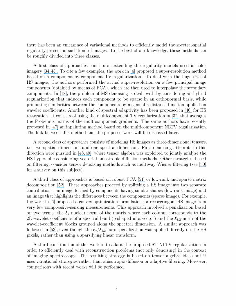
there has been an emergence of variational methods to efficiently model the spectral-spatialregularity present in such kind of images. To the best of our knowledge, these methods canbe roughly divided into three classes.

A first class of approaches consists of extending the regularity models used in colorimagery [34,45]. To cite a few examples, the work in [4] proposed a super-resolution methodbased on a component-by-component TV regularization. To deal with the huge size ofHS images, the authors performed the actual super-resolution on a few principal imagecomponents (obtained by means of PCA), which are then used to interpolate the secondarycomponents. In [18], the problem of MS denoising is dealt with by considering an hybridregularization that induces each component to be sparse in an orthonormal basis, whilepromoting similarities between the components by means of a distance function applied onwavelet coefficients. Another kind of spectral adaptivity has been proposed in [46] for HSrestoration. It consists of using the multicomponent TV regularization in [32] that averagesthe Frobenius norms of the multicomponent gradients. The same authors have recentlyproposed in [47] an inpainting method based on the multicomponent NLTV regularization.The link between this method and the proposed work will be discussed later.

A second class of approaches consists of modeling HS images as three-dimensional tensors,i.e. two spatial dimensions and one spectral dimension. First denoising attempts in thisdirection were pursued in [48,49], where tensor algebra was exploited to jointly analyze theHS hypercube considering vectorial anisotropic diffusion methods. Other strategies, basedon filtering, consider tensor denoising methods such as multiway Wiener filtering (see [50]for a survey on this subject).

A third class of approaches is based on robust PCA [51] or low-rank and sparse matrixdecomposition [52]. These approaches proceed by splitting a HS image into two separatecontributions: an image formed by components having similar shapes (low-rank image) andan image that highlights the differences between the components (sparse image). For example,the work in [6] proposed a convex optimization formulation for recovering an HS image fromvery few compressive-sensing measurements. This approach involved a penalization basedon two terms: the `∗ nuclear norm of the matrix where each column corresponds to the2D-wavelet coefficients of a spectral band (reshaped in a vector) and the `1,2-norm of thewavelet-coefficient blocks grouped along the spectral dimension. A similar approach wasfollowed in [53], even though the `∗/`1,2-norm penalization was applied directly on the HSpixels, rather than using a sparsifying linear transform.

A third contribution of this work is to adapt the proposed ST-NLTV regularization inorder to efficiently deal with reconstruction problems (not only denoising) in the contextof imaging spectroscopy. The resulting strategy is based on tensor algebra ideas but ituses variational strategies rather than anisotropic diffusion or adaptive filtering. Moreover,comparisons with recent works will be performed.

4

Outline: The paper is organized as follows. Section 2 describes the degradation modeland formulates the constrained convex optimization problem based on the non-local structuretensor. Section 3 explains how to minimize the corresponding objective function via proximaltools. Section 4 provides an experimental validation in the context of MS and HS imagerestoration. Conclusions are given in Section 5.

Notation: Let H be a real Hilbert space. Γ0(H) denotes the set of proper, lowersemicontinuous, convex functions from H to ]−∞,+∞]. Recall that a function ϕ : H →]−∞,+∞] is proper if its domain domϕ =

y ∈ H

∣∣ ϕ(y) < +∞

is nonempty. Thesubdifferential of ϕ at x ∈ H is ∂ϕ(x) =

u ∈ H

∣∣ (∀y ∈ H) 〈y − x | u〉+ ϕ(x) ≤ ϕ(y)

.The epigraph of ϕ ∈ Γ0(H) is the nonempty closed convex subset of H × R defined asepiϕ =

(y, ζ) ∈ H × R

∣∣ ϕ(y) ≤ ζ

, the lower level set of ϕ at height ζ ∈ R is the nonemptyclosed convex subset of H defined as lev≤ζ ϕ =

y ∈ H

∣∣ ϕ(y) ≤ ζ

. The projection ontoa nonempty closed convex subset C ⊂ H is, for every y ∈ H, PC(y) = argminu∈C ‖u − y‖.The indicator function ιC of C is equal to 0 on C and +∞ otherwise. Finally, Id (resp. IdN )denotes the identity operator (resp. the identity matrix of size N ×N).

2 Proposed approach

2.1 Degradation model

The R-component signal of interest is denoted by x = (x1, . . . , xR) ∈ (RN)R. In this work,each signal component will generally correspond to an image of size N = N1 × N2. Inimaging spectroscopy, R denotes the number of spectral bands. The degradation model thatwe consider in this work is

z = B(Ax) (1)

where z = (z1, . . . , zS) ∈ (RK)S denotes the degraded observations, B : (RK)S → (RK)S

models the effect of a (non-necessarily additive) noise, and A = (As,r)1≤s≤S,1≤r≤R is thedegradation linear operator with As,r ∈ RK×N , for every (s, r) ∈ 1, . . . , S × 1, . . . , R.In particular, this model can be specialized in some of the applications mentioned in theintroduction, such as super-resolution and compressive sensing, as well as unmixing asexplained in the following.

(i) Super resolution (see e.g. [4]). In this scenario, z denotes B multicomponent imagesat low-resolution and x denotes the (high-resolution) multicomponent image to berecovered. The operator A is a block-diagonal matrix with S = BR while, for everyr ∈ 1, . . . , R and b ∈ 1, . . . , B, AB(r−1)+b,r = DbTWr is a composition of a warpmatrix Wr ∈ RN×N , a camera blur operator T ∈ RN×N , and a downsampling matrixDb ∈ RK×N with K < N . The noise is assumed to be a zero-mean white Gaussian

5

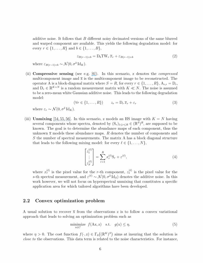
additive noise. It follows that B different noisy decimated versions of the same blurredand warped component are available. This yields the following degradation model: forevery r ∈ 1, . . . , R and b ∈ 1, . . . , B,

zB(r−1)+b = DbTWr xr + εB(r−1)+b (2)

where εB(r−1)+b ∼ N (0, σ2 IdK).

(ii) Compressive sensing (see e.g. [6]). In this scenario, z denotes the compressedmulticomponent image and x is the multicomponent image to be reconstructed. Theoperator A is a block-diagonal matrix where S = R, for every r ∈ 1, . . . , R, Ar,r = Dr,and Dr ∈ RK×N is a random measurement matrix with K N . The noise is assumedto be a zero-mean white Gaussian additive noise. This leads to the following degradationmodel:

(∀r ∈ 1, . . . , R) zr = Dr xr + εr (3)

where εr ∼ N (0, σ2 IdK).

(iii) Unmixing [54, 55, 56]. In this scenario, z models an HS image with K = N havingseveral components whose spectra, denoted by (Sr)1≤r≤R ∈ (RS)R, are supposed to beknown. The goal is to determine the abundance maps of each component, thus theunknown x models these abundance maps. R denotes the number of components andS the number of spectral measurements. The matrix A has a block diagonal structurethat leads to the following mixing model: for every ` ∈ 1, . . . , N,z

(`)1...

z(`)S

=R∑r=1

x(`)r Sr + ε(`), (4)

where x(`)r is the pixel value for the r-th component, z

(`)s is the pixel value for the

s-th spectral measurement, and ε(`) ∼ N (0, σ2 IdS) denotes the additive noise. In thiswork however, we will not focus on hyperspectral unmixing that constitutes a specificapplication area for which tailored algorithms have been developed.

2.2 Convex optimization problem

A usual solution to recover x from the observations z is to follow a convex variationalapproach that leads to solving an optimization problem such as

minimizex∈C

f(Ax, z) s.t. g(x) ≤ η, (5)

where η > 0. The cost function f(·, z) ∈ Γ0

((RK)S

)aims at insuring that the solution is

close to the observations. This data term is related to the noise characteristics. For instance,

6

standard choices for f are a quadratic function for an additive Gaussian noise, an `1-normwhen a Laplacian noise is involved, and a Kullback-Leibler divergence when dealing withPoisson noise. The function g ∈ Γ0

((RN)R

)allows us to impose some regularity on the

solution. Some possible choices for this function have been mentioned in the introduction.

Note that state-of-the-art methods often deal with the regularized version of Problem (5),that is

minimizex∈C

f(Ax, z) + λg(x), (6)

where λ > 0. Actually, both formulations are equivalent for some specific values of λ and η.As mentioned in the introduction, the advantage of the constrained formulation is that thechoice of η may be easier, since it is directly related to the properties of the signal to berecovered.

Finally, C denotes a nonempty closed convex subset of (RN)R, which can be used forpurposes like constraining the dynamics range of the signal to be recovered.

2.3 Structure Tensor regularization

In this work, we propose to model the spatial and spectral dependencies in multicomponentimages by introducing a regularization grounded on the use of a matrix norm, which isdefined as (

∀x ∈ (RN)R)

g(x) =N∑`=1

τ`‖F`B`x‖p, (7)

where ‖ · ‖p denotes the Schatten p-norm with p ≥ 1, (τ`)1≤`≤N are positive weights, and, forevery ` ∈ 1, . . . , N,

(i) block selection: the operator B` : (RN)R → RQ2×R selects Q × Q blocks of eachcomponent (including the pixel `) and rearranges them in a matrix of size Q2 ×R, soleading to

Y(`) =

x(n`,1)1 . . . x

(n`,1)R

......

x(n`,Q2 )

1 . . . x(n`,Q2 )

R

(8)

where W` = n`,1, . . . , n`,Q2 is the set of positions located into the window around `,and Q > 1;1

(ii) block transform: the operator F` : RQ2×R → RM`×R denotes an analysis transformthat achieves a sparse representation of grouped blocks, yielding

X(`) = F`Y(`), (9)

1The image borders are handled by symmetric extension.

7

where M` ≤ Q2.

The resulting structure tensor regularization reads

g(x) =N∑`=1

τ` ‖X(`)‖p. (10)

Let us denote by

σX(`) =(σ(m)

X(`)

)1≤m≤M`

, with M` = minM`, R, (11)

the singular values of X(`) ordered in decreasing order. When p ∈ [1,+∞[, we have

g(x) =N∑`=1

τ`

M∑m=1

(σ(m)

X(`)

)p1/p

, (12)

whereas, when p = +∞,

g(x) =N∑`=1

τ` σ(1)

X(`) . (13)

When p = 1, the Schatten norm reduces to the nuclear norm. In such a case, the structuretensor regularization induces a low-rank approximation of matrices (X(`))1≤`≤N (see [57] fora survey on singular value decomposition).

The structure tensor regularization proposed in (9) generalizes several state-of-the-artregularization strategies, as explained below.

2.3.1 ST-TV

We retrieve the multicomponent TV regularization [32,34,46] by setting F` to the operator

which, for each component index r ∈ 1, . . . , R, computes the difference between x(`)r and

its horizontal/vertical nearest neighbours (x(`1)r , x

(`2)r ), yielding the matrix

X(`)TV

=

[x(`)1 − x

(`1)1 . . . x

(`)R − x

(`1)R

x(`)1 − x

(`2)1 . . . x

(`)R − x

(`2)R

](14)

with M` = 2. This implies a 2 × 2 block selection operator (i.e., Q = 2). Note that theregularization proposed in [46] is a special case of this ST-TV constraint arising when p = 2.We will refer to it as Hyperspectral-TV in Section 4. Finally, note that the regularizationused in [4] is intrinsically different from the ST-TV described above, as the former amountsto summing up the smoothed TV [58] evaluated separately over each component.

8

2.3.2 ST-NLTV

We extend the NLTV regularization [12] to multicomponent images by setting F` to theoperator which, for each component index r ∈ 1, . . . , R, computes the weighted difference

between x(`)r and some other pixel values. This results in the matrix

X(`)NLTV

=[ω`,n(x(`)r − x(n)r )

]n∈N`,1≤r≤R

, (15)

where N` ⊂ W` \ ` denotes the non-local support of the neighbourhood of `. Here, M`

corresponds to the size of this support. Note that the regularization in [47] appears as aspecial case of the proposed ST-NLTV arising when p = 2 and the local window is fully used(M` = Q2). We will refer to it as Multichannel-NLTV in Section 4.

For every ` ∈ 1, . . . , N and n ∈ N`, the weight ω`,n > 0 depends on the similaritybetween patches built around the pixels ` and n of the image to be recovered. Since thedegradation process in (1) may involve some missing data, we follow a two-step approach inorder to estimate these weights. In the first step, the ST-TV regularization is used in orderto obtain an estimate x of the target image. This estimate subsequently serves in the secondstep to compute the weights through a self-similarity measure as follows:

ω`,n = ω` exp(−δ−2 ‖L`x− Lnx‖22

), (16)

where δ > 0, L` (resp. Ln) selects a Q× Q×R patch centered at position ` (resp. n) aftera linear processing of the image depending on the position ` (resp. n), and the constantω` > 0 is set so as to normalize the weights (i.e.

∑n∈N`

ω`,n = 1). In particular, the operatorL` (resp. Ln) may involve a convolution with either a Gaussian function with mean ` (resp.n) and a given variance [11], or a set of low-pass Gaussian filters whose variances increase asthe spatial distance from the patch center ` (resp. n) grows [59]. For every ` ∈ 1, . . . , N,the neighbourhood N` is built according to the procedure described in [60]. In practice, we

limit the size of the neighbourhood, so that M (`) ≤M (the values chosen for Q, Q, δ and Mare indicated in Section 4).

3 Optimization method

Within the proposed constrained optimization framework, Problem (5) can be reformulatedas follows:

minimizex∈C

f(Ax, z) s. t. Φ x ∈ D, (17)

where Φ is the linear operator defined as

Φ: x 7→ X =

F1B1x

...

FNBNx

X(1)

X(N)

(18)

9

with X ∈ RM×R and M = M1 + · · ·+MN , while D is the closed convex set defined as

D =

X ∈ RM×R ∣∣ N∑`=1

τ`‖X(`)‖p ≤ η. (19)

In recent works, iterative procedures were proposed to deal with an `1- or `1,2-ball constraint[42] and an `1,∞-ball constraint [43]. Similar techniques can be used to compute the projectiononto D, but a more efficient approach consists of adapting the epigraphical splitting techniqueinvestigated in [61,62,63,64].

3.1 Epigraphical splitting

Epigraphical splitting applies to a convex set that can be expressed as the lower level set ofa separable convex function, such as the constraint set D defined in (19). Some auxiliaryvariables are introduced into the minimization problem, so that the constraint D can beequivalently re-expressed as the intersection of two convex sets. More specifically, differentsplitting solutions need to be proposed according to the involved Schatten p-norm:

(i) in the case when p = 1, since

X ∈ D ⇔N∑`=1

M∑m=1

τ`

∣∣∣σ(m)

X(`)

∣∣∣ ≤ η, (20)

we propose to introduce an auxiliary vector ζ ∈ RM , with ζ = (ζ(`,m))1≤`≤N,1≤m≤M`

and

M = M1 + . . .+ MN , in order to rewrite (20) as(∀` ∈ 1, . . . , N)(∀m ∈ 1, . . . , M`)

∣∣∣σ(m)

X(`)

∣∣∣ ≤ ζ(`,m),

N∑`=1

M∑m=1

τ` ζ(`,m) ≤ η.

(21)

Consequently, Constraint (20) is decomposed in two convex sets: a union of epigraphs

E =

(X, ζ) ∈ RM×R × RM∣∣ (∀` ∈ 1, . . . , N)(∀m ∈ 1, . . . , M`) (σ

(m)

X(`) , ζ(`,m)) ∈ epi |·|

,

(22)and the closed half-space

W =ζ ∈ RM

∣∣ N∑`=1

M∑m=1

τ` ζ(`,m) ≤ η

. (23)

10

(ii) in the case when p > 1, since

X ∈ D ⇔N∑`=1

τ` ‖σX(`)‖p ≤ η, (24)

we define an auxiliary vector ζ = (ζ(`))1≤`≤N ∈ RN of smaller dimension N , and werewrite Constraint (24) as

(∀` ∈ 1, . . . , N) ‖σX(`)‖p ≤ ζ(`),N∑`=1

τ` ζ(`) ≤ η.

(25)

Similarly to the previous case, Constraint (24) is decomposed in two convex sets: aunion of epigraphs

E =

(X, ζ) ∈ RM×R × RN∣∣ (∀` ∈ 1, . . . , N)(σX(`) , ζ(`)) ∈ epi ‖ · ‖p

, (26)

and the closed half-space

W =ζ ∈ RN

∣∣ N∑`=1

τ` ζ(`) ≤ η

. (27)

3.2 Epigraphical projection

The epigraphical splitting technique allows us to reformulate Problem (17) in a more tractableway, as follows

minimize(x,ζ)∈C×W

f(Ax, z) s. t. (Φ x, ζ) ∈ E. (28)

The advantage of such a decomposition is that the projections PE and PW onto E and W mayhave closed-form expressions. Indeed, the projection PW is well-known [65], while propertiesof the projection PE are summarized in the following proposition, which is straightforwardlyproved.

Proposition 3.1. For every ` ∈ 1, . . . , N, let

X(`) = U(`)S(`)(V(`)

)>(29)

be the Singular Value Decomposition of X(`) ∈ RM`×R, where

• (U(`))>U(`) = IdM`,

•(V(`)

)>V(`) = IdM`

,

11

• S(`) = Diag(s(`)), with s(`) = (σ(m)

X(`))1≤m≤M`.

Then,

PE(X, ζ) =(

U(`)T(`)(V(`)

)>, θ(`)

)1≤`≤N

, (30)

where T(`) = Diag(t(`)) and,

(i) in the case p = 1, for every m ∈ 1, . . . , M`

(t(`,m), θ(`,m)) = Pepi |·|(s(`,m), ζ(`,m)), (31)

(ii) in the case p > 1,(t(`), θ(`)) = Pepi ‖·‖p(s(`), ζ(`)). (32)

The above result states that the projection onto the epigraph of the `1,p matrix norm can bededuced from the projection onto the epigraph of the `1,p vector norm. It turns out thatclosed-form expressions of the latter projection exist when p ∈ 1, 2,+∞ [61]. For example,

for every (s(`), ζ(`)) ∈ RM` × R,

Pepi ‖·‖2(s(`), ζ(`)) =

(0, 0), if ‖s(`)‖2 < −ζ(`),(s(`), ζ(`)), if ‖s(`)‖2 < ζ(`),

β(`)(s(`), ‖s(`)‖2

), otherwise,

(33)

where β(`) =1

2

(1 +

ζ(`)

‖s(`)‖2

). Note that the closed-form expression for p = 1 can be derived

from (33). Moreover,Pepi ‖·‖∞(s(`), ζ(`)) = (t(`), θ(`)), (34)

where, for every t(`) = (t(`,m))1≤m≤M`∈ RM` ,

t(`,m) = minσ(m)

X(`) , θ(`), (35)

θ(`) =max

(ζ(`) +

∑M`

k=k`ν(`,k), 0

)M` − k` + 2

. (36)

Hereabove, (ν(`,k))1≤k≤M`is a sequence of real numbers obtained by sorting (σ

(m)

X(`))1≤m≤M`in

ascending order (by setting ν(`,0) = −∞ and ν(`,M`+1) = +∞), and k` is the unique integerin 1, . . . , M` + 1 such that

ν(`,k`−1) <ζ(`) +

∑M`

k=k`ν(`,k)

M` − k` + 2≤ ν(`,k`) (37)

12

(with the convention∑M(`)

k=M(`)+1· = 0).

Note that the computation of the SVD can be avoided when p = 2, as the Frobeniusnorm is equal to the `2-norm of the vector of all matrix elements.

3.3 Proposed algorithm

The solution of (28) requires an efficient algorithm for dealing with large scale problemsinvolving nonsmooth functions and linear operators that are non-necessarily circulant. Forthis reason, we resort here to proximal algorithms [66,67, 68,69, 70,71,72, 73,74, 75,76, 77,78,79, 80, 81, 82]. The key tool in these methods is the proximity operator [83] of a functionφ ∈ Γ0(H) on a real Hilbert space, defined as

(∀u ∈ H) proxφ(u) = argminv∈H

1

2‖v− u‖2 + φ(v). (38)

The proximity operator can be interpreted as an implicit subgradient step for the functionφ, since p = proxφ(u) is uniquely defined through the inclusion u− p ∈ ∂φ(p). Proximityoperators enjoy many interesting properties [67]. In particular, they generalize the notionof projection onto a closed convex set C, in the sense that proxιC = PC . Hence, proximalmethods provide a unifying framework that allows one to address a wide class of convexoptimization problems involving non-smooth penalizations and hard constraints.

Among the wide array of existing proximal algorithms, we employ the primal-dualM+LFBF algorithm recently proposed in [79], which is able to address general convexoptimization problems involving nonsmooth functions and linear operators without requiringany matrix inversion. This algorithm is able to solve numerically:

minimizev∈H

φ(v) +I∑i=1

ψi(Tiv) + ϕ(v). (39)

where φ ∈ Γ0(H), for every i ∈ 1, . . . , I, Ti : H → Gi is a bounded linear operator,ψi ∈ Γ0(Gi) and ϕ : H → ]−∞,+∞] is a convex differentiable function with a µ-Lipschitziangradient. Our minimization problem fits nicely into this framework by settingH = (RN )R×RL

with

L =

M if p = 1,

N if p > 1,(40)

and v = (x, ζ). Indeed, we set I = 2, G1 = RM×R × RL and G2 = (RK)S in (39), the linearoperators reduce to

T1 =

[Φ 00 IdL

], T2 =

[A 0

], (41)

13

and the functions are as follows

(∀(x, ζ) ∈ (RN)R × RL) φ(x, ζ) = ιC(x) + ιW (ζ),

(∀(x, ζ) ∈ (RN)R × RL) φ(x, ζ) = ιC(x) + ιW (ζ),

(∀(X, ζ) ∈ RM×R × RL) ψ1(X, ζ) = ιE(X, ζ),

(∀y ∈ (RK)S) ψ2(y) = f(y, z),

(∀(x, ζ) ∈ (RN)R × RL) ϕ(x, ζ) = 0.

(42)

The iterations associated with Problem (28) are summarized in Algorithm 1, where A> andΦ> designate the adjoint operators of A and Φ. The sequence (x[t])t∈N generated by thealgorithm is guaranteed to converge to a solution to (28) (see [79]).

Algorithm 1 M+LFBF for solving Problem (28)

InitializationY

[0]1 ∈ RM×R, ν[0]1 ∈ RL

y[0]2 ∈ (RK)S

x[0] ∈ (RN )R, ζ [0] ∈ RL

θ =√‖A‖2 + max‖Φ‖2, 1

ε ∈]0, 1θ+1 [

For t = 0, 1, . . .

γt ∈[ε,

1− εθ

](

x[t], ζ [t])

=(

x[t], ζ [t])− γt

(Φ>Y

[t]1 + A>y

[t]2 , ν

[t])(

p[t], ρ[t])

=(PC(x[t]), PW (ζ [t])

)(

Y[t]

1 , ν[t]1

)=(

Y[t]1 , ν

[t]1

)+ γt

(Φx[t], ζ [t]

)(

Y[t]

1 , ν[t]1

)=(

Y[t]

1 , ν[t]1

)− γtPE

(Y

[t]

1 /γt, ν[t]1 /γt

)(

Y[t+1]1 , ν

[t+1]1

)=(

Y[t]

1 , ν[t]1

)+ γt

(Φ(p[t] − x[t]), ρ[t] − ζ [t]

)y[t]2 = y

[t]2 + γtAx[t]

y[t]2 = y

[t]2 − γt proxγ−1

t f

(y[t]2 /γt

)y[t+1]2 = y

[t]2 + γtA(p[t] − x[t])(

x[t], ζ [t])

=(

p[t], ρ[t])− γt

(Φ>Y

[t]

1 + A>y[t]2 , ν

[t]1

)(x[t+1], ζ [t+1]

)=(

x[t] − x[t] + x[t], ζ [t] − ζ [t] + ζ [t])

3.4 Approach based on ADMM

Note that an alternative approach to deal with Problem (17) consists of employing theAlternating Direction Method of Multipliers (ADMM) [84] or one of its parallel versions

14

[73,74,85,86,87,88], sometimes referred to as the Simultaneous Direction Method of Multipliers(SDMM). Although these algorithms are appealing, they require to invert the operatorId +Φ>Φ + A>A, which makes them less attractive than primal-dual algorithms for solvingProblem (17). Indeed, this matrix is not diagonalizable in the DFT domain (due to the formof Φ), which rules out efficient inversion techniques such as those employed in [86,89,90]. Tothe best of our knowledge, this issue can be circumvented in specific cases only, for examplewhen Φ denotes the NLTV operator defined in (15). In this case, one may resort to thesolution in [18,91], which consists of decomposing Φ as follows:

Φ = Ω

G1...

GQ2−1

︸ ︷︷ ︸

G

, (43)

where, for every q ∈ 1, . . . , Q2 − 1, Gq : (RN)R → RN×R is a discrete difference operatorand Ω ∈ RM×N(Q2−1) is a weighted block-selection operator. Consequently, Problem (17)can be equivalently reformulated by introducing an auxiliary variable ξ = Φx ∈ RM×R in theminimization problem, yielding

minimize(x,ξ)∈C×D

f(Ax, z) s. t. (Gx, ξ) ∈ V, (44)

where V =

(X, ξ) ∈ RN(Q2−1)×R × RM×R∣∣ ΩX = ξ

. The iterations associated to SDMM

are illustrated in Algorithm 2.

It is worth emphasizing that SDMM still requires to compute the projection onto D,which may be done by either resorting to specific numerical solutions [42, 43, 92, 93] oremploying the epigraphical splitting technique presented in Section 3.1. However, accordingto our simulations (see Section 4.1), both approaches are slower than Algorithm 1.

4 Numerical results

In this section, we numerically evaluate the ST-NLTV regularization proposed in Section 2and compare Algorithm 1 with implementations of two state-of-the-art methods:

• Hyperspectral TV (H-TV) [46] – see Section 2.3.1,

• Multichannel NLTV (M-NLTV) [47] – see Section 2.3.2.

To this end, two scenarios are addressed: a compressive sensing scenario by using thedegradation model (3) where the measurement operator reduces to a random decimation,

15

Algorithm 2 SDMM for solving Problem (44)

Initializationy[0]1 ∈ (RN )R,Y

[0]2 ∈ RM×R, y[0]

3 ∈ (RK)S

y[0]1 ∈ (RN )R,Y

[0]2 ∈ RM×R, y[0]

3 ∈ (RK)S

χ[0]1 ∈ RM×R, χ[0]

2 ∈ RM×R

χ[0]1 ∈ RM×R, χ[0]

2 ∈ RM×RH = Id +G>G + A>A

For t = 0, 1, . . .

γt ∈ ]0,+∞[

x[t] = H−1[y[t]1 − y

[t]1 + G>(Y

[t]2 −Y

[t]2 ) + A>(y

[t]3 − y

[t]3 )]

ξ[t] = 12

(χ[t]1 − χ

[t]1

)+ 1

2

(χ[t]2 − χ

[t]2

)y[t+1]1 = PC

(x[t] + y

[t]1

)χ[t+1]1 = PD

(ξ[t] + χ

[t]1

)(Y

[t+1]2 , χ

[t+1]2

)= PV (Gx[t] + Y

[t]2 , ξ

[t] + χ[t]2 )

y[t+1]3 = proxγtf

(Ax[t] + y

[t]3

)y[t+1]1 = y

[t]1 + x[t] − y

[t+1]1

χ[t+1]1 = χ

[t]1 + ξ[t] − χ[t+1]

1

Y[t+1]2 = Y

[t]2 + Gx[t] −Y

[t+1]2

χ[t+1]2 = χ

[t]2 + ξ[t] − χ[t+1]

2

y[t+1]3 = y

[t]3 + Ax[t] − y

[t+1]3

and a restoration scenario by replacing the measurement operator in (3) with a decimatedconvolution. For reproducibility purposes, we use several publicly available multispectraland hyperspectral images.2 The SNR index is used to give a quantitative assessment of theresults of the simulated experiments. In particular, we report the SNR computed over all theimage components and the mean SNR (M-SNR) computed by averaging the SNR evaluatedcomponent-by-component.

In our experiments, the images are degraded by (spectrally independent) additive zero-mean white Gaussian noises. Before degrading the original images, the pixels of eachcomponent are normalized between [0, 255]. Therefore, the fidelity term related to the noiseneg-log-likelihood is f = ‖A · −z‖22 and the dynamics range constraint set C imposes that

the pixel values belong to [0, 255]. For the ST constraints, we set Q = 11, Q = 5, δ = 35 andM = 14, as this setting was observed to yield the best numerical results.

Extensive tests have been carried out on several images of different sizes. The SNR andM-SNR indices obtained by using the proposed `1-ST-TV and `1-ST-NLTV regularization

2https://engineering.purdue.edu/∼biehl/MultiSpec/hyperspectral.html

16

constraints are collected in Tables 1 and 2 for the two degradation scenarios mentioned above.In addition, a comparison is performed between our method and the H-TV and M-NLTValgorithms mentioned above (using an M+LFBF implementation). The hyper-parameterfor each method (the bound η for the ST constraint in our algorithm) was hand-tuned inorder to achieve the best SNR values. The best results are highlighted in bold. Moreover,a component-by-component comparison of two hyperspectral images is made in Figure 2,while a visual comparison of a component from the image hydice is displayed in Figure 1.

The aforementioned results demonstrate the interest of combining the non-locality princi-ple with structure-tensor smoothness measures. Indeed, `1-ST-NLTV proves to be the mosteffective regularization with gains in SNR (up to 1.4 dB) with respect to M-NLTV, whichin turn is comparable with `1-ST-TV. The better performance of `1-ST-NLTV seems to berelated to its ability to better preserve edges and thin structures present in images, whilepreventing component smearing.

(a) Component r = 81. (b) H-TV: 11.78 dB. (c) `1-ST-TV: 12.98 dB.

(d) Noisy. (e) M-NLTV: 12.76 dB. (f) `1-ST-NLTV: 14.36 dB.

Figure 1: Visual comparison of the hyperspectral image hydice reconstructed with H-TV [46],`1-ST-TV, M-NLTV [47] and `1-ST-NLTV. Degradation: compressive sensing scenarioinvolving an additive zero-mean white Gaussian noise with std. deviation 5 and 90% ofdecimation (N = 65536, R = 191, K = 6553 and S = 191).

17

Table 1: SNR (dB) – Mean SNR (dB) of reconstructed images (Degradation: std. deviation= 5, decimation = 90%).

image size H-TV [46] `1-ST-TV M-NLTV [47] `1-ST-NLTV

Hydice 256× 256× 191 10.65 – 09.87 11.93 – 11.16 11.57 – 10.76 12.98 – 12.11Indian Pine 145× 145× 200 17.31 – 17.00 18.46 – 18.24 17.62 – 17.34 19.53 – 19.49Little Coriver 512× 512× 7 17.81 – 18.20 18.49 – 18.83 18.46 – 18.90 19.88 – 20.18Mississippi 512× 512× 7 18.27 – 18.07 18.60 – 18.37 18.94 – 18.59 19.56 – 19.28Montana 512× 512× 7 22.49 – 20.97 22.68 – 21.15 22.85 – 21.29 23.31 – 21.76Rio 512× 512× 7 16.48 – 15.29 16.65 – 15.48 16.82 – 15.64 17.20 – 16.05Paris 512× 512× 7 14.85 – 14.31 14.94 – 14.39 15.05 – 14.53 15.36 – 14.82

Table 2: SNR (dB) – mean SNR (dB) of restored images (Degradation: std. deviation = 5,blur = 5× 5, decimation = 70%).

image size H-TV [46] `1-ST-TV M-NLTV [47] `1-ST-NLTV

Hydice 256× 256× 191 13.76 – 12.90 14.30 – 13.50 13.84 – 12.98 14.84 – 14.08Indian Pine 145× 145× 200 19.80 – 19.65 20.22 – 20.13 19.73 – 19.57 20.43 – 20.41Little Coriver 512× 512× 7 21.35 – 21.88 21.62 – 22.01 21.31 – 22.00 21.99 – 22.49Mississippi 512× 512× 7 21.12 – 20.29 21.21 – 20.27 21.41 – 20.52 21.65 – 20.83Montana 512× 512× 7 24.80 – 23.37 24.82 – 23.31 24.96 – 23.53 25.18 – 23.72Rio 512× 512× 7 18.62 – 17.50 18.57 – 17.48 18.57 – 17.60 18.87 – 17.80Paris 512× 512× 7 16.68 – 16.55 16.80 – 16.53 16.73 – 16.60 17.05 – 16.81

0 50 100 1508

10

12

14

16

L1−ST−TV

L1−ST−NLTV

M−NLTV

HTV

(a) SNR (dB) vs component index (image: hy-dice).

0 50 100 150 20012

14

16

18

20

22

24

L1−ST−TV

L1−ST−NLTV

M−NLTV

HTV

(b) SNR (dB) vs component index (image: indianpine).

Figure 2: Quantitative comparison of two hyperspectral images reconstructed with H-TV [46], `1-ST-TV, M-NLTV [47] and `1-ST-NLTV. Degradation: compressive sensingscenario involving an additive zero-mean white Gaussian noise with std. deviation 5 and 90%of decimation.

18

4.1 Comparison with SDMM

To complete our analysis, we compare the execution time of Algorithm 1 with respect tothree alternative solutions:

• M+LFBF applied to Problem (17) by computing the projection onto D via the iterativeprocedure in [42];

• SDMM applied to Problem (44) by computing the projection onto D via the iterativeprocedure in [42] (Algorithm 2);

• SDMM applied to Problem (44) after that D is replaced by the constraints E and W .

We would like to emphasize that all the aforementioned algorithms solve exactly Problem (17),hence they produce equivalent results (i.e. they converge to the same solution). Our objectivehere is to empirically demonstrate that the epigraphical splitting technique and primal-dualproximal algorithms constitute a competitive choice for the problem at hand.

We present the results obtained with the image indian pine, since a similar behaviourwas observed for other images. The stopping criterion is set to ‖x[i+1] − x[i]‖ ≤ 10−5‖x[i]‖.Our codes were developed in MATLAB R2011b (the operators Φ and Φ> being implementedin C using mex files) and executed on an Intel Xeon CPU at 2.80 GHz and 8 GB of RAM.For the `1-ball projectors needed by the direct method to compute the projection onto D,we used the software publicly available on-line (at www.cs.ubc.ca/∼mpf/spgl1) [42].

Fig. 3 shows the relative error ‖x[i] − x[∞]‖/‖x[∞]‖ as a function of the computationaltime, where x[∞] denotes the solution computed with a stopping criterion of 10−5. Theseplots indicate that the epigraphical approach yields a faster convergence than the direct onefor both SDMM and M+LFBF, the latter being much faster than the former. This can beexplained by the computational cost of the subiterations required by the direct projectiononto the `1-ball. Note that these conclusions extend to all images in the dataset.

The results in Fig. 3 refer to the constraint bound η that achieves the best SNR indices.In practice, the optimal bound may not be known precisely. Although it is out of the scopeof this paper to devise an optimal strategy to set this bound, it is important to evaluatethe impact of its choice on our method performance. In Tables 3 and 4, we compare theepigraphical approach with the direct computation of the projections (via standard iterativesolutions) for different choices of η. For better readability, the values of η are expressed as amultiplicative factor of the ST-TV and ST-NLTV semi-norms of the original image. Theexecution times indicate that the epigraphical approach yields a faster convergence thanthe direct approach for SDMM and M+LFBF. Moreover, the numerical results show thaterrors within ±10% from the optimal value for η lead to SNR variations within 2.6%. Werefer to [61] for an extensive comparison between the epigraphical approach and the directcomputation of the projections.

19

0 200 400 600 800 100010

−5

10−4

10−3

10−2

10−1

100

SDMMSDMM (epi)M+LFBFM+LFBF (epi)

(a) `1-ST-TV.0 500 1000 1500 2000 2500 3000 3500 4000

10−5

10−4

10−3

10−2

10−1

100

SDMMSDMM (epi)M+LFBFM+LFBF (epi)

(b) `1-ST-NLTV.

Figure 3: Comparison between epigraphical and direct methods: ‖x[i]−x[∞]‖‖x[∞]‖ vs time (Degra-

dation: std. deviation = 5, decimation = 90%).

Table 3: Results for the `1-ST-TV constraint and some values of η (Degradation: std.deviation = 5, decimation = 90%)

η SNR (dB) – M-SNR (dB)

SDMM M+LFBF

direct epigraphicalspeed up

direct epigraphicalspeed up

# iter. sec. # iter. sec. # iter. sec. # iter. sec.

0.3 18.28 – 18.05 394 499.97 377 378.38 1.32 327 333.18 281 252.38 1.320.4 18.46 – 18.24 838 1066.24 698 701.03 1.52 733 735.36 621 558.37 1.320.5 16.48 – 16.10 647 830.14 173 173.72 4.78 523 528.39 138 124.07 4.25

Table 4: Results for the `1-ST-NLTV constraint and some values of η (Degradation: std.deviation = 5, decimation = 90%)

η SNR (dB) – M-SNR (dB)

SDMM M+LFBF

direct epigraphicalspeed up

direct epigraphicalspeed up

# iter. sec. # iter. sec. # iter. sec. # iter. sec.

Neighbourhood size: Q = 30.2 18.94 – 18.82 1000 4390.05 1000 3421.04 1.28 170 452.78 180 411.28 1.100.3 19.39 – 19.32 1000 4414.94 1000 3417.18 1.29 243 649.31 236 534.50 1.210.4 19.30 – 19.22 941 4186.20 1000 3441.78 1.22 445 1190.30 442 957.63 1.24

Neighbourhood size: Q = 50.2 19.21 – 19.14 1000 15595.51 1000 11298.05 1.38 171 777.38 171 711.63 1.090.3 19.53 – 19.49 1000 15338.36 1000 11174.68 1.37 275 1257.71 268 1143.35 1.100.4 19.33 – 19.25 1000 15403.72 1000 11442.47 1.35 500 2285.51 479 2043.51 1.12

20

5 Conclusions

We have proposed a new regularization for multicomponent images that is a combinationof non-local total variation and structure tensor. The resulting image recovery problemhas been formulated as a constrained convex optimization problem and solved through anovel epigraphical projection method using primal-dual proximal algorithms. The obtainedresults demonstrate the better performance of structure tensor and non-local gradients overa number of multispectral and hyperspectral images. Our results also show that the nuclearnorm has to be preferred over the Frobenius norm for hyperspectral image recovery problems.Furthermore, the experimental part indicates that the epigraphical method converges fasterthan the approach based on the direct computation of the projections via standard iterativesolutions. In both cases, the proposed algorithm turns out to be faster than solutions basedon the Alternating Direction Method of Multipliers, suggesting that primal-dual proximalalgorithms constitute a good choice in practice to deal with multicomponent image recoveryproblems.

References

[1] P. Valero, S. Salembier and J. Chanussot, “Hyperspectral image representation andprocessing with binary partition trees,” IEEE Trans. Image Process., vol. 22, no. 4, pp.1430–1443, Apr. 2013.

[2] R. Molina, J. Nunez, F. J. Cortijo, and J. Mateos, “Image restoration in astronomy: ABayesian perspective,” IEEE Signal Proc. Mag., vol. 18, no. 2, pp. 11–29, Mar. 2001.

[3] C. Vonesch, F. Aguet, J.-L. Vonesch, and M. Unser, “The colored revolution ofbioimaging,” IEEE Signal Proc. Mag., vol. 23, no. 3, pp. 20–31, May 2006.

[4] H. Zhang, L. Zhang, and H. Shen, “A super-resolution reconstruction algorithm forhyperspectral images,” Elsevier Sig. Proc., vol. 92, no. 9, pp. 2082–2096, Sept. 2012.

[5] H. Rauhut, K. Schnass, and P. Vandergheynst, “Compressed sensing and redundantdictionaries,” IEEE Trans. Inform. Theory, vol. 54, no. 5, pp. 2210–2219, May 2008.

[6] M. Golbabaee and P. Vandergheynst, “Hyperspectral image compressed sensing vialow-rank and joint-sparse matrix recovery,” in Proc. Int. Conf. Acoust., Speech SignalProcess., Kyoto, Japan, Mar. 2012.

[7] J. Oliveira, M.A.T. Figueiredo, and J. Bioucas-Dias, “Parametric blur estimation forblind restoration of natural images: linear motion and out-of-focus,” IEEE Trans. ImageProcess., vol. 23, pp. 466–477, 2014.

21

[8] L. Rudin, S. Osher, and E. Fatemi, “Nonlinear total variation based noise removalalgorithms,” Physica D, vol. 60, no. 1-4, pp. 259–268, Nov. 1992.

[9] P. L. Combettes and J.-C. Pesquet, “Image restoration subject to a total variationconstraint,” IEEE Trans. Image Process., vol. 13, no. 9, pp. 1213–1222, Sept. 2004.

[10] K. Bredies, K. Kunisch, and T. Pock, “Total generalized variation,” SIAM J. onImaging Sci., vol. 3, no. 3, pp. 492–526, Sept. 2010.

[11] A. Buades, B. Coll, and J. Morel, “A review of image denoising algorithms, with a newone,” Multiscale Model. and Simul., vol. 4, no. 2, pp. 490–530, 2005.

[12] G. Gilboa and S. Osher, “Nonlocal operators with applications to image processing,”Multiscale Model. and Simul., vol. 7, no. 3, pp. 1005, 2009.

[13] V. Duval, J.-F. Aujol, and Y. Gousseau, “A bias-variance approach for the non-localmeans,” SIAM J. on Imaging Sci., vol. 4, no. 2, pp. 760–788, 2011.

[14] S. Mallat, A wavelet tour of signal processing, Academic Press, San Diego, USA, 1997.

[15] A. Benazza-Benyahia and J.-C. Pesquet, “Building robust wavelet estimators formulticomponent images using Stein’s principle,” IEEE Trans. Image Process., vol. 14,no. 11, pp. 1814 – 1830, 2005.

[16] C. Chaux, L. Duval, A. Benazza-Benyahia, and J.-C. Pesquet, “A nonlinear Stein-basedestimator for multichannel image denoising,” IEEE Trans. Signal Process., vol. 56, no.8, pp. 3855 – 3870, 2008.

[17] C. Chaux, A. Benazza-Benyahia, J.-C. Pesquet, and Duval, “Wavelet transform for thedenoising of multivariate images,” pp. 203–237. ISTE Ltd and John Wiley & Sons Inc,2010.

[18] L. M. Briceno-Arias, P. L. Combettes, J.-C. Pesquet, and N. Pustelnik, “Proximalalgorithms for multicomponent image recovery problems,” J. Math. Imag. Vis., vol. 41,no. 1, pp. 3–22, Sept. 2011.

[19] A. Foi, V. Katkovnik, and K. Egiazarian, “Pointwise shape-adaptive DCT for high-quality denoising and deblocking of grayscale and color images,” IEEE Trans. ImageProcess., vol. 16, no. 5, pp. 1395 – 1411, May 2007.

[20] K. Dabov, A. Foi, V. Katkovnik, and K. Egiazarian, “Image denoising by sparse 3Dtransform-domain collaborative filtering,” IEEE Trans. Image Process., vol. 16, no. 8,pp. 2080 – 2095, Aug. 2007.

[21] M. Maggioni, V. Katkovnik, K. Egiazarian, and A. Foi, “A nonlocal transform-domainfilter for volumetric data denoising and reconstruction,” IEEE Trans. Image Process.,vol. 22, no. 1, pp. 119 – 133, Jan. 2013.

22

[22] A. Danielyan, V. Katkovnik, and K. Egiazarian, “BM3D frames and variational imagedeblurring,” IEEE Trans. Image Process., vol. 21, no. 4, pp. 1715–1728, 2012.

[23] P. Blomgren and T.F. Chan, “Color TV: total variation methods for restoration ofvector-valued images,” IEEE Trans. Image Process., vol. 7, no. 3, pp. 304–309, Mar.1998.

[24] H. Attouch, G. Buttazzo, and G. Michaille, Variational Analysis in Sobolev and BVSpaces: Applications to PDEs and Optimization, MPS-SIAM Series on Optimization,2006.

[25] C. Zach, T. Pock, and H. Bischof, “A duality based approach for realtime TV-L1 opticalflow,” in Proceedings of DAGM Symposium on Pattern Recognition, Berlin, Heidelberg,Sep. 12-14, 2007, pp. 214–223, Springer-Verlag.

[26] V. Duval, J.-F. Aujol, and L. Vese, “Projected gradient based color image decomposition,”in Scale Space and Variational Methods in Computer Vision, vol. 5567 of Lecture Notesin Computer Science, pp. 295–306. Springer Berlin / Heidelberg, 2009.

[27] S. Di Zenzo, “A note on the gradient of a multi-image,” Computer Vision, Graphicsand Image Processing, vol. 33, no. 1, pp. 116–125, Jan. 1986.

[28] G. Sapiro and D. L. Ringach, “Anisotropic diffusion of multivalued images withapplications to color filtering,” IEEE Trans. Image Process., vol. 5, no. 11, pp. 1582–1586, Nov. 1996.

[29] N. Sochen, R. Kimmel, and R. Malladi, “A general framework for low level vision,”IEEE Trans. Image Process., vol. 7, no. 3, pp. 310–318, Mar. 1998.

[30] J. Weickert, “Coherence-enhancing diffusion of colour images,” Image and VisionComputing, vol. 17, no. 3-4, pp. 201 – 212, Mar. 1999.

[31] D. Tschumperle and R. Deriche, “Constrained and unconstrained PDE’s for vectorimage restoration,” in Scandinavian Conference on Image Analysis, Bergen, Norway,Jun. 11-14, 2001.

[32] X. Bresson and T. F. Chan, “Fast dual minimization of the vectorial total variationnorm and applications to color image processing,” Inverse Prob. Imaging, vol. 2, no. 4,pp. 455–484, Nov. 2008.

[33] M. Jung, X. Bresson, T. F. Chan, and L. A. Vese, “Nonlocal Mumford-Shah regularizersfor color image restoration,” IEEE Trans. Image Process., vol. 20, no. 6, pp. 1583–1598,June 2011.

[34] B. Goldluecke, E. Strekalovskiy, and D. Cremers, “The natural vectorial total variationwhich arises from geometric measure theory,” SIAM J. Imaging Sci., vol. 5, no. 2, pp.537–563, 2012.

23

[35] D. C. Youla and H. Webb, “Image restoration by the method of convex projections.Part I - Theory,” IEEE Trans. Med. Imag., vol. 1, no. 2, pp. 81–94, Oct. 1982.

[36] H. J. Trussell and M. R. Civanlar, “The feasible solution in signal restoration,” IEEETrans. Acous. Speech Signal Process., vol. 32, no. 2, pp. 201–212, Apr. 1984.

[37] P. L. Combettes, “Inconsistent signal feasibility problems: least-squares solutions in aproduct space,” IEEE Trans. Signal Process., vol. 42, no. 11, pp. 2955–2966, Nov. 1994.

[38] K. Kose, V. Cevher, and A. E. Cetin, “Filtered variation method for denoising andsparse signal processing,” in Proc. Int. Conf. Acoust., Speech Signal Process., Kyoto,Japan, Mar. 25-30, 2012, pp. 3329–3332.

[39] T. Teuber, G. Steidl, and R. H. Chan, “Minimization and parameter estimation forseminorm regularization models with I-divergence constraints,” Inverse Problems, vol.29, pp. x+29, 2013.

[40] C. Studer, W. Goldstein, T. Yin, and R. G. Baraniuk, “Democratic representations,”Jan. 2014, Preprint: http://arxiv.org/pdf/1401.3420v1.pdf.

[41] J.-B. Hiriart-Urruty and C. Lemarechal, Convex analysis and minimization algorithms,Part I : Fundamentals, vol. 305 of Grundlehren der mathematischen Wissenschaften,Springer-Verlag, Berlin, Heidelberg, N.Y., 2nd edition, 1996.

[42] E. Van Den Berg and M. P. Friedlander, “Probing the Pareto frontier for basis pursuitsolutions,” SIAM J. Sci. Comput., vol. 31, no. 2, pp. 890–912, Nov. 2008.

[43] A. Quattoni, X. Carreras, M. Collins, and T. Darrell, “An efficient projection for `1,∞regularization,” in International Conference on Machine Learning, Montreal, Quebec,Jun. 14-18, 2009, pp. 857–864.

[44] K. Bernard, Y. Tarabalka, J. Angulo, J. Chanussot, and J. A. Benediktsson, “Spec-tralspatial classification of hyperspectral data based on a stochastic minimum spanningforest approach,” IEEE Trans. Image Process., vol. 21, no. 4, pp. 2008 – 2021, Apr.2012.

[45] D. Tschumperle and R. Deriche, “Vector-valued image regularization with pdes: Acommon framework for different applications,” IEEE Trans. Pattern Anal. Match. Int.,vol. 27, no. 4, pp. 506 – 517, Apr. 2005.

[46] Q. Yuan, L. Zhang, and H. Shen, “Hyperspectral image denoising employing a spectral-spatial adaptive total variation model,” IEEE Trans. on Geoscience and Remote Sensing,vol. 50, no. 10, pp. 3660 – 3677, Oct. 2012.

[47] Q. Cheng, H. Shen, L. Zhang, and P. Li, “Inpainting for remotely sensed images with amultichannel nonlocal total variation model,” IEEE Trans. on Geoscience and RemoteSensing, vol. 52, no. 1, pp. 175–187, Jan. 2014.

24

[48] J. Martin-Herrero, “Anisotropic diffusion in the hypercube,” IEEE Trans. on Geoscienceand Remote Sensing, vol. 45, no. 5, pp. 1386 – 1398, May 2007.

[49] R. Mendez-Rial, M. Calvino-Cancela, and J. Martin-Herrero, “Accurate implementationof anisotropic diffusion in the hypercube,” IEEE Geosci. Remote Sens. Lett., vol. 7, no.4, pp. 870–874, 2010.

[50] T. Lin and S. Bourennane, “Survey of hyperspectral image denoising methods based ontensor decompositions,” EURASIP J. Advances Sig. Proc., vol. 186, 2013.

[51] E. J. Candes, X Li, Y. Ma, and J. Wright, “Robust principal component analysis?,”Journal of the ACM, vol. 58, no. 3, pp. 11:1–11:37, May 2011.

[52] D. Hsu, S. M. Kakade, and T. Zhang, “Robust matrix decomposition with sparsecorruptions,” IEEE Trans. Inform. Theory, vol. 57, no. 11, pp. 7221–7234, Nov. 2011.

[53] G. Ely, S. Aeron, and E. L. Miller, “Exploiting structural complexity for robust andrapid hyperspectral imaging,” in Proc. Int. Conf. Acoust., Speech Signal Process.,Vancouver, Canada, June 2013.

[54] N. Dobigeon, S. Moussaoui, M. Coulon, J.-Y. Tourneret, and A. O. Hero, “Joint bayesianendmember extraction and linear unmixing for hyperspectral imagery,” IEEE Trans.Signal Process., vol. 57, no. 11, pp. 4355–4368, 2009.

[55] E. Chouzenoux, M. Legendre, S. Moussaoui, and J. Idier, “Fast constrained least squaresspectral unmixing using primal-dual interior point optimization,” IEEE Journal ofSelected Topics in Applied Earth Observations and Remote Sensing, pp. 59–69, 2013.

[56] W.-K Ma, J. Bioucas-Dias, T.-H. Chan, N. Gillis, P. Gader, A. Plaza, Ambikapathi A.,and C.-Y. Chi, “A signal processing perspective on hyperspectral unmixing,” IEEETrans. Signal Process., 2014, to appear.

[57] G. W. Stewart, “On the early history of the singular value decomposition,” SIAMReview, vol. 35, no. 4, pp. 551–566, 1993.

[58] J.-F. Aujol, “Some first-order algorithms for total variation based image restoration,”J. Math. Imag. Vis., vol. 34, no. 3, pp. 307–327, July 2009.

[59] A. Foi and G. Boracchi, “Foveated self-similarity in nonlocal image filtering,” in Proc.SPIE Electronic Imaging 2012, Human Vision and Electronic Imaging XVII, Burlingame(CA), USA, Jan. 2012, vol. 8291.

[60] G. Gilboa and S. Osher, “Nonlocal linear image regularization and supervised segmen-tation,” Multiscale Model. and Simul., vol. 6, no. 2, pp. 595–630, 2007.

25

[61] G. Chierchia, N. Pustelnik, J.-C. Pesquet, and B. Pesquet-Popescu, “Epigraphicalsplitting for solving constrained convex formulations of inverse problems with proximaltools,” 2012, Preprint: http://arxiv.org/pdf/1210.5844.

[62] S. Harizanov, J.-C. Pesquet, and G. Steidl, “Epigraphical projection for solving leastsquares Anscombe transformed constrained optimization problems,” in Scale-Space andVariational Methods in Computer Vision, 2013, vol. 7893, pp. 125–136.

[63] S. Ono and I. Yamada, “Second-order total generalized variation constraint,” 2014,preprint.

[64] M Tofighi, K. Kose, and A. E. Cetin, “Signal reconstruction framework based onProjections onto Epigraph Set of a Convex cost function (PESC),” 2014, preprint.

[65] R. T. Rockafellar and R. J.-B. Wets, Variational analysis, Springer-Verlag, 2004.

[66] I. Daubechies, M. Defrise, and C. De Mol, “An iterative thresholding algorithm forlinear inverse problems with a sparsity constraint,” Comm. Pure Applied Math., vol. 57,no. 11, pp. 1413–1457, Nov. 2004.

[67] C. Chaux, P. L. Combettes, J.-C. Pesquet, and V. R. Wajs, “A variational formulationfor frame-based inverse problems,” Inverse Problems, vol. 23, no. 4, pp. 1495–1518, Jun.2007.

[68] P. L. Combettes and J.-C. Pesquet, “A Douglas-Rachford splitting approach to nons-mooth convex variational signal recovery,” IEEE J. Selected Topics Signal Process., vol.1, no. 4, pp. 564–574, Dec. 2007.

[69] M. Figueiredo, R. Nowak, and S. Wright, “Gradient projection for sparse reconstruction:application to compressed sensing and other inverse problems,” IEEE J. Selected TopicsSignal Process.: Special Issue on Convex Optimization Methods for Signal Processing,vol. 5981, no. 4, pp. 586–598, Dec. 2007.

[70] A. Beck and M. Teboulle, “A fast iterative shrinkage-thresholding algorithm for linearinverse problems,” SIAM J. Imaging Sci., vol. 2, no. 1, pp. 183–202, 2009.

[71] M. Fornasier and C.-B. Schonlieb, “Subspace correction methods for total variationand `1-minimization,” IMA J. Numer. Anal., vol. 47, no. 8, pp. 3397–3428, 2009.

[72] G. Steidl and T. Teuber, “Removing multiplicative noise by Douglas-Rachford splittingmethods,” J. Math. Imag. Vis., vol. 36, no. 3, pp. 168–184, 2010.

[73] P. L. Combettes and J.-C. Pesquet, “Proximal splitting methods in signal processing,”in Fixed-Point Algorithms for Inverse Problems in Science and Engineering, H. H.Bauschke, R. S. Burachik, P. L. Combettes, V. Elser, D. R. Luke, and H. Wolkowicz,Eds., pp. 185–212. Springer-Verlag, New York, 2011.

26

[74] J.-C. Pesquet and N. Pustelnik, “A parallel inertial proximal optimization method,”Pac. J. Optim., vol. 8, no. 2, pp. 273–305, Apr. 2012.

[75] G. Chen and M. Teboulle, “A proximal-based decomposition method for convexminimization problems,” Math. Program., vol. 64, pp. 81–101, 1994.

[76] E. Esser, X. Zhang, and T. Chan, “A general framework for a class of first orderprimal-dual algorithms for convex optimization in imaging science,” SIAM J. ImagingSci., vol. 3, no. 4, pp. 1015–1046, 2010.

[77] A. Chambolle and T. Pock, “A first-order primal-dual algorithm for convex problemswith applications to imaging,” J. Math. Imag. Vis., vol. 40, no. 1, pp. 120–145, 2011.

[78] L. M. Briceno-Arias and P. L. Combettes, “A monotone + skew splitting model forcomposite monotone inclusions in duality,” SIAM J. Opt., vol. 21, no. 4, pp. 1230–1250,2011.

[79] P. L. Combettes and J.-C. Pesquet, “Primal-dual splitting algorithm for solvinginclusions with mixtures of composite, Lipschitzian, and parallel-sum type monotoneoperators,” Set-Valued Var. Anal., vol. 20, no. 2, pp. 307–330, Jun. 2012.

[80] B. C. Vu, “A splitting algorithm for dual monotone inclusions involving cocoerciveoperators,” Adv. Comput. Math., vol. 38, no. 3, pp. 667–681, Apr. 2013.

[81] L. Condat, “A primal-dual splitting method for convex optimization involving Lips-chitzian, proximable and linear composite terms,” J. Optim. Theory Appl., vol. 158, no.2, pp. 460–479, Aug. 2012.

[82] P. Chen, J. Huang, and X. Zhang, “A primal-dual fixed point algorithm for convexseparable minimization with applications to image restoration,” Inverse Problems, vol.29, no. 2, 2013.

[83] J. J. Moreau, “Proximite et dualite dans un espace hilbertien,” Bull. Soc. Math. France,vol. 93, pp. 273–299, 1965.

[84] J. Eckstein and D. P. Bertsekas, “On the Douglas-Rachford splitting method and theproximal point algorithm for maximal monotone operators,” Mathematical Programming,vol. 55, pp. 293–318, 1992.

[85] S. Setzer, G. Steidl, and T. Teuber, “Deblurring Poissonian images by split Bregmantechniques,” J. Visual Communication and Image Representation, vol. 21, no. 3, pp.193–199, Apr. 2010.

[86] M. V. Afonso, J. M. Bioucas-Dias, and M. A. T. Figueiredo, “An augmented Lagrangianapproach to the constrained optimization formulation of imaging inverse problems,”IEEE Trans. Image Process., vol. 20, no. 3, pp. 681–695, Mar. 2011.

27

[87] J. Eckstein, “Parallel alternating direction multiplier decomposition of convex programs,”J. Optim. Theory Appl., vol. 80, no. 1, pp. 39–62, 1994.

[88] P. L. Combettes and J.-C. Pesquet, “A proximal decomposition method for solvingconvex variational inverse problems,” Inverse Problems, vol. 24, no. 6, Dec. 2008.

[89] M. V. Afonso, J. M. Bioucas-Dias, and M. A. T. Figueiredo, “Fast image recovery usingvariable splitting and constrained optimization,” IEEE Trans. Image Process., vol. 19,no. 9, pp. 2345–2356, 2010.

[90] N. Pustelnik, J.-C. Pesquet, and C. Chaux, “Relaxing tight frame condition in parallelproximal methods for signal restoration,” IEEE Trans. Signal Process., vol. 60, no. 2,pp. 968–973, Feb. 2012.

[91] G. Peyre and J. Fadili, “Group sparsity with overlapping partition functions,” in Proc.Eur. Sig. and Image Proc. Conference, Barcelona, Spain, Aug. 29 – Sept. 2, 2011.

[92] P. Weiss, L. Blanc-Feraud, and G. Aubert, “Efficient schemes for total variationminimization under constraints in image processing,” SIAM J. Sci. Comput., vol. 31,no. 3, pp. 2047–2080, Apr. 2009.

[93] J. M. Fadili and G. Peyre, “Total variation projection with first order schemes,” Trans.Img. Proc., vol. 20, no. 3, pp. 657–669, Mar. 2011.

28