ESI 1

Electronic Supplementary Information (ESI) to accompany:

Uphill Diffusion in Multicomponent Mixtures

Rajamani Krishna*

Van ‘t Hoff Institute for Molecular Sciences, University of Amsterdam, Science Park 904,

1098 XH Amsterdam, The Netherlands

*email: r.krishna@contact.uva.nl

Electronic Supplementary Material (ESI) for Chemical Society Reviews.This journal is © The Royal Society of Chemistry 2015

ESI 2

Table of Contents

1. Preamble .............................................................................................................................................. 3

2. Diffusion in n-component fluid mixtures: Fick, Maxwell-Stefan, and Onsager formalisms .............. 4

3. Characteristics and estimation of diffusivities .................................................................................. 11

4. Uphill diffusion in ternary gas mixtures: Two-bulb experiment of Duncan and Toor ..................... 17

5. Uphill diffusion in ternary gas mixtures: The Loschmidt tube experiment of Arnold and Toor ...... 23

6. Diffusion of heliox in the lung airways ............................................................................................. 25

7. Separating azeotropes by partial condensation in the presence of inert gas ..................................... 26

8. Phase stability in binary liquid mixtures: influence on diffusion ..................................................... 27

9. Diffusivities in ternary liquid mixtures in regions close to phase splitting....................................... 32

10. Equilibration trajectories in ternary liquid mixtures ..................................................................... 39

11. Spontaneous emulsification, and the Ouzo effect ......................................................................... 44

12. Serpentine trajectories, spinodal decomposition, and spontaneous emulsification ....................... 45

13. Aroma retention in drying of food liquids ..................................................................................... 52

14. Uphill diffusion in mixtures of glasses, metals, and alloys ........................................................... 52

15. Crossing boundaries in azeotropic distillation .............................................................................. 55

16. Coupling effects in diffusion of electrolytes ................................................................................. 58

17. Reverse osmosis ............................................................................................................................ 61

18. The Soret Effect ............................................................................................................................. 62

19. Separations using micro-porous crystalline materials: General considerations ............................ 63

20. Fick, Onsager, and Maxwell-Stefan formulations for diffusion inside micro-porous crystalline

materials .................................................................................................................................................... 65

21. Overshoots in transient uptake of binary mixtures in microporous materials ............................... 74

22. Overshoot phenomena in transient mixture permeation across microporous membranes ............ 85

23. Notation ......................................................................................................................................... 88

24. References ................................................................................................................................... 102

25. Caption for Figures ...................................................................................................................... 110

ESI 3

1. Preamble

This Electronic Supporting Information (ESI) accompanying our Tutorial Review Uphill Diffusion in

Multicomponent Mixtures provides detailed derivations of the Maxwell-Stefan, and Onsager flux

relations, along with solutions to the model equations describing transient equilibration processes. All

the necessary data inputs, and calculation methodologies are provided in the ESI. Procedures for

estimation of diffusivities are discussed. This should enable the interested reader to reproduce all the

calculations and results presented and discussed here.

For ease of reading, this ESI is written as a stand-alone document; as a consequence, there is some

overlap of material with the main manuscript.

Also uploaded as ESI are video animations:

(1) MD simulations showing N2 molecule jumping, lengthwise, across 4 Å window of LTA-4A

zeolite

(2) MD simulations showing CH4 molecule jumping across 4 Å window of LTA-4A zeolite

(3) Transient development of component loadings of N2 and CH4 along the radius of a LTA-4A

crystal; this animation demonstrates temporal and spatial overshoots.

(4) Transient development of component loadings of N2 and O2 along the radius of a CMS particle;

this animation demonstrates temporal and spatial overshoots.

(5) Transient development of component loadings of n-hexane (nC6) and 2-methylpentane (2MP)

along the radius of a MFI crystal; this animation demonstrates temporal and spatial overshoots.

(6) Transient development of component loadings of N2 and CH4 along the radius of a LTA-4A

crystal; during both the adsorption and desorption phases. This animation demonstrates

asymmetry in the adsorption and desorption phases.

ESI 4

2. Diffusion in n-component fluid mixtures: Fick, Maxwell-Stefan, and Onsager formalisms

The quantitative description of diffusion of mixtures of molecules is important to chemists, physicists,

biologists, and engineers. For a binary mixture of components 1 and 2 the flux of component 1, 1J , is

defined with respect to a chosen reference velocity u . For most of the examples we shall treat in this

Tutorial Review, it is convenient to use the molar average mixture velocity u

nnuxuxuxu ++= 2211 (1)

The molar diffusion flux 1J is commonly related to its composition (mole fraction) gradient dz

dx1 in

the form

dz

dxDcJ t

1121 −= (2)

The linear relation (2) was posited in 1855 by Adolf Fick, a physiologist working as an anatomy

demonstrator in Zürich, in analogy to the corresponding laws of conduction of heat and electricity. The

coefficient D12 in Equation (2) is the Fick diffusivity. Most commonly, the diffusion flux is directed

downhill, i.e. ( ) 011 >− dzdxJ . The simplest extension of Equation (2) to n-component mixtures is to

assume that each flux is dependent on its own composition gradient

nidz

dxDcJ i

iti ,...2,1; =−= (3)

where Di is the “effective” Fick diffusivity of component i in the n-component mixture. To describe

uphill diffusion, we need to use more rigorous formulations of multicomponent diffusion, as we discuss

below.

In his classic paper published in 1945 entitled Theories and Problems of Liquid Diffusion, Onsager1

wrote The theory of liquid diffusion is relatively undeveloped… It is a striking symptom of the common

ignorance in this field that not one of the phenomenological schemes which arc fit to describe the

general case of diffusion is widely known. In the Onsager formalism for n-component mixtures, the

ESI 5

diffusion fluxes iJ are postulated as being linearly dependent on the driving forces that are taken to be

the chemical potential gradients, dz

d iμ. The fluxes iJ are defined with respect to the chosen molar

average reference velocity frame u

( ) niuucJ iii ,..2,1; =−≡ (4)

The molar fluxes iN in the laboratory fixed reference frame are related to the diffusion fluxes iJ by

=

=+=≡n

iittiiiii NNNxJucN

1

; (5)

Only n-1 of the fluxes iJ are independent because the diffusion fluxes sum to zero

=

=n

iiJ

1

0 (6)

Also, only (n-1) of the chemical potential dz

d iμ are independent, because of the Gibbs-Duhem

relationship

022

11 =++

dz

dx

dz

dx

dz

dx n

n

μμμ (7)

It is convenient therefore to choose the (n-1) independent chemical potential gradients ( )

dz

d ni μμ − as

driving forces for diffusion. In (n-1) dimensional matrix notation, the Onsager formulation is written as

[ ] ( )

−−=

dz

d

RTLcJ n

t

μμ1)( (8)

The units of the elements Lij are the same as those for Fick diffusivities, i.e. m2 s-1. The matrix of

Onsager coefficients [ ]L is symmetric because of the Onsager Reciprocal Relations (ORR)2

jiij LL = (9)

For insightful and robust discussions on the validity of the Onsager relations, see Truesdell.3

ESI 6

In proceeding further, we define a (n-1) dimensional matrix [H], that is the Hessian of the molar

Gibbs free energy, G

12,1,;11 22

−==∂∂

∂=∂∂

∂= njiHxx

G

RTxx

G

RTH ji

iijiij (10)

where G, the molar Gibbs free energy for the n-component mixture, is the sum of two contributions

==

=+=n

iii

exn

iii

ex xRTGxxRTGG11

)ln(;)ln( γ (11)

where iγ is the activity coefficient of component i. Equation (11) can also be written in terms of the iμ ,

that is the chemical potential or partial molar Gibbs free energy:

= =

==n

i

n

iiiiii xxRTxG

1 1

)ln(γμ (12)

When carrying out the partial differentiations of G, required in equation (10), it is important to note

that all n of the mole fractions cannot be varied independently. So, we re-write equation (12), in terms

of the n-1 independent mole fractions

( ) n

n

inii

n

iii xxG μμμμ +−==

−

==

1

11

(13)

In view of equations (10), and (13), we obtain

( ) ( )

12,1,;11 −==

∂−∂

=∂

−∂= njiHxRTxRT

H jii

nj

j

niij

μμμμ (14)

Combining equations (8), and (14) we get

[ ][ ] ( )dz

xdHLcJ t−=)( (15)

The second law of thermodynamics dictates that the rate of entropy production must be positive

definite

ESI 7

( )

011 1

11

≥−−=−= −

==

n

ii

nii

n

i

i Jdz

d

TJ

dz

d

T

μμμσ (16)

Substituting the Onsager equations (8) for the diffusion fluxes

( ) ( )

01

1

1

1

≥−−=

−

=

−

=

n

i

njnin

jij dz

d

dz

dL

μμμμσ (17)

Equation (17) implies that the Onsager matrix [L] be positive definite, i.e.

amics thermodynof law second;0≥L (18)

If we define a (n-1) × (n-1) dimensional Fick diffusivity matrix [ ]D

[ ] ( )dz

xdDcJ t−=)( (19)

we obtain the inter-relationship

[ ] [ ][ ]HLD = (20)

Equation (20) underscores the direct influence of mixture thermodynamics on the Fick diffusivites Dij. It

is worthy of note that the Fick diffusivity matrix [ ]D , which is a product of two symmetric matrices,

[ ]L and [ ]H is not symmetric.

For stable single phase fluid mixtures, we must have 0≥H . Also, in view of the second law of

thermodynamics we have 0≥L . In view of equation (20), the condition of phase stability translates to

stability phase;0;0;0 ≥≥≥ HLD (21)

Equation (21) implies that all the eigenvalues of the Fick matrix [D] are positive definite. It is

interesting to note that thermodynamic stability considerations do not require the diagonal elements Dii

to be positive definite. If recourse is made to the kinetic theory of gases, it can be shown that the

diagonal elements iiD are individually positive definite for mixtures of ideal gases. The off-diagonal

ESI 8

elements )( jiDij ≠ can be either positive or negative, even for ideal gas mixtures. Indeed, the sign of

)( jiDij ≠ also depends on the component numbering.

In Section 8, we examine the characteristics of thermodynamic influences in mixtures that are

potentially unstable.

The Onsager approach does not offer any clues about the estimation of the elements of [ ]L using

information on the diffusivities of the binary pairs in the n-component mixtures. From a practical point

of view it is much more convenient to adopt a different formalism that has its origins in the pioneering

works of James Clerk Maxwell4 and Josef Stefan.5 The Maxwell-Stefan formulation is best appreciated

by first considering diffusion in a ternary mixture of ideal gases. We write the composition gradient

driving forces as linear functions of the fluxes iN in the following manner

23

2332

13

13313

23

3223

12

12212

13

3113

12

21121 ;

Ðc

NxNx

Ðc

NxNx

dz

dx

Ðc

NxNx

Ðc

NxNx

dz

dx

Ðc

NxNx

Ðc

NxNx

dz

dx

tt

tt

tt

−+−=−

−+−=−

−+−=−

(22)

Maxwell preceded Stefan in his analysis of multicomponent diffusion and the formulation should

properly be termed the Maxwell-Stefan (M-S) instead of Stefan-Maxwell formulation as it is sometimes

referred to in the literature. It is interesting to note that Stefan was aware of Maxwell’s work but

apparently found it difficult to follow. Stefan commented Das Studium der Maxwell’schen Abhandlung

ist nicht leicht. Equations (22) are entirely consistent with the kinetic theory of gases.6

Only two of the Equations (22) are independent because the mole fraction gradients sum to zero

0321 =++dz

dx

dz

dx

dz

dx (23)

Equations (22) after appropriate linearization, were solved independently in 1964 by Herbert Toor7, 8

and Warren E. Stewart.9 The exact analytical solutions to the M-S Equations (22) were made available

only much later in 1976;10 the computational details are provided by Taylor and Krishna.11

ESI 9

For n-component non-ideal fluid mixtures, the M-S are written in the following manner

( )

niÐ

uux

dz

d

RT

n

j ij

jiji

ij

,2,1;1

1

=−

=− ≠=

μ (24)

By multiplying both sides of equation (24) by xi after introducing the expressions for fluxes

=

=+=≡n

iittiiiii NNNxJucN

1

; we obtain

niÐc

JxJx

Ðc

NxNx

dz

d

RT

x n

j

n

j ijt

jiij

ijt

jiijii

ij ij

,2,1;1 1

=−

=−

=− ≠ ≠= =

μ (25)

where the second equality arises from application of equations (5), and (6). The dz

d

RT

x ii μ is the

generalization of the mole fraction gradients, used as driving forces in Equations (22). Indeed, for ideal

gas mixtures, equation (25) simplify to yield Equations (22).

The ORR imply that the M-S pair diffusivities are symmetric

njiÐÐ jiij ...2,1,; == (26)

Insertion of the Maxwell-Stefan diffusion eq. (24) into (16) we obtain on re-arrangement12

02

1

1 1

2≥−=

= =

n

i

n

jji

ij

jit uu

Ð

xxRcσ (27)

For mixtures of ideal gases for which the Ðij are independent of composition the positive definite

condition (27) can only be satisfied if

mixtures) gas (ideal;0≥ijÐ (28)

Equation (28) was first derived by Hirschfelder, Curtiss and Bird.6 For non-ideal liquid mixtures the

Ðij are composition dependent in general and a result analogous to eq. (28) cannot be derived.

It is helpful to express the left member of equation (25) in terms of the mole fraction gradients by

introducing an (n-1) × (n-1) matrix of thermodynamic factors [ ]Γ :

ESI 10

12,1,;ln

;1

1

−=+=ΓΓ=−

=

njix

xdz

dx

dz

d

RT

x

j

iiijij

jn

jij

ii ∂

γ∂δμ (29)

For non-ideal ternary liquid mixtures, the elements of [ ]Γ can be calculated from Van Laar, Wilson,

UNIQUAC or NRTL models describing phase equilibrium thermodynamics.11, 13

We also define a (n-1) × (n-1) matrix of inverse diffusivities [ ]B whose elements are given by

1...2,1,;11

; )(1

−=

−−=+= ≠

=

≠

njiÐÐ

xBÐ

x

Ð

xB

inijijiij

n

k ik

k

in

iii

ik

(30)

For a ternary mixture we get

23

3

12

1

23

222

2312221

1312112

13

3

12

2

13

111

;11

;11

;

Ð

x

Ð

x

Ð

xB

ÐÐxB

ÐÐxB

Ð

x

Ð

x

Ð

xB

++=

−−=

−−=++=

(31)

Combining equations (25), (29), and (30), we can re-cast equation (25) into (n-1) dimensional matrix

notation

[ ] [ ] ( )dz

xdBcJ t Γ−= −1)( (32)

Comparing equations (15), (19), and (32), we get the inter-relationship between Fick, M-S and

Onsager coefficients

[ ][ ] [ ] [ ] [ ]Γ== −1BDHL (33)

Specifically, for a ternary mixture

ΓΓΓΓ

++

−

−++

−=

2221

1211

13

3

12

2

13

1

23122

13121

23

3

12

1

23

2

211222112221

1211

11

11

1

Ð

x

Ð

x

Ð

x

ÐÐx

ÐÐx

Ð

x

Ð

x

Ð

x

BBBBDD

DD (34)

Equation (34) simplifies to yield

ESI 11

( )( ) ( )( ) ( )( )

ΓΓΓΓ

++

−+−−−+

=

2221

1211

123132231

122132231223132

121323112123113

2221

1211 1

1

ÐxÐxÐx

ÐxÐxÐÐÐÐx

ÐÐÐxÐxÐxÐ

DD

DD (35)

The values of the Fick and Onsager diffusivities are dependent on the choice of the reference velocity

frame, that has been chosen in the foregoing set of expressions as the molar average mixture velocity.

For converting the diffusivities from one reference velocity frame to another, explicit expressions are

provided in Taylor and Krishna.11 An important advantage of the M-S formulation, is that the pair

diffusivities Ðij are independent of the choice of the reference velocity frame. Further discussions of the

characteristic differences between the Onsager, M-S and Fickian formulations are available in Taylor

and Krishna.11

Experimental data are invariably on the Fick diffusivity matrix, [D]. The procedure for determination

of the M-S Ðij is outlined below. The first step, is to determine the elements of the matrix [B] from

[ ][ ] [ ] [ ] [ ][ ] 111 ; −−− Γ==Γ DBBD . For a ternary mixture, the M-S Ðij can be determined explicitly using

the following relations that are derived by Krishna and van Baten,14 :

1

12211

13

1

x

BxB

Ð+

= (36)

( ) ( )21

2

322212

1

3111

12

11

Bx

xxBB

x

xxB

Ð+−

=+−

= (37)

2

21122

23

1

x

BxB

Ð+

= (38)

3. Characteristics and estimation of diffusivities

For ideal gas mixtures, the matrix of thermodynamic factors is the identity matrix

12,1,; −==Γ njiijij δ (39)

ESI 12

and this simplification reduces Equations (25) to Equations (22); consequently

[ ] [ ] mixture gas ideal;1−= BD (40)

For an ideal gas mixture, the binary pair diffusivities Ðij are independent of composition, and can be

estimated from correlations such as that of Fuller et al.15 which has its origins in the kinetic theory of

gases. For an ideal gas mixtures, Equation (40) allows the calculation of the Fick matrix from

information on the M-S diffusivities of the constituent binary pairs, Ðij.

For a ternary gas mixture, Equation (40) yields the following expressions for the four elements of [ ]D

( )( ) ( )( ) ( )( )

123132231

122132231223132

121323112123113

2221

1211 1

1

ÐxÐxÐx

ÐxÐxÐÐÐÐx

ÐÐÐxÐxÐxÐ

DD

DD

++

−+−−−+

=

(41)

If the binary pair diffusivities are all equal to one another (= Ð), then we have the simplification

mixture gas idealin iesdiffusivitpair identical;0

0

2221

1211

≈

Ð

Ð

DD

DD (42)

Conversely, when the binary pair diffusivities are significantly different from one another, then the

off-diagonal elements have large magnitudes. Equation (41) also shows that the component numbering

alters the sign of the cross-coefficients; negative cross-coefficients are nothing to be alarmed about as

they occur routinely even for ideal gas mixtures.

Let us now examine how the Fick diffusivities can be estimated for non-ideal fluid mixtures.

For binary liquid mixtures n = 2, the (n-1) dimensional matrix equations (29), and (33) simplify to

yield

∂∂+=ΓΓ==Γ=

1

1

21

12121212 ln

ln1;

xxx

LHLÐD

γ (43)

In the pioneering papers by Darken16, 17 the following expression is postulated for the composition

dependence of the Fick diffusivity D12

ESI 13

( )

∂∂++=

1

1,21,1212 ln

ln1

xDxDxD selfself

γ (44)

where D1,self and D2,self are tracer, or self- diffusivities of components 1 and 2, respectively, in the binary

mixture.

Darken16, 17 was one of the first to recognize the need to use activity gradients as proper driving forces

when setting up the phenomenological relations to describe diffusion. The thermodynamic factor Γ is

also referred to as the “Darken correction factor”. Combining equations (43) and (44) we obtain the

following expression for the composition dependence of the M-S diffusivity Ð12 for a binary mixture

selfself DxDxÐ ,21,1212 += (45)

The D1,self and D2,self are more easily accessible, both experimentally18-20 and from Molecular Dynamics

(MD) simulations,14 than the Ð12.

The pure component Ðii are related to the Di,self in the mixture by

112

1,222

112

1,111

2211 ; →→→→ ==== xxself

xxself ÐDÐÐDÐ (46)

Therefore, the Darken equation (45) may be re-written in terms of the pure component Ðii as follows

selfself DxDxÐxÐxÐ ,21,1222111212 +=+= (47)

A somewhat more accurate interpolation formula is the empirical Vignes relation14, 21

( ) ( ) ( ) ( ) 2122112211

112

11212

xxxxxx ÐÐÐÐÐ == →→ (48)

Generally speaking, the factoring out of the effects of non-ideal mixture thermodynamics (by use of

1212 Ð

D =Γ

) results in a milder variation of the M-S diffusivity as compared to the Fick diffusivity. The

Vignes formula (48) offers the possibility of interpolation using data at either ends of the composition

scale. To verify this, Figures 1a, and 1b present comparison of the Fick, and M-S, and Onsager

diffusivities for (a) acetone (1) – water (2), and (b) ethanol (1) – water (2) mixtures along with the

ESI 14

estimations using equation (48). We see that that the interpolation formula is of good accuracy. Further

examination of the validity of the Vignes interpolation formula in available in published works.11, 22-26

The Onsager diffusivity is related to the M-S diffusivity by equation (33) which simplifies for binary

mixtures to

Γ

== 12122112

DÐxxL (49)

The L12 vanishes at either ends of the composition scale (cf. Figure 1) and this characteristic makes it

less desirable for use in practical applications.11, 12, 27-29

For diffusion in n-component non-ideal liquid mixtures, the matrix of Fick diffusivities [ ]D has

significant non-diagonal contributions caused by (a) differences in the binary pair M-S diffusivities, Ðij,

and (b) strong coupling introduced by the matrix of thermodynamic factors [ ]Γ .

The experimental data of Cullinan and Toor,30 for the elements of the Fick diffusivity matrix [D] for

acetone(1)/benzene(2)/CCl4(3) mixtures show that the off-diagonal elements are not insignificant in

relation to the diagonal elements; see plots in Figure 2.

Let us now examine whether we can estimate the elements of the Fick diffusivity matrix [D] for

acetone(1)/benzene(2)/CCl4(3) mixtures using data on the infinite dilution diffusivity values. For this

purpose we need to examine diffusivities in each of the binary pairs. Figure 3 presents the experimental

data on the Fick diffusivities for (a) acetone(1)/benzene(2), (b) acetone(1)/CCl4(3), and (c) benzene (2)/

CCl4(3) mixtures as a function of composition. Also shown in Figure 3 are the M-S diffusivities,

calculated from Γ

= 1212

DÐ . The benzene/CCl4 mixtures are ideal, and consequently 1212;1 DÐ ≈≈Γ .

For acetone/benzene mixtures the Vignes interpolation formula (48) is of reasonable accuracy, whereas

for acetone/CCl4, the M-S diffusivity does not accurately follow the composition dependence prescribed

by equation (48). On the basis of the diffusivity data of the three binary pairs, we determine the

following six M-S diffusivity values at either ends of the composition ranges

ESI 15

mixturebinary (3)/CClbenzene(2)for 42.1;91.1

mixturebinary (3)/CClacetone(1)for ;7.1;57.3

mixturebinary )/benzene(2acetone(1)for ;75.2;15.4

41

231

23

41

131

13

112

112

32

31

21

==

==

==

→→

→→

→→

xx

xx

xx

ÐÐ

ÐÐ

ÐÐ

(50)

Taylor and Krishna11 have suggested the following extension of the Vignes interpolation formula

for applying to ternary mixtures

( ) ( ) ( ) ( )( ) ( ) ( ) ( )( ) ( ) ( ) ( )1

231

231

231

231

231

2323

113

113

113

113

113

11313

112

112

112

112

112

11212

323332211

312332211

213332211

;

;

;

→→→→→→

→→→→→→

→→→→→→

==

==

==

xxxxxxxxx

xxxxxxxxx

xxxxxxxxx

ÐÐÐÐÐÐÐ

ÐÐÐÐÐÐÐ

ÐÐÐÐÐÐÐ

(51)

The procedure for estimation of the Fick diffusivity matrix [D] is explained in a step-by-step manner

in Example 4.2.6 of Taylor and Krishna11 for one of the nine experimental data sets for

acetone(1)/benzene(2)/CCl4(3) mixtures. The estimations use the combination of equations (35), (50),

and (51). The same procedure was employed for the entire data set plotted in Figure 2. The estimated

values are compared with the experimental values for each of the four elements in Figure 4. We observe

that the diagonal elements D11 and D22 are predicted fairly well, as is to be expected. However, the

estimations of the off-diagonal elements D12 and D21 are somewhat poorer. Nevertheless, the

estimations of the cross-coefficients are of the right order of magnitude and sign.

The accuracy of the estimation of the Fick diffusivity matrix [D] is crucially dependent on the

accuracy of the calculations of the the thermodynamic factor matrix [ ]Γ . In order to demonstrate this

Figure 5a presents a plot of the ratio 2/1

2/1

Γ

D as a function of the mole fraction of acetone in

acetone(1)/benzene(2)/CCl4(3) mixtures. The square root of determinants D , and Γ are representative

of the “magnitudes” of [D], and [ ]Γ respectively. The ratio 2/1

2/1

Γ

D can be viewed as the “magnitude” of

the Maxwell-Stefan diffusivity in the ternary mixture. The ratio 2/1

2/1

Γ

D appears to show a simple

ESI 16

dependence on the mole fraction of acetone, quite similar to that observed for the variation of the M-S

diffusivity in acetone/benzene, and acetone/CCl4 mixtures; see Figure 3.

Figure 5b presents data on 2/1

2/1

Γ

D as a function of the mole fraction of acetone for

acetone(1)/benzene(2)/methanol(3) mixtures. We again note that factoring out the thermodynamic

influences yields much milder, well-behaved, composition dependences.

A fairly comprehensive evaluation and discussion of the procedures for estimation of [D] is contained

in the paper by Rehfeldt and Stichlmair, 31 and in the dissertation of Rehfeldt.32 Rather than repeat their

results here, we present a re-analysis of the data of Rehfeldt31, 32 for the Fick diffusivity matrix [D] for

(a) methanol(1)/1-butanol(2)/1-propanol, (b) acetone(1)/water(2)/1-propanol(3), (c) acetone(1)/1-

butanol(2)/1-propanol(3), and (d) 1-propanol(1)/1-chlorobutane(2)/n-heptane(3) mixtures at 298 K in

Figure 6. The ratio 2/1

2/1

Γ

D is plotted in Figure 6 as a function of the mole fraction of component 1 in

four different mixtures. For the first three mixtures we see that the ratio 2/1

2/1

Γ

D shows a mild

dependence on the composition, emphasizing that the “factoring out” of thermodynamic influences

remains the key to proper estimation of [D]. For the 1-propanol(1)/1-chlorobutane(2)/n-heptane(3)

mixtures there is considerable scatter in the 2/1

2/1

Γ

D data at low concentrations of 1-propanol(1); this

scatter is attributable to either scatter in the diffusivity measurements or inaccuracies in the calculations

of [ ]Γ .

Experimental data on Fick diffusivity matrix in Cu(1)/Ag(2)/Au(3) alloys, are reported in the thesis of

Ziebold;33 their data are summarized, for convenience, in Table 3.33 The analysis of multicomponent

iffusion in alloys is almost exclusively based on the Onsager/Fick formulation, and not the Maxwell-

Stefan formulation. Indeed, it would be fair to comment that the advantages of the use of the M-S

formulations, over the Onsager formulation, are not adequately recognized by researchers working in

ESI 17

diffusion in metals, alloys, ceramics and glasses. Using the data in Table 3, along with the

thermodynamic correction factors reported in Table 10 of Ziebold33 we calculated the ratio 2/1

2/1

Γ

D and

plotted this as a function of the atom fraction of Cu(1); see Figure 7. We see that the diffusivity data

appears to show a simple dependence of 2/1

2/1

Γ

D on composition. The message that we wish to convey is

that the adoption of the M-S formulation for mixture diffusion in alloys will lead to considerable

simplifications.

There is a need for the development of improved procedures for estimation of the Fick diffusivity

matrix [D]. A reasonable engineering approach would be to assume that the Fick diffusivity matrix is

simply a scalar times the matrix of thermodynamic factors [ ]Γ . The value of the scalar diffusivity can be

taken as ratio 2/1

2/1

Γ

D, i.e. [ ] [ ]Γ

Γ= 2/1

2/1D

D .

4. Uphill diffusion in ternary gas mixtures: Two-bulb experiment of Duncan and Toor

With the foregoing background on the flux relations, let us analyze, and model, the two-bulb diffusion

experiments of Duncan and Toor34 with ternary H2(1)/N2(2)/CO2(3) gas mixtures. The experimental set-

up consisted of a two bulb diffusion cells, pictured in Figure 8. The two bulbs were connected by means

of an 86 mm long capillary tube. At time t = 0, the stopcock separating the two composition

environments at the center of the capillary was opened and diffusion of the three species was allowed to

take place. From the information given in the paper by Duncan and Toor,34 it is verifiable that the

diffusion inside the capillary tube is in the bulk diffusion regime. Furthermore, the pressure differences

between the two bulbs are negligibly small implying the absence of viscous flow. Since the two bulbs

are sealed there is no net transfer flux out of or into the system, i.e. we have conditions corresponding to

equimolar diffusion:

ESI 18

0;0 321 =++= NNNu (52)

The initial compositions (mole fractions in the two bulbs, Bulb A and Bulb B, are

0.00000 = 0.49879; = 0.50121; = :B Bulb

0.49914 = 0.50086; = 0.00000; = :A Bulb

321

321

xxx

xxx (53)

The driving forces for the three components are: 4991.0;00021.0;50121.0 321 −=Δ−=Δ=Δ xxx .

The composition trajectories for each of the three diffusing species in either bulb has been presented

in Figures 9, 10, and 11. We note that despite the fact that the driving force for nitrogen is practically

zero, it does transfer from one bulb to the other, exhibiting over-shoot and under-shoot phenomena

when approaching equilibrium. The transient equilibration trajectories of H2, and CO2 are “normal”,

with their compositions in the two bulbs approaching equilibrium in a monotonous manner.

Let us first examine what happens to H2(1), and CO2(3). The composition - time trajectories are as

expected; H2 diffuses from Bulb B to Bulb A and the two composition sets approach each other, albeit

slowly. CO2 diffuses from Bulb A to Bulb B in the expected, normal, fashion. The diffusion behavior of

these two species H2, and CO2 may be termed to be Fickian, i.e. down their respective composition

gradients; there is nothing extraordinary about the equilibration characteristics of either H2, or CO2.

If we examine the composition - time trajectory of N2, we observe several curious phenomena.

Initially the compositions of nitrogen in the two bulbs are almost identical and therefore at this point the

composition gradient driving force for N2 is practically zero. However it was observed experimentally

by Duncan and Toor34 that the diffusion of N2 does take place decreasing the composition of Bulb A

while the composition of N2 in Bulb B increases; this is contrary to the Fickian expectations for we have

0;0;0 22 ≈≠≈ tJ

dz

dx (54)

The Bulb A composition continues to decrease during the time interval 10 tt << ; this diffusion of

nitrogen is in an up-hill direction, i.e.

ESI 19

12

2 0;0 tt

dz

dxJ <<<

− (55)

Uphill diffusion of N2 continues to take place until the time 1tt = is reached when the composition

profiles in either bulb tend to plateau. This plateau implies that the diffusion flux of N2 is zero at this

point despite the fact that there is a large driving force existing. At 1tt = we have

122 ;0;0 ttJ

dz

dx ==≠ (56)

Beyond the point 1tt = , the diffusion behavior of N2 is "normal", i.e. the composition of nitrogen in

Bulb B with a higher concentration decreases while the composition of nitrogen in Bulb A with the

lower concentration increases.

Toor7 in a classic paper had anticipated these curious phenomena and assigned the following names

to them:

Osmotic diffusion; this is the phenomenon observed at t = 0 and described by eq. (54), namely

diffusion of a component despite the absence of a driving force.

Uphill, or reverse, diffusion; this phenomenon is observed for N2 in the time interval 10 tt << and

described by eq. (55): diffusion of a component in a direction opposite to that dictated by its driving

force.

Diffusion barrier: this phenomenon is observed at 1tt = and is described by eq. (56): in this case, a

component diffusion flux is zero despite a finite driving force.

Figure 12b presents a plot of the normalized flux of nitrogen tt c

J

c

N δδ 22 = (y-axis) vs the mole fraction

differences between bulbs A and B for the experiment of Duncan and Toor.34

It should be clear that the use of the Fick formulation, Equation (3), will be totally inadequate to

describe the anomalies described above because in order to rationalize the experimental observations we

must demand the following behavior of the Fick diffusivity for N2(component 2):

ESI 20

• ∞→2D at the osmotic diffusion point; cf. eq. (54),

• 02 <D in the region where uphill diffusion occurs, cf. eq. (55), and

• 02 =D at the diffusion barrier, cf. eq. (56).

It must be emphasized that this unusual behavior of the Fick diffusivity for N2 has been observed

experimentally for an ideal gas mixture at constant temperature and pressure conditions and for a

situation corresponding to equimolar diffusion, 0;0 321 =++= NNNu .

The behaviors of hydrogen and carbon dioxide are “normal”; the fluxes and the driving forces have

the same sign; see Figures 12a, and 12c.

Figures 13a, and 13b depict the dependence of the flux iJ on its composition (mole fraction) gradient

dz

dxi− for (a) binary mixture and (b) ternary mixture. The differences between binary and ternary

mixture diffusion is evident.

Let us now rationalize the curious experimental characteristics with the help of the M-S Equations

(22). The M-S diffusivities for the three binary pairs at T = 308.3 K are

1-25

23

1-2513

-12512

s m1068.1

s m108.6

s m1033.8

−

−

−

×=

×=

×=

Ð

Ð

Ð

(57)

The compositions in the two bulbs equilibrate after several hours to x1,eq = 0.25, x2,eq = 0.5 and x3,eq =

0.25. At this equilibrium composition the elements of the Fick diffusivity matrix [D] can be calculated

using Equation (41); the result is

[ ] 1-25 s m1016.283.3

11.068.7 −×

−

−=D (58)

In the Duncan-Toor two-bulb experiments, Ji = Ni because we have equimolar diffusion. Let us

estimate the flux of N2: dz

dxDc

dz

dxDcJ tt

222

1212 −−= in Bulb A during the initial stages of the

ESI 21

experiment. The composition gradients dz

dxi can be calculated from the differences between the initial

Bulb A composition and the equilibrium composition, ( )

δδAieqiii

xxx

dz

dx ,, −=Δ= where δ is the length of

the capillary tube connecting the two bulbs and so ( )2221212 xDxDc

J t Δ+Δ−=δ

, and

( ) 5212 1016.283.3 −×Δ×+Δ×−−= xx

cJ t

δ. Initially, Δx2 = 0 (cf. Figure 11), but the N2 flux remains non-

zero and equals ( ) 51 1083.3 −×Δ×−− x

ct

δ. Since the driving force Δx1 = 0.25, this causes a large positive

flux for N2, directed from Bulb A to B, causing its composition in Bulb A to decrease. Between t =0

and t = t1 the direction of nitrogen transport is against its intrinsic gradient; this is reverse or uphill

diffusion, witnessed in in Figure 12. At the point t = t1 we have

( ) 01016.283.3 5212 =×Δ×+Δ×−−= −xx

cJ t

δ despite the existence of a significant driving force Δx2; N2

experiences a diffusion “barrier”. Beyond the point t = t1, the diffusion behavior of N2 is “normal”,

directed from Bulb B to Bulb A.

The occurrence of the phenomena of reverse or uphill diffusion observed in the experiments by

Duncan and Toor34 is not in violation of the second law of thermodynamics; the second law requires

that the total rate of entropy produced by all diffusing species should be positive definite and equation

(16) simplifies for ideal gas mixtures to

mixtures) gas (ideal;01

1

≥−= =

n

i

i

ii dz

dx

xJRσ (59)

Equation (59) allows a component k in the multicomponent mixture to consume entropy by

undergoing uphill diffusion, i.e. 0<−

dz

dxJ

k

k , provided the other components produce entropy at such a

ESI 22

rate that the overall rate of entropy production σ remains positive definite. Put another way, the other

components (i ≠ k) pump component k uphill.

On a triangular composition diagram in Figure 10, the phenomenon of uphill diffusion manifests itself

in a serpentine equilibration path. The continuous solid lines (in red and green) in Figure 10 are

obtained from the following analytic solution, written in two-dimensional matrix form

−−

−=

−−

eq

eq

eq

eq

xx

xxt

DD

DD

xx

xx

,220

,110

2221

1211

,22

,11exp β (60)

where β is the cell constant. The initial conditions are, respectively, for Bulb A

A Bulb;0.50086

0.00000;0

20

10

2

1

=

=

=

x

x

x

xt (61)

and Bulb B

B Bulb;0.49879

0.50121;0

20

10

2

1

=

=

=

x

x

x

xt (62)

Equation (60) can be evaluated explicitly using the matrix calculus procedures described in Appendix

A of Taylor and Krishna.11

The dashed (blue) lines in Figure 10 are the model calculations taking the Fick diffusivity to be

diagonal

[ ] 1-25 s m1008.20

076.7 −×

=D (63)

with the diagonal elements as the eigenvalues of [ ] 1-25 s m1016.284.3

11.068.7 −×

−

−=D . These

equilibration paths are monotonous, and there are no transient overshoots. This provides confirmation

that the overshoots and undershoots have their origins in the coupled nature of the diffusion process.

ESI 23

The two eigenvalues of the Fick matrix are -1251, s m1076.7 −×=eigD , and

-1252, s m1008.2 −×=eigD ; each eigenvalue has an associated eigenvector; these are dubbed “fast” and

“slow” eigenvectors.

The fast and slow eigenvectors are described by

( ) ( )

−−−=

−

−=2,22

212

12

1,111

1;

1

eig

eig

DD

DeD

DDe . See Taylor and Krishna11 for details on the

calculations of the eigenvectors. It is to be noted that the expression for ( )2e provided in Equation

(5.6.16) Taylor and Krishna11 has a typographical error. However, the calculations presented in

Example 5.6.1 are correct and the correct formula was used.

The initial transience is dominated by the fast eigenvector, while the approach toward equilibrium is

governed by the slow eigenvector. The trajectories following the fast and slow eigenvectors are

indicated in Figure 14.

5. Uphill diffusion in ternary gas mixtures: The Loschmidt tube experiment of Arnold and Toor

Arnold and Toor35 report experimental data on the transient equilibration of CH4(1)/Ar(2)/H2(3) gas

mixtures of two different compositions in the top and bottom compartments of a Loschmidt tube; see

Figures 15, 16, and 17. The driving forces for the three components are:

491.0;024.0;515.0 321 =Δ=Δ−=Δ xxx . We note that the driving force for Ar is significantly lower

than that of its two partners. The transient equilibration processes for CH4, and H2 are “normal”,

inasmuch as their equilibration are monotonous see Figure 16a, and 17. The equilibration of Ar,

however, shows an overshoot (in bottom compartment) and an undershoot (in top compartment). Such

over- and under-shoots are not anticipated by Equation (3) when using a constant value for the

diffusivity Di. In the ternary composition space, the equilibration follows a serpentine, i.e. curvilinear,

trajectory; see Figure 16b. The use of Equation (3), with constant Di anticipates a linear equilibration

path in composition space, distinctly at variance with the experimental observations.

ESI 24

The modelling of the Loschmidt diffusion experiments of Arnold and Toor35 with CH4(1)/Ar(2)/H2(3)

gas mixtures proceeds along similar lines as for the Duncan-Toor two-bulb experiments. For the ternary

gas mixture, the binary pair M-S diffusivities at T = 307 K are

1-25

23

1-2513

-12512

s m1033.8

s m1072.7

s m1016.2

−

−

−

×=

×=

×=

Ð

Ð

Ð

(64)

The two-dimensional Fick diffusivity matrix can be calculated at the equilibrated compositions x1,eq =

0.2575, x2,eq = 0.4970 and x3,eq = 0.2455:

[ ] 1-25 s m103.664.3

83.144.4 −×

−

=D (65)

The continuous solid lines (red and green) in Figures 15, 16, and 17 are the model calculations as

presented in Example 5.5.1 of Taylor and Krishna.11 The serpentine composition trajectory is properly

captured by the assumption of a constant Fick matrix of diffusivities with elements given in equation

(65).The coupled diffusion model calculations correctly captures the overshoot and undershoot

phenomena observed in the experiments. Such over- and under-shoots are ascribable to the coupling

effects in diffusion. In order to verify this, we also carried out model calculations in which the Fick

diffusivity matrix is taken to be diagonal

[ ] 1-25 s m1063.20

011.8 −×

=D (66)

with the diagonal elements that are eigenvalues of [ ] 1-25 s m103.664.3

83.144.4 −×

−

=D . We note that the

corresponding transient equilibration of Ar (indicated by the dashed lines in Figure 17) anticipates a

monotonous equilibration path, without over- and under-shoots.

ESI 25

6. Diffusion of heliox in the lung airways

In diffusion processes in lung airways, normally at least four gases are involved O2, CO2, N2 and H2O

vapor; the Maxwell-Stefan equations (22) are commonly used to model pulmonary gas transport.36 The

transport of the fresh breathed-in air towards the acini of human beings with chronic obstructive

bronchopneumopathy, such as asthma, is rendered difficult due to bronchoconstriction and other

factors.37, 38 Such patients need some respiratory support to allow the oxygen to be transported through

the proximal bronchial tree and then diffused in the distal one. One such support system consists of the

inhalation of a mixture of heliox (20% O2; 80% He), that facilitates the transport of oxygen. One

important reason for the efficacy of Heliox is the facility with which O2 diffuses into the lung airways.

Let us model the uptake of O2 from the Left (subscript L) compartment (O2 = 20 %; He = 80 %) into

air contained in the Right (subscript R) compartment (O2 = 20 %; N2 = 80 %); see Figure 18.

For the ternary O2(1)/N2(2)/He(3) gas mixture, the binary pair M-S diffusivities at T = 298 K are

1-25

23

1-2513

-12512

s m10407.7

s m10907.7

s m10187.2

−

−

−

×=

×=

×=

Ð

Ð

Ð

(67)

The two-dimensional Fick diffusivity matrix can be calculated at the equilibrated compositions x1,eq =

0.2, x2,eq = 0.4 and x3,eq = 0.4

[ ] 1-25 s m10006.6991.2

535.1629.4 −×

=D (68)

The transient diffusion between the Left and Right compartments can be modelled as inter-diffusion

between two semi-infinite slabs. The analytic solution for a binary mixture (with components 1, and 2),

with a constant Fick diffusivity D12 is

( ) ( )RLRL xxtD

zerfxxx 11

12

11142

1

2

1 −

−++= (69)

ESI 26

where x1 is the mole fraction of component 1 at any position z, and time t, x1L and x1R are the initial

compositions in the left and right compartments, respectively. For a ternary mixture, the analytic

solution is the matrix generalization of Equation (69)

−−

−+

++

=

−

RL

RL

RL

RL

xx

xx

DD

DD

t

zerf

xx

xx

x

x

22

11

21

2221

1211

,22

,11

2

1

42

1

2

1 (70)

The matrix functions, and calculations, can be carried out explicitly by use of the Sylvester’s theorem,

as explained in detail in Appendix A of Taylor and Krishna;11 the solutions yield the continuous solid

lines (indicated in red) in Figure 18.

Coupled diffusion leads to serpentine diffusion trajectories, suggesting that O2 experiences uphill

transport. If we ignore coupling effects, we obtain a linear equilibration trajectory shown by the dashed

lines in Figure 18.

The transient uptake of O2, monitored at the position z = -0.5 m, shows a substantial overshoot; see

Figure 19. Such an O2 overshoot is desirable as it results in faster ingress into the patient’s lungs.

The use of a diagonal matrix of Fick diffusivities

[ ] 1-25 s m10264.20

0855.2 −×

=D (71)

leads to a monotonous equilibration, as shown by the dashed lines in Figure 19. Indeed, the transfer of

oxygen hardly occurs. In other words, uphill transport is an important part of the heliox therapy.

Bres and Hatzfeld36 present experimental data for O2(1)/N2(2)/He(3) mixture diffusion to support the

O2 overshoot observed in Figure 19.

7. Separating azeotropes by partial condensation in the presence of inert gas

If we condense a 2-propanol(1)/water (2) vapor mixture of azeotropic composition the composition of

the condensed liquid will be identical and no separation can be achieved because there is no driving

force for diffusion. If the condensation of the vapor mixture is conducted in the presence of a third

ESI 27

component such as nitrogen that is inert (i.e. does not condense), the situation changes because we now

have to reckon with diffusion in a ternary vapor mixture 2-propanol(1)/water(2)/nitrogen(3); cf. Figure

20. In this ternary vapor mixture, the M-S diffusivities of the binary pairs at 313 K are

1-2523

1-2513

-12512

s m10554.2

s m10046.1

s m10393.1

−

−

−

×=

×=

×=

Ð

Ð

Ð

(72)

For 85% inert in the vapor mixture, the matrix of Fick diffusivities is calculated to be

[ ] 1-25 s m1034.2032.0

065.006.1 −×

−=D (73)

The condensation of the vapor mixture will result in a liquid composition that is different from the

azeotropic composition; this is because of the higher mobility of water molecules in the vapor phase.

This is evident because of the significantly larger value of D22 than D11. Furthermore, the contribution

of the cross-term, 121 xD Δ will serve to enhance the contribution of 222 xD Δ . The net result is that the

condensate will be higher in water content than the azeotropic mixture; see Example 8.3.2 of Taylor and

Krishna11 for further calculation details. The experiments of Fullarton and Schlunder39 confirm that this

concept of harnessing diffusion coupling effects is of potential use in practice.

8. Phase stability in binary liquid mixtures: influence on diffusion

Non-ideal mixture thermodynamics has a strong influence on diffusion of liquid mixtures in the

vicinity of phase transition regions. Let us consider diffusion in binary liquid mixtures exhibiting either

an upper critical solution temperature (UCST), or a lower critical solution temperature (LCST),

exemplified by (a) methanol (1) /n-hexane (2), (b) triethylamine (1) / water (2), and (c) n-hexane (1)/

nitrobenzene (2) mixtures; see Figure 21.

To understand the diffusion characteristics of binary liquid mixtures near UCST and LCST, we need

to examine the mixture thermodynamics in more detail, starting with the calculations of the Gibbs free

energy

ESI 28

( ) ( )22112211 lnln;lnln γγ xxRT

Gxxxx

RT

G

RT

G exex

+=++= (74)

As illustration, Figure 22a presents calculations for RT

G for methanol – n-hexane mixtures at various

temperatures in the range 260 K – 320 K. At the two highest temperatures, 310 K, and 320 K the

variation of RT

G with composition is monotonic. For temperatures lower than 310 K, we note two

minima, corresponding to

01

=∂∂x

G (75)

From the data on the vanishing of the first derivative 1x

G

∂∂

(cf. Figure 22b), we can determine the

compositions of the two liquid phases that are in equilibrium with each other. The two points thus

obtained at various values of T, yields the binodal curve (indicated in green) in Figure 22d. The

vanishing of the second derivative of the Gibbs free energy

021

2

=∂∂

x

G (76)

delineates the limits of phase instability; this defines the spinodal curve. The second derivative of the

Gibbs free energy is simply related to the thermodynamic factor,

21

21

21

xxH

x

G

RT

Γ==∂∂

(77)

where Γ, defined by (29), reduces for n = 2 to

∂∂+=Γ

1

1

ln

ln1

x

γ (78)

ESI 29

For the derivation of equation (77), see Appendix D of Taylor and Krishna.11 The calculations of

021

2

=∂∂

x

G in Figure 22c yields the points that lie on the spinodal curve (indicated in red). The UCST

represents the confluence of the binodal and spinodal curves; the UCST for this system is determined to

be 308 K. For any (x1, T) conditions outside the region delineated by the binodal curve, diffusion acts in

a manner to smear out concentration gradients and fluctuations. For any (x1, T) conditions within the

spinodal region, we have phase separation, i.e. de-mixing. The region between the binodal and spinodal

envelopes is meta-stable.

In order to quantify the influence of phase instability on diffusion, we calculate the thermodynamic

factor Γ using the NRTL equation.40 Figure 23a presents calculations of the Γ for methanol – n-hexane

mixtures at 303.15 K, 305.65 K, 307.75 K, 310.65 K, and 313.15 K, as a function of the mole fraction

of methanol, x1. We note that there is an order of magnitude decrease of Γ as 5.01 →x . For the lower

temperatures of 303.15 K, 305.65 K, 307.75 K, liquid-liquid phase splitting (demixing) takes place for a

range of liquid compositions for which 0<Γ . At highest two temperatures of 313.15 K and 310.7 K,

the system forms a homogeneous liquid phase for the entire composition range; at these two

temperatures we note that the values of Γ are in the range of 0.03 – 0.05. It may be anticipated that the

strong composition and temperature dependence of Γ will leave their imprint on the characteristics of

the Fick diffusivities. This expectation is fulfilled by the experimental data reported by Clark and

Rowley40 for the Fick diffusivity D12 for methanol – n-hexane mixtures at five different temperatures

303.15 K, 305.65 K, 307.75 K, 310.65 K, and 313.15 K; see Figure 23b.

The molecular dynamic (MD) simulation results of Krishna and van Baten23 for D12 are in good

agreement with the experimental data of Clark and Rowley40 at each of the five temperatures; see Figure

24.

The MD data on the M-S diffusivity exhibits a much milder composition dependence. Indeed, an

important advantage of the M-S diffusivity is that its composition dependence is “better behaved” as

compared to the Fick diffusivity. To emphasize this point, Figure 25 compares the experimental Fick

ESI 30

diffusivities, D12 for methanol – n-hexane mixtures at 313.15 K with the values of Ð12, calculated using

Γ= 12

12

DÐ . We note that the variation in the values of Ð12 is only by a factor of two, compared to the

factor twenty variation in D12. Also shown are the calculations of Ð12 using the Vignes interpolation

formula (48).

The Onsager coefficients, L12 calculated using Equation (49), vanishes at either end of the

composition scale, and is just as “badly behaved” as the Fick D12.

Let us now turn our attention to diffusion in triethylamine(1)/water(2) mixtures whose critical

composition is x1 = 0.073, with an LCST = 291.5 K. Haase and Siry41 have experimentally determined

the Fick diffusivities, D12, for x1 = 0.073 and varying temperatures; see Figure 26a. The data show that

the value of D12 decreases by about one order of magnitude as T approaches UCST = 291.5 K. Figure

26b presents the data on the thermodynamic correction factor Γ as a function of x1 at temperatures T =

277.15 K, T = 283.15, and T = 291.15 K. For x1C = 0.073, we note an order of magnitude decrease in Γ

as T increases from 277.15 K, to T = 291.15 K. We conclude, therefore, that the decrease in D12 with

increasing T is primarily ascribable to the reduction in the value of Γ .

At the spinodal composition, the Fick diffusivity must vanish

0;01

1221

21

2

==Γ==∂∂

Dxx

Hx

G

RT (79)

In the experiments reported by Vitagliano et al.42, the Fick diffusivities, D12, for triethylamine

(1)/water (2) mixtures, measured at two different temperatures 292.15 K, and 293.15 K, both slightly

above the value of UCST = 291.5 K; see Figure 27. The diffusivities were measured at varying

compositions approaching the spinodal curve from either side of the spinodal curves. Their data clearly

demonstrate that the diffusivities vanish at spinodal composition, in agreement with the expectations of

Equation (79).

The diffusivity of urea, and glycine in water plummets to vanishingly low values as the spinodal

compositions are reached;43, 44 see Figures 28a,b. A lucid discussion on diffusion near spinodal points is

ESI 31

given by Cussler.45 The proper driving force for the description of crystallization kinetics is the

chemical potential difference between the supersaturated solution (the transferring state) and the crystal

(the transferred state),

=

−

eqi

ieqii

a

a

RT ,

, lnμμ

, where iii xa γ= is the solute activity.46, 47

The data on Fick diffusivity41, 48, 49 of n-hexane (1) / nitrobenzene (2) mixtures as a function of (T –

Tc) with Tc = UCST = 292.56 K are shown in Figure 29. The Fick diffusivity tends to vanish as the

UCST value is approached.

The region between the spinodal curve (indicated by the red line) and the binodal curve (indicated by

the green line) is a meta-stable region that offers the possibility of nucleation. Figure 30 shows a

schematic of the nucleation and growth process. The top and bottom rows represent two adjacent local

regions in the solution. Four different events in the nucleation process are sketched in the four columns.

The circles represent the concentration (composition) of component 2. In Event 1, we assume that the

mixture is brought into the meta-stable region and that the compositions are uniform in the two adjacent

regions. A small concentration fluctuation, pictured as Event 2, will be dissipated by downhill diffusion

along the arrows indicated. The net result will be a return to the conditions as sketched in Event 1, for a

uniform mixture. A large fluctuation (Event 3) causes the formation of a nucleus (containing pure

component 2) of a critical size, indicated by the large circle. Downhill diffusion in the regions

surrounding the nucleus will serve to equalize the concentrations surrounding the nucleus; the nucleus

itself does not participate in the diffusion process. The net result is that the nucleus grows in size, and

the result is depicted in Event 4.

For visualization of the nucleation and growth, see the following videos on YouTube

https://www.youtube.com/watch?v=uYMVN9tDvus

https://www.youtube.com/watch?v=54g-ac6VV1w

https://www.youtube.com/watch?v=A12AEInRYTc

Diffusion in regions corresponding to the demixing region characterized by 0<Γ , needs special

attention. We expect negative values of the Fick diffusivity and, as a consequence, uphill diffusion. In

ESI 32

binary systems, diffusion is always downhill of the chemical potential gradient; it can go uphill of the

concentration gradient. Such phenomena are observed for mixtures of metallic alloys and polymeric

solutions; in such cases uphill diffusion leads to spinodal decomposition.50

Figure 31 shows a schematic of the spinodal decomposition process. The top and bottom rows

represent two adjacent local regions in the solution. Four different events in the process are sketched in

the four columns. The circles represent the concentration (composition) of component 2. In Event 1, we

assume that the mixture is brought into the unstable region and that creates a higher concentration in the

top region, and a slightly lower concentration in the bottom region. In the unstable region, the Fick

diffusivity is negative, and therefore uphill diffusion occurs. Uphill diffusion has the effect of

accentuating the segregation process, resulting in Event 3 in which the concentrations in the top and

bottom rows are further apart. The segregation continues until the components 1 and 2 are separated

into two separate phases. Clearly, the driver for spinodal decomposition is the phenomenon of uphill

diffusion.

For visualization of the spinodal decomposition by solution of the Cahn-Hilliard51, 52 equation, see the

following videos on YouTube

https://www.youtube.com/watch?v=52ZDH9mzDtc

https://www.youtube.com/watch?v=CrGatXppcrc

https://www.youtube.com/watch?v=bjhWdTfDUbM

https://www.youtube.com/watch?v=yKLrAXBmpwU

https://www.youtube.com/watch?v=wHYfOAOt3vE

https://www.youtube.com/watch?v=uSapRdGvCDw

9. Diffusivities in ternary liquid mixtures in regions close to phase splitting

Let us first consider phase stability in ternary liquid mixtures that can undergo phase separation

yielding two liquid phase phases that are in equilibrium with each other. Figure 32 is a schematic

showing liquid/liquid phase equilibrium for a hypothetical ternary liquid mixture. The binodal and

ESI 33

spinodal curves converge at the plait point. The region between the spinodal and binodal envelopes is

meta-stable (indicated in yellow). Let us consider ternary liquid mixtures of two different compositions

A and B that are brought into contact (cf. Figure 32). The average mixture composition (M) falls within

in the two-phase region. Each of the mixtures A and B will equilibrate to the compositions at the two

ends of the tie-line corresponding to the mixture composition M; these compositions are different from

those of A and B. The technology of liquid-liquid extraction is essentially based on the separation that

is effected as a consequence of the fact that phase equilibration yields compositions that are distinctly

different from the starting ones A and B. The design and development of liquid-liquid extraction

processes is crucially dependent on our ability to describe (a) liquid-liquid phase equilibrium

thermodynamics, and (b) composition trajectories and fluxes in both the adjoining phases as these

approach equilibrium or stationary states.

We now examine the influence of phase stability on diffusion in four different non-ideal ternary

mixtures:

glycerol(1)/acetone(2)/water(3) mixtures

water(1)/chloroform(2)/acetic-acid(3) mixtures

water(1)/2-propanol(2)/cyclohexane(3) mixtures

acetone/water/ethylacetate mixtures

In each case we carefully examine the experimental data to draw a variety of conclusions.

Let us begin with the system glycerol(1)/acetone(2)/water(3) for which the liquid-liquid phase

equilibrium diagram has been provided by Krishna et al.13 The experimental data on the binodal curve,

and the tie lines are shown in Figure 33. The composition of the plait point is xglycerol= 0.1477, xacetone=

0.4163 and xwater= 0.4360. Furthermore, Krishna et al13 provide the NRTL parameters describing phase

equilibrium that will be used later to calculate the thermodynamic correction factors.

The phase stability is dictated by the determinant of the Hessian matrix of the Gibbs free energy, H .

The spinodal curve is defined by solving 0=H .

ESI 34

With the help of the NRTL parameters, the spinodal curve can be determined as shown in Figure 33.

At the plait point, the binodal and spinodal curves converge.

Outside the region delineated by the spinodal curve, we have 0>H . Also, in view of the second law

of thermodynamics (cf. equation (18)), we have 0>L . In view of equation (33), the condition of phase

stability translates to Equation (21) which implies that both the eigenvalues of the Fick matrix [D] are

positive definite.

Within the region delineated by the spinodal curve, we require

yinstabilit phase;0;0 << DH (80)

Equation (80) implies that one of eigenvalues of the Fick diffusivity matrix [D] must be negative.

Uphill diffusion must occur within the region of phase instability. The region between the binodal and

spinodal curves is meta-stable. At the plait point, and along the spinodal curve we must have

curve spinodal;0;0 == HD (81)

The thermodynamic factor [ ]Γ is related to the Hessian matrix

( )

( )

( )( )

−−−−

=

ΓΓΓΓ

ΓΓΓΓ

−

−

=

2221

1211

2221

2111

2221

1211

2221

1211

2

1

1

2

32221

1211

1

1

;1

1

11

1

HH

HH

xxxx

xxxx

x

xx

x

xHH

HH

(82)

So, the determinant of [ ]Γ also vanishes along the spinodal curve, and at the plait point, i.e. 0=Γ .

With the above background on phase stability, let us examine the data on Fick diffusivities.

Grossmann and Winkelmann53-55 have reported data on the Fick diffusivity matrix [D] for

glycerol(1)/acetone(2)/water(3) mixtures at 75 different compositions, in the acetone-rich and water-

rich regions as indicated in Figure 33. As illustration, at x1= 0.18, x2 = 0.22, x3 = 0.6,

[ ] 1-29 s m10213.0148.0

127.0294.0 −×

=D , signaling strong diffusional coupling. The matrix of

ESI 35

thermodynamic factors at the composition x1= 0.18, x2 = 0.22, x3 = 0.6 is calculated to be

[ ]

=Γ

444.0478.0

73.083.1. Thermodynamic coupling effects contribute to large off-diagonal elements of the

matrix of Fick diffusivities [ ]D .

Figure 34a presents plots showing the dependence of the elements of [ ]Γ for

glycerol(1)/acetone(2)/water(3) mixtures on the mole fractions of glycerol, x1. The strong

thermodynamic coupling is particularly evident when we compare the relative magnitudes of Γ21 with

respect to the diagonal elements Γ22. Figures 34b and 34c are plots of the determinants Γ and H as a

function of the mole fraction of glycerol. We note that as the plait point (xglycerol= 0.1477, xacetone=

0.4163 and xwater= 0.4360), both Γ and H tend to vanish because of phase stability considerations; see

equation (81).

Figure 35 presents the entire set of experimental data of Grossmann and Winkelmann53-55 for the

elements of the Fick diffusivity matrix [D] for glycerol(1)/acetone(2)/water(3) mixtures, as a function of

the mole fractions of acetone, x2, and water, x3. We note that the ratio 22

21

D

D approaches values of about

2.5 for high concentrations of acetone; this is largely due to the influence of 22

21

ΓΓ

as witnessed in Figure

34. A further point to underscore is that the off-diagonal elements can be negative for certain

composition regions; negative off-diagonal elements are not forbidden by the second law of

thermodynamics, as noted earlier.

Figure 35 provides evidence that the determinant D vanishes at the plait point (xglycerol= 0.1477,

xacetone= 0.4163 and xwater= 0.4360). At a composition xglycerol= 0.16, xacetone= 0.372 and xwater= 0.468, that

is close to the plait point, Grossmann and Winkelmann53-55 report the values:

[ ] 1-29 s m102129.02464.0

2801.04221.0 −×

=D which yields -2418 s m100208.0 −×=D . Figure 36 presents a

3D plot of the values of the determinant as a function of the mole fraction of glycerol, and acetone. We

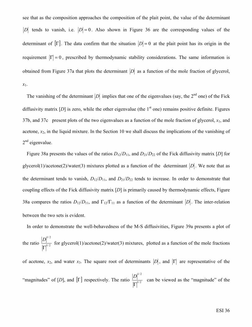
ESI 36

see that as the composition approaches the composition of the plait point, the value of the determinant

D tends to vanish, i.e. 0=D . Also shown in Figure 36 are the corresponding values of the

determinant of [ ]Γ . The data confirm that the situation 0=D at the plait point has its origin in the

requirement 0=Γ , prescribed by thermodynamic stability considerations. The same information is

obtained from Figure 37a that plots the determinant D as a function of the mole fraction of glycerol,

x1.

The vanishing of the determinant D implies that one of the eigenvalues (say, the 2nd one) of the Fick

diffusivity matrix [D] is zero, while the other eigenvalue (the 1st one) remains positive definite. Figures

37b, and 37c present plots of the two eigenvalues as a function of the mole fraction of glycerol, x1, and

acetone, x2, in the liquid mixture. In the Section 10 we shall discuss the implications of the vanishing of

2nd eigenvalue.

Figure 38a presents the values of the ratios D12/D11, and D21/D22 of the Fick diffusivity matrix [D] for

glycerol(1)/acetone(2)/water(3) mixtures plotted as a function of the determinant D . We note that as

the determinant tends to vanish, D12/D11, and D21/D22 tends to increase. In order to demonstrate that

coupling effects of the Fick diffusivity matrix [D] is primarily caused by thermodynamic effects, Figure

38a compares the ratios D12/D11, and Γ12/Γ11 as a function of the determinant D . The inter-relation

between the two sets is evident.

In order to demonstrate the well-behavedness of the M-S diffusivities, Figure 39a presents a plot of

the ratio 2/1

2/1

Γ

D for glycerol(1)/acetone(2)/water(3) mixtures, plotted as a function of the mole fractions

of acetone, x2, and water x3. The square root of determinants D , and Γ are representative of the

“magnitudes” of [D], and [ ]Γ respectively. The ratio 2/1

2/1

Γ

D can be viewed as the “magnitude” of the

ESI 37

Maxwell-Stefan diffusivity in the ternary mixture. The variation of 2/1

2/1

Γ

D appears to be strongly

dependent on the composition of acetone in the mixture. To confirm this, Figure 39b plots 2/1

2/1

Γ

D as a

function of the mole fraction of acetone, x2. We note that the entire data set appears to fall within a

narrow band; these results are analogous to those presented earlier in Figure 5, and Figure 6 for

acetone(1)/benzene(2)/CCl4(3), acetone(1)/benzene(2)/methanol(3), methanol(1)/1-butanol(2)/1-

propanol, acetone(1)/water(2)/1-propanol(3), acetone(1)/1-butanol(2)/1-propanol(3), and 1-

propanol(1)/1-chlorobutane(2)/n-heptane(3) mixtures.

As the second illustration, Figure 40 shows the experimental data for liquid/liquid equilibrium in

water(1)/chloroform(2)/acetic-acid(3) mixtures. The binodal curve is indicated in green. The spinodal

curve is indicated by the red line.

The experimental data of Vitagliano et al.56 for Fick diffusivity matrix [D] of

water(1)/chloroform(2)/acetic-acid(3) mixtures at six different compositions (cf. Figure 40) also

confirm the expectations of Equations (21), and (81). We note that values of the determinant D

progressively decreases in magnitude as the compositions become increasingly poorer in acetic acid. At

the plait point (composition: x1 = 0.375, x2 = 0.261 and x3 = 0.364 ) the matrix of Fick diffusivities

determined by Vitagliano et al.56 by extrapolation of their data is [ ] 1-29 s m10161.037.0

40.092.0 −×

=D . It

can be confirmed that determinant vanishes, i.e. 0=D .

The classic experiments of Vitagliano et al.56 that were published in 1978 were supplemented by more

recent measurements in 2007 by Buzatu et al.57 for Fick diffusivity matrix [D] of

water(1)/chloroform(2)/acetic-acid(3) mixtures at five different compositions; see Figure 41.

The two sets of experimental data of Vitagliano et al.56 and Buzatu et al.57 are combined and analyzed

in Figure 42.

ESI 38

Figure 42a shows a plot of the determinant D as a function of (1 - x3) for

water(1)/chloroform(2)/acetic-acid(3) mixtures. The results show that the determinant D reduces in

magnitude as the compositions approach the two-phase region.

Figure 42b shows a plot of the determinant Γ as a function of (1- x3). As the plait point is

approached, the determinant Γ tends to vanish.

Figure 42c presents a plot of the ratio 2/1

2/1

Γ

D as a function of (1- x3). The square root of determinants

D , and Γ are representative of the “magnitudes” of [D], and [ ]Γ respectively. The ratio 2/1

2/1

Γ

D can be

viewed as the “magnitude” of the Maxwell-Stefan diffusivity in the ternary mixture. The ratio 2/1

2/1

Γ

D

appears to show a simple dependence on the mole fraction of acetone, quite similar to that observed for

the variation of the M-S binary mixtures; see Figure 3.

Figure 42d plots the ratios Γ12/ Γ11, and Γ21/ Γ22 as a function of the determinant Γ . This shows that

the influence of thermodynamic coupling is increased as the spinodal curve is approached.

Figure 42e shows the ratios D12/D11, and D21/D22 of the Fick diffusivity matrix [D] as a function of the

determinant D . We note that as the determinant tends to vanish, D12/D11 increases to values in excess

of unity. The lowering the magnitude of D as the plait point is approached, also signifies an increase in

the importance of coupling effects. It is clear that the coupling effects have their roots in non-ideal

solution thermodynamics.

The data in Figure 38 and Figure 42 lead us to conclude that the condition 0=D implies the

strongest possible diffusional coupling effect.

Clark and Rowley58 report experimental data for the determinant of the Fick diffusivity matrix [D] for

water(1)/2-propanol(2)/cyclohexane(3) mixtures as (T – Tc) where T is the temperature at which the

ESI 39

diffusivities are measured, and critical temperature Tc = 303.67 K; see Figure 43. The elements of the

Fick matrix of diffusivities were measured at a constant composition corresponding to that at the plait

point at 303.67 K: x1 = 0.367, x2= 0.389, x3= 0.244. Examination of the values of the Fick diffusivity

matrix (also indicated in Figure 43a), we see that the coupling effects get increasingly stronger as Tc is

approached; concomitantly the determinant D gets progressively smaller in magnitude.

Figure 44 shows the phase equilibrium diagram for acetone/water/ethylacetate mixtures at 293 K.

Pertler59 reports the values of the elements of the Fick diffusivity matrix in both the ethylacetate-rich

and water-rich regions. In each of these two cases, he adopts a different numbering for the components.

For the ethylacetate-rich region, the values of the Fick diffusivity matrix [D] are reported using the

component number acetone(1)/water(2)/ethylacetate(3); the values are plotted in Figure 44. Particularly

noteworthy is the extremely large negative value of D21. The large negative value of D21 is caused by

the corresponding large negative value of Γ21, as is evident in the plot on the right upper side of Figure

44. We will see in Section 11, that the strong coupling effects engendered by this large negative value

of D21 will leave its imprint on the equilibration trajectory.

Figure 45 presents the experimental data of Pertler59 for the elements of the Fick diffusivity matrix in

the water-rich region of the phase diagram; these values correspond to the component numbering:

acetone(1)/ethylacetate(2)/water(3). The negative value of D12 is caused by the corresponding large

negative value of Γ12, as is evident in the plot on the left upper side of Figure 45.

10. Equilibration trajectories in ternary liquid mixtures

In homogeneous single-phase regions, uphill diffusion can occur as a result of sizable magnitudes of

cross-coefficients of the Fick diffusivity matrix. To demonstrate this let us consider inter-diffusion of

water(1)/chloroform(2)/acetic-acid(3) mixtures that ensues when two different compositions (in the left

and right compartments in Figure 46) are brought in contact. The initial composition of the left

compartment is: x1,L = 0.48, x2,L= 0.1 and x3,L = 0.42. The initial composition of the right compartment

is: x1,R = 0.2, x2,R = 0.38 and x3,R = 0.42. The composition at equilibrium is x1,eq = 0.34, x2,eq = 0.24 and

ESI 40

x3,eq = 0.42. We note that there is no driving force for the transfer of acetic acid, component 3. The

transient equilibration process is described by the coupled two-dimensional matrix equation

−−

−+

++

=

−

LR

LR

RL

RL

xx

xx

DD

DD

t

zerf

xx

xx

x

x

22

11

21

2221

1211

,22

,11

2

1

42

1

2

1 (83)

At the equilibrated composition at equilibrium is x1,eq = 0.34, x2,eq = 0.24 and x3,eq = 0.42, Vitagliano

et al;56 report the Fick diffusivity matrix as

[ ] 2-4181-29 s m10164.0;s m10939.0344.0

368.0309.0 −− ×=×

= DD . For the chosen set of input

parameters, the importance of diffusion couplings can be gauged from the values of

( )( )

( )( ) 367.0;2.1

2222

1121

1111

2212 −=−−−=

−−

LR

LR

LR

LR

xxD

xxD

xxD

xxD; these values indicate that the influence of diffusion

coupling is indeed significant. As a consequence of coupling effects, the equilibration of acetic acid

displays overshoots and undershoots; see Figure 46. In the ternary composition space, the equilibration

trajectory follows a serpentine path, as depicted in the ternary plot in Figure 46.

Serpentine trajectories are also obtained for equilibration in glycerol(1)/acetone(2)/water(3) mixtures;

this is illustrated by the set of two simulations shown in Figure 47.

Let us examine the first of these sets of simulations (for the equilibrium composition x1= 0.1, x2 =

0.432, x3 = 0.468), in more detail in order to gain insights into the phenomena of uphill diffusion. Figure

48a shows the equilibration trajectory in 2D composition (mole fraction) space. The serpentine

trajectory indicates uphill diffusion for glycerol. The uphill transport of glycerol is also clearly evident

when we plot the compositions of each component as a function of the dimensionless distance

coordinate tD

z

ref4 where the value of the chosen reference diffusivity 910−=refD m2 s-1; see Figure

48b. This plot clearly indicates that uphill diffusion is only experienced by glycerol, and not by either

acetone or water. The NRTL parameters describing phase equilibrium for this system are available from

the work of Krishna et al.13 Using the NRTL parameters we determined the activity coefficient, γi, for

ESI 41

each of the component during the transient equilibration process. For each component we determined

the activity, ai,, defined as

iii xa γ= (84)

Figure 48c shows the plot of the activity trajectory in 2D space. The thermodynamic activity shows a

monotonous equilibration trajectory. This is an important result which indicates that glycerol diffusion

is not uphill of its activity driving force. To further strengthen this finding, Figure 48d compares the

profiles of mole fraction and activity, as a function of the dimensionless distance coordinate. The

activity of glycerol does not show any overshoots or undershoots.

It is often true that uphill diffusion in condensed phases is witnessed in composition space; it does not

occur in activity space.

Figure 49a presents the results for the serpentine trajectories obtained with simulations with the

equilibrium composition: x1= 0.18, x2 = 0.22, x3 = 0.6. The same trajectory when plotted in 2D activity

space exhibits a monotonous equilibration; see Figure 49b. The comparison of the transience for

acetone, expressed in both mole fractions and activity plotted against the dimensionless coordinate

tD

z

ref4 is shown in Figure 49c. There is no overshoot or undershoot in the activity profiles for

acetone.

Now let us consider the situation in which initial compositions in the left and right chambers are such

that the equilibrium composition is the plait point of water(1)/chloroform(2)/acetic-acid(3). The initial

composition of the left compartment is: x1,L = 0.5, x2,L = 0.136 and x3,L = 0.364. The initial composition

of the right compartment is: x1,R = 0.25, x2,R = 0.386 and x3,R = 0.364. The average composition is

determined to be x1 = 0.375, x2 = 0.261 and x3 = 0.364, corresponding to the plait point. We note that

there is no driving force for the transfer of acetic acid, component 3. From the data of Vitagliano et al.56

the Fick diffusivity matrix is [ ] 1-29 s m10161.037.0

40.092.0 −×

=D . For the chosen set of input

ESI 42

parameters, we obtain ( )( )

( )( ) 3.2;434.0

2222

1121

1111

2212 −=−−−=

−−

LR

LR

LR

LR

xxD

xxD

xxD

xxD; these values indicate strong

coupling. However, we have a unique situation due to the vanishing of the determinant, 0=D ; one of

the eigenvalues of Fick diffusivity matrix [D] also vanishes. Consequently, the equilibration of all three

components must relax along the eigenvector corresponding to the non-zero eigenvalue

-1291, s m1008.1 −×=eigD ; for more detailed discussions see Krishna et al.60 and Taylor and Krishna.11

The equilibration trajectories are given by the set of uncoupled equations

( ) ( ) 3,2,1;42

1

2

1

1,

=−

−++= ixx

tD

zerfxxx iRiL

eig

iRiLi (85)

These trajectories are linear in the composition space, and do not display any over- or under-shoots

for acetic acid; see Figure 50. It is paradoxical that the composition trajectories are constrained to

follow a linear trajectory despite strong coupling effects.

We now consider published experimental data to verify the serpentine trajectories witnessed in

Figures 46, 47, 48, 49, and 50.

Krishna et al.60 have reported experimental data on the equilibration paths followed in

glycerol(1)/acetone(2)/water(3) mixtures that provide confirmation of curvilinear equilibration

trajectories. In one on the sets of experiments conducted in a Lewis stirred cell, the initial compositions

of the two liquid phases are: Glycerol-rich phase in the bottom cell: x1,0 = 0.85, x2,0 = 0.0,and x3,0 = 0.15;

Acetone-rich phase in the top cell: x1,0 = 0.0, x2,0 = 0.77 and x3,0 = 0.23. The mixture composition ends

up in the region of phase instability; see Figure 51. Consequently, each of the two phases must

equilibrate to the corresponding points at the two ends of the tie-line. The equilibrium compositions at

the end of the tile line are for the Glycerol-rich phase: x1,eq = 0.552, x2,eq = 0.164 and x3,e = 0.284;

Acetone-rich phase: x1,eq = 0.042, x2,eq = 0.894 and x3,eq = 0.064.

In the experiments each of the two equilibration trajectories were monitored experimentally; these are

shown (red circles in the glycerol-rich phase, and green squares in the acetone-rich phase) in Figure 51.

ESI 43

Each of the two phases exhibits one half of a serpentine path. Let us analyze each of the equilibration

paths in more detail.

Krishna et al.60 develop a model to capture the equilibration trajectories that consists of solving a set

of two coupled matrix differential equations in either phase. The solution yields the following relation

−−

−=

−−

0,2,2

0,1,1

2221

1211

2,2

1,1exp

xx

xxt

DD

DD

xx

xx

eq

eq

eq

eq β (86)

where β is the cell constant for the Lewis stirred cell.

The equilibration paths in the glycerol-rich phase are well described by the following values of the

Fick matrix of diffusivities that are obtained by extrapolation of the diffusivity data of Grossmann and

Winkelmann53, 54

[ ] 1-29 s m1035.01.0

04.033.0 −×

=D (87)

The comparison of the experimentally determined equilibration trajectories with the model

calculations for the glycerol-rich phase are shown in in Figure 52. The curvilinear equilibration

trajectory is ascribable to the coupling between species diffusion, evidenced by the non-zero off-

diagonal elements.

For the acetone-rich phase, the comparison of the experimentally determined equilibration trajectories

with the model calculations are shown in Figure 53; here, the model calculations use Fick diffusivity

values using the data of Grossmann and Winkelmann53, 54 for guidance in extrapolation

[ ] 1-29 s m101.11

1.04.2 −×

=D (88)

Figure 54 presents the simulation results for the equilibration trajectory followed in

acetone(1)/ethylacetate(2)/water(3) mixtures when two mixtures of compositions (in mass tractions)

ω1=0.01, ω2=0.01, ω3=0.98, and ω1=0.17, ω2=0.1, ω3=0.73 are allowed to equilibrate to yield the final

equilibrated value ω1=0.09, ω2=0.055, ω3=0.855. The values of the Fick diffusivity used in the

ESI 44

calculations corresponds to the third point in the water-rich data set of Pertler59:

[ ] 1-29 s m10764.0316.0

287.0179.0 −×

−=D . We note that the trajectory followed is serpentine in shape. The

experimental data obtained by Haeberl and Blass61 (shown in the inset to Figure 54) confirms that the

equilibration tends to “hug” the binodal curve rather than follow a straight-line equilibration path.

A unique situation occurs for equilibration near the region of the plait point. The data of Grossmann

and Winkelmann53, 54 when extrapolated to the plait point suggest the set of values

[ ] 0;s m1024.03.0

35.042.0 1-29 =×

= − DD . As a consequence one of the eigenvalues of Fick diffusivity

matrix [D] must vanish and the equilibration of all components must relax along the eigenvector

corresponding to the non-zero eigenvalue -1291, s m1067.0 −×=eigD

( ) ( ) 3,2,1;)exp( 0,,1,, =−−=− ixxtDxx ieqieigieqi β (89)

In the ternary composition space, the trajectory is linear, not serpentine, despite the significant

coupling effects that are implicit in the condition 0=D . The linear trajectory is confirmed by one set

of experimental data of Krishna et al.60 wherein the initial compositions in the two compartments lie on

the tangent to the plait point; the equilibration paths are shown in Figure 55.

11. Spontaneous emulsification, and the Ouzo effect

When the diffusion trajectory in either, or both, of the liquid phases enters the meta-stable region we

may experience spontaneous emulsification,62-64 and the Ouzo effect.65-67 Let us briefly discuss the

Ouzo effect.

The aniseed-based alcoholic beverage variously called Ouzo (in Greece), Anis del Mono (in Spain),

Pastis (in France), Sambuca (in Italy), and Raki (in Turkey), consists of a three component mixture of

ethanol (≈45 vol%), water (55 vol%) and an essential oil called trans-anethol (≈ 0.1%). It is commonly

consumed with the addition of three to five volumes of water to one volume of Ouzo. Figure 56 presents

a phase equilibrium diagram for the ternary mixture of trans-anethol/ethanol/water. Diffusion of water

ESI 45

into the ethanol/trans-anethol phase results in super-saturation of oil phase; the diffusion trajectory leads

into the meta-stable region (in the bottom left corner) in which the oil spontaneously nucleates into tiny

droplets.68 The tiny 1 nm sized droplets scatter light, causing the drink to appear milky white.

For visualization of the Ouzo effect, watch the following videos on YouTube

https://www.youtube.com/watch?v=GxyWncY3O2g

https://www.youtube.com/watch?v=t5jbxh0C0UU

Vitale and Katz67 have coined the generic term “Ouzo effect” to describe such a process of creating

meta-stable liquid-liquid dispersions. Since no input of mechanical energy is involved, this offers an

energy-efficient method of producing nanospheres and nanoparticles.68 The Ouzo effect is distinct from

spinodal decomposition that occurs when the metal-stable state separates into two liquid phases.69

What is the trajectory followed during the equilibration process when water is added to Ouzo? To

answer this question let us zoom in on the bottom left corner of the phase diagram; see Figure 57. In the

classic paper by Ruschak and Miller,63 linear equilibration trajectories are used to predict spontaneous

emulsification. If we assume a linear equilibration process (dashed line), then the binodal envelope is

not penetrated, and no emulsification can occur; see Figure 57. The only possibility that the binodal

envelope can be entered is if the equilibration trajectory follows a curvilinear path. We investigate this

possibility in detail in the following section.

12. Serpentine trajectories, spinodal decomposition, and spontaneous emulsification

Figure 58 depicts the phase equilibrium diagram for the ternary system

toluene(1)/ethanol(2)/water(3). This is one of the systems used by Ruschak and Miller63 to explain the

conditions required for spontaneous emulsification. Consider inter-diffusion of pure water and mixture

of composition E, in the homogenous single phase region. A linear equilibration path (shown by the

dashed line) must necessarily traverse the meta-stable zone that lies between the binodal and spinodal

envelopes. An entry into the meta-stable zone is a pre-requisite to the possible eventuality of

spontaneous emulsification. Consider inter-diffusion of two homogenous mixtures of compositions A

ESI 46

and B, both in the homogeneous region, just above the binodal curve. A linear equilibration process

(shown by the dashed line) shall remain in the homogeneous single-phase region; no spontaneous

emulsification is possible. For A/B inter-diffusion process, if a serpentine trajectory is followed, as

sketched schematically, then the unstable liquid-liquid phase splitting is entered and spinodal

decomposition will occur. Consider inter-diffusion of mixtures of compositions C and D. The linear

equilibration trajectory (shown by the dashed line) is at a tangent to the binodal curve, but remains in

the single-phase region. For C/D inter-diffusion process, a serpentine trajectory will foray into the meta-

stable region and spontaneous emulsification may occur. Since serpentine trajectories are not budgetted

for in the Ruschak-Miller analysis, spontaneous emulsification will be ruled out a priori.

We examine the feasibility of forays into meta-stable regions of the phase diagram by examining the

equilibration trajectories in nine different mixtures:

water(1)/chloroform(2)/acetic-acid(3)

acetone(1)/water(2)/ethylacetate(3)

water(1)/2-propanol(2)/cyclohexane(3)

water(1)/acetone(2)/toluene(3)

toluene(1)/ethanol(2)/water(3)

water(1)/caprolactam(2)/toluene(3)

water(1)/caprolactam(2)/benzene (3)

toluene(1)/propionic-acid (2)/water(3)

ethylacetate(1)/propionic-acid (2)/water(3)

Let us start by examining the diffusion trajectories for water(1)/chloroform(2)/acetic-acid(3) mixtures.

We performed simulations in which the initial composition of the left compartment is: x1,L = 0.55, x2,L =

0.1 and x3,L = 0.35; the initial composition of the right compartment is: x1,R = 0.13, x2,R = 0.38 and x3,R =

0.49. The composition at equilibrium is x1,eq = 0.34, x2,eq = 0.24 and x3,eq = 0.42. The average

composition corresponds to the fifth data set of Vitagliano et al;56 for that reason we take the values of

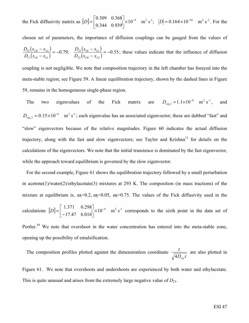
ESI 47

the Fick diffusivity matrix as [ ] 2-4181-29 s m10164.0;s m10939.0344.0

368.0309.0 −− ×=×

= DD . For the

chosen set of parameters, the importance of diffusion couplings can be gauged from the values of

( )( )

( )( ) 55.0;79.0

2222

1121

1111

2212 −=−−−=

−−

LR

LR

LR

LR

xxD

xxD

xxD

xxD; these values indicate that the influence of diffusion

coupling is not negligible. We note that composition trajectory in the left chamber has forayed into the

meta-stable region; see Figure 59. A linear equilibration trajectory, shown by the dashed lines in Figure

59, remains in the homogeneous single-phase region.

The two eigenvalues of the Fick matrix are -1291, s m101.1 −×=eigD , and

-1292, s m1015.0 −×=eigD ; each eigenvalue has an associated eigenvector; these are dubbed “fast” and

“slow” eigenvectors because of the relative magnitudes. Figure 60 indicates the actual diffusion

trajectory, along with the fast and slow eigenvectors; see Taylor and Krishna11 for details on the

calculations of the eigenvectors. We note that the initial transience is dominated by the fast eigenvector,

while the approach toward equilibrium is governed by the slow eigenvector.

For the second example, Figure 61 shows the equilibration trajectory followed by a small perturbation

in acetone(1)/water(2)/ethylacetate(3) mixtures at 293 K. The composition (in mass tractions) of the

mixture at equilibrium is, ω1=0.2, ω2=0.05, ω3=0.75. The values of the Fick diffusivity used in the

calculations [ ] 1-29 s m10016.647.17

298.0371.1 −×

−

=D corresponds to the sixth point in the data set of

Pertler.59 We note that overshoot in the water concentration has entered into the meta-stable zone,

opening up the possibility of emulsification.

The composition profiles plotted against the dimensionless coordinate tD

z

ref4 are also plotted in

Figure 61. We note that overshoots and undershoots are experienced by both water and ethylacetate.

This is quite unusual and arises from the extremely large negative value of D21.

ESI 48

Figure 62 presents the equilibration trajectories in water(1)/2-propanol(2)/cyclohexane(3) mixtures

for the equilibrium composition x1= 0.36, x2 = 0.4, x3 = 0.24, that lies just above the plait point at the

critical temperature Tc = 303.67, i.e. x1 = 0.367, x2= 0.389, x3= 0.244. The equilibration trajectories are

calculated at four different temperatures, 303.75 K, 304.15 K, 304.65 K, 396.65 K. At all four

temperatures, the equilibration trajectories penetrate the binodal curve. The closer the temperature is to

the critical temperature, Tc = 303.67 K, the deeper is the penetration. As a consequence, we should

expect phase splitting should ensue in all the four cases; straight-line equilibration trajectories would

not anticipate phase splitting in any of the four scenarios.

Let us examine the trajectory followed during equilibration of homogenous mixtures of two different

compositions for the system water(1)/acetone(2)/toluene(3). The composition of the equilibrated

mixture is chosen to be x1,eq = 0.2, x2,eq = 0.61 and x3,eq = 0.19, which point lies just above the binodal

curve. The M-S diffusivities of the binary pairs are estimated as

mixturebinary )/toluene(3acetone(2)for ;2;5.0

mixturebinary (3)1)/toluenefor water(;1;5.0

mixturebinary (2)1)/acetonefor water(;3.1;2.5

123

123

113

113

112

112

32

31

21

==

==

==

→→

→→

→→

xx

xx

xx

ÐÐ

ÐÐ

ÐÐ

. At the average composition, the

matrix of thermodynamic factors is calculated from phase equilibrium thermodynamics:

[ ]

−−=Γ

2.1323.0

403.0009.0. Using a combination of equations (35), and (51), we estimate the matrix of

Fick diffusivities [ ] 1-29 s m1038.2574.0

29.119.0 −×

−−=D . It is particularly noteworthy that the Γ11,

and D11 are both negative; thermodynamic stability only requires that the determinants of [ ]Γ and [ ]D

be positive definite. Using this diffusivity estimate, we calculated the diffusion trajectory. We note that

the serpentine trajectory has just not managed to penetrate the binodal envelope; see Figure 63.

As the fifth, and final example we consider inter-diffusion of toluene(1)/ethanol(2)/water(3) mixtures;

the composition (in mole tractions) of the mixture at equilibrium x1,eq = 0.012, x2,eq = 0.208 and x3,eq =

0.78, which point already lies in the meta-stable zone between the binodal and spinodal envelopes. The

M-S diffusivities of the binary pairs are estimated as

ESI 49

mixturebinary /water(3)ethanol(2)for 64.1;7.1

mixturebinary (3)e(1)/waterfor toluen;5.0;0.1

mixturebinary ol(2)e(1)/ethanfor toluen;5.0;0.1

123

123

113

113

112

112

32

31

21

==

==

==

→→

→→

→→

xx

xx

xx

ÐÐ

ÐÐ

ÐÐ

. At the average composition, the

matrix of thermodynamic factors is calculated from phase equilibrium thermodynamics:

[ ]

−

−=Γ

333.0655.1

114.0686.0. Using a combination of equations (35), and (51), we estimate the matrix of

Fick diffusivities [ ] 1-29 s m1053.06.2

1.06.0 −×

−

−=D . Using this diffusivity estimate, we calculated the

diffusion trajectory. We note that the serpentine trajectory has penetrated the spinodal envelope and

entered unstable region; see Figure 64; this implies phase splitting. A further noteworthy point is that

the trajectory in the lower left corner attains negative values for the toluene mole fraction. Therefore, it

is entirely possible that this predicted trajectory is unrealizable in practice.

To set the background for the next two mixtures water(1)/caprolactam(2)/toluene(3) and

water(1)/caprolactam(2)/benzene (3) we shall investigate, we provide the following quote from the PhD

dissertation of Bollen;.70 This dissertation can be downloaded from

http://dissertations.ub.rug.nl/faculties/science/1999/a.m.bollen/ .

The idea that emulsification might be a mass transfer driven process stems from problems in the

industrial extraction of caprolactam from water. Caprolactam is the main feedstock for the manufacture

of nylon-6,6, and there are several processes for its industrial manufacturing. In one of these processes,

which is used by DSM in the Netherlands, the stream leaving the reactor is an aqueous solution of

caprolactam. Caprolactam is extracted from this stream with benzene in a rotating disk contactor

(RDC). In the top of the extraction column, where the reactor stream is fed, a very fine dispersion forms

in the benzene phase, which hinders the separation of the two phases. This, in turn, negatively

influences the purity of the product.

Let us examine the trajectory followed during equilibration of homogenous mixtures of two different

compositions for the system water(1)/caprolactam(2)/toluene(3). The composition of the equilibrated

mixture is chosen to be x1,eq = 0.64, x2,eq = 0.2725 and x3,eq = 0.0875, which point lies on the binodal

ESI 50

curve. At the average composition, the matrix of thermodynamic factors is calculated from phase

equilibrium thermodynamics: [ ]

−−=Γ

10.242.0

52.1176.0. We assume that the matrix of Fick diffusivities is

the product of a scalar diffusivity 10-9 m2 s-1 multiplied by [ ]Γ ; i.e.

[ ] 1-29 s m1010.242.0

52.1176.0 −×

−−=D . Using this estimate, we calculated the equilibration trajectory.

We note that the serpentine trajectory has penetrated the binodal envelope; see Figure 65. This

indicates the spontaneous emulsification is feasible.

Let us examine the trajectory followed during equilibration of homogenous mixtures of two different

compositions for the system water(1)/caprolactam(2)/benzene (3) for the equilibrium composition. The

composition of the equilibrated mixture is chosen to be x1= 0.125, x2 = 0.165, x3 = 0.71 which point lies

on the binodal curve. At the average composition, the matrix of thermodynamic factors is calculated

from phase equilibrium thermodynamics: [ ]

−

−=Γ

11.2878.0

925.0591.0. We assume that the matix of Fick

diffusivities is the product of a scalar diffusivity 10-9 m2 s-1 multiplied by [ ]Γ ; i.e.

[ ] 1-29 s m1011.2878.0

925.0591.0 −×

−

−=D . Using this estimate, we calculated the equilibration trajectory.

We note that the serpentine trajectory has penetrated the binodal envelope; see Figure 66. This indicates

the spontaneous emulsification is feasible.

Let us examine the trajectory followed during equilibration of homogenous mixtures of two different

compositions for the system toluene(1)/propionic-acid (2)/water(3). The composition of the equilibrated

mixture is chosen to be x1,eq = 0.475, x2,eq = 0.4 and x3,eq = 0.285, which point lies on the binodal curve.

At the average composition, the matrix of thermodynamic factors is calculated from phase equilibrium

thermodynamics: [ ]

=Γ

1.19580.1806

0.2963-0.3267. We assume that the matrix of Fick diffusivities is the

product of a scalar diffusivity 10-9 m2 s-1 multiplied by [ ]Γ ; i.e.

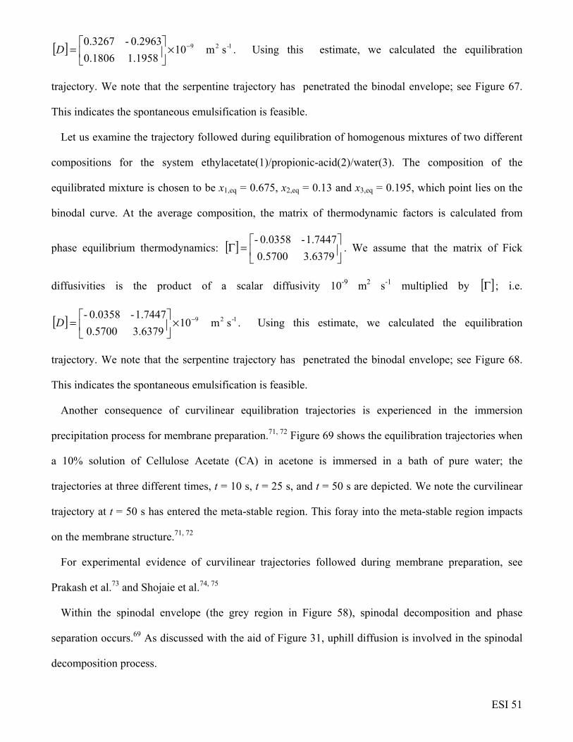
ESI 51

[ ] 1-29 s m101.19580.1806

0.2963-0.3267 −×

=D . Using this estimate, we calculated the equilibration

trajectory. We note that the serpentine trajectory has penetrated the binodal envelope; see Figure 67.

This indicates the spontaneous emulsification is feasible.

Let us examine the trajectory followed during equilibration of homogenous mixtures of two different

compositions for the system ethylacetate(1)/propionic-acid(2)/water(3). The composition of the

equilibrated mixture is chosen to be x1,eq = 0.675, x2,eq = 0.13 and x3,eq = 0.195, which point lies on the

binodal curve. At the average composition, the matrix of thermodynamic factors is calculated from

phase equilibrium thermodynamics: [ ]

=Γ

3.63790.5700

1.7447-0.0358-. We assume that the matrix of Fick

diffusivities is the product of a scalar diffusivity 10-9 m2 s-1 multiplied by [ ]Γ ; i.e.

[ ] 1-29 s m103.63790.5700

1.7447-0.0358- −×

=D . Using this estimate, we calculated the equilibration

trajectory. We note that the serpentine trajectory has penetrated the binodal envelope; see Figure 68.

This indicates the spontaneous emulsification is feasible.

Another consequence of curvilinear equilibration trajectories is experienced in the immersion

precipitation process for membrane preparation.71, 72 Figure 69 shows the equilibration trajectories when

a 10% solution of Cellulose Acetate (CA) in acetone is immersed in a bath of pure water; the

trajectories at three different times, t = 10 s, t = 25 s, and t = 50 s are depicted. We note the curvilinear

trajectory at t = 50 s has entered the meta-stable region. This foray into the meta-stable region impacts

on the membrane structure.71, 72

For experimental evidence of curvilinear trajectories followed during membrane preparation, see

Prakash et al.73 and Shojaie et al.74, 75

Within the spinodal envelope (the grey region in Figure 58), spinodal decomposition and phase

separation occurs.69 As discussed with the aid of Figure 31, uphill diffusion is involved in the spinodal

decomposition process.

ESI 52

13. Aroma retention in drying of food liquids

During drying of food liquids such as orange juice and coffee, it is essential to retain the presence of

volatile aroma compounds whilst removing water. A food liquid typically consists of aroma, water and

sugar or coffee extract. Consider acetone to represent a model aroma compound with malto-dextrin

representing the sugar compound. With decreasing water concentrations there is a strong decrease in the

diffusion coefficients both for acetone and water, with a much stronger decrease of acetone diffusivity;

see Figure 70a. At water concentrations lower than 15 wt % the ratio Dacetone/Dwater becomes so small

that the system can be considered impermeable to acetone; see Figure 70b. In spray drying operation it

is essential to ensure a rapid decrease of water concentration at the outer surface of the food liquid

droplet and if the surface water is very quickly lowered to below 15 wt %, aroma retentions up to 100 %

are possible.76 Rigorous modelling of the drying of food liquids, demands the use of the Maxwell-Stefan

equations (25).

14. Uphill diffusion in mixtures of glasses, metals, and alloys

The proper description of multicomponent diffusion in metals, glasses, steels, alloys, and composites

is important in a wide variety of processes such as bonding, cladding, controlled heat treatments, and

surface modification.77

One of the very first experimental evidence of uphill diffusion is available in the classic experiments

reported by Darken, 17 who was one of the first to recognize the need to use activity gradients as proper

driving forces when setting up the phenomenological relations to describe diffusion The following three

quotes from his 1949 paper also serve as learning points for this tutorial review

“the driving force in an isothermal diffusion process may be regarded as the gradient of the chemical

potential,”,

“for a system with more than two components it is no longer necessarily true that a given element

tends to diffuse toward a region of lower concentration even within a single phase region”, and

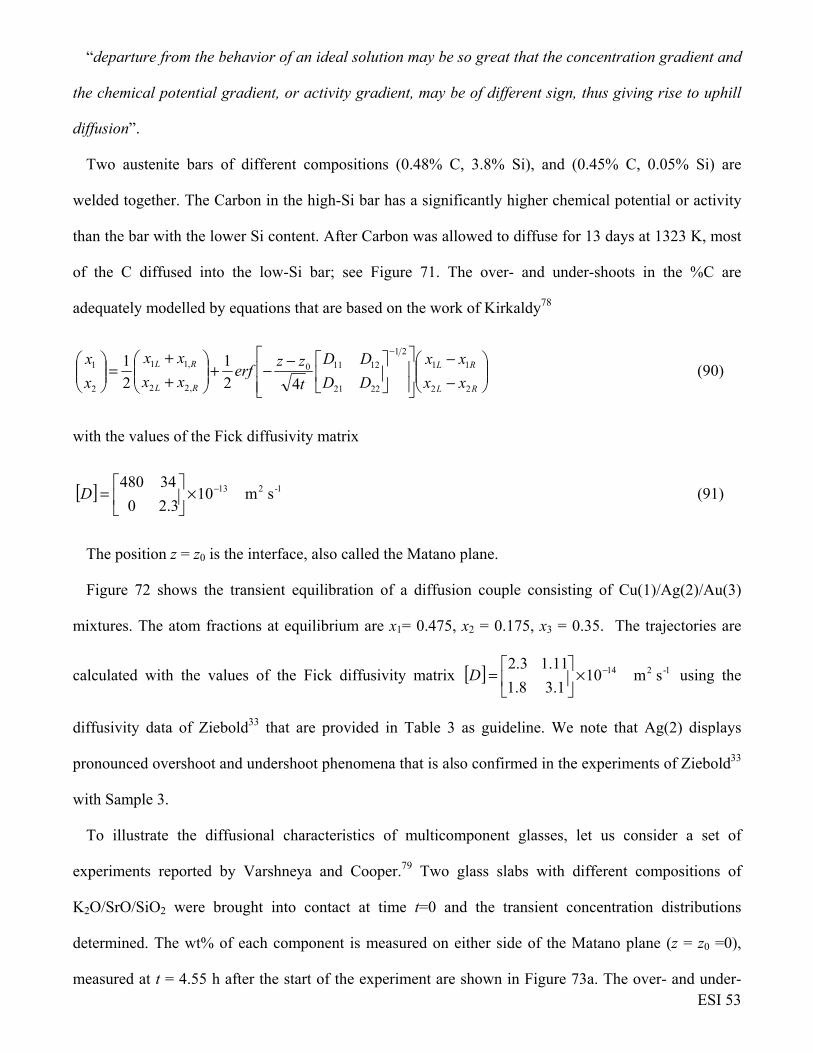
ESI 53

“departure from the behavior of an ideal solution may be so great that the concentration gradient and

the chemical potential gradient, or activity gradient, may be of different sign, thus giving rise to uphill

diffusion”.

Two austenite bars of different compositions (0.48% C, 3.8% Si), and (0.45% C, 0.05% Si) are

welded together. The Carbon in the high-Si bar has a significantly higher chemical potential or activity

than the bar with the lower Si content. After Carbon was allowed to diffuse for 13 days at 1323 K, most

of the C diffused into the low-Si bar; see Figure 71. The over- and under-shoots in the %C are

adequately modelled by equations that are based on the work of Kirkaldy78

−−

−−+

++

=

−

RL

RL

RL

RL

xx

xx

DD

DD

t

zzerf

xx

xx

x

x

22

11

21

2221

12110

,22

,11

2

1

42

1

2

1 (90)

with the values of the Fick diffusivity matrix

[ ] 1-213 s m103.20

34480 −×

=D (91)

The position z = z0 is the interface, also called the Matano plane.

Figure 72 shows the transient equilibration of a diffusion couple consisting of Cu(1)/Ag(2)/Au(3)

mixtures. The atom fractions at equilibrium are x1= 0.475, x2 = 0.175, x3 = 0.35. The trajectories are

calculated with the values of the Fick diffusivity matrix [ ] 1-214 s m101.38.1

11.13.2 −×

=D using the

diffusivity data of Ziebold33 that are provided in Table 3 as guideline. We note that Ag(2) displays

pronounced overshoot and undershoot phenomena that is also confirmed in the experiments of Ziebold33

with Sample 3.

To illustrate the diffusional characteristics of multicomponent glasses, let us consider a set of

experiments reported by Varshneya and Cooper.79 Two glass slabs with different compositions of

K2O/SrO/SiO2 were brought into contact at time t=0 and the transient concentration distributions

determined. The wt% of each component is measured on either side of the Matano plane (z = z0 =0),

measured at t = 4.55 h after the start of the experiment are shown in Figure 73a. The over- and under-

ESI 54

shoots in the SrO concentrations are adequately modelled by equation (90), wherein the matrix of Fick

diffusivities have the values

[ ] 1-213 s m1033.022.1

267.01 −×

−

−=D (92)

Figure 73b shows a 3D trajectory plot of the wt% K2O vs wt% SrO vs wt% SiO2. The equilibration

trajectory is serpentine in shape, and is clearly attributable to the coupled characteristics of the matrix of

Fick diffusivities [ ]D .

If the matrix of Fick diffusivities is assumed to be diagonal with elements

[ ] 1-213 s m1010

01 −×

=D (93)

the corresponding equilibration trajectories are indicated by the dashed lines in Figures 73b. We note

that the transient equilibration becomes monotonic for the uncoupled diffusion process.

Let us examine the experimental data of Vielzeuf and Saúl80 for inter-diffusion of Fe/Mg/Ca mixtures

in garnet, a precious stone consisting of a deep red vitreous silicate mineral. A diffusion “couple” with

two different compositions are brought into contact at time t = 0; see Figure 74. The driving forces for

the three components are (in atom fractions): 14.0;01.0;15.0 321 =Δ=Δ−=Δ xxx . The composition

profiles on either side of the interface marker (z = 0, the Matano plane) are monitored at various time

intervals. The composition profiles at t = 100 h (cf. Figure 74a) shows spatial over- and under-shoot in

the composition profile for Mg, whose driving force is significantly lower than that of the two partner

atoms. In ternary composition space, the equilibration trajectory is serpentine in shape; see Figure 74b.

The modelling of the experimental data Vielzeuf and Saúl80 for inter-diffusion of Fe/Mg/Ca mixtures

in garnet proceeds along similar lines to the foregoing examples. The overshoot in the equilibration of

Mg is adequately modelled using the values of the Fick diffusivity matrix

[ ] 1-219 s m1018.15.5

02.186.5 −×

−

−=D (94)

ESI 55

in equation (90); see Figure 75a. Use of the diagonal matrix

[ ] 1-219 s m1030

03 −×

=D (95)

leads to monotonous equilibration trajectories indicated by the dashed line in Figure 75b.

The non-monotonous equilibration trajectory observed for SrO in Figure 73, and Mg in Figure 75

signal the occurrence of uphill diffusion; such phenomena are of importance in the processing of

ceramics, cements, alloys, steels, and composites.77, 81

For multi-component mixtures ( 3≥n ), uphill diffusion often occurs even when the phase is stable.

Also, the diffusion flux may also be directed uphill, against the chemical potential gradient. In sharp

contrast, in binary systems ( 2=n ), uphill diffusion occurs only in case of phase instability. In binary

systems, diffusion is most commony downhill of the chemical potential, or activity, gradient; it can go

uphill of the concentration gradient in unstable regions.

15. Crossing boundaries in azeotropic distillation

Distillation is the most widely used separation process in the chemical process industries. Design and

simulation procedures for distillation are commonly based on the equilibrium stage model, developed

by Sorel more than a hundred years ago.82 Departures from thermodynamic equilibrium between the

vapor and liquid phases on a distillation tray (see schematic in Figure 76), are commonly accounted for

in practice by introducing the Murphree component efficiencies

niyy

yyE

iEi

iEiLMVi ,...2,1;

*, =−−= (96)

where iEy , and iLy are, respectively, the vapor phase mole fractions, entering and leaving a tray, and *iy

is the vapor composition in thermodynamic equilibrium with the liquid leaving the tray. For a tray in

thermodynamic equilibrium, the component efficiencies are 100% for each component. Mass transfer

resistances on either side of the vapor/liquid interface reduce the component efficiencies to values

below 100%. For binary distillation, the Murhpree component efficiencies are bounded, i.e.

ESI 56

10 ,2,1 ≤=≤ MVMV EE . For multicomponent distillation, with the number of species 3≥n , coupled

diffusion effects in either vapor or liquid phases cause the component efficiencies to be distinctly

different from one another, MVMVMV EEE ,3,2,1 ≠≠ . Phenomena such as osmotic diffusion, diffusion

barrier, and uphill diffusion (cf. Figure 13b) result in Murphree component efficiencies that are

unbounded ( ±∞→MViE , ), zero ( 0, =MViE ), or negative ( 0, <MViE ); this has been demonstrated in

several experimental studies.27, 83-90

Consider distillation of water(1)/ethanol(2)/acetone(3) mixtures. The pure component boiling points

are: water = 373.2 K; ethanol = 351.6 K; acetone = 329.7 K; water/ethanol azeotrope = 351.4 K

(composition of azeotrope = 12% water, 88% ethanol). Ethanol is the component with the intermediate

boiling point. Consequently, the transfer of ethanol is from the liquid to the vapor phase near the top of

the distillation column, approaching the condenser. However, ethanol transfers from the vapor to the

liquid phase near the bottom of the column approaching the reboiler. This implies that the driving force

for transfer of ethanol, ( )Eyy 2*2 − , must necessarily change sign from the bottom to the top of the

column. At some intermediate position, we may also have the situation corresponding to ( ) 02*2 =− Eyy .

In one set of experimental results of Springer et al.84 in the laboratory set-up shown in Figure 77a, the

values of ( )Eyy −*2 are plotted in Figure 77b. We note that the ethanol driving force is negative for

Stages 2 – 9, ( ) 0*2 ≈− Eyy for Stage 10, and ( ) 02

*2 >− Eyy for Stage 11; see Figure 77b. The values of

the MVE ,2 for ethanol is negative on Stage 10; on Stage 11, 1, >MViE ; see Figure 77c. This implies

reverse or uphill diffusion on stages 10 and 11; the transfer of ethanol is dictated by the driving forces

of the other two components ( )Eyy 1*1 − , and ( )Eyy 3

*3 − , that are both finite.84

Unequal component efficiencies, MVMVMV EEE ,3,2,1 ≠≠ , influence the composition trajectories

followed by the vapor and liquid phase along the distillation column. Generally speaking, residue curve

maps provide a good indication of the composition trajectories along the distillation column in which all

the component efficiencies are equal to one another MVMVMV EEE ,3,2,1 == . Figure 78a shows the residue

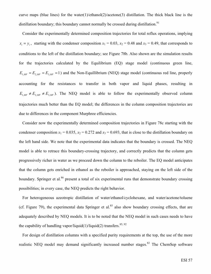
ESI 57

curve maps (blue lines) for the water(1)/ethanol(2)/acetone(3) distillation. The thick black line is the

distillation boundary; this boundary cannot normally be crossed during distillation.91

Consider the experimentally determined composition trajectories for total reflux operations, implying

ii yx = , starting with the condenser composition x1 = 0.03, x2 = 0.48 and x3 = 0.49, that corresponds to

conditions to the left of the distillation boundary; see Figure 78b. Also shown are the simulation results

for the trajectories calculated by the Equilibrium (EQ) stage model (continuous green line,

1,3,2,1 === MVMVMV EEE ) and the Non-Equillibrium (NEQ) stage model (continuous red line, properly

accounting for the resistances to transfer in both vapor and liquid phases, resulting in

MVMVMV EEE ,3,2,1 ≠≠ ). The NEQ model is able to follow the experimentally observed column

trajectories much better than the EQ model; the differences in the column composition trajectories are

due to differences in the component Murphree efficiencies.

Consider now the experimentally determined composition trajectories in Figure 78c starting with the

condenser composition x1 = 0.035, x2 = 0.272 and x3 = 0.693, that is close to the distillation boundary on

the left hand side. We note that the experimental data indicates that the boundary is crossed. The NEQ

model is able to retrace this boundary-crossing trajectory, and correctly predicts that the column gets

progressively richer in water as we proceed down the column to the reboiler. The EQ model anticipates

that the column gets enriched in ethanol as the reboiler is approached, staying on the left side of the

boundary. Springer et al.86 present a total of six experimental runs that demonstrate boundary crossing

possibilities; in every case, the NEQ predicts the right behavior.

For heterogeneous azeotropic distillation of water/ethanol/cyclohexane, and water/acetone/toluene

(cf. Figure 79), the experimental data Springer et al.85 also show boundary crossing effects, that are

adequately described by NEQ models. It is to be noted that the NEQ model in such cases needs to have

the capability of handling vapor/liquid(1)/liquid(2) transfers.85, 92

For design of distillation columns with a specified purity requirements at the top, the use of the more

realistic NEQ model may demand significantly increased number stages.82 The ChemSep software

ESI 58

includes a rigorous implementation the NEQ model for absorption, and distillation processes.82 This

software is available for download at

http://www.chemsep.com/

16. Coupling effects in diffusion of electrolytes

For transport of ionic species in electrolyte solutions, we need to consider the electrostatic potential

gradient as an additional driving force for transport. An important advantage of the M-S formulation is

that the contribution of the electrostatic potential gradient needs to be added to the left member of

equations (25)

niÐc

NxNx

dz

d

RTzx

dz

d

RT

x n

j ijt

jiijii

ii

ij

,2,1;F

1

=−

=Φ−− ≠=

μ (97)

where zi is the charge on species i, and F is the Faraday constant. The species n is usually water (W),

that is usually present in significantly large quantities, and can often be considered stagnant, NW = cW uW

= 0. For dilute aqueous solutions of electrolytes, the ion-ion interactions can often be neglected, and

also dz

dx

dz

d

RT

x iii ≈μ. With these assumptions and simplifications, equations (97) reduce to the Nernst-

Planck equation for the flux of individual ionic species

1,2,1;F −=Φ−−= ni

dz

d

RTÐzc

dz

dcÐN iwii

iiwi (98)

where the Ðiw in equation (98) are the ionic diffusivities. If there is no flow of current, this results in the

electroneutrality constraint

0F1

1

=−

=i

n

ii Nz (99)

Combining equations (98), and (99), we obtain the following expression for the diffusion potential

that is engendered due to ionic diffusion

ESI 59

−

=

−

=−=Φ1

1

2

1

1

F n

iiwii

n

i

iiwi

ÐzcRT

dz

dcÐz

dz

d (100)

The effective diffusivities of ionic species i is

dz

dcdz

d

RTÐzc

Ð

dz

dcN

Di

iwii

iwi

ieffi

Φ

+=−≡

F

, (101)

The diffusion potential has the effect of influencing the motion of each of the ionic species. The

second term on the right of equation (101) serves either to accelerate or decelerate each species,

depending on the species charges, zi, and mobilities.

As illustration, consider the experimental results of Vinograd and McBain93 in a two-compartment

diffusion cell, shown schematically in Figure 80. The bottom compartment contained pure water while

the top one contained an aqueous electrolyte solution. Diffusion takes place through the pores of a

sintered glass disk that separated the two compartments. In one set of experiments, the top compartment

contained an aqueous solution of HCl and BaCl2, the composition of which was varied. On complete

ionization the mixture consists of the ionic species H+, Cl-, Ba2+ and un-ionized H2O. By monitoring

the concentrations of the three ionic species as a function of time, Vinograd and McBain93 obtained the

effective ionic diffusivities Di for H+, Cl- and Ba2+. The experimentally observed ionic diffusivities are

shown in Figure 80 as function of the square root of the ratio of the initial ionic concentrations of H+

and Ba2+ in the top compartment ++ Ba2H cc . With increasing values of ++ Ba2H cc , it is observed that

both DH+ and DBa2+ decrease while DCl- increases. During the start of the diffusion process, the highly

mobile H+ diffuses ahead of its companion ions into the pure water compartment, creating an excess of

positive charge. This induces a diffusion potential dzdΦ which acts in such a way as to maintain

electro-neutrality. The consequence is that the Cl- experiences an extra electrostatic “pull”, enhancing

its effective diffusivity value. The electrical potential gradient also serves to retard the motion of the

positive ions H+ and Ba2+ or in other words these ions experience a “push” in a direction opposite to that

ESI 60

dictated by their composition gradient driving forces. For ++ Ba2H cc =2 the electrostatic “push” on

Ba2+ is such as to result in a vanishing value for DBa2+. The continuous solid lines in Figure 80 are the

calculations of the effective diffusivities according to equation (101); further computational details are

provided in Example 2.4.2 of Taylor and Krishna.11 For ++ Ba2H cc > 2, negative values of DBa2+ are

obtained, signifying that uphill diffusion is feasible.

It should also be clear from Equation (100) that the sign of diffusion potential is dictated by the

concentration gradients of the individual ions and is therefore dependent on the signs (i.e. directions) of

the concentration gradients. This directional influence of the diffusion potential is illustrated clearly by

the experiments of Kraaijeveld and Wesselingh94 for external mass transfer limited ion exchange.

Exchanging Na+ within the ion exchange bead with H+ from the bulk chloride solution proceeds at a

significantly higher rate than for the reverse exchange process; see Figure 81. Analogous asymmetric

exchange kinetics is found for the Ca2+/H+/Cl- system.94 The details of the modelling of diffusion in ion-

exchange processes is available in Wesselingh and Krishna.25

Yang and Pintauro95 report an interesting set of experimental data for transient transport of H+, Na+,

and Cs+ ions across a Nafion cation exchange membrane separating the acid and salt compartments; see

Figure 82. The HSO4- and SO4

2- ions cannot cross the membrane. The H+ ions transfer from the acid to

the salt compartment. Both Na+, and Cs+ ions transfer from the salt to the acid compartment. Due to the

significantly higher mobility of the H+ ions, there is a significant influence of the diffusion potential

dz

dΦ that tends to accelerate the motion of the Na+, and Cs+ ions during the initial stages of the

transience. Since the concentration driving force of Cs+ ions is very small, the initial transience is

strongly dictated by the diffusion potential dz

dΦ; this results in the observed overshoot in the transient

equilibration of Cs+.

ESI 61

17. Reverse osmosis

The best known example of uphill diffusion is in the reverse osmosis (RO) process for desalination in

which fresh water is recovered from saline water by use of a polyamide film membrane that rejects salt,

and only allows water to permeate; see Figure 83. The transport of water occurs from the compartment

with salt water (typically 98% water), on the left of the membrane to a region with nearly 100% pure

water, on the right side. Uphill transport of water is achieved by application of a pressure differential

across the membrane that must exceed the osmotic pressure of 2.7 MPa.25 Both concentration and

pressure gradients dictate the net flux of water across the RO membrane; equation (2) does not provide

an adequate description of inter-membrane transport.

In reverse osmosis, the driving force for transport across the polyamide membrane layer must

additionally account for the contribution of the pressure gradients. The expression for the flux of water

across the membrane (see schematic in Figure 83) is obtained by modifying equation (25) as follows

wMt

ww

ww

Ðc

N

dz

dpV

RTdz

d

RT

x =−− 1μ (102)

where wV is the partial molar volume. In equation (102), we ignore diffusional interactions between

water and salt. Furthermore, ignoring thermodynamic non-ideality effects, we can re-write Equation

(102) in the following form for a membrane of thickness δ

wMt

ww

w

Ðc

NpV

RT

x =Δ−Δ−δδ

1 (103)

In desalination operations, the upstream compartment will typically have 2 mole % salt and the

downstream compartment will be practically salt-free. Therefore, the driving force for water transport

02.098.00.1 =−=Δ wx . If no additional pressure is applied to the upstream compartment, the pressure

difference at equilibrium, corresponding to 0=wN , is called the osmotic pressure

w

w

V

xRTp

Δ−=Π=Δ (104)

ESI 62

Typically, T = 298 K, and 5108.1 −×=wV m3 mol-1; the osmotic pressure is 2.75 MPa. In order to

drive water from the left to right in Figure 83, we need to apply pΔ values exceeding 2.75 MPa. In

desalination operations we have uphill diffusion of water by application of an additional driving force.

Further details on the modelling of transport phenomena in reverse osmosis is provided by Wesselingh

and Krishna.25

In electro-osmosis, water is dragged uphill by electrostatic potential gradients; see Wesselingh and

Krishna.25

18. The Soret Effect

The Soret effect, also called thermal diffusion, is the tendency of a mixture of two or more

components to separate due to a temperature gradient. In 1879 Charles Soret discovered that a salt

solution contained in a tube with the two ends at different temperatures did not remain uniform in

composition; the salt was more concentrated near the cold end than near the hot end of the tube; for a

review of the history and applications see Platten.96

One usually writes for the mass flux of the reference chemical compound in a binary mixture

( )dz

dTD

dz

dDJ Ttt 11

1121 1 ωωρωρ −−−= (105)

The first term in the right hand side of Equation (105) is Fick’s law of diffusion, with the mass

fraction 1ω of the reference component 1 and D12 the Fick diffusivity; the second term describes the

Soret effect or thermo-diffusion effect, proportional to the temperature gradient dz

dT, with DT the

thermo-diffusion coefficient. Since the thermo-diffusion effect does not exist in pure fluids one, the

factor ( )11 1 ωω − is included in the right member of Equation (105). Even so, DT remains concentration

dependent, exactly as the Fick diffusivity D12. Thus the second term in the right hand side of Equation

(105) describes mass separation due to a temperature gradient, whereas the first describes

ESI 63

homogenization by Fickian diffusion. The two terms are thus of opposite sign, and when they are of

equal intensity, we are in steady-state conditions

( ) 01 111

121 =−−−=dz

dTD

dz

dDJ Ttt ωωρωρ (106)

implying

( )dz

dT

D

D

dz

d T11

12

1 1 ωωω −−= (107)

and the Soret coefficient ST is defined as

( )dz

dTdz

d

D

DS T

T

1

11 1

1ω

ωω −−== (108)

The Soret coefficient ST may be positive or negative depending on the sign of DT or on the sense of

migration of the reference component 1 to the cold or to the hot regions. In absolute value an order of

magnitude for usual organic mixtures or aqueous solutions is ST = 0.001 to 0.01 K−1. Typically, the

value of the mass fraction difference between the hot and cold ends 01.01 ≈Δω , often smaller. But even

if the separation remains small, the Soret effect has some practical implications. For example, Huang et

al.97 demonstrate the use of thermal diffusion for fractionation of isotopes of Fe, Ca, and Mg from

silicate melts.

Coupling between the salinity and temperature gradients often cause double-diffusive convection, and

salt fingers that are of importance in oceanography and geology.98

19. Separations using micro-porous crystalline materials: General considerations

A wide variety of ordered crystalline porous materials is used in several applications in separation

applications.99-102 These include zeolites (crystalline aluminosilicates), carbon nanotubes (CNTs),

metal-organic frameworks (MOFs), zeolitic imidazolate frameworks (ZIFs), covalent organic

ESI 64

frameworks (COFs), periodic mesoporous organosilicas organosilicas (PMOs), SBA-16, and MCM-41.

The characteristic pore dimensions of these structures are either in the micro-porous (dp < 2 nm), or

meso-porous ranges (2 nm < dp < 50 nm). The main focus of our attention will be on micro-porous

crystalline materials.

A number of different channel topologies and connectivities are encountered in zeolites, MOFs,

COFs, and ZIFs; these can be divided into five broad classes;

1. One-dimensional (1D) channels (e.g. AFI, LTL, TON, Fe2(BDP)3, MgMOF-74, MIL-47,

MIL-53(Cr), BTP-COF); see Figure 84.

2. 1D channels with side pockets (e.g. MOR, FER); see Figure 85.

3. Intersecting channels (e.g. MFI, BEA, BOG, Zn(bdc)dabco, Co(bdc)dabco); see Figure 86.

4. Cages separated by narrow windows (e.g. LTA, CHA, DDR, ZIF-8); see Figure 87.

5. Cavities with large windows (e.g. FAU, IRMOF-1, CuBTC, MOF-177); see Figure 88.

Further details on the structure, landscape, pore dimensions on a very wide variety of micro-porous

materials are available in the published literature.103-105

The technologies used in industrial separations are either pressure swing adsorption (PSA) units

(exemplified in Figure 89), or membrane permeation devices (see schematic in Figure 90).

The operations of fixed bed adsorption units are intrinsically transient in nature, i.e. the gas (or fluid)

phase concentrations vary both with distance along the adsorber, z, and time, t.104, 106-108 Most

commonly, the separation performance of PSA adsorbers is dictated by mixture adsorption equilibrium.

Intra-particle diffusion limitations cause distended breakthrough characteristics and usually lead to

diminished separation effectiveness. There are however some examples, as we shall examine later,

where diffusional influences act in a manner so as to enhance separations. At the other extreme, we

could have a situation in which diffusional effects over-ride the influence of adsorption equilibrium and

is the prime driver for separation. For separation of O2(1) /N2(2) mixture using LTA-4A, LTA-5A, or

NaX, the adsorption selectivity is in favor of N2 due to the larger permanent quadrupole of N2 compared

to that of O2. This implies that an adsorption based process would selectively adsorb N2, and pure O2

ESI 65

can be produced in the adsorption phase of PSA operations.109, 110 For production of purified N2, it is

desirable to selectively adsorb O2. This selectivity towards O2 can be achieved by choosing LTA-4A

zeolite. Diffusion limitations are severe in LTA-4A because the window regions are partially blocked

by the cations (see Na+ locations in the window regions shown in Figure 89). Due to its smaller cross-

sectional dimension, 3.1 Å for O2, compared to 3.3 Å for N2, the inter-cage hopping of O2 occurs at a

rate that is about 100 times higher than that of N2. The significantly lower diffusivity of N2 has the

consequence that purified N2 breaks through earlier in a fixed bed adsorber; see simulated

breakthroughs in Figure 89.

By contrast to PSA units, the separation performance of membrane devices (see schematic in Figure

90) is always influenced by intra-crystalline diffusion, in addition to adsorption equilibrium.111, 112

We now examine the modelling of intra-crystalline diffusion, and the significance of coupling effects.

20. Fick, Onsager, and Maxwell-Stefan formulations for diffusion inside micro-porous crystalline materials

In contrast to the treatment of diffusion in bulk fluid mixtures for which the reference frame is chosen

as the molar average velocity of the mixture (cf. Equation (4)), the molar fluxes for diffusion in

microporous crystalline materials are defined with respect to the material framework, i.e. Ni = Ji.29, 107 In

development of flux relations it is tacitly assumed that the framework material is the (n+1)th component

of the mixture. Unary diffusion inside the pores is comparable in characteristics to diffusion in binary

fluid mixtures. Put another way, the “dimensionality” of the diffusion is increased by unity when we

write the flux relations for diffusion inside pores. Binary mixture diffusion in microporous materials is

described by 2 × 2 dimensional matrix equations, much in the same way as bulk liquid phase diffusion

in ternary mixtures.

For unary diffusion, the Fickian formulation relates the component flux Ni, expressed as the number

of moles of species i transported per m2 surface of crystalline material per second, to the gradient of the

molar loadings, qi

ESI 66

dz

dqDN i

ii ρ−= (109)

where ρ is the framework density. Equation (109) defines the Fick diffusivity Di, also termed

“transport” diffusivity.99 The Fick diffusivity Di can be determined by fitting transient uptake data and

from chromatographic experiments.113

For a binary mixture consisting of species 1 and 2, each of the component fluxes N1 and N2, is

influenced by the gradients in the molar loadings, dz

dq1 , and dz

dq2 of both species in the mixture. In the

Fick formulation for binary mixtures, diffusion coupling effects are accounted for by defining a matrix

of Fick diffusivities

2221

1211

DD

DD:

nformulatioFick ;2

1

2221

1211

2

1

−=

dz

dqdz

dq

DD

DD

N

Nρ (110)

A major shortcoming of the Fickian formulation (110) is that the diagonal elements of

2221

1211

DD

DD

cannot be related simply to the data for unary Fick diffusivities of components 1 and 2, i.e. D1 and D2.

The ratios 1112 DD , and 2221 DD reflect the extent of “coupling” in the species fluxes. Such couplings

have two different origins, and to distinguish between these it is necessary to adopt the Maxwell-Stefan

mixture diffusion formulations that use chemical potential gradients, dz

d 1μ and

dz

d 2μ, are used as

driving forces of intra-crystalline diffusion.

In the Onsager formulation, the fluxes are linearly related to the chemical potential gradients by

defining a matrix of Onsager coefficients [L]

nformulatioOnsager ; 2

1

2221

1211

2

1

−=

dz

ddz

d

LL

LL

RTN

Nμ

μρ

(111)

ESI 67

The Onsager Reciprocal Relations29 prescribes the symmetry relation

2112 LL = (112)

The Onsager formulation suffers from the major disadvantage that the diagonal elements L11 and L22

cannot be identified with the corresponding values L1, and L2 for unary transport of species 1 and 2.29

The most convenient formulation for diffusion inside porous materials is afforded by the Maxwell-

Stefan (M-S) equations, which for n-component diffusion inside micro-porous crystalline can be written

as29, 103, 105, 114-116

niÐ

N

Ð

NxNx

dz

d

RT

q n

j i

i

ij

jiijii

ij

,..2,1;1

=+−

=− ≠=

μρ (113)

where qi are molar loadings of the adsorbed species. The fluxes Ni defined in Equations (113) are

expressed in terms of the number of moles of species i transported per m2 of the surface of material per

second.

In Equations (113) the Ði is the M-S diffusivities of species i, portraying the interaction between

component i in the mixture with the surface, or wall of the structure. An important advantage of the M-S

formulation is that Ði can be identified with the values for unary species i; there are however

exceptional circumstances where this advantage does not hold.117, 118

The xi in Equations (113) represent the component mole fractions in the adsorbed phase within the

pores and calculated from

nqqx tii ,.....2,1;/= (114)

where qt is the total mixture loading:

=

=n

iit qq

1

(115)

The Ðij are M-S exchange coefficients representing interaction between component i with component

j. At the molecular level, the Ðij reflect how the facility for transport of species i correlates with that of

ESI 68

species j. For micro-porous crystalline materials, the magnitudes of Ðij are a fraction of the

corresponding M-S diffusivity for the binary fluid mixture.21, 111, 119 The stronger the degree of

confinement within the pores, the lower is the fraction. For meso-porous materials the guest molecules

are not strongly constrained and, as a consequence, the Ðij can be identified with that of the diffusivity

of the binary fluid mixture of the pair i-j.21, 111, 119 Indeed, for mesoporous materials, Equations (113)

are essentially equivalent to the Dusty Gas Model (DGM).120 In the DGM, the Ði are calculated with the

help of the Knudsen formula, but the limitations of this assumption for strongly adsorbing species has

been underscored in several recent investigations.118, 121, 122

The Onsager reciprocal relations prescribe the symmetry constraint

jiij ÐÐ = (116)

By defining an n-dimensional square matrix [B] with elements

njiÐ

xB

Ð

x

ÐB

ij

iij

n

j ij

j

iii

ij

....2,1,;;1

1

=−=+= ≠=

(117)

we can recast equation (113) into the following form

niNBdz

d

RT

q n

jjij

ii ,..2,1;1

==− =

μρ (118)

The chemical potential gradients dzd iμ can be related to the gradients of the molar loadings, qi, by

defining thermodynamic correction factors Γij

njiq

f

f

q

dz

dq

dz

fdq

dz

d

RT

q

j

i

i

iij

n

j

jij

ii

ii ,....1,;;ln

1

=∂=ΓΓ== = ∂

μ (119)

Let us now examine the two special cases of unary and binary systems.

For unary diffusion of component i, the Maxwell-Stefan relations simplify to yield

systemunary ;;i

i

i

ii

iii

iii q

f

f

q

dz

dqÐ

dz

dqDN

∂∂ρρ =ΓΓ−=−= (120)

ESI 69

where the commonly used Fick diffusivity of species i is related to the unary Maxwell-Stefan diffusivity

systemunary ;iii ÐD Γ= (121)

The influence of the thermodynamic correction factor is analogous to that for binary diffusion in fluid

mixtures; cf. equation (43). If the adsorption isotherm is described by a single-site Langmuir isotherm,

the thermodynamic factor is

isothermLangmuir site-single;1

1

−

=Γi

i θ (122)

Figure 91a presents a calculation of the thermodynamic factor Γi, for single-site Langmuir isotherm,

plotted as a function of the fractional occupancy, iθ . The thermodynamic factor iΓ always exceeds

unity and we have the hierarchy ii ÐD ≥ . At pore saturation, we have ∞→Γ→ ii ;1θ , and it is

therefore convenient to calculate the inverse thermodynamic factor iΓ1 which decreases linearly with

iθ ; see Figure 91b.

The thermodynamic factor iΓ has a direct influence on the transient adsorption/desorption processes.

During the adsorption phase, the influence of increasing iΓ is to accelerate the component uptake.

However, during the desorption phase, iΓ decreases progressively, and the process becomes

progressively slower. One of the first studies to demonstrate the asymmetry in the adsorption and

desorption kinetics was that of Garg and Ruthven123 for C2H6 in LTA-4A. They showed that desorption

is a slower process than transient uptake; for a quantitative analysis of the experimental data of Garg

and Ruthven;123 see the simulations presented in the Supporting Material accompanying the paper by

Krishna.104

For transient unary uptake within a crystal, the radial distribution of molar loadings, qi, within a

spherical crystallite, of radius rc, is obtained from a solution of a set of differential equations describing

the uptake

ESI 70

( )ii Nr

rrt

trq 22

11),(

∂∂−=

∂∂

ρ (123)

At any time t, during the transient approach to thermodynamic equilibrium, the spatially averaged

molar loading within the crystallite rc is obtained by integration of the radial loading profile

drrtrqr

tqcr

ic

i2

03),(

3)( = (124)

The )(tqi can be compared directly with experimental transient uptake data. An analytical solution to

equation (123) is only possible for the special case in which the Fick Di can be considered to be

independent of the loading. In this case, the expression for fractional approach to equilibrium is113

( )

( ) ∞

=

−−=

−∞=−

12

222

2

)exp(6

1)0,(),(

)0,()(

m

c

i

cici

cii

m

tr

Dm

rqtrq

rqtqπ

π (125)

Equation (125) allows data on transient uptake to be fitted to obtain an average value of the Fick

diffusivity Di that is representative of the range of loadings encountered in the experiment.

Figure 92 shows the experimental data for transient adsorption and desorption profiles for C2H6 in

LTA-4A zeolite. The adsorption branch can be fitted with 2ci rD = 1.1×10-3 s-1, while the desorption

branch yields a lower value 2ci rD = 6×10-4 s-1. The asymmetry in the adsorption and desorption

kinetics is not easy to interpret on the basis of the Fick formulation.

The inverse thermodynamic factor, iΓ1 , decreases linearly with fractional occupancy (cf. Figure

91b). Both the adsorption and desorption cycles can be fitted with 2ci rÐ = 2×10-4 s-1. This implies that

that the asymmetry in the adsorption and desorption transience has their origin in the characteristics of

iΓ1 ; the slower desorption kinetics is attributable to the decrease in iΓ during the desorption phase.

Experimental data of Niessen and Karge124 for transient adsorption/desorption of p-xylene in MFI

zeolite (H-ZSM-5) at 375 K are shown in Figure 93. Niessen and Karge124 found that data for the

desorption phase could be fitted with a Fick diffusivity that is a factor 16 lower than the fitted

ESI 71

diffusivity for the adsorption phase. The differences in the diffusivities are easy to rationalize by the

Maxwell-Stefan equations, and the influence of the thermodynamic correction factor iΓ .

There are many cases, however, in which the simple Langmuir isotherm model does not adequately

capture the isotherm characteristics. For the adsorption of methanol and ethanol in ZIF-8, for example,

the adsorption isotherms (cf. Figure 94a) show steep characteristics.117 The steepness of the isotherms

can only be properly captured by using the dual-site Langmuir-Freundlich isotherm

Bi

Bi

Ai

Ai

iBi

iBisatBi

iAi

iAisatAii

fb

fbq

fb

fbqq

,

,

,

,

,

,,,

,

,,,

11 ν

ν

ν

ν

++

+= (126)

with at least one of the exponents iν exceeds unity; the fits are shown by the continuous solid lines.

Analytic differentiation of equation (126) yields iΓ . As saturation is approached ∞→Γi , and so it is

much more convenient to plot the inverse thermodynamic factor, iΓ

1 as a function of the loading; see

Figure 94b. We note that the iΓ

1 exceeds unity for a range of loadings; this signifies the molecular

clustering effects.117, 125-129 Such effects are akin to the steep decrease in the thermodynamic factors

observed for methanol/n-hexane mixtures in the composition range corresponding to liquid-liquid phase

splitting; cf. Figures 25, and 26.

For the range of loadings in which 11 >Γi

, the Fick diffusivity is lower than the M-S diffusivity, i.e.

ii ÐD ≤ . This trend is confirmed by the experimental data of Chmelik et al.130 for the unary Fick and

M-S diffusivities of methanol, and ethanol in ZIF-8; see Figures 94c, and 94d.

For a binary mixture, the Maxwell-Stefan diffusion equations are29, 103, 105, 114-116

2

2

12

122122

1

1

12

211211 ;

Ð

N

Ð

NxNx

dz

d

RT

q

Ð

N

Ð

NxNx

dz

d

RT

q

+−=−

+−=−

μρ

μρ (127)

ESI 72

For a binary mixture, the chemical potential gradients can be related to the gradients in molar loadings

Γ+Γ

Γ+Γ=

ΓΓΓΓ

=

dz

dq

dz

dqdz

dq

dz

dq

dz

dqdz

dq

dz

dq

dz

dq

RT 222

121

212

111

2

1

2221

1211

22

111

μ

μ

(128)

The elements Γij can be determined from models describing mixture adsorption equilibrium, relating

the component molar loadings q1 and q2, to the partial gas phase fugacities f1 and f2. The off-diagonal

elements of the matrix

ΓΓΓΓ

2121

1211 can have magnitudes significantly larger than unity.

For the simple case in which each species is described by a single-site Langmuir isotherm for either

component in the binary mixture

isothermLangmuir component -single;1

,

ii

iisatii fb

fbqq

+= (129)

the partial gas phase fugacities are related to the component loadings by the mixed-gas Langmuir

model:

Langmuir gas-mixed;2,1;1 2211,

=++

== ifbfb

fb

q

q iii

sati

i θ (130)

Differentiation of equation (130) yields

modelLangmuir gas-mixed;1

1

1

1

12,1

,2

1,2

,12

212221

1211

−

−

−−=

ΓΓΓΓ

θθ

θθ

θθsat

sat

sat

sat

q

qq

q

(131)

While, the mixed-gas Langmuir model is commonly used for describing mixture adsorption; in the

more general case we need to use the Ideal Adsorbed Solution Theory (IAST) developed by Myers and

Prausnitz.131 Equation (131) also implies that the

ΓΓΓΓ

2121

1211 reduces to the identity matrix at low

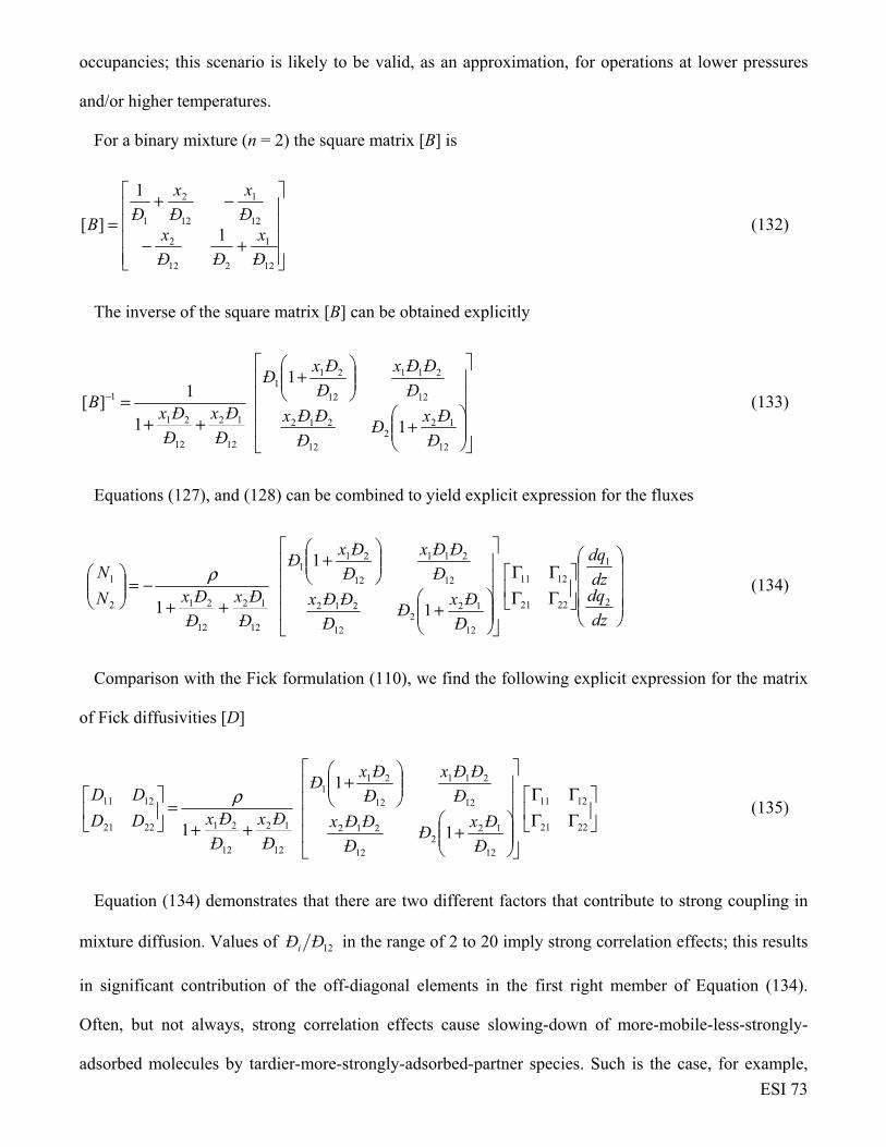
ESI 73

occupancies; this scenario is likely to be valid, as an approximation, for operations at lower pressures

and/or higher temperatures.

For a binary mixture (n = 2) the square matrix [B] is

+−

−+=

12

1

212

2

12

1

12

2

1

1

1

][

Ð

x

ÐÐ

xÐ

x

Ð

x

ÐB (132)

The inverse of the square matrix [B] can be obtained explicitly

+

+

++=−

12

122

12

212

12

211

12

211

12

12

12

21

1

1

1

1

1][

Ð

ÐxÐ

Ð

ÐÐx

Ð

ÐÐx

Ð

ÐxÐ

Ð

Ðx

Ð

ÐxB (133)

Equations (127), and (128) can be combined to yield explicit expression for the fluxes

ΓΓΓΓ

+

+

++−=

dz

dqdz

dq

Ð

ÐxÐ

Ð

ÐÐx

Ð

ÐÐx

Ð

ÐxÐ

Ð

Ðx

Ð

ÐxN

N

2

1

2221

1211

12

122

12

212

12

211

12

211

12

12

12

212

1

1

1

1

ρ (134)

Comparison with the Fick formulation (110), we find the following explicit expression for the matrix

of Fick diffusivities [D]

ΓΓΓΓ

+

+

++=

2221

1211

12

122

12

212

12

211

12

211

12

12

12

212221

1211

1

1

1Ð

ÐxÐ

Ð

ÐÐx

Ð

ÐÐx

Ð

ÐxÐ

Ð

Ðx

Ð

ÐxDD

DD ρ (135)

Equation (134) demonstrates that there are two different factors that contribute to strong coupling in

mixture diffusion. Values of 12ÐÐi in the range of 2 to 20 imply strong correlation effects; this results

in significant contribution of the off-diagonal elements in the first right member of Equation (134).

Often, but not always, strong correlation effects cause slowing-down of more-mobile-less-strongly-

adsorbed molecules by tardier-more-strongly-adsorbed-partner species. Such is the case, for example,

ESI 74

for diffusion of CO2/H2 mixtures in structures as MgMOF-74 and NaX zeolite.111 Correlation effects

generally act to reduce the propensity for overshoots, and uphill diffusion.

Values of 12ÐÐi << 1, imply negligible influence of correlations; in this case, the first members on

the right of Equations (127) can be ignored, yielding

nscorrelatio negligible;0

0

2

1

2221

1211

2

1

2

1

ΓΓΓΓ

−=

dz

dqdz

dq

Ð

Ð

N

Nρ (136)

Extensive Molecular Dynamics (MD) simulations have shown that correlation effects are of

negligible importance for mixture diffusion across cage type zeolites such as ZIF-8, CHA, LTA, DDR,

ERI that consist of cages separated by windows in the 3.4 Å – 4.2 Å size range;103, 105, 111, 132 molecules

jump one-at-a-time across the narrow windows, and the assumption of negligible correlations is

justified. Indeed, in all the analyses presented below, we use equations (136) to model overshoots in

transient binary mixture diffusion.

21. Overshoots in transient uptake of binary mixtures in microporous materials

Let us begin by considering the separation of N2(1)/CH4(2) mixtures that is important in the context of

natural gas upgrading. For transportation purposes, the pipeline specifications usually demand that the

amount of N2 in natural gas is less than about 3%, because the presence of N2 reduces the heating value.

For purification of natural gas streams, that is commonly available at high pressures, it is desirable to

use adsorbents in pressure swing adsorption (PSA) units that are selective to N2 that is present in

quantities that are often as high as 20%. For most known adsorbents, the adsorption selectivity favors

CH4. One practical solution to this problem is to rely on diffusion selectivities by using microporous

materials that have significantly higher diffusivities of N2, compared to that of CH4.133, 134

The earliest study demonstrating the possibility of utilizing diffusion selectivities for separating

N2(1)/CH4(2) mixtures is contained in the classic paper of Habgood135 that presents experimental data

on transient uptake of N2(1)/CH4(2) mixtures in crystallites of LTA-4A. His data measured at 194 K

ESI 75

with partial pressures p1 =50.9 kPa and p2 =49.1 kPa are shown in Figure 95. The N2(1)/CH4(2) mixture

constitutes a combination of more-mobile-less-strongly-adsorbed-N2 and tardier-more-strongly-

adsorbed-CH4. Nitrogen is a “pencil-like” molecule (4.4 Å × 3.3 Å) that can hop length-wise across the

narrow windows; the “spherical” CH4 (3.7 Å) is much more severely constrained and has a diffusivity

that is 22 times lower than that of N2. But N2 has an adsorption strength that is a factor 2.2 lower than

that of CH4. During the initial stages of the transient uptake, the pores of LTA-4A are predominantly

richer in the more mobile N2, but this is displaced by the more strongly-adsorbed-but-tardier CH4

molecules at longer times. This results in an overshoot in the N2 uptake in the experimental data. Note

that the maximum loading of N2 is about a factor 2.5 times that of the final equilibrated uptake. Put

another way, supra-equilibrium loadings are attained for N2 during a short time interval in the early

stages of the transient uptake.

Based on his experimental results for transient uptake, Habgood filed a patent claiming that natural

gas could be upgraded by removing the faster diffusing nitrogen using 4A zeolite and a kinetically

controlled separation process at a low sub-ambient temperature.

Let us now model the transient uptake process. The windows separating adjacent cages of LTA-4A

zeolite are about 4 Å in size; each of the constituent species hops across the windows one-at-a-time. Put

another way, the jumps are not correlated, and equations (136) can be used to describe intra-crystalline

diffusion within crystals.

The calculations of the elements of the matrix of thermodynamic factors Γij for N2(1)/CH4(2) mixture

within LTA-4A crystals demonstrate the significance of the off-diagonal elements at higher loadings;

see Figure 96a. We note that for total mixture loadings, qt = q1+ q2 less than 0.5 mol kg-1, the off-

diagonal elements of the matrix

ΓΓΓΓ

2121

1211 are less than about 0.1. However, for qt > 1.5 mol kg-1, the

off-diagonal elements approach values close to that of the diagonal elements. In other words,

thermodynamic coupling effects become increasingly important as the loadings increase.

ESI 76

Let us see whether equations (136) are capable of reproducing the observed experimental overshoots.

For transient mixture uptake within a crystal, the radial distribution of molar loadings, qi, within a

spherical crystallite, of radius rc, is obtained from a solution of a set of differential equations describing

the uptake

( ) niNrrrt

trqi

i ,...1;11),( 2

2=

∂∂−=

∂∂

ρ (137)

At any time t, during the transient approach to thermodynamic equilibrium, the spatially averaged

molar loading within the crystallite rc is obtained by integration of the radial loading profile

nidrrtrqr

tqcr

ic

i ,...2,1;),(3

)( 2

03== (138)

The )(tqi can be compared directly with experimental transient uptake data of Habgood.135

The continuous solid lines in Figure 97 are the calculations of the Maxwell-Stefan model using the

flux equations (136); this model successfully captures the overshoot in the uptake of the more mobile

N2.

The dashed lines in Figure 97 are the simulations in which the matrix of thermodynamic factors is

assumed to be the identity matrix

∂∂∂∂

−=

r

qr

q

Ð

Ð

N

N

2

1

2

1

2

1

0

0ρ (139)

Neglect of thermodynamic coupling results in uptake profiles that do not exhibit an overshoot in N2

uptake. The simulation results presented in Figures 97 confirm that thermodynamic coupling is the

cause of the N2 overshoot.

In order to demonstrate that the N2 overshoot has its origins in the influence of the thermodynamic

factors, Figure 96b presents calculations of the elements of the matrix of thermodynamic factors Γij

calculated from the transient uptake simulations, as a function of time. We note that off-diagonal

ESI 77

element 12Γ is significantly higher than the value of the diagonal element 22Γ during the interval 5 < t1/2

< 25 for which the N2 overshoot manifests. Figure 96c presents calculations of the thermodynamically

“corrected” loadings 21211111 qqRTq Γ+Γ=μ , and 22212122 qqRTq Γ+Γ=μ as a function of t1/2. It is

observed that the equilibration of N2, measured in terms of corrected loadings, does not exhibit an

overshoot and approaches equilibrium in a monotonic manner.

A further point to note from the data on the thermodynamic factor in Figure 96a is that the influence

of thermodynamic coupling should decrease as the loadings are decreased during desorption. This

would suggest that the transient desorption of N2(1)/CH4(2) mixture in LTA-4A crystals should have a

different character. In order to verify this, Figure 98a presents simulations of transient desorption

process for N2(1)/CH4(2) mixture in LTA-4A crystals, exposed to binary gas mixtures at 194 K. The

initial crystal is brought to equilibrium by exposure to gas phase partial pressures p1 =50.9 kPa; p2 =

49.1 kPa. At time t = 0, the bulk gas is exposed to conditions such that p1 = p2 = 0. We note that the

desorption of both the components occurs monotonously. Figure 98b compares the composition

trajectories for the adsorption (green line) and desorption cycles (red line). It is evident that the

trajectories have markedly different characteristics. There is no experimental data to verify the

asymmetry witnessed in Figure 98.

In order to demonstrate the possibility of purifying natural gas by exploiting diffusion selectivity

principles, Figure 99 presents the transient breakthroughs of a 10/90 N2(1)/CH4(2) mixture in a fixed

bed adsorber packed with LTA-4A operating at a total pressure of 100 kPa and 194 K. We note that the

the more strongly adsorbed is rejected in nearly pure form during the earlier stages of the transient

breakthrough.

By tuning the size of the microporous channels and using ETS-4 as adsorbent, both adsorption and

diffusion characteristics favor the selective uptake of N2 from N2(1)/CH4(2) mixtures.133, 134, 136 The

transient uptake data of Majumdar et al.134 for Ba-ETS-4 are shown in Figures 100a, and 100b for (a)

10/90, and (b) 50/50 mixtures show overshoots in the uptake of the more mobile N2. The experimentally

observed overshoots for N2 result from thermodynamic coupling effects.104

ESI 78

Figure 101 shows simulations of the transient uptake of O2/N2 mixture in LTA-4A crystals exposed to

a total pressure of 200 kPa and 298 K. The windows of LTA-4A, of nominal size 0.4 nm, are partially

blocked due to the cations, as noted in Figure 101. The partial blocking of the window regions, reduces

the effective cross-section available for inter-cage hopping of O2, and N2. Due to its smaller cross-

sectional dimension, 3.1 Å for O2, compared to 3.3 Å for N2, the intra-crystalline diffusivity of O2 is

about 100 times higher than that of N2. The simulations of transient uptake using flux equations (136)

with 22 cO rÐ =2×10-3 s-1; 22 NO ÐÐ =100 result in slight overshoot of the O2 loading. The significantly

lower diffusivity of N2 has the consequence that purified N2 breaks through earlier in a fixed bed

adsorber; see simulated breakthroughs in fixed beds in Figure 89.

Diffusion selectivity in favor of O2 is also achievable by use of Carbon Molecular Sieve (CMS).137

The experimental data of Chen et al.138 for transient uptake of O2/N2 mixture in CMS shows an

overshoot for the more mobile O2; see Figure 102a. The experimentally observed O2 overshoot is

properly captured using the flux equations (136) with the ratio of diffusivities 22 NO ÐÐ =36.8, based on

the data provided by Chen et al.138 The composition trajectories followed during adsorption and

desorption cycles are not symmetric; see Figure 102b.

Purity levels up to 99.9995% N2 are achievable in PSA processes using either LTA-4A or CMS. This

nitrogen purity level can also be ensured by cryogenic systems, but they are considerably more

complex. However, it is essential to stress that PSA processes can recover only oxygen or nitrogen as

relatively pure streams, but not both from the same process at the same time.

For co-adsorption of a mixture of CH4 and C2H6 in LTA-4A, the more mobile CH4 is found to exhibit

an overshoot in the experiments reported by Carlson and Dranoff;139 see Figure 103. In this mixture we

have a combination of more-mobile-less-strongly-adsorbed-CH4 and tardier-more-strongly-adsorbed-

C2H6. The experimentally observed overshoot for CH4 results from thermodynamic coupling effects.104

The separation of alkene/alkane mixtures is important in practice, as we shall discuss in detail in a

later section. Here, we consider the transient uptake of propene/propane mixtures in two different

structures, ZIF-8 and CHA, that have cages separated by narrow windows. For both ZIF-8 and CHA,

ESI 79

the adsorption strength of the saturated propane is higher than that of propene, whereas the diffusivities

are significantly higher for the unsaturated propene. Figures 104, and 105 present simulations of

transient uptake of propene(1)/propane(2) within crystals of ZIF-8, and CHA. In both cases the more

mobile propene exhibits a maximum in the uptake. The overshoot is significantly lower for ZIF-8 for

which 21 ÐÐ = 125.140 The extent of overshoot is significantly higher for CHA for which the ratio of

diffusivities of propene to propane, 21 ÐÐ = 5000.141 For both materials, neglect of thermodynamic

coupling yields a monotonic approach to equilibrium for both species; see the dashed lines in Figures

104, and 105.

The overshoot phenomenon for transient uptake within crystals is particularly prominent for mixtures

for which the differences in both mobilities and adsorption strengths are significantly large. This is best

illustrated by the experimental data of Saint-Remi et al.142 for transient uptake of ethanol/1-propanol

mixtures within SAPO-34, that is the structural analog of CHA zeolite; see Figure 106a. The more

mobile ethanol is found to exhibit a pronounced maximum in the uptake transience. For uptake of

methanol/1-propanol mixture, the more mobile methanol also exhibits a sharp maximum in the

experimental uptake data reported by Saint-Remi et al.142; see Figure 106b. The overshoots in the

uptakes of the shorter alcohol can be confirmed by simulations of transient mixture uptake in CHA

zeolite.104 The experimentally observed overshoot for ethanol and propanol results from thermodynamic

coupling effects; this has been shown in the simulation results.104 A further point that needs to be

stressed is that for the mixture uptakes in Figure 106, both adsorption and diffusion favor the alcohol

with the shorter chain length; this is counter-intuitive

The transient mixture uptake simulations also indicate that there is an overshoot in the intra-

crystalline loading of the shorter alcohol. This is illustrated in Figure 107 that presents data on the

radial profiles of the loadings of ethanol and 1-propanol within CHA crystal, for ethanol/1-propanol

mixture uptake at times t = 102 s, t = 103 s, t = 104 s, and t = 5×104 s. The component loading of ethanol

displays a maximum close to surface of the crystal during the initial stages of the transient uptake

process.

ESI 80

The breakthrough experimental data of Remy et al.143 for separation of ethanol/1-propanol in a fixed

bed adsorber packed with SAPO-34 are shown in Figure 108b. The component that is eluted first from

the adsorber is the alcohol with the longer chain length. Both adsorption and diffusion serve to

strengthen each other; this synergy results in enhanced separations.

When the total pressure surrounding a crystalline adsorbent is increased or decreased, this does not

imply that both components will, correspondingly, increase and decrease, respectively. In order to

illustrate this aspect, Figures 109a,b presents simulation results for transient adsorption/desorption

kinetics for ethanol/1-propanol mixture in CHA, subjected to a step increase (2 kPa to 2 MPa), or step

decrease (2 MPa to 2 kPa) in total pressure. In the adsorption phase, we note that the loading of ethanol

increases, while that of 1-propanol decreases; see Figure 109a. The reverse scenario holds for the

desorption cycle; see Figure 109b. This is because, 1-propanol has the higher adsorption strength in the

Henry regime.144 But entropy effects favor the shorter 1-alcohol at pore saturation conditions. The

adsorption/desorption kinetics, at first sight, give the impression of counter-current diffusion. In the

composition space, the adsorption and desorption cycles follow different paths; see Figure 109c.

The experimental data of Kärger and Bülow145 for transient uptake of n-heptane(1)/benzene(2)

mixture in NaX zeolite at 359 K shows an overshoot in the uptake of the more mobile n-heptane; see

Figure 110. Benzene is much more strongly adsorbed due to electrostatic interactions with the Na+

cations. The stronger binding energy of benzene makes the mobility of benzene significantly lower than

that of the non-polar n-heptane.146 The windows separating the adjacent cages of NaX are about 7.4 Å,

and correlations effects meed to be taken into consideration for quantitative modelling, and the

appropriate flux expressions (134), including correlations are required.104, 111, 147 However, correlation

effects are not responsible for overshoots, as these tend to “iron out” differences between the species

mobilities and mitigate against overshoots. The overshoot of the n-heptane uptake is purely ascribable

to the off-diagonal elements of

ΓΓΓΓ

2121

1211 ; this is confirmed by detailed simulation data.104

ESI 81

The experimental data of Niessen and Karge124, 148 for transient uptake of benzene(1)/ethylbenzene(2),

and benzene(1)/p-xylene(2) mixtures in MFI zeolite (H-ZSM-5) show overshoots in the benzene uptake;

see Figure 111 and Figure 112. The experimentally observed overshoots for benzene results from

thermodynamic coupling effects; this has been demonstrated by detailed simulation data.104

Titze et al.149 have monitored the transient uptake of n-hexane(nC6)/2-methylpentane(2MP) mixtures

in MFI crystal using Infra-Red Microscopy (IRM). Figure 113a shows the experimental data for Run 1

in which MFI crystals are exposed to an equimolar gas phase mixture at a total pressure of 2.6 Pa. The

transient equilibration of nC6 displays a pronounced overshoot. The essential features of the transient

uptake can be adequately simulated by the flux equations (136) taking 21 crÐ = 0.016 s-1; 2

2 crÐ =

1.6×10-4 s-1; the simulation results are shown by the continuous solid lines in Figure 113a.Particularly

noteworthy is that the experimentally observed overshoot of nC6 uptake is adequately reflected in the

simulations. The total mixture loading at which the maximum in the nC6 uptake occurs is Θt ≈ 4

molecules/uc. As shown in Figure 113b, the value of (Γ12 Θ2/Γ11 Θ1) exhibits a maximum at Θt ≈ 4

molecules/uc. The inescapable conclusion is that the maximum in (Γ12 Θ2/Γ11 Θ1) is directly

contributory to the maximum in the corresponding uptake in the simulations. Indeed, to confirm that the

characteristics of the matrix

ΓΓΓΓ

2121

1211 causes the overshoot, we carried out simulations in which this

thermodynamic correction factor is assumed to be the identity matrix, and the simplified equation (139)

apply; with this model there is no overshoot in the transient uptake of nC6; see Figure 113b.

Interestingly, the transient overshoot of nC6 also implies spatial overshoots of nC6 loading within the

MFI crystal. Figure 114 presents simulations of the radial profiles of the loadings of nC6 and 2MP

within MFI crystal for conditions corresponding to Run 1 monitored at times: t = 5 s, t = 10.2 s, t = 50.6

s, and t = 832 s. For times t = 5 s, t = 10.2 s, we note that the nC6 loadings exhibit overshoots in the

uptake of nC6, with values exceeding that at the surface, r = rc. At long times, the compositions are

uniform in the radial direction.

ESI 82

Another consequence of thermodynamic coupling, is that adsorption and desorption cycles are not

symmetric. To demonstrate this, Figure 115 presents a comparison of adsorption and desorption cycles

for transient uptake of nC6(1)/2MP(2) mixtures in MFI zeolite at 298 K. In the adsorption phase: initial

partial pressures p1 = p2 = 0 Pa; final partial pressures p1 = p2 = 1.3 Pa. In the desorption cycle: initial

partial pressures p1 = p2 = 1.3 Pa; final partial pressures p1 = p2 = 0 Pa. The diffusivity inputs are the

same as in Run 1 of Titze et al.149 The continuous solid lines include thermodynamic coupling effects as

described by Titze et al.149 We note that the trajectories followed in composition space are not

symmetric. The dashed lines are simulations in which the thermodynamic coupling effects are ignored;

this makes the composition trajectories to be symmetric. The off-diagonal elements of matrix

ΓΓΓΓ

2121

1211 are responsible for introducing asymmetry in the adsorption and desorption cycles.

Now, we address the question: Is it possible to obtain undershoots for a component during

desorption? In order to demonstrate this possibility, Figure 116 presents simulation results for transient

adsorption/desorption kinetics for equimolar nC6/2MP gas mixtures in MFI zeolite. In the adsorption

phase, the bulk gas phase is subjected to a step increase in total pressure from 0.4 Pa to 4 Pa. In the

desorption cycle, the bulk gas phase is subjected to a step decrease in total pressure from 4 Pa to 0.4 Pa.

The continuous solid lines include thermodynamic coupling effects as described by Titze et al.149 In the

desorption phase, nC6 exhibits a slight undershoot, whereas during the adsorption phase, nC6

experiences an overshoot. There is no experimental verification of such undershoot phenomena in the

published literature. The dashed lines are simulations in which the thermodynamic coupling effects are

ignored; in these simulations both overshoot and undershoot disappear. Furthermore, we note that

thermodynamic coupling effects introduces an asymmetry in the equilibration trajectories in

composition space; the off-diagonal elements of matrix

ΓΓΓΓ

2121

1211 are responsible for introducing the

asymmetry. Conversely, the assumption that the thermodynamic factor matrix is the identity matrix

results in composition trajectories that are symmetric for the adsorption/desorption cycles.

ESI 83

Figure 117 presents simulations of the transient adsorption/desorption of n-butane(nC4)/iso-

butane(iC4) mixtures in MFI. The linear n-butane has a mobility that is about 1-2 orders of magnitude

higher than that of the branched isomer because of subtle configurational differences; this has been

established PFG NMR experiments of Fernandez et al.150 Configurational-entropy effects also serve to

prefer the adsorption of the linear isomer.149 There is synergy between adsorption and diffusion,

analogous to that for nC6/2MP uptake. The continuous solid lines in Figure 117 are simulation results

that include the influence of thermodynamic coupling. We note that the more mobile nC4 exhibits an

overshoot during the adsorption cycle. If the thermodynamic coupling effects are ignored, this

overshoot disappears. Furthermore, we note that the inclusion of thermodynamic coupling effects

introduces an asymmetry in the composition trajectories that are followed during the adsorption and

desorption phases. The neglect of thermodynamic coupling effects makes the composition trajectories

symmetric for adsorption/desorption cycles.

The experimental data of Niessen and Karge124 for transient adsorption/desorption of benzene(1)/p-

xylene(2) mixtures in MFI zeolite (H-ZSM-5) at 395 K provide confirmation of the asymmetry in

transient adsorption/desorption cycles. The MFI zeolite is first initialized by exposure to pure benzene

at a pressure of 115 Pa; the partial pressure of benzene in the gas phase is held constant at 115 Pa

through the experiment. At time t = 0, the partial pressure of p-xylene is increased to 115 Pa. At time t

= 400 s, the partial pressure of p-xylene is decreased to 0 Pa. Figure 118a shows the component

loadings during transient adsorption/desorption process. A visual inspection reveals that the adsorption

of p-xylene occurs faster that its desorption. Niessen and Karge124 found the fitted Fick diffusivity

values (ignoring all coupling effects) for either component in the adsorption cycle to be about 9 times

higher than for the desorption cycle. Figure 118b compares the adsorption and desorption trajectories in

composition space. The two trajectories are not symmetric.

Another consequence of thermodynamic coupling effects is that counter-current uptake of mixtures is

not asymmetric. In order to demonstrate this, Figure 119 presents transient counter-current uptake of

nC6(1)/2MP(2) mixtures in MFI zeolite. Two scenarios are simulated: (a) initial partial pressures p1 =

ESI 84

1.3 Pa, p2 = 0 Pa; final partial pressures p1 = 0 Pa, p2 = 1.3 Pa; (b) initial partial pressures p1 = 0 Pa, p2 =

1.3 Pa; final partial pressures p1 = 1.3 Pa, p2 = 0 Pa. The diffusivity inputs are the same as in Run 1 of

Titze et al.149 The continuous solid lines include thermodynamic coupling effects as described by Titze

et al.149 We note that the trajectories followed in composition space are not symmetric. The dashed lines

are simulations in which the thermodynamic coupling effects are ignored; this makes the composition

trajectories to be symmetric. The off-diagonal elements of matrix

ΓΓΓΓ

2121

1211 are responsible for

introducing asymmetry in the trajectories followed in the two scenarios.

The overshoot of nC6 also manifests for uptake of a gas phase 5-component

nC6/2MP/3MP/22DMB/23DMB mixture in MFI zeolite. The component loadings during transient

uptake for simulations that include thermodynamic coupling using the flux equations (136) are shown in

Figure 120a. We note that the most mobile nC6 exhibits a sharp maximum during the early stages of the

transience. The significantly higher nC6 loading within the crystal during the early stages of the

transience contributes to a later breakthrough of nC6 in fixed bed adsorbers. If thermodynamic coupling

effects are ignored, the component loadings exhibit a monotonous approach to equilibrium; see Figure

120b.

We now address the question: Is it possible to obtain overshoots for more than one component during

transient equilibration? Figure 121a presents transient uptake inside MFI crystal exposed to a gas phase

4-component CH4/ C2H6/ C3H8/ nC4H10 mixture at a total pressure of 100 kPa and 300 K. These uptake

simulations include thermodynamic coupling using the flux relations Equation (136). We note that the

three lighter alkanes CH4, C2H6, and C3H8 display overshoots in the uptake. When thermodynamic

coupling effects are ignored, and uncoupled flux equation (139) used, all the overshoots disappear; see

Figure 121b.

ESI 85

22. Overshoot phenomena in transient mixture permeation across microporous membranes

Thermodynamic coupling effects often lead to unusual phenomena such as overshoots in the flux of

the more mobile partners during transient mixture permeation across microporous membranes.

The transient permeation fluxes Ni are obtained by solving the set of partial differential equations

( )ii N

zt

tzq

∂∂−=

∂∂

ρ1),(

(140)

where z is the distance coordinate along the direction of membrane thickness. The appropriate flux

expressions for the permeation fluxes Ni to be used for ZIF-8, LTA, DDR, CHA, and SAPO-34

membranes are Equation (136). For other microporous membrane layers made of MFI, FAU, MIL-53

we need additionally to account for correlation effects and use Equation (134). The boundary conditions

are the partial pressures and component molar loadings at the upstream (z = 0) and downstream (z = δ)

faces of the membrane; see schematic in Figure 90.

δδδ iiii

iiii

qqppz

qqppz

======

;;

;;0 00 (141)

Depending on the M-S diffusivities Ð1 and Ð2 and the mixture adsorption equilibrium, the use of

either Equation (136) or Equation (134) in Equation (140) could lead to an overshoot in the flux of the

more mobile species during approach to steady-state.

Consider the transient permeation of propene(1) and propane(2) across a ZIF-8 membrane. The

steady-state permeation experiments of Pan et al.151 show that the permeation is selective to propene

because of subtle differences in the bond angles and bond lengths; the inter-cage hopping of propene

across the 3.3 Å (flexible) windows of ZIF-8 occurs about 125 times faster than the saturated propane.

The Langmuir adsorption constant of propane is 1.07 times higher than that of propene. The separation

selectivity is dictated by diffusivities, not by adsorption. Figures 122 present the fluxes of propene(1)

and propane(2) for permeation across ZIF-8 membrane using two different simulation scenarios.

Simulations taking thermodynamic coupling effects into account, using Equation (136) (cf. Figure 122a)

ESI 86

show an overshoot in the flux of the more mobile propene. Neglect of thermodynamic coupling effects

(cf. Figure 122a), using equation (139), shows that the fluxes of both propene and propane show a

monotonous approach to steady-state. It is important to stress that while neglect of thermodynamic

coupling has a significant influences on the transient permeation, the ratio of the fluxes at steady-state

are practically identical.

Geus et al.152 report experimental data on transient permeation CH4/nC4H10 mixture across MFI (cf.

Figure 123); the flux of the more mobile CH4 exhibits a pronounced maximum.

In order to demonstrate that the overshoot in the flux of the more mobile CH4 is due to

thermodynamic coupling effects, Figure 124a presents the simulations for transient permeation of CH4/

C2H6/C3H8/nC4H10 mixture across an MFI membrane using the flux relations Equation (136). We note

that the three lighter alkanes CH4, C2H6, and C3H8 display overshoots in the permeation fluxes. All

these overshoots disappear when permeation simulations ignore thermodynamic coupling and use

uncoupled flux equation (139); see Figure 124b.

The experimental data of Bakker153 for transient permeation H2/n-C4H10 mixture across MFI

membrane shows a maximum in the flux of the more mobile H2; see Figure 125. Since the mobility of

H2 is about two orders of magnitude higher than that of n-C4H10, the overshoot in the H2 flux is very

prominent.

For permeation of nC6/2MP, and nC6/23DMB mixture across an MFI membrane, Matsufuji et al.154

have reported transient data showing overshoots in the nC6 flux during transient approach to steady-

state; see Figures 126a, and 126b.

The experimental data of Matsufuji et al.155 for transient permeation of (a) 50/50 m-xylene/p-xylene,

and (b) 24/50/25 p-xylene/m-xylene/o-xylene mixtures across MFI membrane show a maximum in the

flux of p-xylene which is the most mobile of the three xylene isomers; see Figures 127a, and 127b.

In Figure 11 of their paper, Kolvenbach et al.156 have reported experimental data on permeation of

benzene/p-xylene mixtures across an MFI membrane. They observed overshoots in the benzene flux

during the early stages of the transience in experiments at 313 K, and 343 K. However, the benzene

ESI 87

overshoot was seen to disappear at 403 K. Their experimental results suggest the conclusion that

thermodynamic coupling effects are the root cause of the benzene overshoots at 313 K, and 343 K at

which thermodynamic coupling effects are significant. With increasing temperatures, the component

loadings are significantly lower; this results in smaller magnitudes of the off-diagonal elements of

ΓΓΓΓ

2121

1211 due to significantly lower fractional occupancies; see Equation (131); indeed in the limit of

vanishing occupancies,

ΓΓΓΓ

2121

1211 reduces to the identity matrix and no overshoots are possible. We

carried out simulations for transient mixture permeation using the pure component isotherms and the T-

dependent diffusivities in Figure 6 of Kolvenbach et al.156 The results presented in Figures 128a, b, and

c are in qualitative agreement with the experiments of Kolvenbach et al.156. As in the experiments, the

benzene overshoots are observed at 313 K, and 343 K but disappears at 403 K.

ESI 88

23. Notation

ai component activity, dimensionless

[B] matrix of inverse M-S coefficients, m-2 s

ci molar concentration of species i, mol m-3

ct total molar concentration of mixture, mol m-3

Ði Maxwell-Stefan diffusivity for guest-framework interaction in pore, m2 s-1

Ðij M-S exchange coefficient, m2 s-1

Ð12 M-S diffusivity for binary pair 1-2, m2 s-1

DiT thermal diffusion coefficient of component i, m2 s-1

D12 Fick diffusivity for binary mixture, m2 s-1

[ ]D Fick diffusivity matrix, m2 s-1

D Determinant of the Fick diffusivity matrix, m4 s-2

Di Fick diffusivity of species i in porous material, m2 s-1

Di,self self-diffusivity of species i, m2 s-1

fi partial fugacity of species i, Pa

ft total fugacity of bulk fluid mixture, Pa

F Faraday constant, 9.65×104 C mol-1

G Gibbs free energy, J mol-1

Gex Excess Gibbs free energy, J mol-1

[H] Hessian of the Gibbs free energy defined by equation (10), dimensionless

Ji molar diffusion flux of species i with respect to u , mol m-2 s-1

L length of packed bed adsorber, m

[ ]L Onsager diffusivity matrix, m2 s-1

Mi molar mass of species i, kg mol-1

n number of species in the mixture, dimensionless

Ni molar flux of species i in laboratory fixed reference frame, mol m-2 s-1

Nt molar flux of total mixture in laboratory fixed reference frame, mol m-2 s-1

pi partial pressure of species i in mixture, Pa

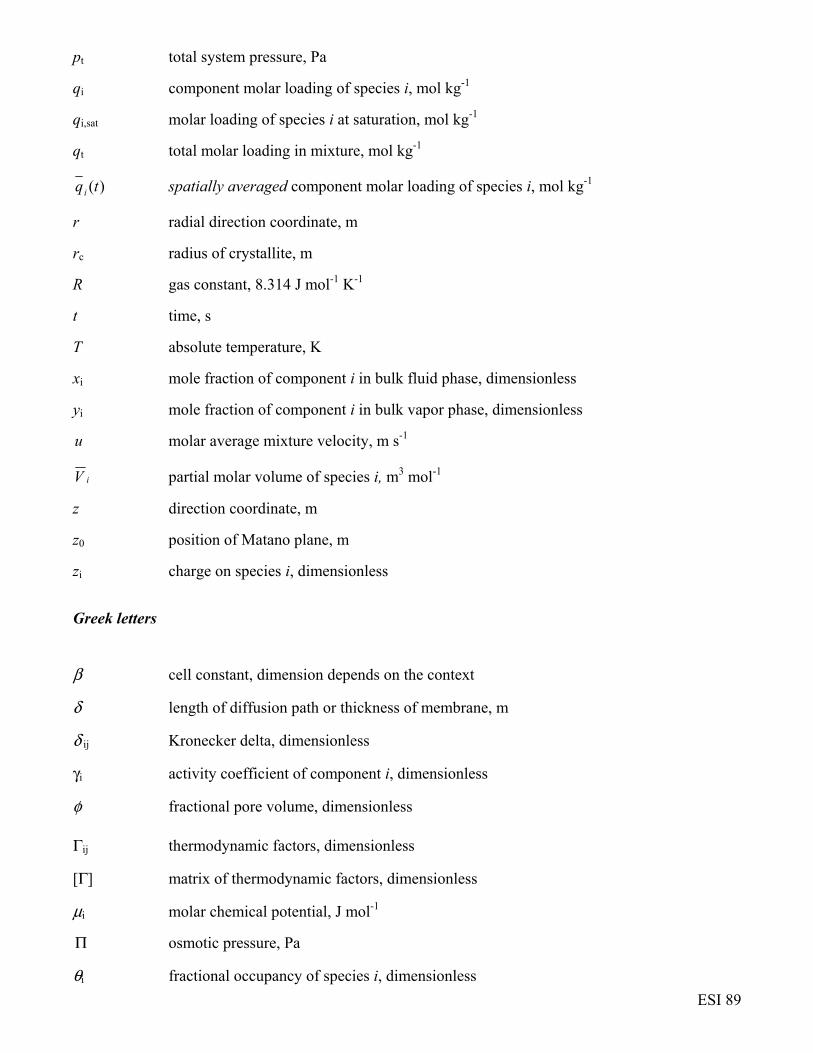
ESI 89

pt total system pressure, Pa

qi component molar loading of species i, mol kg-1

qi,sat molar loading of species i at saturation, mol kg-1

qt total molar loading in mixture, mol kg-1

)(tqi spatially averaged component molar loading of species i, mol kg-1

r radial direction coordinate, m

rc radius of crystallite, m

R gas constant, 8.314 J mol-1 K-1

t time, s

T absolute temperature, K

xi mole fraction of component i in bulk fluid phase, dimensionless

yi mole fraction of component i in bulk vapor phase, dimensionless

u molar average mixture velocity, m s-1

iV partial molar volume of species i, m3 mol-1

z direction coordinate, m

z0 position of Matano plane, m

zi charge on species i, dimensionless

Greek letters

β cell constant, dimension depends on the context

δ length of diffusion path or thickness of membrane, m

δ ij Kronecker delta, dimensionless

γi activity coefficient of component i, dimensionless

φ fractional pore volume, dimensionless

Γij thermodynamic factors, dimensionless

[Γ] matrix of thermodynamic factors, dimensionless

μi molar chemical potential, J mol-1

Π osmotic pressure, Pa

θi fractional occupancy of species i, dimensionless

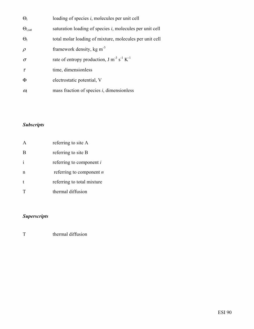
ESI 90

Θi loading of species i, molecules per unit cell

Θi,sat saturation loading of species i, molecules per unit cell

Θt total molar loading of mixture, molecules per unit cell

ρ framework density, kg m-3

σ rate of entropy production, J m-3 s-1 K-1

τ time, dimensionless

Φ electrostatic potential, V

ωi mass fraction of species i, dimensionless

Subscripts

A referring to site A

B referring to site B

i referring to component i

n referring to component n

t referring to total mixture

T thermal diffusion

Superscripts

T thermal diffusion

ESI 91

Table 1. NRTL parameters for acetone(1)/benzene(2)/carbon-tetrachloride(3) at 298 K. These

parameters are from Example 3.3.1 of Taylor and Krishna.11

ijτ jiτ jiij αα =

dimensionless dimensionless dimensionless

acetone(1)/benzene(2) -0.4605 0.76432 0.2

acetone(1)/carbon-tetrachloride(3)

-0.4279 1.5931 0.2

benzene(2)/carbon-tetrachloride(3)

-0.51821 0.7338 0.2

Table 2. NRTL parameters for acetone(1)/benzene(2)/methanol(3) at 298 K. The parameters have been

retrieved from the web.

ijτ jiτ jiij αα =

dimensionless dimensionless dimensionless

acetone(1)/benzene(2) 0.9247 -0.3826 0.3

acetone(1)/methanol(3) 0.3418 0.3827 0.3

benzene(2)/methanol(3) 0.5701 1.283 0.4

ESI 92

Table 3. Experimentally determined values of the Fick diffusivity matrix, expressed in units of 10-14 m2

s-1, as a function of the atom fractions of Cu, x1, and Ag, x2. These data at T = 998 K are from Table 8 of

Ziebold.33

x1 x2 D11 D12 D21 D22

0.021 0.869 1.2 0.07 -0.6 0.42

0.059 0.845 1.7 0.04 0.19 1.4

0.138 0.781 0.74 -0.28 0.81 1.6

0.036 0.727 2.3 0.7 0 0.63

0.112 0.719 2.1 0.5 0.21 1.3

0.073 0.593 1.2 0.28 0.83 0.76

0.075 0.586 1 0.22 0.96 0.91

0.14 0.457 1.9 1.1 2.1 2.4

0.131 0.34 0.99 0.09 1.7 1.3

0.351 0.18 2.5 1.6 2.8 4

0.351 0.042 3 1.7 0.57 2.8

0.418 0.03 3.1 0.75 0.29 2

0.446 0.025 3.2 0.73 0.81 3.3

0.585 0.048 2.3 0.53 0.81 3

0.603 0.129 2.3 1.11 1.8 3.1

0.629 0.095 2.4 1.04 1.9 3.6

0.666 0.027 1.8 0.2 0.18 1.5

0.663 0.007 2.1 2.4 0.04 1.8

0.798 0.059 1.11 0.28 0.42 1.5

0.81 0.039 0.93 0.2 0.17 1.4

0.816 0.024 0.73 -0.01 0.11 1.3

0.886 0.03 0.61 -0.03 0.08 0.93

0.901 0.021 0.43 -0.21 0.04 0.85

ESI 93

Table 4. NRTL parameters for methanol(1)-hexane(2) at various temperatures. The parameters are from

Clark and Rowley.40

TCBAT

Aijijij

ijij +== ;τ

2.0== jiij αα

12 21

ijB 1606.53 1540.7

ijC -4.2156 -3.7096

Table 5. NRTL parameters for glyercol(1)/acetone(2)/water(3) at 298 K. These parameters are from

Krishna et al.13

ijτ jiτ jiij αα =

dimensionless dimensionless dimensionless

glycerol(1)/acetone(2) 0.868 2.467 0.2

glycerol(1)/water(3) -1.29 -1.52 0.2

acetone(2)/water(3) -0.665 2.095 0.2

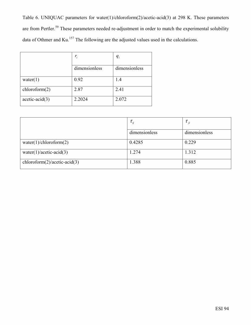
ESI 94

Table 6. UNIQUAC parameters for water(1)/chloroform(2)/acetic-acid(3) at 298 K. These parameters

are from Pertler.59 These parameters needed re-adjustment in order to match the experimental solubility

data of Othmer and Ku.157 The following are the adjusted values used in the calculations.

ir iq

dimensionless dimensionless

water(1) 0.92 1.4

chloroform(2) 2.87 2.41

acetic-acid(3) 2.2024 2.072

ijτ jiτ

dimensionless dimensionless

water(1)/chloroform(2) 0.4285 0.229

water(1)/acetic-acid(3) 1.274 1.312

chloroform(2)/acetic-acid(3) 1.388 0.885

ESI 95

Table 7. UNIQUAC parameters for water(1)/acetone(2)/ethyl-acetate(3) at 298 K. These parameters are

from Pertler.59

ir iq

dimensionless dimensionless

water(1) 0.92 1.4

acetone(2) 2.5735 2.336

ethyl-acetate(3) 3.4786 3.116

ijτ jiτ

dimensionless dimensionless

water(1)/acetone(2) 1.328 0.488

water(1)/ ethyl-acetate(3) 0.7705 0.2538

acetone(2)/ethyl-acetate(3) 1.3068 0.827

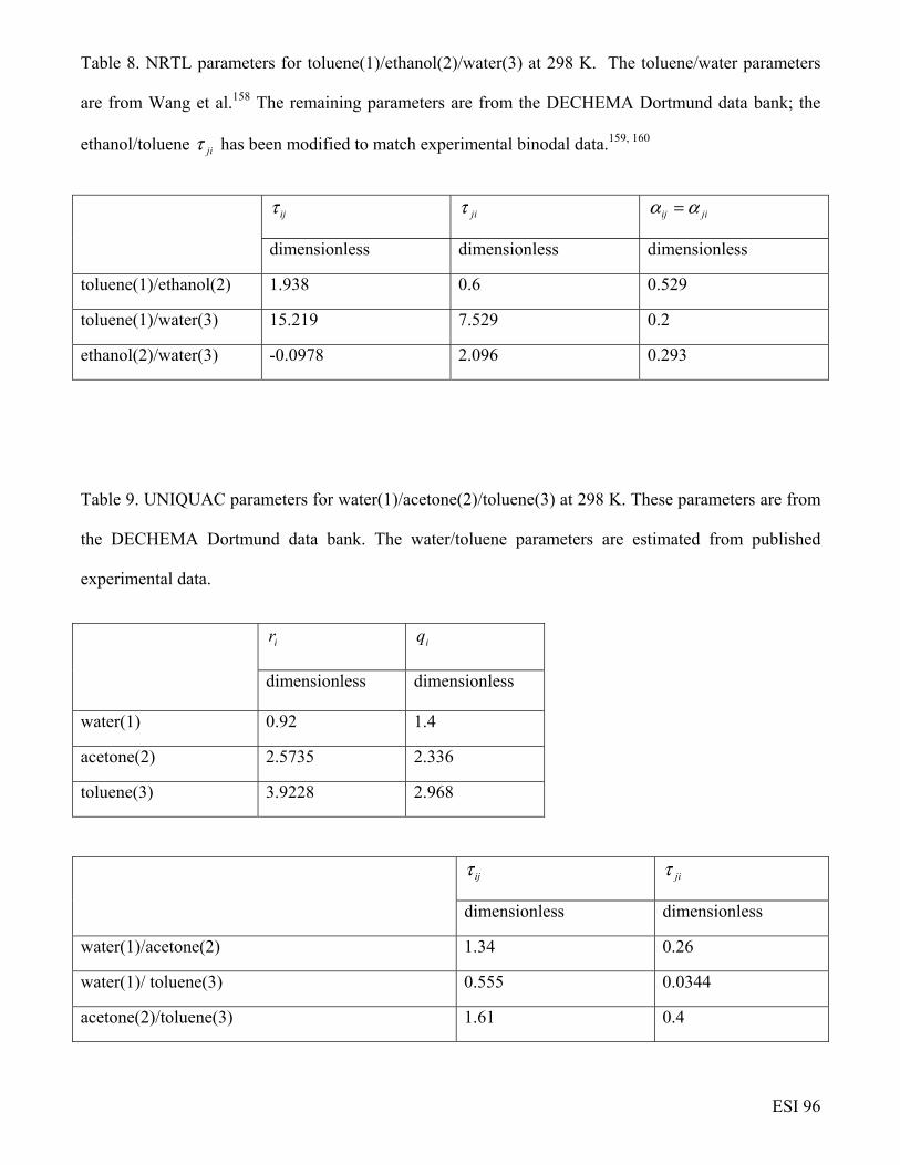
ESI 96

Table 8. NRTL parameters for toluene(1)/ethanol(2)/water(3) at 298 K. The toluene/water parameters

are from Wang et al.158 The remaining parameters are from the DECHEMA Dortmund data bank; the

ethanol/toluene jiτ has been modified to match experimental binodal data.159, 160

ijτ jiτ jiij αα =

dimensionless dimensionless dimensionless

toluene(1)/ethanol(2) 1.938 0.6 0.529

toluene(1)/water(3) 15.219 7.529 0.2

ethanol(2)/water(3) -0.0978 2.096 0.293

Table 9. UNIQUAC parameters for water(1)/acetone(2)/toluene(3) at 298 K. These parameters are from

the DECHEMA Dortmund data bank. The water/toluene parameters are estimated from published

experimental data.

ir iq

dimensionless dimensionless

water(1) 0.92 1.4

acetone(2) 2.5735 2.336

toluene(3) 3.9228 2.968

ijτ jiτ

dimensionless dimensionless

water(1)/acetone(2) 1.34 0.26

water(1)/ toluene(3) 0.555 0.0344

acetone(2)/toluene(3) 1.61 0.4

ESI 97

Table 10. UNIQUAC parameters for water(1)/caprolactam(2)/toluene(3). at 298.15 K. These parameters

are from Table 1, Chapter 7 of the PhD dissertation of Bollen.70

ir iq

dimensionless dimensionless

water(1) 0.92 1.4

caprolactam(2) 4.6106 3.724

toluene(3) 3.9928 2.968

ijτ jiτ

dimensionless dimensionless

water(1)/caprolactam(2) 0.1027043 3.647516849

water(1)/ toluene(3) 0.2563201 0.0964476

caprolactam(2)/toluene(3) 0.3324973 1.4351863

ESI 98

Table 11. UNIQUAC parameters for water(1)/caprolactam(2)/benzene(3) at 298.15 K. These parameters

are from Table 1, Chapter 7 of the PhD dissertation of Bollen.70

ir iq

dimensionless dimensionless

water(1) 0.92 1.4

caprolactam(2) 4.6106 3.724

benzene(3) 3.1878 2.4

ijτ jiτ

dimensionless dimensionless

water(1)/caprolactam(2) 1.5339381 1.7321924

water(1)/ benzene(3) 0.3259823 0.1101953

caprolactam(2)/benzene(3) 1.4594085 0.8758174

ESI 99

Table 12. UNIQUAC parameters for toluene(1)/water(2)/propionic-acid(2)/water(3) at 298.15 K. These

parameters are from Table 6 of Kim and Park.161 However, there is some uncertainty about the units of

the energy parameters listed in Table 6 because the units are not specified. Furthermore, equation (16)

of Kim and Park161 appears to contain a typo. Due to the combination of the uncertainties, our binodal

curve do not correspond with the experimental data. Therefore, the calculations presented here must be

viewed as being consistent for a partially miscible (hypothetical) mixture for which the following set of

UNIQUAC parameters are valid.

ir iq

dimensionless dimensionless

toluene(1) 3.9928 2.968

Propionic-acid(2) 2.9 2.58

water(3) 0.92 1.4

ijτ jiτ

dimensionless dimensionless

toluene(1) / propionic-acid (2) 1.08985977 0.86688385

toluene(1)/ water(3) 0.81980947 0.3296506

Propionic-acid (2)/ water(3) 1.21111669 0.61226107

ESI 100

Table 13. UNIQUAC parameters for ethylacetate(1)/propionic-acid(2)/water(3) at 298.15 K. These

parameters are from Table 6 of Kim and Park.161 However, there is some uncertainty about the units of

the energy parameters listed in Table 6 because the units are not specified. Furthermore, equation (16)

of Kim and Park161 appears to contain a typo. Due to the combination of the uncertainties, our binodal

curve do not correspond with the experimental data. Therefore, the calculations presented here must be

viewed as being consistent for a partially miscible (hypothetical) mixture for which the following set of

UNIQUAC parameters are valid.

ir iq

dimensionless dimensionless

ethylacetate(1) 3.4786 3.116

Propionic-acid(2) 2.9 2.58

water(3) 0.92 1.4

ijτ jiτ

dimensionless dimensionless

ethylacetate (1)/ propionic-acid (2) 0.94875404 2.69011546

ethylacetate (1)/ water(3) 0.19953302 0.33562196

Propionic-acid (2)/ water(3) 3.28217216 1.9470615

ESI 101

Table 14. 1-site Langmuir-Freundlich parameters for ethene, ethane, propene and propane in ZIF-8.

The T-dependent parameters are obtained by fitting the combined sets of pure component isotherm data

of Li et al.140 and Böhme et al.162 determined for a variety of temperatures in the range 273 K to 408 K.

ν

ν

bp

bpqq sat +

=1

=

RT

EbbA exp0

qsat

mol kg-1

b0

ν−Pa

E

kJ mol-1

ν

dimensionless

ethene 12

9.37×10-11 21.5 1.08

ethane 12

8.55×10-11 23.2 1.08

propene 5.2

4.57×10-11 33.9 1

propane 5.2

1.39×10-10 31.3 1

ESI 102

24. References

(1) Onsager, L. Theories and Problems of Liquid Diffusion, Annals N.Y. Acad. Sci. 1945, 46, 241-265. (2) de Groot, S. R.; Mazur, P. Non-Equilibrium Thermodynamics; North-Holland Publishing Co.: Amsterdam, 1962. (3) Truesdell, C. A. Rational Thermodynamics; McGraw-Hill: New York, 1969. (4) Maxwell, J. C. On the dynamical theory of gases, Phil. Trans. Roy. Soc. 1866, 157, 49-88. (5) Stefan, J. Über das Gleichgewicht und die Bewegung insbesondere die Diffusion von Gasgemengen, Sitzber. Akad. Wiss. Wien. 1871, 63, 63-124. (6) Hirschfelder, J. O.; Curtiss, C. F.; Bird, R. B. Molecular theory of gases and liquids; Second Corrected Printing, John Wiley: New York, USA, 1964. (7) Toor, H. L. Diffusion in Three-Component Gas Mixtures, A.I.Ch.E.J. 1957, 3, 198-207. (8) Toor, H. L. Solution of the Linearised Equations of Multi-component Mass Transfer, A.I.Ch.E.J. 1964, 10, 448-465. (9) Stewart, W. E.; Prober, R. Matrix Calculation of Multi-component Mass Transfer in Isothermal Systems, Ind. Eng. Chem., Fundam. 1964, 3, 224-235. (10) Krishna, R.; Standart, G. L. A multicomponent film model incorporating a general matrix method of solution to the Maxwell-Stefan equations, A.I.Ch.E.J. 1976, 22, 383-389. (11) Taylor, R.; Krishna, R. Multicomponent mass transfer; John Wiley: New York, 1993. (12) Standart, G. L.; Taylor, R.; Krishna, R. The Maxwell-Stefan formulation of irreversible thermodynamics for simultaneous heat and mass transfer, Chem. Eng. Commun. 1979, 3, 277-289. (13) Krishna, R.; Low, C. Y.; Newsham, D. M. T.; Olivera Fuentes, C. G.; Paybarah, A. Liquid Liquid Equilibrium in the System Glycerol Water Acetone at 25 oC, Fluid Phase Equilib. 1989, 45, 115-120. (14) Krishna, R.; van Baten, J. M. The Darken relation for multicomponent diffusion in liquid mixtures of linear alkanes. An investigation using Molecular Dynamics (MD) simulations, Ind. Eng. Chem. Res. 2005, 44, 6939-6947. (15) Fuller, E. N.; Schettler, P. D.; Giddings, J. C. A new method for prediction of binary gas-phase diffusion coefficients, Ind. Eng. Chem. 1966, 58, 19-27. (16) Darken, L. S. Diffusion, Mobility and Their Interrelation through Free Energy in Binary Metallic Systems, Trans. AIME 1948, 175, 184-201. (17) Darken, L. S. Diffusion of Carbon in Austenite with a Discontinuity in Composition, Trans. AIME 1949, 180, 430-438. (18) Shieh, J. C.; Lyons, P. A. Transport Properties of Liquid n-Alkanes, J. Phys. Chem. 1969, 73, 3258-3264. (19) Bidlack, D. L.; Anderson, D. K. Mutual diffusion in the system hexane-hexadecane, J. Phys. Chem. 1964, 68, 206-208. (20) Helbaek, M.; Hafskjold, B.; Dysthe, D. K.; Sorland, G. H. Self-diffusion coefficients of methane or ethane mixtures with hydrocarbons at high pressure by NMR, J. Chem. Eng. Data 1996, 41, 598-603. (21) Krishna, R.; van Baten, J. M. Unified Maxwell-Stefan description of binary mixture diffusion in micro- and meso- porous materials, Chem. Eng. Sci. 2009, 64, 3159-3178. (22) Liu, X.; Bardow, A.; Vlugt, T. J. H. Multicomponent Maxwell-Stefan Diffusivities at Infinite Dilution, Ind. Eng. Chem. Res. 2011, 50, 4776-4782.

ESI 103

(23) Krishna, R.; van Baten, J. M. MD simulations of diffusivities in methanol – n-hexane mixtures near the liquid-liquid phase splitting region, Chem Eng Technol 2006, 29, 516-519. (24) Krishna, R.; van Baten, J. M. Validating the Darken relation for diffusivities in fluid mixtures of varying densities by use of MD simulations, Chem Eng Technol 2006, 29, 761-765. (25) Wesselingh, J. A.; Krishna, R. Mass transfer in multicomponent mixtures; Delft University Press: Delft, 2000. (26) Hsu, Y.-D.; Chen, Y.-P. Correlation of the mutual diffusion coefficients of binary liquid mixtures, Fluid Phase Equilibr. 1998, 152, 149-168. (27) Krishna, R.; Standart, G. L. Mass and energy transfer in multicomponent systems, Chem. Eng. Commun. 1979, 3, 201-275. (28) Krishna, R. A Unified Theory of Separation Processes Based on Irreversible Thermodynamics, Chem. Eng. Commun. 1987, 59, 33-64. (29) Krishna, R.; van Baten, J. M. Onsager coefficients for binary mixture diffusion in nanopores, Chem. Eng. Sci. 2008, 63, 3120-3140. (30) Cullinan, H. T.; Toor, H. L. Diffusion in the Three-Component Liquid System: Acetone-Benzene Carbon Tetrachloride, J. Phys. Chem. 1965, 69, 3941-3949. (31) Rehfeldt, S.; Stichlmair, J. Measurement and prediction of multicomponent diffusion coefficients in four ternary liquid systems, Fluid Phase Equilib. 2010, 290, 1-14. (32) Rehfeldt, S. Mehrkomponentendiffusion in Flüssigkeiten, Technische Universität München, München, 2009. (33) Ziebold, T. O. Ternary Diffusion in Copper-Silver-Gold Alloys, Massachusetts Institute of Technology, Cambridge, Massachusetts, 1965. (34) Duncan, J. B.; Toor, H. L. An Experimental Study of Three Component Gas Diffusion, A.I.Ch.E.J. 1962, 8, 38-41. (35) Arnold, K. R.; Toor, H. L. Unsteady Diffusion in Ternary Gas Mixtures, A.I.Ch.E.J. 1967, 13, 909-914. (36) Bres, M.; Hatzfeld, C. Three-Gas Diffusion - Experimental and Theoretical Study, Pflügers Arch. 1977, 371, 227-233. (37) Boudin, L.; Götz, D.; Grec, B. Diffusion Models of Multicomponent Mixtures in the Lung, ESAIM: Proceedings, 90-103, 2010. http://dx.doi.org/10.1051/proc/2010008. (38) Chevrolet, J.-C. Helium oxygen mixtures in the intensive care unit, Critical Care 2001, 5, 179–181. (39) Fullarton, D.; Schlünder, E. U. Diffusion Distillation - A New Separation .Process for Azeotropic Mixtures - Part I: Selectivity and Transfer Efficiency, Chem. Eng. Process. 1986, 20, 255-263. (40) Clark, W. M.; Rowley, R. L. The mutual diffusion coefficient of methanol - n-hexane near the consolute point, A.I.Ch.E.J. 1986, 32, 1125-1131. (41) Haase, R.; Siry, M. Diffusion im kritischen entmischungsgebiet binärer flüssiger systeme, Z. Phys. Chem. 1968, 57, 56-73. (42) Vitagliano, V.; Sartorio, R.; Chiaravalle, E.; Ortona, O. Diffusion and Viscosity in Water-Triethylamine Mixtures at 19 and 20 “C, J. Chem. Eng. Data 1980, 25, 121-124. (43) Myerson, A. S.; Senol, D. Diffusion Coefficients near the Spinodal Curve, A.I.Ch.E.J. 1984, 30, 1004-1006. (44) Chang, Y. C.; Myerson, A. S. Diffusivity of Glycine in Concentrated Solutions and Supersaturated Aqueous Solutions, A.I.Ch.E.J. 1986, 32, 1567-1569. (45) Cussler, E. L. Diffusion: Mass Transfer in Fluid Systems; 3rd Edition, Cambridge University Press: Cambridge, 2007. (46) Garside, J. Industrial Crystallization from Solution, Chem. Eng. Sci. 1985, 40, 3-26. (47) Louhi-Kultanen, M.; Kallas, J.; Partanen, J.; Sha, Z.; Oinas, P.; Palosaari, S. The influence of multicomponent diffusion on crystal growth in electrolyte soluti �ons , Chem. Eng. Sci. 2001, 56, 3505-3515.

ESI 104

(48) Matos Lopes, M. L. S.; Nieto de Castro, C. A.; Sengers, J. V. Mutual Diffusivity of a Mixture of n-Hexane and Nitrobenzene Near Its Consolute Point, Int. J. Thermophys. 1992, 13, 283-294. (49) Wu, G.; Fiebig, M.; Leipertz Messung des bin iren Diffusionskoeffizienten in einem Entmischungssystem mit Hilfe der Photonen-Korrelationsspektroskopie, Wärme- und Stoffübertragung 1988, 22, 365-371. (50) Glicksman, M. E. Diffusion in Solids: Field Theory, Solid-state Principles, and Applications; John Wiley: New York, 2000. (51) Cahn, J. W.; Hilliard, J. E. Free Energy of a Nonuniform System. II. Nucleation in a Two-Component Incompressible Fluid, J. Chem. Phys. 1959, 31, 688-699. (52) Cahn, J. W. On Spinodal Decomposition, J. Chem. Phys. 1961, 9, 795-801. (53) Grossmann, T.; Winkelmann, J. Ternary Diffusion Coefficients of Glycerol + Acetone + Water by Taylor Dispersion Measurements at 298.15 K, J. Chem. Eng. Data 2005, 50, 1396-1403. (54) Grossmann, T.; Winkelmann, J. Ternary Diffusion Coefficients of Glycerol + Acetone + Water by Taylor Dispersion Measurements at 298.15 K. 2. Acetone-Rich Region, J. Chem. Eng. Data 2007, 52, 336-340. (55) Grossmann, T.; Winkelmann, J. Ternary Diffusion Coefficients of Glycerol + Acetone + Water by Taylor Dispersion Measurements at 298.15 K. 3. Water-Rich Region, J. Chem. Eng. Data 2007, 52, 341-344. (56) Vitagliano, V.; Sartorio, R.; Scala, S.; Spaduzzi, D. Diffusion in a Ternary System and the Critical Mixing Point, J. Solution Chem. 1978, 7, 605-621. (57) Buzatu, D.; Buzatu, F. D.; Paduano, L.; Sartorio, R. Diffusion Coefficients for the Ternary System Water + Chloroform + Acetic Acid at 25 °C, J. Solution Chem. 2007, 36, 1373-1384. (58) Clark, W. M.; Rowley, R. L. Ternary Liquid Diffusion Coefficients Near Plait Points, Int. J. Thermophys. 1986, 6, 631-642. (59) Pertler, M. Die Mehrkomponenten-Diffuson in nicht vollständig mischbaren Flüssigkeiten, Technische Universität München, München, 1996. (60) Krishna, R.; Low, C. Y.; Newsham, D. M. T.; Olivera-Fuentes, C. G.; Standart, G. L. Ternary mass transfer in liquid-liquid extraction, Chem. Eng. Sci. 1985, 40, 893-903. (61) Haeberl, M.; Blass, E. Multicomponent Effects in Liquid-Liquid Extraction, Chem. Eng. Res. Des., Trans. IChemE. 1999, 77, 647-655. (62) Jackson, R. Diffusion in Ternary Mixtures with and without Phase Boundaries, Ind. Eng. Chem., Fundam. 1977, 16, 304-306. (63) Ruschak, K. J.; Miller, C. A. Spontaneous Emulsification in Ternary Systems with Muss Transfer, Ind. Eng. Chem., Fundam. 1972, 11, 534-540. (64) Miller, C. A. Spontaneous Emulsification Produced by Diffusion - A Review, Colloids Surf. 1988, 29, 89-102. (65) Sitnikova, N. L.; Sprik, R.; Wegdam, G.; Eiser, E. Spontaneously Formed trans-Anethol/Water/Alcohol Emulsions: Mechanism of Formation and Stability, Langmuir 2005, 21, 7083-7089. (66) Lecuyer, C. Water on Earth; John Wiley & Sons, Inc.: Hoboken, USA., 2013. (67) Vitale, S. A.; Katz, J. L. Liquid Droplet Dispersions Formed by Homogeneous Liquid-Liquid Nucleation: “The Ouzo Effect”, Langmuir 2003, 19, 4105-4110. (68) Ganachaud, F.; Katz, J. L. Nanoparticles and Nanocapsules Created Using the Ouzo Effect: Spontaneous Emulsification as an Alternative to Ultrasonic and High-Shear Devices ChemPhysChem 2005, 6, 209-216. (69) Ullmann, A.; Gat, S.; Ludmer, Z.; Brauner, N. Phase Separation of Partially Miscible Solvent Systems: Flow Phenomena and Heat and Mass Transfer Applications, Rev. Chem. Eng. 2008, 24, 159-262. (70) Bollen, A. M. Collected tales on mass transfer in liquids, Ph.D. Dissertation, Rijksuniversiteit Groningen, Groningen, 1999. http://dissertations.ub.rug.nl/faculties/science/1999/a.m.bollen/

ESI 105

(71) van den Berg, G. B.; Smolders, C. A. Diffusional phenomena in membrane separation processes, J. Membr. Sci. 1992, 73, 103-118. (72) Reuvers, A. J.; Smolders, C. A. Formation of membranes by means of immersion precipitation Part II. The mechanism of formation of membranes prepared from the system cellulose acetate - acetone - water, J. Membr. Sci. 1987, 34, 67-86. (73) Prakash, S. S.; Francis, L. F.; Scriven, L. E. Microstructure evolution in dry cast cellulose acetate membranes by cryo-SEM, J. Membr. Sci. 2006, 283, 328-338. (74) Shojaie, S.; Krantz, W. B.; Greenberg, A. R. Dense polymer film and membrane formation via the dry-cast process Part I. Model development, J. Membr. Sci. 1994, 94, 255-280. (75) Shojaie, S.; Krantz, W. B.; Greenberg, A. R. Dense polymer film and membrane formation via the dry-cast process Part II. Model validation and morphological studies, J. Membr. Sci. 1994, 94, 281-298. (76) Coumans, W. J.; Kerkhof, P. J. A. M.; Bruin, S. Theoretical and Practical Aspects of Aroma Retention in Spray Drying and Freeze Drying, Dry. Technol. 1994, 12, 99-149. (77) Gupta, P. K.; Cooper, A. R. The [D] Matrix for Multicomponent Diffusion, Physica 1971, 54, 39-59. (78) Kirkaldy, J. S. Diffusion in Multicomponent Metallic Systems, Canad. J. Phys. 1957, 35, 435-4440. (79) Varshneya, A. K.; Cooper, A. R. Diffusion in the System K2O-SrO-SiO2: III, Interdiffusion Coefficients, J. Am. Ceram.. Soc. 1972, 55, 312-317. (80) Vielzeuf, D.; Saúl, A. Uphill diffusion, zero-flux planes and transient chemical solitary waves in garnet, Contrib. Mineral. Petrol. 2011, 161, 683-702. (81) Christensen, N. H. Multiphase Ternary Diffusion Couples, J. Am. Ceram.. Soc. 1977, 60, 293-296. (82) Taylor, R.; Krishna, R.; Kooijman, H. Real-World Modeling of Distillation, Chem. Eng. Prog. 2003, 99 (7), 28-39. (83) Krishna, R.; Martinez, H. F.; Sreedhar, R.; Standart, G. L. Murphree point efficiencies in multicomponent systems, Trans. Inst. Chem. Eng. 1977, 55, 178-183. (84) Springer, P. A. M.; Baur, R.; Krishna, R. Influence of interphase mass transfer on the composition trajectories and crossing of boundaries in ternary azeotropic distillation, Sep. Purif. Technol. 2002, 29, 1-13. (85) Springer, P. A. M.; Baur, R.; Krishna, R. Composition trajectories for heterogeneous azeotropic distillation in a bubble-cap tray column: Influence of mass transfer, Chem. Eng. Res. Des. 2003, 81, 413-426. (86) Springer, P. A. M.; Buttinger, B.; Baur, R.; Krishna, R. Crossing of the distillation boundary in homogeneous azeotropic distillation: Influence of interphase mass transfer, Ind. Eng. Chem. Res. 2002, 41, 1621-1631. (87) Springer, P. A. M.; Krishna, R. Crossing of boundaries in ternary azeotropic distillation: Influence of interphase mass transfer, Int. Commun. Heat Mass Transf. 2001, 28, 347-356. (88) Springer, P. A. M.; van der Molen, S.; Baur, R.; Krishna, R. Experimental verification of the necessity to use the Maxwell-Stefan formulation in describing trajectories during azeotropic distillation, Chem. Eng. Res. Des. 2002, 80, 654-666. (89) Springer, P. A. M.; van der Molen, S.; Krishna, R. The need for using rigorous rate-based models for simulations of ternary azeotropic distillation, Comput. Chem. Eng. 2002, 26, 1265-1279. (90) Baur, R.; Taylor, R.; Krishna, R.; Copati, J. A. Influence of mass transfer in distillation of mixtures with a distillation boundary, Chem. Eng. Res. Des. 1999, 77, 561-565. (91) Doherty, M. F.; Malone, M. F. Conceptual Design of Distillation Systems; McGraw-Hill: New York, 2001. (92) Higler, A.; Chande, R.; Taylor, R.; Baur, R.; Krishna, R. Nonequilibrium Modelling of Three-Phase distillation, Comput. Chem. Eng. 2004, 28, 2021-2036. (93) Vinograd, J. R.; McBain, J. W. Diffusion of Electrolytes and Ions in their Mixtures, J. Am. Chem. Soc. 1941, 63, 2008-2015.

ESI 106

(94) Kraaijeveld, G.; Wesselingh, J. A. The Kinetics of Film-Diffusion-Limited Ion Exchange, Chem. Eng. Sci. 1993, 48, 467-473. (95) Yang, Y.; Pintauro, P. N. Multicomponent Space-Charge Transport Model for Ion-Exchange Membranes, A.I.Ch.E.J. 2000, 46, 1177-1190. (96) Platten, J. K. The Soret Effect: A Review of Recent Experimental Results, J. Appl. Mech. 2006, 73, 5-15. (97) Huang, F.; Chakraborty, P.; Lundstrom, C. C.; Holmden, C.; Glessner, J. J. G.; Kieffer, S. W.; Lesher, C. E. Isotope fractionation in silicate melts by thermal diffusion, Nature 2010, 464, 396-401. (98) McDougall, T. J. Double-diffusive convection caused by coupled molecular diffusion, J. Fluid Mech. 1963, 126, 379-397. (99) Kärger, J.; Ruthven, D. M.; Theodorou, D. N. Diffusion in Nanoporous Materials; Wiley - VCH: Weinheim, 2012. (100) Krishna, R.; van Baten, J. M. In Silico Screening of Zeolite Membranes for CO2 Capture, J. Membr. Sci. 2010, 360, 323-333. (101) Krishna, R.; van Baten, J. M. In silico screening of metal-organic frameworks in separation applications, Phys. Chem. Chem. Phys. 2011, 13, 10593-10616. (102) Thomas, A. Functional Materials: From Hard to Soft Porous Frameworks, Angew. Chem. Int. Ed. 2010, 49, 8328 – 8344. (103) Krishna, R. Diffusion in Porous Crystalline Materials, Chem. Soc. Rev. 2012, 41, 3099-3118. (104) Krishna, R. The Maxwell-Stefan Description of Mixture Diffusion in Nanoporous Crystalline Materials, Microporous Mesoporous Mater. 2014, 185, 30-50. (105) Krishna, R. Describing the diffusion of guest molecules inside porous structures, J. Phys. Chem. C 2009, 113, 19756-19781. (106) Ruthven, D. M.; Farooq, S.; Knaebel, K. S. Pressure swing adsorption; VCH Publishers: New York, 1994. (107) Krishna, R.; Baur, R. Modelling issues in zeolite based separation processes, Sep. Purif. Technol. 2003, 33, 213-254. (108) He, Y.; Krishna, R.; Chen, B. Metal-Organic Frameworks with Potential for Energy-Efficient Adsorptive Separation of Light Hydrocarbons, Energy Environ. Sci. 2012, 5, 9107-9120. (109) Farooq, S.; Rathor, M. N.; Hidajat, K. A Predictive Model for a Kinetically Controlled Pressure Swing Adsorption Separation Process, Chem. Eng. Sci. 1993, 48, 4129-4141. (110) Farooq, S. Sorption and Diffusion of Oxygen and Nitrogen in Molecular- Sieve RS-10, Gas Sep. Purif. 1995, 9, 205-212. (111) Krishna, R.; van Baten, J. M. Investigating the Influence of Diffusional Coupling on Mixture Permeation across Porous Membranes J. Membr. Sci. 2013, 430, 113-128. (112) Caro, J.; Noack, M. Zeolite membranes - Recent Developments and Progress, Microporous Mesoporous Mat. 2008, 115, 215-233. (113) Ruthven, D. M. Principles of Adsorption and Adsorption Processes; John Wiley: New York, 1984. (114) Skoulidas, A. I.; Sholl, D. S.; Krishna, R. Correlation effects in diffusion of CH4/CF4 mixtures in MFI zeolite. A study linking MD simulations with the Maxwell-Stefan formulation, Langmuir 2003, 19, 7977-7988. (115) Chempath, S.; Krishna, R.; Snurr, R. Q. Nonequilibrium MD simulations of difusion of binary mixtures containing short n-alkanes in faujasite, J. Phys. Chem. B 2004, 108, 13481-13491. (116) Hansen, N.; Keil, F. J. Multiscale modeling of reaction and diffusion in zeolites: from the molecular level to the reactor, Soft Mater. 2012, 10, 179-201. (117) Krishna, R.; van Baten, J. M. Hydrogen Bonding Effects in Adsorption of Water-alcohol Mixtures in Zeolites and the Consequences for the Characteristics of the Maxwell-Stefan Diffusivities, Langmuir 2010, 26, 10854-10867.

ESI 107

(118) Krishna, R.; van Baten, J. M. Influence of Adsorption Thermodynamics on Guest Diffusivities in Nanoporous Crystalline Materials, Phys. Chem. Chem. Phys. 2013, 15, 7994-8016. (119) Krishna, R.; van Baten, J. M. An investigation of the characteristics of Maxwell-Stefan diffusivities of binary mixtures in silica nanopores, Chem. Eng. Sci. 2009, 64, 870-882. (120) Mason, E. A.; Malinauskas, A. P. Gas Transport in Porous Media: The Dusty-Gas Model; Elsevier: Amsterdam, 1983. (121) Krishna, R.; van Baten, J. M. Investigating the validity of the Knudsen prescription for diffusivities in a mesoporous covalent organic framework, Ind. Eng. Chem. Res. 2011, 50, 7083-7087. (122) Krishna, R.; van Baten, J. M. Investigating the validity of the Bosanquet formula for estimation of diffusivities in mesopores, Chem. Eng. Sci. 2012, 69, 684-688. (123) Garg, D. R.; Ruthven, D. M. Effect of the concentration dependence of diffusivity on zeolitic sorption curves, Chem. Eng. Sci. 1972, 27, 417-423. (124) Niessen, W.; Karge, H. G. Diffusion of p-xylene in Single and Binary Systems Investigated by FTIR Spectroscopy, Microporous Mater. 1993, 1, 1-8. (125) Krishna, R.; van Baten, J. M. Investigating cluster formation in adsorption of CO2, CH4, and Ar in zeolites and metal organic frameworks at sub-critical temperatures, Langmuir 2010, 26, 3981-3992. (126) Krishna, R.; van Baten, J. M. Highlighting a variety of unusual characteristics of adsorption and diffusion in microporous materials induced by clustering of guest molecules, Langmuir 2010, 26, 8450-8463. (127) Krishna, R.; van Baten, J. M. Highlighting Pitfalls in the Maxwell-Stefan Modeling of Water-Alcohol Mixture Permeation across Pervaporation Membranes, J. Membr. Sci. 2010, 360, 476-482. (128) Krishna, R.; van Baten, J. M. A molecular dynamics investigation of the unusual concentration dependencies of Fick diffusivities in silica mesopores, Microporous Mesoporous Mater. 2011, 138, 228-234. (129) Krishna, R.; van Baten, J. M. A rationalization of the Type IV loading dependence in the Kärger-Pfeifer classification of self-diffusivities, Microporous Mesoporous Mater. 2011, 142, 745-748. (130) Chmelik, C.; Bux, H.; Caro, J.; Heinke, L.; Hibbe, F.; Titze, T.; Kärger, J. Mass transfer in a Nanoscale Material Enhanced by an Opposing Flux, Phys. Rev. Lett. 2010, 104, 085902. (131) Myers, A. L.; Prausnitz, J. M. Thermodynamics of Mixed Gas Adsorption, A.I.Ch.E.J. 1965, 11, 121-130. (132) Krishna, R.; van Baten, J. M. A molecular dynamics investigation of the diffusion characteristics of cavity-type zeolites with 8-ring windows, Microporous Mesoporous Mater. 2011, 137, 83-91. �(133) Bhadra, S. J.; Farooq, S. Separation of Methane Nitrogen Mixture by Pressure Swing Adsorption for Natural Gas Upgrading, Ind. Eng. Chem. Res. 2011, 50, 14030-14045. (134) Majumdar, B.; Bhadra, S. J.; Marathe, R. P.; Farooq, S. Adsorption and Diffusion of Methane and Nitrogen in Barium Exchanged ETS-4, Ind. Eng. Chem. Res. 2011, 50, 3021-3034. (135) Habgood, H. W. The Kinetics of Molecular Sieve Action. Sorption of Nitrogen-Methane Mixtures by Linde Molecular Sieve 4A, Canad. J. Chem. 1958, 36, 1384-1397. (136) Kuznicki, S. M.; Bell, V. A.; Nair, S.; Hillhouse, H. W.; Jacubinas, R. M.; Braunbarth, C. M.; Toby, B. H.; Tsapatsis, M. A titanosilicate molecular sieve with adjustable pores for size-selective adsorption of molecules, Nature 2001, 412, 720-724. (137) Yang, R. T. Adsorbents: Fundamentals and Applications; John Wiley & Sons, Inc.: Hoboken, New Jersey, 2003. (138) Chen, Y. D.; Yang, R. T.; Uawithya, P. Diffusion of oxygen, nitrogen and their mixtures in Carbon Molecular-Sieve, A.I.Ch.E.J. 1994, 40, 577-585. (139) Carlson, N. W.; Dranoff, J. S. Competitive adsorption of methane and ethane on 4A zeolite. Fundamentals of Adsorption; Edited by A.I. Liapis, AIChE: New York, 1986.

ESI 108

(140) Li, K.; Olson, D. H.; Seidel, J.; Emge, T. J.; Gong, H.; Zeng, H.; Li, J. Zeolitic Imidazolate Frameworks for Kinetic Separation of Propane and Propene, J. Am. Chem. Soc. 2009, 131, 10368-10369. (141) Khalighi, M.; Chen, Y. F.; Farooq, S.; Karimi, I. A.; Jiang, J. W. Propylene/Propane Separation Using SiCHA, Ind. Eng. Chem. Res. 2013, 52, 3877-3892. (142) Saint-Remi, J. C.; Baron, G. V.; Denayer, J. F. M. Non-Uniform Chain Length Dependent Diffusion of Short 1-Alcohols in SAPO-34 in Liquid Phase, J. Phys. Chem. C 2013, 117, 9758-9765. (143) Remy, T.; Saint-Remi, J. C.; Singh, R.; Webley, P. A.; Baron, G. V.; Denayer, J. F. M. Adsorption and Separation of C1-C8 Alcohols on SAPO-34, J. Phys. Chem. C 2011, 115, 8117-8125. (144) Krishna, R.; van Baten, J. M. Entropy-based Separation of Linear Chain Molecules by Exploiting Differences in the Saturation Capacities in Cage-type Zeolites, Sep. Purif. Technol. 2011, 76, 325-330. (145) Kärger, J.; Bülow, M. Theoretical Prediction of Uptake Behaviour in Adsorption Kinetics of Binary Gas Mixtures Using Irreversible Thermodynamics, Chem. Eng. Sci. 1975, 30, 893-896. (146) Krishna, R.; van Baten, J. M. Investigating the Relative Influences of Molecular Dimensions and Binding Energies on Diffusivities of Guest Species Inside Nanoporous Crystalline Materials J. Phys. Chem. C 2012, 116, 23556-23568. (147) Krishna, R. Multicomponent surface diffusion of adsorbed species - A description based on the generalized Maxwell-Stefan equations, Chem. Eng. Sci. 1990, 45, 1779-1791. (148) Karge, H. G. Infrared Spectroscopic Investigation of Diffusion, Co-diffusion and Counter-diffusion of Hydrocarbon Molecules in Zeolites, C.R. Chim. 2005, 8, 303-319. (149) Titze, T.; Chmelik, C.; Kärger, J.; van Baten, J. M.; Krishna, R. Uncommon Synergy Between Adsorption and Diffusion of Hexane Isomer Mixtures in MFI Zeolite Induced by Configurational Entropy Effects J. Phys. Chem. C 2014, 118, 2660-2665. (150) Fernandez, M.; Kärger, J.; Freude, D.; Pampel, A.; van Baten, J. M.; Krishna, R. Mixture Diffusion in Zeolites Studied by MAS PFG NMR and Molecular Simulation, Microporous Mesoporous Mater. 2007, 105, 124-131. (151) Pan, Y.; Li, T.; Lestari, G.; Lai, Z. Effective Separation of Propylene/Propane Binary Mixtures by ZIF-8 Membranes, J. Membr. Sci. 2012, 390-391, 93-98. (152) Geus, E. R.; van Bekkum, H.; Bakker, W. J. W.; Moulijn, J. A. High-temperature Stainless Steel Supported Zeolite (MFI) Membranes: Preparation, Module Construction, and Permeation Experiments, Microporous Mater. 1993, 1, 131-147. (153) Bakker, W. J. W. Structured systems in gas separation, Ph.D. Dissertation, Delft University of Technology, Delft, 1999. (154) Matsufuji, T.; Watanabe, K.; Nishiyama, N.; Egashira, Y.; Matsukata, M.; Ueyama, K. Permeation of Hexane Isomers Through an MFI Membrane, Ind. Eng. Chem. Res. 2000, 39, 2434-2438. (155) Matsufuji, T.; Nishiyama, N.; Matsukata, M.; Ueyama, K. Separation of Butane and Xylene Isomers with MFI-type Zeolitic Membrane Synthesized by a Vapor-Phase Transport Method, J. Membr. Sci. 2000, 178, 25-34. (156) Kolvenbach, R.; Al-Yassir, N.; S.S. Al-Khattaf, S. S.; Gobin, O. C.; Ahn, J. H.; Jentys, A.; Lercher, J. A. A comparative study of diffusion of benzene/p-xylene mixtures in MFI particles, pellets and grown membranes, Catal. Today 2011, 168, 147-157. (157) Othmer, D. F.; Ku, P. L. Solubility Data for Ternary Liquid Systems. Acetic Acid and Formic Acid Distributed between Chloroform and Water, J. Chem. Eng. Data 1960, 5, 42-44. (158) Wang, H.; Wang, Q.; Xiong, Z.; Chen, C. Liquid–liquid equilibria for ternary system water + toluene + benzaldehyde at (303.2–343.2) K, Fluid Phase Equilib. 2014, 383, 43-48. (159) Ruiz, F.; Prats, D.; Gomis, V. Quaternary Liquid-Liquid Equilibrium: Water-Ethanol-ChtoroformToluene at 25 oC. Experimental Determination and Graphical and Analytical Correlation of Equillbrium Data, J. Chem. Eng. Data 1985, 30, 412-416. (160) Washburn, E. R.; Beguin, A. E.; Beckford, O. C. The Ternary System: Ethyl Alcohol, Toluene and Water at 25o, J. Am. Chem. Soc. 1939, 61, 1694-1695.

ESI 109

(161) Kim, J.-K.; Park, D.-W. Liquid-Liquid Equilibrium for the Ternary Systems of Solvents+Water+Propionic Acid at 25 oC and Atmospheric Pressure, Korean J. Chem. Eng. 2005, 22, 256-263. (162) Böhme, U.; Barth, B.; Paula, C.; Kuhnt, A.; Schwieger, W.; Alexander Mundstock, A.; Caro, J.; Hartmann, M. Ethene/Ethane and Propene/Propane Separation via the Olefin and Paraffin Selective Metal−Organic Framework Adsorbents CPO-27 and ZIF8, Langmuir 2013, 29, 8592-8600. (163) Tyn, M. T.; Calus, W. F. Temperature and Concentration Dependence of Mutual Diffusion Coefficients of Some Binary Liquid Systems, J. Chem. Eng. Data 1975, 20, 310-316. (164) Königer, A.; Meier, B.; Köhler, W. Measurement of the Soret, diffusion, and thermal diffusion coefficients of three binary organic benchmark mixtures and of ethanol–water mixtures using a beam deflection technique, Philos. Mag. 2009, 89, 907-923. (165) Anderson, D. K.; Hall, J. R.; Babb, A. L. Mutual diffusion in non-ideal binary liquid mixtures, J. Phys. Chem. 1958, 62, 404-408. (166) Caldwell, C. S.; Babb, A. L. Diffusion in Ideal Binary Liquid Mixtures, J. Phys. Chem. 1956, 60, 51-56. (167) Alimadadian, A.; Colver, C. P. A New Technique for the Measurement of Ternary Diffusion Coefficients in Liquid Systems, Can. J. Chem. Eng. 1976, 54, 208-213. (168) Krishna, R.; Wesselingh, J. A. The Maxwell-Stefan approach to mass transfer, Chem. Eng. Sci. 1997, 52, 861-911. (169) Counsell, J. F.; Everett, D. H.; Munn, R. J. Recent redeterminations of the phase diagram of the system: triethylamine + water, Pure. Appl. Chem. 1961, 2, 335-338. (170) Kohler, F.; Rice, O. K. Coexistence Curve of the Triethylamine-Water System, J. Chem. Phys. 1957, 26, 1614-1618. (171) D’Agostino, C.; Mantle, M. D.; Gladden, L. F.; Moggridge, G. D. Prediction of mutual diffusion coefficients in non-ideal mixtures from pulsed field gradient NMR data:Triethylamine–water near its consolute point, Chem. Eng. Sci. 2012, 74, 105-113. (172) Favvas, A.; Mitropoulos, A. C. What is spinodal decomposition?, J. Eng. Sci. & Tech. Rev. 2008, 1, 25-27. (173) Battler, J. R.; Clark, W. M.; Rowley, R. L. Excess Enthalpy and Liqdd-Liquid Equilibrium Surfaces for the Cyclohexane2-Propanoi-Water System from 293.15 to 323,15 K, J. Chem. Eng. Data 1985, 30, 254-259.

ESI 110

25. Caption for Figures

Figure 1. Comparison of the Fick diffusivities, D12, with the Maxwell-Stefan, Ð12, and Onsager, L12,

diffusivities for (a) acetone (1) – water (2), and (b) ethanol(1)-water(2) mixtures. The experimental data

on D12 are from Tyn and Calus,163 Grossmann and Winkelmann,53 and Königer et al.164 The Ð12 are

obtained by correcting for the thermodynamic factor Γ

= 1212

DÐ . The thermodynamic factor is

calculated using the NRTL parameters from the Dortmund data bank. Also shown are the calculations

using the Vignes interpolation formula (48). The Onsager coefficients L12 are calculated using equation

(43).

Figure 2. The experimental data of Cullinan and Toor30, for the elements of the Fick diffusivity matrix

[D] for acetone(1)/benzene(2)/carbon tetrachloride (3) mixtures.

Figure 3. Comparison of the Fick and Maxwell-Stefan diffusivities for (a) acetone(1)/benzene(2), (b)

acetone(1)/carbon tetrachloride (3), and (c) benzene (2)/carbon tetrachloride (3) mixtures. The Fick

diffusivity data are culled from Cullinan and Toor30, Anderson et al.165, and Caldwell and Babb.166 Also

shown are the calculations using the Vignes interpolation formula (48).

ESI 111

Figure 4. (a) Comparison of the experimental data of Cullinan and Toor30 for the elements of the Fick

diffusivity matrix [D] for acetone(1)/benzene(2)/carbon-tetrachloride(3) mixtures with the estimations

using equations (29), and (33). The estimation procedure used here is precisely the same as that outlined

in Example 4.2.6 of Taylor and Krishna11 for one of the nine experimental data sets. The required

NRTL parameters for calculation of thermodynamic factors are provided in Table 1.

Figure 5. The ratio 2/1

2/1

Γ

D plotted as a function of the mole fraction of acetone in the (a)

acetone(1)/benzene(2)/carbon-tetrachloride(3), and (b) acetone(1)/benzene(2)/methanol(3) mixtures.

The Fick diffusivity data for acetone(1)/benzene(2)/methanol(3) mixture are from Alimadadian and

Colver;167 the NRTL parameters are provided in Table 2.

Figure 6. The ratio 2/1

2/1

Γ

D plotted as a function of the mole fraction of component 1 in four different

mixtures. Re-analysis of the data of Rehfeldt31, 32 for the Fick diffusivity matrix [D] for (a)

methanol(1)/1-butanol(2)/1-propanol, (b) acetone(1)/water(2)/1-propanol(3), (c) acetone(1)/1-

butanol(2)/1-propanol(3), and (d) 1-propanol(1)/1-chlorobutane(2)/n-heptane(3) mixtures at 298 K.

The calculations of the the thermodynamic factor matrix [ ]Γ are based on the Wilson parameters

reported in Table 9.2 of the dissertation of Rehfeldt.32

ESI 112

Figure 7. The ratio 2/1

2/1

Γ

D plotted as a function of the atom fraction of Cu(1) in Cu(1)/Ag(2)/Au(3)

alloys mixtures. The diffusivity data are provided in Table 3. The data on the thermodynamic

correction factors are from Table 10 of Ziebold.33

Figure 8. The two-bulb diffusion experiment of Duncan and Toor34 with H2(1)/N2(2)/CO2(3) gas

mixture.

Figure 9. (a) Experimental data of Duncan and Toor34 on the transient approach to equilibrium in the

two-bulb diffusion experiments for H2(1)/N2(2)/CO2(3) mixtures. (b) Equilibration trajectories in

composition space, followed in the two bulbs. The dashed line represents the trajectory predicted by

uncoupled Fickian formulation.

Figure 10. The composition trajectory in each of the Bulbs A, and B in the two-bulb diffusion

experiments for H2(1)/N2(2)/CO2(3) plotted on a triangular composition diagram. The symbols represent

the experimental data of Duncan and Toor.34 The continuous solid lines (red and green) are the model

calculations as presented in Example 5.4.1 of Taylor and Krishna.11 The dashed (blue) line are the

model calculations with a diagonal matrix of Fick diffusivities. The Maxwell-Stefan equations, after

appropriate linearization, were solved analytically for diffusion of gaseous mixtures independently in

1964 by Professor Herbert Toor (see picture) 7, 8 and Professor Warren Stewart.9 The exact analytical

solutions to the M-S equations was made available only much later in 1976.10

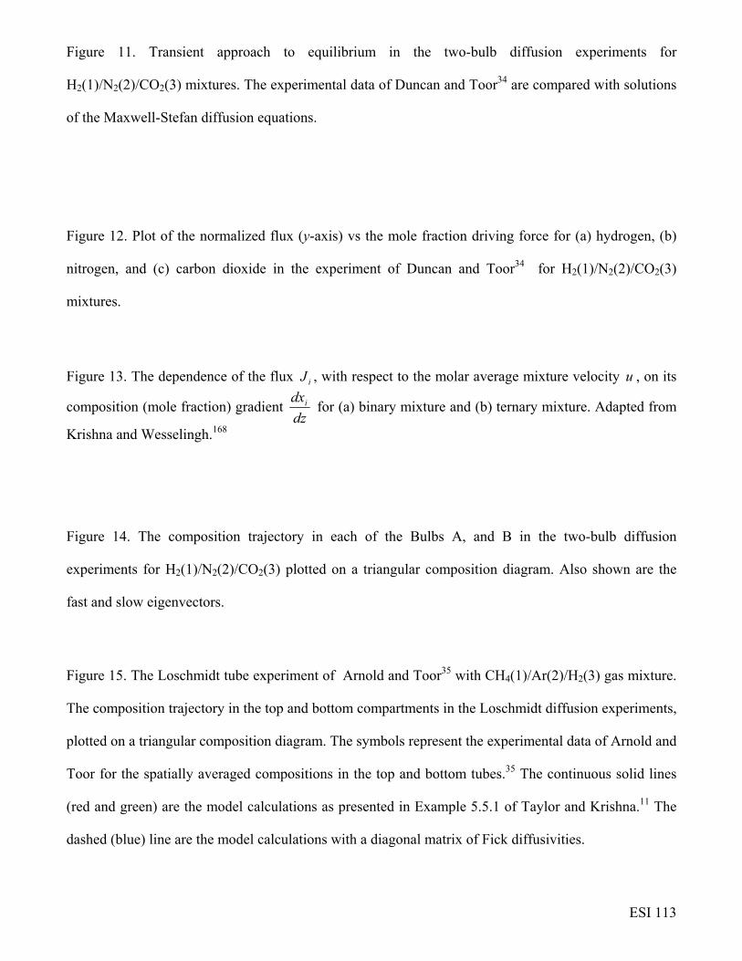
ESI 113

Figure 11. Transient approach to equilibrium in the two-bulb diffusion experiments for

H2(1)/N2(2)/CO2(3) mixtures. The experimental data of Duncan and Toor34 are compared with solutions

of the Maxwell-Stefan diffusion equations.

Figure 12. Plot of the normalized flux (y-axis) vs the mole fraction driving force for (a) hydrogen, (b)

nitrogen, and (c) carbon dioxide in the experiment of Duncan and Toor34 for H2(1)/N2(2)/CO2(3)

mixtures.

Figure 13. The dependence of the flux iJ , with respect to the molar average mixture velocity u , on its

composition (mole fraction) gradient dz

dxi for (a) binary mixture and (b) ternary mixture. Adapted from

Krishna and Wesselingh.168

Figure 14. The composition trajectory in each of the Bulbs A, and B in the two-bulb diffusion

experiments for H2(1)/N2(2)/CO2(3) plotted on a triangular composition diagram. Also shown are the

fast and slow eigenvectors.

Figure 15. The Loschmidt tube experiment of Arnold and Toor35 with CH4(1)/Ar(2)/H2(3) gas mixture.

The composition trajectory in the top and bottom compartments in the Loschmidt diffusion experiments,

plotted on a triangular composition diagram. The symbols represent the experimental data of Arnold and

Toor for the spatially averaged compositions in the top and bottom tubes.35 The continuous solid lines

(red and green) are the model calculations as presented in Example 5.5.1 of Taylor and Krishna.11 The

dashed (blue) line are the model calculations with a diagonal matrix of Fick diffusivities.

ESI 114

Figure 16. (a) The Loschmidt tube experiment of Arnold and Toor35 on the transient approach to

equilibrium for CH4(1)/Ar(2)/H2(3) gas mixtures. The plotted data are spatially averaged compositions

in the top and bottom compartments. (b) Equilibration trajectories in composition space, followed in the

two tubes. The dashed line represents the trajectory predicted by uncoupled Fickian formulation.

Figure 17.Transient approach to equilibrium in the Loschmidt tube experiment of Arnold and Toor35

with CH4(1)/Ar(2)/H2(3) gas mixture.

Figure 18. Composition trajectories for O2(1)/N2(2)/He(3) gas mixture diffusing from Left compartment

(O2 = 20 %; He = 80 %) into air contained in the Right compartment (O2 = 20 %; N2 = 80 %).

Figure 19. Transient equilibration of O2, for O2(1)/N2(2)/He(3) gas mixture diffusion, monitored at the

position z = -0.5 m.

Figure 20. Condensation of an azeotropic mixture of 2-propanol(1)/water(2) in the presence of an inert

gas such as nitrogen (3) results in a condensate which is richer in water than the azeotrope.

Figure 21. (a) Liquid/liquid phase equilibrium for methanol(1)/n-hexane (2) mixtures exhibiting with

UCST at 308 K. The calculations of the binodal curve use NRTL parameters from Clark and Rowley.40

(b) Liquid/liquid phase equilibrium for triethylamine (1) – water (2) mixture exhibiting LCST at 291.5

ESI 115

K. These are experimental data for the binodal and spinodal curves are taken from Counsell et al.169,

Kohler and Rice,170 and Vitagliano et al.42 (c) Liquid-liquid equilibrium for n-hexane (1)/ nitrobenzene

(2) mixtures with Tc = UCST = 292.56 K.49

Figure 22. (a) Calculations of (a) free energy, RT

G, (b) first derivative,

1

1

x

G

RT ∂∂

, and (c) second

derivative, 21

21

x

G

RT ∂∂

for methanol – n-hexane mixtures at various temperatures in the range 260 K – 320

K using NRTL parameters from Clark and Rowley.40 (d) Binodal and Spinodal curves, determined from

(a), (b), and (c).

Figure 23. (a) Calculations of the thermodynamic correction factor Γ for methanol – n-hexane mixtures

at 303.15 K, 305.65 K, 307.75 K, 310.65 K, and 313.15 K using NRTL parameters from Table 4. (b)

Experimental data of Clark and Rowley40 for Fick diffusivities, D12, for methanol – n-hexane mixtures

at 303.15 K, 305.65 K, 307.75 K, 310.65 K, and 313.15 K. The two sets of Figures are presented with

both linear and logarithmic scales on the y-axes.

Figure 24. Comparison of the experimental data of Clark and Rowley40 for Fick diffusivities, D12, for

methanol – n-hexane mixtures at (a) 303.15 K, (b) 305.65 K, (c) 307.75 K, (d) 310.65 K, and (e) 313.15

K with corresponding MD simulation results of Krishna and van Baten23 for the corresponding Fick and

M-S diffusivities.

ESI 116

Figure 25. Comparison of the experimental data of Clark and Rowley40 for Fick diffusivities, D12, with

the M-S diffusivities for methanol(1)/n-hexane (2) mixtures, obtained by correcting for the

thermodynamic factor Γ

= 1212

DÐ . The thermodynamic factor is calculated using NRTL parameters from

Table 4. The Onsager coefficients L12 calculated using equation (43). Also shown are the calculations

using the Vignes interpolation formula (48).

Figure 26. (a) Experimental data of Haase and Siry41 for the temperature dependence of the Fick

diffusivities, D12, for triethylamine(1)/water(2) mixtures, measured at the critical composition x1 =

0.073. (b) Thermodynamic correction factor Γ for triethylamine(1)/water(2) mixtures at temperatures T

= 277.15 K, T = 283.15, and T = 291.15 K; these plots are based on the data of D’Agostino et al.171

Figure 27. (a) Liquid/liquid phase equilibrium for triethylamine (1) – water (2) mixture exhibiting

LCST at 291.5 K. The experimental data for the binodal and spinodal curves are taken from Counsell et

al.,169 Kohler and Rice,170 and Vitagliano et al.42 (b) Experimental data of Vitagliano et al.42 for Fick

diffusivities, D12, for triethyamine(1)/water(2) mixtures, measured at two different temperatures 292.15

K, and 293.15 K, for various compositions on either side of the spinodal curves in (a).

Figure 28. Fick diffusivity of (a) urea, and (b) glycine in aqueous solutions function of molar

concentration of solute. Experimental data of Myerson and Senol,43 and Chang and Myerson.44

Figure 29. Fick diffusivity of n-hexane (1) / nitrobenzene (2) mixtures as a function of (T – Tc) with Tc

= UCST = 292.56 K. Experimental data of Matos Lopes et al.,48 Haase and Siry,41 and Wu et al.49

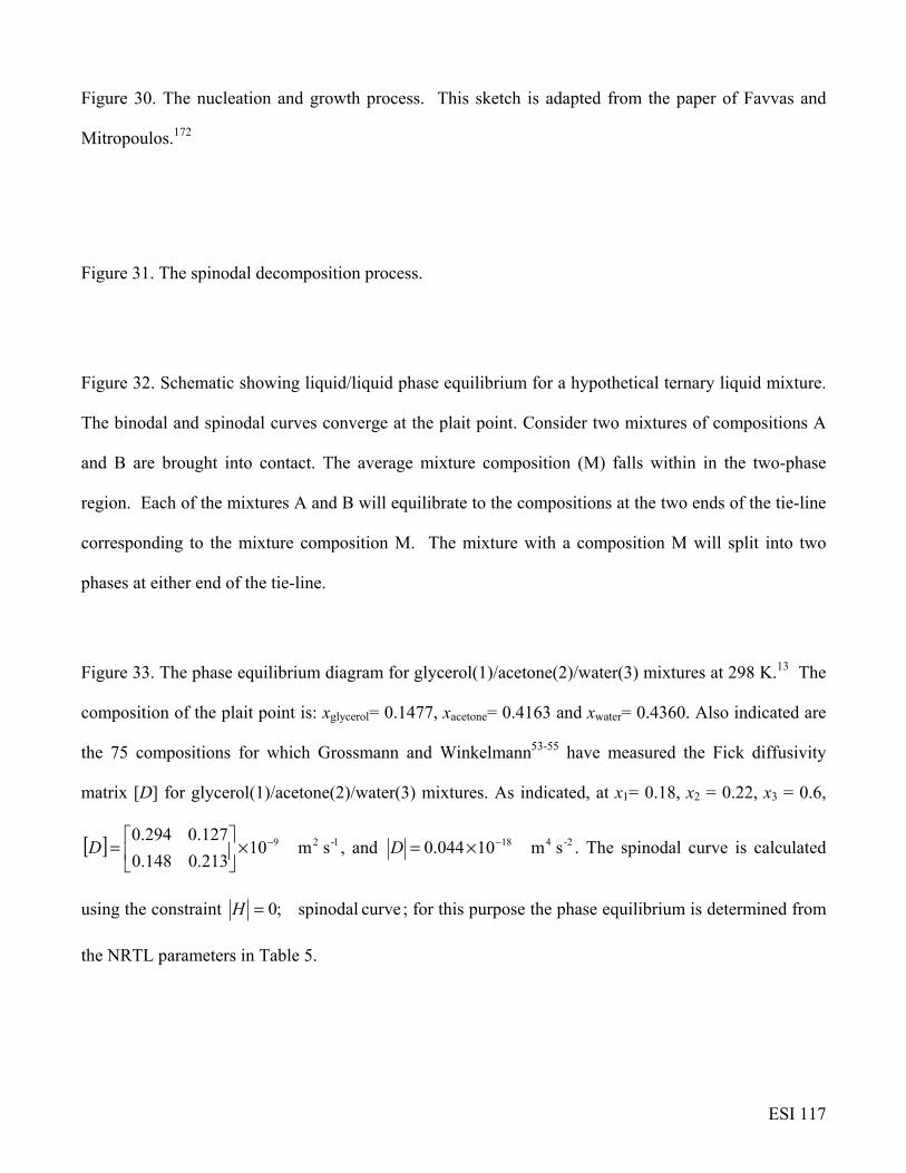
ESI 117

Figure 30. The nucleation and growth process. This sketch is adapted from the paper of Favvas and

Mitropoulos.172

Figure 31. The spinodal decomposition process.

Figure 32. Schematic showing liquid/liquid phase equilibrium for a hypothetical ternary liquid mixture.

The binodal and spinodal curves converge at the plait point. Consider two mixtures of compositions A

and B are brought into contact. The average mixture composition (M) falls within in the two-phase

region. Each of the mixtures A and B will equilibrate to the compositions at the two ends of the tie-line

corresponding to the mixture composition M. The mixture with a composition M will split into two

phases at either end of the tie-line.

Figure 33. The phase equilibrium diagram for glycerol(1)/acetone(2)/water(3) mixtures at 298 K.13 The

composition of the plait point is: xglycerol= 0.1477, xacetone= 0.4163 and xwater= 0.4360. Also indicated are

the 75 compositions for which Grossmann and Winkelmann53-55 have measured the Fick diffusivity

matrix [D] for glycerol(1)/acetone(2)/water(3) mixtures. As indicated, at x1= 0.18, x2 = 0.22, x3 = 0.6,

[ ] 1-29 s m10213.0148.0

127.0294.0 −×

=D , and -2418 s m10044.0 −×=D . The spinodal curve is calculated

using the constraint curve spinodal;0=H ; for this purpose the phase equilibrium is determined from

the NRTL parameters in Table 5.

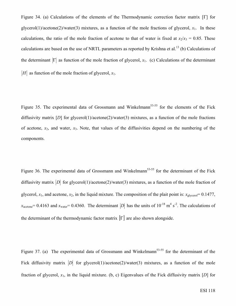
ESI 118

Figure 34. (a) Calculations of the elements of the Thermodynamic correction factor matrix [Γ] for

glycerol(1)/acetone(2)/water(3) mixtures, as a function of the mole fractions of glycerol, x1. In these

calculations, the ratio of the mole fraction of acetone to that of water is fixed at x2/x3 = 0.85. These

calculations are based on the use of NRTL parameters as reported by Krishna et al.13 (b) Calculations of

the determinant Γ as function of the mole fraction of glycerol, x1. (c) Calculations of the determinant

H as function of the mole fraction of glycerol, x1.

Figure 35. The experimental data of Grossmann and Winkelmann53-55 for the elements of the Fick

diffusivity matrix [D] for glycerol(1)/acetone(2)/water(3) mixtures, as a function of the mole fractions

of acetone, x2, and water, x3. Note, that values of the diffusivities depend on the numbering of the

components.

Figure 36. The experimental data of Grossmann and Winkelmann53-55 for the determinant of the Fick

diffusivity matrix D for glycerol(1)/acetone(2)/water(3) mixtures, as a function of the mole fraction of

glycerol, x1, and acetone, x2, in the liquid mixture. The composition of the plait point is: xglycerol= 0.1477,

xacetone= 0.4163 and xwater= 0.4360. The determinant D has the units of 10-18 m4 s-2. The calculations of

the determinant of the thermodynamic factor matrix [ ]Γ are also shown alongside.

Figure 37. (a) The experimental data of Grossmann and Winkelmann53-55 for the determinant of the

Fick diffusivity matrix D for glycerol(1)/acetone(2)/water(3) mixtures, as a function of the mole

fraction of glycerol, x1, in the liquid mixture. (b, c) Eigenvalues of the Fick diffusivity matrix [D] for

ESI 119

glycerol(1)/acetone(2)/water(3) mixtures, as a function of the mole fraction of glycerol, x1, and acetone,

x2, in the liquid mixture.

Figure 38. (a) The ratios D12/D11, and D21/D22 of the Fick diffusivity matrix [D] for

glycerol(1)/acetone(2)/water(3) mixtures plotted as a function of the determinant D . These

experimental data are from Grossmann and Winkelmann53-55 (b) The ratios D12/D11, and Γ12/Γ11 plotted

as a function of the determinant D .

Figure 39. The ratio 2/1

2/1

Γ

D glycerol(1)/acetone(2)/water(3) mixtures, plotted (a) as a function of the

mole fractions of acetone, x2, and water x3 and (b) only as a function of the mole fraction of acetone, x2.

Figure 40. Experimental data of Vitagliano et al.56 for Fick diffusivity matrix [D] of

water(1)/chloroform(2)/acetic-acid(3) mixtures at six different compositions. The measured values of

the Fick matrix [D], in units of 10-9 m2 s-1, are indicated. The composition of the plait point is x1 =

0.375, x2= 0.262, x3= 0.363. The binodal curve is from the experimental data of Othmer and Ku.157 The

spinodal curve is obtained from the criterion of phase stability; the UNIQUAC parameters are provided

in Table 6.

Figure 41. Experimental data of Buzatu et al.57 for Fick diffusivity matrix [D] of

water(1)/chloroform(2)/acetic-acid(3) mixtures at six different compositions. The measured values of

the Fick matrix [D], in units of 10-9 m2 s-1, are indicated. The composition of the plait point is x1 =

0.375, x2= 0.262, x3= 0.363.

ESI 120

Figure 42. (a) Plot of the determinant D that has the units of 10-18 m4 s-2 as a function of (1- x3) for

water(1)/chloroform(2)/acetic-acid(3) mixtures. (b) Plot of the determinant Γ as a function of (1- x3)

for water(1)/chloroform(2)/acetic-acid(3) mixtures. (c) The ratio 2/1

2/1

Γ

D plotted as a function of (1- x3).

(d) The ratios Γ12/ Γ11, and Γ21/ Γ22 plotted as a function of the determinant Γ . (e) The ratios D12/D11,

and D21/D22 of the Fick diffusivity matrix [D] for water(1)/chloroform(2)/acetic-acid(3) mixtures plotted

as a function of the determinant D . The experimental data are from Vitagliano et al.56 and Buzatu et

al.57

Figure 43. (a) Experimental data of Clark and Rowley58 for the determinant of the Fick diffusivity

matrix D for water(1)/2-propanol(2)/cyclohexane(3) mixtures as (T – Tc) where T is the temperature at

which the diffusivities are measured, with Tc = 303.67 K. The elements of the Fick matrix of

diffusivities were measured at a constant composition of the plait point at 303.67 K: x1 = 0.367, x2=

0.389, x3= 0.244. The measured values of the Fick matrix [D], in units of 10-10 m2 s-1, are also indicated;

the corresponding values of the determinant D has the units of 10-18 m4 s-2. (b) Data of Battler et al.173

for the binodal curves at T = 293.15 K, 303.15 K, and 323.15 K.

Figure 44. Phase equilibrium diagram for acetone/water/ethylacetate mixtures at 293 K. The binodal

curve data is from Haeberl and Blass.61 The spinodal curve is obtained from the criterion of phase

stability; the UNIQUAC parameters are provided Table 7. Also indicated are the six experimental

values of of Pertler59 for the elements of the Fick diffusivity matrix in the ethylacetate-rich region of the

ESI 121

phase diagram; these values correspond to the component numbering:

acetone(1)/water(2)/ethylacetate(3). The phase diagram is plotted in mass fractions.

Figure 45. Experimental data of Pertler59 for the elements of the Fick diffusivity matrix in the water-

rich region of the phase diagram; these values correspond to the component numbering:

acetone(1)/ethylacetate(2)/water(3). The phase diagram is plotted in mass fractions.

Figure 46. Transient inter-diffusion in a diffusion couple consisting of water(1)/chloroform(2)/acetic-

acid(3) mixtures. The compositions of the two mixtures in the left and right chambers are indicated;

both initial compositions and the final equilibrated compositions are in the homogeneous single phase

region. The transient approach to equilibrium is plotted against the dimensionless coordinate tD

z

ref4

where the value of the reference diffusivity 910−=refD m2 s-1. The values of the Fick diffusivity matrix

is [ ] 2-4181-29 s m10164.0;s m10939.0344.0

368.0309.0 −− ×=×

= DD , corresponding to the fifth data set

of Vitagliano et al.56

Figure 47. Equilibration trajectories in glycerol(1)/acetone(2)/water(3) mixtures at 298 K. The

equilibration trajectories were simulated for two cases, with two different equilibrium compositions: (a)

x1= 0.18, x2 = 0.22, x3 = 0.6, and (b) x1= 0.1, x2 = 0.432, x3 = 0.468. The Fick diffusivity matrix for

these two simulations are obtained from the experimental data of Grossmann and Winkelmann53-55;

these are indicated.

ESI 122

Figure 48. (a) Equilibration trajectories in glycerol(1)/acetone(2)/water(3) mixtures at 298 K for the

equilibrium composition x1= 0.1, x2 = 0.432, x3 = 0.468. The plot is in 2D composition space. (b) For the

trajectory in (a), the transient approach to equilibrium of each component is plotted against the

dimensionless coordinate tD

z

ref4 where the value of the reference diffusivity 910−=refD m2 s-1. The

Fick diffusivity matrix for this simulation is indicated in Figure 47. (c) Equilibration trajectories plotted

in 2D activity space. (d) Transient equilibration of glycerol, expressed in both mole fractions and

activities.

Figure 49. (a) Equilibration trajectories in glycerol(1)/acetone(2)/water(3) mixtures at 298 K for the

equilibrium composition x1= 0.18, x2 = 0.22, x3 = 0.6. The plot is in 2D composition space. The Fick

diffusivity matrix for this simulation is indicated in Figure 47. (b) Equilibration trajectories plotted in

2D activity space. (c) Transient equilibration of glycerol, expressed in both mole fractions and

activities, plotted against the dimensionless coordinate tD

z

ref4 where the value of the reference

diffusivity 910−=refD m2 s-1.

Figure 50. Transient inter-diffusion in water(1)/chloroform(2)/acetic-acid(3) mixtures. The

compositions of the two mixtures in the left and right chambers are indicated; both initial compositions

and the final equilibrated compositions are in the homogeneous single phase region, at a tangent to the

binodal curve. The transient approach to equilibrium is plotted against the dimensionless coordinate

tD

z

ref4 where the value of the reference diffusivity 910−=refD m2 s-1. The values of the Fick

ESI 123

diffusivity matrix is [ ] 0;s m10161.037.0

40.092.0 1-29 =×

= − DD , corresponding to those determined by

Vitagliano et al.56 at the plait point.

Figure 51. Experimental data for the equilibration paths for glycerol(1)/acetone(2)/water(3) mixture

measured in a stirred Lewis cell by Krishna et al.60 The data for the acetone rich phase are shown by the

green squares. The data for glycerol-rich phase are shown by red circles. The mixture composition

indicated by M on the dashed line connecting the two initial compositions in the acetone-rich and

glycerol-rich regions separates into two liquid phases with compositions at either end of the tie-line as

indicated. The values of the Fick diffusivity matrices used in the simulations of the equilibration

trajectories are also indicated.

Figure 52. Comparison of experimental data (red circles) for the equilibration paths in the glycerol-rich

phase for the system glycerol(1)/acetone(2)/water(3) mixture with the model calculations shown by the

continuous solid red lines.

Figure 53. Comparison of experimental data (green squares) for the equilibration paths in the acetone-

rich phase for the system glycerol(1)/acetone(2)/water(3) mixture with the model calculations shown by

the continuous solid green lines.

ESI 124

Figure 54. Equilibration trajectory followed in acetone(1)/ethylacetate(2)/water(3) mixtures at 293 K.

Two mixtures of compositions (in mass tractions) ω1=0.01, ω2=0.01, ω3=0.98, and

ω1=0.17, ω2=0.1, ω3=0.73 are allowed to equilibrate to yield the final equilibrated value

ω1=0.09, ω2=0.055, ω3=0.855. The values of the Fick diffusivity used in the calculations corresponds to

the third point in the water-rich data set of Pertler59: [ ] 1-29 s m10764.0316.0

287.0179.0 −×

−=D . Also shown

in the inset are the experimental data points obtained by Haeberl and Blass.61

Figure 55. Experimental data of Krishna et al.60 on the equilibration paths for the system

glycerol(1)/acetone(2)/water(3) mixture. The initial compositions in the two compartments lie on the

tangent to the plait point (composition: xglycerol= 0.1477, xacetone= 0.4163, xwater= 0.4360) parallel to the

tie lines.

Figure 56. Phase equilibrium diagram for the ternary mixture of trans-anethol/ethanol/water. The

binodal curve data is from Sitnikova et al.65 Also shown are the typical composition of Ouzo that is

three component mixture of ethanol (≈45 vol%), water (55 vol%) and an essential oil called trans-

anethol (≈ 0.1%).

Figure 57. Equlibration trajectories followed on addition of water to Ouzo.

ESI 125

Figure 58. Trajectories followed during equilibration of homogenous mixtures of different compositions

for the system toluene(1)/ethanol(2)/water(3). The NRTL parameters for toluene(1)/ethanol(2)/water(3)

are provided in Table 8. Please note that the compositions are plotted in mass fraction space.

Figure 59. Transient inter-diffusion in a diffusion couple consisting of water(1)/chloroform(2)/acetic-

acid(3) mixtures. The values of the Fick diffusivity matrix is

[ ] 2-4181-29 s m10164.0;s m10939.0344.0

368.0309.0 −− ×=×

= DD , corresponding to the fifth data set of

Vitagliano et al.56

Figure 60. The diffusion trajectories followed during equilibration of water(1)/chloroform(2)/acetic-

acid(3) mixtures. Also shown by the dashed lines are the “fast” and “slow” eigenvectors. The values of

the Fick diffusivity matrix is [ ] 2-4181-29 s m10164.0;s m10939.0344.0

368.0309.0 −− ×=×

= DD ,

corresponding to the fifth data set of Vitagliano et al.56

Figure 61. Equilibration trajectory followed by a small perturbation in acetone(1)/water(2)/

ethylacetate(3) mixtures at 293 K. Two mixtures of compositions (in mass tractions)

ω1=0.17, ω2=0.05, ω3=0.78, and ω1=0.23, ω2=0.05, ω3=0.72 are allowed to equilibrate to yield the final

equilibrated value ω1=0.2, ω2=0.05, ω3=0.75. The values of the Fick diffusivity used in the calculations

corresponds to the sixth point in the ethylacetate-rich data set of Pertler59:

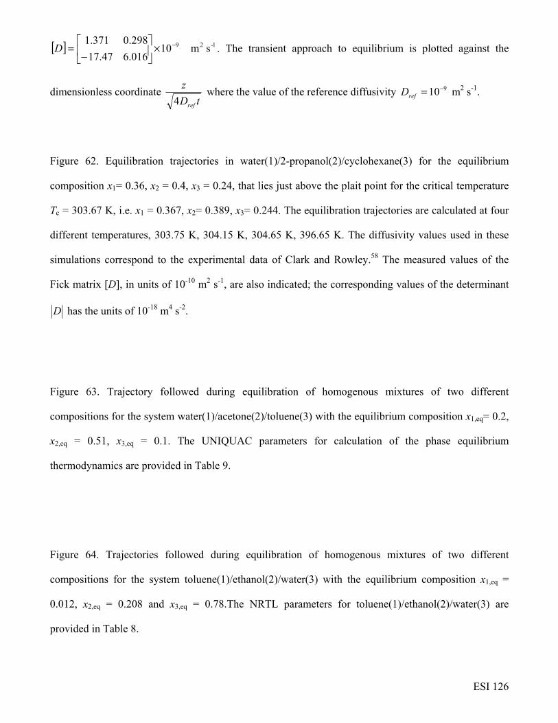
ESI 126

[ ] 1-29 s m10016.647.17

298.0371.1 −×

−

=D . The transient approach to equilibrium is plotted against the

dimensionless coordinate tD

z

ref4 where the value of the reference diffusivity 910−=refD m2 s-1.

Figure 62. Equilibration trajectories in water(1)/2-propanol(2)/cyclohexane(3) for the equilibrium

composition x1= 0.36, x2 = 0.4, x3 = 0.24, that lies just above the plait point for the critical temperature

Tc = 303.67 K, i.e. x1 = 0.367, x2= 0.389, x3= 0.244. The equilibration trajectories are calculated at four

different temperatures, 303.75 K, 304.15 K, 304.65 K, 396.65 K. The diffusivity values used in these

simulations correspond to the experimental data of Clark and Rowley.58 The measured values of the

Fick matrix [D], in units of 10-10 m2 s-1, are also indicated; the corresponding values of the determinant

D has the units of 10-18 m4 s-2.

Figure 63. Trajectory followed during equilibration of homogenous mixtures of two different

compositions for the system water(1)/acetone(2)/toluene(3) with the equilibrium composition x1,eq= 0.2,

x2,eq = 0.51, x3,eq = 0.1. The UNIQUAC parameters for calculation of the phase equilibrium

thermodynamics are provided in Table 9.

Figure 64. Trajectories followed during equilibration of homogenous mixtures of two different

compositions for the system toluene(1)/ethanol(2)/water(3) with the equilibrium composition x1,eq =

0.012, x2,eq = 0.208 and x3,eq = 0.78.The NRTL parameters for toluene(1)/ethanol(2)/water(3) are

provided in Table 8.

ESI 127

Figure 65. Trajectory followed during equilibration of homogenous mixtures of two different

compositions for the system water(1)/caprolactam(2)/toluene(3) for the equilibrium composition x1,eq =

0.64, x2,eq = 0.2725 and x3,eq = 0.0875. The UNIQUAC parameters for calculation of the phase

equilibrium thermodynamics are provided in Table 10.

Figure 66. Trajectory followed during equilibration of homogenous mixtures of two different

compositions for the system water(1)/caprolactam(2)/benzene (3) for the equilibrium composition x1=

0.125, x2 = 0.165, x3 = 0.71. The UNIQUAC parameters for calculation of the phase equilibrium

thermodynamics are provided in Table 11.

Figure 67. Trajectory followed during equilibration of homogenous mixtures of two different

compositions for the system for toluene(1)/propionic-acid (2)/water(3) for the equilibrium composition

x1,eq = 0.475, x2,eq = 0.4 and x3,eq = 0.285. The UNIQUAC parameters for calculation of the phase

equilibrium thermodynamics are provided in Table 12.

Figure 68. Trajectory followed during equilibration of homogenous mixtures of two different

compositions for the system for ethylacetate(1)/propionic-acid(2)/water(3) for the equilibrium

composition x1,eq = 0.675, x2,eq = 0.13 and x3,eq = 0.195. The UNIQUAC parameters for calculation of

the phase equilibrium thermodynamics are provided in Table 13.

ESI 128

Figure 69. Diffusion trajectories during the immersion precipitation process for membrane preparation;

adapted from the papers of van den Berg and Smolders,71 and Reuvers and Smolders.72 A 10% solution

of Cellulose Acetate (CA) in acetone is immersed in a bath of pure water. The transient equilibration

trajectories at three different times, t =10 s, t = 25 s, and t = 50 s are depicted.

Figure 70. (a) Effective diffusivity of water and acetone in maltodextrin, and coffee extract solutions as

a function of wt% water content. (b) Ratio of diffusivities of acetone and water in aqueous maltodextrin,

and coffee extract solutions as function of wt % water content. The graphs are re-drawn using data from

Coumans et al.76

Figure 71. Experimental data of Darken17 for inter-diffusion between the left and right austenite bars

consisting of C/Si/Fe mixtures. The wt% of each component is measured on either side of the Matano

plane, measured at t = 13 days after the start of the experiment are shown. The calculations of the

coupled diffusion model are based on the Fick diffusivity matrix determined by Kirkaldy for this

experiment.78

Figure 72. Transient equilibration of a diffusion couple consisting of Cu(1)/Ag(2)/Au(3) mixtures. The

atom fractions at equilibrium are x1= 0.475, x2 = 0.175, x3 = 0.35. The trajectories are calculated with

the values of the Fick diffusivity matrix [ ] 1-214 s m101.38.1

11.13.2 −×

=D . The transient approach to

equilibrium is plotted against the dimensionless coordinate tD

z

ref4 where the value of the reference

diffusivity 1410−=refD m2 s-1.

ESI 129

Figure 73. (a) Experimental data of Varshneya and Cooper79 for inter-diffusion between the left and

right slabs consisting of K2O/SrO/SiO2 mixtures. The wt% of each component is measured on either

side of the Matano plane, measured at t = 4.55 h after the start of the experiment are shown. (b)

Trajectories in 3D composition space.

Figure 74. Experimental data of Vielzeuf and Saúl80 for inter-diffusion in a diffusion couple consisting

of Fe/Mg/Ca mixtures. The atom % of each component is measured on either side of the Matano plane,

measured at t = 100 h after the start of the experiment are shown.

Figure 75. (a) Experimental data of Vielzeuf and Saúl80 for inter-diffusion between the left and right

slabs containing Fe/Mg/Ca mixtures. The atom % of each component is measured on either side of the

Matano plane, measured at t = 100 h after the start of the experiment are shown as function of the

distance. (b) Equilibration trajectories in composition space. The dashed line represents the trajectory

predicted by uncoupled Fickian formulation.

Figure 76. Schematic showing vapor/liquid contacting on a distillation tray.

Figure 77. (a) Schematic of a laboratory-scale distillation column used in the experiments of Springer et

al.84, 86 which includes a total condenser (1), a partial reboiler (12), 10 bubble-cap trays (2-11), and 13

draw-off faucets, 9 for vapor samples and 4 for liquid samples. (b) Ethanol driving force ( )Eyy −*2 on

ESI 130

each stage for the system water(1)/ethanol(2)/acetone(3). (c) Murphree component efficiencies for the

system water(1)/ethanol(2)/acetone(3).

Figure 78. (a) Residue curve map for the water(1)/ethanol(2)/acetone(3) system, showing a straight-line

distillation boundary and a binary minimum-boiling azeotrope between water and ethanol (large green

circle). The pure component boiling points are indicated in green letters: water = 373.2 K; ethanol =

351.6 K; acetone = 329.7 K; water/ethanol azeotrope = 351.4 K. (b, c) Experimental data for (b) Run

T2-6, and (c) T2-26 of Springer et al.86 (blue circles) showing the column composition trajectories for

the water(1)/ethanol(2)/acetone(3) system in the column operating at total reflux implying ii yx = . Also

shown in (b, c) are the simulation results showing the trajectories calculated by the Equilibrium (EQ)

stage model (continuous green line, 1,3,2,1 === MVMVMV EEE ) and the Non-Equillibrium (NEQ) stage

model (continuous red line, properly accounting for the resistances to transfer in both vapor and liquid

phases, resulting in MVMVMV EEE ,3,2,1 ≠≠ ). The solid black line is the distillation boundary.

Figure 79. Experimental data of Springer et al.85 (red circles) for composition trajectories for distillation

of water(1)/acetone(2)/toluene(3) mixtures. The grey shaded areas represent the region in which liquid–

liquid phase splitting occurs. The pure component boiling points are indicated in green letters: water =

373.2 K; toluene = 384 K; acetone = 329.7 K; water/toluene azeotrope = 358 K.

Figure 80. Diffusion in mixed ion systems. Experimental data of Vinograd and McBain93 for ionic

diffusivities of H+, Ba++, and Cl- in a two-compartment diffusion cell. The continuous solid lines are the

ESI 131

calculations using the Nernst-Planck equation; for further computational details see Example 2.4.2 of

Taylor and Krishna.11

Figure 81. External mass transfer limited transfer rates to and from ion-exchange particles are direction

dependent. Experimental data of Kraaijeveld and Wesselingh.94

Figure 82. Experimental data of Yang and Pintauro95 for the transient concentrations of H+, Na+, and

Cs+ in the salt and acid compartments that are separated by a Nafion cation exchange membrane.

Figure 83. Water transport across polyamide-based Reverse Osmosis (RO) membrane. Adapted from

Wesselingh and Krishna.25

Figure 84. Examples of one-dimensional (1D) channel structures: AFI, MgMOF-74, and MIL-53(Cr)-lp,

BTP-COF, and Fe2(BDP)3.

Figure 85. Examples of 1D channel structures with side pockets: MOR and FER.

Figure 86. Examples of structures consisting of intersecting channels: MFI, and Zn(bdc)dabco.

Figure 87. Structures consisting of cages separated by narrow windows: LTA, CHA, DDR, and ZIF-8.

ESI 132

Figure 88. “Open” structures that consist of cages separated by large windows: IRMOF-1, CuBTC, and

FAU.

Figure 89. PSA process for production of purified N2 by separation of O2(1)/N2(2) mixture in a fixed

bed adsorber packed with LTA-4A operating at a total pressure of 200 kPa and 298 K. The simulation

details are available in the Supplementary Material accompanying the article by Krishna.104

Figure 90. Schematic of membrane permeation device. Typically, the micro-porous crystalline layer

has a thickness of 25 – 50 μm.

Figure 91. (a) Thermodynamic factor Γi, for single-site Langmuir isotherm, plotted as a function of the

fractional occupancy. (b) Inverse thermodynamic factor iΓ1 , plotted as a function of the fractional

occupancy.

Figure 92. Transient adsorption and desorption profiles for C2H6 in LTA-4A zeolite at 298 K.

Experimental data of Garg and Ruthven.123

ESI 133

Figure 93. Experimental data of Niessen and Karge124 for transient adsorption/desorption of p-xylene in

MFI zeolite (H-ZSM-5) at 375 K.

Figure 94 Configurational-Bias Monte Carlo (CBMC) simulations117 of (a) Unary adsorption isotherms,

and (b) Inverse thermodynamic factors for adsorption of methanol, and ethanol in ZIF-8. (c, d)

Experimental data of Chmelik et al.130 for the unary Fick and M-S diffusivities of methanol, and ethanol

in ZIF-8.

Figure 95. Experimental data of Habgood135 on transient uptake of N2(1)/CH4(2) mixture within LTA-

4A crystals, exposed to binary gas mixtures at 194 K and partial pressures p1 =50.9 kPa; p2 = 49.1 kPa.

Figure 96. (a) Elements of the matrix of thermodynamic factors Γij for N2(1)/CH4(2) mixture adsorption

in LTA-4A crystals, exposed to equimolar binary gas mixtures. The data is plotted as a function of the

total mixture loading, qt. (b) Elements of the matrix of thermodynamic factors Γij calculated from the

transient uptake simulations. The data is plotted as a function of t1/2. (c) Calculations of 212111 qq Γ+Γ ,

and 222121 qq Γ+Γ as a function of t1/2. For the calculations on (a), (b), and (c), we use the mixed-gas

Langmuir model. The pure component isotherms were fitted to the experimental data using the single-

site Langmuir parameters: N2: q1,sat = 3.6 mol kg-1; b1 = 9.4×10-5 Pa-1; CH4: q2,sat = 3.6 mol kg-1; b1 =

2.08×10-4 Pa-1.

ESI 134

Figure 97. Comparison of the Maxwell-Stefan model calculations with the experimental data of

Habgood135 on transient uptake of N2(1)/CH4(2) mixture within LTA-4A crystals, exposed to binary gas

mixtures at 194 K and partial pressures p1 =50.9 kPa; p2 = 49.1 kPa. Maxwell-Stefan diffusivities:

21 crÐ = 1.56×10-5 s-1; 2

2 crÐ = 7.2×10-9 s-1. The continuous solid lines are the calculations using

Equation (136). The dashed lines are the calculations using uncoupled flux equation (139).

Figure 98. (a) Simulations of the transient desorption process for N2(1)/CH4(2) mixture in LTA-4A

crystals, exposed to binary gas mixtures at 194 K. The initial crystal is brought to equilibrium by

exposure to gas phase partial pressures p1 =50.9 kPa; p2 = 49.1 kPa. At time t = 0, the bulk gas is

exposed to conditions such that p1 = p2 = 0. (b) Comparison of the composition trajectories for the

adsorption (green line) and desorption cycles (red line) for transient adsorption/desorption of

N2(1)/CH4(2) mixture within LTA-4A crystals, exposed to binary gas mixtures at 194 K. Both sets of

simulations include thermodynamic coupling effects.

Figure 99. PSA process for separation of 10/90 N2(1)/CH4(2) mixture in a fixed bed adsorber packed

with LTA-4A operating at a total pressure of 100 kPa and 194 K.

Figure 100. (a, b) Experimental data of Majumdar et al.134 for transient uptake of (a) 10/90, and (b)

50/50 mixtures of N2(1)/CH4(2) mixtures in Ba-ETS-4 at 283 K and total pressure of 0.7 MPa. Note that

the y-axes represent the fractional uptake of each component; this is obtained by dividing each of the

ESI 135

component loadings by the final equilibrated loading within the crystal. The experimentally observed

overshoots for N2 result from thermodynamic coupling effects.

Figure 101. Transient uptake of O2(1)/N2(2) mixture in LTA-4A crystals exposed to a total pressure of

200 kPa and 298 K. The transient uptake simulations use Equation (136) taking 22 cO rÐ =2×10-3 s-1;

22 NO ÐÐ =100. The single-site Langmuir parameters for pure component isotherms are: O2: q1,sat = 1.91

mol kg-1; b1 = 5.65×10-7 Pa-1; N2: q2,sat = 1.91 mol kg-1; b2 = 1.13×10-6 Pa-1. The ratio b2/b1 = 2. Further

simulation details are available in the Supplementary Material accompanying the article by Krishna.104

Figure 102. (a) The experimental data of Chen et al.138 for transient uptake of O2(1)/N2(2) mixture in

carbon molecular sieve (CMS) at 300 K exposed to binary gas mixtures at partial pressures p1 =109.6

kPa; p2 = 432.56 kPa. The continuous solid lines are transient uptake simulations use Equation (136)

taking 22 cO rÐ =3.5×10-4 s-1; 2

2 cN rÐ =9.5×10-6 s-1; 22 NO ÐÐ =36.8. The single-site Langmuir

parameters for pure component isotherms are: O2: q1,sat = 1.9 mol kg-1; b1 = 1.45×10-6 Pa-1; N2: q2,sat =

1.4 mol kg-1; b2 = 1.5×10-6 Pa-1. (b) Comparison of the adsorption/desorption cycles in composition

space.

Figure 103. Experimental data of Carlson and Dranoff139 on the fractional approach to equilibrium

during the co-adsorption of methane and ethane in LTA-4A zeolite. The experimentally observed

overshoot for methane result from thermodynamic coupling effects.

ESI 136

Figure 104. Simulations of transient uptake of C3H6(1)/C3H8(2) within crystals of ZIF-8. The

simulations for ZIF-8 are at 303 K using the isotherm parameters specified in Table 14, along with

21 crÐ = 1.5×10-2 s-1; 21 ÐÐ = 125; ratio of single-site Langmuir parameter 12 bb = 1.07. The

continuous solid lines are the calculations using Equation (136). The dashed lines are the calculations

using uncoupled flux equation (139).

Figure 105. Simulations of transient uptake of C3H6(1)/C3H8(2) within crystals of CHA. The simulations

for CHA are at 353 K and based on the data provided by Khalighi et al.141: 21 crÐ = 1.73×10-4 s-1;

21 ÐÐ = 5000; ratio of single-site Langmuir parameter 12 bb = 2.67. The continuous solid lines are

the calculations using Equation (136). The dashed lines are the calculations using uncoupled flux

equation (139).

Figure 106. Experimental data of Saint-Remi et al.142 for transient uptake of (a) ethanol/1-propanol, and

(b) methanol/1-propanol mixtures within SAPO-34, that is the structural analog of CHA zeolite. The

experimentally observed overshoot for ethanol, and methanol result from thermodynamic coupling

effects; this has been shown in the simulation results presented in the Supplementary Material

accompanying the article by Krishna.104

Figure 107. Radial profiles of the loadings of ethanol and 1-propanol within CHA crystal, for ethanol/1-

propanol mixture uptake, monitored at times t = 102 s, t = 103 s, t = 1×104 s, and t = 5×104 s.

ESI 137

Figure 108. Separation of ethanol/1-propanol mixtures in a fixed bed adsorber packed with SAPO-34.

(a) experimental uptake data reported by Saint-Remi et al.142 within the crystals of SAPO-34. (b)

Experimental data of Remy et al.143 for transient breakthroughs.

Figure 109. (a, b) Transient (a) adsorption, and (b) desorption for ethanol(1)/1-propanol(2) mixture in

CHA at 300 K. In (b) initially the crystal is equilibrated by exposing to an equimolar gas phase mixture

with partial fugacities of 1 MPa; at time t = 0, the bulk gas phase is maintained with partial fugacities of

1 kPa. In (a) the reverse scenario holds. (c) Comparison of the adsorption/desorption composition

trajectories. The mixture thermodynamics equilibrium is determined using the IAST.

Figure 110. Experimental data of Kärger and Bülow145 for transient uptake of n-heptane(1)/benzene(2)

mixture in NaX zeolite at 359 K. The experimentally observed overshoot for n-heptane result from

thermodynamic coupling effects. Also shown in the portrait or Professor Jörg Kärger who carried out

several pioneering experimental studies on diffusion that has paved the way to a better understanding of

the motion of molecules within nanoporous materials.

Figure 111. Experimental data of Niessen and Karge124, 148 for uptake of benzene(1)/ethylbenzene(2)

mixture in MFI zeolite (H-ZSM-5). The experimentally observed overshoots for benzene result from

thermodynamic coupling effects; this has been shown in the simulation results presented in the

Supplementary Material accompanying the article by Krishna.104

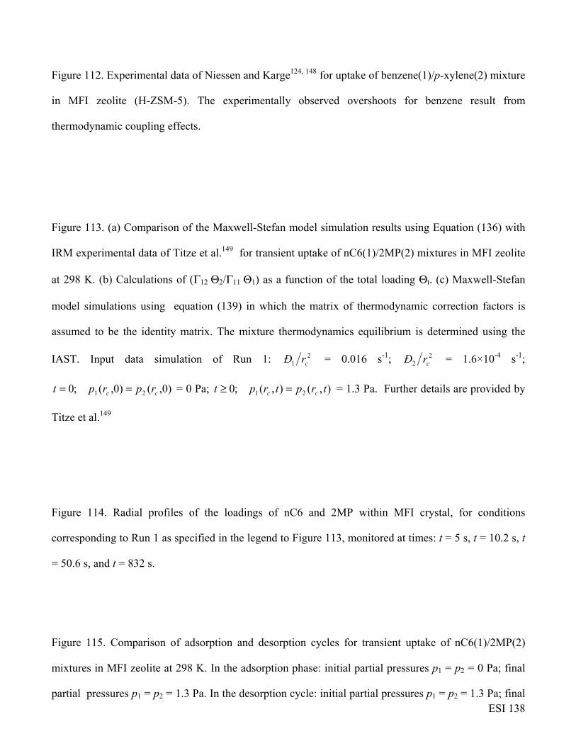
ESI 138

Figure 112. Experimental data of Niessen and Karge124, 148 for uptake of benzene(1)/p-xylene(2) mixture

in MFI zeolite (H-ZSM-5). The experimentally observed overshoots for benzene result from

thermodynamic coupling effects.

Figure 113. (a) Comparison of the Maxwell-Stefan model simulation results using Equation (136) with

IRM experimental data of Titze et al.149 for transient uptake of nC6(1)/2MP(2) mixtures in MFI zeolite

at 298 K. (b) Calculations of (Γ12 Θ2/Γ11 Θ1) as a function of the total loading Θt. (c) Maxwell-Stefan

model simulations using equation (139) in which the matrix of thermodynamic correction factors is

assumed to be the identity matrix. The mixture thermodynamics equilibrium is determined using the

IAST. Input data simulation of Run 1: 21 crÐ = 0.016 s-1; 2

2 crÐ = 1.6×10-4 s-1;

)0,()0,(;0 21 cc rprpt == = 0 Pa; ),(),(;0 21 trptrpt cc =≥ = 1.3 Pa. Further details are provided by

Titze et al.149

Figure 114. Radial profiles of the loadings of nC6 and 2MP within MFI crystal, for conditions

corresponding to Run 1 as specified in the legend to Figure 113, monitored at times: t = 5 s, t = 10.2 s, t

= 50.6 s, and t = 832 s.

Figure 115. Comparison of adsorption and desorption cycles for transient uptake of nC6(1)/2MP(2)

mixtures in MFI zeolite at 298 K. In the adsorption phase: initial partial pressures p1 = p2 = 0 Pa; final

partial pressures p1 = p2 = 1.3 Pa. In the desorption cycle: initial partial pressures p1 = p2 = 1.3 Pa; final

ESI 139

partial pressures p1 = p2 = 0 Pa. The diffusivity inputs are as indicated in the legend to Figure 113. The

continuous solid lines using Equation (136) that include thermodynamic coupling effects as described

by Titze et al.149 The dashed lines are simulations using uncoupled flux equation (139).

Figure 116. Transient adsorption/desorption kinetics for nC6/2MP mixture in MFI zeolite at 298 K. In

the desorption cycle: initial partial pressures p1 = p2 = 2 Pa; final partial pressures: p1 = p2 = 0.2 Pa. In

the adsorption cycle: initial partial pressures p1 = p2 = 0.2 Pa; final partial pressures: p1 = p2 = 2 Pa.

The mixture thermodynamics equilibrium is determined using the RAST; further details are provided by

Titze et al.149 The diffusivity inputs are as indicated in the legend to Figure 113. The continuous solid

lines using Equation (136) that include thermodynamic coupling effects as described by Titze et al.149

The dashed lines are simulations using uncoupled flux equation (139).

Figure 117. Transient uptake of nC4/iC4 mixture in MFI at 298 K using the Maxwell-Stefan model. In

the adsorption phase: initial partial pressures p1 = p2 = 0 Pa; final partial pressures p1 = p2 = 100 Pa. In

the desorption cycle: initial partial pressures p1 = p2 = 100 Pa; final partial pressures p1 = p2 = 0 Pa.

Input data: 21 crÐ = 0.08 s-1; 2

2 crÐ = 4×10-3 s-1. The mixture thermodynamics equilibrium is

determined using the RAST; the Wilson parameters are tabulated in the Supporting Information

accompanying the paper by Titze et al.149 The continuous solid lines using Equation (136) that include

thermodynamic coupling effects, as described by Titze et al.149 The dashed lines are simulations using

uncoupled flux equation (139).

ESI 140

Figure 118. (a) Experimental data of Niessen and Karge124 for transient adsorption/desorption of

benzene(1)/p-xylene(2) mixtures in MFI zeolite (H-ZSM-5) at 395 K. The experiments are initialized by

exposure to pure benzene at a pressure of 115 Pa; the partial pressure of benzene in the gas phase is held

constant at 115 Pa through the experiment. At time t = 0, the partial pressure of p-xylene is increased to

115 Pa. At time t = 400 s, the partial pressure of p-xylene is decreased to 0 Pa. (b) Comparison of the

adsorption and desorption trajectories in composition space.

Figure 119. Transient counter-current uptake of nC6(1)/2MP(2) mixtures in MFI zeolite. Two scenarios

are simulated: (i) initial partial pressures p1 = 1.3 Pa, p2 = 0 Pa; final partial pressures p1 = 0 Pa, p2 = 1.3

Pa; (ii) initial partial pressures p1 = 0 Pa, p2 = 1.3 Pa; final partial pressures p1 = 1.3 Pa, p2 = 0 Pa. The

diffusivity inputs are as indicated in the legend to Figure 113. The continuous solid lines using Equation

(136) that include thermodynamic coupling effects as described by Titze et al.149 The dashed lines are

simulations using uncoupled flux equation (139).

Figure 120. Transient uptake inside MFI crystal exposed to a gas phase 5-component

nC6/2MP/3MP/22DMB/23DMB mixture at a total pressure of 100 kPa and 433 K. The partial pressures

of the components in the bulk gas phase at the inlet are p1 = p2 = p3 = p4 = p5 = 20 kPa. Diffusional

effects are quantified with 26 cnC rÐ = 0.002 s-1; MPnC ÐÐ 26 =5; MPnC ÐÐ 36 =5; DMBnC ÐÐ 226 =25;

DMBnC ÐÐ 236 =25. (a) These uptake simulations include thermodynamic coupling using the flux

relations Equation (136). (b) These uptake simulations ignore thermodynamic coupling and use

uncoupled flux equation (139).

ESI 141

Figure 121. Transient uptake inside MFI crystal exposed to a gas phase 4-component CH4/C2H6/C3H8/

nC4H10 mixture at a total pressure of 100 kPa and 300 K. The partial pressures of the components in the

bulk gas phase at the inlet are p1 = 85 kPa; p2 = 11 kPa; p3 = 3.5 kPa; p4 = 0.5 kPa. Diffusional effects

are quantified with 24 cCH rÐ = 8×10-5 s-1; 2

62 cHC rÐ =1.8×10-5 s-1; 283 cHC rÐ = 6×10-6 s-1; 2

104 cHnC rÐ =

3.2×10-6 s-1. (a) These uptake simulations include thermodynamic coupling using the flux relations

Equation (136). (b) These uptake simulations ignore thermodynamic coupling and use uncoupled flux

equation (139).

Figure 122. Simulation of transient permeation of propene(1)/propane(2) mixture across ZIF-8

membrane at 303 K. The diffusivity data used are from Li et al.:140 δρ 1Ð = 1.39×10-3 kg m-2 s-1,

δρ 2Ð = 1.11×10-5 kg m-2 s-1; 21 ÐÐ = 125; ratio of single-site Langmuir parameter 12 bb = 1.07;

membrane thickness δ = 5 μm; partial pressures in upstream membrane compartment, p1 =p2 = 50 kPa.

The downstream compartment is placed under vacuum. (a) These membrane permeation simulations

include thermodynamic coupling using the flux relations Equation (136). (b) These permeation

simulations ignore thermodynamic coupling and use uncoupled flux equation (139). Further simulation

details are available in the Supplementary Material accompanying the article by Krishna.104

Figure 123. Experimental data of Geus et al.152 for transient permeation CH4/n-C4H10 mixture across

MFI membrane. The experimentally observed overshoot for methane flux result from thermodynamic

coupling effects

Figure 124. Transient permeation of linear alkanes across MFI membrane. The upstream compartment

consists of a gas phase 4-component CH4/ C2H6/C3H8/ nC4H10 mixture at a total pressure of 100 kPa and

ESI 142

300 K. The partial pressures of the components in the bulk gas phase at the inlet are p1 = 25 kPa; p2 =

25 kPa; p3 = 25 kPa; p4 = 25 kPa. Diffusional effects are quantified with 24 δCHÐ = 8×10-1 s-1;

262 δHCÐ =1.8×10-1 s-1; 2

83 δHCÐ = 6×10-2 s-1; 2104 δHnCÐ = 3.2×10-2 s-1. The membrane thickness δ =

5μm. (a) These membrane permeation simulations include thermodynamic coupling using the flux

relations Equation (136). (b) These permeation simulations ignore thermodynamic coupling and use

uncoupled flux equation (139).

Figure 125. Experimental data of Bakker153 for transient permeation H2/n-C4H10 mixture across MFI

membrane. The theoretical analysis of this transient mixture permeation behavior is provided by

Krishna and Baur.107 The simulations with the M-S model also correctly predicts the overshoot in the

flux of H2.

Figure 126. (a, b) Experimental data of Matsufuji et al.154 for transient permeation of (a)

nC6(1)/2MP(2), and (b) nC6(1)/23DMB(3) mixtures across MFI membrane. The experimentally

observed overshoots for nC6 fluxes result from thermodynamic coupling effects; this has been shown in

the simulation results presented in the Supplementary Material accompanying the article by Krishna.104

Figure 127. (a, b) Experimental data of Matsufuji et al.155 for transient permeation of (a) 50/50 m-

xylene/p-xylene, and (b) 24/51/25 p-xylene/m-xylene/o-xylene mixtures across MFI membrane at 303

K. The experimentally observed overshoots for p-xylene fluxes result from thermodynamic coupling

ESI 143

effects; this has been shown in the simulation results presented in the Supplementary Material

accompanying the article by Krishna.104

Figure 128. Transient simulations of benzene/p-xylene mixture permeation across MFI membranes at

(a) 313 K, (b) 343 K, (c) 403 K. These simulations are based on isotherms and the T-dependent

diffusivities in Figure 6 of Kolvenbach et al.156

ESI Fig. 1Fick, Onsager, Maxwell-Stefan diffusivities

Maxwell Stefan

Fick

Onsager

Mole fraction of acetone, x1

0.0 0.2 0.4 0.6 0.8 1.0

Diff

usiv

ity /

10-9

m2 s

-1

0.01

0.1

1

10

Vignes interpolationM-S Ð12

Fick D12

Onsager L12

Acetone (1) - water (2); 298 K

Mole fraction of ethanol, x1

0.0 0.2 0.4 0.6 0.8 1.0

Diff

usiv

ity /

10-9

m2 s

-1

0.1

1

Vignes interpolationM-S Ð12

Fick D12

Onsager L12

Ethanol (1) - water (2); 313.15 K

(a) (b)

ESI Fig. 2

-1.2

-1.0

-0.8

-0.6

-0.4

-0.2

0.0

0.2

0.4

0.6

0.8

0.0

0.2

0.4

0.6

0.81.0

0.00.2

0.40.6

0.8

D12

/ 10

-9 m

2 s-1

mole fr

actio

n ace

tone

mole fraction benzene

1.5

2.0

2.5

3.0

3.5

4.0

0.0

0.2

0.4

0.6

0.81.0

0.00.2

0.40.6

0.8

D11

/ 10

-9 m

2 s-1

mole fr

actio

n ace

tone

mole fraction benzene

Fick matrix: Acetone/Benzene/CCl4

1.0

1.5

2.0

2.5

3.0

3.5

4.0

0.0

0.2

0.4

0.6

0.81.0

0.00.2

0.40.6

0.8

D22

/ 10

-9 m

2 s-1

mole fr

actio

n ace

tone

mole fraction benzene

-1.2

-1.0

-0.8

-0.6

-0.4

-0.2

0.0

0.2

0.4

0.6

0.8

0.0

0.2

0.4

0.6

0.81.0

0.00.2

0.40.6

0.8

D12

/ 10

-9 m

2 s-1

mole fr

actio

n ace

tone

mole fraction benzene

-0.3

-0.2

-0.1

0.0

0.1

0.2

0.3

0.0

0.2

0.4

0.6

0.81.0

0.00.2

0.40.6

0.8

D12

/ D

11

mole fr

actio

n ac

etone

mole fraction benzene

-0.6

-0.5

-0.4

-0.3

-0.2

-0.1

0.0

0.1

0.0

0.2

0.4

0.6

0.81.0

0.00.2

0.40.6

0.8

D21

/ D

22

mole fr

actio

n ac

etone

mole fraction benzene

ESI Fig. 3

Mole fraction of acetone, x1

0.0 0.2 0.4 0.6 0.8 1.0

Diff

usiv

ity /

10-9

m2 s

-1

0

1

2

3

4

Vignes interpolationM-S Ð12

Fick D12

Acetone (1) - benzene (2); 298 K

Acetone/Benzene/CCl4

Mole fraction of acetone, x1

0.0 0.2 0.4 0.6 0.8 1.0

Diff

usiv

ity /

10-9

m2 s

-1

0

1

2

3

4

Vignes interpolationM-S Ð12

Fick D12

Acetone (1) -carbon tetrachloride (3); 298 K

Mole fraction of acetone, x1

0.0 0.2 0.4 0.6 0.8 1.0

Diff

usiv

ity /

10-9

m2 s

-1

0.0

0.5

1.0

1.5

2.0

Vignes interpolationM-S Ð12

Fick D12

Benzene (2) -carbon tetrachloride (3); 298 K

(a)

(b) (c)

ESI Fig. 4

D11 experimental value / 10-9 m2 s-1

0 1 2 3 4

D11

est

imat

ed fr

om M

-S th

eory

/ 10

-9 m

2 s-1

0

1

2

3

4ParityEstimation vs Expt

D12 experimental value / 10-9 m2 s-1

-1.5 -1.0 -0.5 0.0 0.5 1.0

D12

est

imat

ed fr

om M

-S th

eory

/ 10

-9 m

2 s-1

-1.5

-1.0

-0.5

0.0

0.5

1.0ParityEstimation vs Expt

D21 experimental value / 10-9 m2 s-1

-1.5 -1.0 -0.5 0.0 0.5

D21

est

imat

ed fr

om M

-S th

eory

/ 10

-9 m

2 s-1

-1.5

-1.0

-0.5

0.0

0.5ParityEstimation vs Expt

D22 experimental value / 10-9 m2 s-1

0 1 2 3 4

D22

est

imat

ed fr

om M

-S th

eory

/ 10

-9 m

2 s-1

0

1

2

3

4ParityEstimation vs Expt

acetone/benzene/carbon tetrachloridemixture; T = 298 K

acetone/benzene/carbon tetrachloridemixture; T = 298 K

acetone/benzene/carbon tetrachloridemixture; T = 298 K

acetone/benzene/carbon tetrachloridemixture; T = 298 K

Fick matrix: Acetone/Benzene/CCl4

ESI Fig. 5

Mole fraction of acetone, x1

0.0 0.2 0.4 0.6 0.8 1.0

|D|1/

2 / |Γ|

1/2 /

10-9

m2 s

-1

0

2

4

6

8

10 acetone/benzene/methanolmixture; T = 298 K;experimental data ofAlimadadian and Colver

Ratio |D|1/2 /|Γ|1/2

(a) (b)

Mole fraction of acetone, x1

0.0 0.2 0.4 0.6 0.8 1.0

|D|1/

2 / |Γ|

1/2 /

10-9

m2 s

-1

0

1

2

3

4

acetone/benzene/carbon tetrachloridemixture; T = 298 K;experimental data ofCullinan and Toor

The ratio

can be viewed as the “magnitude” of the Maxwell-Stefan diffusivity in the ternarymixture.

2/1

2/1

Γ

D

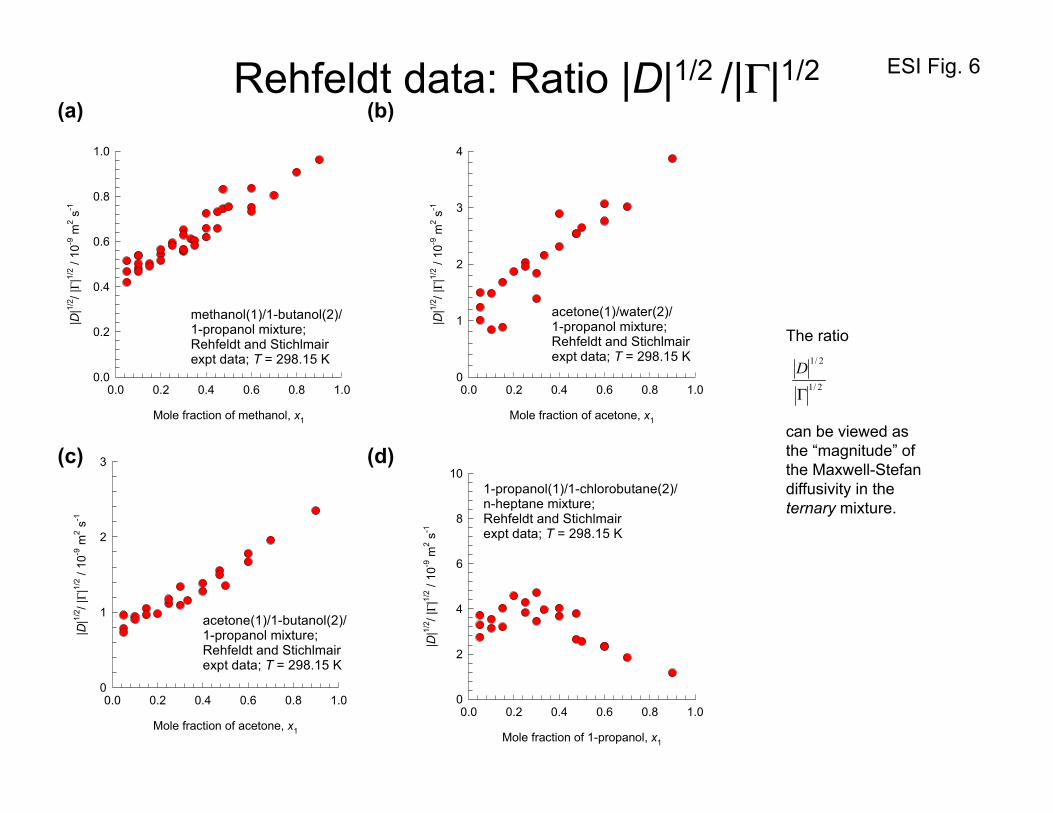
ESI Fig. 6

1-propanol(1)/1-chlorobutane(2)/n-heptane mixture; Rehfeldt and Stichlmair expt data; T = 298.15 K

Mole fraction of 1-propanol, x1

0.0 0.2 0.4 0.6 0.8 1.0

|D|1/

2 / |Γ|

1/2 /

10-9

m2 s

-1

0

2

4

6

8

10

acetone(1)/1-butanol(2)/1-propanol mixture; Rehfeldt and Stichlmair expt data; T = 298.15 K

Mole fraction of acetone, x1

0.0 0.2 0.4 0.6 0.8 1.0

|D|1/

2 / |Γ|

1/2 /

10-9

m2 s

-1

0

1

2

3

Mole fraction of acetone, x1

0.0 0.2 0.4 0.6 0.8 1.0

|D|1/

2 / |Γ|

1/2 /

10-9

m2 s

-1

0

1

2

3

4

acetone(1)/water(2)/1-propanol mixture; Rehfeldt and Stichlmair expt data; T = 298.15 K

Mole fraction of methanol, x1

0.0 0.2 0.4 0.6 0.8 1.0

|D|1/

2 / |Γ |

1/2 /

10-9

m2 s

-1

0.0

0.2

0.4

0.6

0.8

1.0

methanol(1)/1-butanol(2)/1-propanol mixture; Rehfeldt and Stichlmair expt data; T = 298.15 K

Rehfeldt data: Ratio |D|1/2 /|Γ|1/2(a) (b)

(c) (d)

The ratio

can be viewed as the “magnitude” of the Maxwell-Stefan diffusivity in the ternary mixture.

2/1

2/1

Γ

D

ESI Fig. 7Ziebold data: Ratio |D|1/2 /|Γ|1/2

atom fraction Cu, x1

0.0 0.2 0.4 0.6 0.8 1.0

|D|1/

2 / |Γ|

1/2 /

10-1

4 m2 s

-1

0.1

1

10Cu(1)/Ag(2)/Au(3);T = 998 K

ESI Fig. 8

H2/N2/CO2 gas mixture diffusion

78 mL glassbulb

Capillary tube; L = 86 mm; d = 2 mm;

T = 308.3 K

Initial Compositions:H2 = 0.0N2 = 0.50086CO2 = 0.49914

Initial Compositions:H2 = 0.50121N2 = 0.49879CO2 = 0.0

Bulb A Bulb B

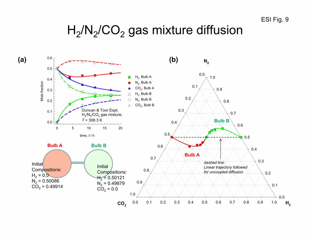
ESI Fig. 9

H20.0 0.1 0.2 0.3 0.4 0.5 0.6 0.7 0.8 0.9 1.0

N2

0.0

0.1

0.2

0.3

0.4

0.5

0.6

0.7

0.8

0.9

1.0

CO2

0.0

0.1

0.2

0.3

0.4

0.5

0.6

0.7

0.8

0.9

1.0

time, t / h

0 5 10 15 20

Mol

e fra

ctio

n

0.0

0.1

0.2

0.3

0.4

0.5

0.6

H2, Bulb AN2, Bulb ACO2, Bulb AH2, Bulb BN2, Bulb BCO2, Bulb B

Duncan & Toor Expt;H2/N2/CO2 gas mixture;T = 308.3 K

H2/N2/CO2 gas mixture diffusion

Bulb A

Bulb B

(a) (b)

Initial Compositions:H2 = 0.0N2 = 0.50086CO2 = 0.49914

Bulb A Bulb B

Initial Compositions:H2 = 0.50121N2 = 0.49879CO2 = 0.0

dashed line:Linear trajectory followed for uncoupled diffusion

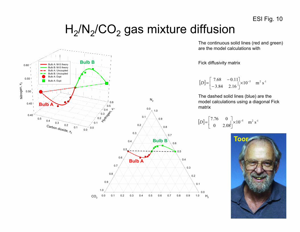
ESI Fig. 10

H20.0 0.1 0.2 0.3 0.4 0.5 0.6 0.7 0.8 0.9 1.0

N2

0.0

0.1

0.2

0.3

0.4

0.5

0.6

0.7

0.8

0.9

1.0

CO2

0.0

0.1

0.2

0.3

0.4

0.5

0.6

0.7

0.8

0.9

1.0

0.40

0.45

0.50

0.55

0.60

0.0

0.1

0.20.3

0.40.5

0.6

0.00.1

0.20.3

0.40.5

Nitr

ogen

, x2

Hydro

gen,

x 1

Carbon dioxide, x3

Bulb A: M-S theoryBulb B: M-S theoryBulb A: UncoupledBulb B: UncoupledBulb A: Expt

Bulb A: Expt

Bulb A

Bulb B

Bulb A

Bulb B

H2/N2/CO2 gas mixture diffusion

Fick diffusivity matrix

[ ] 1-25 s m1016.284.3

11.068.7 −×

−

−=D

The continuous solid lines (red and green) are the model calculations with

The dashed solid lines (blue) are the model calculations using a diagonal Fick matrix

[ ] 1-25 s m1008.20

076.7 −×

=D

Toor

ESI Fig. 11

time, t / h

0 5 10 15 20

Mol

e fra

ctio

n

0.40

0.45

0.50

0.55

0.60

N2, Bulb AN2, Bulb BN2, M-S Bulb AN2, M-S Bulb BUncoupled, Bulb AUncoupled, Bulb B

Duncan & Toor Expt;H2/N2/CO2 gas mixture;T = 308.3 K

time, t / h

0 5 10 15 20

Mol

e fra

ctio

n

0.0

0.1

0.2

0.3

0.4

0.5

H2, Bulb ACO2, Bulb AH2, Bulb BCO2, Bulb BH2, M-S Bulb ACO2, M-S Bulb AH2, M-S Bulb BCO2, M-S Bulb B

Duncan & Toor Expt;H2/N2/CO2 gas mixture;T = 308.3 K

H2/N2/CO2 gas mixture diffusion

t = t1

1-2523

1-2513

-12512

s m1068.1

s m108.6

s m1033.8

−

−

−

×=

×=

×=

Ð

Ð

Ð

Fick diffusivity matrix

M-S diffusivities

[ ] 1-25 s m10

16.284.3

11.068.7 −×

−

−=D

Transient over(under)shoots are captured by Maxwell-Stefan model

23

2332

13

13313

23

3223

12

12212

13

3113

12

21121 ;

Ðc

NxNx

Ðc

NxNx

dz

dx

Ðc

NxNx

Ðc

NxNx

dz

dx

Ðc

NxNx

Ðc

NxNx

dz

dx

tt

tt

tt

−+−=−

−+−=−

−+−=−

ESI Fig. 12

Hydrogen driving force (x1A-x1B)

-0.6 -0.4 -0.2 0.0 0.2

Dim

ensi

onle

ss h

ydro

gen

flux

(N1 δ

/ct)/

106

-40

-30

-20

-10

0

Duncan & Toor Expt;H2/N2/CO2 gas mixture;T = 308.3 K

Carbon dioxide driving force (x3A-x3B)

0.0 0.1 0.2 0.3 0.4 0.5 0.6Dim

ensi

onle

ss c

arbo

n di

oxid

e flu

x (N

3 δ

/ct)/

106

0

5

10

15

20

Duncan & Toor Expt;H2/N2/CO2 gas mixture;T = 308.3 K

(a) Hydrogen flux vs driving force

(c) Carbon dioxide flux vs driving force

(b) Nitrogen flux vs driving force

Nitrogen driving force (x2A-x2B)

-0.20 -0.15 -0.10 -0.05 0.00

Dim

ensi

onle

ss n

troge

n flu

x (N

2 δ /c

t)/10

6

-5

0

5

10

15

20

Duncan & Toor Expt;H2/N2/CO2 gas mixture;T = 308.3 K

t > 6 h: normal diffusion

Osmotic diffusion at t = 0 h

DiffusionBarrier at t1 ≈ 6 h

ESI Fig. 13

Osmotic diffusion

DiffusionBarrier uphill

diffusion

iJ

(a) Binary diffusion (b) Ternary diffusion

00dz

dxi−

Fick’s law with constant diffusivity

dz

dxi- Force Driving =

ESI Fig. 14

H2/N2/CO2 gas mixture diffusion

H20.0 0.1 0.2 0.3 0.4 0.5 0.6 0.7 0.8 0.9 1.0

N2

0.0

0.1

0.2

0.3

0.4

0.5

0.6

0.7

0.8

0.9

1.0

CO2

0.0

0.1

0.2

0.3

0.4

0.5

0.6

0.7

0.8

0.9

1.0

fast eigenvector slow

eigenvector

fast eigenvector

sloweigenvector

ESI Fig. 15

CH40.0 0.1 0.2 0.3 0.4 0.5 0.6 0.7 0.8 0.9 1.0

Ar

0.0

0.1

0.2

0.3

0.4

0.5

0.6

0.7

0.8

0.9

1.0

H2

0.0

0.1

0.2

0.3

0.4

0.5

0.6

0.7

0.8

0.9

1.0

BOTTOM

TOP

dashed line:Linear trajectory followed for uncoupled diffusion

CH4/Ar/H2 gas mixture diffusion in Loschmidt tube

Fick diffusivity matrix

The continuous solid lines (red and green) are the model calculations with

The dashed solid lines (blue) are the model calculations using a diagonal Fick matrix

[ ] 1-25 s m103.664.3

83.144.4 −×

−

=D

[ ] 1-25 s m1063.20

011.8 −×

=D

0.40

0.45

0.50

0.55

0.60

0.0

0.1

0.20.3

0.40.5

0.6

0.00.1

0.20.3

0.40.5

argo

n, x

2

metha

ne, x 1

hydrogen, x3

BOTTOM M-S theoryTOP: M-S theoryBOTTOM Expt data

TOP Expt data

Initial Compositions:CH4 = 0.0Ar = 0.509H2 = 0.491

Initial Compositions:CH4 = 0.515Ar = 0.485H2 = 0

ESI Fig. 16

CH40.0 0.1 0.2 0.3 0.4 0.5 0.6 0.7 0.8 0.9 1.0

Ar

0.0

0.1

0.2

0.3

0.4

0.5

0.6

0.7

0.8

0.9

1.0

H2

0.0

0.1

0.2

0.3

0.4

0.5

0.6

0.7

0.8

0.9

1.0

CH4/Ar/H2 gas mixture diffusion

BOTTOM

TOP

time, t / h

0.0 0.2 0.4 0.6 0.8 1.0 1.2

Mol

e fra

ctio

n

0.0

0.1

0.2

0.3

0.4

0.5

0.6

CH4, BottomAr, BottomH2, BottomCH4, TopAr, TopH2, Top

Arnold & Toor Expt;CH4/Ar/H2 gas mixture;T = 307 K

Initial Compositions:CH4 = 0.0Ar = 0.509H2 = 0.491

Initial Compositions:CH4 = 0.515Ar = 0.485H2 = 0

(a) (b)

dashed line:Linear trajectory followed for uncoupled diffusion

ESI Fig. 17

time, t / h

0.0 0.5 1.0 1.5 2.0

Mol

e fra

ctio

n

0.0

0.1

0.2

0.3

0.4

0.5CH4, BottomH2, BottomCH4, TopH2, TopCH4, M-S BottomH2, M-S BottomCH4, M-S TopH2, M-S TopArnold & Toor Expt;

CH4/Ar/H2 gas mixture;T = 307 K

Transient approaches to Equilibrium

Transient over(under)shoots are captured by taking account of coupling effects

Coupled:

[ ] 1-25 s m103.664.3

83.144.4 −×

−

=D

time, t / h

0.0 0.5 1.0 1.5 2.0

Mol

e fra

ctio

n

0.40

0.45

0.50

0.55

Ar, Coupled, BottomAr, Coupled, TopAr, Uncoupled, BottomAr, Uncoupled, TopAr, BottomAr, Top

Arnold & Toor Expt;CH4/Ar/H2 gas mixture;T = 307 K

[ ] 1-25 s m1063.20

011.8 −×

=D

Uncoupled:

ESI Fig. 18

0.16

0.18

0.20

0.22

0.24

0.0

0.2

0.4

0.6

0.8

0.00.2

0.40.6

Oxy

gen,

x1

Nitroge

n, x 2

Helium, x3

Maxwell-StefanUncoupled

Heliox

Air

O2/N2/He gas mixture diffusion

Heliox

0.8 He0.2 O2

Air in patient

0.8 N20.2 O2

Left Right

z = 0

Heliox

0.8 He0.2 O2

ESI Fig. 19

O2/N2/He gas mixture diffusionHeliox

0.8 He0.2 O2

Air in patient

0.8 N20.2 O2

Left Right

z = 0

z = -0.5

time, t / h

0 2 4 6 8 10

Mol

e fra

ctio

n O

2

0.19

0.20

0.21

0.22

0.23Maxwell-Stefanuncoupled diffusion

O2/N2/He gas mixture;T = 298 K

ESI Fig. 20Breaking azeotropes by partial condensation

2-propanolwater

nitrogen

Water flux

condensate

2-propanol flux

ESI Fig. 21

Mole fraction of n-hexane, x1

0.0 0.2 0.4 0.6 0.8 1.0

Tem

pera

ture

, T /

K

270

275

280

285

290

295

n-hexane (1) - nitrobenzene (2);x1c= 0.578;Tc = 292.56 K

UCST =292.56 K

Mole fraction of methanol, x1

0.0 0.2 0.4 0.6 0.8 1.0

Tem

pera

ture

, T /

K

260

270

280

290

300

310

320

Methanol (1) - n-hexane (2)

UCST and LCST(a) methanol(1)/n-hexane(2)

UCST

Mole fraction of triethylamine, x1

0.0 0.1 0.2 0.3 0.4

Tem

pera

ture

, T /

K

291

292

293

294

295

296

297triethylamine (1) -water (2)

LCST

0

;0

>>Γ

D

0

;0

==Γ

D

0

;0

<<Γ

D

unstable

Homogeneous phase

(b) triethylamine(1)/water(2)

(c) n-hexane(1)/nitrobenzene(2)

ESI Fig. 22

Mole fraction of methanol, x1

0.0 0.2 0.4 0.6 0.8 1.0Te

mpe

ratu

re, T

/ K

260

270

280

290

300

310

spinodalbinodal

Methanol (1) - n-hexane (2)

UCST

Mole fraction of methanol, x1

0.0 0.2 0.4 0.6 0.8 1.0

Sec

ond

deriv

ativ

e, (d

2 G/d

x2 )/RT

-2

-1

0

1

320 K310 K300 K290 K280 K270 K260 KSpinodal

Methanol (1) - n-hexane (2)

Spin

odal

deco

mpo

sitio

n

Binodal and spinodal(c)

(d)

These intersection points define the binodal curve

Mole fraction of methanol, x1

0.0 0.2 0.4 0.6 0.8 1.0

Free

Ene

rgy,

G /

RT

-0.2

-0.1

0.0

0.1

320 K310 K300 K290 K280 K270 K260 KBinodal

Methanol (1) - n-hexane (2)

Mole fraction of methanol, x1

0.0 0.2 0.4 0.6 0.8 1.0

Firs

t der

ivat

ive,

(dG

/dx)

/RT

-1.0

-0.5

0.0

0.5

1.0

320 K310 K300 K290 K280 K270 K260 KBinodal

Methanol (1) - n-hexane (2)

(b)These intersection points define the spinodal curve

(a)

0

1

=∂∂x

G

021

2

=∂∂

x

G

ESI Fig. 23

Mole fraction of methanol, x1

0.0 0.2 0.4 0.6 0.8 1.0

Ther

mod

ynam

ic c

orre

ctio

n fa

ctor

, Γ 1

0.01

0.1

1

313.15 K310.65 K307.75 K305.65 K303.15 K273.15 K

Methanol (1) - n-hexane (2)

Methanol/n-hexane mixture diffusion

(a) (b) Mole fraction of methanol, x1

0.0 0.2 0.4 0.6 0.8 1.0

Fick

diff

usiv

ity, D

/ 10

-8 m

2 s-1

0.00

0.05

0.10

0.15

0.20

0.25

0.30 303.15 K305.65 K307.75 K310.65 K313.15 K

Methanol (1) - n-hexane (2);Clark & Rowley

Mole fraction of methanol, x1

0.0 0.2 0.4 0.6 0.8 1.0

Fick

diff

usiv

ity, D

/ 10

-8 m

2 s-1

0.01

0.1

1303.15 K305.65 K307.75 K310.65 K313.15 K

Methanol (1) - n-hexane (2)

Mole fraction of methanol, x1

0.0 0.2 0.4 0.6 0.8 1.0

Ther

mod

ynam

ic c

orre

ctio

n fa

ctor

, Γ

0.0

0.2

0.4

0.6

0.8

1.0

313.15 K310.65 K307.75 K305.65 K303.15 K

Methanol (1) - n-hexane (2)

Demixing region

ESI Fig. 24

Mole fraction of methanol, x1

0.0 0.2 0.4 0.6 0.8 1.0D

iffus

ivity

, D12

, Ð

12 /

10-8

m2 s

-1

0.0

0.1

0.2

0.3

0.4

0.5Fick D12, exptFick D12, MDM-S Ð12, MD

Methanol (1) - n-hexane (2);305.65 K

Mole fraction of methanol, x1

0.0 0.2 0.4 0.6 0.8 1.0

Diff

usiv

ity, D

12 ,

Ð12

/ 10

-8 m

2 s-1

0.0

0.1

0.2

0.3

0.4

0.5Fick D12, ExptFick D12, MD M-S Ð12, MD

Methanol (1) - n-hexane (2);307.75 K

Methanol/n-hexane mixture diffusion

Mole fraction of methanol, x1

0.0 0.2 0.4 0.6 0.8 1.0

Diff

usiv

ity, D

12 ,

Ð12

/ 10

-8 m

2 s-1

0.0

0.1

0.2

0.3

0.4

0.5Fick D12, ExptFick D12, MD M-S Ð12, MD

Methanol (1) - n-hexane (2);310.65 K

Mole fraction of methanol, x1

0.0 0.2 0.4 0.6 0.8 1.0

Diff

usiv

ity, D

12 ,

Ð12

/ 10

-8 m

2 s-1

0.0

0.1

0.2

0.3

0.4

0.5Fick D12, ExptFick D12, MD M-S Ð12, MD

Methanol (1) - n-hexane (2);303.15 K

Mole fraction of methanol, x1

0.0 0.2 0.4 0.6 0.8 1.0D

iffus

ivity

, D12

, Ð

12 /

10-8

m2 s

-10.0

0.1

0.2

0.3

0.4

0.5 Fick D12, ExptFick D12, MD M-S Ð12, MD

Methanol (1) - n-hexane (2);313.15 K

(a) (b)

(c) (d) (e)

ESI Fig. 25Methanol/n-hexane mixture diffusion

Mole fraction of methanol, x1

0.0 0.2 0.4 0.6 0.8 1.0

Diff

usiv

ity /

10-8

m2 s

-1

0.001

0.01

0.1

1

Vignes InterpolationM-S Ð12

Fick D12

Onsager L12

Methanol (1) - n-hexane (2); 313.15 K

ESI Fig. 26Triethylamine/water mixture diffusion

Mole fraction of triethanolamine, x1

0.01 0.1 1

Ther

mod

ynam

ic c

orre

ctio

n fa

ctor

, Γ

0.001

0.01

0.1

1

T = 277.15 KT = 283.15 KT = 291.15 Kcritical composition

triethylamine(1) - water (2)

(a) (b)

Temperature, T

270 275 280 285 290

Fick

diff

usiv

ity, D

12 /

10-1

1 m2 s

-1

0.1

1

10Haase dataLCST = 291.5 K

Haase & Siry expt data;triethylamine(1) - water (2);x1 = 0.073

ESI Fig. 27Tri-ethylamine/water mixture diffusion

Mole fraction of triethylamine, x1

0.0 0.1 0.2 0.3 0.4

Fick

diff

usiv

ity, D

12 /

10-1

0 m2 s

-1

0

1

2

3

4

5

6293.15 K292.15 K

Vitagliano expt data;triethylamine(1) - water (2)

(b)

(a)

Spinodalcompositions

Mole fraction of triethylamine, x1

0.0 0.1 0.2 0.3 0.4

Tem

pera

ture

, T /

K

291

292

293

294

295

296

297triethylamine (1) -water (2)

LCST

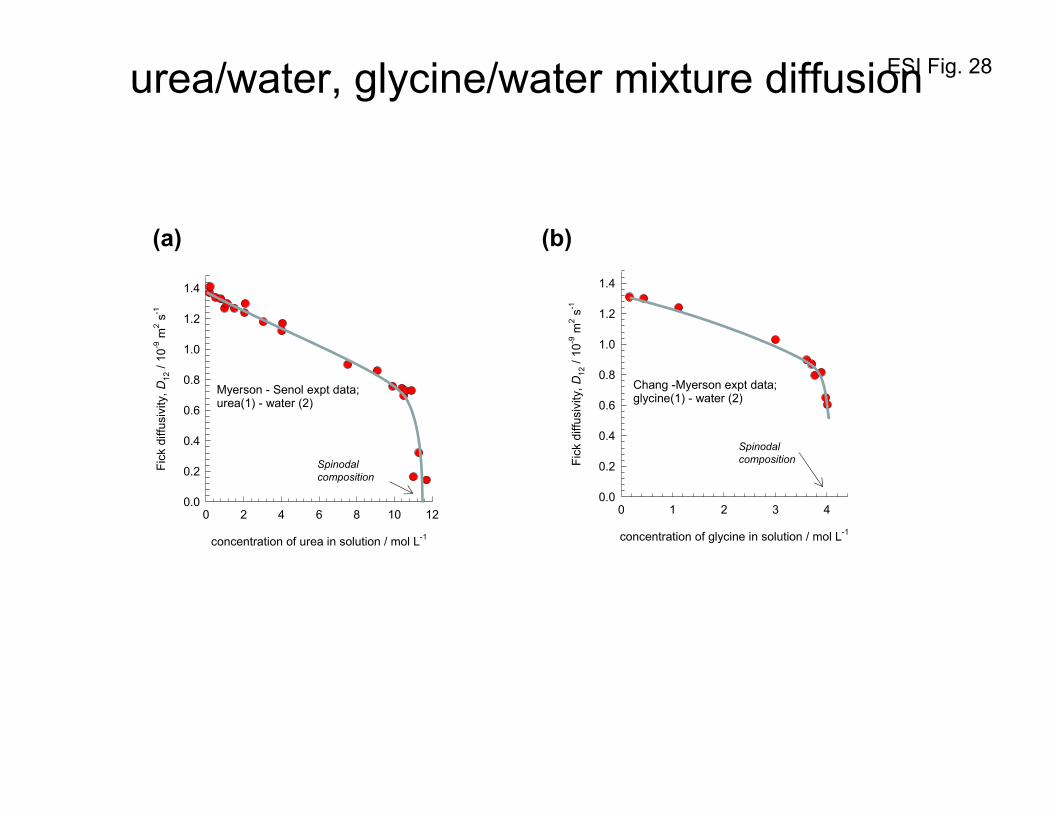
ESI Fig. 28urea/water, glycine/water mixture diffusion

concentration of urea in solution / mol L-1

0 2 4 6 8 10 12

Fick

diff

usiv

ity, D

12 /

10-9

m2 s

-1

0.0

0.2

0.4

0.6

0.8

1.0

1.2

1.4

Myerson - Senol expt data;urea(1) - water (2)

Spinodalcomposition

(a) (b)

concentration of glycine in solution / mol L-1

0 1 2 3 4

Fick

diff

usiv

ity, D

12 /

10-9

m2 s

-1

0.0

0.2

0.4

0.6

0.8

1.0

1.2

1.4

Chang -Myerson expt data;glycine(1) - water (2)

Spinodalcomposition

ESI Fig. 29

Mole fraction of n-hexane, x1

0.0 0.2 0.4 0.6 0.8 1.0

Tem

pera

ture

, T /

K

270

275

280

285

290

295

n-hexane (1) - nitrobenzene (2);x1c= 0.578;Tc = 292.56 K

n-hexane(1)-nitrobenzene(2) diffusion

UCST =292.56 K

(T-Tc) / K

0 5 10 15

Fick

Diff

usiv

ity /

10-1

0 m2 s

-1

0.0

0.5

1.0

1.5

2.0

2.5

3.0 Matos-Lopes expt dataHaase & Siry expt dataWu et al. expt data

n-hexane(1)/nitrobenzene(2);x1c= 0.578;Tc = 292.56 K

ESI Fig. 30Nucleation and Growth

Top

Bottom

Concentration of component 2

Component 2Event 1 Event 2 Event 3 Event 4

ESI Fig. 31Spinodal Decomposition

Top

Bottom

Concentration of component 2

Component 2Event 1 Event 2 Event 3 Event 4

ESI Fig. 32Ternary Liquid/Liquid System

Plait point

Spinodalcurve

Component 3

Component 1

Component 2

Meta-stable region

Two liquid phases

Homogeneous region

M

eq

eqA

B

0

;0

2221

1211

2221

1211

>

>ΓΓΓΓ

DD

DD

0

;0

2221

1211

2221

1211

<

<ΓΓΓΓ

DD

DD

0

;0

2221

1211

2221

1211

=

=ΓΓΓΓ

DD

DD

ESI Fig. 33

Glycerol0.0 0.1 0.2 0.3 0.4 0.5 0.6 0.7 0.8 0.9 1.0

Water

0.0

0.1

0.2

0.3

0.4

0.5

0.6

0.7

0.8

0.9

1.0

Acetone

0.0

0.1

0.2

0.3

0.4

0.5

0.6

0.7

0.8

0.9

1.0

glycerol(1)/acetone(2)/water(3) mixture;T = 298 K

Fick diffusivities in Glycerol/Acetone/Water

[ ]

044.0

;213.0148.0

127.0294.0

=

=

D

D

[ ]

=Γ

444.0478.0

73.083.1

0

2221

1211 =DD

DD

Plait point

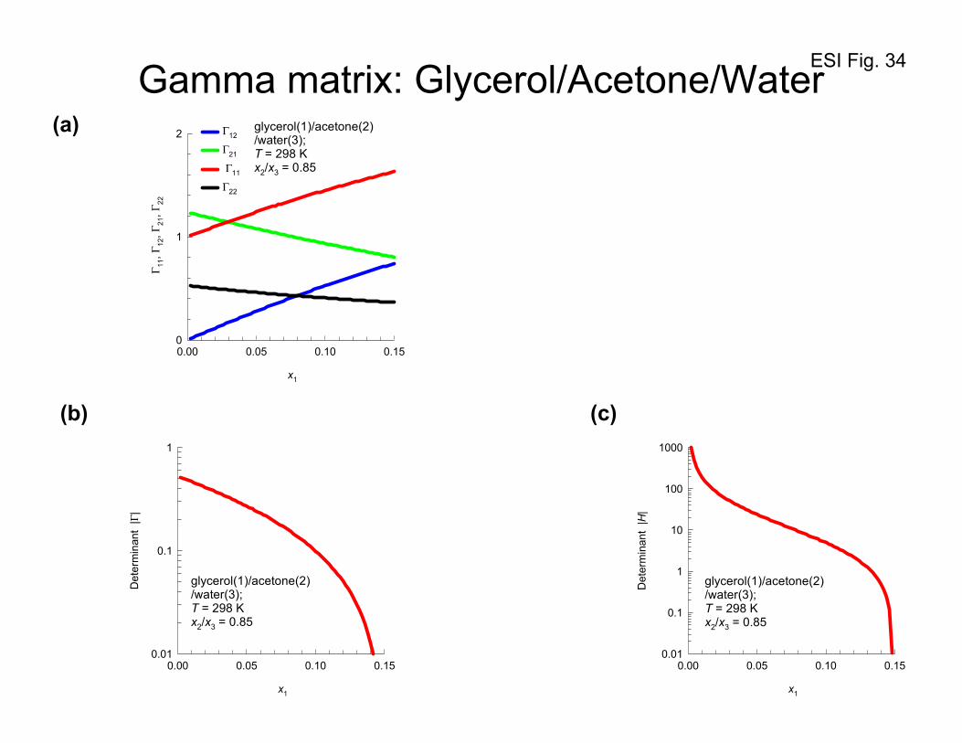
ESI Fig. 34

x1

0.00 0.05 0.10 0.15

Γ11

, Γ12

, Γ21

, Γ22

0

1

2 Γ12

Γ21

Γ11

Γ22

glycerol(1)/acetone(2)/water(3);T = 298 Kx2/x3 = 0.85

Gamma matrix: Glycerol/Acetone/Water

(b) (c)

(a)

x1

0.00 0.05 0.10 0.15

Det

erm

inan

t |Γ

|

0.01

0.1

1

glycerol(1)/acetone(2)/water(3);T = 298 Kx2/x3 = 0.85

x1

0.00 0.05 0.10 0.15

Det

erm

inan

t |H

|0.01

0.1

1

10

100

1000

glycerol(1)/acetone(2)/water(3);T = 298 Kx2/x3 = 0.85

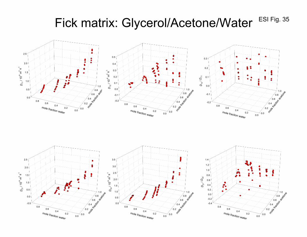
ESI Fig. 35

0.0

0.5

1.0

1.5

2.0

2.5

3.0

3.5

0.0

0.2

0.4

0.6

0.81.0

0.00.2

0.40.6

0.8

D22

/ 10

-9 m

2 s-1

mole fr

actio

n ac

eton

e

mole fraction water

Col 78 vs Col 79 vs Col 83

-0.4

-0.2

0.0

0.2

0.4

0.6

0.8

1.0

1.2

1.4

0.0

0.2

0.4

0.6

0.81.0

0.00.2

0.40.6

0.8

D21

/ D

22

mole fr

actio

n ace

tone

mole fraction water

-0.5

0.0

0.5

1.0

1.5

2.0

2.5

0.0

0.2

0.4

0.6

0.81.0

0.00.2

0.40.6

0.8

D21

/ 10

-9 m

2 s-1

mole fr

actio

n ace

tone

mole fraction water

Fick matrix: Glycerol/Acetone/Water

0.0

0.5

1.0

1.5

2.0

2.5

0.0

0.2

0.4

0.6

0.81.0

0.00.2

0.40.6

0.8

D11

/ 10

-9 m

2 s-1

mole fr

actio

n ac

eton

emole fraction water

-0.2

-0.1

0.0

0.1

0.2

0.3

0.4

0.5

0.0

0.2

0.4

0.6

0.81.0

0.00.2

0.40.6

0.8

D12

/ 10

-9 m

2 s-1

mole fr

actio

n ace

tone

mole fraction water

Col 78 vs Col 79 vs Col 82

-0.2

-0.1

0.0

0.1

0.2

0.3

0.0

0.2

0.4

0.6

0.81.0

0.00.2

0.40.6

0.8

D12

/ D

11

mole fr

actio

n ace

tone

mole fraction water

ESI Fig. 36

Glycerol0.0 0.1 0.2 0.3 0.4 0.5 0.6 0.7 0.8 0.9 1.0

Water

0.0

0.1

0.2

0.3

0.4

0.5

0.6

0.7

0.8

0.9

1.0

Acetone

0.0

0.1

0.2

0.3

0.4

0.5

0.6

0.7

0.8

0.9

1.0

glycerol(1)/acetone(2)/water(3) mixture;T = 298 K

0

2

4

6

8

0.00.2

0.40.6

0.81.0

0.00 0.05 0.10 0.150.20

Det

erm

inan

t |D

| / 1

0-18 m

4 s-2

mole fraction acetone

mole fraction glycerol

Plait point

glycerol/acetone/watermixture;T = 298 K

Glycerol/Acetone/Water Mixture Diffusion

Plait point

x10= 0.1467x20= 0.4163x30= 0.4360

Col 78 vs Col 79 vs Col 83

0.0

0.2

0.4

0.6

0.8

1.0

1.2

1.4

1.6

0.00 0.05 0.10 0.15 0.20

0.00.20.40.60.81.0

Det

erm

inan

t |Γ |

mole fraction glycerol

mole fraction acetone

Plait point

glycerol/acetone/watermixture;T = 298 K

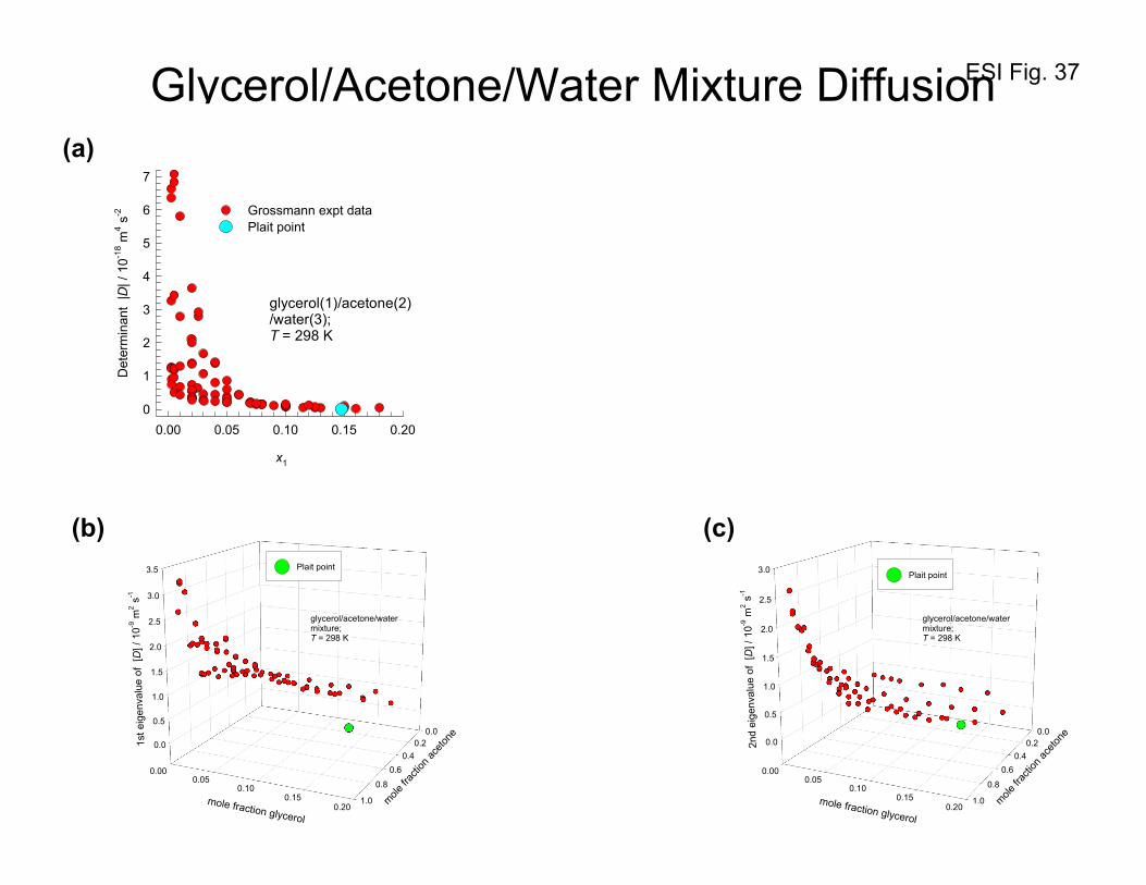
ESI Fig. 37Glycerol/Acetone/Water Mixture Diffusion

0.0

0.5

1.0

1.5

2.0

2.5

3.0

0.00.2

0.40.6

0.8

1.0

0.000.05

0.100.15

0.20

2nd

eige

nval

ue o

f [D

] / 1

0-9 m

2 s-1

mole fra

ction

aceto

ne

mole fraction glycerol

Plait point

glycerol/acetone/watermixture;T = 298 K

0.0

0.5

1.0

1.5

2.0

2.5

3.0

3.5

0.00.2

0.40.6

0.8

1.0

0.000.05

0.100.15

0.20

1st e

igen

valu

e of

[D

] / 1

0-9 m

2 s-1

mole fra

ction

aceto

ne

mole fraction glycerol

Plait point

glycerol/acetone/watermixture;T = 298 K

(b) (c)

(a)

x1

0.00 0.05 0.10 0.15 0.20

Det

erm

inan

t |D

| / 1

0-18 m

4 s-2

0

1

2

3

4

5

6

7

Grossmann expt dataPlait point

glycerol(1)/acetone(2)/water(3);T = 298 K

ESI Fig. 38Strength of Coupling vs Determinant |D|

(a) (b)

Determinant |D| / 10-18 m4 s-2

0.01 0.1 1 10

D12

/D11

, and

D21

/D22

0.001

0.01

0.1

1

D12/D11

D21/D22

glycerol(1)/acetone(2)/water(3);T = 298 K

Determinant |D| / 10-18 m4 s-2

0.01 0.1 1 10

D12

/D11

, and

Γ12

/Γ11

0.01

0.1

1

D12/D11

Γ12/Γ11

glycerol(1)/acetone(2)/water(3); T = 298 K

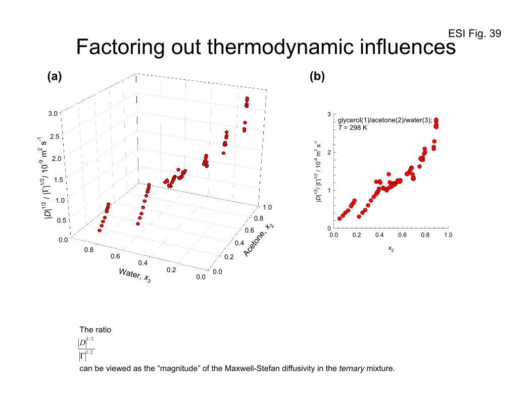
ESI Fig. 39

0.0

0.5

1.0

1.5

2.0

2.5

3.0

0.0

0.2

0.4

0.6

0.81.0

0.00.2

0.40.6

0.8

|D|1/

2 / |Γ

|1/2 / 1

0-9 m

2 s-1

Aceto

ne, x 2

Water, x3

x2

0.0 0.2 0.4 0.6 0.8 1.0

|D|1/

2 / |Γ |

1/2 /

10-9

m2 s

-1

0

1

2

3glycerol(1)/acetone(2)/water(3);T = 298 K

Factoring out thermodynamic influences

The ratio

can be viewed as the “magnitude” of the Maxwell-Stefan diffusivity in the ternary mixture.

2/1

2/1

Γ

D

(a) (b)

ESI Fig. 40

Chloroform0.0 0.1 0.2 0.3 0.4 0.5 0.6 0.7 0.8 0.9 1.0

Acetic Acid

0.0

0.1

0.2

0.3

0.4

0.5

0.6

0.7

0.8

0.9

1.0

Water

0.0

0.1

0.2

0.3

0.4

0.5

0.6

0.7

0.8

0.9

1.0

Water/Chloroform/Acetic Acid Diffusion

Plait point

[ ] 21.1;259.1073.0

13.097.0=

= DD

[ ] 854.0;135.1172.0

194.0782.0=

= DD

[ ] 696.0;105.1196.0

236.0672.0=

= DD

[ ] 395.0;983.0295.0

321.04982.0=

= DD

[ ] 164.0;939.0344.0

368.0309.0=

= DD

[ ] 0;161.037.0

4.092.0=

= DD

Meta-stable region

Homogeneous region

0

;0

2221

1211

2221

1211

>

>ΓΓΓΓ

DD

DD

0

;0

2221

1211

2221

1211

<

<ΓΓΓΓ

DD

DD

0

;0

2221

1211

2221

1211

=

=ΓΓΓΓ

DD

DD

Phase-splitting region

ESI Fig. 41

Chloroform0.0 0.1 0.2 0.3 0.4 0.5 0.6 0.7 0.8 0.9 1.0

Acetic Acid

0.0

0.1

0.2

0.3

0.4

0.5

0.6

0.7

0.8

0.9

1.0

Water

0.0

0.1

0.2

0.3

0.4

0.5

0.6

0.7

0.8

0.9

1.0

Water/Chloroform/Acetic Acid Diffusion

[ ] 137.0;544.0181.0

461.0406.0=

= DD

[ ] 207.0;699.0117.0

540.0386.0=

= DD

[ ] 336.0;728.0185.0

403.0564.0=

= DD

[ ] 450.0;811.0138.0

451.0632.0=

= DD

[ ] 474.0;753.0107.0

394.0685.0=

= DD

Plait point

Water(1)/Chloroform(2)/Acetic acid(3)Mixture;298.15 K

ESI Fig. 42

(1-x3)

0.0 0.1 0.2 0.3 0.4 0.5 0.6 0.7

Det

erm

inan

t |Γ

|0.0

0.2

0.4

0.6

0.8

1.0

1.2

Vitagliano exptBuzatu exptPlait point

water/chloroform/acetic acid;T = 298 K

(1-x3)

0.0 0.1 0.2 0.3 0.4 0.5 0.6 0.7

Det

erm

inan

t |D

| / 1

0-18 m

4 s-2

0.0

0.2

0.4

0.6

0.8

1.0

1.2

1.4

Vitagliano expt dataBuzatu expt dataPlait point

water/chloroform/acetic acid;T = 298 K

Strength of Coupling vs Determinant of [D]

Determinant of [D] / 10-18 m4 s-2

0.0 0.2 0.4 0.6 0.8 1.0 1.2

D12

/D11

, and

D21

/D22

0.0

0.5

1.0

1.5 D12/D11

D21/D22

water/chloroform/acetic acid;T = 298 K

Determinant of [Γ]

0.0 0.2 0.4 0.6 0.8 1.0 1.2

Γ 12/Γ

11, a

nd Γ

21/Γ

22

0.0

0.5

1.0

1.5

Γ12/Γ11

Γ21/Γ22

water/chloroform/acetic acid;T = 298 K

(a) (b)(c)

(d) (e)(1-x3)

0.0 0.1 0.2 0.3 0.4 0.5 0.6 0.7

|D|1/

2 / |Γ|

1/2 /

10-9

m2 s

-1

0.0

0.2

0.4

0.6

0.8

1.0

1.2

1.4

Vitagliano expt dataBuzatu expt data

water/chloroform/acetic acid;T = 298 K

The ratio

can be viewed as the “magnitude” of the Maxwell-Stefan diffusivity in the ternary mixture.

2/1

2/1

Γ

D

ESI Fig. 43

(T-Tc) / K

01234567

Det

erm

inan

t |D

| / 1

0-18 m

4 s-2

0

2

4

6

8

10

12

14

water(1)/2-propanol(2)/cyclohexane(3);plait point composition:x1=0.367; x2=0.389; x3=0.244;

Water/2-propanol/cyclohexane mixture diffusion

mole fraction of water, x1

0.2 0.3 0.4 0.5 0.6

mol

e fra

ctio

n of

2-p

ropa

nol,

x 2

0.34

0.36

0.38

0.40

293.15 K303.15 K323.15 KPlait point

water(1)/2-propanol(2)/cyclohexane(3);plait point:x1=0.367; x2=0.389; x3=0.244;

(a)

(b)

[ ] 082.13;984.112.2

064.1071.1=

−−

= DD

[ ] 847.4;064.1997.0

547.0467.0=

−−

= DD

[ ] 921.0;

571.0566.0

328.0309.0=

−−

= DD

[ ] 466.0;439.0440.0

267.0257.0=

−−

= DD

[ ] 359.0;510.0559.0

323.0347.0=

−−

= DD

Units: 10-10 m2 s-1

Units: 10-18 m4 s-2

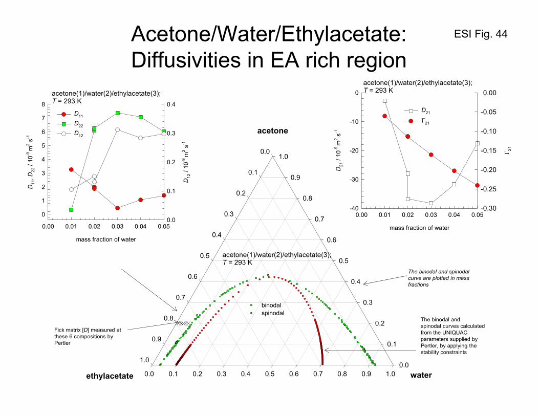
ESI Fig. 44

water0.0 0.1 0.2 0.3 0.4 0.5 0.6 0.7 0.8 0.9 1.0

acetone

0.0

0.1

0.2

0.3

0.4

0.5

0.6

0.7

0.8

0.9

1.0

ethylacetate

0.0

0.1

0.2

0.3

0.4

0.5

0.6

0.7

0.8

0.9

1.0

binodalspinodal

acetone(1)/water(2)/ethylacetate(3);T = 293 K

Fick matrix [D] measured at these 6 compositions by Pertler

The binodal and spinodalcurve are plotted in mass fractions

The binodal andspinodal curves calculated from the UNIQUAC parameters supplied by Pertler, by applying the stability constraints

mass fraction of water

0.00 0.01 0.02 0.03 0.04 0.05

D11

, D22

/ 10

-9 m

2 s-1

0

1

2

3

4

5

6

7

8

D12

/ 10

-9 m

2 s-1

0.0

0.1

0.2

0.3

0.4D11

D22

D12

acetone(1)/water(2)/ethylacetate(3);T = 293 K

mass fraction of water

0.00 0.01 0.02 0.03 0.04 0.05

D21

/ 10

-9 m

2 s-1

-40

-30

-20

-10

0

Γ 21

-0.30

-0.25

-0.20

-0.15

-0.10

-0.05

0.00

D21

Γ21

acetone(1)/water(2)/ethylacetate(3);T = 293 K

Acetone/Water/Ethylacetate:Diffusivities in EA rich region

ESI Fig. 45

water0.0 0.1 0.2 0.3 0.4 0.5 0.6 0.7 0.8 0.9 1.0

acetone

0.0

0.1

0.2

0.3

0.4

0.5

0.6

0.7

0.8

0.9

1.0

ethylacetate

0.0

0.1

0.2

0.3

0.4

0.5

0.6

0.7

0.8

0.9

1.0

binodalspinodal

acetone(1)/ethylacetate(2)/water(3);293 K

mass fraction of water

0.00 0.02 0.04 0.06 0.08

D12

/ 10

-9 m

2 s-1

-0.3

-0.2

-0.1

0.0

Γ 12-0.6

-0.5

-0.4

-0.3

-0.2

-0.1

0.0

D12

Γ12

acetone(1)/ethylacetate(2)/water(3);293 K

Fick matrix [D] measured at these 5 compositions by Pertler

The binodal and spinodalcurve are plotted in mass fractions

mass fraction of ethylacetate

0.00 0.02 0.04 0.06 0.08

D11

, D22

/ 10

-9 m

2 s-1

0.0

0.2

0.4

0.6

0.8

1.0

D21

/ 10

-9 m

2 s-1

0.0

0.1

0.2

0.3

0.4

D11

D22

D21

acetone(1)/ethylacetate(2)/water(3);293 K

Acetone/Ethylacetate/Water:Diffusivities in water rich region

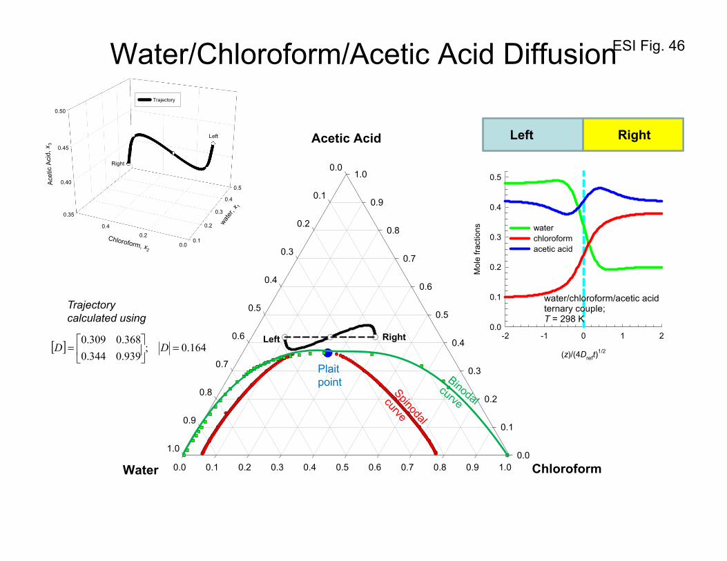
ESI Fig. 46

Chloroform0.0 0.1 0.2 0.3 0.4 0.5 0.6 0.7 0.8 0.9 1.0

Acetic Acid

0.0

0.1

0.2

0.3

0.4

0.5

0.6

0.7

0.8

0.9

1.0

Water

0.0

0.1

0.2

0.3

0.4

0.5

0.6

0.7

0.8

0.9

1.0

0.35

0.40

0.45

0.50

0.1

0.2

0.3

0.4

0.5

0.0

0.20.4

Ace

tic A

cid,

x3

water,

x 1Chloroform, x2

Trajectory

Left

Right

(z)/(4Dreft)1/2

-2 -1 0 1 2

Mol

e fra

ctio

ns

0.0

0.1

0.2

0.3

0.4

0.5

waterchloroformacetic acid

water/chloroform/acetic acidternary couple;T = 298 K

Water/Chloroform/Acetic Acid Diffusion

[ ] 164.0;939.0344.0

368.0309.0=

= DD

Left Right

Left Right

Trajectory calculated using

Plait point

ESI Fig. 47

Glycerol0.0 0.1 0.2 0.3 0.4 0.5 0.6 0.7 0.8 0.9 1.0

Water

0.0

0.1

0.2

0.3

0.4

0.5

0.6

0.7

0.8

0.9

1.0

Acetone

0.0

0.1

0.2

0.3

0.4

0.5

0.6

0.7

0.8

0.9

1.0

Plait point

glycerol(1)/acetone(2)/water(3);T = 298 K

Glycerol/Acetone/Water Equilibration

[ ] 1-29 s m10213.0148.0

127.0294.0 −×

=D

[ ] 1-29 s m10399.0458.0

227.0490.0 −×

=D

Simulation of trajectories using

Simulation of trajectories using

ESI Fig. 48

(z)/(4Dreft)1/2

-2 -1 0 1 2

Mol

e fra

ctio

n of

gly

cero

l, x 1

0.06

0.08

0.10

0.12

Activ

ity o

f gly

cero

l, γ 1 x

1

0.00

0.02

0.04

0.06

0.08

0.10

0.12

x1

γ1 x1

glycerol/acetone/water mixture;T = 298 K

activity of glycerol, γ1 x1

0.00 0.02 0.04 0.06 0.08 0.10

activ

ity o

f wat

er, γ

3 x3

0.20

0.25

0.30

0.35

0.40

0.45

0.50

0.55

0.60activitytrajectory

glycerol/acetone/water mixture;T = 298 K

eq

Mole fraction of glycerol, x1

0.04 0.06 0.08 0.10 0.12 0.14

Mol

e fra

ctio

n of

wat

er, x

3

0.25

0.30

0.35

0.40

0.45

0.50

0.55

0.60compositiontrajectoryBinodal curvePlait point

glycerol/acetone/water mixture;T = 298 K

eq

Glycerol/Acetone/Water Equilibration

(z)/(4Dreft)1/2

-2 -1 0 1 2

Mol

e fra

ctio

ns

0.0

0.1

0.2

0.3

0.4

0.5

0.6

glycerolacetonewater

glycerol/acetone/water mixture;T = 298 K

(a) (b)

(c) (d)

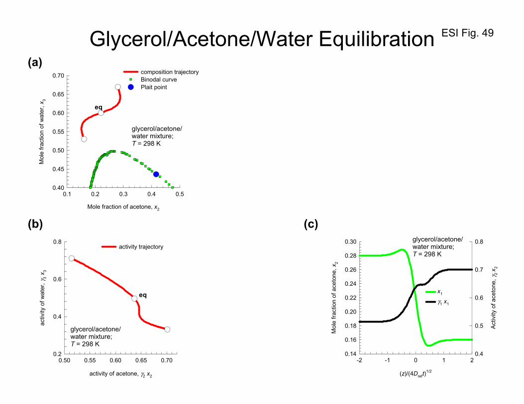
ESI Fig. 49

activity of acetone, γ2 x2

0.50 0.55 0.60 0.65 0.70

activ

ity o

f wat

er, γ

3 x3

0.2

0.4

0.6

0.8activity trajectory

glycerol/acetone/water mixture;T = 298 K

eq

Mole fraction of acetone, x2

0.1 0.2 0.3 0.4 0.5

Mol

e fra

ctio

n of

wat

er, x

3

0.40

0.45

0.50

0.55

0.60

0.65

0.70 composition trajectoryBinodal curvePlait point

glycerol/acetone/water mixture;T = 298 K

eq

Glycerol/Acetone/Water Equilibration(a)

(b) (c)

(z)/(4Dreft)1/2

-2 -1 0 1 2

Mol

e fra

ctio

n of

ace

tone

, x2

0.14

0.16

0.18

0.20

0.22

0.24

0.26

0.28

0.30

Act

ivity

of a

ceto

ne, γ

2 x 2

0.4

0.5

0.6

0.7

0.8

x1

γ1 x1

glycerol/acetone/water mixture;T = 298 K

ESI Fig. 50Water/Chloroform/Acetic Acid Diffusion

(z)/(4Dreft)1/2

-2 -1 0 1 2

Mol

e fra

ctio

ns

0.0

0.1

0.2

0.3

0.4

0.5

waterchloroformacetic acid

water/chloroform/acetic acidT = 298 K

Left Right

[ ] 0;161.037.0

4.092.0=

= DD

Trajectory calculated using

Mole fraction of chloroform, x2

0.0 0.1 0.2 0.3 0.4 0.5 0.6

Mol

e fra

ctio

n of

ace

tic a

cid,

x3

0.20

0.25

0.30

0.35

Dominant eigenvectorPlait point

water/chloroform/acetic acidT = 298 K

binodal curve

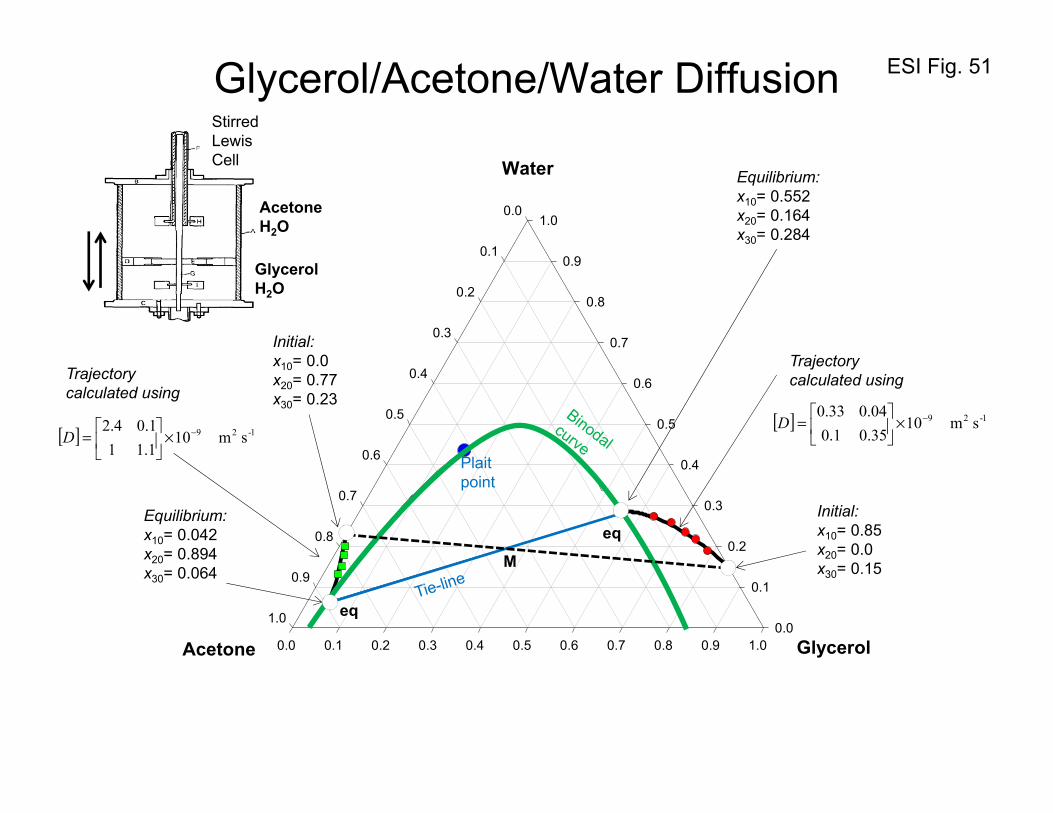
ESI Fig. 51

Glycerol0.0 0.1 0.2 0.3 0.4 0.5 0.6 0.7 0.8 0.9 1.0

Water

0.0

0.1

0.2

0.3

0.4

0.5

0.6

0.7

0.8

0.9

1.0

Acetone

0.0

0.1

0.2

0.3

0.4

0.5

0.6

0.7

0.8

0.9

1.0

Glycerol/Acetone/Water Diffusion

Plait point

Initial:x10= 0.0x20= 0.77x30= 0.23

eq

eqInitial:x10= 0.85x20= 0.0x30= 0.15

Equilibrium:x10= 0.042x20= 0.894x30= 0.064

Equilibrium:x10= 0.552x20= 0.164x30= 0.284

Trajectory calculated usingTrajectory

calculated using

M

[ ] 1-29 s m10

1.11

1.04.2 −×

=D

[ ] 1-29 s m1035.01.0

04.033.0 −×

=D

Stirred Lewis Cell

GlycerolH2O

AcetoneH2O

ESI Fig. 52

Mole fraction of glycerol

0.5 0.6 0.7 0.8

Mol

e fra

ctio

n of

wat

er

0.15

0.20

0.25

0.30

Experimentcoupled diffusion model

Krishna et al. 1985 Expt;glycerol/acetone/water mixtureT = 298 K

Transient trajectory to equilibrium

Initial composition

Equilibrium

Transient equilibration is captured by coupled Fick matrix

Please note that the component numbering is1 = glycerol2 = acetone3 = water

0.00

0.02

0.04

0.06

0.08

0.10

0.12

0.14

0.16

0.18

0.500.55

0.600.65

0.700.75

0.800.85

0.90

0.140.160.180.200.220.240.260.280.30

Mol

e fra

ctio

n ac

eton

e

Mole fr

actio

n glyc

erol

Mole fraction water

Model with couplingKrishna expt data

Krishna et al. 1985 Expt;glycerol/acetone/water mixtureT = 298 K

[ ] 1-29 s m1035.01.0

04.033.0 −×

=D

ESI Fig. 53

0.70

0.75

0.80

0.85

0.90

0.95

1.00

0.00

0.01

0.02

0.03

0.040.05

0.00.1

0.20.3

Mol

e fra

ctio

n ac

eton

e

Mole fr

actio

n glyc

erol

Mole fraction water

Model with couplingKrishna expt data

Krishna et al. 1985 Expt;glycerol/acetone/water mixtureT = 298 K

Mole fraction of glycerol

0.00 0.01 0.02 0.03 0.04

Mol

e fra

ctio

n of

wat

er

0.05

0.10

0.15

0.20

0.25Experimentcoupled diffusion model

Krishna et al. 1985 Expt;glycerol/acetone/water mixtureT = 298 K

Transient trajectory to equilibriumTransient equilibration is captured by coupled Fick matrix

Equilibrium

Initial composition

Please note that the component numbering is1 = glycerol2 = acetone3 = water

[ ] 1-29 s m10

1.11

1.04.2 −×

=D

ESI Fig. 54

water0.0 0.1 0.2 0.3 0.4 0.5 0.6 0.7 0.8 0.9 1.0

acetone

0.0

0.1

0.2

0.3

0.4

0.5

0.6

0.7

0.8

0.9

1.0

ethylacetate

0.0

0.1

0.2

0.3

0.4

0.5

0.6

0.7

0.8

0.9

1.0

binodalspinodal

acetone(1)/ethylacetate(2)/water(3);293 K These are experimental data points of Haeberl and

Blass.

Serpentine trajectory The simulations are performed with the values of the Fick diffusivity matrix corresponding to the thriddata point of Pertler

Acetone/Ethylacetate/Water: equilibration trajectory

[ ] 1-29 s m10764.0316.0

287.0179.0 −×

−=D

The phase diagram is drawn in mass fractions

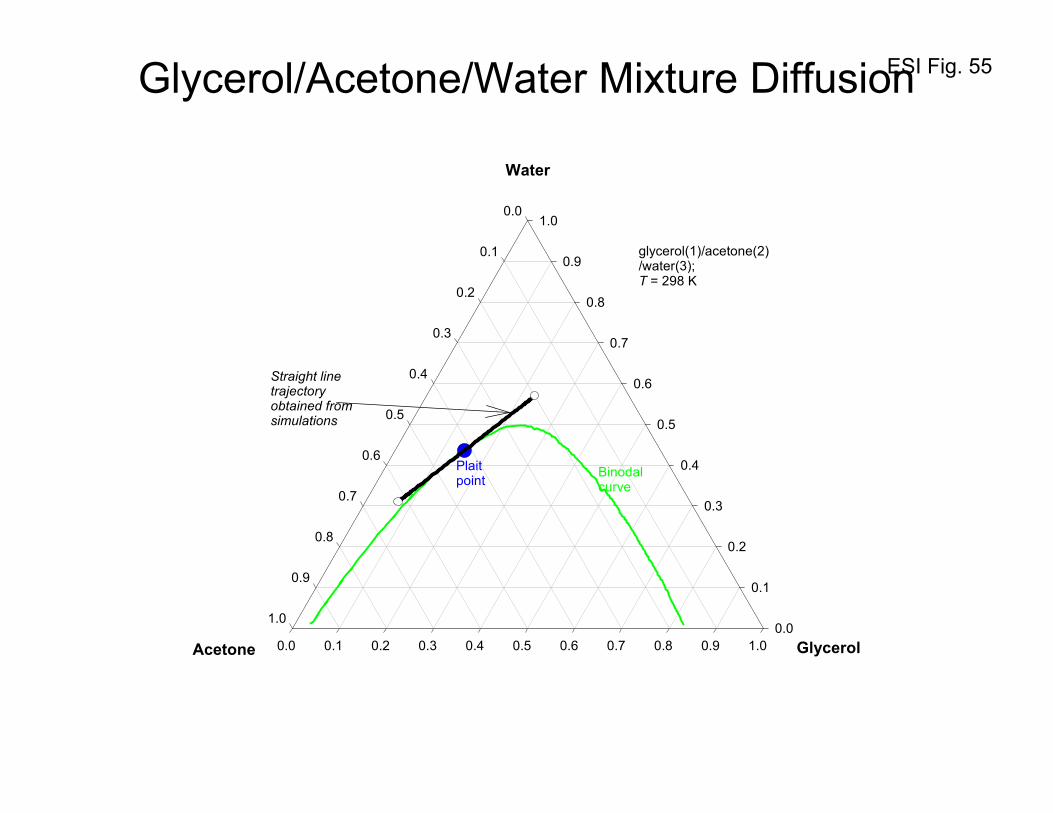
ESI Fig. 55Glycerol/Acetone/Water Mixture Diffusion

Glycerol0.0 0.1 0.2 0.3 0.4 0.5 0.6 0.7 0.8 0.9 1.0

Water

0.0

0.1

0.2

0.3

0.4

0.5

0.6

0.7

0.8

0.9

1.0

Acetone

0.0

0.1

0.2

0.3

0.4

0.5

0.6

0.7

0.8

0.9

1.0

Plait point

Straight linetrajectoryobtained from simulations

Binodalcurve

glycerol(1)/acetone(2)/water(3);T = 298 K

ESI Fig. 56The Ouzo Effect

trans-anethol

0.0 0.1 0.2 0.3 0.4 0.5 0.6 0.7 0.8 0.9 1.0

ethanol

0.0

0.1

0.2

0.3

0.4

0.5

0.6

0.7

0.8

0.9

1.0

water

0.0

0.1

0.2

0.3

0.4

0.5

0.6

0.7

0.8

0.9

1.0

Observation: Addition of water to Ouzo results in a meta-stable dispersion.

45% vol ethanol55% vol water≈ 0.1% vol trans-anethol

Cloudy meta-table Ouzo zone

Add water inratio 5:1 Question: What

causes the equilibration trajectory to enter the meta-stable zone? Uphill transport of water?

ESI Fig. 57

Sitnikova Expt;trans-anethol/ethanol/water mixtureT = 298 K

Mass fraction of trans-anethol

0.00 0.02 0.04 0.06 0.08 0.10

Mas

s fra

ctio

n of

wat

er

0.0

0.1

0.2

0.3

0.4

0.5

0.6

0.7

0.8

0.9

1.0

Binodal curve"neat" Ouzo

Equilibration trajectory – Ouzo effect

Add water in ratio 5:1

45% vol ethanol55% vol water≈ 0.1% vol trans-anethol

This must lie in the meta-stable region between the binodal and spinodalenvelopes

Ruschak-Miller straight line equilibration for addition of water to neat Ouzo

Does the equilibration follow a curvilinear trajectory?

ESI Fig. 58

Toluene0.0 0.1 0.2 0.3 0.4 0.5 0.6 0.7 0.8 0.9 1.0

Ethanol

0.0

0.1

0.2

0.3

0.4

0.5

0.6

0.7

0.8

0.9

1.0

Water

0.0

0.1

0.2

0.3

0.4

0.5

0.6

0.7

0.8

0.9

1.0

spinodalbinodal

A B

C

D

E

Linear and Serpentine Trajectories

Serpentine trajectory entersthe meta-stable zone; may

result in spontaneous emulsification.

Serpentine trajectory enters the two-phase zone that will result in spinodaldecomposition.

Linear trajectory remains in the homogenous phase region.

Linear trajectory enters the meta-stable region. So spontaneous emulsification can occur

The phase diagram is drawn in mass fractions

These are not simulated trajectories, just scenarios that are possible.

ESI Fig. 59

Chloroform0.0 0.1 0.2 0.3 0.4 0.5 0.6 0.7 0.8 0.9 1.0

Acetic Acid

0.0

0.1

0.2

0.3

0.4

0.5

0.6

0.7

0.8

0.9

1.0

Water

0.0

0.1

0.2

0.3

0.4

0.5

0.6

0.7

0.8

0.9

1.0

Plait pointBinodal curveSpinodal curve

(z)/(4Dreft)1/2

-2 -1 0 1 2

Mol

e fra

ctio

ns

0.1

0.2

0.3

0.4

0.5

waterchloroformacetic acid

water/chloroform/acetic acid;T = 298 K

Water/Chloroform/Acetic Acid Diffusion

Serpentine trajectory obtained with

predicts possibility of emulsification

[ ] 164.0;939.0344.0

368.0309.0=

= DD

Linear equilibration trajectory: no emulsification

Left Right

Plait point

Mole fraction of chloroform, x2

0.0 0.1 0.2 0.3 0.4

Mol

e fra

ctio

n of

ace

tic a

cid,

x3

0.25

0.30

0.35

0.40

0.45

0.50 water/chloroform/acetic acidT = 298 K

eq

spinodal curve

binodal curve

Meta-stable region between binodaland spinodalenvelopes

ESI Fig. 60Water/Chloroform/Acetic Acid Diffusion

Mole fraction of water

0.0 0.2 0.4 0.6

Mol

e fra

ctio

n of

chl

orof

orm

0.0

0.1

0.2

0.3

0.4

coupled diffusion trajectory

water/chloroform/acetic acidternary couple;T = 298 K

fast eigenvector

sloweigenvector

fast eigenvector

ESI Fig. 61

water0.0 0.1 0.2 0.3 0.4 0.5 0.6 0.7 0.8 0.9 1.0

acetone

0.0

0.1

0.2

0.3

0.4

0.5

0.6

0.7

0.8

0.9

1.0

ethylacetate

0.0

0.1

0.2

0.3

0.4

0.5

0.6

0.7

0.8

0.9

1.0

spinodalbinodal

acetone(1)/water(2)/ethylacetate(3);T = 293 K

(z)/(4Dreft)1/2

-4 -3 -2 -1 0 1 2 3 4

Mas

s fra

ctio

ns

0.0

0.1

0.2

0.3

0.4

0.5

0.6

0.7

0.8

waterethylacetateacetone

Mass fraction of water

0.00 0.02 0.04 0.06 0.08 0.10

Mas

s fra

ctio

n of

eth

ylac

etat

e

0.68

0.70

0.72

0.74

0.76

0.78

0.80

0.82

eq

binodal curve

Acetone/Water/Ethylacetate: equilibration trajectory

Serpentine trajectory enters the meta-stable zone.

The simulations are performed with the values of the Fick diffusivity matrix corresponding to the sixth data point of Pertler

The phase diagram is drawn in mass fractions

[ ] 1-29 s m10016.647.17

298.0371.1 −×

−

=D

ESI Fig. 62

mole fraction of water, x1

0.0 0.1 0.2 0.3 0.4 0.5 0.6 0.7

mol

e fra

ctio

n of

2-p

ropa

nol,

x 2

0.0

0.1

0.2

0.3

0.4

0.5

0.6

0.7

Plait pointT = 303.75 KT = 304.15 KT = 304.65 KT = 306.65 K

water(1)/2-propanol(2)/cyclohexane(3)

binodalcurve

Water/2-propanol/cyclohexane mixture diffusion

[ ] 847.4;064.1997.0

547.0467.0=

−−

= DD

[ ] 921.0;571.0566.0

328.0309.0=

−−

= DD

[ ] 466.0;439.0440.0

267.0257.0=

−−

= DD

[ ] 359.0;510.0559.0

323.0347.0=

−−

= DD

Units: 10-10 m2 s-1

Units: 10-18 m4 s-2

ESI Fig. 63

Toluene0.0 0.1 0.2 0.3 0.4 0.5 0.6 0.7 0.8 0.9 1.0

Acetone

0.0

0.1

0.2

0.3

0.4

0.5

0.6

0.7

0.8

0.9

1.0

Water

0.0

0.1

0.2

0.3

0.4

0.5

0.6

0.7

0.8

0.9

1.0

BinodalSpinodalPlait point

water(1)/acetone(2)/toluene(3);T = 298 K

Mole fraction of toluene x3

0.0 0.1 0.2 0.3 0.4

Mol

e fra

ctio

n of

ace

tone

, x2

0.50

0.55

0.60

0.65water(1)/acetone(2)/toluene(3);T = 298 K

eq

spinodal curve

binodal curve

Plait point:Water = 0.4762Acetone = 0.4762Toluene = 0.04762

Water/Acetone/Toluene diffusion

Serpentine trajectory does not enter the meta-stable zone.

The simulations are performed with the values of the Fick diffusivity matrix that are estimated to be

[ ] 1-29 s m1038.2574.0

29.119.0 −×

−−=D

ESI Fig. 64

Toluene0.0 0.1 0.2 0.3 0.4 0.5 0.6 0.7 0.8 0.9 1.0

Ethanol

0.0

0.1

0.2

0.3

0.4

0.5

0.6

0.7

0.8

0.9

1.0

Water

0.0

0.1

0.2

0.3

0.4

0.5

0.6

0.7

0.8

0.9

1.0

binodalspinodal

toluene(1)/ethanol(2)/water(3);T = 298 K

Toluene/ethanol/water equilibration

The simulations are performed with the values of the Fick diffusivity matrix that are estimated to be

[ ] 1-29 s m1053.06.2

1.06.0 −×

−

−=D

Mole fraction of toluene x1

0.00 0.01 0.02 0.03

Mol

e fra

ctio

n of

wat

er, x

3

0.60

0.65

0.70

0.75

0.80

0.85

0.90

0.95

1.00

toluene(1)/ethanol(2)/water(3);T = 298 K

spinodal curve

binodal curve

ESI Fig. 65

Mole fraction of water, x1

0.30.40.50.60.70.80.9

Mol

e fra

ctio

n of

cap

rola

ctam

, x2

0.10

0.15

0.20

0.25

0.30

0.35 binodal curveplait pointspinodal curve

water(1)/caprolactam(2)/toluene(3) mixture;T = 298 K

eq

spinodal curve

binodal curve

toluene0.0 0.1 0.2 0.3 0.4 0.5 0.6 0.7 0.8 0.9 1.0

Caprolactam

0.0

0.1

0.2

0.3

0.4

0.5

0.6

0.7

0.8

0.9

1.0

water

0.0

0.1

0.2

0.3

0.4

0.5

0.6

0.7

0.8

0.9

1.0

spinodalbinodalplait point

water(1)/caprolactam(2)/toluene(3) mixture;T = 298 K

Water/Caprolactam/Toluene Emulsification

Linear equilibration trajectory: no emulsification

Plait point

Serpentine trajectory obtained with

predicts possibility of emulsification

[ ] 1-29 s m1010.242.0

52.1176.0 −×

−−=D

ESI Fig. 66

Mole fraction of water, x1

0.00.10.20.30.4

Mol

e fra

ctio

n of

cap

rola

ctam

, x2

0.00

0.05

0.10

0.15

0.20

0.25

0.30binodal curveplait pointspinodal curve

eq

water(1)/caprolactam(2)/benzene(3) mixture;T = 298 K

spinodal curve

binodal curve

benzene0.0 0.1 0.2 0.3 0.4 0.5 0.6 0.7 0.8 0.9 1.0

Caprolactam

0.0

0.1

0.2

0.3

0.4

0.5

0.6

0.7

0.8

0.9

1.0

water

0.0

0.1

0.2

0.3

0.4

0.5

0.6

0.7

0.8

0.9

1.0

spinodalbinodalplait point

water(1)/caprolactam(2)/benzene(3) mixture;T = 298 K

Water/Caprolactam/Benzene Emulsification

Linear equilibration trajectory: no emulsification

Plait point

Serpentine trajectory obtained with

predicts possibility of emulsification

[ ] 1-29 s m1011.2878.0

925.0591.0 −×

−

−=D

ESI Fig. 67

water0.0 0.1 0.2 0.3 0.4 0.5 0.6 0.7 0.8 0.9 1.0

propionic acid

0.0

0.1

0.2

0.3

0.4

0.5

0.6

0.7

0.8

0.9

1.0

toluene

0.0

0.1

0.2

0.3

0.4

0.5

0.6

0.7

0.8

0.9

1.0

binodalspinodal

toluene(1)/propionic acid(2)/water(3);T = 298 K

binodal curve

spinodal curve

Toluene//Propionic acid/Water Emulsification

Linear equilibration trajectory: no emulsification

Serpentine trajectory obtained with

predicts possibility of emulsification

Mole fraction of water x3

0.1 0.2 0.3 0.4 0.5

Mol

e fra

ctio

n of

pro

pion

ic a

cid,

x2

0.00

0.05

0.10

0.15

0.20

0.25

0.30

eq

spinodal curve

binodal curve

toluene(1)/water(2)/propionic acid(3);T = 298 K

[ ] 1-29 s m101.19580.1806

0.2963-0.3267 −×

=D

ESI Fig. 68

water0.0 0.1 0.2 0.3 0.4 0.5 0.6 0.7 0.8 0.9 1.0

propionic acid

0.0

0.1

0.2

0.3

0.4

0.5

0.6

0.7

0.8

0.9

1.0

Ethylacetate

0.0

0.1

0.2

0.3

0.4

0.5

0.6

0.7

0.8

0.9

1.0

binodalspinodal

ethylacetate(1)/propionic acid(2)/water(3);T = 298 K

binodal curve

spinodal curve

Ethylacetate/Propionic acid/Water Emulsification

Mole fraction of water x3

0.0 0.1 0.2 0.3 0.4

Mol

e fra

ctio

n of

pro

pion

ic a

cid,

x2

0.00

0.05

0.10

0.15

0.20

eq

spinodal curvebinodal

curve

ethylacetate(1)/propionic acid(2)/water(3);T = 298 K

Linear equilibration trajectory: no emulsification

Serpentine trajectory obtained with

predicts possibility of emulsification

[ ] 1-29 s m103.63790.5700

1.7447-0.0358- −×

=D

ESI Fig. 69Membrane formation

water

Cellulose Acetate

Acetone

Meta-stable region

t = 10 s

t = 25 st = 50 s

Two liquid phases

t = 0 s 10% CA solution Plait

point

EQ

Water bath

10% CA/90% Acetone

support

ESI Fig. 70

wt % water

0 20 40 60 80 100

(ace

tone

diffu

sivi

ty)/(

wat

er d

iffus

ivity

)

10-4

10-3

10-2

10-1

100

in coffee extractin maltro dextrin

Coumans et al

wt % water

0 20 40 60 80 100

Diff

usiv

ity /

m2 s

-1

10-15

10-14

10-13

10-12

10-11

10-10

10-9

acetone in malto-dextrinwater in malto-dextrinwater in coffee extrractacetone in coffee extract

Coumans et al

Drying of food liquids

(a) (b)

water

acetone

maltodextrin

ESI Fig. 71

Distance from weld interface / mm

-20 -10 0 10 20

wt %

C

0.3

0.4

0.5

0.6

Coupled diffusion modelDarken expt data

Darken expt;C/Si/Fe ternary couple;time = 13 days; T = 1323 K

wt% Si

0 1 2 3 4

wt %

C

0.3

0.4

0.5

0.6

Coupled diffusion trajectoryDarken expt data

Darken expt;C/Si/Fe ternary couple;time = 13 days; T = 1323 K

Classic Darken Experiments

Right0.45% C0.05% Si99.50% Fe

Left0.48% C3.80% Si95.72% Fe

Fick diffusivity matrixused in the simulations

(a)(b)

[ ] 1-213 s m103.20

34480 −×

=D

Left0.48% C3.80% Si

95.72% Fe

Right0.45% C0.05% Si

99.50% Fe

Higher C content near the surface results in surface hardening

High C = Hard Bulk = ToughHigher activity of C

Lower activity of C

ESI Fig. 72Cu(1)/Ag(2)/Au(3) equilibration: Ziebold

Ag0.0 0.1 0.2 0.3 0.4 0.5 0.6 0.7 0.8 0.9 1.0

Au

0.0

0.1

0.2

0.3

0.4

0.5

0.6

0.7

0.8

0.9

1.0

Cu

0.0

0.1

0.2

0.3

0.4

0.5

0.6

0.7

0.8

0.9

1.0

Cu(1)/Ag(2)/Au(3);T = 998 K

(z)/(4Dreft)1/2

-4 -3 -2 -1 0 1 2 3 4

Ato

m fr

actio

ns

0.0

0.2

0.4

0.6

0.8

1.0

Cu(1)Ag(2)Au(3)

Cu(1)/Ag(2)/Au(3);T = 998 K

Fick diffusivity matrixused in the simulations

[ ] 1-214 s m101.38.1

11.13.2 −×

=D

ESI Fig. 73Uphill diffusion in glasses

Glass R22.8% K2O15.6% SrO61.6% SiO2

Glass L18.1% K2O18.0% SrO63.9% SiO2

Fick diffusivity matrix

[ ] 1-213 s m1033.022.1

267.01 −×

−

−=D

(a)

(b)

61.0

61.5

62.0

62.5

63.0

63.5

64.0

64.5

65.0

15

20

25

30

1516

1718

% S

iO2

% K 2

O

% SrO

Fick [D] Uncoupled diffusionVarshneya experiments

Varshneya and CooperK2O/SrO/SiO2 mixturetime = 4.55 h; T = 1071 K

Distance from interface / μm

-150 -100 -50 0 50 100 150

wt %

15

16

17

18

19

20

21

22

23

24

MatanoplaneK2OSrO

Varshneya and CooperK2O/SrO/SiO2 mixturetime = 4.55 h; T = 1071 K

Glass22.8% K2O15.6% SrO61.6% SiO2

Glass18.1% K2O18.0% SrO63.9% SiO2

ESI Fig. 74

Fe0 10 20 30 40 50 60 70 80 90 100

Mg

0

10

20

30

40

50

60

70

80

90

100

Ca

0

10

20

30

40

50

60

70

80

90

100

trajectory followed in Vielzeuf experimentsTrajectory followed for uncoupled diffusion

Vielzeuf & Saul;Fe/Mg/Ca ternary couple;time = 100 h; T = 1423 K

Fe/Mg/Ca diffusion couple

Distance from interface / μm

-3 -2 -1 0 1 2 3

atom

% F

e, M

g, C

a

0

10

20

30

40

50

FeMgCa

Vielzeuf & Saul;Fe/Mg/Ca ternary couple;time = 100 h; T = 1423 K

Left 35.85 % Fe47.00 % Mg17.15 % Ca

Right50.85 % Fe46.00 % Mg3.15 % Ca

Left

Right

(a) (b)

ESI Fig. 75

Distance from interface / μm

-3 -2 -1 0 1 2 3

atom

% F

e, M

g, C

a

0

10

20

30

40

50

FeMgCa

Vielzeuf & Saul;Fe/Mg/Ca ternary couple;time = 100 h; T = 1423 K

2

4

6

8

10

12

14

16

18

3436

3840

4244

4648

5052

4244

4648

50

% C

a

% F

e

% Mg

Coupled diffusionUncoupled diffusionVielzeuf expt data

Vielzeuf & Saul;Fe/Mg/Ca ternary couple;time = 100 h; T = 1423 K

Ternary Diffusion Couple

Left 35.85 % Fe47.00 % Mg17.15 % Ca

Fick diffusivity matrix used in the simulations

(a)

(b)

Right50.85 % Fe46.00 % Mg3.15 % Ca

[ ] 1-219 s m1018.15.5

02.186.5 −×

−

−=D

Left 35.85 % Fe47.00 % Mg17.15 % Ca

Right50.85 % Fe46.00 % Mg3.15 % Ca

ESI Fig. 76

Mass transfer in distillation

Vapor leavingV, yL

VaporenteringV, yE

Liquid leavingL, xL

Liquid enteringL, xE

Vapor Liquid

Diffusional coupling effects need to be accounted for in either phase

ESI Fig. 77

Stage number

0 2 4 6 8 10 12

Eth

anol

driv

ing

forc

e, (y

2* -

y 2E )

-0.25

-0.20

-0.15

-0.10

-0.05

0.00

0.05

ethanol

Springer et al.water/ethanol/acetone

(b)(c)

(c)

Murphree component efficiencies

Stage number

0 2 4 6 8 10 12

Mur

phre

e co

mpo

nent

effi

cien

cies

-2.0

-1.5

-1.0

-0.5

0.0

0.5

1.0

waterethanolacetone

Springer et al.water/ethanol/acetone

ESI Fig. 78

Water0.0 0.1 0.2 0.3 0.4 0.5 0.6 0.7 0.8 0.9 1.0

Ethanol

0.0

0.1

0.2

0.3

0.4

0.5

0.6

0.7

0.8

0.9

1.0

Acetone

0.0

0.1

0.2

0.3

0.4

0.5

0.6

0.7

0.8

0.9

1.0

Residue curvesAzeotropeDistillation boundaryexpt data

Springer et al.water/ethanol/acetone

373.2 K329.7 K

351.6 K

Crossing distillation boundaries

mole fraction, water

0.0 0.1 0.2 0.3

mol

e fra

ctio

n, e

than

ol

0.2

0.4

0.6

0.8

1.0

Distillation boundaryExpt data

EQ model

NEQmodel

mole fraction, water

0.00 0.02 0.04 0.06

mol

e fra

ctio

n, e

than

ol

0.2

0.4

0.6

0.8

1.0

Distillation boundaryExpt data

EQmodel

NEQmodel

(b) (a) (c)

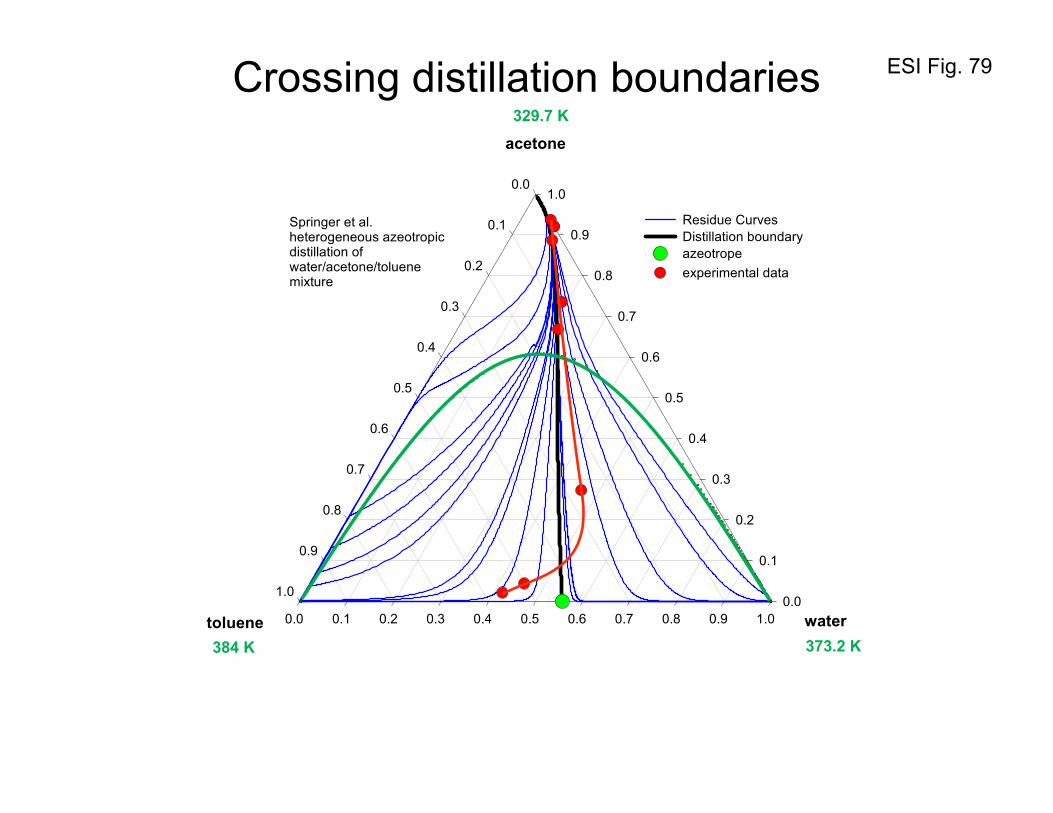
ESI Fig. 79Crossing distillation boundaries

water0.0 0.1 0.2 0.3 0.4 0.5 0.6 0.7 0.8 0.9 1.0

acetone

0.0

0.1

0.2

0.3

0.4

0.5

0.6

0.7

0.8

0.9

1.0

toluene

0.0

0.1

0.2

0.3

0.4

0.5

0.6

0.7

0.8

0.9

1.0

Residue CurvesDistillation boundaryazeotropeexperimental data

Springer et al.heterogeneous azeotropicdistillation ofwater/acetone/toluenemixture

373.2 K384 K

329.7 K

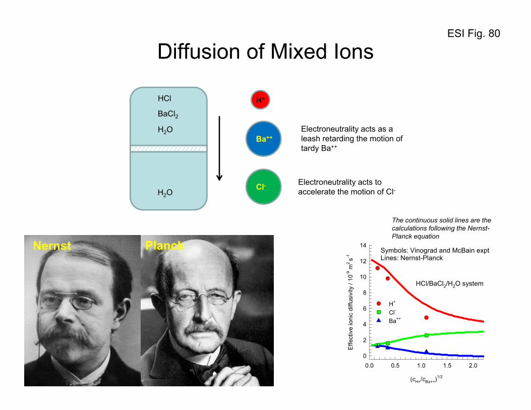
ESI Fig. 80

Diffusion of Mixed Ions

Nernst Planck

HCl

BaCl2

H2O

H2O

H+

Ba++

Cl-

Electroneutrality acts as a leash retarding the motion of tardy Ba++

Electroneutrality acts to accelerate the motion of Cl-

(cH+/cBa++)1/2

0.0 0.5 1.0 1.5 2.0

Effe

ctiv

e io

nic

diffu

sivi

ty /

10-9

m2 s-1

0

2

4

6

8

10

12

14

H+

Cl-

Ba++

HCl/BaCl2/H2O system

Symbols: Vinograd and McBain exptLines: Nernst-Planck

The continuous solid lines are the calculations following the Nernst-Planck equation

ESI Fig. 81

Asymmetry in Ion-Exchange Kinetics

time, t / h

0 5 10 15 20 25

Frac

tiona

l upt

ake

0.0

0.2

0.4

0.6

0.8

1.0 initially H+ in solutioninitially H+ in ion-exchanger

Lewatit S100 ion exchanger

Na+

H+

Na+

H+

ESI Fig. 82

Transport across cation-exchange

membrane

time, t / h

0 20 40 60

H+ a

nd N

a+ con

cent

ratio

ns, c

i / m

ol L

-1

0.00

0.05

0.10

0.15

Cs+ c

once

ntra

tion,

ci /

mol

L-1

0.000

0.002

0.004

0.006

H+ in salt compartmentNa+ in acid compartmentCs+ in acid compartment

Yang & Pintauro Expt

NafionCationExchange Membrane

Na+

Cs+

H+

SO42-

Salt compartment0.125 M Na2SO40.0054 M Cs2SO4

Acid Compartment0.125 M H2SO4

HSO4-

ESI Fig. 83

Reverse osmosis

open support structure

Salt water

Polyamide thin fim

water

Appliedpressure

Desalinatedwater

wMt

ww

ww

Ðc

N

dz

dpV

RTdz

d

RT

x =−− 1μ

ESI Fig. 84Microporous materials: 1D channels

MgMOF-74

AFI

MIL-53(Cr)-lp

BTP-COF

Fe2(BDP)3

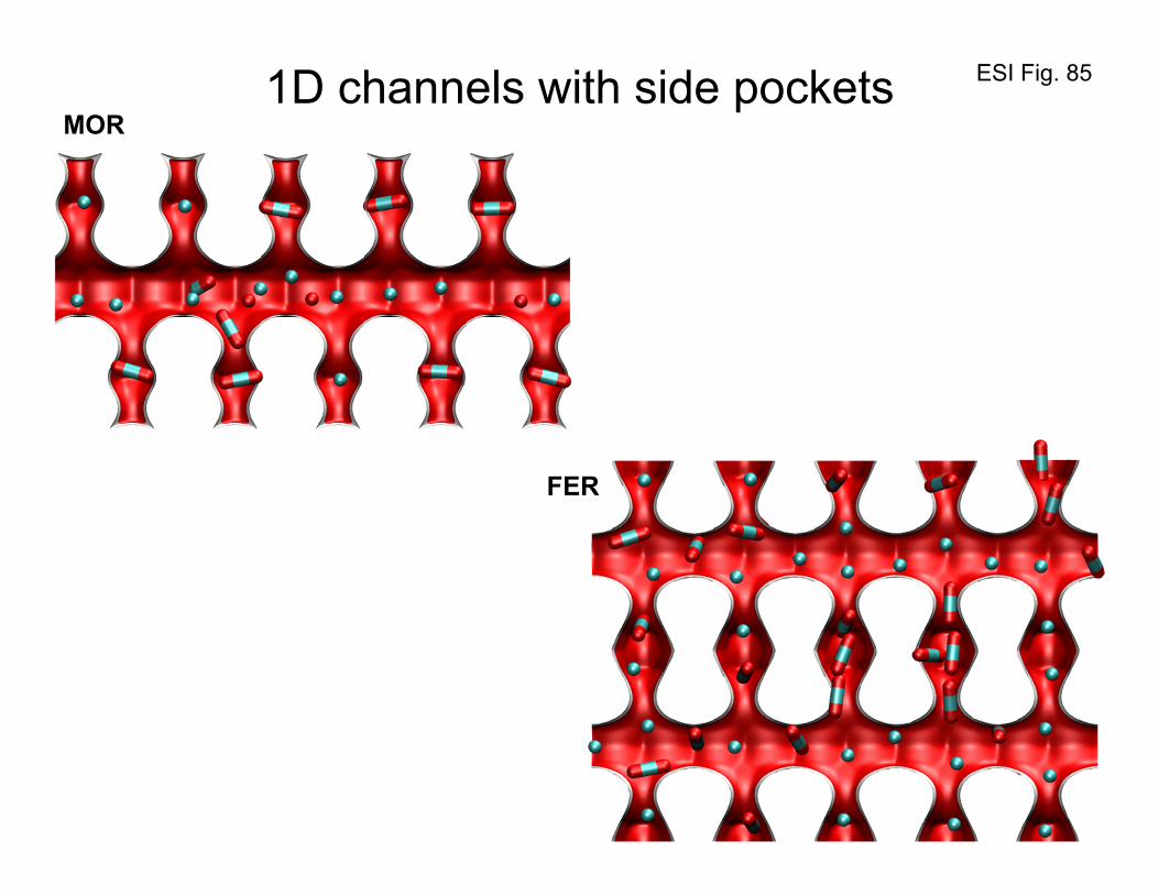
ESI Fig. 851D channels with side pocketsMOR

FER

ESI Fig. 86Intersecting channels

MFIZn(bdc)dabco

ESI Fig. 87

LTA

CHA

DDR

ZIF-8

Cages with narrow windows

ESI Fig. 88Cages with large windowsIRMOF-1

CuBTC

FAU

ESI Fig. 89PSA separations for O2/N2

N2

O2

Na+

LTA-4A (96 Na+ per uc)

t1/2 / min1/2

0.0 0.5 1.0

Dim

ensi

onle

ss c

once

ntra

tion

at o

utle

t, c i /

ci0

0.0

0.5

1.0

nitrogen, (DN2/rc2) = 2x10-5 s-1

oxygen, (DO2/rc2) = 2x10-3 s-1

oxygen/nitrogen mixture;p1= 42 kPa;p2= 158 kPa;LTA-4A; 298 K

Ð1/Ð2 = 100;b2/b1 = 2

Partial blocking of window apertureby cations

O O

4.3 Å

3.1

Å

N N4.4 Å

3.3

Å

ESI Fig. 90

upstream compartment

downstream compartment

q10

q1δq20

q2δ

Δq1= q10-q1δΔq2= q20-q2δ

Component 1

Component 2

N2

N1

p10, p20 p1δ, p2δ

Δp1= p10-p1δΔp2= p20-p2δ

Membrane separation

Por

ous

Cry

stal

line

laye

r

Sup

port

laye

r

Component 1

Component 2

N2

N1

δ

ESI Fig. 91

Fractional occupancy, θi

0.0 0.2 0.4 0.6 0.8 1.0

Inve

rse

ther

mod

ynam

ic fa

ctor

, 1/Γ

i

0.0

0.2

0.4

0.6

0.8

1.0

1/Γi

Thermodynamic Factor: unary adsorption

Fractional occupancy, θi

0.0 0.2 0.4 0.6 0.8 1.0

Ther

mod

ynam

ic c

orre

ctio

n fa

ctor

, Γi

0

2

4

6

8

101/(1-θi)

(a) (b)

ESI Fig. 92

t1/2 / min1/2

0 1 2 3 4

Frac

tiona

l app

roac

h to

equ

ilibr

ium

0.0

0.2

0.4

0.6

0.8

1.0

Di/rc2 = 1.1 x 10-3 s-1

Di/rc2 = 6 x 10-4 s-1

adsorption cycle, Exptdesorption cycle, Expt

C2H6 in LTA-4A;298 K

Na+

LTA-4A (96 Na+)

Adsorption/Desorption asymmetry

Partial blocking of window apertureby cations

ESI Fig. 93

p-xylene

t1/2 / min1/2

0 1 2 3 4 5

p- x

ylen

e lo

adin

g / m

ol k

g-1

0.0

0.1

0.2

0.3

0.4

0.5

Adsorption:p1 = 0 Pa to 115 PaDesorption:p1 = 115 Pa to 0 Pa

p-Xylene;H-ZSM-5; 375 K;Niessen & Karge

Adsorption/Desorption asymmetry

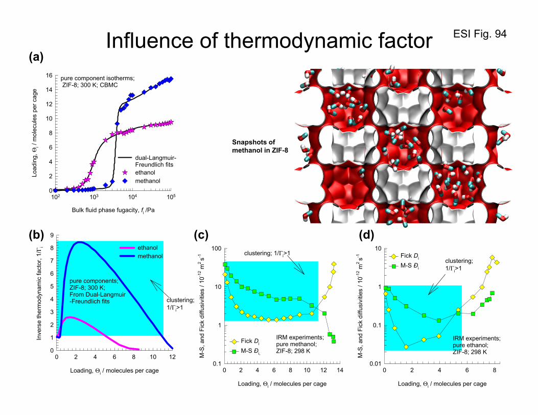
ESI Fig. 94Influence of thermodynamic factor

Bulk fluid phase fugacity, fi /Pa

102 103 104 105

Load

ing,

Θi /

mol

ecul

es p

er c

age

0

2

4

6

8

10

12

14

16

dual-Langmuir-Freundlich fitsethanolmethanol

pure component isotherms; ZIF-8; 300 K; CBMC

Loading, Θi / molecules per cage

0 2 4 6 8 10 12

Inve

rse

ther

mod

ynam

ic fa

ctor

, 1/Γ

i

0

1

2

3

4

5

6

7

8

9

ethanolmethanol

pure components; ZIF-8; 300 K;From Dual-Langmuir-Freundlich fits clustering;

1/Γi>1

Loading, Θi / molecules per cage

0 2 4 6 8 10 12 14

M-S

, and

Fic

k di

ffusi

vitie

s / 1

0-12 m

2 s-1

0.1

1

10

100

Fick Di

M-S Ði,

IRM experiments;pure methanol; ZIF-8; 298 K

clustering; 1/Γi>1

Loading, Θi / molecules per cage

0 2 4 6 8

M-S

, and

Fic

k di

ffusi

vitie

s / 1

0-12 m

2 s-1

0.01

0.1

1

10Fick Di

M-S Ðiclustering;1/Γi>1

IRM experiments;pure ethanol; ZIF-8; 298 K

(c)

(a)

(d)

Snapshots of methanol in ZIF-8

(b)

ESI Fig. 95N2/CH4 mixture uptake in LTA-4A

t1/2 / min1/2

0 25 50 75 100

Com

pone

nt lo

adin

g / m

ol k

g-1

0.0

0.5

1.0

1.5

2.0

2.5 N2

CH4

LTA-4A; 194 KBulk vapour:pN2 = 50.9 kPa;pCH4 = 49.1 kPa;Habgood expt data

Na+

LTA-4A (96 Na+ per uc)

CH4 uptake/ mol kg-1

0.0 0.5 1.0 1.5 2.0 2.5

N2 u

ptak

e/ m

ol k

g-1

0.0

0.5

1.0

1.5

2.0

2.5 Habgood expt data

LTA-4A; 194 K;pN2 = 50.9 kPa; pCH4 = 49.1 kPa;

Partial blocking of window apertureby cations

3.3 Å

4.4 Å

3.7 Å

3.7 Å

N N

CH4

ESI Fig. 96

Thermodynamic factors N2/CH4 in LTA-4A(b)(a)

Total mixture loading, qt / mol kg-1

0 1 2 3Ther

mod

ynam

ic c

orre

ctio

n fa

ctor

s, Γ

11, Γ

12, Γ

21, Γ

22

0.01

0.1

1

10Γ11

Γ22

Γ12

Γ22

N2(1)/CH4(2) mixture; p1=p2;Calculations from mixed gas Langmuir;194 K; LTA-4A

t1/2 / min1/2

0 5 10 15 20 25 30Ther

mod

ynam

ic c

orre

ctio

n fa

ctor

s, Γ

11, Γ

12, Γ

21, Γ

22

0.01

0.1

1

10

Γ11

Γ22

Γ12

Γ21

N2(1)/CH4(2) mixture; p1=p2;194 K; LTA-4A

(c)

t1/2 / min1/2

0 20 40 60 80 100Th

erm

odyn

amic

ally

"cor

rect

ed" l

oadi

ngs

10

20

30

40

N2 : Γ11q1+ Γ12q2

CH4: Γ21q1+ Γ22q2

N2(1)/CH4(2) mixture; p1=p2;194 K; LTA-4A

ESI Fig. 97

0

20

40

60

80

100

0.0

0.5

1.0

1.5

2.0

2.5

0.00.5

1.01.5

2.02.5

t1/2 /

min

1/2

CH 4 up

take /

mol kg

-1

N2 uptake /mol kg -1

Habgood expt dataModel with thermodynamic couplingUncoupled diffusion

N2/CH4 mixture uptake LTA-4A

CH4 uptake/ mol kg-1

0.0 0.5 1.0 1.5 2.0 2.5

N2 u

ptak

e/ m

ol k

g-1

0.0

0.5

1.0

1.5

2.0

2.5

Habgood expt dataCoupled diffusionuncoupled diffusion

LTA-4A; 194 K;pN2 = 50.9 kPa; pCH4 = 49.1 kPa;

Ð1/Ð2 = 22;b2/b1 = 2.2

t1/2 / min1/2

0 25 50 75 100

Com

pone

nt lo

adin

g / m

ol k

g-1

0.0

0.5

1.0

1.5

2.0

2.5

expt data N2

expt data CH4

N2, with Γij

CH4, with Γij

Dashed lines indicatesimulations for whichΓij is assumed to be δij

LTA-4A; 194 K;pN2 = 50.9 kPa;pCH4 = 49.1 kPa;

ESI Fig. 98

CH4 uptake/ mol kg-1

0.0 0.5 1.0 1.5 2.0 2.5

N2 u

ptak

e/ m

ol k

g-1

0.0

0.5

1.0

1.5

2.0

2.5

Habgood expt dataSimulation of adsorptionSimulation of desorption

LTA-4A; 194 K;pN2 = 50.9 kPa; pCH4 = 49.1 kPa;

Ð1/Ð2 = 22;b2/b1 = 2.2

Adsorption-Desorption Asymmetry

(b)(a)

t1/2 / min1/2

0 25 50 75 100

Com

pone

nt lo

adin

g / m

ol k

g-1

0.0

0.5

1.0

1.5

2.0

2.5

N2

CH4

Ð1/Ð2 = 22;b2/b1 = 2.2

LTA-4A; 194 K;pN2 = 50.9 kPa; pCH4 = 49.1 kPa;

ESI Fig. 99

Dimensionless time, τ = t u / ε L

0.1 1 10 100 1000 10000

Dim

ensi

onle

ss c

once

ntra

tion

at o

utle

t, c i /

ci0

0.0

0.2

0.4

0.6

0.8

1.0CH4

N2

N2(1)/CH4(2);p1= 10 kPa; p2= 90 kPa;LTA-4A; 194 K

Ð1/Ð2 = 22;b2/b1 = 2.2

Separations of N2/CH4 mixtures in PSA unit

N2

CH4

Na+

LTA-4A (96 Na+ per uc)

Partial blocking of window apertureby cations

Inlet gas contains 10% N2

Dimensionless time, τ = t u / ε L

0.1 1 10 100 1000 10000

% c

ompo

nent

gas

at o

utle

t0

20

40

60

80

100

CH4

N2

N2(1)/CH4(2);p1= 10 kPa; p2= 90 kPa;LTA-4A; 194 K

Ð1/Ð2 = 22;b2/b1 = 2.2

Nearly pure CH4 can be recovered during this time interval

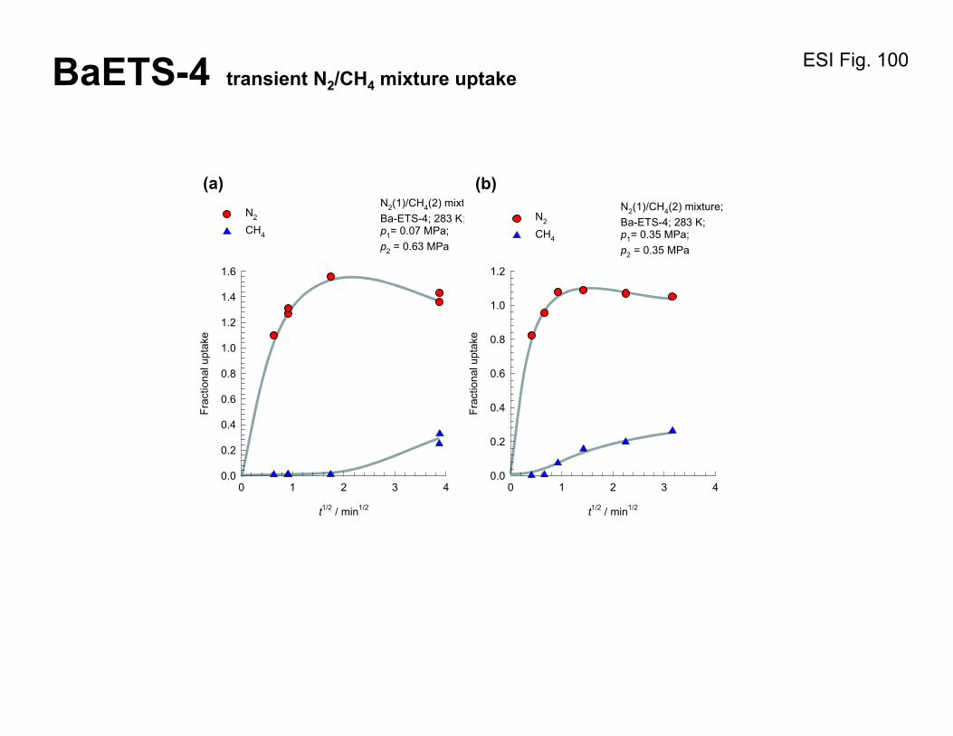
ESI Fig. 100

t1/2 / min1/2

0 1 2 3 4

Frac

tiona

l upt

ake

0.0

0.2

0.4

0.6

0.8

1.0

1.2

1.4

1.6

N2

CH4

N2(1)/CH4(2) mixture;Ba-ETS-4; 283 K;p1= 0.07 MPa;p2 = 0.63 MPa

(a) (b)

t1/2 / min1/2

0 1 2 3 4Fr

actio

nal u

ptak

e0.0

0.2

0.4

0.6

0.8

1.0

1.2

N2

CH4

N2(1)/CH4(2) mixture;Ba-ETS-4; 283 K;p1= 0.35 MPa;p2 = 0.35 MPa

BaETS-4 transient N2/CH4 mixture uptake

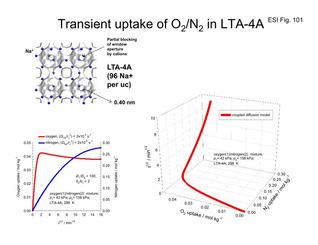
ESI Fig. 101

0

2

4

6

8

10

0.00

0.05

0.100.15

0.200.25

0.30

0.000.01

0.020.03

0.04

t1/2 /

min

1/2

N 2 up

take /

mol

kg-1

O2 uptake / mol kg -1

coupled diffusion model

oxygen(1)/nitrogen(2) mixture;p1= 42 kPa; p2= 158 kPa;LTA-4A; 298 K

Transient uptake of O2/N2 in LTA-4A

t1/2 / min1/2

0 2 4 6 8 10 12 14 16

Oxy

gen

upta

ke /

mol

kg-1

0.00

0.01

0.02

0.03

0.04

0.05

Nitr

ogen

upt

ake

/ mol

kg-1

0.00

0.05

0.10

0.15

0.20

0.25

0.30

oxygen, (DO2/rc2) = 2x10-3 s-1

nitrogen, (DN2/rc2) = 2x10-5 s-1

oxygen(1)/nitrogen(2) mixture;p1= 42 kPa; p2= 158 kPa;LTA-4A; 298 K

Ð1/Ð2 = 100;b2/b1 = 2

0.40 nm

Na+

LTA-4A (96 Na+ per uc)

Partial blocking of window apertureby cations

ESI Fig. 102

N2 uptake / mol kg-1

0.0 0.1 0.2 0.3 0.4 0.5

O2 u

ptak

e / m

ol k

g-1

0.00

0.05

0.10

0.15

0.20

0.25

Chen expt dataadsorption cycledesorption cycle

oxygen(1)/nitrogen(2) mixture; Chen expt dataCMS; 300 K;

Transient uptake of O2/N2 in CMS

(b)(a)

Ð1/Ð2 = 100;b2/b1 = 2

t1/2 / min1/2

0 2 4 6 8

com

pone

nt u

ptak

e / m

ol k

g-1

0.00

0.05

0.10

0.15

0.20

0.25

0.30O2

N2

oxygen(1)/nitrogen(2) mixture; Chen expt dataCMS; 300 K;pO2 = 109.6 kPa;pN2 = 432.56 kPa;

O O

4.3 Å

3.1

Å N N4.4 Å

3.3

Å

ESI Fig. 103

t1/2 / min1/2

0 2 4 6 8 10

Frac

tiona

l app

roac

h to

equ

ilibr

ium

0.0

0.2

0.4

0.6

0.8

1.0

1.2 CH4

C2H6

LTA-4A;Carlson & Dranoff, 1985

Na+

LTA-4A (96 Na+)

Transient uptake CH4/C2H6 in LTA-4A

ESI Fig. 104

ZIF-8 Flexible windows 3.26 Å

propene1.34 Å

1.54 Å

115.5o

123.9o

propane t1/2 / min1/2

0 1 2 3 4 5 6

Com

pone

nt lo

adin

g / m

ol k

g-1

0.0

0.5

1.0

1.5

2.0

2.5

3.0

propene, with thermo couplingpropane, with thermo couplingpropene, with Γij= δij

propane, with Γij= δij

Ð1/Ð2 = 125;b2/b1 = 1.07

ZIF-8; 303 K;ppropene= ppropane = 50 kPa

Propene/propane uptake in ZIF-8

ESI Fig. 105

propene1.34 Å

1.54 Å

115.5o

123.9o

propanet1/2 / min1/2

0 50 100 150 200 250

Com

pone

nt lo

adin

g / m

ol k

g-1

0.0

0.5

1.0

1.5

propene, with thermo couplingpropane, with thermo couplingpropene, with Γij= δij

propane, with Γij= δij

CHA; 353 K;ppropene= ppropane = 50 kPa

Ð1/Ð2 = 5000;b2/b1 = 2.67

CHA

Propene/propane uptake in CHA

ESI Fig. 106

(a) (b)

SAPO-34: Transient uptake of 1-alcohols

t1/2 / h1/2

0.1 1 10

Com

pone

nt u

ptak

e / m

ol k

g-1

0

1

2

3

ethanol in mixture1-propanol in mixture

SAPO-34; 298 K;ethanol/1-propanol;Saint-Remi experiments

t1/2 / h1/2

0 2 4 6 8 10 12 14

Met

hano

l upt

ake

/ mol

kg-1

0.0

0.5

1.0

1.5

2.0

2.5

3.0

3.5

4.0

4.5

1-pr

opan

ol u

ptak

e / m

ol k

g-1

0.0

0.2

0.4

0.6

0.8

1.0

1.2

1.4

methanol1-propanol

SAPO-34; 298 K;methanol/1-propanol

ethanol

Θi,sat= 4/cage

1-propanol

Θi,sat= 2/cage

methanol

Θi,sat= 5.4/cage

ESI Fig. 107

0.0

0.2

0.4

0.6

0.8

1.0

0.00.2

0.40.6

0.81.0

1.21.4

01

23

45

Dim

ensi

onle

ss ra

dial

dis

tanc

e, r/

r c

1-pr

opan

ol loa

ding/

mol kg

-1

ethanol loading / mol kg -1

102 s103 s104 s5x104 s

CHA; 300 K;ethanol(1)/1-propanol(2)

Spherical crystal

r = rc

r = 0

Surface loading

Radial profiles for ethanol/1-propanol transient uptake in CHA

ESI Fig. 108

Eluted volume / mL

0 10 20 30 40 50 60

Dim

ensi

onle

ss c

once

ntra

tion

at o

utle

t, c i /

ci0

0.0

0.2

0.4

0.6

0.8

1.0

1.2

ethanol1-propanol

SAPO-34; 298 K;ethanol(1)/1-propanol(2)Remy et al. expt

t1/2 / h1/2

0.1 1 10

Com

pone

nt u

ptak

e / m

ol k

g-1

0

1

2

3

ethanol in mixture1-propanol in mixture

SAPO-34; 298 K;ethanol/1-propanol;Saint-Remi experiments

ethanol/1-propanolmixture Exit

1-propanolethanol

1-propanol

ethanol

SAPO-34: Transient uptake, and breakthrough

1-propanol

ethanol

(a) (b)

ESI Fig. 109Adsorption/Desorption 1-alcohols in CHA

1-proponal uptake / mol kg-1

1.0 1.2 1.4 1.6 1.8 2.0 2.2 2.4 2.6

etha

nol u

ptak

e / m

ol k

g-1

0

1

2

3

adsorption cycledesorption cycle

pt = 2 kPa to 2 MPa

CHA; 300 K;ethanol(1)/1-propanol(2)

pt = 2 MPa to 2 kPa

t1/2 / h1/2

0.1 1 10

Com

pone

nt u

ptak

e / m

ol k

g-1

0

1

2

3

ethanol1-propanol

CHA; 300 K;ethanol(1)/1-propanol(2)f10 = 1 kPa; f20= 1 kPa;f1 = 1 MPa; f2= 1 MPa;

t1/2 / h1/2

0.1 1 10

Com

pone

nt u

ptak

e / m

ol k

g-1

0

1

2

3

ethanol1-propanol

CHA; 300 K;ethanol(1)/1-propanol(2)f10 = 1 MPa; f20= 1 MPa;f1 = 1 kPa; f2= 1 kPa;

(a) (b)

(c)

1-propanol

Θi,sat= 2/cage

ethanol

Θi,sat= 4/cage

ESI Fig. 110

NaXzeolite

Transient n-heptane/benzene uptake in NaX

Kärger

t 1/2 / min1/2

0 2 4 6 8 10 12 14 16 18

Com

pone

nt lo

adin

g / m

ol k

g-1

0.0

0.2

0.4

0.6

0.8

1.0

1.2

1.4

1.6 n-heptanebenzene

NaX; 359 K;Kärger-Bülow, 1975

ESI Fig. 111

ethylbenzene

benzene

t1/2 / min1/2

0.0 0.5 1.0 1.5 2.0 2.5

Com

pone

nt lo

adin

g / m

ol k

g-1

0.0

0.1

0.2

0.3

0.4

BenzeneEthylBenzene

Benzene(1)/EthylBenzene(2) mixture;H-ZSM-5; 375 K;p1= 115 Pa;p2 = 115 Pa

MFI: Transient uptake of benzene/ethylbenzene mixture

0.0

0.5

1.0

1.5

2.0

2.5

0.0

0.1

0.2

0.3

0.40.5

0.000.02

0.040.06

t1/2 /

min

1/2

ethylb

enze

ne up

take /

mol

kg-1

benzene uptake / mol kg -1

Karge & Niessen data

Benzene(1)/EthylBenzene(2) mixture;H-ZSM-5; 375 K;p1= 115 Pa;p2 = 115 Pa

ESI Fig. 112

0.0

0.2

0.4

0.6

0.8

1.0

1.2

0.000.05

0.100.15

0.200.25

0.300.35

0.000.02

0.040.06

0.08

t1/2 /

min

1/2

p-xy

lene u

ptake

/ mol

kg-1

benzene uptake / mol kg -1

Karge & Niessen data

Benzene(1)/p-Xylene(2) mixture;H-ZSM-5; 395 K;p1= 115 Pa;p2 = 115 Pa

t1/2 / min1/2

0.0 0.5 1.0 1.5

Com

pone

nt lo

adin

g / m

ol k

g-1

0.0

0.1

0.2

0.3

Benzenep-Xylene

Benzene(1)/p-Xylene(2) mixture;H-ZSM-5; 395 K;p1= 115 Pa;p2 = 115 Pa

MFI: Transient uptake of benzene/p-xylene mixtures

benzenep-xylene

ESI Fig. 113

0.0

0.5

1.0

1.5

2.0

2.5

3.0

0.0

0.5

1.0

1.52.0

01

23

t1/2 /m

in1/

2

2MP uptake / molecules per unit c

ell

nC6 uptake / molecules per unit cell

Titze expt datauncoupled diffusion

nC6/2MP mixture; MFI; T = 298 K;p1=p2 = 0 Pa to 1.3 Pa;

Total loading, Θt / molecules per unit cell

0 1 2 3 4 5 6 7 8

( Γ12

Θ2/

Γ 11Θ

1)

0.00

0.05

0.10

0.15

0.20

0.25

0.30

(Γ12Θ2/ Γ11Θ1)

nC6-2MP mixture; p1=p2;Calculations from simplifiedmixed gas Langmuir;300 K; MFI

t1/2 / min1/2

0 1 2 3 4 5

Upt

ake

/ mol

ecul

es p

er u

nit c

ell

0.0

0.5

1.0

1.5

2.0

2.5

3.0

3.5nC6, M-S model2MP, M-S model

nC6/2MP mixture; MFI; T = 298 K;p1=p2 = 0 Pa to 1.3 Pa;M-S model without thermodynamic coupling

t1/2 / min1/2

0 1 2 3 4 5

Upt

ake

/ mol

ecul

es p

er u

nit c

ell

0.0

0.5

1.0

1.5

2.0

2.5

3.0

3.5

nC6, IRM2MP, IRMnC6, M-S model2MP, M-S model

nC6 diffusivity:Ð1 / rc

2 = 0.016 s-1

2MP diffusivity:Ð2 / rc

2 = 1.6 x 10-4 s-1

nC6/2MP mixture; MFI; T = 298 K;p1=p2 = 0 Pa to 1.3 Pa

(c)

(a)

MFI transient nC6/2MP mixture uptake

(b)

ESI Fig. 114

0.0

0.2

0.4

0.6

0.8

1.0

0.0

0.5

1.0

1.5

2.0

01

23

Dim

ensi

onle

ss ra

dial

dis

tanc

e, r/

r c

2MP

loadin

g / m

olecu

les/uc

nC6 uptake / molecules/uc

t = 5 st = 10.2 st = 50.6 st = 832 s

nC6/2MP mixture; MFI; T = 298 K;p1=p2 = 0 Pa to 1.3 Pa;

Spherical crystal

r = rc

r = 0

Surface loading

Radial profiles for transient nC6/2MP mixture uptake in MFI

ESI Fig. 115

0

1

2

3

4

5

6

0.0

0.5

1.01.5

2.0

0.00.5

1.01.5

2.02.5

3.0

t1/2 /m

in1/

2

2MP uptake / molecules uc

-1

nC6 uptake / molecules uc -1

AdsorptionDesorptionuncoupled

p1=p2 =1.3 Pa to 0 Pa;

p1=p2 =0 Pa to 1.3 Pa;

nC6(1)/2MP(2) mixture; MFI; T = 298 K

(a)

2MP loading / molecules uc-1

0.0 0.5 1.0 1.5 2.0

nC6

load

ing

/ mol

ecul

es u

c-1

0.0

0.5

1.0

1.5

2.0

2.5

3.0

3.5

adsorption phasedesorption phaseuncoupled p1=p2 =

0 Pa to 1.3 Pa;

p1=p2 =1.3 Pa to 0 Pa;

nC6(1)/2MP(2) mixture; MFI; T = 298 K

(b)

Adsorption-Desorption Asymmetry

2MPnC6

stra

ight

cha

nnel

s

ESI Fig. 116

nC6/2MP mixture; MFI; T = 298 K;p1=p2 = 0 Pa to 1.3 Pa;

0.0

0.5

1.0

1.5

2.0

2.5

1.31.4

1.51.6

1.7

1.52.0

2.53.0

t1/2 /m

in1/

2

2MP uptake / molecules per unit cell

nC6 uptake / molecules per unit cell

adsorption cycledesorption cycleuncoupled

nC6(1)/2MP(2) mixture; MFI; T = 298 K

p1=p2 = 2 Pa to 0 .2 Pa

p1=p2 =0.2 Pa to 2 Pa;

undershoot

overshoot

2MP loading / molecules uc-1

1.3 1.4 1.5 1.6 1.7 1.8

nC6

load

ing

/ mol

ecul

es u

c-1

1.5

2.0

2.5

3.0

adsorption cycledesorption cycleuncoupled

p1=p2 =0.2 Pa to 2 Pa;

p1=p2 = 2 Pa to 0 .2 Pa

nC6(1)/2MP(2) mixture; MFI; T = 298 K

undershoot

overshoot

(a)Undershoots and Overshoots

(b)

ESI Fig. 117

0.0

0.2

0.4

0.6

0.8

1.0

0.00.20.40.60.81.01.21.4

01

23

4

t1/2 /m

in1/

2

iC4 uptake / molecules per unit cell

nC4 uptake / molecules per unit cell

adsorption cycledesorption cycleuncouplednC4(1)/iC4(2) mixture;

MFI; T = 298 K

p1=p2 =100 Pa to 0 Pa;

p1=p2 =0 Pa to 100 Pa;

nC4/iC4 adsorption-desorption asymmetry(a)

(b)

iC4 loading / molecules uc-1

0.0 0.5 1.0 1.5

nC4

load

ing

/ mol

ecul

es u

c-1

0

1

2

3

4

adsorption cycledesorption cycleuncoupled

nC4(1)/iC4(2) mixture; MFI; T = 298 K

p1=p2 =0 Pa to 100 Pa;

p1=p2 =100 Pa to 0 Pa;

ESI Fig. 118

benzene loading / mol kg-1

0.0 0.1 0.2

p- x

ylen

e lo

adin

g / m

ol k

g-1

0.0

0.1

0.2

0.3

p-xylene adsorption:p2 = 0 Pa to 115 Pap-xylene desorption:p2 = 115 Pa to 0 Pa

Niessen & Kargeexperiment;Benzene(1)/p-Xylene(2) mixture;H-ZSM-5; 395 K

t1/2 / min1/2

0 1 2 3 4 5

Com

pone

nt lo

adin

g / m

ol k

g-1

0.0

0.1

0.2

0.3

p-xylene adsorption:p2 = 0 Pa to 115 Pap-xylene desorption:p2 = 115 Pa to 0 Pabenzene:p1 = 115 Pabenzene:p1 = 115 Pa

Niessen & Kargeexperiment;Benzene(1)/p-Xylene(2) mixture;H-ZSM-5; 395 K

benzene

(a)

p-xylene

MFI: Transient adsorption/desorption benzene/p-xylene mixtures

(b)

ESI Fig. 119

nC6/2MP mixture; MFI; T = 298 K;p1=p2 = 0 Pa to 1.3 Pa;

0

1

2

3

4

5

6

01

23

01

23

45

t1/2 /m

in1/

2

2MP uptake / molecules per unit cell

nC6 uptake / molecules per unit cell

adsorb nC6, desorb 2MPdesorb nC6, adsorb 2MPuncoupled

p1 = 0 Pa to 1.3 Pap2= 1.3 Pa to 0 Pa

p1= 1.3 Pa to 0 Pap2 = 0 Pa to 1.3 Pa

nC6(1)/2MP(2) mixture; MFI; T = 298 K

2MP loading / molecules uc-1

0 1 2 3

nC6

load

ing

/ mol

ecul

es u

c-1

0

1

2

3

4

adsorp nC6, desorp 2MPdesorb nC6, adsorp 2MPuncoupled

nC6(1)/2MP(2) mixture; MFI; T = 298 K

p1= 1.3 Pa to 0 Pap2 = 0 Pa to 1.3 Pa

p1 = 0 Pa to 1.3 Pap2= 1.3 Pa to 0 Pa

(b)

(a)Counter-current uptake

2MPnC6

stra

ight

cha

nnel

s

ESI Fig. 120

t1/2 / min1/2

0 1 2 3 4 5

Com

pone

nt lo

adin

g, q

i / m

ol k

g-1

0.0

0.1

0.2

0.3

23DMB22DMB3MP2MPnC6

(DnC6/rc2) = 0.002 s-1;

(DnC6/D2MP) = 5(DnC6/D3MP) = 5(DnC6/D22DMB) = 25(DnC6/D23DMB) = 25

Including diffusion;but ignoring thermo coupling

(a) (b)

Transient uptake of hexane isomers in MFI crystal

t1/2 / min1/2

0 1 2 3 4 5

Com

pone

nt lo

adin

g, q

i / m

ol k

g-1

0.0

0.1

0.2

0.3

0.4

0.5

23DMB22DMB3MP2MPnC6

(DnC6/rc2) = 0.002 s-1;

(DnC6/D2MP) = 5(DnC6/D3MP) = 5(DnC6/D22DMB) = 25(DnC6/D23DMB) = 25

Including diffusion;includingthermocoupling

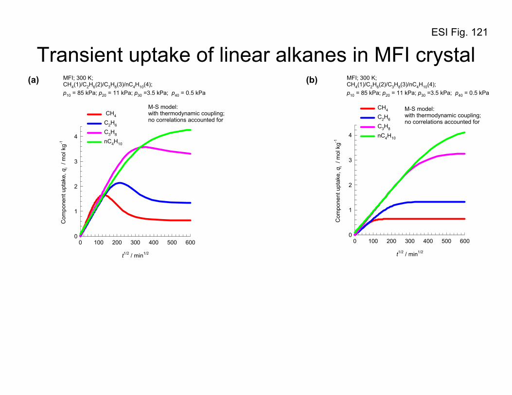
ESI Fig. 121

t1/2 / min1/2

0 100 200 300 400 500 600

Com

pone

nt u

ptak

e, q

i / m

ol k

g-1

0

1

2

3

4

CH4

C2H6

C3H8

nC4H10

M-S model:with thermodynamic coupling;no correlations accounted for

MFI; 300 K; CH4(1)/C2H6(2)/C3H8(3)/nC4H10(4);p10 = 85 kPa; p20 = 11 kPa; p30 =3.5 kPa; p40 = 0.5 kPa

(a) (b)

Transient uptake of linear alkanes in MFI crystal

t1/2 / min1/2

0 100 200 300 400 500 600

Com

pone

nt u

ptak

e, q

i / m

ol k

g-1

0

1

2

3

4

CH4

C2H6

C3H8

nC4H10

M-S model:with thermodynamic coupling;no correlations accounted for

MFI; 300 K; CH4(1)/C2H6(2)/C3H8(3)/nC4H10(4);p10 = 85 kPa; p20 = 11 kPa; p30 =3.5 kPa; p40 = 0.5 kPa

ESI Fig. 122Propene/propane permeation

ZIF-8Flexible windows 3.3 Å

1.34 Å

123.9o

1.54 Å

115.5o

propane

propene

propane

propene

t1/2 / min1/2

0 1 2 3 4 5

Flux

of p

rope

ne /

10-3

mol

m-2

s-1

0.0

0.2

0.4

0.6

0.8

1.0

1.2

1.4

Flux

of p

ropa

ne /

10-5

mol

m-2

s-1

0.0

0.2

0.4

0.6

0.8

1.0

1.2

1.4propenepropane

ZIF-8; 303 K;ppropene= ppropane

= 50 kPa

Ð1/Ð2 = 125;b2/b1 = 1.07

t1/2 / min1/2

0 1 2 3 4 5

Flux

of p

rope

ne /

10-3

mol

m-2

s-1

0.0

0.2

0.4

0.6

0.8

1.0

1.2

1.4

Flux

of p

ropa

ne /

10-5

mol

m-2

s-1

0.0

0.2

0.4

0.6

0.8

1.0

1.2

1.4

propenepropane

ZIF-8; 303 K;ppropene= ppropane

= 50 kPa

Ð1/Ð2 = 125;b2/b1 = 1.07

(a) (b)

ESI Fig. 123

CH4/n-C4H10 permeation: MFI membrane

MFI membranet1/2 / min1/2

0.7 0.8 0.9 1.0 1.1 1.2

Cco

mpo

nent

flux

es, N

i / m

mol

m-2

s -2

0

1

2

3

4

methanen-butane

MFI membrane; 298K; CH4(1)/nC4H10(2) equimolar gas mixture

ESI Fig. 124MFI transient permeation of linear alkanes

(a) (b)

t1/2 / min1/2

0 1 2 3

Com

pone

nt fl

uxes

, Ni

/ mm

ol m

-2 s

-1

0

5

10

15

20

25

CH4

C2H6

C3H8

nC4H10

M-S model:with thermodynamic coupling;no correlations accounted for

MFI; 300 K; CH4(1)/C2H6(2)/C3H8(3)/nC4H10(4);p10 = p20 = p30 =30 kPa; p40 = 10 kPa

t1/2 / min1/2

0 1 2 3 4

Com

pone

nt fl

uxes

, Ni

/ mm

ol m

-2 s

-1

0

1

2

3

4CH4

C2H6

C3H8

nC4H10

M-S model:no thermodynamic coupling;no correlations accounted for

MFI; 300 K; CH4(1)/C2H6(2)/C3H8(3)/nC4H10(4);p10 = p20 = p30 =30 kPa; p40 = 10 kPa

MFI membrane

ESI Fig. 125MFI H2/n-C4H10 transient mixture permeation

MFI membranetime / s

0 50 100 150

Flux

/ m

mol

m-2

s-1

0.0

0.5

1.0

1.5

2.0

2.5 MFI; 295 K; H2/nC4 mixture;pH2= 95 kPa;pnC4 = 5 kPa;Expt dataBakker

nC4

H2

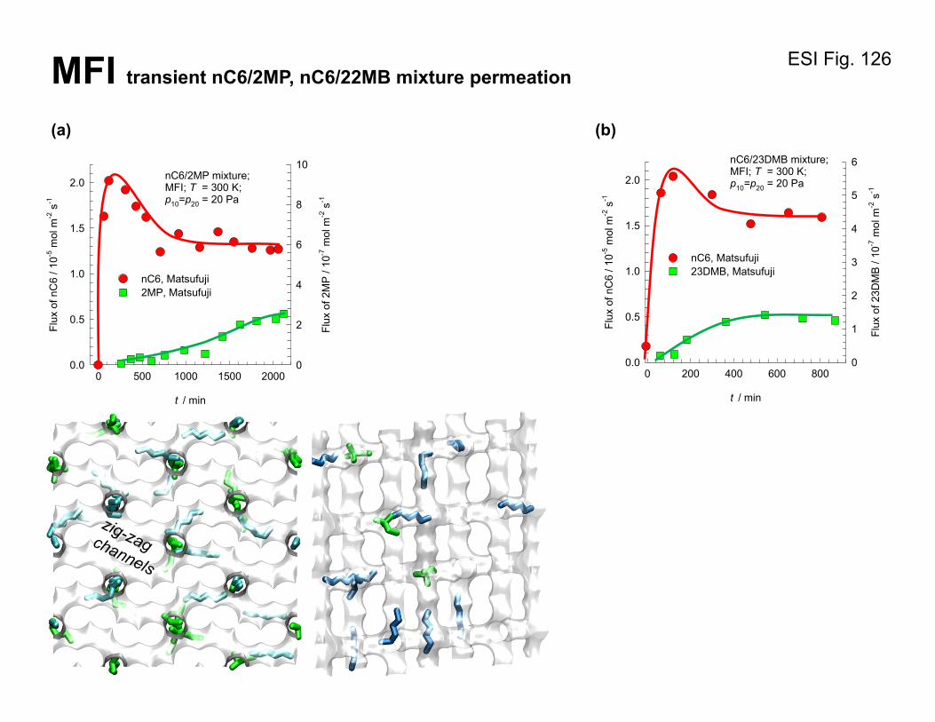
ESI Fig. 126

t / min

0 200 400 600 800

Flux

of n

C6

/ 10-5

mol

m-2

s-1

0.0

0.5

1.0

1.5

2.0

Flux

of 2

3DM

B /

10-7

mol

m-2

s-1

0

1

2

3

4

5

6

nC6, Matsufuji23DMB, Matsufuji

nC6/23DMB mixture; MFI; T = 300 K;p10=p20 = 20 Pa

t / min

0 500 1000 1500 2000

Flux

of n

C6

/ 10-5

mol

m-2

s-1

0.0

0.5

1.0

1.5

2.0

Flux

of 2

MP

/ 10

-7 m

ol m

-2 s

-1

0

2

4

6

8

10

nC6, Matsufuji2MP, Matsufuji

nC6/2MP mixture; MFI; T = 300 K;p10=p20 = 20 Pa

(a) (b)

MFI transient nC6/2MP, nC6/22MB mixture permeation

ESI Fig. 127

t / min

0 5 10 15 20 25

Flux

/ 10

-7 m

ol m

-2 s

-1

0.0

0.5

1.0

1.5

2.0

2.5

3.0

3.5p-xylenem-xylene

50/50 p-xylene/m-xylenemixture; MFI; T = 303 K

(a) (b)

t / min

0 5 10 15 20 25 30

Flux

/ 10

-7 m

ol m

-2 s

-1

0.0

0.5

1.0

1.5

2.0

2.5

3.0

p-xylenem-xyleneo-xylene

24/51/25 p-xylene/m-xylene/o-xylenemixture; MFI; T = 303 K

m-xylene is preferentially located at the intersections of MFI

p-xylene can locate along the channels MFI

o-xylene is preferentially located at the intersections of MFI

MFI transient xylene isomers mixture permeation

ESI Fig. 128

time, t / s

0 1000 2000 3000 4000

Com

pone

nt fl

uxes

/ 10

-5 m

ol m

-2- s

-1

0.0

0.2

0.4

0.6

0.8

1.0

1.2

1.4

1.6p-xylenebenzene

benzene/p-xylene mixture; MFI; T =313 K;p10 = 578.7 Pap20 = 322.9 Pa

MFI transient benzene/p-xylene mixture permeation

time, t / s

0 1000 2000 3000 4000

Com

pone

nt fl

uxes

/ 10

-5 m

ol m

-2- s

-1

0.0

0.2

0.4

0.6

0.8

1.0

1.2

1.4 p-xylenebenzene

benzene/p-xylene mixture; MFI; T =343 K;p10 = 578.7 Pap20 = 322.9 Pa

time, t / s

0 200 400 600 800 1000

Com

pone

nt fl

uxes

/ 10

-5 m

ol m

-2- s

-1

0.0

0.5

1.0

1.5

2.0

2.5p-xylenebenzene

benzene/p-xylene mixture; MFI; T = 403 K;p10 = 578.7 Pap20 = 322.9 Pa

(a) (b) (c)

benzenep-xylene