Blind separation of convolutive mixtures of cyclostationary signals

INTERNATIONAL JOURNAL OF ADAPTIVE CONTROL AND SIGNAL PROCESSINGInt. J. Adapt. Control Signal Process. 2004; 18:279–298 (DOI: 10.1002/acs.794)

Blind separation of convolutive mixtures ofcyclostationary signals

Wenwu Wangn,w, Maria G. Jafari, Saeid Sanei and Jonathon A. Chambers

Centre for Digital Signal Processing Research, Department of Electronic Engineering, King’s College London,

London WC2R 2LS, U.K.

SUMMARY

An adaptive blind source separation algorithm for the separation of convolutive mixtures ofcyclostationary signals is proposed. The algorithm is derived by applying natural gradient iterativelearning to a novel cost function which is defined according to the wide sense cyclostationarity of signalsand can be deemed as a new member of the family of natural gradient algorithms for convolutive mixtures.A method based on estimating the cycle frequencies required for practical implementation of the proposedalgorithm is presented. The efficiency of the algorithm is supported by simulations, which show that theproposed algorithm has improved performance for the separation of convolved cyclostationary signals interms of convergence speed and waveform similarity measurement, as compared to the conventionalnatural gradient algorithm for convolutive mixtures. Copyright # 2004 John Wiley & Sons, Ltd.

KEY WORDS: blind source separation (BSS); convolutive mixtures; cyclostationary signals; naturalgradient learning; cycle frequency determination

1. INTRODUCTION

In many practical situations such as in the radiocommunications, telemetry, radar, sonar andspeech contexts, the sources are non-stationary and very often (quasi)-cyclostationary and theobserved signals are usually convolutive mixtures, so that the conventional methods for thestandard blind source separation (BSS) problem, in which the mixtures are assumed to beinstantaneous and the source signals are assumed to be statistically stationary [1], are no longerappropriate. Increasing interest has therefore been focused on solving the problem of BSS ofconvolutive mixtures and the main existing strategies can be approximately classified into [2]: (1)carrying out blind separation in the time domain by extending the existing BSS algorithms forthe instantaneous case to the convolutive case [3]; (2) transforming totally or partially the

Contract/grant sponsor: Engineering and Physical Sciences Research Council, U.K.

Published online 2 March 2004 Revised 10 March 2003Accepted 17 October 2003Copyright # 2004 John Wiley & Sons, Ltd.

wE-mail: [email protected]

nCorrespondence to: Dr. Wenwu Wang, Department of Electronic Engineering, King’s College London, Strand,London WC2R 2LS, U.K.

convolutive BSS problem into multiple instantaneous problems in the frequency domain andseparating the instantaneous mixtures in every frequency bin [4, 5]; (3) decomposing the problemrather than learning the possibly huge filters all at once, i.e. the decorrelation approach,subspace method, or subband decomposition approach [6]; (4) exploiting the statisticalproperties or special structure contained within the source signals to formulate variousseparation criteria [7].

Addressing the BSS problem for cyclostationary sources is a relatively new approach. Meraimet al. [7] proposed to minimize a cost function constructed from the cyclic cross-correlation ofrecovered sources at various time lags, and they presented iterative update equations followingfrom the natural gradient technique. Ferreol and Chevalier [8] have shown that the currentsecond- or higher-order BSS methods perform poorly if the assumption that the source signalsare statistically stationary remains unchanged. Most existing BSS approaches exploiting thecyclostationarity of the sources are either batch algorithms as in Reference [8] or are based onsecond-order statistics as in Reference [7], and very few of them are concerned with theconvolutive mixtures. In this paper, we propose a sequential BSS algorithm for convolutivemixtures using high-order conventional statistics and second-order cyclostationarity of thesource signals. We will show that the statistical property of cyclostationary signals can beexploited to increase the separability (or separation quality) of the convolutive mixtures ofcyclostationary sources. The ensuing sections are organized as follows. The data model isformulated in Section 2 and the proposed algorithm for instantaneous mixtures and convolutivemixtures is detailed in Section 3 which also includes the analysis of the stability condition of thealgorithm. A proposed estimation method for the cycle frequencies which are required for theproposed algorithm is presented in Section 4. The simulation results and conclusions are,respectively, presented in Sections 5 and 6. The derivation of several equations in Section 3 isattached in Section 7 (i.e. the appendix).

2. PROBLEM FORMULATION

Assume that N source signals are recorded by M sensors, where M5N : The output of eachsensor is modelled as a weighted sum of convolutions of the source signals corrupted by additivenoise. In a compact form, we have

xðkÞ ¼ HðzÞsðkÞ þ vðkÞ ð1Þ

where sðkÞ 2 CN is the source vector, xðkÞ 2 C

N is the sensor vector, k is the discrete time index;HðzÞ is the z-transform of the mixing matrix with entries HijðzÞ ¼

PP�1p¼0 hijpz�p ði ¼ 1; . . . ;M ;

j ¼ 1; . . . ;N Þ; where z�1 is the time-shift operator, i.e. z�1sjðkÞ ¼ sjðk � 1Þ: For simplicity, weignore additive noise in the following derivations. The source signal vector sðkÞ is modelled as awide sense cyclostationary signal [9], and its components siðkÞ are assumed to be mutuallyindependent with zero mean.

The aim is to reconstruct the source signals siðkÞ (up to an arbitrary permutation and filteringoperation) from only knowledge of the sensor signals xiðkÞ without knowing the source signalsand the mixing process. Alternatively, we have

yðkÞ ¼ Wðz; kÞxðkÞ ð2Þ

¼ Wðz; kÞHðzÞsðkÞ ¼ Cðz; kÞsðkÞ ð3Þ

Copyright # 2004 John Wiley & Sons, Ltd. Int. J. Adapt. Control Signal Process. 2004; 18:279–298

WENWU WANG ET AL.280

where yðkÞ 2 CN is the output vector of estimated source signals with entries yiðkÞ ¼

PNj¼1

Wijðz; kÞxjðkÞ; Wðz; kÞ is the unmixing temporal network with entries Wijðz; kÞ ¼PL

p¼0 wijpðkÞz�p:

The task is to adjust Wðz; kÞ such that limk!1 Cðz; kÞ ¼ PKDðzÞ; where P 2 RN�N is apermutation matrix, K 2 RN�N is a non-singular diagonal scaling matrix, and DðzÞ is a diagonalmatrix whose iith entry is

Pp cipz�p; cip is a complex scalar weighting, and p is an integer delay

value. This formulation makes the i.i.d. assumption in the deconvolution context unnecessaryfor convolutive BSS. Taking advantage of the scale and permutation indeterminacy of theconventional BSS methods [9], we assume that the cyclic correlation matrix of the sources at lagt ¼ 0 follows Rbi

s ðkÞ½0� ¼ EfeJbiksðkÞsHðkÞg ¼ I0i; where ð�ÞH denotes the Hermitian transposeoperator, I0i has entries as follows:

½I0i�l;g ¼1 if l 2 f1; 2; . . . ;Ng; g ¼ l ¼ i

0 otherwise

(ð4Þ

3. THE PROPOSED ALGORITHM

3.1. Separation of instantaneous mixtures of cyclostationary sources

The wide sense cyclostationarity assumption implies that the cyclic correlation function of thesources satisfies [7]:

heJbiksiðk þ tÞsnj ðkÞi ¼ 0 if i=j ð5Þ

heJbjksiðk þ tÞsni ðkÞi ¼ 0 if bi=bj ð6Þ

heJbiksiðkÞsni ðkÞi > 0 8i ð7Þ

where J ¼ffiffiffiffiffiffiffi�1

p; the superscript * denotes complex conjugation, h�i denotes the time averaging

operator, and bi is a non-zero cycle frequency of source i: It is worth noting that we use h�i andEð�Þ to denote time-averages for discrete- and continuous-time operations, respectively, as thecontext demands [10]. The equivalence has been shown in Reference [8]. Invoking theseproperties into the Kullback–Leibler divergence criterion, our cost function is defined as (seeReferences [9, 11])

rðWðkÞÞ ¼ � log detðWðkÞÞ �XNi¼1

log piðyiðkÞÞ

þ1

2fTrð *RRb

yðkÞÞ � log detð *RRbyðkÞÞ � Ng ð8Þ

where Trð�Þ and detð�Þ are, respectively, the trace and determinant operators, and piðyiðkÞÞis an appropriately chosen probability density function (pdf) of yðkÞ which is derived from thepast sequence of xðkÞ by the separation matrix WðkÞ: The term *RRb

yðkÞ is defined as

*RRbyðkÞ ¼

XNi¼1

Rbiy ðkÞ ð9Þ


BLIND SEPARATION 281

where Rbiy ðkÞ ¼ heJbikyðkÞyTðkÞi is the output cyclic correlation matrix for the ith cycle frequency

which is required to satisfy limk!1 Rbiy ðkÞ ¼ I0i; where the elements of I0i take the form in (4) and

time lag in Rbiy ðkÞ is omitted for simplicity. At convergence,

limk!1

*RRbyðkÞ ¼ I ð10Þ

Iterative learning can be used to minimize the cost function in (8). Applying the natural gradientrule [12] together with a cyclic decorrelation operation, we obtain a new learning rule as (see theappendix)

Wðk þ 1Þ ¼WðkÞ þ mðkÞ½I� fðyðkÞÞyTðkÞ

þ I� *RRbyðkÞ�WðkÞ ð11Þ

where mðkÞ is the learning rate and fð�Þ is a vector of non-linear activation functions.For simplicity, we call the algorithm in (11) the CSNGA algorithm corresponding to thenatural gradient algorithm (NGA). Observing the learning rule in (11), we see that theproposed algorithm has a similar form to the equivariant adaptive algorithm proposed byCardoso and Laheld [13] and equivariant non-stationary algorithm proposed by Choi et al. [14].More specifically, comparing the term I� *RRb

yðkÞ in (11) and its counterpart in References[13, 14], it is clear that rather than incorporating the cyclostationary statistics as in (11), awhitening process with the form of I� yyT was directly incorporated in the learning processin Reference [13], and a form of I�P�1yyT was employed for the non-stationary statisticsin Reference [14], where the elements of the diagonal matrix P can be estimated by thevariance of y:

3.2. Separation of convolutive mixtures of cyclostationary sources

For convolutive BSS, from the algebraic point of view, they have equivalent mathematicalmodels to the instantaneous cases, only being different in the description (IIR filter, FIR filter,Z-transform, wavelets, other transforms) of the physical phenomena [12]. This means, forconvolutive mixtures, the complicated problem can be simplified by applying such transforms.In terms of this fact, it is straightforward to use the Z-transform and define the following costfunction for convolutive mixtures of cyclostationary sources (see Reference [15]):

rðWðz; kÞÞ ¼ rgðWðz; kÞÞ þ rbðWðz; kÞÞ ð12Þ

where rgðWðz; kÞÞ and rbðWðz; kÞÞ are, respectively,

rgðWðz; kÞÞ ¼ �XNi¼1

log piðyiðkÞÞ �1

2pJ

Ilog jdetWðz; kÞjz�1 dz

rbðWðz; kÞÞ ¼ 12fTrð *RRb

yðkÞÞ � log detð *RRbyðkÞÞ � Ng

Here, we assume both HðzÞ and Wðz; kÞ are stable with no zero eigenvalues on the unitcircle jzj ¼ 1: To obtain a learning algorithm which minimizes the cost function (12), wefollow the derivation of the algorithm presented by Amari et al. [12] and calculatethe infinitesimal increment drðWðz; kÞÞ corresponding to an increment dWðz; kÞ: Introducingthe Lie group operation and Riemanian structure on the manifold of FIR filters MðLÞ;dXðz; kÞ ¼ dWðz; kÞ WwðzÞ; where and w are the multiplication and inverse operation defined



in the manifold MðLÞ; drgðWðz; kÞÞ takes the following form by simple algebraic and differentialcalculus [12]:

drgðWðz; kÞÞ ¼ fTðyðkÞÞ dXðz; kÞ½yðkÞ� � TrðdXðz; kÞÞ ð13Þ

Notice that yðkÞ ¼ Wðz; kÞxðkÞ; *RRx ¼ hxðkÞxTðkÞi; and the property dyðkÞ ¼ dXðz; kÞyðkÞ; wehave (see appendix)

dflog detð *RRbyðkÞÞg ¼ d N log

XNi¼1

eJbik

!( )þ dflog det *RRxg þ 2 TrfdWðz; kÞW�1ðz; kÞg ð14Þ

dfTrð *RRbyðkÞÞg ¼ 2

XNi¼1

eJbik

!hyHðkÞ dXðz; kÞyðkÞi ð15Þ

where dXðz; kÞ is denoted asPL

p¼0 dXpðkÞz�p: Notice that d N logPN

i¼1 eJbik� �n o

and dflog det

*RRxg do not depend on the weight matrix Wðz; kÞ; d log det *RRbyðkÞ

� �n ocan be reduced to

2 tr dWðz; kÞW�1ðz; kÞg; therefore we have

drbðWðz; kÞÞ ¼ � TrfdWðz; kÞW�1ðz; kÞg

þXNi¼1

eJbik

!hyTðkÞ dXðz; kÞyðkÞi ð16Þ

From (13) and (16), the partial derivation of rðWðz; kÞÞ with respect to Xðz; kÞ leads to

@rðWðz; kÞÞ@XpðkÞ

¼ ffðyðkÞÞyTðk � pÞ � Idpg

þ �Idp þXNi¼1

heJbikyðkÞyTðk � pÞi

( )ð17Þ

The truncated form of dXðz; kÞ on the FIR filter manifold MðLÞ; i.e. ½dWðz; kÞW�1ðz; kÞ�L; impliesthat the partial derivative of rðWðz; kÞÞ with respect to Wðz; kÞ can be obtained according to thepartial derivative with respect to Xðz; kÞ; this leads to a new learning algorithm for the separationof convolutive mixtures of cyclostationary signals

Wpðk þ 1Þ ¼WpðkÞ þ mðkÞfWpðkÞ � #QQqðkÞ

þ WpðkÞ � fðyðkÞÞuTg ðkÞg ð18Þ

where ugðkÞ ¼PL

q¼0 WTL�qðkÞyðk � p � qÞ; #QQqðkÞ ¼

PLq¼0 WT

L�qðkÞ #RRbyðkÞ½q�; and #RRb

yðkÞ½q�; equiva-lent to the last term in (17), can be estimated by a sample filtering approach, #RRb

yðkÞ½p� ¼ ð1� Z0Þ #RR

byðkÞ½p� þ Z0

PNi¼1 eJbikyðkÞyTðk � pÞ; where Z0 is a forgetting factor. For

simplicity, we call the algorithm in (18) the ConvCSNGA algorithm corresponding to thenatural gradient algorithm for convolutive mixtures (ConvNGA).

The equilibrium points of the proposed learning algorithm satisfy

limk!1

I�XNi¼1

eJbikyðkÞyTðkÞ

* +¼ 0 ð19Þ



limk!1

XNi¼1

eJbikyðkÞyTðk � pÞ

* +¼ 0 ð20Þ

limk!1

hfðyðkÞÞyTðk � pÞi ¼ 0 ð21Þ

limk!1

hI� fðyðkÞÞyTðkÞi ¼ 0 ð22Þ

where p ¼ 1; 2; . . . ;L: This implies that the proposed learning algorithm has a drawback that itforces the output signals to have nearly flat frequency spectra, which however can be mitigatedby following the non-holonomic constraint, that is, using WpðkÞKðkÞ instead of WpðkÞ in (18),where KðkÞ ¼ diagffðyðkÞÞyTðkÞg (see Reference [12] for more details).

In implementation, the infinite system is approximated by the FIR filter given yðkÞ ¼PLp¼0 WpðkÞxðk � pÞ and a similar approximation to the updating equation for the general case

that all signals and coefficients are complex-valued yields

Wpðk þ 1Þ ¼WpðkÞ þ mðkÞfWpðkÞ � #QQpþqðk � LÞ

þ WpðkÞ � fðyðk � LÞÞuHg ðk � pÞg ð23Þ

It is necessary to use split-complex non-linearities in the complex case, e.g. fiðyiðkÞÞ ¼tanhðyiRðkÞÞ þ J tanhðyiIðkÞÞ; where yiRðkÞ and yiIðkÞ are, respectively, the real and imaginaryparts of yiðkÞ; for the sources with super-Gaussian distributions, or fiðyiðkÞÞ ¼ yiðkÞjyiðkÞj2 forthe sub-Gaussian case [9, 13]. In practice, the output cyclic operation term is estimated on-lineusing an exponentially weighted moving average of the statistics with the filtering output data.The algorithm requires approximately 4MN ðN þ 1ÞðLþ 1Þ þ 2N multiplications per timeinstant, and it requires approximately ððM þ 1ÞðN þ 1ÞN þMÞðLþ 1Þ memory locations toimplement. A normalized step size is used in practice mðkÞ ¼ m=frþ

PLp¼0 jyðk � pÞj2g; where r

is a positive value which avoids an explosive growth of step size. Another implementationproblem is the selection of cyclic frequency. The cyclic frequency detection will be discussed inSection 4.

3.3. Stability and convergence analysis of the learning algorithm

To analyse the stability of the learning algorithm (18), we follow the method in References[16, 17] and alternatively consider the continuous-time learning algorithm for updating Xp:

dXp

dt¼ mðdpI� hfðyðtÞÞyTðt � pÞi þ dpI�

XNi¼1

heJbikyðtÞyTðt � pÞiÞ ð24Þ

where p ¼ 0; 1; . . . ;L: By considering expectation in Equation (24), we can examine thebehaviour of the averaged system

dXp

dt¼ mðdpI� EffðyðtÞÞyTðt � pÞg þ dpI�

XNi¼1

EfeJbikyðtÞyTðt � pÞg ð25Þ

Taking a variation dXp of Xp; we have

ddXp

dt¼ �mðEff 0bðyÞdyy

Tðt � pÞ þ fbðyÞdyTðt � pÞg ð26Þ



where fbðyÞ ¼ fðyðtÞÞ þ eJbkyðtÞ and f 0bðyÞ is the derivation of fbðyÞ with respect to y; eJbk ¼4PNi¼1 eJbik ; dyðk � pÞ ¼ ½dXðzÞ�yðk � pÞ ¼

P1j¼0 dXpyðk � p � jÞ: Due to the spatially indepen-

dent assumption of the source signals and the conditions in (19)–(22), if we further suppose thesources are temporally identical and independent, then (26) can be reduced to the followingequation by omitting the last term:

ddXp

dt¼

�mðEff 0bðyÞdXpyðt � pÞyTðt � pÞgÞ; p=0

�mðEff 0bðyÞdX0yyTg þ dX0Þ; p ¼ 0

(ð27Þ

Let *mmi ¼ Eff 0bðyiÞy

2i g; *kki ¼ Eff 0

b;iðyiÞg; and *ss2i ¼ Efjyij2g: The stability conditions for (27) can be

formulated as

*mmi þ 1 > 0 ð28Þ

*kki > 0 ð29Þ

*ss2i *ss2j *kki *kkj > 1 ð30Þ

The conditions are similar to the ones by Zhang et al. [16] for blind source separation of theconvolutive case and by Amari et al. [17] for the instantaneous case, which can be satisfied bychoosing a suitable non-linear activation function plus a linear function with cycle frequencycoefficients.

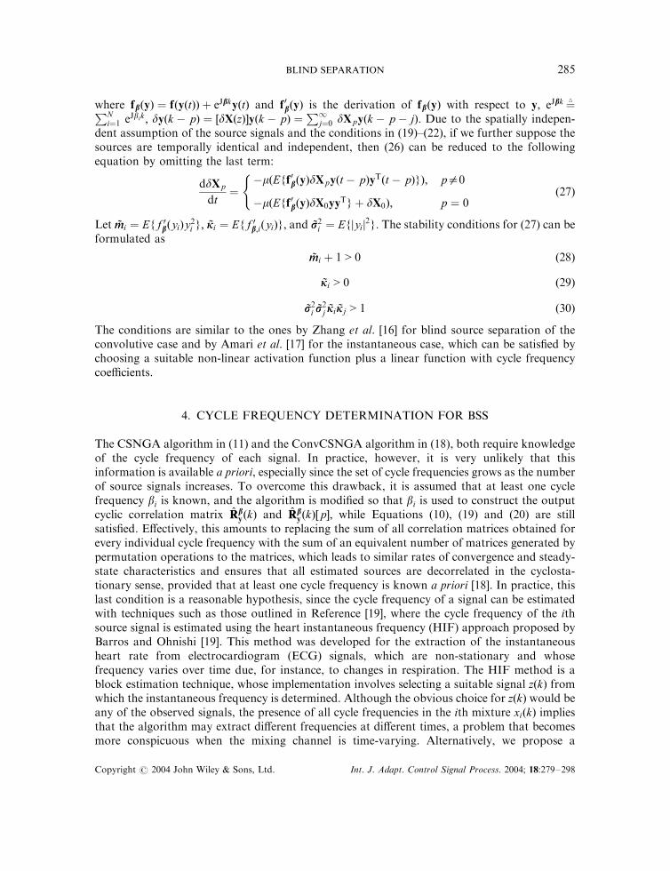
4. CYCLE FREQUENCY DETERMINATION FOR BSS

The CSNGA algorithm in (11) and the ConvCSNGA algorithm in (18), both require knowledgeof the cycle frequency of each signal. In practice, however, it is very unlikely that thisinformation is available a priori, especially since the set of cycle frequencies grows as the numberof source signals increases. To overcome this drawback, it is assumed that at least one cyclefrequency bi is known, and the algorithm is modified so that bi is used to construct the outputcyclic correlation matrix #RRb

yðkÞ and #RRbyðkÞ½p�; while Equations (10), (19) and (20) are still

satisfied. Effectively, this amounts to replacing the sum of all correlation matrices obtained forevery individual cycle frequency with the sum of an equivalent number of matrices generated bypermutation operations to the matrices, which leads to similar rates of convergence and steady-state characteristics and ensures that all estimated sources are decorrelated in the cyclosta-tionary sense, provided that at least one cycle frequency is known a priori [18]. In practice, thislast condition is a reasonable hypothesis, since the cycle frequency of a signal can be estimatedwith techniques such as those outlined in Reference [19], where the cycle frequency of the ithsource signal is estimated using the heart instantaneous frequency (HIF) approach proposed byBarros and Ohnishi [19]. This method was developed for the extraction of the instantaneousheart rate from electrocardiogram (ECG) signals, which are non-stationary and whosefrequency varies over time due, for instance, to changes in respiration. The HIF method is ablock estimation technique, whose implementation involves selecting a suitable signal zðkÞ fromwhich the instantaneous frequency is determined. Although the obvious choice for zðkÞ would beany of the observed signals, the presence of all cycle frequencies in the ith mixture xiðkÞ impliesthat the algorithm may extract different frequencies at different times, a problem that becomesmore conspicuous when the mixing channel is time-varying. Alternatively, we propose a



sequential method to estimate the cycle frequency from one of the extracted sources using theadaptive scheme in Figure 1. By modifying the HIF approach in Reference [19], a sequentialalgorithm for cycle frequency determination is concluded as follows [18]:

(i) Select one output signal and acquire a block of length B as the data becomeavailable.

(ii) Calculate the spectrogram Sðk; f Þ of zðkÞ in terms of the acquired block samples.(iii) Find the frequency value at which Sðk; f Þ attains its maximum in a given frequency

interval ½dðk�Þ � g; dðk�Þ þ g�; where dðk�Þ is the value of the driver at the previous time,and the frequency range searched is limited by g:

(iv) Divide the original signal zðkÞ into blocks, to give the signals zOðkÞ; where O is a shorttime interval.

(v) Calculate the filtered version *zzOðkÞ of zOðkÞ using a band-pass filter uðkÞ with centrefrequency dðkÞ:

(vi) Evaluate the angular instantaneous frequency for each *zzOðkÞ from oðkÞ ¼ fðk þ 1Þ �fðkÞ; fðkÞ ¼ tan�1ð�H ½ *zzOðkÞ�= *zzOðkÞÞ; where H ½ *zzOðkÞ� is the Hilbert transform of thesignal *zzOðkÞ:

(vii) Evaluate the frequency from oðkÞ; using f ðkÞ ¼ oðkÞ=2p: Then, the estimated cyclicfrequency is given by #bbHIFðkÞ ¼ 2f ðkÞ:

(viii) Use the resulting cycle frequency over this time interval to separate the sources with theConvCSNGA algorithm.

(ix) Repeat (i)–(vii) for every new block of data.

Steps (ii)–(vii) are actually specified in Figure 1 termed as ‘cycle frequency determination’.In our implementation, the windowing function hðkÞ is chosen to be the Hanning windowof length 256, the band-pass filter uðkÞ is a second-order digital filter based upon a Butterworthprototype, and the frequency range searched is limited by g ¼ 17 frequency samples. Finally,the data block size B is set to 100 samples. The method presented above implies implicitlythat the source signals have distinct cyclic frequencies and that the noise is at a low level, moredetails are found in Reference [18] for the practical problems such as identical cycle frequenciesand the robustness of the algorithm to additive noise.

)(1 kx

)(kxM

)(1 ky

)(kyN )1( BkyN )1(Ny

)1(1 Bky )1(1y

iβ ̂

-

-

+

+

Figure 1. Cycle frequency determination scheme.



5. SIMULATION STUDY

In this section, we examine the performance of the proposed algorithm by simulations both forinstantaneous mixtures and convolutive mixtures. For convolutive mixtures, we will deal withtwo kinds of data, namely, artificial convolutive mixtures and the data of real recordings.

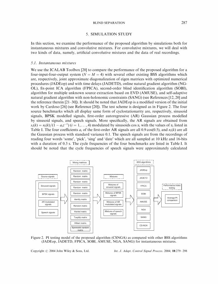
5.1. Instantaneous mixtures

We use the ICALAB Toolbox [20] to compare the performance of the proposed algorithm for afour-input-four-output system ðN ¼ M ¼ 4Þ with several other existing BSS algorithms whichare, respectively, joint approximate diagonalization of eigen matrices with optimized numericalprocedures (JADEop) and with time delays (JADETD), online natural gradient algorithm (NG-OL), fix-point ICA algorithm (FPICA), second-order blind identification algorithm (SOBI),algorithm for multiple unknown source extraction based on EVD (AMUSE), and self-adaptivenatural gradient algorithm with non-holonomic constraints (SANG) (see References [12, 20] andthe reference therein [21–30]). It should be noted that JADEop is a modified version of the initialwork by Cardoso [26] (see Reference [20]). The test scheme is designed as in Figure 2. The foursource benchmarks which all display same form of cyclostationarity are, respectively, sinusoidsignals, BPSK modelled signals, first-order autoregressive (AR) Gaussian process modelledby sinusoid signals, and speech signals. More specifically, the AR signals are obtained fromsiðkÞ ¼ niðkÞ=ð1� aiz�1Þ ði ¼ 1; . . . ; 4Þ modulated by sinusoids cos ai with the values of ai listed inTable I. The four coefficients ai of the first-order AR signals are all 0:9 cosð0:5Þ; and niðkÞ are allthe Gaussian process with standard variance 0:1: The speech signals are from the recordings ofreading four words ‘some’, ‘pick’, ‘sing’ and ‘date’ which are all sampled at 10 kHz and 16-bitswith a duration of 0:3 s: The cycle frequencies of the four benchmarks are listed in Table I. Itshould be noted that the cycle frequencies of speech signals were approximately calculated

Figure 2. PI testing model of the proposed algorithm (CSNGA) as compared with other BSS algorithms(JADEop, JADETD, FPICA, SOBI, AMUSE, NGA, SANG) for instantaneous mixtures.



according to the individual time scale and periodicity of the voiced part of each speech signal(Figure 3). The determinants and the condition values of the 11 mixing matrices are listed inTable II. The normalized performance index (PI) which is often used to evaluate theperformance of BSS algorithms is defined as

PIðkÞ ¼1

m

Xmi¼1

Xmj¼1

jpijj2

maxqjpiqj2� 1

( )þ

1

m

Xmj¼1

Xmi¼1

jpijj2

maxqjpqjj2� 1

( )ð31Þ

where pij are the entries of the global system P ¼ WH: Generally speaking, a lower valueindicates a better performance. In the test, we use the default parameters which are alreadytuned approximate optimum values for typical data, and the performance of the algorithms isevaluated by the average PIs of five trials for each algorithm which is shown in Figure 4. From

Table I. Cycle frequencies of the four benchmarks.

Benchmarks Cycle frequencies of the four source signals

Sinusoid signals ð20pÞ�1 ð10pÞ�1 3ð10pÞ�1 9ð20pÞ�1

BPSK modelled signals ð10pÞ�1 ð5pÞ�1 ð4pÞ�1 2ð5pÞ�1

AR modelled signals ð10pÞ�1 ð4pÞ�1 3ð10pÞ�1 9ð20pÞ�1

Speech signals (approximate) 180 200 150 170

0 500 1000 1500 2000 2500

-0.2

0

0. 2

s1

0 500 1000 1500 2000 2500-0.2

0

0. 2

s2

0 500 1000 1500 2000 2500-0.2

0

0. 2

s3

0 500 1000 1500 2000 2500

-0.2

0

0. 2

Samples

s4

"some"

"pick"

"sing"

"date"

Figure 3. Speech signals with cyclic properties.



Figure 4, we see that although the proposed algorithm is based on high-order statistics which isthe same as in the natural gradient algorithm and can be regarded as a new member of thenatural gradient algorithms, incorporation of the second-order cyclostationary statistics shows asuperior performance to that of NG-OL and SANG algorithms for the separation of the firstthree source signals (see Figure 4 (a)–(c)). The proposed algorithm has a similar performance forthe separation of the sine wave sources as the second-order methods such as AMUSE and SOBI,however, the high-order statistics ICA algorithm (such as JADEop and NG-OL) fail toreconstruct such sources because they are dependent (see Figure 4(a)). It should be noted that

Table II. Determinants and condition values of the mixing matrices.

Mixing matrices H1 H2 H3 H4 H5 H6

Determinants �0.46 0.26 0.55 �1.74 0.24 1Condition values 10.74 9.94 4.93 2.28 5.63 1

Mixing matrices H7 H8 H9 H10 H11

Determinants 0.75 1.0e�3 0.41 1.33e�7 3.33e�4Condition values 5.04 94.75 5.32 1.98e+4 10.08

Figure 4. PI comparison of the proposed algorithm (CSNGA) with several other BSS algorithms(JADETD, NG-OL, FPICA, SOBI, AMUSE, SANG, JADEop) for the separation of four kinds of signalswith cyclostationary properties. The four signals are, respectively, sinusoid signals, BPSK modelled signals,

AR modelled signals and speech signals.



other high-order statistics based methods such as JADETD and FPICA, similarly, do notperform well for such sources either. However, there exists slight difference (even inconsistentresults) in performance measurement due to the various learning mechanism in these methods(see Reference [20] for more details). From Figure 4(d), it can be seen that considering the cyclicproperties of the sources also generates a better performance as compared to the NG-OL for theseparation of typical speech signals with cycle-like properties, however, the performance is notas good as that of the SANG algorithm. This is not unexpected since the speech signals are non-stationary and their average magnitudes change rapidly and the SANG algorithm introducesnon-holonomic constraints in the NG learning process so that it can adapt to rapid changes inthe magnitudes of the source signals. In our simulations, the proposed algorithm without suchconstraints can however generate a similar separation performance as the SANG algorithm.

5.2. Convolutive mixtures

5.2.1. Artificially convolutive mixtures. In the case of artificially convolved mixtures, a two-input-two-output (TITO) system ðN ¼ M ¼ 2Þ is considered for simplicity. The resemblancebetween the original and the reconstructed source waveforms is measured by their mean squareddifference

e2ðdBÞ ¼ 10 log ð1=N ÞXNi¼1

E½jyiðkÞ � siðkÞj2�

( )ð32Þ

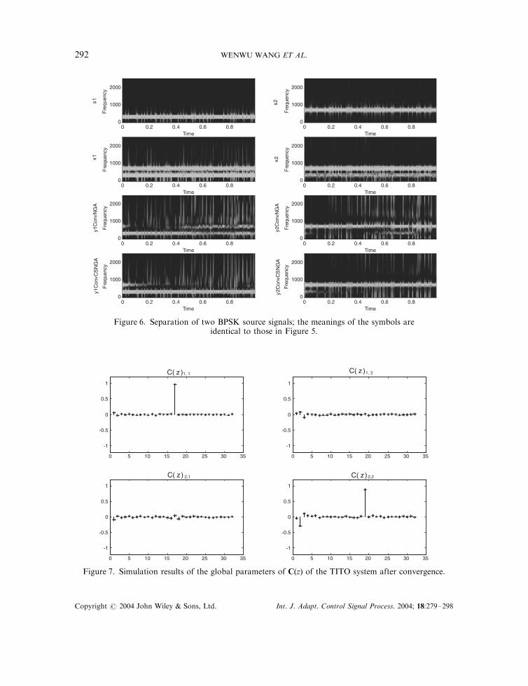
(assuming the signals are zero-mean and unit-variance). First, we use sinusoid signals to test theperformance of the proposed algorithm, where the sinusoid signal can be treated as a degeneratecase of cyclostationary signals, we appreciate that such a signal will only excite one ofthe frequency components of a general convolutive system. The two source signals areset, respectively, to be s1ðiÞ ¼ sin ð0:4iÞ; s2ðiÞ ¼ sin ð0:9iÞ: The two sources are convolved byFIR filters with entries Hð1; :; 1Þ ¼ ½1 1 � 0:75 0:9�; Hð2; :; 1Þ ¼ ½0:5 � 0:3 0:2 0:2�; Hð1; :; 2Þ ¼½�0:2 0:4 0:7 0:2�; Hð2; :; 2Þ ¼ ½0:2 1 0 0:9�: The other parameters are m ¼ 0:004; and r ¼ 0:1:The two cyclic frequencies are, respectively ð5pÞ�1 and 9ð20pÞ�1: It should be noted that, ingeneral, changing filter length L would change the performance of the separation quality [5]. Ithas been shown that if we increase L; we may obtain an improved separation performance ascompared with a shorter length, however, the performance will also suffer from the length of thedata samples being used when increasing L; and it may degraded seriously when the data lengthis limited. Additionally, for the time-domain implementation, increasing L indicates a significantincrease of the filter coefficients to be estimated. This will lead to a problem of much morecomputational complexity as compared to that of the frequency domain implementation. In thefollowing simulations, we use L ¼ 32 if it is not specified. The separation results are shown inFigure 5, and the performance indices are, respectively, �8:36 and �4:35 dB: In the secondsimulation (see Figure 6), two BPSK signals modulated by sinusoids of carrier frequenciesð5pÞ�1 and 9ð20pÞ�1; which can be treated as the other general sets of signals with cyclicproperty, are chosen as the source signals. The mixing matrix and the parameters are identical tothose in the first simulation. The performance indices are, respectively, �14:95 and �4:45 dB: Inboth simulations, the cyclic frequencies are chosen to be the same as the carrier frequencies andthe step size is unchanged for two simulations (allowed for comparison). Both simulation resultsindicate that the proposed algorithm has improved performance over the natural gradient



algorithm in recovering the cyclic property and waveform of the cyclostationary signals fromthe convolutive mixtures. In the third simulation (setting the same parameters as in the secondsimulation), the separability of the proposed algorithm is shown in Figure 7, where theconvolutive mixtures are successfully separated from the two channels in terms of thedistribution of the global parameters. By resorting to the multichannel row intersymbolinterference (Row ISI) defined as

ISIðiÞ ¼

Pi

Pk jcijðkÞj2 �maxj;k jcij ðkÞj

2

maxj;k jcijðkÞj2

ð33Þ

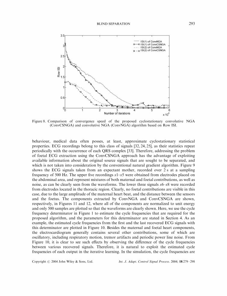
where cij are the filter elements of the global system Cðz; kÞ; we can further measure theconvergence speed of the proposed algorithm. From Figure 8, we see that the proposedalgorithm needs a considerably smaller number of iterations to converge to the steady-statevalue, e.g. for ISI(1) to reach 0.01, there is approximately 30% reduction in convergence time,thereby further indicating an improved convergence performance [15].

5.2.2. Real recordings. Biomedical data frequently originate from periodic phenomena, such asbreathing, tremor or contraction of the cardiac muscle [31], and since cyclostationary signals,man-made or otherwise, arise when the underlying process generating them has oscillatory

Time

Fre

quen

cy

0 0.05 0.1 0.15 0.2 0.25 0.3 0.350

1000

2000

Time

Fre

quen

cy

0 0.05 0.1 0.15 0.2 0.25 0.3 0.350

1000

2000

Time

Fre

quen

cy

0 0.05 0.1 0.15 0.2 0.25 0.3 0.350

1000

2000

Time

Fre

quen

cy

0 0.05 0.1 0.15 0.2 0.25 0.3 0.350

1000

2000

Time

Fre

quen

cy

0 0.05 0.1 0.15 0.2 0.25 0.3 0.350

1000

2000

Time

Fre

quen

cy

0 0.05 0.1 0.15 0.2 0.25 0.3 0.350

1000

2000

Time

Fre

quen

cy

0 0.05 0.1 0.15 0.2 0.25 0.3 0.350

1000

2000

Time

Fre

quen

cy

0 0.05 0.1 0.15 0.2 0.25 0.3 0.350

1000

2000

s1 s2

x1 x2

y1C

onvN

GA

y2C

onvN

GA

y2C

onvC

SN

GA

y1C

onvC

SN

GA

Figure 5. Separation of convolutive mixtures of two sinusoid signals: s1 and s2 are two sources,x1 and x2 are the two convolutive mixtures, y1ConvNGA and y2ConvNGA are the recoveredsignals by the natural gradient algorithm, y1ConvCSNGA and y2ConvCSNGA are the recovered

signals by the proposed method.



Time

Fre

quen

cy

0 0.2 0.4 0.6 0.80

1000

2000

Time

Fre

quen

cy

0 0.2 0.4 0.6 0.80

1000

2000

Time

Fre

quen

cy

0 0.2 0.4 0.6 0.80

1000

2000

Time

Fre

quen

cy

0 0.2 0.4 0.6 0.80

1000

2000

Time

Fre

quen

cy

0 0.2 0.4 0.6 0.80

1000

2000

Time

Fre

quen

cy

0 0.2 0.4 0.6 0.80

1000

2000

Time

Fre

quen

cy

0 0.2 0.4 0.6 0.80

1000

2000

Time

Fre

quen

cy

0 0.2 0.4 0.6 0.80

1000

2000

s1 s2

x1 x2

y1C

onvN

GA

y2C

onvN

GA

y1C

onvC

SN

GA

y2C

onvC

SN

GA

Figure 6. Separation of two BPSK source signals; the meanings of the symbols areidentical to those in Figure 5.

0 5 10 15 20 25 30 35

-1

-0.5

0

0.5

1

C( z )

0 5 10 15 20 25 30 35

-1

-0.5

0

0.5

1

C( z )

0 5 10 15 20 25 30 35

-1

-0.5

0

0.5

1

C( z)

0 5 10 15 20 25 30 35

-1

-0.5

0

0.5

1

C( z)

1, 1 1, 2

2,2 2,1

Figure 7. Simulation results of the global parameters of CðzÞ of the TITO system after convergence.



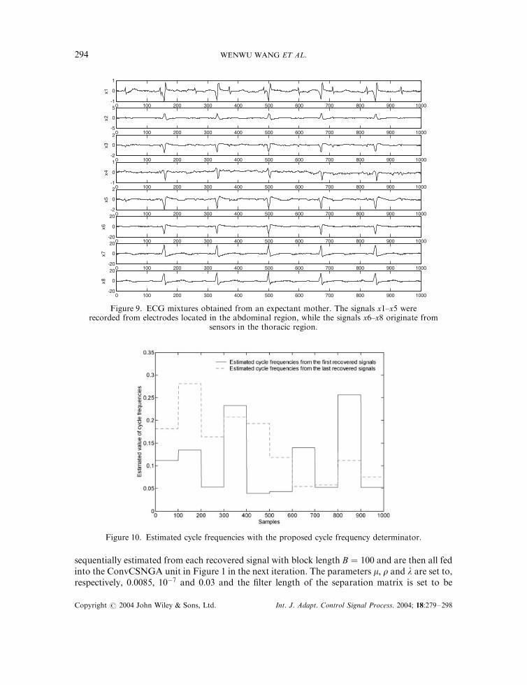
behaviour, medical data often posses, at least, approximate cyclostationary statisticalproperties. ECG recordings belong to this class of signals [32, 24, 25], as their statistics repeatperiodically with the occurrence of each QRS complex [33]. Therefore, addressing the problemof foetal ECG extraction using the ConvCSNGA approach has the advantage of exploitingavailable information about the original source signals that are sought to be separated, andwhich is not taken into consideration by the conventional natural gradient algorithm. Figure 9shows the ECG signals taken from an expectant mother, recorded over 2 s at a samplingfrequency of 500 Hz: The upper five recordings x1–x5 were obtained from electrodes placed onthe abdominal area, and represent mixtures of both maternal and foetal contributions, as well asnoise, as can be clearly seen from the waveforms. The lower three signals x6–x8 were recordedfrom electrodes located in the thoracic region. Clearly, no foetal contributions are visible in thiscase, due to the large amplitude of the maternal heart beat, and the distance between the sensorsand the foetus. The components extracted by ConvNGA and ConvCSNGA are shown,respectively, in Figures 11 and 12, where all of the components are normalized to unit energyand only 500 samples are plotted so that the waveforms are clearly shown. Here, we use the cyclefrequency determinator in Figure 1 to estimate the cycle frequencies that are required for theproposed algorithm, and the parameters for this determinator are stated in Section 4. As anexample, the estimated cycle frequencies from the first and the last recovered ECG signals withthis determinator are plotted in Figure 10. Besides the maternal and foetal heart components,the electrocardiogram generally contains several other contributions, some of which areoscillatory, including respiratory motion, tremor artifacts and periodic power line noise. FromFigure 10, it is clear to see such effects by observing the difference of the cycle frequenciesbetween various recovered signals. Therefore, it is natural to exploit the estimated cyclefrequencies of each output in the iterative learning. In the simulation, the cycle frequencies are

Figure 8. Comparison of convergence speed of the proposed cyclostationary convolutive NGA(ConvCSNGA) and convolutive NGA (ConvNGA) algorithm based on Row ISI.



sequentially estimated from each recovered signal with block length B ¼ 100 and are then all fedinto the ConvCSNGA unit in Figure 1 in the next iteration. The parameters m; r and l are set to,respectively, 0:0085; 10�7 and 0:03 and the filter length of the separation matrix is set to be

Figure 10. Estimated cycle frequencies with the proposed cycle frequency determinator.

0 100 200 300 400 500 600 700 800 900 1000-1

0

1

x1

0 100 200 300 400 500 600 700 800 900 1000-5

0

5x2

0 100 200 300 400 500 600 700 800 900 1000-2

0

2

x3

0 100 200 300 400 500 600 700 800 900 1000-1

0

1

x4

0 100 200 300 400 500 600 700 800 900 1000-2

0

2

x5

0 100 200 300 400 500 600 700 800 900 1000-20

0

20

x6

0 100 200 300 400 500 600 700 800 900 1000-20

0

20

x7

0 100 200 300 400 500 600 700 800 900 1000-20

0

20

x8

Figure 9. ECG mixtures obtained from an expectant mother. The signals x1–x5 wererecorded from electrodes located in the abdominal region, while the signals x6–x8 originate from

sensors in the thoracic region.



L ¼ 32: Since the source signals are real valued, the proposed algorithm for real value is used inthis case. Observing the recovered signals in Figure 12, we see that four maternal componentsand two foetal heart components are successfully extracted from the mixtures, and theremaining two signals may be the other interferences and noise components, which is similar to

0 50 100 150 200 250 300 350 400 450 500-1

0

1ConvNGA

0 50 100 150 200 250 300 350 400 450 500-1

0

1

y2

0 50 100 150 200 250 300 350 400 450 500-1

0

1

y3

0 50 100 150 200 250 300 350 400 450 500-1

0

1

y4

0 50 100 150 200 250 300 350 400 450 500-1

0

1

y5

0 50 100 150 200 250 300 350 400 450 500-1

0

1

y6

0 50 100 150 200 250 300 350 400 450 500-1

0

1

y7

0 50 100 150 200 250 300 350 400 450 500-1

0

1

Samples

y8y1

Figure 11. Separation results with ConvNGA algorithm for ECG signals in Figure 9.

0 50 100 150 200 250 300 350 400 450 500-1

0

1

y8

0 50 100 150 200 250 300 350 400 450 500-1

0

1

y7

0 50 100 150 200 250 300 350 400 450 500-1

0

1

y6

0 50 100 150 200 250 300 350 400 450 500-1

0

1

y5

0 50 100 150 200 250 300 350 400 450 500-1

0

1

y4

0 50 100 150 200 250 300 350 400 450 500-1

0

1

y3

0 50 100 150 200 250 300 350 400 450 500-1

0

1

y2

0 50 100 150 200 250 300 350 400 450 500-1

0

1

y1

ConvCSNGA

Figure 12. Separation results with ConvCSNGA algorithm for the ECG signals in Figure 9.



that with ConvNGA algorithm (see Figure 11). Comparing y1 and y2 in Figure 12 with thecorresponding components y3 and y8 in Figure 11, it can be seen that the foetal contributions ofthe ECG signals recovered by the ConvCSNGA algorithm have improved waveforms which arestronger and smoother with ConvCSNGA than those with the ConvNGA algorithm. Asdiscussed in Reference [18], the robustness of the proposed algorithm for real recordings highlyrelies on the estimated cycle frequencies, and using a set of cycle frequencies from one outputusually reveals a different performance from the other output. Exploiting the whole cyclefrequencies from all outputs reveals a better performance as compared with exploiting only oneoutput.

6. CONCLUSIONS

A blind source separation algorithm for separating convolutive mixtures of cyclostationarysignals has been presented. Exploiting the statistical cyclostationarity of signals with the naturalgradient algorithm for convolutive mixtures leads to a new member (ConvCSNGA) of thefamily of natural gradient algorithms in adaptive source separation. One of the importantimplementation problems, i.e. cycle frequency determination for each estimated source signals isdetailed and an efficient sequential algorithm for cycle frequency estimation based on HIF isproposed. Simulation results have shown that exploiting the cyclostationarity of signals in theblind source separation algorithm leads to faster speed of convergence, together with a betterperformance for the separation of the convolved cyclostationary signals, in particular in formsof shape preservation, as compared to Amari’s conventional natural gradient algorithm forconvolutive mixtures.

APPENDIX A

Derivation of Equation (11) (see Reference [18]): In terms of yðkÞ ¼ WðkÞxðkÞ; the output cycliccorrelation matrix is given by

*RRbyðkÞ ¼

XNi¼1

heJbikyðkÞyTðkÞi ¼XNi¼1

WðkÞRbix ðkÞW

TðkÞ

¼WðkÞXNi¼1

Rbix ðkÞ

!WTðkÞ ¼ WðkÞð *RRb

xðkÞÞWTðkÞ ðA1Þ

where *RRbxðkÞ ¼

PNi¼1 Rbi

x ðkÞ: Applying the stochastic gradient descent, the gradient of (8) is

@rðWðkÞÞ@WðkÞ

¼ fðyðkÞÞxTðkÞ � ðW�1ðkÞÞT þWðkÞ *RRbxðkÞ � ðW�1ðkÞÞT ðA2Þ

and the update equation of (11) can be easily obtained by post-multiplying WHðkÞWðkÞ to thetwo sides of Equation (A2).



Derivation of Equations (14) and (15):

dflog detð *RRbyðkÞÞg ¼ d log det

XNi¼1

heJbikyðkÞyTðkÞi

" #( )

’ d log detXNi¼1

eJbik

!hyðkÞyTðkÞi

" #( )

¼ d N logXNi¼1

eJbik

!( )þ dflog dethyðkÞyTðkÞig

¼ d N logXNi¼1

eJbik

!( )þ dflog det *RRxg

þ 2 TrfdWðz; kÞW�1ðz; kÞg ðA3Þ

dfTrð *RRbyðkÞÞg ¼d Tr

XNi¼1

eJbik

!hyðkÞyTðkÞi

!( )

’XNi¼1

eJbik

!dXNi¼1

hy2i ðkÞi

( )

¼ 2XNi¼1

eJbik

!XNi¼1

hyiðkÞ dyiðkÞi

¼ 2XNi¼1

eJbik

!hyTðkÞ dyðkÞi

¼ 2XNi¼1

eJbik

!hyTðkÞ dXðz; kÞyðkÞi ðA4Þ

ACKNOWLEDGEMENT

This work was supported by the Engineering and Physical Sciences Research Council (EPSRC) of the U.K.

REFERENCES

1. Haykin S. Unsupervised Adaptive Filtering. Wiley: New York, 2000.2. Wang W, Chambers JA, Sanei S. A joint diagonalization method for convolutive blind separation of nonstationary

sources in the frequency domain. In Proceedings of the ICA2003, 939–944, Nara, Japan, April 1–4, 2003.3. Amari S, Douglas S, Cichocki A, Yang H. Novel on-line algorithms for blind deconvolution using natural gradient

approach. Proceedings of the SYSID-97, Kitakyushu, Japan, July, 1997; 1057–1062.4. Smaragdis P. Blind separation of convolved mixtures in the frequency domain. Neurocomputing 1998; 22:21–34.5. Parra L, Spence C. Convolutive blind source separation of nonstationary sources. IEEE Transactions on Speech and

Audio Processing 2000; 8(5):320–327.6. Mansour A, Jutten C, Loubaton P. Adaptive subspace algorithm for blind separation of independent sources in

convolutive mixtures. IEEE Transactions on Signal Processing 2000; 48(2):583–586.



7. Meraim KA, Xiang Y, Manton JH, Hua Y. Blind source separation using second-order cyclostationary statistics.IEEE Transactions on Signal Processing 2001; 49(4):694–701.

8. Ferreol A, Chevalier P. On the behavior of current second and higher order blind source separation methods forcyclostationary sources. IEEE Transactions on Signal Processing 2000; 48(6):1712–1725.

9. Jafari MG, Chambers JA, Mandic DP. Natural gradient algorithm for cyclostationary sources. IEE ElectronicLetters 2002; 38(7):758–759.

10. Gardner WA. Statistical Spectral Analysis: A Nonprobabilistic Theory. Prentice-Hall: Englewood Cliffs, NJ; 1988.11. Jafari MG, Alty S, Chambers JA. A new natural gradient algorithm for cyclostationary sources. IEE

Proceedings}Vision Image and Signal Processing 2004; 151(1).12. Cichocki A, Amari S. Adaptive Blind Signal and Image Processing: Learning Algorithms and Applications. Wiley:

New York, 2002.13. Cardoso JF, Laheld B. Equivariant adaptive source separation. IEEE Transactions on Signal Processing 1996;

44(12):3017–3030.14. Choi S, Cichocki A, Amari S. Equivariant nonstationary source separation. Neural Networks 2002; 15(1):121–130.15. Wang W, Jafari MG, Sanei S, Chambers JA. Blind separation of convolutive mixtures of cyclostationary sources

using an extended natural gradient method. In Proceedings of the ISSPA2003, II: 93–96, Paris, France, July 1–4,2003.

16. Zhang L, Cichocki A, Amari S. Geometrical structures of FIR manifold and their application to multichannel blinddeconvolution. Journal of VLSI for Signal Processing 2002; 31 31–44.

17. Amari S, Chen TP, Cichocki A. Stability analysis of learning algorithms for blind source separation. NeuralNetworks 1997; 10(8):1345–1351.

18. Jafari MG. Novel sequential algorithms for blind source separation of instantaneous mixtures. Ph.D. Thesis ofKing’s College, University of London, 2002.

19. Barros AK, Ohnishi N. Heart instantaneous frequency (HIF): an alternative approach to extract heart ratevariability. IEEE Transactions on Biomedical Engineering 2001; 48(7):850–855.

20. Cichocki A, Amari S, Siwek K, et al. ICALAB Toolboxes. http://www.bsp.brain.riken.go.jp.21. Tong L, Soon V, Huang YF, Liu R. Indeterminacy and identifiability of blind identification. IEEE Transactions on

CAS of VLSI for Signal Processing 1991; 38:499–509.22. Tong L, Inouye Y, Liu R. Waveform-preserving blind estimation of multiple independent sources. IEEE

Transactions on Signal Processing 1993; 41(7):2461–2470.23. Belouchrani A, Abed-Meraim K, Cardoso JF, Moulines E. A blind source separation technique using second order

statistics. IEEE Transactions on Signal Processing 1997; 45(2):434–444.24. De Lathauwer L, De Moor B, Vandewalle J. Fetal electrocardiogram extraction by blind source subspace

separation. IEEE Transactions on Biomedical Engineering}Special Topic Section on Advances in Statistical SignalProcessing for Medicine 2000; 47(5):567–572.

25. Zarzoso V, Nandi AK. Noninvasive fetal electrocardiogram extraction: blind separation versus adaptive noisecancellation. IEEE Transactions on Biomedical Engineering 2001; 48(1):12–18.

26. Cardoso JF, Souloumiac A. Jacobi angles for simultaneous diagonalization. SIAM Journal of Matrix Analysis andApplications 1996; 17(1) 161–164.

27. Georgiev P, Cichocki A. Robust blind source separation utilizing second and fourth order statistics. In InternationalConference on Artificial Neural Networks (ICANN2002) 2002; Mardrid, Spain, August, 2002.

28. Hyvarinen A, Oja E. A fast fixed-point algorithm for independent component analysis. Neural Computation 1997;9(7):1483–1492.

29. Amari S, Cichocki A, Yang HH. A new learning algorithm for blind signal separation. Advances in NeuralInformation Processing Systems, NIPS-1995, vol. 8 MIT Press: Cambridge, MA, 1996; 757–763.

30. Amari S, Cichocki A. Adaptive blind signal processing}neural network approaches. Proceedings IEEE 1998;86:1186–1187.

31. Timmer J. Power of surrogate data testing with respect to nonstationarity. Physical Review E 1998; 58:5153–5156.32. Saha S, Ramakrishnan AG. Transmission of chosen transform coefficients of normalized cardiac beats for

compression. Proceedings of the ICASSP, 1997; vol. 3, 1901–1904.33. Speirs CA, Soraghan JJ, Stewart RW, Byrne S. Least squares time sequenced adaptive filtering for the detection of

fragmented micropotentials. http://www.spd.eee.strath.ac.uk/research.html, 1995.



Blind separation of convolutive mixtures of cyclostationary signals

Documents

Transcript of Blind separation of convolutive mixtures of cyclostationary signals