Ocular Reduction in EEG Signals Based on Adaptive Filtering, Regression

and Blind Source Separation

S. ROMERO,1,2 M. A. MANANAS,1,2 and M. J. BARBANOJ3

1Department of Automatic Control (ESAII), Biomedical Engineering Research Center, Universitat Politecnica de Catalunya(UPC), Barcelona, Spain; 2CIBER de Bioingenierıa, Biomateriales y Nanomedicina (CIBER-BBN), Barcelona, Spain; and 3DrugResearch Center (CIM), Research Institute of Sant Pau Hospital, Department of Pharmacology and Therapeutics, Universitat

Autonoma de Barcelona (UAB), Barcelona, Spain

(Received 11 April 2008; accepted 20 October 2008; published online 5 November 2008)

Abstract—Quantitative electroencephalographic (EEG) anal-ysis is very useful for diagnosing dysfunctional neural statesand for evaluating drug effects on the brain, among others.However, the bidirectional contamination between electro-oculographic (EOG) and cerebral activities can mislead andinduce wrong conclusions from EEG recordings. Differentmethods for ocular reduction have been developed but onlyfew studies have shown an objective evaluation of theirperformance. For this purpose, the following approacheswere evaluated with simulated data: regression analysis,adaptive filtering, and blind source separation (BSS). In thefirst two, filtered versions were also taken into account byfiltering EOG references in order to reduce the cancellationof cerebral high frequency components in EEG data.Performance of these methods was quantitatively evaluatedby level of similarity, agreement and errors in spectralvariables both between sources and corrected EEG record-ings. Topographic distributions showed that errors werelocated at anterior sites and especially in frontopolar andlateral–frontal regions. In addition, these errors were higherin theta and especially delta band. In general, filtered versionsof time-domain regression and of adaptive filtering with RLSalgorithm provided a very effective ocular reduction. How-ever, BSS based on second order statistics showed the highestsimilarity indexes and the lowest errors in spectral variables.

Keywords—Electroencephalography (EEG), Electrooculog-

raphy (EOG), Ocular artifacts, Regression analysis, Adaptive

filtering, Blind source separation (BSS), Independent com-

ponent analysis (ICA).

INTRODUCTION

Quantitative analysis of electroencephalographic(EEG) signals is a helpful support in the diagnosis ofpsychiatric and neurological disorders, and in theevaluation of drug effects in functional states of the

brain. EEG changes are often quantified by the cal-culation of spectral variables in different frequencybands of clinical interest: delta, theta, alpha, and beta.It is known that non-cortical interferences, such asheart, ocular, and muscular activities, contribute toEEG recordings. Procedures to detect and removethese artifacts are very important and necessary be-cause they could lead to wrong results and conclusions.

Ocular artifacts are the most relevant interferencebecause they occur very frequently and their amplitudecan be several times larger than brain scalp potentials.As the eyeball moves, the electric field composed bycornea and retina changes and it produces the elec-trooculographic (EOG) signals. Additionally, someneural activity is recorded by EOG electrodes becausethey are located near the head. Muscle activity asso-ciated with the eyes or near them can also interfere inthe EOG signal. Ocular activity propagates across thescalp: vertical ocular projection following the anterior–posterior direction, and horizontal mainly affectinglateral–frontal scalp regions.7

Linear regression analysis is the most common ap-proach for reducing eye movement artifacts. Thismethod estimates and removes the EOG componentexisting in each EEG lead. However, regression pro-cedures do not take into account the bidirectionalcontamination, i.e., EOG recording is also contami-nated by cerebral activity, and consequently this cere-bral information could be relevant and can also becancelled in the EEG recordings after linear subtrac-tion. Gasser et al.11 proposed previously to applyregression procedure a low pass filtering of EOG sig-nals in order to reduce the cancellation of high fre-quency cerebral components from EEG data.

He et al.12 proposed the adaptive filtering byrecursive least squares (RLS) algorithm which wasapplied to simulated data in He et al.13 in order tocompare with time-regression procedure. However, the

Address correspondence to S. Romero, Department ofAutomatic

Control (ESAII), Biomedical Engineering Research Center, Univer-

sitat Politecnica de Catalunya (UPC), Barcelona, Spain. Electronic

mail: sergio.romero-lafuente@upc.edu

Annals of Biomedical Engineering, Vol. 37, No. 1, January 2009 (� 2008) pp. 176–191

DOI: 10.1007/s10439-008-9589-6

0090-6964/09/0100-0176/0 � 2008 Biomedical Engineering Society

176

authors did not consider in their study the bidirectionalcontamination. They recognized that it would deteri-orate the method and they pointed out modificationssuch as smoothing the reference EOG.

In addition, other approaches based on BlindSource Separation (BSS) have been proposed.18,22,31

BSS procedures decompose the multichannel EOG andEEG recordings into source components. Sources,which are related with artifacts, are deleted byremoving their contributions onto the scalp sensors.The first proposed component-based procedure wasPrincipal Component Analysis (PCA).20 However, ithas several drawbacks related to the assumption oforthogonality between neural and ocular activities, andthe difficulty to separate eye movement artifacts fromcerebral activity when their amplitudes are similar.More recent approaches use blind source extractionbased on Independent Component Analysis (ICA).Assumption for ICA-based techniques is that sourcesmust be statistically independent, not just uncorre-lated, and this is mostly true with regard to brain andocular components.

There are different algorithms and principles toestimate the components, generally based on secondorder and higher order statistics. However, most of theEEG studies with ICA application identify the arti-factual source components by visual inspection fol-lowing a time-consuming subjective criterion.Moreover, quantitative evaluation of the performanceof each ocular correction method is difficult because itwould be necessary to get available previous knowl-edge corresponding to the true ocular and cerebralactivities, and this is not possible because they cannotbe separately measured due to bidirectional contami-nation. There have been few empirical studies mea-suring the effectiveness of ocular reduction techniqueson simulated data composed by mixtures of cerebraland ocular activities.19,32 However, these studiesshowed opposite conclusions: regression and PCAbased algorithms were suggested in Wallstrom et al.,32

adaptive filtering was proposed in He et al.,12 and BSStechniques based on second-order statistics were rec-ommended in Kierkels et al.19 and Romero et al.25 inspite of adaptive filtering was not evaluated in both.Moreover, in spite of the theoretical advantages of BSSbased approaches, a very recent study based on realdata and using expert scorers for identifying ocularartifacts concluded that regression procedure couldsignificantly reduce ocular artifacts better than ICAwhen few EEG channels were available.27

Regarding simulated data, in Wallstrom et al.32

coefficients for the linear mixture were determinedbased partially on normalizing random variates. Dueto this random mixture, simulated EEG signals did notcorrespond to specific EEG leads. In Kierkels et al.19

forced and fast ocular movements were simulated byBoundary element method (BEM). BEM calculatedthe potential at different positions in an arbitraryshape volume, and with representative tissues con-ductivity values taken from literature. Furthermore,the location of simulated brain dipoles was chosenrandomly based on real data from one EEG channel.This study was based on situations with open eyes. InHe et al.13 an arbitrary gain function for ocularpropagation was used to obtain simulated EEG andEOG signals. This function was frequency dependentand constructed based on Gasser et al.10 In Romeroet al.,25 simulated data was generated from spontane-ous EOG and EEG signals with closed eyes and withnormal (not fast forced) eye movements, which is thecommon procedure used in clinical routine. The sim-plest linear instantaneous mixtures were carried out byfactors from regression coefficients and by using EEGrecordings considered free of ocular artifacts with a notvery restrictive condition. In the present study, simu-lated EEG and EOG data were obtained by moregeneral linear mixtures whose coefficients were calcu-lated by means of multi-input single-output (MISO)linear models applied to a database composed of realEEG and EOG recordings. A more restrictive condi-tion than used in Romero et al.25 was applied in orderto consider EEG recordings more free of artifacts.Bidirectional contamination, where EOG recordingsare also interfered by some cerebral activity, was alsotaken into account by linear mixtures in both direc-tions.

In this study, a fully automatic procedure for ocularcorrection from spontaneous EEG signals based onBSS described in Romero et al.25 was used. Theobjective of the present study was twofold. The firstaim was to generate simulated EEG and EOG signalsin order to reproduce a real clinical situation in prac-tice. It was achieved by obtaining a proper propaga-tion model of cerebral and ocular activities across thescalp based on the theory of system identification. Thesecond aim was to evaluate the performance of dif-ferent ocular reduction methods (linear regression,adaptive filtering and BSS) on this simulated data. Thisevaluation was quantitatively carried out by level ofsimilarity, agreement, and spectral target variablesused commonly in clinical EEG studies.

METHODOLOGY

Subjects and Instrumentation

Twenty-four young healthy volunteers of eithergender (aged 22.50 ± 3.75 years) were selected for thestudy from a larger database. Spontaneous EEG and

Ocular Reduction in EEG Signals 177

EOG signals, sampled at 100 Hz, were acquired during10 non-consecutive 3-min periods following a vigi-lance-controlled condition with eyes closed. During thevigilance-controlled recordings, the experimenter triedto keep the volunteers alert by acoustic stimulation.Twelve subjects with normal-high eye movements(called ‘ocular group’) were selected following visualinspection of EOG signals. The remaining 12 volun-teers (called ‘cerebral group’) were carefully chosenbased on the criterion of no apparent eye movements(3 consecutive minutes with EOG amplitudes lowerthan 25 lV). Nineteen EEG recordings were obtainedby means of scalp electrodes placed according to theinternational 10/20 system: Fp1, Fp2, F7, F3, Fz, F4,F8, T3, C3, Cz, C4, T4, T5, P3, Pz, P4, T6, O1, andO2, referenced to averaged mastoids. Additionally,vertical and horizontal EOG (VEOG and HEOG,respectively) signals were recorded. The VEOG signalwas acquired from mid-forehead (2.5 cm above thepupil) to the average of one electrode below the left eyeand one electrode below the right eye (2.5 cm belowthe pupil). The HEOG signal was obtained from theouter canthi. Multichannel EOG and EEG signalswere recorded using a band pass filter between 0.3 and45 Hz.

Simulated Data

Simulated EEG Signals

Neural sources (EEGs) corresponding to 3-minconsecutive epochs were obtained from the 19 EEGchannels for each subject belonging to ‘cerebral group’and selected from the entire large database. Theselection criterion was that no samples from VEOGand HEOG signals exceeded 25 lV. This threshold waslower than 40 lV, which was used in a previousstudy,25 in order to better consider a reduced potentialocular activity in EEG data. Neural sources were ob-tained by high-pass filtering the EEG channels with acut-off frequency of 0.5 Hz in order to reduce very lowfrequency components which could be possibly morerelated to ocular activity. Interference from ocularactivity was added to the neural sources. This inter-ference was calculated by estimation of linear modelsbetween EOG and EEG recordings following theprocedure explained below.

Ten 5-s epochs with high EOG activity were chosenfrom each one of the 12 volunteers belonging to the‘ocular group.’ A multi-input single-output (MISO)linear model was estimated for each 5-s epoch and foreach lead. Models had two inputs corresponding toVEOGO and HEOGO signals (subindexO referred tosignals derived from the ‘ocular group’), and oneoutput that was each one of the 19 EEGO channels.

Due to bidirectional contamination, it is well knownthat cerebral activity also affects to EOG signals. Thisactivity was reduced for a better estimation of modelsin order to obtain the interferences from ocular activ-ity. For this purpose, in each model, EEGO and EOGO

channels, corresponding to outputs and inputs,respectively, were low-pass filtered with the cut-offfrequency corresponding to highest value of the 99%(f99) of the total energy of these VEOGO and HEOGO

signals. Thus, the remainder 1% of signal energy wasnot considered as ocular activity (neural activity,electrode noise, power line interference, etc.) in theEOGO recordings. The 99% cut-off frequencies ob-tained were 6.34 ± 4.04 and 8.20 ± 5.01 Hz forVEOGO and HEOGO, respectively, as mean andstandard deviation for all epochs and volunteers. Thisconsideration was supported by some studies whichsuggested that most of the high frequency range in theEOG signal is of neural origin.11 Besides, this low-passfiltering procedure on EOGO and EEGO did not causeapparently shift delays or variations in the ocularwaveform.

A linear autoregressive with exogenous inputARX(N, M) structure, that is described in Eq. (1), wasused for the parametric model in each i lead (i = Fp1,Fp2, …, O1, and O2), and p epoch (p = 1, 2, …, 10).

EEGOi pðnÞ þXN�1

k¼1ai pðkÞ � EEGOi pðn� kÞ

¼XM�1

k¼0b1i pðkÞ � VEOGO pðn� kÞ

þXM�1

k¼0b2i pðkÞ �HEOGO pðn� kÞ þ e ðnÞ ð1Þ

where n represents the sample time; aip, b1ip, and b2ipdenote the unknown model parameters; N and M arethe orders associated with the output and the inputs,respectively; and e(n) is the unknown error mapping.21

The same order M for both inputs was consideredbecause they corresponded to the same kind of activity,ocular, whose propagation is wanted to be modeled;and this propagation takes place in the same medium,through the head, and the same directions: from EOGchannels to EEG leads. Akaike’s final prediction error(FPE) was used to select the ARX model orders. Fig-ure 1 shows the FPE as a function of different ordersfor output and inputs. The orders selected for outputand inputs were 4 and 3, respectively, that corre-sponded to a FPE low enough and it did not decreasesensitively with higher orders. Estimation of modelparameters was implemented by least squares estima-tion method, using QR-factorization for overdeter-mined linear equations.

ROMERO et al.178

Once the parameters for each of the 10 ARXmodels were estimated for each EEG lead in eachvolunteer, two frequency responses (for both verticaland horizontal ocular activity) for every model wereevaluated. These 10 frequency responses were aver-aged in spectral domain for both VEOGO and HEO-GO, for each EEGO lead and volunteer. That is, theywere representative of the contamination of both ver-tical and horizontal projection of the ocular activity upto each EEG lead in every volunteer. Finally, equiva-lent 256-order FIR filters �biVEOGðkÞ �biHEOGðkÞ

� �

were estimated from average frequency responsesusing the frequency sampling method.17 These FIRfilters, that were specific for each channel in each ofthe 12 volunteers, were applied to EOGO sources(VEOGs and HEOGs) in order to simulate EEGrecordings (mixed EEG signals: EEGm) from 12 sim-ulated volunteers.

EEGimðnÞ ¼EEGisðnÞ þX255

k¼0

�biVEOGðkÞ � VEOGsðn� kÞ

þX255

k¼0

�biHEOGðkÞ �HEOGsðn� kÞ ð2Þ

for each i channel (i = Fp1, Fp2, …, O1, and O2).Figure 2 shows the mean magnitude frequency re-

sponse of FIR filters corresponding to VEOGO andHEOGO for each EEGO lead. It was obtained byaveraging all frequency responses from each subject ofthe ‘ocular group.’

Simulated EOG Signals

Ocular activity sources (EOGs) corresponding to3-min consecutive epochs were extracted from the two

FIGURE 1. Mean Akaike’s Final Prediction Error (FPE) as a function of the input and outputs orders of the ARX model repre-senting the ocular propagation. These mean values were calculated by averaging FPE from all EEG leads and all the 12 subjects.

FIGURE 2. Mean magnitude frequency responses corre-sponding to ocular contamination from vertical (solid greyline) and horizontal (dashed black line) projections to eachEEG channel.

Ocular Reduction in EEG Signals 179

EOG channels for each volunteer belonging to ‘oculargroup.’ Ocular sources were obtained by low pass fil-tering these EOG channels with the cut-off frequencycorresponding to highest value of the 99% of theirtotal energy. Interference from cerebral activity wasadded to the ocular sources. Analogously to simulatedEEG signals, this interference was calculated by theestimation of linear models between EEGC and EOGC

recordings (subindexC referred to signals derived fromthe ‘cerebral group’) following an analogous procedurethat is explained below.

In this case, 10 five-second epochs with no apparenteye movements (absolute EOGC amplitudes below15 lV) were selected from each one of the 12 volun-teers belonging to the ‘cerebral group.’ Neural con-tamination of EOGC channels was obtained from theanterior placed EEGC electrodes, which are the nearestones to the eyes. A MISO linear model was identifiedby an ARX(N,M) structure for each EOGC channel. Ithad four inputs, corresponding to the frontopolarEEGC channels (Fp1 and Fp2) and the lateral–frontalones (F7 and F8), and one output related to eachEOGC channel. Equation (3) describes as an examplethe model for VEOGO channel.

VEOGC pðnÞ þXN�1

k¼1aVEOGp

ðkÞ � VEOGC pðn� kÞ

¼XM�1

k¼0b1VEOGp

ðkÞ � EEGCp Fp1ðn� kÞ

þ b2VEOGpðkÞ � EEGCp Fp2ðn� kÞ

þXM�1

k¼0b3VEOGp

ðkÞ � EEGCp F7ðn� kÞ

þ b4VEOGpðkÞ � EEGCp F8ðn� kÞ þ eðnÞ ð3Þ

where n, p, aVEOGp; b1VEOGp

; b2VEOGp; b3VEOGp

; b4VEOGp;

N,M, and e(n) represent the same as in Eq. (1).EEGC signals for the inputs were previously high-

pass filtered with a cut-off frequency of 0.5 Hz in orderto reduce very low frequency components which couldbe possibly more related to ocular activity. Besides, thetarget spectral variables used for the evaluation ofocular filtering performance were calculated in fre-quencies higher than 0.5 Hz. Thus, this high pass fil-tering did not affect results and conclusions but itpermitted a better estimation ofmodel in order to obtainthe cerebral contamination. The selected order for NandMwere 4 and 3, respectively, andwere chosen by thesame criterion as in section ‘‘Simulated EEG Signals.’’Remainder steps of the procedure were analogous to theones explained in section ‘‘Simulated EEG Signals.’’Finally, four 256-order FIR filters were obtained forVEOGC

�bFp1!VEOGðkÞ �bFp2!VEOGðkÞ �bF7!VEOGðkÞ�

�bF8!VEOGðkÞ� andHEOG �bFp1!HEOGðkÞ �bFp2!HEOGðkÞ�

�bF7!HEOGðkÞ �bF8!HEOGðkÞ� channels from each vol-unteer belonging to ‘cerebral group.’

These FIR filters, that were specific for each one ofthe 12 volunteers, were applied to four leads of EEGC

sources (EEGFp1 s, EEGFp2 s, EEGF7 s, and EEGF8 s)in order to obtain EOG recordings (mixed EOG sig-nals, VEOGm and HEOGm) from 12 simulated sub-jects:

VEOGmðnÞ ¼VEOGsðnÞ þX255

k¼0

�bFp1!VEOGðkÞ

� EEGFp1 sðn� kÞ þX255

k¼0

�bFp2!VEOGðkÞ

� EEGFp2 sðn� kÞ

þX255

k¼0

�bF7!VEOGðkÞ � EEGF7 sðn� kÞ

þX255

k¼0

�bF8!VEOGðkÞ � EEGF8 sðn� kÞ

ð4Þ

HEOGmðnÞ ¼HEOGsðnÞ þX255

k¼0

�bFp1!HEOGðkÞ

� EEGFp1 sðn� kÞ þX255

k¼0

�bFp2!HEOGðkÞ

� EEGFp2 sðn� kÞ

þX255

k¼0

�bF7!HEOGðkÞ � EEGF7 sðn� kÞ

þX255

k¼0

�bF8!HEOGðkÞ � EEGF8 sðn� kÞ

:

ð5Þ

Figure 3 shows the mean frequency response of FIRfilters corresponding to the four anterior EEGC leadsfor VEOGC and HEOGC recordings. It was obtainedby averaging all frequency responses from each subjectof the ‘cerebral group.’

Ocular Filtering Methods

Linear Regression

Multiple regression analysis is based on subtractinga fraction of EOG channels from contaminated EEGsignals. This method assumes that the recorded EEGsignals (in this case simulated mixed, EEGi m) are aninstantaneous superposition of the true or uncontam-inated EEG (EEGi s) and the ocular activity (VEOGs

ROMERO et al.180

and HEOGs). Then, corrected EEG signals (EEGi corr)are calculated by Eq. (6):

EEGi corrðnÞ ¼EEGi mðnÞ � ai � VEOGmðnÞ� bi �HEOGmðnÞ ð6Þ

where ai and bi denote the propagation factors of theVEOGm and HEOGm signals, respectively, up to theEEGi m lead. Equation (4) was applied to each i leadwith its corresponding factors ai and bi. These factorswere calculated using only samples with high VEOGm

or HEOGm amplitudes in order to improve their esti-mation.28

This method can easily be implemented but it causesdistortion of the corrected EEG signals because it doesnot take into account the bidirectional contaminationbetween ocular and cerebral activities. In order toimprove the performance of the regression procedure,a variant of the method was proposed.11 Cancellationof cerebral information can be reduced by low-passfiltering with a cut-off frequency of 7.5 Hz the VEOGm

and HEOGm signals before the application of regres-sion subtraction.

Adaptive Filtering by Recursive Least Squares (RLS)

Ocular cancellation by adaptive filtering uses theavailable references to the interference, in this case,vertical and horizontal EOG channels. Adaptive filtersself-adjust a vector of weights wi(j) according to analgorithm of optimization. These weights model thecontamination of the ocular activity to the EEGleads.30 In fact, adaptive filtering is an improvement oflinear regression: propagation factors do not need tobe neither constant nor frequency independent.29 Interms of modeling, it is assumed that recorded EEGsignals are a mixture, not necessarily instantaneous, ofcerebral and ocular activities.12,13 Corrected EEG sig-nals by RLS method can be calculated by:

EEGi corrðnÞ ¼EEGi mðnÞ �XM

j¼1wVEOGðjÞ

� VEOGmðnþ 1� jÞ �XM

j¼1wHEOGðjÞ

�HEOGmðnþ 1� jÞ ð7Þ

where wVEOG and wHEOG denote the vector of weightsof length M that model the contamination of theVEOGm and HEOGm signals, respectively, up to theEEGi m lead.

Although there are several adaptive filtering algo-rithms, RLS has shown best stability, efficiency andfast convergence. There are two parameters involved inthe adaptive filtering method: the number of weightsMand the forgetting factor k. In theory, the value M isdetermined by characteristics of the EOG-EEG trans-fer function but the performance of the adaptive filteris not sensitive to this value, as it will be demonstratedin section ‘‘Ocular Artifact Removal.’’ The forgettingfactor adjusts the weight of the previous samples toupdate the filter coefficients, and it depends on thestability of the relationship between the reference in-puts (VEOGm and HEOGm signals) and the primaryinput (EEGi m lead). Mathematically, k is related to awindow that indicates the number of previous samplesthat are used to calculate the current filter coefficients.The size of this window can be estimated by solvingkN = 0.5, where N are the number of sample points.A study of the performance of adaptive filtering forseveral values of M and k was performed and shown insection ‘‘Ocular Artifact Removal’’ in order to selecttheir proper values.

Component Based Techniques

Component-based approaches decompose multi-channel EOG and EEG data into a mixture of source

FIGURE 3. Mean magnitude frequency responses corresponding to cerebral activity contamination from frontopolar and lateral–frontal EEG channels to vertical (solid grey line) and horizontal (dashed black line) EOG signals.

Ocular Reduction in EEG Signals 181

ocular and cerebral signals. BSS problem assumes thata set of m recorded EOG and EEG channels arecomposed by a mixture of n source components, gen-erally with n £ m. Corrected EEG signals can berecovered by a re-mixing process rejecting the ocularsources, i.e., using only the cerebral, or non-ocular,sources. There are several approaches to solve the so-called BSS problem which can be divided in second-order statistics (SOS) techniques and ICA algorithmsbased on higher-order statistics (HOS).

SOS techniques formulate the hypothesis thatsources are only uncorrelated, which is a weak form ofstatistical independence. Two SOS-based methodswere evaluated in this study: PCA and SOBI (Second-Order Blind Identification). PCA transforms multi-channel data set by a rotation, in such a way thatcomponents in the new coordinates become uncorre-lated and orthogonal. SOBI uses the time structureinformation provided by the sources to improve theestimation of the model. SOBI decomposition proce-dure consists on diagonalizing time-lagged covariancematrices.4

The difference between SOS- and HOS-basedalgorithms resides in how the sources are modeled: ifsources are assumed mutually independent, HOS areessential to solve the BSS problem. There are severalprocedures to measure statistical independence, basi-cally based on approaches of non-gaussianity, maxi-mum likelihood estimation and mutual information.16

Two ICA algorithms were considered in this study:INFOMAX and FastICA. INFOMAX is an infor-mation theoretic based algorithm that obtains theindependence maximizing the entropy of a neuralprocessor output.3 FastICA is a computationallyefficient algorithm that uses a fixed-point iterationscheme that allows faster convergences than gradientdescent methods applied in other ICA algorithms.FastICA maximizes non-gaussianity as a measure ofstatistical independence based on the central limittheorem.15

Decomposition procedures were performed usingthe functions included in the ICALAB toolbox v3 forMatlab (http://www.bsp.brain.riken.jp/ICALAB/).6

Automation of ocular contamination identificationis an important step for artifact correction based ondecomposition techniques. Classical correction meth-ods have been carried out by visual inspection ofsource components in order to decide which ones wererelated to artifacts. In order to overcome this subjec-tivity, several studies have attempted to find some rulesusing statistical properties like kurtosis or entropy.2,9

In this study, automatic ocular artifact identificationwas based on frequency and scalp topography aspectsof the source components and had been previouslydescribed in Romero et al.25 The criteria to remove a

source component related to ocular activity were de-fined by the following rules:

(1) Relative power in delta band had to be greaterthan a specific high percentage.

(2) Projection strength onto the EOG electrodes hadto be higher than a threshold.

(3) Projection strengths onto the EEG electrodes hadto follow a gradient decreasing from anterior toposterior brain regions.

(4) The maximum of the projection strengths on theEEG electrodes had to be higher than a threshold.

Once the components related with ocular artifactswere detected, corrected EEG signals were obtained byreconstruction of the components excluding the ocularrelated ones.

Evaluation of Ocular Artifact Reduction

Quantitative performance of each ocular correctiontechnique was assessed by using similarity and themost important spectral target variables which areoften utilized in clinical EEG studies. In previousstudies,13,25,32 mean squared error was used to measuresimilarity between true and corrected EEG data, but itcould not be the most appropriate index due to itsdependence with the signals scaling. In this article,similarity of waveforms between original cerebralsources and the corrected EEG data was assessed bycalculating the Pearson’s correlation coefficient be-tween them. Additionally, Bland–Altman analysis isthe most direct way to assess agreement between twoquantitative measurements.5 In this analysis, the dif-ference of the paired two signals (corrected or mixedEEG signals minus neural sources) is plotted againstthe mean of both signals, and agreement is achieved ifthe 95% of the data points lie within the ±1.96 stan-dard deviation (range of agreement) of the mean dif-ference. The more narrow the range of agreement, themore precise the method. Constant biases werechecked by calculating the mean of the differences.Finally, regression was performed in order to evaluateproportional biases.

Power spectral density (PSD) functions were calcu-lated for each EEG channel by means of Welch peri-odogram using a Hanning window of 5-s duration.1

Then, nine target variables were calculated from PSDfunction: total power (0.5–35 Hz), and absolute andrelative power in four different frequency bands:26

delta (0.5–3.5 Hz), theta (3.5–7.5 Hz), alpha (7.5–13 Hz), and beta (13–35 Hz). Relative spectral powerswere computed by dividing the power for a specificband by the total power. These target variables werecalculated for further comparison before and afterocular correction. Relative percentage errors for each

ROMERO et al.182

target spectral variable were calculated between thevalues obtained for the original sources and thosecalculated for corrected EEG channels, followingEq. (8):

%ERROR

¼ 100 � absspectral variablesources � spectral variablecorrected

spectral variablesources

� �

ð8Þ

where abs denotes the absolute value for furtheraveraging of these percentage errors among simulatedsubjects.

RESULTS

Simulated Data

Twelve mixtures of 3-min duration were generatedby mixing each one of the 12 ocular activity sourcesfrom the ‘ocular group’ with each one of the 12 cere-bral sources related to the ‘cerebral group.’ Eachmixture reproduced a simulated subject whose trueocular and cerebral activities were known. Figure 4shows, as an example, a time domain 5-s epoch of thesimulation procedure. Ocular and cerebral sources of

two subjects are presented in Fig. 4a. Bidirectionalcontamination between ocular and cerebral activitiescould be observed in the simulated mixtures in Fig. 4b.

Additionally, extent of eye movement artifacts wasevaluated by the topographical distribution pattern ofthe magnitude frequency responses in Fig. 2: DC gainsdecreased considerably from anterior to posteriorlocations for vertical eye movements, and they de-creased following a lateral axis for horizontal eyemovements. It agreed with the well known physiolog-ical information mentioned in section ‘‘Introduction.’’This similarity as well as the hemispheric symmetrywere logical and they provided consistency to theestimated propagation models and hence to the simu-lated signals.

Ocular Artifact Removal

Visual comparative evaluation of ocular reductionprocedures on spontaneous EEG signals can be carriedout in Fig. 5. Regression, adaptive and PCA-basedcorrection methods removed some neural activity,which was also recorded in EOG channels, especiallyon anterior regions (frontopolar leads). Performanceof HOS-based techniques seemed to be visually betterfor posteriorly EEG locations. In fact, these HOS-based methods eliminated quite accurately ocular

FIGURE 4. (a) Five second segment corresponding to ocular and cerebral activity sources from two subjects belonging to‘ocular’ and ‘cerebral’ groups, respectively; (b) Five second epoch corresponding to mixed EOG and EEG signals obtained afterapplying the convolution mixing procedure to the sources in (a).

Ocular Reduction in EEG Signals 183

artifacts. However, corrected EEG signals that wereobtained when reconstructing the signals withoutocular components, showed modified cerebral activityin frontal sited locations. By visual inspection, SOBIalgorithm and filtered versions of regression andadaptive RLS procedures produced more similar cor-rected EEG signals to the original cerebral sourcesthan other methods in all EEG channels.

Performance of the adaptive filter depends on theorder M and on the forgetting factor k. Both param-eters were evaluated by means of Fig. 6. This figureshows the mean percentage errors (average of 19 EEGchannels, 12 subjects and for all 9 spectral targetvariables) calculated for different values of M and k.Results showed that the lowest errors were obtainedwith k = 0.9999. In addition, errors did not changesignificantly depending on M with this forgetting fac-tor. By visual inspection of Fig. 6, the filter length of

M = 1 and a forgetting factor k = 0.9999 were se-lected because they showed the lowest errors in spectraltarget variables.

For HOS-based BSS techniques, long data is gen-erally recommended for applying the decompositionprocedure.8 In this work, all BSS-based procedureswere computed with different EEG segment durationsfrom 5 to 180 s in order to evaluate their effect in fil-tering. Propagation factors in regression-based tech-niques were calculated considering the whole 3 minavailable because factors only depended on subject andelectrode location at the scalp.1 Relative errors for allnine spectral target variables were calculated betweeninitial cerebral sources and corrected EEG signals.Results showed that while PCA worked better inshortest segments, errors obtained for the other SOS-based technique (SOBI) were similar in all EEG seg-ment durations longer than 5 s and minimum at 15 s.Finally, in spite of the decreased error in HOS-basedprocedures by increasing the segment duration, thelowest errors were obtained for SOBI algorithm in anycase (around 5%). For further analysis, the epochduration that provided the lowest error was used foreach BSS-based technique: 5 s for PCA, 15 s for SOBIand 180 s for HOS-based algorithms.

Table 1 shows Pearson’s correlation values betweensources and corrected EEG signals, that were averagedfor all subjects and leads corresponding to three brainareas: anterior, central, posterior, and all the brain.Correlation values between sources and non-correctedEEG signals were also depicted. Similarity increasedafter applying any ocular reduction method and washigher for corrected EEG signals from leads towardsposterior brain areas. The highest correlation values

FIGURE 5. Five second time courses corresponding to simulated and corrected EEG signals. Several ocular reduction methodswere applied for obtaining corrected EEG signals. Original cerebral activity sources are also displayed. Only two channels areplotted as examples: (a) Fp1 and (b) C3.

FIGURE 6. Mean average errors calculated for different val-ues of the order of the filter M and of the forgetting factor k forthe adaptive filtering. Solid lines indicate classical RLS algo-rithm and dashed lines denote filtered version of RLS algo-rithm.

ROMERO et al.184

were obtained after applying the SOBI algorithm(0.961 in average for all EEG channels; p< 0.016 withrespect to the other ocular reduction techniques).Moreover, the highest increase with respect to corre-lation between EEG sources and non-corrected EEGsignals was for the anterior region (from 0.385 to 0.909after applying SOBI algorithm). These results indi-cated that filtered EEG signals were very similar to thecorresponding sources. Statistical differences (paired t-tests) between mean correlation values obtained foreach ocular reduction method were shown in Table 2.Results indicated that all techniques increased signifi-cantly Pearson’s correlation coefficients compared tothose obtained from non-corrected EEG signals. Nostatistical differences were obtained between regres-sion, adaptive filtering and INFOMAX techniques.However, correlation values obtained for filtered ver-sions of regression and adaptive filtering were statisti-cally higher than these three methods. Non-significantdifferences were obtained between both filtered ap-proaches. Finally, correlation coefficients calculatedafter applying SOBI algorithm were statistically higherthan any other ocular reduction methods.

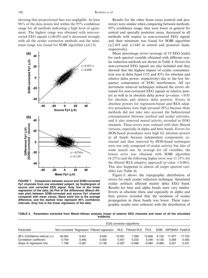
Figure 7 shows as an example the signal values forboth source and SOBI-corrected Fp1 channel in onesubject when applying Bland–Altman analysis. Fig-ure 7a indicated high similarity between signals(Pearson’s correlation coefficient = 0.899; and slope of

regression line = 0.921). Figure 7b shows the Bland–Altman plot with the differences of source minusSOBI-corrected Fp1 channel. According to this anal-ysis, bias (average of the differences) and precision(95% confidence ranges) were also calculated. Besides,regression was carried out in order to evaluate pro-portional biases.

Table 3 summarizes the following variables fromthe Bland–Altman analysis averaged for all subjectsand leads corresponding to the anterior brain region:95% confidence ranges, correlation coefficient andslope of regression line using both source and correctedEEG signals. The bias between source and correctedEEG data was almost zero (lower than 10-5) for allmethods so the constant bias was negligible for allmethods. Regarding the proportional bias, a highercorrelation coefficient and slope indicated a higherproportional bias: the higher values the higher differ-ences. In this case, bias is proportional to the magni-tude of the value due to high potentials of ocularcontamination. The highest slopes in magnitude areobtained with the non-corrected EEG signals. After-wards, regression, adaptive RLS, FastICA, and IN-FOMAX showed lower slopes and with not highcorrelation coefficients (lower than 0.492). Finally,slopes with values almost zero were obtained for theremainder ocular correction methods (filtered versionsof regression and adaptive RLS, PCA and SOBI)

TABLE 1. Pearson’s correlation coefficient for EOG correction procedures (mean of all the simulated subjects).

Area

EOG correction algorithms

Non-corrected Regression Filtered regression RLS Filtered RLS PCA SOBI INFOMAX FastICA

Anterior 0.385 0.740 0.881 0.730 0.871 0.640 0.909 0.782 0.675

Central 0.667 0.968 0.980 0.968 0.982 0.930 0.986 0.954 0.899

Posterior 0.851 0.989 0.992 0.988 0.993 0.976 0.993 0.986 0.965

All EEG channels 0.631 0.891 0.950 0.888 0.945 0.840 0.961 0.902 0.841

TABLE 2. Statistical increases between Pearson’s correlation coefficient for EOG correction procedures (paired t-tests were usedbetween Method A vs. Method B).

Method A

Method B

Non-corrected FastICA PCA RLS Regression INFOMAX Filtered RLS

Filtered

Regression

SOBI p < 0.001 p < 0.001 p < 0.001 p < 0.001 p < 0.001 p < 0.009 p < 0.013 p < 0.016

Filtered regression p < 0.001 p < 0.001 p < 0.001 p < 0.001 p < 0.001 p < 0.024 ns

Filtered RLS p < 0.001 p < 0.001 p < 0.001 p < 0.001 p < 0.001 p < 0.040

INFOMAX p < 0.001 p < 0.009 p < 0.012 ns ns

Regression p < 0.001 p < 0.005 p < 0.006 ns

RLS p < 0.001 p < 0.005 p < 0.006

PCA p < 0.001 ns

FastICA p < 0.001

Bold depicted p-value <0.01; Italicized p-value <0.05, and ns non-significative increases (mean of all EEG channels).

Ocular Reduction in EEG Signals 185

showing that proportional bias was negligible. At least96% of the data points lied within the 95% confidencerange for all methods indicating a high level of agree-ment. The highest range was obtained with non-cor-rected EEG signals (±46.05) and it decreased stronglywith all the ocular correction methods and the mini-mum range was found for SOBI algorithm (±6.15).

Results for the other brain areas (central and pos-terior) were similar when comparing between methods:95% confidence range, that were lower in general forcentral and specially posterior areas, decreased in allmethods with respect to non-corrected EEG signalsand their minimum was found for SOBI algorithm(±2.419 and ±1.643 in central and posterior leads,respectively).

Mean percentage errors (average of 19 EEG leads)for each spectral variable obtained with different ocu-lar reduction methods are shown in Table 4. Errors fornon-corrected EEG signals are also included and theyshowed that the highest impact of ocular contamina-tion was in delta band (152 and 45% for absolute andrelative delta power, respectively) due to the low fre-quency components of EOG interferences. All eyemovement removal techniques reduced the errors ob-tained for non-corrected EEG signals in relative pow-ers as well as in absolute delta power (p-values <0.01for absolute and relative delta powers). Errors inabsolute powers for regression-based and RLS adap-tive procedures were high (around 20%) because thesemethods did not take into account the bidirectionalcontamination between cerebral and ocular activities,and it also removed neural activity recorded in EOGchannels. These errors were reduced with their filteredversions, especially in alpha and beta bands. Errors forHOS-based procedures were high for absolute powersin all bands because independent components ex-tracted and then removed by HOS-based techniqueswere not only composed of ocular activity but also ofsome neural one. In average for all variables, thelowest error was obtained with SOBI algorithm(4.25%) and the following higher error was 11.33% forthe filtered RLS adaptive approach (p-value <0.001).This also happened in almost all target spectral vari-ables (see Table 4).

Figure 8 shows the topographic distribution oferrors for each ocular reduction technique. Simulatedocular artifacts affected mainly delta EEG band.Results for beta and alpha bands were very similar.Errors in absolute theta and especially in alpha andbeta powers revealed that the incidence of ocularpropagation in these bands was lower. These topo-graphic results were coherent with the distribution of

TABLE 3. Parameters extracted from Bland–Altman analysis (mean of anterior EEG channels and mean of all the simulatedsubjects).

Parameter

EOG correction algorithms

Non-corrected Regression Filtered regression RLS Filtered RLS PCA SOBI INFOMAX FastICA

95% Confidence interval (±) 46.054 9.641 6.646 10.061 7.260 12.836 6.152 11.977 17.723

Correlation coefficient 0.759 0.492 0.300 0.407 0.222 0.246 0.132 0.269 0.392

Slope of regression line 1.198 -0.381 -0.136 -0.307 -0.096 -0.084 -0.069 0.221 0.431

FIGURE 7. Comparison between source and SOBI-correctedFp1 channels from one simulated subject: (a) Scattergram ofsource and corrected EEG signal. Gray line is the linearregression of the data; (b) Plot of the differences (Bland–Alt-man plot) between SOBI-corrected and source Fp1 channelcompared with mean values. Black solid line is the averagedifference, and the dashed lines represent 95% confidenceintervals. Gray line is the linear regression of the data.

ROMERO et al.186

eye activity contamination across the scalp (seeFig. 2): errors were located at anterior sites andespecially in frontopolar and lateral–frontal regions.

SOBI algorithm provided the lowest errors betweenthe original cerebral sources and the corrected EEGsignals.

TABLE 4. Percentage errors (%) in spectral variables for EOG correction procedures (mean of all EEG channels and mean of allthe simulated subjects).

Spectral variables

EOG correction algorithms

Non-corrected Regression Filtered regression RLS Filtered RLS PCA SOBI INFOMAX FastICA

Total power 47.89 22.54* 11.17** 22.03* 10.56** 20.53* 4.32** 19.52* 43.04

ABS delta 151.78 19.86** 19.78** 18.57** 18.35** 18.83** 8.46** 29.89** 43.10**

ABS theta 3.78 20.39** 18.92** 20.32** 18.54** 22.41** 3.88 21.77** 53.97**

ABS alpha 0.98 24.91** 5.44** 24.77** 5.27** 22.54** 1.89* 13.46** 34.93**

ABS beta 0.87 22.06** 0.82** 22.19** 0.87 23.56** 4.39** 20.59** 67.97**

Mean ABS variables 41.06 21.95 11.23* 21.58 10.72* 21.57 4.59** 21.05 48.60

REL delta 45.24 9.93** 12.21** 10.29** 11.00** 11.47** 5.10** 9.07** 9.03**

REL theta 17.33 8.14* 10.69* 7.37** 10.84* 4.68** 3.17** 5.58** 8.71**

REL alpha 18.45 8.21** 9.47* 8.12** 8.98** 6.17** 3.47** 5.87** 7.75**

REL beta 18.50 14.41 18.64 12.59 17.52 6.73** 3.59** 6.47** 12.76

Mean REL variables 24.88 10.17** 12.75** 9.59** 12.09** 7.26** 3.83** 6.75** 9.56**

Mean all variables 33.87 16.72* 11.90** 16.25* 11.33** 15.21* 4.25** 14.69* 31.25

Statistical differences between errors for ocular correction methods and non-corrected signals were shown (* p < 0.05; ** p < 0.01).

FIGURE 8. Topographic maps of the errors (%) between the cerebral sources and the corrected EEG signals by using differentocular reduction techniques. Errors between sources and non-corrected (mixed) signals are included. Color key is discretized fromwhite to black in 10% stripes.

Ocular Reduction in EEG Signals 187

Real Data

Figure 9 shows as an example a 5-s epoch corre-sponding to real EOG and EEG signals displayed be-fore and after applying SOBI-based ocular correctionprocedure. Propagation of ocular contamination to thedifferent EEG leads and the bidirectional contamina-tion between ocular and cerebral activities can beobserved in the raw data (Fig. 9a). SOBI-baseddecomposition algorithm was performed using epochdurations of 15 s. The effects of ocular correctionprocedure on different EEG leads are shown inFig. 9b. By visual inspection, this example demon-strates that SOBI algorithm removed efficiently theocular artifacts from spontaneous real EEG data.

DISCUSSION AND CONCLUSION

Ocular artifacts in EEG data are a significant troublein the diagnosis of dysfunctional neural states and inthe evaluation of drug effects on the brain. Most usedtechniques to reduce them from spontaneous EEGsignals are based on regression analysis. Adaptive fil-tering is another approach also proposed for this pur-pose. Additionally, BSS procedures have been recentlyapplied in order to consider the mutual contaminationbetween cerebral and ocular activities. In this study for

BSS-based methods, an automated procedure usinglogical rules, which were based on spectral and topo-graphical information, was used in order to identifythose components related to eye activity. Quantitativecomparison of performance of these different ocularreduction methods required simulated signals whereocular and cerebral activities must be known a priori.

In this study, simulated EEG and EOG data wereobtained by means of real data recorded according tothe common procedure used in clinical routine. Forthis purpose, linear MISO models corresponding toocular and cerebral activity contaminations wereidentified by using an autoregressive structure withexogenous inputs. Although the same model orderswere used to cerebral and ocular contaminationsthrough the same medium which is the head, higherand different orders in both contamination could havebeen selected. However, the identification would notimprove sensitively because the FPE was not muchsmaller (see Fig. 1) and it is known that an unnecessarycomplex model could produce artifacts. It does notimply that ocular and cerebral propagations arefrequency dependent, a topic that has been questioned.Bioelectromagnetism considers that volume conduc-tion is instantaneous for frequencies lower than1000 Hz; in other words, frequency dependence ofocular propagation is negligible.23 It is yet to be

FIGURE 9. (a) Five second epoch of raw EOG and EEG signals containing prominent ocular artifacts. Some EEG channelscorresponding to left hemisphere are shown as an example; (b) Raw EOG and corrected EEG signals obtained after applyingautomatic SOBI-based ocular removal procedure.

ROMERO et al.188

definitively demonstrated whether ocular propagationis frequency dependent or independent. In fact, anyvolume conductor has both resistive and capacitiveproperties. Nevertheless, the detailed capacitive prop-erties of neocortex at the very low frequency compo-nents of most interest in EEG and EOG (0.5–20 Hz)have not been widely studied, but the available evi-dence suggests that capacitive effects have minimalinfluence on EEG volume conduction.24 On the otherhand, other studies have taken the assumption thatocular propagation exhibits frequency-dependentbehavior and apply techniques for artifact cancellationbased on filtered EOG signals.10,13,29,33

In this work, for ocular contamination, magnitudefrequency responses seemed to correspond to a lowpass filtering procedure (see Fig. 2). However, toanalyze them in more detail permitted to observe thatit was not exactly thus. In this way, 3-dB bandwidths(frequency at which the gain drops 3 dB) of these FIRfilters were calculated: 1.71 ± 0.76 Hz for vertical and3.11 ± 1.94 Hz for horizontal EOG in all channels.These bandwidths corresponded to the 96.67 ± 0.01and 97.76 ± 0.01% of the total energy of the verticaland horizontal EOG sources, respectively, for allsubjects and channels. Thus, almost whole ocularpropagation could be considered practically frequency-independent which was consistent to what would beexpected from biophysics knowledge. Regarding cere-bral activity contamination, the magnitude frequencyresponses from pre-frontal and lateral frontal sites toEOG locations (see Fig. 3) corresponded to quasi all-pass filters in the EEG frequency range and they couldbe approximated by constant propagation coefficients.Their filter gains showed a higher contamination in thevertical ocular channel than in the horizontal one.

Other studies that have been previously publishedcompared ocular reduction methods in simulated EEGsignals. However, the following approaches had notbeen compared so far: linear regression, adaptive fil-tering and BSS. Besides, filtered versions of the linearregression, which was already applied in Wallstromet al.,32 as well as of the adaptive filtering, which wassuggested but not applied in He et al.,13 were includedin this study. Additionally, performance of thesemethods was quantitatively evaluated by similaritybetween sources and corrected signals and by errors inthe spectral target variables used commonly in clinicalEEG studies.

Time and frequency results indicated that allmethodsreduced significantly the ocular contamination fromEEG data. However, corrected EEG signals fromfrontal regions showed that a partial neural componentwas also subtracted by regression, adaptive RLS- andPCA-based methods, possibly due to the mutual con-tamination between EEG and EOG signals (see Fig. 5).

This cerebral information removal was partly reduced inthe alpha and beta bands for regression and RLS tech-niques by applying a low-pass filter to EOG recordingsbefore subtraction. Other BSS procedures based on SOSor HOS found more appropriate, and not necessarilyorthogonal like PCA, source components. Assumptionsabout source modeling are different in SOS- and HOS-based algorithms: while SOS methods extract uncorre-lated sources, HOS-based techniques use statisticinformation (like higher-order cumulants, entropy ormaximum likelihood estimation) in order to obtainsources by minimizing an approximation of mutualinformation. Ocular sources extracted by HOS-basedalgorithms contained generally some cerebral activity,especially in anteriorly placed electrodes while it did nothappen with SOBI algorithm. Errors between spectralvariables for initial cerebral sources and corrected EEGsignals calculated with HOS-based algorithms de-creased when increasing data length, but they were farfrom the low errors obtained with some SOS-basedmethods (see Table 4: 31.25% for FastICA (n.s., whencompared to non-corrected errors) and 14.69% forINFOMAX (p< 0.015) compared to 4.25% for SOBI(p< 0.001), in average). Similar errors and correlationvalues were obtained for INFOMAX, regression andadaptive filtering methods. Topographic distributionsshowed that errors were located at anterior sites andespecially in frontopolar and lateral–frontal regions.Additionally, filtered version of linear regression andadaptive filtering provided good results in average:0.950 and 0.945 for Pearson’s correlation coefficients,and 11.90 and 11.33% for errors in spectral variables,respectively. However, correlation coefficients weremuch higher and errors much lower for SOBI algorithm(see Tables 1 and 4: 0.961 and 4.25% in average,respectively). Moreover, agreement level by 95% con-fidence ranges using Bland–Altman analysis was nar-rower for SOBI algorithm (see Table 3). This algorithmdid not show either constant or proportional bias.Consequently, this method showed much higher simi-larity between EEG sources and corrected EEG signals.

BSS-based approaches are based in some a-priorihypothesis: sources must be uncorrelated for SOS-based algorithms, and statistically independent forHOS-based ones. In the present paper, BSS techniqueswere used to separate ocular from cerebral activities inorder to eliminate the former. The fact that ocular andcerebral activities in a simulated subject came fromdifferent real subjects ensured the statistically inde-pendence between these activities. Additionally, in allcases, normalized correlations between each ocular(two) and each cerebral (19) sources were calculated.Results showed that correlation values were alwayslower than 0.023 indicating the fulfillment of thea-priori hypothesis of uncorrelatedness for SOS-based

Ocular Reduction in EEG Signals 189

methods. In the case of SOBI, a-posteriori correlationsbetween ocular activities and corrected-EEG signalswere calculated for each subject. Results showed valueslower than 0.062 indicating a poor level of correlation.Analogously, statistical independence was assessed bycalculating the normalized cross mutual information14

between ocular and cerebral sources. Cross mutualinformation quantifies the amount of informationgained about one signal from the measurement of asecond one. Normalized mutual information is zerowhen signals are independent, while it has a maximumvalue of one if both signals are identical. Resultsshowed values between ocular and cerebral sourceslower than 0.004 indicating that they were statisticallyindependent. Moreover, mutual information was alsocalculated between ocular activities and INFOMAX-based corrected EEG signals obtaining values alwayslower than 0.030.

Besides, these results can be considered another testof validation of the ocular reduction effectiveness: verylow values of correlation and mutual information be-tween ocular sources and corrected EEG signals en-sured that there were no relation between them andhence ocular contamination was efficiently removedfrom EEG data.

Thus, time and frequency results indicated thatSOBI algorithm reduced better the ocular artifactspreserving by far more cerebral activity (see Figs. 5and 8). This algorithm, that is simple, fast to computeand robust, presented the lowest errors in all leadsusing only short data segments of 15 s. Because HOS-based methods needed longer durations, sources wereless stationary which is one of the assumptions of BSS.Besides, SOBI algorithm used the temporal structureprovided by EOG and EEG data to achieve the sepa-ration. In this case, the use of additional well-definedsecond-order statistics (as covariances at different timelags) improved the estimation of the BSS model andthe separation of ocular and cerebral sources.

Finally, based on artificially generated both spon-taneous and corrupted EOG and EEG recordings, weconcluded that SOBI was the most effective and effi-cient techniques for eye movement reduction with re-spect to similarity between sources and corrected EEGsignals and to spectral target variables that are fre-quently used in a clinical real situation, even whenavailable data length was short.

ACKNOWLEDGMENT

This study was partially supported by CICYT(TEC2008-02754/TEC del Ministerio de Ciencia e In-novacion) from Spain.

REFERENCES

1Anderer, P., H. V. Semlitsch, B. Saletu, andM. J. Barbanoj.Artifact processing in topographic of electro-encephalo-graphic activity in neuropsychopharmacology. Psychiat.Res. 45:79–93, 1992. doi:10.1016/0925-4927(92)90002-L.2Barbati, G., C. Porcaro, F. Zappasodi, P. M. Rossini, andF. Tecchio. Optimization of an independent componentanalysis approach for artifact identification and removal inmagnetoencephalographic signals. Clin. Neurophysiol.115:1220–1232, 2004. doi:10.1016/j.clinph.2003.12.015.3Bell, A. J., and T. J. Sejnowski. An information maximi-zation approach to blind separation and blind deconvolu-tion. Neural. Comput. 7:1129–1159, 1995. doi:10.1162/neco.1995.7.6.1129.4Belouchrani, A., K. Abed-Meraim, J. F. Cardoso, and E.Moulines. A blind source separation technique using sec-ond-order statistics. IEEE Trans. Signal Process. 45:434–444, 1997. doi:10.1109/78.554307.5Bland, J. M., and D. G. Altman. Measurement error andcorrelation coefficients. Br. Med. J. 313:41–42, 1996.6Cichocki, A., S. Amari, K. Siwek, T. Tanaka, et al. ICA-LAB Toolboxes for Signal and Image Processing. Availablefrom http://www.bsp.brain.riken.jp/ICALAB/. Accessed10 March 2008.7Croft, R. J., and R. J. Barry. Removal of ocular artifactfrom the EEG: a review. Neurophysiol. Clin. 30:5–19, 2000.doi:10.1016/S0987-7053(00)00055-1.8Delorme, A., and S. Makeig. EEGLAB: an open sourcetoolbox for analysis of single-trial EEG dynamics includingindependent component analysis. J. Neurosci. Methods134:9–21, 2004. doi:10.1016/j.jneumeth.2003.10.009.9Delorme, A., T. Sejnowski, and S. Makeig. Enhanceddetection of artifacts in EEG data using higher-order sta-tistics and independent component analysis. Neuroimage34:1443–1449, 2007. doi:10.1016/j.neuroimage.2006.11.004.

10Gasser, T., L. Sroka, and J. Mocks. The transfer of EOGactivity into the EEG for eyes open and closed. Electro-encephalogr. Clin. Neurophysiol. 61:181–193, 1985.doi:10.1016/0013-4694(85)91058-2.

11Gasser, T., P. Ziegler, and F. Gattaz. The deleterious effectof ocular artifacts on the quantitative EEG, and a remedy.Eur. Arch. Psy. Clin. N. 241:241–252, 1992. doi:10.1007/BF02191960.

12He, P., G. Wilson, and C. Russell. Removal of ocularartifacts from electro-encephalography by adaptive filter-ing. Med. Biol. Eng. Comp. 42:407–412, 2004. doi:10.1007/BF02344717.

13He, P., G. Wilson, C. Russell, and M. Gerschutz. Removalof ocular artifacts from the EEG: a comparison betweentime-domain regression and adaptive filtering method usingsimulated data. Med. Biol. Eng. Comp. 45:495–503, 2007.doi:10.1007/s11517-007-0179-9.

14Hoyer, D., B. Pompe, K. H. Chon, H. Hardraht, C. Wi-cher, and U. Zwiener. Mutual information function as-sesses autonomic information flow of heart rate dynamicsat different time scales. IEEE Trans. Bio-Med. Eng. 52:584–592, 2005.

15Hyvarinen, A., and E. Oja. A fast fixed-point algorithm forindependent component analysis. Neural Comput. 9:1483–1492, 1997. doi:10.1162/neco.1997.9.7.1483.

16Hyvarinen, A., J. Karhunen, and E. Oja. IndependentComponentAnalysis. NewYork: JohnWiley&Sons, p. 481,2001.

ROMERO et al.190

17Jackson, L. B. FIR filter design techniques. In: DigitalFilters and Signal Processing, 3rd ed. Boston: KluwerAcademic Publishers, 1995, pp. 301–307.

18Jung, T.-P., S. Makeig, M. Westerfield, J. Townsend, E.Courchesne, and T. J. Sejnowski. Removal of eye activityartifacts from visual event-related potentials in normal andclinical subjects. Clin. Neurophysiol. 111:1745–1758, 2000.

19Kierkels, J. J. M., G. J. M. van Boxtel, and L. L. M.Vogten. A model-based objective evaluation of eye move-ment correction in EEG recordings. IEEE Trans. Bio-Med.Eng. 53:246–253, 2006.

20Lins, O. G., T. W. Picton, P. Berg, and M. Scherg. Ocularartifacts in recording EEGs and event-related potentials II:source dipoles and source components. Brain Topogr. 6:65–78, 1993. doi:10.1007/BF01234128.

21Ljung, L. System Identification—Theory for the User. 2nded.Upper SaddleRiver,NJ: PTRPrenticeHall, p. 609, 1999.

22Makeig, S., A. J. Bell, T.-P. Jung, and T. J. Sejnowski.Independent component analysis of electro-encephalo-graphic data.Adv.Neural Inf. Process. Syst. 8:145–151, 1996.

23Malmivuo, J., and R. Plonsey. Volume source and volumeconductor. In: Bioelectromagnetism. Principles andApplications of Bioelectric and Biomagnetic Fields. NewYork: Oxford University Press, 1995, pp. 133–147.

24Nunez, P. L., and R. Srinivasan. Electric Fields of theBrain. 2nd ed. New York: Oxford University Press, 2006.

25Romero, S., M. A. Mananas, and M. J. Barbanoj. Acomparative study of automatic techniques for ocularartifact reduction in spontaneous EEG signals based onclinical target variables: a simulation case. Comput. Biol.Med. 38:348–360, 2008. doi:10.1016/j.compbiomed.2007.12.001.

26Saletu, B., P. Anderer, K. Kinsperger, and J. Grunberger.Topographic brain mapping of EEG in neuropsychophar-macology—Part II. Clinical applications (pharmaco EEGmapping). Meth. Find. Exp. Clin. Pharmacol. 9:385–408,1987.

27Schlogl, A., C. Keinrath, D. Zimmermann, R. Scherer, R.Leeb, and G. Pfurtscheller. A fully automated correctionmethod of EOG artifacts in EEG recordings. Clin. Neuro-phyiol. 118:98–104, 2007. doi:10.1016/j.clinph.2006.09.003.

28Semlitsch, H. W., P. Anderer, P. Schuster, and O. Presslich.A solution for reliable and valid reduction of ocular arti-facts applied to the P300 ERP. Psychophysiology 23:695–703, 1986. doi:10.1111/j.1469-8986.1986.tb00696.x.

29Sornmo, L., and P. Laguna. EEG signal processing. In:Bioelectrical Signal Processing in Cardiac and NeurologicalApplications. Elsevier Academic Press, 2005, pp. 55–180.

30Vasegui, S. V. Adaptive filters. In: Advanced Digital SignalProcessing and Noise Reduction, 2nd ed. Chichester: JohnWiley & Sons, 2000.

31Vigario, R. N. Extraction of ocular artifacts from EEGusing independent component analysis. Electroencephalogr.Clin. Neurophysiol. 103:395–404, 1997. doi:10.1016/S0013-4694(97)00042-8.

32Wallstrom, G. L., R. E. Kass, A. Miller, J. F. Cohn, and A.F. Nathan. Automatic correction of ocular artifacts in theEEG: a comparison of regression-based and component-based methods. Int. J. Psychophysiol. 53:105–119, 2004.doi:10.1016/j.ijpsycho.2004.03.007.

33Woestenburg, J. C., M. N. Verbaten, and J. L. Slanger. Theremoval of eye-movement artifact from the EEG byregression analysis in the frequency domain. Biol. Psychol.16:127–147, 1983. doi:10.1016/0301-0511(83)90059-5.

Ocular Reduction in EEG Signals 191