arX

iv:q

uant

-ph/

0012

091v

1 1

8 D

ec 2

000

NONLOCAL EFFECTS OF PARTIAL MEASUREMENTS

AND QUANTUM ERASURE

Avshalom C. Elitzur∗

Unit of Interdisciplinary Studies, Bar-Ilan University, 52900 Ramat-Gan, Israel.

and

The Bhaktivedanta Institute, Juhu, Juhu Road, Mumbai 400049, India.

Shahar Dolev†

The Kohn Institute for the History and Philosophy of Sciences,

Tel-Aviv University, 69978 Tel-Aviv, Israel.

(February 1, 2008)

Partial measurement turns the initial superposition not into a definite outcome but into a greater

probability for it. The probability can approach 100%, yet the measurement can undergo complete

quantum erasure. In the EPR setting, we prove that i) every partial measurement nonlocally creates

the same partial change in the distant particle; and ii) every erasure inflicts the same erasure on

the distant particle’s state. This enables an EPR experiment where the nonlocal effect does not

vanish after a single measurement but keeps “traveling” back and forth between particles. We study

an experiment in which two distant particles are subjected to interferometry with a partial “which

path” measurement. Such a measurement causes a variable amount of correlation between the

particles. A new inequality is formulated for same-angle polarizations, extending Bell’s inequality

for different angles. The resulting nonlocality proof is highly visualizable, as it rests entirely on

the interference effect. Partial measurement also gives rise to a new form of entanglement, where

the particles manifest correlations of multiple polarization directions. Another novelty in that the

measurement to be erased is fully observable, in contrast to prevailing erasure techniques where it

can never be observed. Some profound conceptual implications of our experiment are briefly pointed

out.

PACS numbers: 03.65.Bz, 03.67.*

∗email: cfeli@weizmann.weizmann.ac.il†email: shahar dolev@email.com

0

INTRODUCTION

Bell’s theorem [1] has made it possible, for the first

time, to experimentally demonstrate quantum nonlocal-

ity. Later, the GHZ experiment [2] and Hardy’s [3] proof

without inequalities extended the proof to new domains.

All these proofs, however, involve complete measure-

ments. This is insufficient since, at the quantum level,

measurement can be a continuous process, the interme-

diate stages of which have seldom been studied.

Is it possible to prove that nonlocal effects are pro-

duced even by small stages of the measurement process?

Moreover, is it possible to show that nonlocal effects are

formed not only by measurement but also by the time-

reversed process, namely, quantum erasure? Affirmative

answers would render nonlocality much more intriguing

because, in the ordinary EPR experiments, a single mea-

surement of a particle disentangles it, and no further

measurements can reveal nonlocal effects. Once, how-

ever, the above two questions are answered in the affir-

mative, nonlocality will turn out to connect not only dis-

crete events but continuous processes as well. The non-

local influence will then appear to “bounce” back and

forth, many times, between the distant particles during

the measurements. Several other intriguing features of

QM, such as reversibility and information capacity, would

also become manifest.

The organization of this article is as follows. Sec-

tion I introduces interaction-free measurement. Section

II shows how, when the wave function is appropriately

split, interaction-free measurement becomes partial. Sec-

tion III shows that such a measurement obeys the un-

certainty relations in that it partially disrupts a non-

commuting variable. Section IV shows that partial mea-

surement(PM) can sometimes be completely reversed.

Section V presents a hybrid, EPR-PM experiment in or-

der to show that partial measurement and its erasure

exhibit nonlocal effects. Section VI shows that quan-

tum theory’s predictions for this experiment quantita-

tively differ from those of a local theory. In Section VII

a Bell-like inequality is shown to break by the EPR-PM

experiment. Section VIII studies the case of a multiple

partial measurement on one particle and its unique non-

local consequences. Section IX discusses the novel form

ΨΨ xpBS

x

Mirror

��FIG. 1. It is possible to restore photon’s exact state as

long as no measurement is performed.

of quantum erasure made possible by our experiment.

Section X points out some bearings of these findings on

quantum theory.

I. INTERACTION-FREE MEASUREMENT AND

THE UNCERTAINTY RELATIONS

Single-particle interferometry provides some of the

most intriguing illustrations for quantum-mechanical

principles, and in recent years it has become technically

feasible. Consider a photon entering a calcite crystal po-

sitioned to divert the incident photon according to its

polarization along the x axis (Fig. 1). If the photon’s po-

larization is 90◦ (Px = +1, |↑〉), it will be diverted to the

lower path, whereas if it is 0◦ (Px = −1, |→〉) it will be

diverted to the upper path. The calcite thus acts as a po-

larizing beam splitter (pBS), similar to the Stern-Gerlach

magnet for spin-1/2 particles. As long as no measurement

has been made to find out which path the photon took –

thereby leaving the photon’s polarization undetermined

too – the photon will remain in a superposition of both

paths and both polarizations:

|Ψ〉 = c1 |↑〉 + c2 |→〉. (1)

So far, the splitting of the wave function is reversible. A

second calcite, aligned at the x plane as the first but fac-

ing an opposite direction (denoted by x), re-unites the re-

sulting |↑〉 and |→〉 beams, so that the photon re-emerges

in one single beam, in the same state as it has entered

the first calcite (Fig. 1).

The reversibility of splitting the photon along the x di-

rection is demonstrated by the measurement of another,

noncommuting variable. Before splitting, let the photon

impinge on a calcite positioned in 45◦ to the x direc-

tion, measuring its y polarization. Suppose that the y

1

Ψ

xx

y

y��� �FIG. 2. As long as no measurement is taken to tell the

photon’s polarization in the x direction, its polarization along

the y direction remains intact.

polarization has been found to be +45◦ (Py = +1, |ր〉).Then, let the photon split according to its x polarization

and re-unite again (Fig. 2). If no measurement has been

made between the splitting and re-uniting, we are left ig-

norant about the photon’s x polarization. Consequently,

the y polarization will remain intact: a final y measure-

ment will always yield a polarization of +45◦, just like

the initial y measurement.

Suppose, however, that two detectors are placed on the

two routes of the split wave function prior to its reuni-

fication (to enable the later reunification of the rays, let

the measurements be of the non-demolition type, such

that the detectors do not absorb the photon in case of

detection). Since the |ր〉 state is an even mixture of |→〉and |↑〉,

|ր〉 =1√2(|↑〉+ |→〉), (2)

in 50% of the cases the upper detector will click, and

in the other 50% the lower one will. This measurement

has an irreversible consequence: The knowledge we have

gained about the photon’s polarization will takes the cost

of blurring the other, non-commuting variable, obeying

an uncertainty relation of the form:

∆Px · ∆Py ≥ 2i[Px, Py]. (3)

Fig. 3 demonstrates this principle. Once Px is ascer-

tained, Py is disrupted; a second y measurement will yield

either +45◦ (|ր〉) or −45◦ (|ց〉), randomly. This is sim-

ilar to the ordinary interference effect in a Mach-Zender

Interferometer (MZI), where obtaining which-path infor-

mation disrupts the photon’s initial momentum.

Here a peculiar possibility emerges: What happens if,

in order to measure Px, we place only one detector on

Ψ

xx

Detectory

y��� ��FIG. 3. A measurement that discloses the photon’s x

polarization destroys the y polarization even when the mea-

surement has been carried out by a single detector that did

not click.

one of the two routes? If the detector clicks, the an-

swer is clear: This is an ordinary measurement, hence

we should observe the above disruption of Py. The situa-

tion becomes more intriguing in the remaining 50% of the

cases, when the single detector clicks not. Although no

observable interaction has taken place, the very silence

of the detector indicates that the photon has traversed

the other path, thereby disclosing the photon’s polariza-

tion with certainty. Hence, Py should be disrupted in

this case too, just because the silent detector could have

clicked!

This “interaction free measurement” [4] has been the

subject of intense experimental and theoretical study in

the last few years [5–7](see [8] for a comprehensive re-

view). In the present context, it has two unique features

that warrant attention. First, with a simple modification,

interaction-free measurement can be partial, leaving the

wave function in a certain degree of superposition even

after the measurement. Second, it can be completely re-

versed.

II. MEASUREMENT CAN BE PARTIAL

Nearly always, measurement is regarded as a single

event, whereby the superposition of all possible states

gives its place to one state. In reality, however, there can

be many intermediate stages in the measurement process,

stages that only change the initial probabilities without

yet giving a definite result. [9–12]

Following is a simple apparatus for partial measure-

ments. Let a photon be split by a calcite in the above

manner. Next, with the aid of many partly-silvered mir-

rors, let the |↑〉 beam split further into 100 beams. The

2

Detector

100

4

3

2

1

1%

1%

1%

1%

1%

Ψ

x

y �

pBSx

�pBS�

pBSx

x ypBS

�Partiallysilveredmirrors

FIG. 4. A series of partly-silvered mirrors splits each half of the wave function into 100 equal beams. Here too, as long as

no measurement has been taken on any of the 200 beams, the y polarization remains intact.

transmission coefficients of the mirrors are graded such

that all the 100 beams have an equal intensity of 1% of

the original beam (Fig. 4). The first mirror transmits99100 of the incident beam, the second 98

99 and so on, with

the 99th mirror transmitting 1/2 of the beam, and the

last one being a solid mirror. Similarly, let the |→〉 beam

split into another 100 by the same technique. The pho-

ton is now in a superposition of 200 beams, such that, if

its polarization along the x direction is 90◦ it might be

detected in one out of the lower 100 beams, whereas if

its polarization is 0◦ it might be detected in one out of

the 100 upper beams.

Finally, let a complementary series of mirrors re-unite

all 200 beams into two |↑〉 and |→〉 beams, and let a re-

3

versed x calcite re-unite the resulting beams. The appa-

ratus keeps the paths of all the beams in the same length,

so as to keep the beams in phase.∗ This way, the entire

splitting process is reversed and the photon re-emerges

as one single beam.

Here too, we can demonstrate the superposition of the

photon’s x polarization by performing two y polarization

measurements, one before and one after the splitting and

re-unification processes.

As long as no measurement is performed, the superpo-

sition will remain intact and all the photon will always

emerge in the same state as it entered the apparatus, e.g.,

|ր〉 as in Fig. 4.

This setup enables performing partial measurements.

We can now remove one of the mirrors and place a detec-

tor, as demonstrated on the third beam of the |↑〉 branch

of Fig. 4. If the detector clicks, we know for certain that

the photon’s polarization is |↑〉 and the measurement is

complete. In 99.5% of the cases, however, the detector

will not click. This constitutes an interaction-free mea-

surement, which should alter the wave function. Yet,

since the portion of the wave function thus measured is

so tiny, the superposition will change only slightly,

|ր〉 =1√2(|↑〉+ |→〉) −→

√

99

199|↑〉 +

√

100

199|→〉, (4)

and will continue slightly changing for each further mea-

surement on the remaining beams that yields no click. In

other words, each interaction-free measurement slightly

reduces the probability that the photon’s polarization is

|↑〉, thereby increasing its probability to have a |→〉 po-

larization. For n detectors on the 90◦ branch, the effect

on the wave-function will be

1√2(|↑〉+ |→〉)

−→√

100 − n

200 − n|↑〉 +

√

100

200 − n|→〉

=

√

α

1 + α|↑〉 +

√

1

1 + α|→〉, (5)

∗This is, essentially, a modification of the Mach-Zender in-

terferometer. Aligning these mirrors to about one wavelength

error is a difficult task, but completely possible in current

technology.

where α is the intensity of the (unmeasured) |↑〉 beam:

α =100− n

100. (6)

Let us denote the operator of partial polarization mea-

surement in the x up direction with intensity α as:

Partial Polarization Measurement ≡ P↑α. (7)

(Note again that α is the unmeasured intensity).

This operator obeys the following multiplication law:

P↑β · P↑α = P↑α·β . (8)

A familiar question, central to quantum theory, now

poses itself: Does partial measurement change merely

our knowledge about the photon or is this a real physi-

cal change going on with the photon’s state? Interaction-

free measurement provides a straightforward way to show

that the latter is true.

Recall that, prior to the photon’s splitting along the x

direction, its polarization has been measured along the y

direction and was found to be |ր〉. All one has to do now

is to reunite the |↑〉 and the |→〉 beams, and then mea-

sure again the y polarization. If no attempt has been

made to determine which of the 200 paths the photon

took in the x direction, the photon will emerge from the

interferometer with its x polarization unmeasured, hence

its y polarization will remain |ր〉 with 100% certainty.

If, however, a measurement has been made to find out

the photon’s x polarization, this measurement will have

a proportionate effect. If one of the detectors click, then

the measurement is complete and the photon’s y polar-

ization will be totally disrupted, as in Fig. 3. But if the

measurement is interaction-free – i.e., a few beams mea-

sured with no click – the y polarization will be only partly

disrupted (see also Ref. [9]). Instead of a pure |ր〉 state,

we will have:

|Ψα〉 ≡ P↑α |Ψ〉

=

√

α

1 + α|↑〉 +

√

1

1 + α|→〉

=1 +

√α√

2 + 2α|ր〉 +

1 −√α√

2 + 2α|ց〉. (9)

This change of the wave function is an objective, phys-

ical event. Measuring the photon’s y polarization before

and after the partial measurement will show that, at the

4

0.800.60

0.40

0.10

0.20

0.60

0.40

0.20

1.00

0.10

0

0.2

0.4

0.6

0.8

1

0 0.2 0.4 0.6 0.8 1

Normalized

Non-normalized

Polarization plane withno measurementθ=45o

θ

α

Ψ

�

�

Ψ

Polarization plane withα=0.10, normalized Ψ

Polarization plane withα=0.10, while regardingmeasurements withinteraction.

Chart 1. The polarization angle as a function of α.

statistical level, the y polarization has been disrupted

proportionately to the knowledge we gained about the x

polarization.

III. PARTIAL MEASUREMENT EXERTS A

PARTIAL EFFECT ON NON-COMMUTING

VARIABLES

Let us now turn to the way partial measurement obeys

the uncertainty principle. The effect of a partial measure-

ment of Px on Py can be regarded as a rotation of the

polarization plane: Drawing a vector with the |→〉 com-

ponent as the x ordinate and the |↑〉 component as the

y ordinate, will give θ = tan−1(

〈↑|Ψα〉〈→|Ψα〉

)

as the angle of

the polarization plane. The initial state of |ր〉 has two

equal components of the x polarization, namely, |→〉 and

|↑〉, resulting in θ = 45◦. When a partial Px measure-

ment is taken, the |↑〉 component diminishes while the

|→〉 component increases, causing the polarization plane

to rotate clockwise, until a complete measurement gives

a pure |→〉 state (Chart 1).

Chart 1 also allows us to look at the vectors without

normalizing Ψ for ‖ |Ψα〉‖2 = 1: The formulation given

in Eq. (9) keeps the polarization vectors normalized since

it counts only the cases where |ր〉 or |ց〉 were measured

– excluding all the cases where a complete measurement

took place and ended up with a click in one of the |↑〉detectors. An efficient way to look at the wave-function

is to keep track of these |↑〉 measurements. In this case,

the probabilities for |ր〉 and |ց〉 will not sum to 1, and

the vector in Chart 1 will get shorter as α diminishes.

Formally:

|Ψ′α〉 =

√

α

2|↑〉 +

√

1

2|→〉

=1 +

√α

2|ր〉 +

1 −√α

2|ց〉. (10)

This fact will turn out to be important later.

We can now calculate the correlation coefficient be-

tween the initial and the final y polarizations as a func-

tion of the magnitude of the partial measurement:

Cy(α) =∥

∥〈ր|Ψα〉∥

∥

2=

(

1 +√

α√2 + 2α

)2

. (11)

Cy(α) ranges from 1 (when a total correlation is kept) to

0.5 (when we have no correlation at all, since there is

5

0

0.2

0.4

0.6

0.8

1

0 0.2 0.4 0.6 0.8 1

∆Px

∆Py

∆P

α

Chart 2. ∆Px and ∆Py as a function of α.

an equal probability to find |ր〉 or |ց〉). For example,

if measurements have been carried out on 50 out of the

100 |↑〉 beams, yielding no click, then α = 0.5 and the

agreement between the y polarization before and after

the Px measurement will be:

Cy(α) =( 1 +

√α√

2 + 2α

)2

≃ 97%.

Indeed, since the x and y polarization directions are non-

commuting variables, they satisfy the uncertainty rela-

tions mentioned in Eq. (3), and when applied to the above

case of partial measurement,

∆Px =2√

α

1 + α, ∆Py =

1 − α

1 + α, (12)

which vary with α as in Chart 2.

It is easily seen that as α increases (that is, fewer mea-

surements on the |↑〉 branch), ∆Px also increases and

∆Py decreases. That means that the more we measure

on the |↑〉 branch, the more precise knowledge we gain

about Px (hence ∆Px decreases), and the more knowl-

edge we lose about Py (hence ∆Py increases).

IV. PARTIAL MEASUREMENT IS AMENABLE

TO COMPLETE ERASURE

An intriguing peculiarity of partial measurement is

that, in contrast to the ordinary one, it can sometimes

be totally reversed. To do this, there is no need to time-

reverse the operation of any detector; one can merely

repeat the partial measurement on the photon’s opposite

branch (Fig. 5).

For example, let n detectors be placed on n paths of a

photon’s |↑〉 branch. On average, in 200−n200 of the cases,

these detectors will not click. This is a partial measure-

ment, its outcome being given by Eq. (5). Now let an-

other battery of n detectors be placed on n paths of the

same photon’s |→〉 branch. On average, in 200−2n200 of the

cases, none of these detectors will produce a click either.

This will completely undo the measurement and turn the

wave-function back to the initial superposition:

1√2

(|↑〉+ |→〉) −→

Measurement

−→√

100 − n

200 − n|↑〉 +

√

100

200 − n|→〉

=

√

α

1 + α|↑〉 +

√

1

1 + α|→〉 −→

Erasure

−→√

100 − n

200 − 2n|↑〉 +

√

100 − n

200 − 2n|→〉

=1√2

(|↑〉+ |→〉) . (13)

According to the notation we used for the partial mea-

surement, the erasure process will take the form:

P→α · P↑α = 1. (14)

This reversal occurs when the two partial measurements

on the opposing branches are of the same magnitude. In

6

Ψ

x

y

��� x y �

FIG. 5. When the same number of paths is interaction-freely measured on both the |→〉 and |↑〉 branches, their overall

effects cancel each other and the photon returns to the original superposition.

the more general case, of placing n detectors on the |↑〉branch and m detectors on the |→〉 branch, the corre-

lation (or rather the mismatch) between the initial and

final Py measurement will be:

|Ψαβ〉 ≡ P→β · P↑α |Ψ〉

=

√

α

β + α|↑〉 +

√

β

β + α|→〉

=

√β +

√α√

2β + 2α|ր〉 +

√β −√

α√2β + 2α

|ց〉, (15)

with correlation coefficient:

Cy(αβ) =

(√α +

√β√

2α + 2β

)2

=

(

1 +√

k√2 + 2k

)2

, (16)

7

where α and β are the beam intensities of the |→〉 and

the |↑〉 branches, respectively, and k is the ratio between

them:

α =100 − n

100, β =

100 − m

100, k =

α

β. (17)

Notice that Cy(αβ) depends on the ratio k alone. That

means, for example, that a measurement of 50% of the

|↑〉 branch (k = 1√2) will yield exactly the same Cy(αβ)

as a measurement of 90% of the |↑〉 branch and 80% of

the |→〉 branch, or 99% of the |↑〉 branch and 98% of the

|→〉 branch, etc. In other words, the exact number of

paths on either branch does not matter, nor does their

relative intensities, nor the number, nor the identity of

the measured paths. The only thing that counts is the

ratio of the unmeasured parts of the two branches!

P→β · P↑α = P↑α/β . (18)

Consequently, the partial measurement operators in the

x direction are commutative:

P→β · P↑α = P↑α · P→β = P↑α/β = P→β/α. (19)

This ratio looks natural when discussing a single pho-

ton, as interference is known to depend on the intensities

of the various beams diverging and re-converging from

the initial wave function. Later, however, this ratio will

prove to be of crucial significance as a proof for nonlocal

influence between distant photons.

An important feature of the erasure process is that it

complies with the “no free lunch” principle. Any mea-

surement on the |→〉 path to restore the exact |ր〉 state

will also diminish an equal part of the |↑〉 part, as seen

in Fig. 6. To trace the cost of the erasure, we must keep

track of the measured portion of the beam, hence a for-

mulation similar to Eq. (10) is used with the inclusion of

the erasure process:

|Ψ′αβ〉 =

√

α

2|↑〉 +

√

β

2|→〉

=

√β +

√α

2|ր〉 +

√β −√

α

2|ց〉. (20)

�� �

�

(a) Initial setup: |Ψ〉 =|ր〉.

�� �

�Rotation

(b) A partial measurement on the |↑〉 branch rotates the

polarization plane: |ր〉 diminishes while |ց〉 increases.

�

�Rotation

(c) Following a counter-measurement on the |→〉 branch, the

initial state is restored. The |ց〉 part is nullified but |ր〉

diminishes too.

FIG. 6. The cost of undoing a measurement.

8

Let us now summarize Sections II-IV: The splitting of

the wave function into 200 paths enables carrying out a

partial measurement, whose effect is manifested by the

proportionate disruption of the interference effect. This

setup also allows, in some cases, a complete erasure of

the partial measurement and consequently a restoration

of the interference pattern.

V. NONLOCAL EFFECTS OF PARTIAL

MEASUREMENT AND ERASURE, REVEALED

BY INTERFEROMETRY

Is it possible to show that such a partial measurement

has nonlocal effects? Our proof involves an experiment

with two particles in a singlet state. We show that, when

both photons are subjected to interferometry, the partial

measurement and erasure performed on each photon dis-

rupt and restore, respectively, the interference effects of

both photons.†

Consider, then, a pair of spacelike-separated photons,

A and B, in an entangled state, each entering an appa-

ratus of the form described in Fig. 4. This is a hybrid

EPR-PM experiment (Fig. 7). If both Px polarization

are measured, they will be 100% correlated but the Py

polarizations will be unrelated. Conversely, if no detec-

tion is performed to find out which of the possible 200

paths any of the photons has taken, their x polarization

will remain unmeasured, hence their Py correlations will

remain intact.

Now let some detectors be placed on n out of the 100

paths of the |↑〉 branch of photon A. Photon B, in con-

trast, will not undergo any measurement of Px, only of

its Py.

In 200−n200 of the cases, all detectors measuring photon A

will perform an interaction-free measurement, changing

the wave function as in Eq. (9). But here, due to the

singlet state connecting the two photons, a unique state

evolves. The partial measurement has partly disrupted

the two photons’ EPR entanglement:

†For combining IFM and EPR experiments to prove the non-

local nature of the former, see [13,14].

|EPR〉 =1√2

(|↑〉1 |↑〉2+ |→〉1 |→〉2)

−→√

100 − n

200 − n|↑〉1 |↑〉2 +

√

100

200 − n|→〉1 |→〉2

=

√

α

1 + α|↑〉1 |↑〉2 +

√

1

1 + α|→〉1 |→〉2, (21)

where α, again, is the intensity of the beam (as in Eq.

(6)). This change causes a decrease in the correlation

between their y polarizations:

|Ψα〉 ≡ P↑1α |Ψ〉

=

√

α

1 + α|↑〉1 |↑〉2 +

√

1

1 + α|→〉1 |→〉2

=1 +

√α

2√

1 + α(|ր〉1 |ր〉2+ |ց〉1 |ց〉2)

+1 −√

α

2√

1 + α(|ր〉1 |ց〉2+ |ց〉1 |ր〉2)

=1 +

√α√

2 + 2α|EPR〉 +

1 −√α√

2 + 2α|EPR〉. (22)

where |EPR〉 is the “anti-EPR” state in which the pho-

tons are entangled, but in reverse polarization:

|EPR〉 =1√2

(|ր〉1 |ց〉2+ |ց〉1 |ր〉2) . (23)

As we can see, the partial measurement did not break

the entanglement between the two photons. Instead, the

pure EPR state became “contaminated” by a certain

amount of the anti-EPR state. This means that mea-

surements of the y polarization of photons A and B have

a probability of(

1+√

α√2+2α

)2

to yield correlated results, and

a probability of(

1−√α√

2+2α

)2

to yield opposite results. The

latter probability will grow as the magnitude of the par-

tial measurements on Px grows (that is, as α diminishes)

until the correlation drops to the random level of 50%-

50% as α drops to 0 in case of a complete measurement

(Chart 3).

As we will show below, the fact that the photons re-

main entangled even after partial measurement was per-

formed enables us to increase or decrease the amount of

the anti-EPR component in subsequent measurements.

Our next aim is to show that such a reversal can erase

not only the outcome of a measurement performed on the

same photon, but also that of the other photon. Consider

the erasure of a partial measurement as described in Sec-

tion II. If the erasure works, i.e., the measurement of the

9

x y x

� � � �

EPRSource

Photon A

x y x

� � � �

Photon B

FIG. 7. An EPR-interferometry experiment. As long as no measurement of the two photons’ x polarizations is made, their

final y polarization will be 100% correlated. When partial Px measurements are carried out, the changes in the correlation

between their y polarizations can demonstrate their nonlocal effects.

opposing branch also turns out to be interaction-free, the

correlation between the two photons’ y polarizations will

be restored:

|Ψαβ〉 ≡ P→1β · P↑1α |Ψ〉=

√

α

α + β|↑〉1 |↑〉2 +

√

β

α + β|→〉1 |→〉2

10

=

√β +

√α

2√

α + β(|ր〉1 |ր〉2+ |ց〉1 |ց〉2)

+

√β −√

α

2√

α + β(|ր〉1 |ց〉2+ |ց〉1 |ր〉2)

=

√β +

√α√

2α + 2β|EPR〉 +

√β −√

α√2α + 2β

|EPR〉. (24)

Where β is the intensity of the |→〉 branch, as in Eq.

(17).

It is now clear that when α = β, the | EPR〉 part

diminishes and the final state is the original |EPR〉 state,

restoring the initial entanglement of photons A and B.

Note that the restoration process is reminiscent of

a procedure proposed by Deutsch et al. [15] for “en-

tanglement purification” of EPR-like pairs. However,

their procedure suffers from lack of information about

the partially-entangled state. Consequently, it necessi-

tates destroying every other transmitted particle, which

serves as “entanglement-control” particle, and then de-

stroying also the accompanying particle, should the

“entanglement-control” particle indicate a non-entangled

state. Our experiment, in contrast, does not require

“testing” the particles for entanglement. Each and ev-

ery particle that is being “caught” by the detector in

the “counter-measurement” is a non-entangled particle.

Magically the QM formalism ensures that only the non-

entangled particles will be caught by the detector! ‡

Therefore, when partial measurements and erasures

are performed on two entangled photons, the local and

nonlocal interpretations markedly differ:

Local Argument A: § Both the disruption of the cor-

relation and its restoration are performed only by

photon A’s local interaction with the nearby detec-

tor, without affecting photon B whatsoever.

Nonlocal refutation: The correlation between the two

y polarizations will be restored even if we perform

‡This point will be elaborated on Section VI.§Proving nonlocal action is always difficult as adherents of

locality often come up with very awkward yet not-impossible

local mechanisms. Disproving such mechanisms is a tedious

task,yet essential for a proof’s completion. We therefore con-

sider and disprove here all possible localist arguments.

the partial x measurement on photon A and the un-

doing of this measurement on photon B.

Here is the proof. Let γ and δ denote the intensities

of the |→〉 and |↑〉 branches of photon B, respectively. If

both photons are subjected to partial measurements, the

pair’s state will be:

|Ψαβγδ〉 ≡ P→2δ · P↑2γ · P→1β · P↑1α |Ψ〉 (25)

=

√

αγ

αγ + βδ|↑〉1 |↑〉2 +

√

βδ

αγ + βδ|→〉1 |→〉2

=

√βδ +

√αγ√

2αγ + 2βδ|EPR〉 +

√βδ −√

αγ√2αγ + 2βδ

|EPR〉.

Again, the entanglement between the photons is kept

(though evolving into the unique state similar to Eq.

(23)), and the correlation between the photons’ y po-

larizations would be:

Cy(αβγδ) = ‖〈EPR |Ψαβγδ〉‖2

=

(√

βδ +√

αγ√2αγ + 2βδ

)2

=

(

1 +√

K√2 + 2K

)2

, (26)

where, again, α and β are, respectively, the beam inten-

sities of the |→〉 and the |↑〉 branches of photon A, and

γ and δ are the |→〉 and |↑〉 branches of photon B. K is

the ratio between the intensities of the two photons:

K =βδ

αγ. (27)

A few points are worth mentioning here:

1. The |EPR〉 component will always be greater than

or equal to the |EPR〉 part. Hence, in the above

setup, one can never reach a situation when the two

photons are manifestly anti-correlated.

2. In the extreme case when either α, δ, β, or γ

equals 0 (that is, a complete measurement was

performed), the resultant state is an even blend

of |EPR〉 and |EPR〉 states, and Cy(αβγδ) = 12 .

That means that, following a complete measure-

ment of Px on one photon, no information can be

obtained about the other’s y polarization, as there

are even probabilities to find the other photon in

the same polarization (|EPR〉) or in the opposite

one (|EPR〉).

11

0.0

0.2

0.4

0.6

0.8

1.0

0.000.200.400.600.801.00

EPR

anti-EPR

α

Chart 3. EPR and anti-EPR parts as a function of α.

3. The opposite extreme case occurs when αδ = βγ,

thereby Cy(αβγδ) = 1. Then, the two photons will

restore the original |EPR〉 state of 100% entangle-

ment.

4. The process of “erasing” the measurement bears a

cost: Getting rid of the anti-EPR component will

take the toll of diminishing the EPR part in equal

amount. That means that many measurements will

end up with a click. In order to measure this effect,

we have to rewrite Eq. (25) without normalization

for ‖Ψ‖2 = 1 after each measurement (as we did

before in Eqs. (10) and (20)). When keeping |Ψ〉relative to it’s initial intensity (where α = β = γ =

δ = 1), we get:

|Ψ′αβγδ〉 =

√βδ +

√αγ

2|EPR〉

+

√βδ −√

αγ

2|EPR〉. (28)

Now, for example, if a measurement of 50% was

taken on α, the result will be:

|Ψ′1〉 =

1 +√

1/22

|EPR〉 +1 −

√

1/22

|EPR〉,

(29)

whereas after a counter-measurement of 50% on β

or δ, the result will be:

|Ψ′2〉 =

1

2|EPR〉. (30)

Hence erasing the anti-EPR part took the toll of an-

other reduction of 1√2

out of the EPR part. That is

the reason why we cannot retrieve the EPR state af-

ter a complete measurement on one of the branches:

The resultant state will be 1√2|EPR〉+ 1√

2|EPR〉.

Trying to eliminate the anti-EPR component will

also nullify the EPR component, leaving a fully

measured photon.

5. Since Cy(αβγδ) depends on K alone, the process

is inherently non-local. K is the ratio of the par-

tial measurements on both particles and cannot

be “compensated” on one particle without know-

ing the ratio of measurement on the other. This

non-locality causes a Bell-like inequalities to break

(see the refutation of Local Argument D in Section

VII for a demonstration of such an example).

Once, however, a pair of initially-entangled photons

has survived the partial measurements of their |→〉 and

|↑〉 branches with K = 1 – no matter whether the partial

measurements were carried out on one photon or on both

– they restore their entanglement, hence the correlation

in their y polarizations. This offers a new extension of

the EPR argument:

Just as quantum measurement imposes the

measured polarization on the distant photon,

12

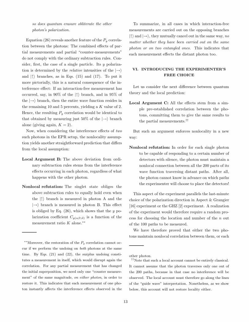
so does quantum erasure obliterate the other

photon’s polarization.

Equation (26) reveals another feature of the Py correla-

tion between the photons: The combined effects of par-

tial measurements and partial “counter-measurements”

do not comply with the ordinary subtraction rules. Con-

sider, first, the case of a single particle. Its y polariza-

tion is determined by the relative intensities of the |→〉and |↑〉 branches, as in Eqs. (15) and (17). To put it

more pictorially, this is a natural consequence of the in-

terference effect: If an interaction-free measurement has

occurred, say, in 90% of the |↑〉 branch, and in 95% of

the |→〉 branch, then the entire wave function resides in

the remaining 10 and 5 percents, yielding a K value of 2.

Hence, the resulting Py correlation would be identical to

that obtained by measuring just 50% of the |→〉 branch

alone (giving again, K = 2).

Now, when considering the interference effects of two

such photons in the EPR setup, the nonlocality assump-

tion yields another straightforward prediction that differs

from the local assumption:

Local Argument B: The above deviation from ordi-

nary subtraction rules stems from the interference

effects occurring in each photon, regardless of what

happens with the other photon.

Nonlocal refutation: The singlet state obliges the

above subtraction rules to equally hold even when

the |↑〉 branch is measured in photon A and the

|→〉 branch is measured in photon B. This effect

is obliged by Eq. (26), which shows that the y po-

larization coefficient Cy(αβγδ) is a function of the

measurement ratio K alone.∗∗

∗∗Moreover, the restoration of the Py correlation cannot oc-

cur if we perform the undoing on both photons at the same

time. By Eqs. (21) and (22), the surplus undoing consti-

tutes a measurement in itself, which would disrupt again the

correlation. For any partial measurement that has changed

the initial superposition, we need only one “counter measure-

ment” of the same magnitude, on either photon, in order to

restore it. This indicates that each measurement of one pho-

ton instantly affects the interference effects observed in the

To summarize, in all cases in which interaction-free

measurements are carried out on the opposing branches

|↑〉 and |→〉, they mutually cancel out in the same way, no

matter whether they have been carried out on the same

photon or on two entangled ones. This indicates that

each measurement effects the distant photon too.

VI. INTRODUCING THE EXPERIMENTER’S

FREE CHOICE

Let us consider the next difference between quantum

theory and the local prediction:

Local Argument C: All the effects stem from a sim-

ple pre-established correlation between the pho-

tons, committing them to give the same results to

the partial measurements.††

But such an argument enforces nonlocality in a new

way:

Nonlocal refutation: In order for each single photon

to be capable of responding to a certain number of

detectors with silence, the photon must maintain a

nonlocal connection between all the 200 parts of its

wave function traversing distant paths. After all,

the photon cannot know in advance on which paths

the experimenter will choose to place the detectors!

This aspect of the experiment parallels the last-minute

choice of the polarization direction in Aspect & Grangier

[16] experiment or the GHZ [2] experiment. A realization

of the experiment would therefore require a random pro-

cess for choosing the location and number of the n out

of the 100 paths to be measured.

We have therefore proved that either the two pho-

tons maintain nonlocal correlation between them, or each

other photon.††Note that such a local account cannot be entirely classical.

It cannot assume that the photon traverses only one out of

the 200 paths, because in that case no interference will be

observed. The local account must therefore go along the lines

of the “guide wave” interpretation. Nonetheless, as we show

below, this account will not restore locality either.

13

0.00%

10.00%

20.00%

30.00%

40.00%

50.00%

60.00%

0 2 4 6 8 10

ρρρρ

1-Cy

Disagreement A-C Disagreement A-B plus B-C

Chart 4. The disagreement between observers A and C is higher that the sum of disagreement between A and B plus B

and C for a broad range of ratios, disproving locality by breaking a Bell-like inequality.

photon maintains nonlocal correlation between its dis-

tant beams. The latter interpretation would join Hardy’s

[17,18] and Albert et al.’s [19] proofs for the nonlocality

of a single photon. Either way, nonlocality is inescapable.

The setup in Fig. 7 also points out the difficulty in ap-

plying counterfactuals to quantum mechanics: Suppose

we measure 50 of the 100 |↑〉 beams of photon A. A pos-

sible result of such an experiment might be that photon

A finishes in the |ր〉 path, while photon B goes on the

|ց〉 path.

A possible description of such a situation will be:

There is a 3% probability that the photons will be anti-

correlated, and this is one of those cases. But then, a

counterfactual can be presented: What would have been

the result had we placed detectors in front of 50 out of

the 100 beams of the |↑〉 branch of photon B too? The

answer is intriguing: Since doing so will completely undo

the measurement on photon A, photon B must either

hit one of the 50 detectors or completely agree with the

y measurement of photon A. Since our photon did not

agree with it, it must have been captured by one of the

50 detectors!

This imposes another odd counterfactual:

When we place a battery of counter-

measuring detectors on path B, they “magi-

cally” capture all the photons that were about

to disagree with the y measurement of photon

A, have we not placed the counter-measuring

detectors.

Such a teleological view is, of course, alien to physics.

One must rather accept the objective reality of the wave-

function. Only such a view can accept that the 50 de-

tectors on photon B cancel exactly the 50 measurements

done on photon A.

VII. AN INEQUALITY FOR PARTIAL

MEASUREMENTS

Let us now give a general nonlocality proof for partial

measurements. We shall consider a local hypothesis that

tries to maintain locality despite the above predictions

and show that it must violate an inequality theorem.

Local Argument D: Each pair of photons uses a pre-

14

established algorithm that assigns a definite Py

value for each partial measurement: For any num-

ber of paths that were interaction-freely measured,

the photons would yield some preestablished y po-

larization. The resulting list of Py values is infinite,

matching every possible degree of partial measure-

ment.

Nonlocal refutation: The alleged algorithm must sat-

isfy two restrictions: (1) In every pair, both pho-

tons must obey the same algorithm (though in re-

verse polarities): if photon A undergoes a measure-

ment of 30% on its |↑〉 branch, and photon B un-

dergoes the same measurement of its |→〉 branch,

their Py measurement must agree on each single

experiment (K = 1, hence Cy(αβγδ) = 1). This,

indeed, explains the apparent “erasure,” where op-

posite partial measurements on the two photons re-

store the initial correlations. (2) However, the al-

gorithm must assign the particular y polarization

to the ratio of the intensities of the photon’s |↑〉and |→〉 branches (that is α

β for photon A and γδ

for photon B). The correlation ratio Cy(αβγδ) makes

this fact evident: A measurement of 50% on the |↑〉branch of photon A yields α

β = 0.5, but many other

measurements on photon B will result γδ = 0.5 too

(0/50, 60/80, 80/90, etc.), equating Cy(αβγδ) to 1

and restoring the photons’ Py correlation.

Now, restrictions (1) and (2) refute the nonlocal

argument by breaking a Bell-like inequality in the

following way: Consider an experiment where pho-

ton A has αβ = 1.0 and photon B has γ

δ = 0.5. Here,

K = 0.5, hence Cy(αβγδ) = 0.97, implying that the

Py correlation between the photons is disrupted in

3% of the cases. If one believes in a pre-existing al-

gorithm directing each photon, the following coun-

terfactual must be true: Should B now had αβ = 0.5

and it repeated the same measurement, but with

a different opponent, C, with square the measure-

ment ratio: γδ = 0.25, the results must have been

the same! Since B must give a Py measurement

according to it’s αβ = 0.5 ratio, it must measure ex-

actly the same result that it gave for that ratio in

the actual experiment (in accordance with restric-

tion (1) – A and B must obey the same algorithm

– and restriction (2) – the algorithm depends onαβ alone). Since K remains with the same value

(1/0.5 = 0.5/0.25 = 2), Cy(αβγδ) remains 0.97, so

B and C must give non-correlated results in 3%

of the cases too. This imposes another counter-

factual: If A measured αβ = 1.0 against C with

γδ = 0.25, they could give, at most, different results

in 3% + 3% = 6% of the cases. However, when

we compute Cy(αβγδ) for this case (K = 4), the

result is 0.90. Which means that they must give

non-correlated results in 10% of the cases! Since

10% > 3% + 3%, that condition cannot be met,

and we conclude that the local argument is false.

Q.E.D.

This proof will be generalized below for a broad range

of ratios. That is, for a certain measurement ratio ρ, the

disagreement between A and C is greater than the sum of

disagreement between A and B plus B and C (see Chart

4):

If the difference between measurement ratios of parti-

cles A and B is K = ρ, the disagreement in Py measure-

ments will be:

∆A−B = 1 − Cy(αβγδ) = 1 −(

1 +√

ρ√2 + 2ρ

)2

. (31)

The difference between measurement ratios of B and C

will be ρ too, yielding the same value for ∆B−C (since

it depends on the ratio ρ alone), hence the maximal sum

of the disagreement between A and C will be twice the

above amount:

∆A−B + ∆B−C = 2 − 2

(

1 +√

ρ√2 + 2ρ

)2

. (32)

However, the measured disagreement between A and C

will be according to K = ρ2:

∆A−C = 1 −(

1 + ρ√

2 + 2ρ2

)2

. (33)

In Chart 4 we show the graphs of these functions,

which shows that in the region 1 < ρ < 8.3 the dis-

agreement ∆A−C is higher than the sum ∆A−B +∆B−C ,

thereby disproving any possible local explanation.

It should also be pointed out that Local Argument D

is especially ludicrous when we consider its post hoc ex-

planations for the unique quantitative features of joint

15

interferometry. Why should the ratio 50%-0% of mea-

surement and erasure give the same result as 75%-50%,

90%-80% and so on? A local model can “explain” these

phenomena only by adding arbitrary assumptions with-

out any rationale other than the need to account for such

unexpected results. In the nonlocal account, in contrast,

these peculiarities are straightforwardly derived from i)

the very nature of interference, and ii) the assumption

that the two interferometries affect one another due to

the quantum entanglement of the two photons.

Finally let the proof be extended to include all pairs:

Local Argument E: Perhaps only those photons that

give rise to partial measurements maintain nonlo-

cal correlation, while the others, which react to the

measurement with a click in the detectors (com-

plete measurement), have pre-fixed correlation and

do not affect one other nonlocally. These photons,

in other words, have “agreed” in advance to re-

spond to the detectors with clicks, and therefore

need not show correlation in their y polarization.

The refutation of this hypothesis (see also Ref. [20]) is

just like the proof we used in Section VI:

Nonlocal refutation: In order for some photons to be

capable of responding to a certain number of detec-

tors with a click, each such a photon must maintain

a nonlocal connection between the 200 distant parts

of its wave function. For the photon cannot know

in advance in which of the paths are detectors going

to be placed. Therefore, once the partial measure-

ments confirm the nonlocal prediction, the complete

measurements equally indicate nonlocal effects.

VIII. MULTIPLE PARTIAL MEASUREMENT

Since partial measurement does not take the cost of

disentanglement, it can be followed by many consecutive

partial measurements, all of which affect the distant en-

tangled particle. This is in marked contrast with the ordi-

nary EPR experiment, which allows the nonlocal transfer

of only one variable.

Consider the following case: Of two entangled parti-

cles, one undergoes partial measurement of its x polar-

ization, then of its y polarization, and then of its z po-

larization‡‡. Suppose also that all partial measurements

were very close to 100% (say, 90% each). Of course, such

a multitude of measurements increases the probability for

a click which would ruin the experiment, but if all partial

measurements succeeded, the state of the two entangled

particles is:

P⊙190% · Pր190% · P↑190%· |EPR〉. (34)

The resulting pair of particles is poorly correlated, but

an inverted set of counter measurements, performed on

the particle that was measured, can restore the initial

correlation. Since measurements in orthogonal directions

cannot commute, the counter measurements must be per-

formed in a reverse order:

P→190% · Pց190%

·(P⊗190% · P⊙190%)

·Pր190% · P↑190%· |EPR〉= P→190% · (Pց190% · Pր190%) · P↑190%· |EPR〉= (P→190% · P↑190%)· |EPR〉=|EPR〉. (35)

In general, any set of partial measurements gives a com-

plex linear combination of the kind:

|Ψ〉 = (a + ib) |↑〉1 |↑〉2 + (c + id) |→〉1 |→〉2+(e + if) |↑〉1 |→〉2 + (g + ih) |→〉1 |↑〉2. (36)

A pair of particles, therefore, can carry up to eight real

parameters. Such a combination of states, once success-

fully created on one particle, shows up in the distant par-

ticle too, a case that is impossible in the ordinary EPR

experiment. In terms of quantum information, this state

far exceeds the present, single-bit nonlocal correlation.

Let us note another interesting peculiarity of multi-

ple partial measurement: If one particle has undergone a

series of partial measurements, then the erasure of these

‡‡We will use the z ‘direction’ to denote a circular polar-

ization. The z direction is taken from the spin measurement

of spin-1/2 particles which obeys the same relations as the x,

y, and circular polarization measurement. The appropriate

operators will be P⊙α and P⊗α.

16

measurements can be attempted only in the reverse order

(last first, first last). If, however, the erasure is attempted

on the other particle of the entangled pair – even after a

time-like interval – the order of the erasures must be of

that of the measurements (first first, last last). This fact

seems to lend support to Cramer’s [21] “transactional in-

terpretation,” where the measurement of one particle af-

fects the other particle by traversing a “Feynman zigzag”

through time.

IX. THE NEW QUANTUM ERASURE AND ITS

SIGNIFICANCE

“Quantum erasure” denotes an operation that consti-

tutes the time reversal of the measurement process, undo-

ing the the measurement’s outcome and turning the wave

function back to its initial pure state. It has become the

focus of intensive study during the last few years because

of its far-reaching theoretical and technological bearings,

such as quantum computation and reversibility.

Most notable of these works is that of Scully et al., [22]

who demonstrated erasure of a quantum measurement in

a double-slit experiment with atoms. In this experiment,

the two parts of the wave function, prior to being re-

united, pass through a small cavity where they undergo

a measurement that can tell which path the atom has

traversed. Immediately after the measurement, while the

beams are still inside the cavities, the “which path” infor-

mation is totally erased. Scully et al. showed that after

leaving the cavity, the two beams gave rise to normal

interference, just as if no measurement took place.

This experiment, however, has two shortcomings that

obscure the uniqueness of quantum erasure. First, the

experiment makes it impossible to know the actual re-

sult of the measurement that has been later erased. This

impossibility is imposed by the very definition of the ex-

periment: If an experimenter observes the result of a

measurement, this observation itself becomes part of the

measurement, hence erasure requires completely erasing

that observer’s brain processes as well. Therefore, one

can only infer that detection and its erasure took place

on one of the two beams, but never know which beam

gave rise to the initial click. The same holds for the

proposals of Greenberger & YaSin, [23] Becker, [24] and

others, reviewed and refined by Kwiat et al. [25].

Our proposal overcomes this limitation. When the

measurement is partial, it is as observable as any other

measurement, and similarly its erasure. The reason for

this has been pointed out earlier: Unlike the prevail-

ing techniques, ours does not require time-reversing any

measuring instrument, thereby avoiding the enormous

technical difficulties involved with proper atomic control

and thermodynamic isolation. Rather, the only ther-

modynamic price we have to pay is that, the closer the

measurement gets to a complete measurement, the more

likely it is to end up in a click, whereby erasure will

be no more possible. Similarly, erasure itself might end

up in a click. We thus comply with the Second Law of

Thermodynamics at the statistical level. Still, in a large

enough series of experiments, we can have many cases

in which we can directly observe a measurement that is

close enough to complete measurement, and then observe

its complete erasure.

But the most intriguing consequence of quantum era-

sure is obscured by the second shortcoming of Scully et

al.’s experiment: They carried out the measurement and

its erasure on both halves of the wave function. This, we

suggest, is not only unnecessary but suppresses the non-

local aspect of the process. Elitzur [26] has proposed to

repeat Scully’s experiment dropping one of the measure-

ment and its erasure on one side. The argument was that

if interference shows up in this case too, it would prove

that undoing one half of the wave function instantly “un-

measures” the other half too. However, this proposal suf-

fers from the same shortcoming as the above erasure ex-

periments: The measurement and its erasure can only be

inferred and never directly observed. Brun and Barnett,

[27] on the other hand, proposed to carry out the mea-

surement on one arm and the cancellation on the other,

arguing that both operations should affect both arms.

Unfortunately, all these experiments study single-

particle interference, where the two parts of the wave

function are eventually reunited. This does not allow

nonlocality to be tested. A local theory could argue

that both the measurement and its erasure affect only

the measured half.

Partial measurement, again, overcomes all these short-

comings. It allows a direct observation of both the mea-

17

surement and its erasure. Furthermore, by performing

the measurement on one photon and the erasure on the

other, and by not uniting the two distant photons, we are

in a position to affirm: Not only quantum measurement,

but also its erasure, affects the other particle in the EPR

experiment. Notice also that, unlike the micromaser cav-

ities and laser beams in Scully et al.’s experiment, our

method carries out the erasure by much simpler optical

means.

X. CONCEPTUAL IMPLICATIONS

In a discussion that has become a classic, Feynman

[28] defined the double-slit experiment as “the core of the

mystery of quantum mechanics.” Albert [29] has gener-

alized this insight in his lucid exposition of quantum me-

chanics, where he showed that any quantum-mechanical

variable is a superposition of another, noncommuting

one. He went on to show how any variable could emerge

from the interference effect of its conjugate.

This is what the present work does with the x and y po-

larizations, illustrating the uncertainty principle by the

familiar phenomenon of interference. It is this highly vi-

sualizable phenomenon upon which the present proof for

nonlocality is based, not requiring Bell’s theorem. In so

doing, we have also extended the EPR argument to two

conclusions: i) Nonlocal effects are caused not only by a

complete measurement but even by its minutest stages.

ii) Nonlocal effects are caused not only by a measurement

but also by the time-reversed process. Therefore, nonlo-

cality needs not cease once the two particles in the EPR

experiment are measured; they can remain entangled in

spite of many successive measurements, maintaining the

strange “dialogue” between them for a long time.

Our proof also extends Bell’s proof in that, whereas

Bell’s inequality is based on the polarization measure-

ments along varying angles, we present a new inequality

that holds within the same angle of polarization for both

particles.

Partial measurement gives a new twist to the question

whether God plays dice. Our experiment shows that not

only does God cast a dice every time a polarization mea-

surement is performed, but that, when the dice takes

some time to fall, God preserves the right to change His

mind as many times as He pleases. He can, for example,

give 99% for a particle to have a |↑〉 polarization, and

then, upon the 100th partial measurement, change His

mind and make the polarization |→〉. Give Him further

opportunities by dividing the 100th measurement into

further 100 partial measurements, and He might change

his mind time and again. §§

To summarize, our proof highlights a fundamental pe-

culiarity of quantum mechanics. Suppose that a classical

object resides in one out of 200 closed boxes. Opening

some boxes and not finding the object there only alters

the observer’s knowledge (or, better, ignorance) about the

object’s location. In quantum mechanics, in contrast, ev-

ery such non-detection brings about a real change in the

particle’s state, empirically proved in our EPR-PM set-

ting with utmost quantitative precision. It is this lack of

differentiation between ontology and epistemology – any

change in the observer’s knowledge corresponding to pre-

cisely the same change in the state of the thing observed

– that makes quantum mechanics so unique among all

natural sciences.

ACKNOWLEDGMENTS

An early version of this work was presented at the Gor-

don Conference on Modern Developments in Thermody-

namics, Ventura, USA, February 1997. Thanks are due

to the participants for their helpful comments. It is also

a pleasure to thank Yakir Aharonov, Daniel Rohrlich and

Lev Vaidman for illuminating discussions.

[1] J. S. Bell, Physics, 1, 195 (1964).

[2] D. M. Greenberger, M. A. Horne, and A. Zeilinger, Bell’s

Theorem, Quantum Theory, and Conceptions of the Uni-

§§This bearing of partial measurement on the issue of deter-

minism vs. indeterminism makes it also relevant to the origins

of time-asymmetry, see [30–32].

18

verse, edited by M. Kafatos, pp. 73-76. (Kluwer Aca-

demic, Dordrecht, 1989).

[3] L. Hardy, Phys. Rev. Lett. 71, 1665 (1993).

[4] A. C. Elitzur, and L. Vaidman, Found. Phys. 23, 987

(1993).

[5] L. Hardy, Phys. Rev. Lett. 68, 2981 (1992).

[6] P. Kwiat, H. Weinfurter, T. Herzog, A. Zeilinger, and M.

A. Kasevich, Phys. Rev. Lett. 74, 4763 (1995).

[7] R. Penrose, Shadows of the Mind (Oxford University

Press, Oxford, 1994).

[8] L. Vaidman, Are interaction-free measurements interac-

tion free? International Conference on Quantum Optics,

Raubichi, Belarus (2000). quant-ph/0006077.

[9] W. K. Wooters and W. H. Zurek, Phys. Rev. D 19, 473

(1979).

[10] S. Dorr, T. Nonn, and G. Rempe, Phys. Rev. Lett. 81,

5705 (1998).

[11] H. R. Brown, J. Summhammer, R. E. Callaghan, and P.

Kaloyerou, Phys. Lett. A 163, 21 (1992).

[12] P. N. Kaloyerou and H. R. Brown, Physica A 176, 78

(1992).

[13] L. C. Ryff, Phys. Lett. A 170, 259 (1992).

[14] L. C. Ryff, Mysteries, Puzzles, and Paradoxes in

Quantum Mechanics (AIP Conference Proceedings 461),

edited by R. Bonifacio, pp. 251-254. (American Institute

of Physics, Woodbury, NY, 1999).

[15] D. Deutsch, A. Ekert, R. Jozsa, C. Macchiavello, S.

Popescu, and A. Sanpera, Phys. Rev. Lett. 77, 2818

(1996).

[16] A. Aspect and P. Grangier, Quantum Concepts in Space

and Time, edited by R. Penrose and C. J. Isham (Oxford

University Press, Oxford, 1986).

[17] L. Hardy, Phys. Rev. Lett. 73, 2279 (1994).

[18] L. Hardy, Phys. Rev. Lett. 68, 2981 (1992).

[19] D. Albert, Y. Aharonov, and S. D’Amato, Phys. Rev.

Lett. 54, 5 (1985).

[20] A. C. Elitzur, S. Popescu, and D. Rohrlich, Phys. Lett.

A 162, 25 (1992).

[21] J. G. Cramer, Rev. Mod. Phys., 58, 647 (1986).

[22] M. O. Scully, B. G. Englert, and H. Walther, Nature,

351, 111 (1991).

[23] D. Greenberger and A. YaSin, Found. Phys. 19, 679

(1989).

[24] L. Becker, Phys. Lett. A249, 19 (1998).

[25] P. G. Kwiat, A. M. Steinberg, and R. Chiao, Phys. Rev.

A 49, 61 (1994).

[26] A. C. Elitzur, Astrophys. and Space Sci. 244, 313 (1996).

[27] T. A. Brun and S. M. Barnett, J. Modern Optics. 45,

777 (1998).

[28] R. P. Feynman, R. B. Leighton, and M. Sands, The Feyn-

man Lectures (Addison-Wesley, New York, 1965).

[29] D. Z. Albert, Quantum Mechanics and Experience (Har-

vard University Press, Cambridge, MA., 1996).

[30] A. C. Elitzur and S. Dolev, Phys. Lett. A 251, 89 (1999).

Erratum, A255, 369, (1999), gr-qc/0012060.

[31] A. C. Elitzur and S. Dolev, Found. Phys. Lett. 12,

309(1999), quant-ph/0012081.

[32] A. C. Elitzur and S. Dolev, Phys. Lett. A 266, 268

(2000), gr-qc/0012061.

19