Eur. Phys. J. Plus (2021) 136:847 https://doi.org/10.1140/epjp/s13360-021-01835-9

Regular Art icle

Can classical electrodynamics predict nonlocal effects?

José A. Heras1 , Ricardo Heras2,a

1 Instituto de Geofísica, Universidad Nacional Autónoma de México, Ciudad de México 04510, México2 Department of Physics and Astronomy, University College London, London WC1E 6BT, UK

Received: 7 May 2021 / Accepted: 3 August 2021© The Author(s) 2021

Abstract Classical electrodynamics is a local theory describing local interactions betweencharges and electromagnetic fields and therefore one would not expect that this theory couldpredict nonlocal effects. But this perception implicitly assumes that the electromagneticconfigurations lie in simply connected regions. In this paper, we consider an electromagneticconfiguration lying in a non-simply connected region, which consists of a charged particleencircling an infinitely long solenoid enclosing a uniform magnetic flux, and show that theelectromagnetic angular momentum of this configuration describes a nonlocal interactionbetween the encircling charge outside the solenoid and the magnetic flux confined inside thesolenoid. We argue that the nonlocality of this interaction is of topological nature by showingthat the electromagnetic angular momentum of the configuration is proportional to a windingnumber. The magnitude of this electromagnetic angular momentum may be interpreted asthe classical counterpart of the Aharonov–Bohm phase.

1 Introduction

Three years after the publication of the seminal paper by Aharonov and Bohm [1] on theprediction of the effect that now bears their name, the Aharonov–Bohm (AB) effect, Tassie andPeshkin [2] claimed that “... the quantum mechanical effects of the inaccessible field can beunderstood, both mathematically and physically, through angular momentum considerations...” They argued that in regions where electrons encircling inaccessible magnetic fields,classical physics predicts that, in addition to the mechanical angular momentum: Lm =(r×mv)z , there is an electromagnetic angular momentum along the z-axis whose magnitudeis given by

Lz = eΦ

2πc, (1)

where e is the electron charge and Φ is the inaccessible magnetic flux. The interesting pointis that in these same free-field regions, quantum mechanics predicted the existence of the ABphase δ = eΦ/(hc). However, the comments of Tassie and Peshkin received little attentionand the idea that (1) could shed light on the interpretation of the AB effect did not seemto have been explored further until in recent years in which Tiwari [3] and Wakamatsu etal. [4] derived (1) and drew attention to the role that plays (1) in the context of the AB

a e-mail: ricardo.heras.13@ucl.ac.uk (corresponding author)

0123456789().: V,-vol 123

847 Page 2 of 19 Eur. Phys. J. Plus (2021) 136:847

effect. In this paper, we examine in detail the configuration formed by a charged particleencircling an infinitely long solenoid enclosing a uniform magnetic flux and show that thisparticle moves in a non-simply connected region where there is no magnetic field but there isa nonzero vector potential. We then show that (1) is the electromagnetic angular momentumof this configuration. In contrast to Tiwari [3] and Wakamatsu et al. [4], who discuss (1) inconnection to the AB effect, we only consider this connection when we suggest that (1) maybe interpreted as the classical counterpart of the AB phase. Our main purpose here is to arguethat (1) describes a nonlocal interaction between the charge moving outside the solenoid andthe magnetic flux inside this solenoid, which answers in the affirmative the question posedin the title of this paper. Throughout our study we emphasise the topological and nonlocalfeatures of (1).

2 Charge-solenoid configuration

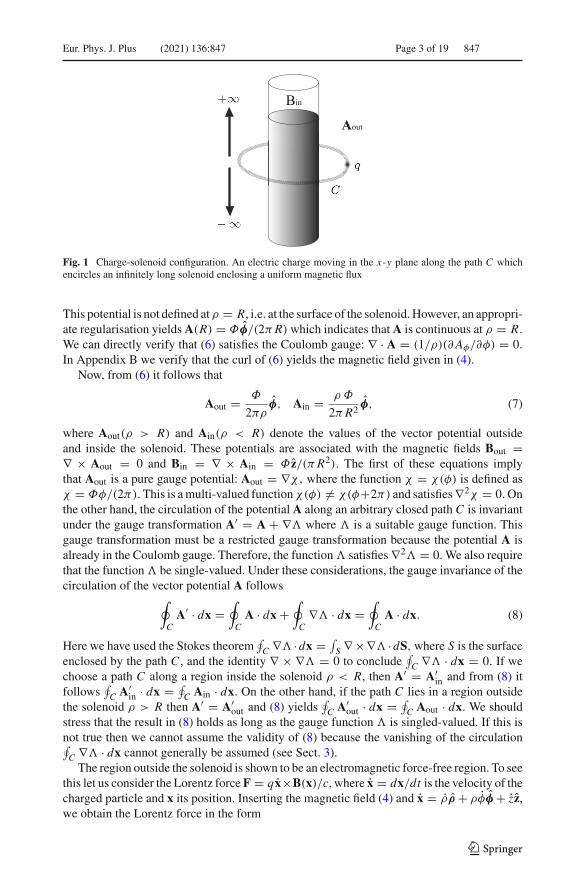
Consider the charge-solenoid configuration, which consists of a particle having the charge qand mass m and continuously moving around an infinitely long solenoid of radius R whichencloses a uniform magnetic flux Φ. The z-axis is chosen as the axis of the solenoid (SeeFig. 1). We use Gaussian units and cylindrical coordinates (ρ, θ, φ) with their correspondingunit vectors (ρ,θ ,φ). The electric current density of the infinitely long solenoid is given by

J = cΦδ(ρ − R)

4π2R2 φ, (2)

where δ(ρ − R) is the Dirac delta function and Φ = πR2B is the magnetic flux through thesolenoid with B being the magnitude of the uniform magnetic field inside the solenoid. Theelectric current density J is a steady current: ∇ · J = 0 and its magnetic field satisfies themagnetostatic equations

∇ · B = 0, ∇ × B = Φδ(ρ − R)

πR2 φ, (3)

whose solution gives the explicit form of this magnetic field

B = ΦΘ(R − ρ)

πR2 z, (4)

which is confined in the solenoid. Here Θ(ρ − R) is the Heaviside step function having thevalues Θ = 1 if R > ρ and Θ = 0 if R < ρ. To verify that (4) satisfies (3) we writeB = Bz(ρ)z, where Bz(ρ) = ΦΘ(R −ρ)/(πR2). Thus, ∇ · B = ∂Bz/∂z = 0 and ∇ × B =−(∂Bz/∂ρ)φ = Φδ(ρ − R)φ/(πR2), where we have used ∂Θ(R − ρ)/∂ρ = −δ(ρ − R).From (4) it follows that Bout = 0 and Bin = Φ z/(πR2), where Bout(ρ > R) and Bin(ρ < R)

denote the values of the magnetic field outside and inside the solenoid. The magnetic fieldvanishes outside the solenoid and has a constant value inside it. From the first equation in(3) we infer B = ∇ × A where A is the corresponding vector potential. Using this relationin the second equation in (3), considering ∇2F = ∇(∇ · F) − ∇ × (∇ × F) and adopting theCoulomb gauge ∇ · A = 0, we obtain the Poisson equation

∇2A = −Φδ(ρ − R)

πR2 φ. (5)

In Appendix A we verify that the solution of this equation reads [5]:

A = Φ

2π

(Θ(ρ − R)

ρ+ ρ Θ(R − ρ)

R2

)φ. (6)

123

Eur. Phys. J. Plus (2021) 136:847 Page 3 of 19 847

Fig. 1 Charge-solenoid configuration. An electric charge moving in the x-y plane along the path C whichencircles an infinitely long solenoid enclosing a uniform magnetic flux

This potential is not defined at ρ = R, i.e. at the surface of the solenoid. However, an appropri-ate regularisation yields A(R) = Φφ/(2πR) which indicates that A is continuous at ρ = R.

We can directly verify that (6) satisfies the Coulomb gauge: ∇ · A = (1/ρ)(∂Aφ/∂φ) = 0.

In Appendix B we verify that the curl of (6) yields the magnetic field given in (4).Now, from (6) it follows that

Aout = Φ

2πρφ, Ain = ρ Φ

2πR2 φ, (7)

where Aout(ρ > R) and Ain(ρ < R) denote the values of the vector potential outsideand inside the solenoid. These potentials are associated with the magnetic fields Bout =∇ × Aout = 0 and Bin = ∇ × Ain = Φ z/(πR2). The first of these equations implythat Aout is a pure gauge potential: Aout = ∇χ, where the function χ = χ(φ) is defined asχ = Φφ/(2π). This is a multi-valued function χ(φ) �= χ(φ+2π) and satisfies ∇2χ = 0. Onthe other hand, the circulation of the potential A along an arbitrary closed path C is invariantunder the gauge transformation A′ = A + ∇� where � is a suitable gauge function. Thisgauge transformation must be a restricted gauge transformation because the potential A isalready in the Coulomb gauge. Therefore, the function � satisfies ∇2� = 0. We also requirethat the function � be single-valued. Under these considerations, the gauge invariance of thecirculation of the vector potential A follows∮

CA′ · dx =

∮C

A · dx +∮C

∇� · dx =∮C

A · dx. (8)

Here we have used the Stokes theorem∮C ∇� ·dx = ∫

S ∇ ×∇� ·dS, where S is the surfaceenclosed by the path C , and the identity ∇ × ∇� = 0 to conclude

∮C ∇� · dx = 0. If we

choose a path C along a region inside the solenoid ρ < R, then A′ = A′in and from (8) it

follows∮C A′

in · dx = ∮C Ain · dx. On the other hand, if the path C lies in a region outside

the solenoid ρ > R then A′ = A′out and (8) yields

∮C A′

out · dx = ∮C Aout · dx. We should

stress that the result in (8) holds as long as the gauge function � is singled-valued. If this isnot true then we cannot assume the validity of (8) because the vanishing of the circulation∮C ∇� · dx cannot generally be assumed (see Sect. 3).

The region outside the solenoid is shown to be an electromagnetic force-free region. To seethis let us consider the Lorentz force F = q x×B(x)/c, where x = dx/dt is the velocity of thecharged particle and x its position. Inserting the magnetic field (4) and x = ρρ + ρφφ + zz,we obtain the Lorentz force in the form

123

847 Page 4 of 19 Eur. Phys. J. Plus (2021) 136:847

F = qΦΘ(R − ρ)

πR2 (ρφρ − ρφ), (9)

which is local in the sense that the magnetic field must be evaluated at the point wherethe particle is located. It follows that if the particle is located inside the solenoid ρ < Rthen Θ = 1 and we obtain F = qΦ(ρφρ − ρφ)/(πR2). However, in the charge-solenoidconfiguration the moving charged particle is assumed to be outside the solenoid ρ > R sothat Θ = 0 and therefore F = 0. In short: the Lorentz force vanishes because the magneticfield is zero in the region where the charge is moving.

3 Topology and nonlocality of the circulation of the vector potential outside thesolenoid

The Cauchy’s integral formula [6] for an analytic function f (z) reads,

1

2π i

∮C

f (z) dz

z−z0=

{n(C, z0) f (z0) if C encloses z0

0 otherwise(10)

where n(C, z0) represents the winding number of the curve C around the singularity z0. Thewinding number gives the number of times the curve C encircles (counterclockwise) arounda singularity. Consider now the particular case in which there is a singularity at ρ = 0, whichin the complex plane corresponds to z0 = ρ eiφ = 0. We choose f (z) = K , where K is aconstant and thus (10) yields

K

2π i

∮C

dz

z=

{nK if C encloses z0 = 00 otherwise

(11)

If we write z = ρ eiφ and dz = eiφ(dρ + iρdφ) then it follows that dz/z = (1/ρ)dρ +idφ. Therefore, the left-hand side of (11) gives rise to two terms. The first term reads(K/2π i)

∮C dρ/ρ but dρ/ρ = (ρ/ρ) · dx = ∇ ln (ρ) · dx, where dx = dρρ + ρdφφ + dzz

is the line element, implying∮C ∇ ln (ρ) · dx = 0 because ln (ρ) is a single-valued func-

tion and consequently this first term vanishes. The second term is non-vanishing and reads(K/2π)

∮C dφ. Since dφ = φ/ρ · dx then (11) takes the particular form

∮C

(K φ

2πρ

)· dx =

{nK if C encloses ρ = 00 otherwise

(12)

This is a purely formal result arising from the Cauchy’s integral formula given in (10). Letus now apply (12) to an idealised infinitely long solenoid enclosing a uniform magneticflux Φ. We make the identification K = Φ in (12) and obtain the relation K φ/(2πρ) =Φφ/(2πρ) = Aout(x). Since the solenoid encloses the singularity at ρ = 0 then it follows∮

CAout ·dx =

{nΦ if C encloses the solenoid0 otherwise

(13)

Here n denotes the winding number of the curve C around the solenoid. Equation (13) statesthat if the curve C encircles n times the solenoid then the circulation of the potential Aout

accumulates n times the magnetic flux Φ. The circulation of the vector potential in (13) isconstant since nΦ is a constant quantity and therefore this circulation is insensitive to theform of the curve C and also to the dynamics that we can associate to this curve. If forexample we consider C1,C2...Ck different curves which enclose counterclockwise n timesthe solenoid then (13) implies the equalities

123

Eur. Phys. J. Plus (2021) 136:847 Page 5 of 19 847

Fig. 2 a The circulation of the potential Aout in a closed path around the solenoid is insensitive to the formof the path, i.e. for different paths C1,C2...Ck with the same winding number we have

∮C1

Aout(x) · dx =∮C2

Aout(x) ·dx = ... = ∮Ck

Aout(x) · dx. b The circulation∮C>∂S Aout · dx is taken along a path C greater

than the boundary ∂S of the surface S of the solenoid. Since∮C>∂S Aout · dx = ∫

S Bin · dS holds then thecirculation is spatially delocalised from the surface of the solenoid where the flux of the magnetic field islocalised

∮C1

Aout · dx =∮C2

Aout ·dx = ... =∮Ck

Aout · dx. (14)

The curves C1,C2...Ck are homotopically equivalent (one curve can be continuouslydeformed into the other) and therefore we could not distinguish if the flux Φ in (13) isconnected with the circulation of Aout along C1 or along C2 or along Ck (see Fig. 2a). Thisindistinguishability is a manifestation of the topology of the infinitely long solenoid whichlies in a non-simply connected region.

Let us discuss the nonlocal feature of the circulation of the potential Aout. At first sight,we could naively transform the closed line integral that defines this circulation into a surfaceintegral via the Stokes theorem:

∮C=∂S Aout ·dx = ∫

S ∇ ×Aout ·dS, where the closed pathC now represents the boundary ∂S of some suitable surface S . However, this application ofthe Stokes theorem leads to an inconsistent result because the potential Aout is the gradientof a function and therefore ∇ × Aout = 0, which implies the vanishing of the circulation ofAout, a result that contradicts (13) because it is assumed that the pathC encloses the solenoid.However, we can consistently use the Stokes theorem but we need to be careful in applyingit by taking into account that the path C encloses ρ = 0 and thus the considered region isnon-simply connected and therefore

∮C A · dx �= 0.

Consider the vector potential A in (6) which is defined in all space. Let us apply theStokes theorem to this potential:

∮C=∂S A · dx = ∫

S ∇ × A · dS. If the path C encloses thesolenoid then along this path the potential in (6) reads A = Aout and the Stokes theorem gives:∮C=∂S Aout · dx = ∫

S ∇ × A · dS. In this case the surface S enclosed by the path C can bewritten asS = S0+S, where S0 is the surface extending outside the solenoid to the boundary∂S and S is the surface accounting for the cross section of the solenoid and having theboundary ∂S (see Fig. 2b). We observe that the boundary of the surface of the solenoid satisfiesC=∂S >∂S because the path C is outside the solenoid (C > ∂S indicates that the length ofthe curve C is greater than the length of the boundary ∂S of the solenoid). Along the surfaceS0 the potential in (6) reads A = Aout and along the solenoid surface S it becomes A = Ain.

Thus, the Stokes theorem gives:∮C=∂S Aout · dx = ∫

S0∇ × Aout · dS + ∫

S ∇ × Ain · dS.

The first term on the right vanishes because ∇ × Aout = 0 and thus the Stokes theorem takesthe form

123

847 Page 6 of 19 Eur. Phys. J. Plus (2021) 136:847

∮C>∂S

Aout · dx =∫S∇ × Ain · dS, (15)

which admits a nonlocal interpretation. While the left-hand side of (15) is defined outside thesolenoid, its right-hand side is defined inside the solenoid. Put differently, the sides of (15)are defined in different spatial regions which implies a nonlocal connection between them.We can see that this nonlocality is a consequence of having applied the Stokes theorem in anon-simply connected region (we observe that

∮C Aout ·dx = ∮

C ∇χ ·dx �= 0) and ultimatelyis a consequence of the topology of the idealised solenoid. The genesis of this topology liesin the fact that in the assumption of an infinitely long solenoid there is a non-removablesingularity along the z-axis. Since ∇ × Ain = Bin, with Bin denoting the constant magneticfield inside the solenoid, then (15) becomes

∮C>∂S

Aout · dx =∫S

Bin · dS, (16)

which expresses a nonlocal relation between the magnetic flux confined in the solenoid andthe circulation of the vector potential along a curve outside the solenoid. Equations (14) and(16) imply

∮Ck>∂S

Aout · dx = ... =∮C2>∂S

Aout · dx =∮C1>∂S

Aout · dx =∫S

Bin · dS, (17)

Now, if we consider the equalities of the left-hand side of the magnetic flux in Eq. (17) thenthere is a manifest ambiguity because we cannot distinguish if this flux is connected withthe circulation of Aout along C1 > ∂S or along C2 > ∂S or along Ck > ∂S. This meansthat the circulations in (17) are spatially delocalised with respect to the magnetic flux, anexpected result since they are not functions of point. Put in other words: the potential Aout isambiguous due to its gauge-dependence and its circulation

∮C Aout ·dx is ambiguous due to its

spatial delocalisation (indistinguishability of the curveC). We should also note the differencebetween applying the Stokes theorem in a simply connected region and in the non-simplyconnected region considered here. In the former application of the theorem there is a singlecurve C = ∂S representing the boundary ∂S of the surface S. In the latter application ofthe theorem there can be k curves Ck > ∂S all of them greater than the boundary ∂S of thesurface S.

We can now draw the lessons we have learned about the infinitely long solenoid. Thecurrent of this solenoid (2) yields the vector potential A in (6) whose part outside the solenoidis Aout and the magnetic field B in (4) whose part inside the solenoid is Bin. This infinitelylong solenoid involves a line of singularity (along the z-axis) and then one can apply theCauchy’s integral formula (10) and the Stokes theorem (16) to this non-simply connectedregion. Both mathematical tools lead to (17), which unambiguously shows the nonlocality ofthe circulation of Aout with respect to the flux of the magnetic field Bin. Physics deals with theinfinitely long solenoid and topology with the line of singularity and the homotopic curvesaround this line. One then can say that the idea of an infinitely long solenoid is the genesisof the nonlocality of the circulation of Aout, or alternatively, that the idea of an infinite lineof singularity is the genesis of this nonlocality. In more elegantly words: topology dictatesnonlocality! However, an infinitely long solenoid and a line of singularity are abstract ideasand therefore the moral of this story is that it all started by making idealisations.

123

Eur. Phys. J. Plus (2021) 136:847 Page 7 of 19 847

4 Electromagnetic angular momentum

Using the Poynting formula LP = [1/(4πc)] ∫V x × (E × B) d3x for an electromagneticangular momentum in a volume V , we come directly to the conclusion that the electromag-netic angular momentum of the charge-solenoid configuration vanishes outside the solenoidbecause the magnetic field is zero in this region. However, Wakamatsu et al. [4] recentlyused the Maxwell formula [7]: LM = (1/c)

∫V � x × A d3x for an electromagnetic angular

momentum and arrived at the conclusion that the electromagnetic angular momentum ofthe charge-solenoid configuration is given by L = qΦ z/(2πc) outside the solenoid. Thissame result was previously obtained by Tiwari [3] using a Lagrangian treatment. Why dothe Poynting and Maxwell formulas predict different results for the same configuration? Toanswer this question, let us formulate the following theorem:Decomposition Theorem. Let E(x, t) be a time-dependent electric field and �(x, t) = ∇ ·E/(4π) its associated charge density. Let B(x) be a time-independent magnetic field andA(x) its associated vector potential. The fields E and B are independent fields, i.e. theyare produced by different sources. The Poynting formula for the electromagnetic angularmomentum in the volume V originated by the interaction between the fields E and B is givenby

LP = 1

4πc

∫V

x × (E × B) d3x, (18)

and can be decomposed as

LP = LM + LR + LG + LS, (19)

where

LM = 1

c

∫V

� x × A d3x, (20)

LR = 1

4πc

∫V

x × [(∇ × E) × A

]d3x, (21)

LG = 1

4πc

∫V

x × (E∇ · A) d3x, (22)

LS = 1

4πc

∮S

x × [n(E · A) − A(n · E) − E(n · A)

]dS. (23)

Here S is the surface of the volume V . The proof of this theorem is given in two parts. InAppendix C we show that the validity of (18) follows from the Poynting vector associatedwith the interacting fields E and B, and in Appendix D we show that (19) follows from atensor identity.

The term LR in (21) contains the factor ∇ ×E which is connected with (−1/c)∂B/∂t dueto the Faraday’s induction law and therefore it deals with possible radiative effects. The termLG in (22) involving ∇ · A deals with the adopted gauge for the potential A. The term LS in(23) is a surface term. Notice that LP may be zero without LM necessarily be zero, whichexplains why the Poynting and Maxwell formulas can predict different results as it happenswhen considering the charge-solenoid configuration.

Let us now apply (19) to this charge-solenoid configuration where the volume V coversall space except the volume of the solenoid. Here we have LP = 0 because B = 0 outsidethe solenoid and therefore (19) yields 0 = LM + LR + LG + LS. In Appendix E we showthat LR = 0. We have also LG = 0 because ∇ · Aout = 0. The surviving pieces satisfy

123

847 Page 8 of 19 Eur. Phys. J. Plus (2021) 136:847

0 = LM + LS indicating that there exists LM in the volumetric space where the charge ismoving around the solenoid and there exists LS on the surface of this volumetric space whichlies at infinity. It follows that LS = −LM and this provides an interpretation for LS. We willsee that LM is related to the flux of the magnetic field of the solenoid and therefore LS maybe interpreted as an electromagnetic angular momentum originated by the return flux of themagnetic field of an infinitely long solenoid, an interpretation consistent with the fact thatthe signs of LM and LS are reversed. When considering the relation LM = −LS we shouldalways have in mind that LM and LS are defined in different spatial regions.

We also note that a different and less general two-dimensional decomposition of thePoynting formula LP was introduced by Wakamatsu et al. [4] (this decomposition containsa sign mistake), which involves a two-dimensional Coulomb field produced by the movingelectron whose velocity is assumed to be “much slower than the speed of light,” a condi-tion that, according to the authors, allows them to discard the magnetic field of the movingelectron. They obtained the relation LM = −LS and interpreted the piece −LS as an elec-tromagnetic angular momentum originated by the return flux. However, their analysis isunsatisfactory because the electron-solenoid configuration is three-dimensional, and moreimportantly, because they completely ignored the radiative effects of the moving electron.Even for slowly moving electrons with v << c there are radiation fields as we will show itin Appendix E, where we will explicitly demonstrate the non-trivial result that the electro-magnetic angular momentum of the charge-solenoid configuration is insensitive to radiativeeffects.

We now apply (20) to obtain the electromagnetic angular momentum of the charge-solenoid configuration covering all space except the surface S which lies at infinity.We assume that the charge q is localised in the x-y plane so that its position vectoris xq(t) = {ρq(t) cos φq(t), ρq(t) sin φq(t), 0} = ρq(t)ρ and �(x′, t) = (q/ρ′)δ{ρ′ −ρq(t)}δ{φ′ − φq(t)}δ{z′} is its associated charge density. The vector potential is given byAout(x′) = Φφ/(2πρ′). A generic point reads x′ = ρ′ρ+z′z. Using these ingredients andintegrating the right-hand side of (20), we obtain

1

c

∫V

�(x′, t) x′ × Aout(x′) d3x ′ = nqΦ

2πcz, (24)

where n is the winding number identifying the number of times the electric charge trav-els its closed path around the solenoid. In getting (24) we have used

∫ ∞−∞ δ(z′)dz′ =

1,∫ ∞−∞ z′δ(z′)dz′ = 0,

∫ ∞

Rδ{ρ′ − ρq(t)} dρ′ = Θ{ρq(t) − R} = 1, (25)

(because ρq(t) > R outside the solenoid) and the relation∮C

δ{φ′ − φq(t)} dφ′ = n, (26)

which is demonstrated in Appendix F. Therefore, (24) represents the accumulated electro-magnetic angular momentum of the charge-solenoid configuration

L = nqΦ

2πcz. (27)

Expressed differently, every time the charge goes around the solenoid, the charge-solenoidconfiguration acquires the electromagnetic angular momentum L(n=1) = qΦ z/(2πc) and

123

Eur. Phys. J. Plus (2021) 136:847 Page 9 of 19 847

therefore after n times this configuration accumulates the electromagnetic angular momen-tum given by (27), which can compactly be written as L = nL(n=1) (this equation doesnot represent a quantisation rule because L(n=1) does not generally describe a quantum ofelectromagnetic angular momentum).

Some additional comments on (27) are in order. The fact that this equation does notinvolve the coordinates of the encircling electric charge means that L is independent fromthe dynamics of this charge and therefore from its emitted radiation. This conclusion followsfrom the use of relations (25) and (26) in the computation of (24). It is clear that the useof these integrals embodies a loss of information of the dynamical coordinates ρq(t) andφq(t) of the encircling charge. Notice also that the corresponding electromagnetic angularmomentum LS lying on the infinite surface and associated with the return flux, is given byLS = −nqΦ z/(2πc) and therefore we have the relation LM + LS = 0 as predicted by thePoynting formula outside the solenoid. Here we justify the validity of this last relation byshowing that LP = LM + LR + LG + LS with LP = 0, LR = 0 and LG = 0. On the otherhand, when considering the Maxwell formula for the electromagnetic angular momentumapplied to the charge-solenoid configuration

L = 1

c

∫V

� x × Aout d3x, (28)

the question about its gauge invariance immediately arises. It is clear that this invariancerequires

∫V � x × ∇� d3x = 0 where � is a suitable gauge function. This condition is valid

for the charge-solenoid configuration. Let us express (28) in a form that makes evident itsgauge invariance. We have seen that the relation

∮C Aout · dx = nΦ given in (13) holds for

the potential outside the infinite solenoid where n is the winding number of the path C . Thisrelation and (27) yield the novel form

L = q z2πc

∮C

Aout · dx, (29)

which is gauge invariant on account of the gauge invariance of the circulation of the potentialAout. According to (29) the accumulated electromagnetic angular momentum depends onthe circulation of the potential outside the solenoid. Using (16) we can see that (29) can beexpressed as

L = q z2πc

∫S

Bin · dS, (30)

which states that the accumulated electromagnetic angular momentum calculated in a volumeV outside the solenoid depends on the flux of the magnetic field inside the solenoid. Atfirst glance, (29) and (30) suggest different interpretations of the physical origin of theelectromagnetic angular momentum L. Let us combine (29) and (30) to obtain the relation

q z2πc

∮C

Aout · dx = L = q z2πc

∫S

Bin · dS. (31)

The first interpretation, which we will call the A-explanation, is supported by the first equalityin (31), according to which the vector potential locally acts through its circulation on thecharged particle originating the electromagnetic angular momentum L. Argued differently,classical electrodynamics predicts the existence of an effect in the region outside the solenoid,the electromagnetic angular momentum L, which is physically originated by the local actionof an electromagnetic quantity on the charged particle. Now the only electromagnetic quantityfunction of point defined in that region is the potential Aout and therefore this potential should

123

847 Page 10 of 19 Eur. Phys. J. Plus (2021) 136:847

produce L. In short: Aout exists in each point of the trajectory of q and therefore Aout locallyacts on q producing L. The second interpretation, which we will call the B-explanation, issupported by the second equality in (31), according to which the magnetic field nonlocally actsthrough its flux on the charged particle originating the electromagnetic angular momentumL. In short: Bin exists inside the solenoid and not in each point of the trajectory of q outsidethe solenoid and therefore Bin nonlocally acts on q producing L. We admit the B-explanationand reject the A-explanation for the following arguments:(a) The potential Aout is gauge-dependent.(b) The Stokes theorem applied in a non-simply connected region implies the relation (see(17))

q z2πc

∮Ck>∂S

Aout · dx = ... = q z2πc

∮C2>∂S

Aout · dx = q z2πc

∮C1>∂S

Aout · dx = L = q z2πc

∫S

Bin · dS,

(32)

where the different charge paths C1 > ∂S,C2 > ∂S, ...,Ck > ∂S possessing all of them thesame winding number are homotopically equivalent. Now, if we consider the equalities of theleft-hand side of L in (32) then there is a manifest ambiguity because we cannot distinguishif L is connected with the circulation of Aout along C1 > ∂S or along C2 > ∂S or alongCk > ∂S. We cannot know which of the circulations of the potential Aout displayed in (32) iscausally connected with L because these circulations are spatially delocalised with respectto the solenoid (they are not functions of point). As pointed in Sect. 3, the potential Aout isambiguous due to its gauge-dependence and its circulation

∮C Aout ·dx is ambiguous due to its

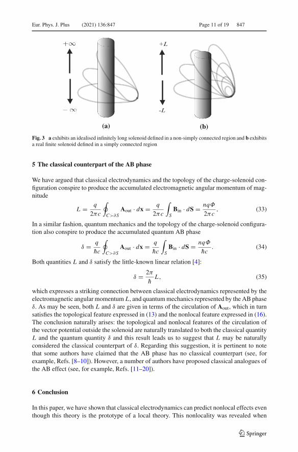
spatial delocalisation (indistinguishability of the curve C). Accordingly, the A-explanationdoes not hold. But if we consider the last equality in (32) then we conclude that L outsidethe solenoid is unambiguously connected with the flux of the magnetic field confined insidethe solenoid. Since the charge and the magnetic flux lie in different spatial regions then theynonlocally interact to produce L. Stated differently, (32) tell us that the magnetic flux doesnot locally affect the trajectory of the charge. We can now answer the question posed in thetitle of this paper: Can classical electrodynamics predict non-local effects? Answer: yes, theelectromagnetic relation given in (27) describes a nonlocal interaction between the magneticflux confined inside the solenoid and the electric charge moving outside the solenoid. Thiselectromagnetic configuration lies in a non-simply connected region. However, this kind ofconfigurations is not usually considered in the practice. The electromagnetic configurationswe typically consider lie in simply connected regions for which classical electrodynam-ics predicts local effects. Put differently, for the prediction of the electromagnetic angularmomentum of the charge-solenoid configuration, it is crucial that the cylindrical solenoidbe infinitely long, which guarantees that the magnetic field is confined in this solenoid, thatthe associated vector potential outside the solenoid is a pure gauge potential and that thisconfiguration lies in a non-simply connected region where curves encircling the infinitelylong solenoid cannot be shrunk (i.e. continuously deformed) into a point without overstep-ping this solenoid (see Fig. 3a where we have drawn curves in space not in the plane withthe purpose of making the argument clearer). If the cylindrical solenoid were long but finitethen the magnetic field is no longer confined in the solenoid, the associated vector potentialoutside the solenoid is not a pure gauge potential, and this configuration lies in a simplyconnected region where curves encircling this solenoid can be shrunk into a point bypassingthis solenoid (see Fig. 3b).

123

Eur. Phys. J. Plus (2021) 136:847 Page 11 of 19 847

(a) (b)

Fig. 3 a exhibits an idealised infinitely long solenoid defined in a non-simply connected region and b exhibitsa real finite solenoid defined in a simply connected region

5 The classical counterpart of the AB phase

We have argued that classical electrodynamics and the topology of the charge-solenoid con-figuration conspire to produce the accumulated electromagnetic angular momentum of mag-nitude

L = q

2πc

∮C>∂S

Aout · dx = q

2πc

∫S

Bin · dS = nqΦ

2πc, (33)

In a similar fashion, quantum mechanics and the topology of the charge-solenoid configura-tion also conspire to produce the accumulated quantum AB phase

δ = q

hc

∮C>∂S

Aout · dx = q

hc

∫S

Bin · dS = nqΦ

hc. (34)

Both quantities L and δ satisfy the little-known linear relation [4]:

δ = 2π

hL , (35)

which expresses a striking connection between classical electrodynamics represented by theelectromagnetic angular momentum L , and quantum mechanics represented by the AB phaseδ. As may be seen, both L and δ are given in terms of the circulation of Aout, which in turnsatisfies the topological feature expressed in (13) and the nonlocal feature expressed in (16).The conclusion naturally arises: the topological and nonlocal features of the circulation ofthe vector potential outside the solenoid are naturally translated to both the classical quantityL and the quantum quantity δ and this result leads us to suggest that L may be naturallyconsidered the classical counterpart of δ. Regarding this suggestion, it is pertinent to notethat some authors have claimed that the AB phase has no classical counterpart (see, forexample, Refs. [8–10]). However, a number of authors have proposed classical analogues ofthe AB effect (see, for example, Refs. [11–20]).

6 Conclusion

In this paper, we have shown that classical electrodynamics can predict nonlocal effects eventhough this theory is the prototype of a local theory. This nonlocality was revealed when

123

847 Page 12 of 19 Eur. Phys. J. Plus (2021) 136:847

we considered the configuration formed by a charged particle continuously encircling aninfinitely long solenoid enclosing a uniform magnetic flux. The charged particle moves ina non-simply connected region where there is no magnetic field and therefore there is noLorentz force acting on the charge but there is a nonzero vector potential. We then derivedthe electromagnetic angular momentum of this configuration L = [q z/(2πc)] ∮C>∂S Aout ·dx = [q z/(2πc)] ∫S Bin · dS = nqΦ/(2πc), which is topological because it depends onthe winding number n representing the number of times the charge carries out around thesolenoid and is nonlocal because the magnetic field of the solenoid acts on the charged particlein regions for which this field does not exist. We excluded the idea that this electromagneticangular momentum was physically produced by the vector potential because this potential isambiguous due to its gauge-dependence and because the circulation of this potential is alsoambiguous due to its spatial delocalisation. We have noted that the genesis of the topologyand nonlocality of the obtained electromagnetic angular momentum is the idealised infinitelylong solenoid involving an infinite line of singularity, which allowed us to apply the Cauchy’sintegral formula and the Stokes theorem in a non-simply connected region. Finally, wehave argued that the magnitude of the derived electromagnetic angular momentum maybe interpreted as the classical counterpart of the AB phase.

Open Access This article is licensed under a Creative Commons Attribution 4.0 International License, whichpermits use, sharing, adaptation, distribution and reproduction in any medium or format, as long as you giveappropriate credit to the original author(s) and the source, provide a link to the Creative Commons licence,and indicate if changes were made. The images or other third party material in this article are included in thearticle’s Creative Commons licence, unless indicated otherwise in a credit line to the material. If material isnot included in the article’s Creative Commons licence and your intended use is not permitted by statutoryregulation or exceeds the permitted use, you will need to obtain permission directly from the copyright holder.To view a copy of this licence, visit http://creativecommons.org/licenses/by/4.0/.

Appendix A. Proof that (6) satisfies (5)

The Laplacian of an arbitrary vector of the form F = Fφ(ρ)φ is given by ∇2F = (∇2Aφ −Aφ/ρ2)φ in cylindrical coordinates. Equation (6) is of the form A = Aφ(ρ)φ with Aφ(ρ)

given by

Aφ(ρ) = Φ

2π

(Θ(ρ − R)

ρ+ ρ Θ(R − ρ)

R2

). (A1)

The Laplacian of Aφ(ρ) reads

∇2Aφ = 1

ρ

∂

∂ρ

(ρ

∂Aφ

∂ρ

). (A2)

Therefore,

ρ∂Aφ

∂ρ= ρ Φ

2π

[∂

∂ρ

(Θ(ρ − R)

ρ

)+ 1

R2

∂

∂ρ

(ρ Θ(R − ρ)

)]

= ρ Φ

2π

[(δ(ρ − R)

ρ− Θ(ρ − R)

ρ2

)+

(Θ(R − ρ)

R2 − ρ δ(R − ρ)

R2

)]

123

Eur. Phys. J. Plus (2021) 136:847 Page 13 of 19 847

= Φ

2π

[(ρ Θ(R − ρ)

R2 − Θ(ρ − R)

ρ

)+ 1

R2

((R2 − ρ2)δ(R − ρ)

)]

= Φ

2π

[ρ Θ(R − ρ)

R2 − Θ(ρ − R)

ρ

], (A3)

where it is evident that (R2 − ρ2)δ(R − ρ) = 0 for R > ρ and R < ρ. It follows

∇2Aφ = Φ

2πρ

[∂

∂ρ

(ρ Θ(R − ρ)

R2 − Θ(ρ − R)

ρ

)]

= Φ

2πρ

[(Θ(ρ − R)

ρ2 + Θ(R − ρ)

R2 − ρ δ(R − ρ)

R2 − δ(ρ − R)

ρ

)]

= 1

ρ2

[Φ

2π

(Θ(ρ−R)

ρ+ ρΘ(R−ρ)

R2

)]− Φ

2π

[δ(R−ρ)

R2 + δ(R−ρ)

ρ2

]

= Aφ

ρ2 − Φ

2π

[δ(R−ρ)

R2 + δ(R−ρ)

ρ2

]. (A4)

Now, we can write

δ(R − ρ)

R2 + δ(R − ρ)

ρ2 = 2δ(ρ − R)

R2 + 1

R2ρ2

((R2 − ρ2)δ(R − ρ)

)= 2δ(ρ − R)

R2 ,

(A5)

where we have considered the result (R2 − ρ2)δ(R − ρ) = 0. Therefore,

∇2Aφ = Aφ

ρ2 − Φδ(ρ − R)

πR2 , (A6)

which implies the Poisson equation given in (5),

∇2A =(

∇2Aφ − Aφ

ρ2

)φ = −Φδ(ρ − R)

πR2 φ, (A7)

Appendix B. Proof that the curl of (6) gives (4)

The curl of an arbitrary vector of the form F = Fφ(ρ)φ is given by ∇ × F =(1/ρ)(∂(ρFφ)/∂ρ)z in cylindrical coordinates. It follows that

∇ ×(

Φ

2πρΘ(ρ − R)φ

)= Φ

2πρδ(ρ − R)z

∇ ×(

Φρ

2πR2 Θ(R − ρ)φ

)= Φ

πR2 Θ(R − ρ)z − Φρ

2πR2 δ(R − ρ)z. (B1)

Therefore, the curl of (6) is

B = ∇ ×(

Φ

2πρΘ(ρ − R)φ + Φρ

2πR2 Θ(R − ρ)φ

)

= Φ

πR2 Θ(R − ρ)z + Φ

2π

(R2 − ρ2

ρR

)δ(R − ρ)z. (B2)

A non-vanishing value of B occurs when R > ρ is assumed in the first term but then the lastterm identically vanishes. Therefore, the validity of (4) is demonstrated.

123

847 Page 14 of 19 Eur. Phys. J. Plus (2021) 136:847

Appendix C. Poynting theorem of combined electromagnetic equations and the proofof (18)

Consider two independent systems of electromagnetic equations. The first system describesthe time-dependent electric and magnetic fieldsE(x, t) andB(x, t) produced by an arbitrarilymoving charge q having the velocity xq(t) = dxq(t)/dt and position xq(t). The correspond-ing charge and current densities of the moving charge are given by �(x, t) = qδ{x − xq(t)}and J (x, t) = q xq(t)δ{x − xq(t)} which satisfy the continuity equation ∇ ·J + ∂�/∂t = 0and the Maxwell equations

∇ · E = 4π�, ∇ × E + 1

c

∂B∂t

= 0, ∇ · B = 0, ∇ × B − 1

c

∂E∂t

= 4π

cJ . (C1)

The charged particle interacts with external electric and magnetic fields E(x, t) and B(x, t)produced in turn by their own set of charge and current densities ρ(x, t) and J(x, t) satisfyingthe continuity equation ∇ · J + ∂ρ/∂t = 0 as well as the Maxwell equations

∇ · E = 4πρ, ∇ × E + 1

c

∂B∂t

= 0, ∇ · B = 0, ∇ × B − 1

c

∂E∂t

= 4π

cJ, (C2)

which constitute the second system of electromagnetic equations we are considering. We shallnow obtain the corresponding Poynting theorem of the combined system formed by (C1) and(C2). We start by considering the work done on the charged particle which, according to theLorentz force, is

F · dxq = q

(E(xq , t)+ xq(t)

c× B(xq , t)

)·xq(t)dt = qE(xq , t)·xq(t)dt. (C3)

For the charged particle we may write q = ρ(xq , t)d3x and xq(t)ρ(xq , t) = J (xq , t) sothat the rate at which work is done on the charge within a volume V reads∫

VE · J d3x . (C4)

Our job now consist in casting the integrand of (C4) in the form of a local conservation law,i.e. to find something of the form ∇ · (...) + ∂(...)/∂t, which is conserved in absence ofsources. From the Ampere–Maxwell law displayed in (C1) we obtain J = (c/4π)∇ ×B−(1/4π)(∂E/∂t) so that

E · J = c

4πE · (∇ × B) − 1

4πE · ∂E

∂t. (C5)

Using the identity ∇ · (E × B) = B · (∇ × E) − E · (∇ × B) and the Faraday law ∇ × E =−(1/c)∂B/∂t in (C1) we obtain

E · J = − 1

4π

(B · ∂B

∂t+ E · ∂E

∂t

)− c

4π∇ · (E × B). (C6)

Since ∂(B ·B)/∂t = B · (∂B/∂t)+B · (∂B/∂t) and ∂(E ·E)/∂t = E · (∂E/∂t)+E · (∂E/∂t)it follows

E · J = − 1

4π

∂

∂t

(E · E + B · B

)+ 1

4π

(E · ∂E

∂t+ B · ∂B

∂t

)− c

4π∇ · (E × B). (C7)

Let us analyse the second term of (C7). Using the Faraday law ∂B/∂t = −c∇ ×E in (C1) itfollows the relation B ·(∂B/∂t) = −cE ·(∇ ×B)−c∇ ·(E×B). Now, the Ampere–Maxwell

123

Eur. Phys. J. Plus (2021) 136:847 Page 15 of 19 847

law in (C2) implies ∂E/∂t = −4πJ+c∇ ×B so that E ·(∂E/∂t) = −4πE ·J+cE ·(∇ ×B).

Therefore,

1

4π

(E · ∂E

∂t+ B · ∂B

∂t

)= −E · J − c

4π∇ · (E × B), (C8)

which is used in (C7) to obtain the relation

E · J = −E · J − 1

4π

∂

∂t

(E · E + B · B

)− c

4π∇ · (E × B + E × B). (C9)

Let us now define the interaction energy density as

U = 1

4π

(E · E + B · B

), (C10)

and the interaction Poynting vector as

S = c

4π(E × B + E × B). (C11)

Inserting (C9) into (C4) and using (C10) and (C11) we obtain

−∫V(E · J + E · J) d3x =

∫V

(∂U

∂t+ ∇ · S

)d3x . (C12)

Since the volume V is arbitrary then the integrand of (C12) is valid for any point so that thePoynting theorem for the energy conservation due to the interaction of a charged particlewith external electromagnetic fields reads

∇ · S + ∂U

∂t= −E · J − E · J. (C13)

Let us now to apply this interaction Poynting theorem to the charge-solenoid configurationwhere the charged particle satisfies (C1), there is the magnetostatic field B(x) produced bythe current density J(x) playing the role of external magnetic field and there is no electricfield. The magnetic field obeys the equations ∇ ·B = 0,∇×B = 4πJ/c. The first equation issatisfied by B = ∇×A, where A(x) is the associated vector potential. For this particular case(C13) describes the interaction of the fieldsE and B and takes the form ∇·S+∂U/∂t = −E ·J,

where the Poynting vector is S = c E × B/(4π) and the energy density is U = B · B/(4π).The corresponding electromagnetic momentum density reads g = E × B/(4πc) and itsassociated electromagnetic angular momentum density is given by l = x × (E × B)/(4πc),whose volume integration yields the electromagnetic angular momentum given in (18).

Appendix D. Proof of (19)

A direct vector calculation leads to the identity

∂k[εsqi xq(δikEm Am − Ek Ai − Ei Ak)

]= −4π� εsqi xq Ai + εsqi xqEk(∂k Ai − ∂i Ak)

+ εsqi xq Ak(∂iEk − ∂kEi ) − εsqi xqEi∂k Ak

= −4π[� x × A

]s + [x × (E × B)

]s− [

x × {(∇ × E) × A}]s − [x × E(∇ · A)

]s. (D1)

123

847 Page 16 of 19 Eur. Phys. J. Plus (2021) 136:847

Volume integration of (D1) implies the relation

1

4πc

∫V

[x × (E × B)]s d3x = 1

c

∫V[� x × A]s d3x + 1

4πc

∫V[x × {

(∇ × E) × A}]sd3x

+ 1

4πc

∫V[x × (E∇ · A)]s d3x

+ 1

4πc

∮S

{x × [

n(E ·A) − A(n·E) − E(n · A)]}s

dS. (D2)

Notice that the volume integral of the left-hand side of (D1) has been transformed into asurface integral by making the replacements ∂k → (n)k and

∫V d3x → ∮

S dS. Clearly, (D2)implies (19).

Appendix E. Vanishing of LR for the charge-solenoid configuration

Using the Faraday’s induction law ∇ × E = −(1/c)∂B/∂t , (19) takes the form

LR = − 1

4πc2

∂

∂t

∫V

x ×(B × A)d3x . (E1)

Let us now apply this formula to the particular case of the charge-solenoid configuration bywriting down x=ρρ+zz and A = Aout(x) = Φφ/(2πρ). It follows that

− 1

4πc2

∂

∂t

∫V

x ×(B × A) d3x = − Φ

8π2c2

∂

∂t

∫V

ρρ ×(B × φ)dρdφdz

− Φ

8π2c2

∂

∂t

∫Vzz ×(B × φ

)dρdφdz. (E2)

The magnetic field B = Bρ ρ + Bφ φ + Bz z is a Lienard–Wiechert field produced by theencircling charge, which can be decomposed as B = Bv + Ba , where Bv is a velocity fieldvarying like 1/R2 and Ba is an acceleration field varying like 1/R. Using this decompositionin (E2) and performing the specified operations, we obtain

− 1

4πc2

∂

∂t

∫V

x ×(B × A) d3x

= − Φ φ

8π2c2

∂

∂t

[ ∫V

ρBvρ dρdφdz +

∫V

ρBaρ dρdφdz

]

− Φ φ

8π2c2

∂

∂t

[ ∫VzBv

z dρdφdz +∫VzBa

z dρdφdz

]. (E3)

The components Bvρ,Ba

ρ,Bvz and Ba

z should be now specified. To simplify the problem, let usassume that the charged particle is moving with a non-relativistic velocity and consider thatthe charge moves in a circle of radius a outside the solenoid at constant angular velocity w.The required components of the magnetic field B read

Bvρ = 0, (E4)

Baρ = qw2az sin (φ − wtr)

c2[ρ2 + z2 + a2 − 2aρ cos (φ − wtr)] , (E5)

Bvz = − qwa[ρ cos (φ − wtr) − a]

ρ2 + z2 + a2 − 2aρ cos (φ − wtr), (E6)

123

Eur. Phys. J. Plus (2021) 136:847 Page 17 of 19 847

Baz = qw3a2[ρ cos (φ − wtr) − a]2

c2[ρ2 + z2 + a2 − 2aρ cos (φ − wtr)]3/2

− qw2aρ sin (φ − wtr)

c2[ρ2 + z2 + a2 − 2aρ cos (φ − wtr)] , (E7)

where tr = t − √ρ2 + z2 + a2 − 2aρ cos (φ − wtr)/c is the retarded time. Using (E4) the

first integral required in (E3) vanishes∫V ρBv

ρ dρdφdz = 0. The second integral required in(E3) takes the form

∫V

ρBaρ dρdφdz

= qw2a

c2

∫ +∞

−∞zdz

∫ ∞

Rρdρ

∮C

sin (φ − wtr)

ρ2 + z2 + a2 − 2aρ cos (φ − wtr)dφ. (E8)

The third integral required in (E3) reads

∫VzBv

z dρdφdz

= −qwa∫ +∞

−∞zdz

∫ ∞

Rρdρ

∮C

ρ cos (φ − wtr) − a

ρ2 + z2 + a2 − 2aρ cos (φ − wtr)dφ. (E9)

The four integral required in (E3) contains two pieces

∫VzBa

z dρdφdz

= qw3a2

c2

∫ ∞

Rρdρ

∮Cdφ

∫ +∞

−∞z[ρ cos (φ − wtr) − a]2

[ρ2 + z2 + a2 − 2aρ cos (φ − wtr)]3/2 dz

− qw2a

c2

∫ +∞

−∞zdz

∫ ∞

Rρdρ

∮C

sin (φ − wtr)

ρ2 + z2 + a2 − 2aρ cos (φ − wtr)dφ. (E10)

The azimuthal integrals in (E8)–(E10) may be calculated at a fixed retarded time via a contourintegration. Here we use the Mathematica program to calculate them

∫ 2πn

0

sin (φ − wtr)

ρ2 + z2 + a2 − 2aρ cos (φ − wtr)dφ = 0,

∫ 2πn

0

ρ cos (φ − wtr) − a

ρ2 + z2 + a2 − 2aρ cos (φ − wtr)dφ = 0, (E11)

where n is the winding number of the charge path. At a fixed retarded time, the first z-integralin (E10) is

∫ +∞

−∞z[ρ cos (φ−wtr) − a]2

[ρ2+z2+a2−2aρ cos (φ−wtr)]3/2 dz=0. (E12)

Therefore, we have∫V ρBv

z dρdφdz = 0,∫V ρBa

z dρdφdz = 0,∫V zBv

ρ dρdφdz = 0 and∫V zBa

ρ dρdφdz = 0 which imply the vanishing of (E3), and this means that LR = 0 for thecharge-solenoid configuration.

123

847 Page 18 of 19 Eur. Phys. J. Plus (2021) 136:847

Appendix F. Proof of (26)

Consider the following representation of the Dirac delta function in azimuthal coordinates:

δ{φ′ − φq(t)} = 1

2π

∞∑m=−∞

eim[φ′−φq (t)], (F1)

where m is a real integer. Let us integrate this expression in a closed loop

∮C

δ{φ′ − φq(t)} dφ′ = 1

2π

∞∑m=−∞

∮C

eim[φ′−φq (t)] dφ′. (F2)

where C denotes the charge path. If C winds n times around the solenoid then∮C dφ′ =∫ 2πn

0 dφ′ where n is the associated winding number and therefore (F2) reads

∫ 2πn

0δ{φ′ − φq(t)} dφ′ = 1

2π

∞∑m=−∞

∫ 2πn

0eim[φ′−φq (t)] dφ′. (F3)

The integral in the right-hand side of (F3) gives∫ 2πn

0eim[φ′−φq (t)] dφ′ = 2 sin(πmn)

meim[nπ−φq (t)], (F4)

while the sum of this quantity over m yields

∞∑m=−∞

2 sin(πmn)

meim[nπ−φq (t)] = 2πn. (F5)

Using (F3)–(F5) we obtain (26).

References

1. Y. Aharonov, D. Bohm, Phys. Rev. 115, 485–491 (1959). https://doi.org/10.1103/PhysRev.115.4852. L.J. Tassie, M. Peshkin, Ann. Phys. 16, 177–184 (1961). https://doi.org/10.1016/0003-4916(61)90033-13. S.C. Tiwari, Quantum Stud. Math. Found. 5, 279–295 (2018). https://doi.org/10.1007/s40509-017-0118-

x4. M. Wakamatsu et al., Ann. Phys. 397, 259–277 (2018). https://doi.org/10.1016/j.aop.2018.08.0105. E.G.P. Rowe, Nuov. Cim. A 56, 16–20 (1980). https://doi.org/10.1007/BF027299756. S. Lang Complex Analysis 4th Ed. Graduate Texts in Mathematics, vol 103 (Springer-Verlag, New York,

1999)7. A. Zangwill, Modern Electrodynamics (Cambridge University Press, Cambridge, 2013)8. G. Morandi, The Role of Topology in Classical and Quantum Physics, Lecture Notes in Physics Mono-

graphs, vol. 7. (Springer, Berlin, 1992)9. K. Gottfried, T.-M. Yan, Quantum Mechanics: Fundamentals, Graduate Texts in Contemporary Physics

(Springer, New York, 2003)10. J.-L. Basdevant, J. Dalibard, Quantum Mechanics (Springer, Berlin, 1992)11. Y. Aharonov et al., Phys. Rev. Lett. 92, 020401 (2004). https://doi.org/10.1103/PhysRevLett.92.02040112. D. Dragoman, M. Dragoman, Quantum Classical Analogies (Springer, Berlin, 2004)13. G. Rizzi, M.L. Ruggiero, Gen. Rel. Grav. 35, 1745–1760 (2003). https://doi.org/10.1023/A:

102605382842114. C.-H. Tsai, D. Neilson, Phys. Rev. A. 37, 619–621 (1988). https://doi.org/10.1103/PhysRevA.37.61915. M.V. Berry et al., Eur. J. Phys. 1, 154–162 (1980). https://doi.org/10.1088/0143-0807/1/3/00816. M.V. Berry, J. Mod. Opt. 34, 1401–1407 (1987). https://doi.org/10.1080/0950034871455132117. J.H. Hannay, J. Phys A. 18, 221–230 (1985). https://doi.org/10.1088/0305-4470/18/2/011

123

Eur. Phys. J. Plus (2021) 136:847 Page 19 of 19 847

18. N. Satapathy et al., Europhys. Lett. 97, 50011 (2012). https://doi.org/10.1209/0295-5075/97/5001119. H. Davidowitz, V. Steinberg, Europhys. Lett. 38, 297–300 (1997). https://doi.org/10.1209/epl/i1997-

00241-320. G. Rousseaux, R. Kofman, O. Minazzoli, Eur. Phys. J. D 49, 249–256 (2008). https://doi.org/10.1140/

epjd/e2008-00142-y

123