Classical electrodynamics of a nonlinear Dirac field free solutions

Physica 97A (1979) 139-152 @ North-Holland Publishing Co.

CLASSICAL ELECTRODYNAMICS OF A NONLINEAR DIRAC FIELD

FREE SOLUTIONS

Christian WAGNER* and Mario SOLER

Junta de Energia Nuclear, Madrid, Spain

Received 29 September 1978

In previous papers it has been shown that adding a positive scalar self-interaction (&J)’ to the Dirac field Lagrangian provides a reasonably satisfactory model to describe the barions. In this work, we analyze other solutions of the same nonlinear Dirac equation, making progress in the direction of a systematic analysis. These solutions could provide the ground states for more elaborate interacting schemes of the real particles. Unfortunately the new solutions appear to have energies consistently higher than the ones analyzed in previous papers. Also, the more complicated solutions, whose energy seems to be much higher than little hope for a low minimum energy state.

the simplest one, leave us

1. Introduction

There is at present considerable interest in classical nonlinear theories in connexion with models of elementary particles’). On the one hand, gauge theories, even at the classical level, seem to provide a valuable framework for the study of the different particles. On the other hand, the progress made in understanding the soliton solutions of certain equations, renders more attrac- tive the possibility of identifying classical solutions with elementary particles.

Among the infinite variety of nonlinear theories which might be analyzed, it seems advisable to explore in the first place the simplest models. It has been shown2) that adding a positive scalar self-interaction (&)’ to the Dirac field Lagrangian provides a reasonably satisfactory model to describe the barions. The nonlinear terms might originate from a spin-spin self-coupling, first discovered by Wey13) in connexion with the structure of space-time, and the particular scalar form of the nonlinearity can be obtained in certain simple models of Universe4).

Even if this nonlinear scalar Dirac model has been analyzed fairly exten- sively, its simplest solutions have not been systematically studied. The study carried out in ref. 2 (to which we will refer as “I”) showed the existence of a continuum of classical states of bounded energy with one state corresponding

* Present address: Department of Physics, Sciences Faculty of Cadiz, Cadiz, Spain.

139

140 CHRISTIAN WAGNER AND MARIO SOLER

to the minimum energy of the model. It was assumed that in a process of

production the state with minimum energy would consistently appear, and

might thus be identified with an elementary particle.

There exist however other solutions of the same nonlinear Dirac equation

which have not been analyzed. The purpose of this work is to make progress

in the direction of a systematic analysis. It is conceivable that, in the context

of nonlinear differential equations, solutions with very different energies

might exist. If solutions widely separate in energy and having a minimum

were to exist, they could provide the basis or ground states for more elaborate

interacting schemes of the real particles.

Unfortunately, as we will see, the above possibility seems not borne out by

the mathematical results, since the new solutions appear to have energies

consistently higher than the simplest one analyzed in I which can only

describe the barions. In the more complicated solution, the complexity of the

numerical analysis has prevented us from obtaining more than one state out

of the continuum, but its energy is much higher than the simplest solution,

leaving little hope for a low minimum energy state.

The paper is organized as follows: section 2 presents the three possible

forms of wave functions, from which a fermion model may be obtained. We

outline the techniques employed to obtain numerical solutions and discuss the

results for the two simplest forms in section 3 and for the other possible form

in section 4. In the appendix, it is shown that if the radial functions are

complex, a more general expression for the wave function will not be

obtained.

2. General form of solutions

The nonlinear Lagrangian considered in paper I in order to have a satis-

factory classical spinor theory was”)

the equation for IC, is

i-r”a,$ - me + 2A ($I&) = 0. (2)

Using this equation, we find L = -A(&b)*. Since L is real for real A, we need

not add to L its complex conjugate as is usually done in quantum mechanics.

Let us begin by listing four reasonable assumptions concerning the proper-

ties of the desired wave function in order to be an adequate first step for a

fermion model (considered to be at rest at the origin):

CLASSICAL ELECTRODYNAMICS OF NONLINEAR DIRAC FIELD 141

a) Its total angular momentum and its z-component will be well defined and

equal to one half. b) Its parity need not be well defined in order to include a possible model for

the neutrino. c) I,!J will be everywhere finite and quadratically integrable so that the

measurable quantities which can be evaluated from it will be finite. d) I,!J will be a stationary solution of eq. (2). This we achieve by separating the

time in the form

* = exp(-ior)+ (r), (3)

where w is a positive parameter which is supposed to adjust itself to the value corresponding to the minimum (non-zero) energy of the system.

We will not be interested in solutions having total angular momentum larger than one half.

Therefore, 4 may be expanded in spherical polar coordinates in the form:

(4)

where g, and fn are real radial functions. For complex g, and fn, the expression (4) will not be more general. This is equivalent to multiplying this expression by an arbitrary phase, as is shown in the appendix. $” are eigenspinor functions which are required to be an orthonormal set of eigen- functions of the total angular momentum and of its z-component, with eigenvalues equal to one half (j = 4, mj = 4). Consequently, only two different eigenspinor functions, which are related to the two possible values of the orbital-angular-momentum, may be written.

*+ = (47r-1’2 l 0 0

forI=O(j=O+JJ evenparity,

I& = (47~)“*(~:“~,“e) for I = 1 (j = 1 - k) odd parity.

It is easy to show that:

where

ur cos e sin 0 emiP -= r ( sin 0 e’* -cos 8 >

lgqJ+ = **l/J-, *T*- = ‘)w+,

where I/J* represents the complex conjugate of I,!L


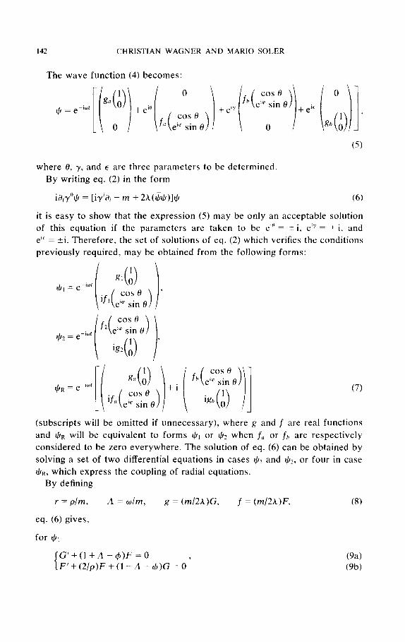
The wave function (4) becomes:

where 8, y, and E are three parameters to be determined.

By writing eq. (2) in the form

i&y’+ = [iy’ai - m + 2A(Ij$)]+ (6)

it is easy to show that the expression (5) may be only an acceptable solution

of this equation if the parameters are taken to be e” = -+ i, eiy = ? i, and

e If = ?i. Therefore, the set of solutions of eq. (2) which verifies the conditions

previously required, may be obtained from the following forms:

(7)

(subscripts will be omitted if unnecessary), where g and f are real functions

and IJJR will be equivalent to forms I/I~ or $,z when f. or fh are respectively

considered to be zero everywhere. The solution of eq. (6) can be obtained by

solving a set of two differential equations in cases r,!~, and IJQ, or four in case

IlrR, which express the coupling of radial equations.

By defining

r = plm, A = w/m, g = (m/2h)G, f = (mL’h)F, (8)

eq. (6) gives,

for *I G’+(l+A-4)F=O F’+(2/p)F+(l -A4 -$)G =O’

@a) (9b)


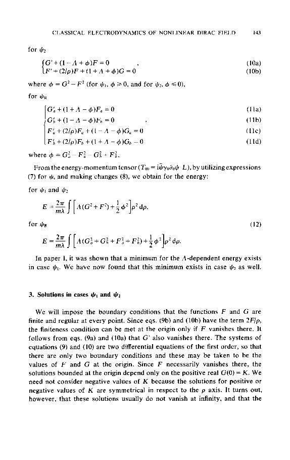
for Ccl2

{

G’+(l-A++)F=O F’+(2/p)F+(l+A +4)G =O’

where 4 = G2 - F* (for $J,, C#J 2 0, and for I&, 4 c 0),

for +R

1

Gb+(l+A-$)F, =0

G;,+(l-A -$)Fh =0 f

F:, + (2/p)F, + (1 - A - c$)G, = 0

Fb+(2/p)F,,+(l+A-$)G,=O

where+=Gi-Fi-Gi+Fi,

UW

(lob)

From the energy-momentum tensor (Too = i&y&&l;), by utilizing expressions

(7) for +, and making changes (S), we obtain for the energy:

for +i and I&

E=& mh

A(G2+F2)+;42 p’dp, I

(12)

E=k mh

A(G;+G;+F;+F;)++ p’dp. I

In paper I, it was shown that a minimum for the A-dependent energy exists in case 9,. We have now found that this minimum exists in case @I as well.

3. Solutions in cases JI, and I,&

We will impose the boundary conditions that the functions F and G are finite and regular at every point. Since eqs. (9b) and (lob) have the term 2F/p, the finiteness condition can be met at the origin only if F vanishes there. It follows from eqs. (9a) and (10a) that G’ also vanishes there. The systems of equations (9) and (10) are two differential equations of the first order, so that there are only two boundary conditions and these may be taken to be the values of F and G at the origin. Since F necessarily vanishes there, the solutions bounded at the origin depend only on the positive real G(0) = K. We need not consider negative values of K because the solutions for positive or negative values of K are symmetrical in respect to the p axis. It turns out, however, that these solutions usually do not vanish at infinity, and that the


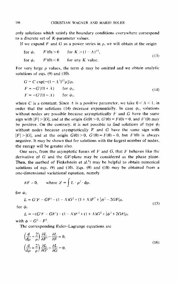
only solutions which satisfy the boundary conditions everywhere correspond

to a discrete set of K-parameter values.

If we expand F and G as a power series in p, we will obtain at the origin

for *I F’(0) > 0 for K > (1 - A )I”, (13)

for $I? F’(0) < 0 for any K value.

For very large p values, the term 4 may be omitted and we obtain analytic

solutions of eqs. (9) and (10).

G = C exp[-( 1 - .1’)“‘p]/p,

F = -G’/(l + A) for *I, (14) F = -G’/( 1 - 24) for *z,

where C is a constant. Since ii is a positive parameter, we take 0 < .I < I, in

order that the solutions (14) decrease exponentially. In case +r, solutions

without nodes are possible because asymptotically F and G have the same

sign with IFI > [Cl, and at the origin G(0) > 0, G’(0) = F(0) = 0, and F’(0) may

be positive. On the contrary, it is not possible to find solutions of type $2

without nodes because asymptotically F and G have the same sign with

JFI > IGJ, and at the origin G(O)>O, G’(0) = F(0) = 0, but F’(O) is always

negative. It may be shown that for solutions with the largest number of nodes,

the energy will be greater also.

One sees, from the asymptotic forms of F and G, that F behaves like the

derivative of G and the GF-plane may be considered as the phase plane.

Then, the method of Finkelstein et a1.6) may be helpful to obtain numerical

solutions of eqs. (9) and (10). Eqs. (9) and (10) may be obtained from a

one-dimensional variational equation, namely

X?=o, where Z’ = I

L . pz + dp,

for *I L=G’F-GF’-(l-A)G’+(l+.l)F’+&#+2GF/p,

for *?

L=-(G’F-GF’)-(1-A)F’+(1+A)G’+f~2+2GF/p,

with 4 = G’- F’.

The corresponding Euler-Lagrange equations are

(15)

(16)


By introducing into eqs. (16) the expressions (15) for L, we obtain eqs. (9) and (10). These equations may be regarded as describing the nonconservative motion of a point having position G and momentum F, because they depend explicitly on p (“time”). By dropping the term l/p from eqs. (9) and (lo), we obtain

for $1 G’+(l+A -&)F =O, F’+(l-A-c#J)G=O

for 42

G’+(l-A++)F=O F’+(l+A++)G=O’

(17)

which may be considered as the equations of a conservative motion. These equations can be also obtained from the lagrangian density (15) by omitting the term which contains p explicitly,

for $1 L,=G’F-GF’-(l-A)G2+(1+A)F2+~~*, (18)

for 42 i, = -(G’F - GF’) - (1 - A)F* + (1 + A)G* + ;c$‘,

and replacing these expressions of L in eq. (16). Now, we can construct a

pseudohamiltonian as follows

-H = (&aF’)F’ + (aL/aG’)G’ - i

obtaining

for $1 -H =(l-A)G*-(l+A)F*-&#?, (18)

for $2 -H= (I-A)F*-(l+A)G*-;$I*.

The equilibrium points of this motion (dH/aG = 0, aH/dF = 0) correspond to the trivial solution F = 0, G = 0 and to the special solutions

for $1 F = 0, G = ?(l - A)“*, (19)

for $2 G = 0, F = +(l -A)‘“.

These special solutions of eq. (17) are trivial solutions of the nonconservative motion in the case of I/RI (9) but not in the $2 case. In spite of this difference the same method is applicable in searching solutions of both cases. It is worth noting that if F and G are exchanged in eqs. (15), (17), (18), (19) and (20) in case I/Q, the equations obtained correspond to case $*.

The situation may be summarized more clearly by looking at the “phase plane FG”. The special solutions (18) will be represented by the points A,,

for $1 A, = (0, f (1 -A)“‘),

for $2 A, = (+(l -A)“‘, 0),


which are points of stable equilibria. The representative points of the con-

servative motion move on curves of constant H (18). The curve H = 0 is a

“figure-eight” through the origin. The curves H > 0 enclose the points A+ and

the origin, but the curves H < 0 enclose only one of the points A,. Thus the

origin is a saddle point. The representative point of the nonconservative

motion will terminate generally at one of the two stable equilibria points A +.

If the K value has been suitably taken, the representative point of the

nonconservative motion will arrive at the origin and the functions F and G

become physically normalizable with asymptotic exponential decay. Solutions

of eqs. (9) and (10) tend to solutions of eqs. (17) for large values of p, and we

know the equilibrium solutions of these equations.

Now, the technique for solving eqs. (9) and (10) numerically is found by

plotting the functions F and G against p (see fig. 1 for r/~, and fig. 2 for 4?). (A

more rigorous justification of this technique has been given for the nonlinear

scalar field by Finkelstein et al.‘).) Starting at p = 0 with G = K we obtain

solutions which oscillate asymptotically along the special functions (20) or

K K \

K, h \:, \ 0.G ‘(\ Az0.938 K.zO.96 K50.9075 yzO.85

-0.2 G:-JiTi G:=. _ --____ --’

Fig. 1. Shapes of the G functions obtained in case I,!J, for the physical solution (G) and for the

solutions G- and G corresponding to two inadequate values of K parameter (K, and K ).

A :0.93G5 K+=0.3700 K ~0.3282 K_=0.2900 0.4

F=rn E *_----__ .

0.2 .’ - A+ -_

Fig. 2. Shapes of the F functions obtained in case I& for the physical solution F and for the

solutions FA and F corresponding to two inadequate values of K parameter (K+ and K ).


else it will become a normalizable solution with asymptotic exponential decay (F-0, and G-0).

Similarly to case I,!Q, fig. 3 shows the existence of a minimum of the energy, located now at A = 0.937, K = 0.3281. The shapes obtained for F and G are in agreement with our considerations. (See fig. 4 for $12 and fig. 1 in paper I for $,.) The energy in case I/J~ is equal to 23.58(2m/m) MeV, approximately six times greater than the value obtained in case lJ12 (E = 3.76(2dmh) MeV). Since a fermion with rest energy about six times the proton energy is not known, & is not adequate to describe real particles.

Fig. 3. Variation of the energy with A in case $2.

Fig. 4. Shapes of the F and G functions obtained in case $2 corresponding to the physical

solution of minimum energy.


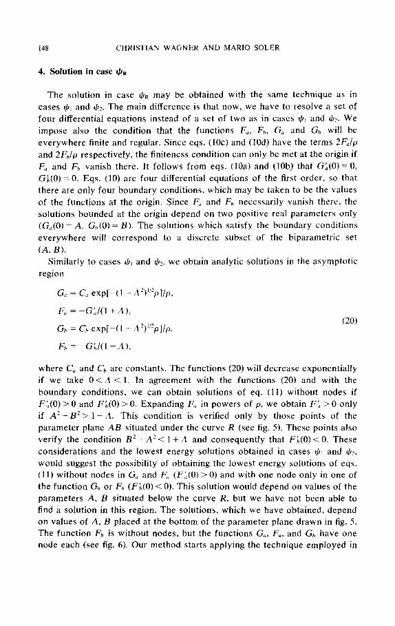
4. Solution in case JIR

The solution in case llrR may be obtained with the same technique as in

cases +, and +Q?. The main difference is that now, we have to resolve a set of

four differential equations instead of a set of two as in cases $, and &. We

impose also the condition that the functions F,, Fh, G, and GI, will be

everywhere finite and regular. Since eqs. (10~) and (10d) have the terms 2F,/p

and 2FJp respectively, the finiteness condition can only be met at the origin if

F, and F,, vanish there. It follows from eqs. (lOa) and (lob) that G:(O) = 0,

Gb(O) = 0. Eqs. (10) are four differential equations of the first order, so that

there are only four boundary conditions, which may be taken to be the values

of the functions at the origin. Since F,, and Fh necessarily vanish there, the

solutions bounded at the origin depend on two positive real parameters only

(G,(O) = A, G,,(O) = B). The solutions which satisfy the boundary conditions

everywhere will correspond to a discrete subset of the biparametric set

(A B). Similarly to cases 4, and I,& we obtain analytic solutions in the asymptotic

region

G, = C,, exp[-( 1 - A ‘)“‘p]/p,

F, = -GA/(1 + ,4),

GI, = Ct, exp[-(1 - z4’)“‘p~/p,

Ft, = -Gb/(l -A),

(20)

where C, and C,, are constants. The functions (20) will decrease exponentially

if we take 0 <A < 1. In agreement with the functions (20) and with the

boundary conditions, we can obtain solutions of eq. (11) without nodes if

F:(O) > 0 and FL(O) > 0. Expanding F, in powers of p, we obtain Fl, > 0 only

if A2 - B2 > 1 -A. This condition is verified only by those points of the

parameter plane AB situated under the curve R (see fig. 5). These points also

verify the condition B2 - A2 < 1 + A and consequently that FL(O) < 0. These

considerations and the lowest energy solutions obtained in cases 4, and Gz,

would suggest the possibility of obtaining the lowest energy solutions of eqs.

(11) without nodes in G, and F, (F:(O) > 0) and with one node only in one of

the function G,, or F,, (FL(O) < 0). This solution would depend on values of the

parameters A, B situated below the curve R, but we have not been able to

find a solution in this region. The solutions, which we have obtained, depend

on values of A, B placed at the bottom of the parameter plane drawn in fig. 5.

The function Fb is without nodes, but the functions G,, F,, and G,, have one

node each (see fig. 6). Our method starts applying the technique employed in

CLASSICAL

Fig. 5. Parametric plane

ELECTRODYNAMICS OF NONLINEAR DIRAC FIELD 149

020 B Q25 0.30

- 1.2

AB where it is shown the point corresponding to the physical solution obtained for A = 0.94 in case $R.

1

0.5

(

-0. :

A=l. 3772715

B=0.2057115

A=0.9&

Fig. 6. Shape of the G., GI,, F,, and Ft, functions obtained in case en and corresponding to the physical solution for A = 0.94.


cases 4, and I+!+ to solve eqs. (11). We can construct here also a pseudo-

hamiltonian for the conservative motion, whose equilibrium points will verify

the equations

G; + F; = 0, F;+G; =O,

which correspond to a saddle point, or

G;+F;= l-.2, F:+G; =O,

which correspond to a minimum point. The function Gt + Fi = I - .I is a

cylindrical surface in the three-dimensional space (Fhr G,,, p). We need not

consider the five-dimensional space (G,,, F,,, G,,, Fh, p) because for real

functions the condition Ft + Gz = 0 is equivalent to F,, = 0 and G,, = 0. This

cylindrical surface corresponds to the straight lines G = ?(l - LI)“Z in case 4,

and to F = +(l - ;I)“’ in case $2. The eqs. (11) define a curve in the (F,, G,,, p)

space. For large values of p this curve is a helix on the cylindrical surface. Its

pitch may change abruptly for some small changes in the values of the

parameters A, B. These abrupt changes allow us to draw the separation line

“S” over the parameter plane AB, which is thus divided in two parts (see fig.

5). For Points (A, B) very near to the curve S, G,, remains positive or negative

for very large values of p. We can have trouble with this second rule if we

consider points not very near to curve S. By using these two rules we can

suitably take a point of the parameter plane AB from which we will obtain a

normalizable solution of eqs. (11) with asymptotic exponential decay. With

A = 0.940, the suitable values are A = 1.377272 and B = 0.2OS712 (see fig. 3).

Since the minimum of energy will be about ten times greater than in case $I,,

this solution will be an inadequate “first step” for a fermion model.

Finally, it is interesting to note that for the three forms of the wave

function and independently of the values of m and 1, the self-interaction

energy contributes only a small fraction (l/10) compared with the energy

coming from terms that are also present in a linear theory. This percentage is

still smaller for large values of p. The main effect of the nonlinear terms is

therefore to bind the solutions at small distances and prevent them from

becoming infinite at the origin.

Appendix

We will now consider that in the case +, (7) the functions f and g are

complex.


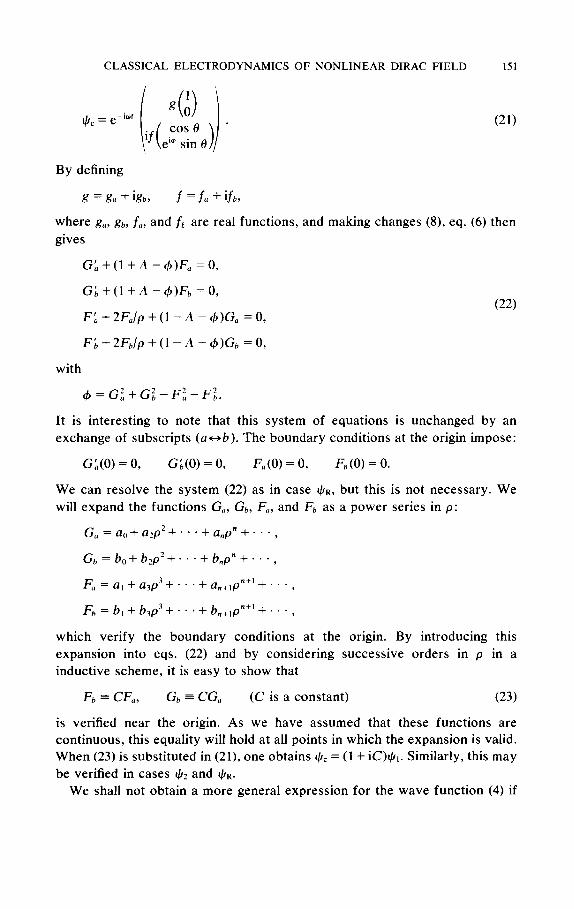
0 +c=e-i”’ if(e;o;z,) . r :I (21)

By defining

g = g, + igb, f =fo +ifb,

where g,, gb, fO, and ft are real functions, and making changes (8), eq. (6) then

gives

G;+(l+A -+)Fa =O,

Gb+(l+A--c))Fb=o,

Fb+2F,/p+(l-A-4)G, =O,

Fb+2Fb/p+(l-n-4)G,=O,

with

4 =G:+G:,-Ff,-F;.

(22)

It is interesting to note that this system of equations is unchanged by an

exchange of subscripts (a-b). The boundary conditions at the origin impose:

G:(O) = 0, Gb(0) = 0, F, (0) = 0, Fb (0) = 0.

We can resolve the system (22) as in case I,!+,, but this is not necessary. We

will expand the functions G,, Gb, F,, and Fb as a power series in p:

G,=ao+azp2+...+a,p”+...,

Gb=bo+b2p2+..*+b,p”+...,

F, = a, + a3p3 + . . . + a,+,~“+’ + . . . ,

Fb = b, + b3p3 + . . * + b,+,p”+’ + . . . ,

which verify the boundary conditions at the origin. By introducing this

expansion into eqs. (22) and by considering successive orders in p in a

inductive scheme, it is easy to show that

Fb = CF,, Gb = CG, (C is a constant) (23)

is verified near the origin. As we have assumed that these functions are

continuous, this equality will hold at all points in which the expansion is valid.

When (23) is substituted in (21), one obtains & = (1 + iC)4,. Similarly, this may

be verified in cases I/I? and I,!I~.

We shall not obtain a more general expression for the wave function (4) if


the radial functions are considered to be complex instead of real, because we

have just shown that this is equivalent to multiplying by an arbitrary phase.

References

1) See for example the review article by R. Jackiw, Rev. of Mod. Phys. 49 (1977) 681.

Other relevant recent works in this direction are A.M. Polyakov, Phys. Letters 59B (1975) 82,

and A.A. Belavin et al., Phys. Letters 59B (1975) 85, E.W. Mielke, Phys. Rev. Letters 39 (1977)

530, P. Vinciarelli, Phys. Rev. Letters 38 (1977) 1179, P. Sikivie and N. Weirs. Phys. Rev.

Letters 40 (1978) 1411, etc.

2) M. Soler, Phys. Rev. Dl (1970) 2766.

3) H. Weyl, Phys. Rev. 77 (1950) 699.

4) A.F. Raiiada and M. Soler, J. Math. Phys. 13 (1972) 671.

M. Soler, Phys. Rev. D8 (1973) 3424.

A.F. Ratiada and M. Soler, Phys. Rev. D8 (1973) 3430.

A.F. Rafiada et al., Phys. Rev. DIO (1974) 517.

5) Our notation will be:

where u’ are the Pauli metrices.

6) R. Finkelstein, R. Lelevier and M. Ruderman. Phys. Rev. 84 (1951) 326

Classical electrodynamics of a nonlinear Dirac field free solutions

Documents

Transcript of Classical electrodynamics of a nonlinear Dirac field free solutions