Superconducting Cavities for Circuit Quantum Electrodynamics
220
Superconducting Cavities for Circuit Quantum Electrodynamics A Dissertation Presented to the Faculty of the Graduate School of Yale University in Candidacy for the Degree of Doctor of Philosophy by Matthew James Reagor Dissertation Director: Professor Robert J. Schoelkopf December 2015
-
Upload
khangminh22 -
Category
Documents
-
view
0 -
download
0
Transcript of Superconducting Cavities for Circuit Quantum Electrodynamics

Superconducting Cavities forCircuit Quantum Electrodynamics
A DissertationPresented to the Faculty of the Graduate School
ofYale University
in Candidacy for the Degree ofDoctor of Philosophy
byMatthew James Reagor
Dissertation Director: Professor Robert J. Schoelkopf
December 2015

© 2015 by Matthew James ReagorAll rights reserved.
Superconducting Cavities forCircuit Quantum Electrodynamics
Matthew James Reagor2015
The components of a circuit Quantum Electrodynamics (cQED) system are mesoscopicand engineered. As a consequence, strong interactions are nearly automatic, making cQEDa viable platform for quantum information processing. However, strong interactions alsopersist to the unintended elements that originate from the engineering of any device. Thesespurious interactions decohere a cQED system and will ultimately limit the performance offuture superconducting quantum processors. This thesis explores novel architectures forcQED that eliminate decoherence. We leverage three-dimensional (3D) microwave cavitiesto shape resonant fields into low-loss configurations. Previously, such techniques haveresulted in highly coherent superconducting qubits. We extend this approach to realize anovel quantum memory for qubits based on superconducting cavity resonators. Our cavitymemory architecture exceeds millisecond lifetimes for superpositions that are written bya superconducting qubit to the memory. This type of device will enable future studiesof fault-tolerant quantum information processing with highly coherent, resource efficientmemory systems, as well as fundamental tests of quantum optical dynamics.

Contents
Contents iii
List of Figures vii
List of Tables x
Acknowledgements xi
Publication list xiii
1 Introduction 11.1 Overview of this thesis . . . . . . . . . . . . . . . . . . . . . . . . . . . 3
2 Circuit QED 52.1 Building blocks of cQED . . . . . . . . . . . . . . . . . . . . . . . . . . 6
2.1.1 The quantized circuit . . . . . . . . . . . . . . . . . . . . . . . 72.1.2 Gaussian states in an LC oscillator . . . . . . . . . . . . . . . . 102.1.3 Arbitrary classical drives on linear circuits . . . . . . . . . . . . . 13
2.2 Josephson junctions . . . . . . . . . . . . . . . . . . . . . . . . . . . . 152.2.1 Nonlinear inductance . . . . . . . . . . . . . . . . . . . . . . . . 162.2.2 Quantized Josephson effects . . . . . . . . . . . . . . . . . . . . 18
2.3 Quantum Josephson circuits . . . . . . . . . . . . . . . . . . . . . . . . 182.3.1 Black Box Quantization of a Josephson circuit . . . . . . . . . . 192.3.2 Transmon artificial atoms . . . . . . . . . . . . . . . . . . . . . 202.3.3 Driving a transmon atom . . . . . . . . . . . . . . . . . . . . . 212.3.4 Exciting a transmon atom . . . . . . . . . . . . . . . . . . . . . 242.3.5 Selection rules and multi-photon transitions . . . . . . . . . . . . 28
iii

iv
2.4 Coupling quantum circuits . . . . . . . . . . . . . . . . . . . . . . . . . 292.4.1 Black Box Quantization for many modes . . . . . . . . . . . . . 31
2.5 Detecting the state of a transmon . . . . . . . . . . . . . . . . . . . . . 362.5.1 Selection rules for many-wave mixing . . . . . . . . . . . . . . . 39
3 Quantum information in harmonic oscillators 423.1 Photons carrying classical bits . . . . . . . . . . . . . . . . . . . . . . . 433.2 State tomography of an oscillator . . . . . . . . . . . . . . . . . . . . . 45
3.2.1 Fock state distribution . . . . . . . . . . . . . . . . . . . . . . . 463.2.2 Husimi Q functions . . . . . . . . . . . . . . . . . . . . . . . . 473.2.3 Wigner tomography . . . . . . . . . . . . . . . . . . . . . . . . 513.2.4 Flying state tomography . . . . . . . . . . . . . . . . . . . . . . 54
3.3 Dispersive control . . . . . . . . . . . . . . . . . . . . . . . . . . . . . 583.3.1 QCMap gate . . . . . . . . . . . . . . . . . . . . . . . . . . . . 583.3.2 SNAP gate . . . . . . . . . . . . . . . . . . . . . . . . . . . . . 60
3.4 Decoherence in an oscillator . . . . . . . . . . . . . . . . . . . . . . . . 623.4.1 Energy decay . . . . . . . . . . . . . . . . . . . . . . . . . . . . 633.4.2 Phase noise . . . . . . . . . . . . . . . . . . . . . . . . . . . . 66
3.5 Quantum error correction on cat-codes . . . . . . . . . . . . . . . . . . 673.5.1 Cyclic photon-loss . . . . . . . . . . . . . . . . . . . . . . . . . 67
4 Photon boxes for cQED 714.1 Quantizing a distributed mode . . . . . . . . . . . . . . . . . . . . . . . 714.2 Quality factors and participation ratios . . . . . . . . . . . . . . . . . . 74
4.2.1 External loss . . . . . . . . . . . . . . . . . . . . . . . . . . . . 764.2.2 Dielectric loss . . . . . . . . . . . . . . . . . . . . . . . . . . . 774.2.3 Conductor loss . . . . . . . . . . . . . . . . . . . . . . . . . . . 794.2.4 Contact resistance . . . . . . . . . . . . . . . . . . . . . . . . . 804.2.5 Summary of loss mechanisms . . . . . . . . . . . . . . . . . . . 81
4.3 Planar resonators . . . . . . . . . . . . . . . . . . . . . . . . . . . . . . 824.3.1 Resonant modes of a CPW . . . . . . . . . . . . . . . . . . . . 824.3.2 Input-output coupling . . . . . . . . . . . . . . . . . . . . . . . 844.3.3 Planar transmons . . . . . . . . . . . . . . . . . . . . . . . . . 844.3.4 Losses . . . . . . . . . . . . . . . . . . . . . . . . . . . . . . . 85
4.4 Rectangular cavity resonators . . . . . . . . . . . . . . . . . . . . . . . 864.4.1 Resonant modes . . . . . . . . . . . . . . . . . . . . . . . . . . 874.4.2 Input-output coupling . . . . . . . . . . . . . . . . . . . . . . . 884.4.3 3D transmon . . . . . . . . . . . . . . . . . . . . . . . . . . . . 934.4.4 Losses . . . . . . . . . . . . . . . . . . . . . . . . . . . . . . . 95
4.5 Cylindrical cavity resonators . . . . . . . . . . . . . . . . . . . . . . . . 974.5.1 Resonant modes . . . . . . . . . . . . . . . . . . . . . . . . . . 984.5.2 Input-output coupling . . . . . . . . . . . . . . . . . . . . . . . 100

v
4.5.3 Losses . . . . . . . . . . . . . . . . . . . . . . . . . . . . . . . 1024.5.4 Hurdles to transmon integration . . . . . . . . . . . . . . . . . . 103
4.6 Coaxial λ/4 resonators . . . . . . . . . . . . . . . . . . . . . . . . . . . 1044.6.1 Resonant modes . . . . . . . . . . . . . . . . . . . . . . . . . . 1044.6.2 Input-output coupling . . . . . . . . . . . . . . . . . . . . . . . 1064.6.3 Integrating a transmon . . . . . . . . . . . . . . . . . . . . . . . 1064.6.4 Losses . . . . . . . . . . . . . . . . . . . . . . . . . . . . . . . 109
4.7 Summary of modes and quality factors . . . . . . . . . . . . . . . . . . 110
5 Measuring resonators and transmons 1125.1 Linear resonator experiments . . . . . . . . . . . . . . . . . . . . . . . 112
5.1.1 Surface preparation . . . . . . . . . . . . . . . . . . . . . . . . 1135.1.2 Resonator measurement setup . . . . . . . . . . . . . . . . . . . 1165.1.3 Extracting quality factors . . . . . . . . . . . . . . . . . . . . . 1165.1.4 Power dependence . . . . . . . . . . . . . . . . . . . . . . . . . 1215.1.5 Temperature dependence . . . . . . . . . . . . . . . . . . . . . 124
5.2 Transmon measurements . . . . . . . . . . . . . . . . . . . . . . . . . . 1295.2.1 Fabrication . . . . . . . . . . . . . . . . . . . . . . . . . . . . . 1305.2.2 Measurement setup . . . . . . . . . . . . . . . . . . . . . . . . 1305.2.3 Control signals . . . . . . . . . . . . . . . . . . . . . . . . . . . 1315.2.4 Readout signals . . . . . . . . . . . . . . . . . . . . . . . . . . 1335.2.5 JPC-backed dispersive readout . . . . . . . . . . . . . . . . . . 1355.2.6 Spectroscopy . . . . . . . . . . . . . . . . . . . . . . . . . . . . 1375.2.7 Rabi oscillations . . . . . . . . . . . . . . . . . . . . . . . . . . 1385.2.8 Lifetime . . . . . . . . . . . . . . . . . . . . . . . . . . . . . . 1395.2.9 Coherence . . . . . . . . . . . . . . . . . . . . . . . . . . . . . 139
6 Characterizing near-millisecond coherence in a cQED oscillator 1416.1 Dispersive coupling . . . . . . . . . . . . . . . . . . . . . . . . . . . . . 141
6.1.1 Number-splitting spectroscopy . . . . . . . . . . . . . . . . . . . 1426.1.2 Time-domain techniques . . . . . . . . . . . . . . . . . . . . . . 143
6.2 Classical energy decay rate . . . . . . . . . . . . . . . . . . . . . . . . . 1456.2.1 Calibrating control pulses . . . . . . . . . . . . . . . . . . . . . 1456.2.2 Coherent state κ experiment . . . . . . . . . . . . . . . . . . . 146
6.3 Coherence experiments . . . . . . . . . . . . . . . . . . . . . . . . . . . 1486.3.1 Oscillator T1 . . . . . . . . . . . . . . . . . . . . . . . . . . . . 1486.3.2 Oscillator T2 . . . . . . . . . . . . . . . . . . . . . . . . . . . . 151
6.4 Qubit-induced decoherence . . . . . . . . . . . . . . . . . . . . . . . . 1536.4.1 Reverse-Purcell effects . . . . . . . . . . . . . . . . . . . . . . . 1546.4.2 Testing the reverse Purcell effect . . . . . . . . . . . . . . . . . 1576.4.3 Shot-noise dephasing in cQED . . . . . . . . . . . . . . . . . . . 160
6.5 Outlook for resonator quantum memories . . . . . . . . . . . . . . . . . 164
vi
7 Conclusion 1667.1 Continuing Schoelkopf’s Law . . . . . . . . . . . . . . . . . . . . . . . 1667.2 Controlling quantum states in resonators . . . . . . . . . . . . . . . . . 168
Bibliography 170
Appendices 188
A Arbitrary classical drives on linear circuits 188
B Superpositions with SNAP 191
C Evanescent coupling to resonators 193
D Integrals and participation ratios for cylindrical cavities 197D.1 TMnml modes . . . . . . . . . . . . . . . . . . . . . . . . . . . . . . . 197D.2 TEnml modes . . . . . . . . . . . . . . . . . . . . . . . . . . . . . . . . 202
E BCS Calculations 204
Copyright Permissions 206

List of Figures
2 Circuit QED2.1 Quantum harmonic oscillators . . . . . . . . . . . . . . . . . . . . . . . 72.2 Energy levels of the quantum harmonic oscillator . . . . . . . . . . . . . 92.3 Photon number statistics of coherent states . . . . . . . . . . . . . . . . 122.4 Effect of an arbitrary drive on a damped oscillator . . . . . . . . . . . . 152.5 Josephson effect as a circuit element . . . . . . . . . . . . . . . . . . . 172.6 Quantizing the Josephson LC oscillator . . . . . . . . . . . . . . . . . . 202.7 Classical dressing of a linear circuit . . . . . . . . . . . . . . . . . . . . 302.8 Black box quantization of many modes . . . . . . . . . . . . . . . . . . 322.9 Cross-Kerr nonlinear effects . . . . . . . . . . . . . . . . . . . . . . . . 342.10 Reading out the state of a transmon . . . . . . . . . . . . . . . . . . . 382.11 Josephson junction as a scattering site . . . . . . . . . . . . . . . . . . 40
3 Quantum information in harmonic oscillators3.1 Phase shift-keying (PSK) of classical signals . . . . . . . . . . . . . . . 443.2 Quantifying the statistics of a resonator state . . . . . . . . . . . . . . . 483.3 Husimi Q distribution of resonator states . . . . . . . . . . . . . . . . . 503.4 Two techniques for measuring parity . . . . . . . . . . . . . . . . . . . . 523.5 Wigner tomography in cQED . . . . . . . . . . . . . . . . . . . . . . . 553.6 Creating nonclassical states via SNAP . . . . . . . . . . . . . . . . . . . 623.7 Cat-code logical qubit encoding . . . . . . . . . . . . . . . . . . . . . . 69
4 Photon boxes for cQED4.1 Black box quantization of a distributed mode . . . . . . . . . . . . . . . 734.2 General loss mechanisms for a resonator . . . . . . . . . . . . . . . . . . 754.3 Treating external dissipation . . . . . . . . . . . . . . . . . . . . . . . . 77
vii

viii
4.4 Planar resonators and transmons . . . . . . . . . . . . . . . . . . . . . 834.5 Experimental realization of planar circuit elements . . . . . . . . . . . . 864.6 Rectangular cavities and the 3D transmon . . . . . . . . . . . . . . . . 884.7 Input-output coupling for rectangular cavities . . . . . . . . . . . . . . . 894.8 Perturbation of surface currents induced by substrate . . . . . . . . . . . 964.9 Cylindrical TE011 resonator . . . . . . . . . . . . . . . . . . . . . . . . 1004.10 Input-output coupling for cylindrical cavities . . . . . . . . . . . . . . . 1014.11 Coaxial λ/4 resonator . . . . . . . . . . . . . . . . . . . . . . . . . . . 1054.12 Assembling a coaxial quarter-wave cQED device . . . . . . . . . . . . . 107
5 Measuring resonators and transmons5.1 Surface preparation of superconducting cavities . . . . . . . . . . . . . . 1145.2 Calibrating the etch rate of Aluminum Etch A . . . . . . . . . . . . . . 1155.3 Experimental schematic for resonator testing . . . . . . . . . . . . . . . 1175.4 Picture of resonator payload . . . . . . . . . . . . . . . . . . . . . . . . 1185.5 Shunt resonances along a transmission line . . . . . . . . . . . . . . . . 1195.6 Fitting quality factors on the complex plane . . . . . . . . . . . . . . . . 1215.7 Power dependence of two cavity resonators . . . . . . . . . . . . . . . . 1235.8 BCS theory for surface impedance of a superconductor . . . . . . . . . . 1255.9 Temperature dependence of two superconducting resonators . . . . . . . 1275.10 Fitting temperature dependence to BCS theory . . . . . . . . . . . . . . 1285.11 Observed quality factors compared to BCS theory . . . . . . . . . . . . 1295.12 Low-temperature schematic for cQED device testing . . . . . . . . . . . 1325.13 Room-temperature schematic for modulation and demodulation . . . . . 1335.14 Picture of cQED setup . . . . . . . . . . . . . . . . . . . . . . . . . . . 1345.15 Dispersive readout signal . . . . . . . . . . . . . . . . . . . . . . . . . . 1365.16 JPC tuneup and gain curve . . . . . . . . . . . . . . . . . . . . . . . . 1375.17 Transmon spectroscopy . . . . . . . . . . . . . . . . . . . . . . . . . . 1385.18 Transmon qubit characterization measurements . . . . . . . . . . . . . . 140
6 Characterizing near-millisecond coherence in a cQED oscillator6.1 Number-splitting spectroscopy . . . . . . . . . . . . . . . . . . . . . . . 1436.2 Time-domain χ measurement . . . . . . . . . . . . . . . . . . . . . . . 1446.3 Calibrating cavity displacement pulses . . . . . . . . . . . . . . . . . . . 1466.4 Energy decay of a qubit-coupled resonator . . . . . . . . . . . . . . . . 1476.5 Preparation of nonclassical states via SNAP . . . . . . . . . . . . . . . . 1506.6 T1 decay of an |1〉 Fock state . . . . . . . . . . . . . . . . . . . . . . . 1516.7 Theoretical analysis of pure dephasing in a resonator . . . . . . . . . . . 1536.8 T2 decay of an |0〉 and |1〉 superposition state . . . . . . . . . . . . . . 1546.9 Capturing Purcell effects with linear LC circuits . . . . . . . . . . . . . . 1556.10 Temperature dependence of a cQED system . . . . . . . . . . . . . . . 1586.11 Revealing reverse-Purcell effects in a resonator . . . . . . . . . . . . . . 159

ix
6.12 Shot-noise dephasing in cQED . . . . . . . . . . . . . . . . . . . . . . . 1616.13 Increasing qubit population with weak drives . . . . . . . . . . . . . . . 1626.14 Revealing shot-noise dephasing of a cQED resonator . . . . . . . . . . . 163
7 Conclusion7.1 Schoelkopf’s Law for the coherence times of circuits . . . . . . . . . . . 167
B AppendixB.1 Python code for simulating SNAP processes . . . . . . . . . . . . . . . 192
C AppendixC.1 Measured scaling of external coupling for rectangular cavity . . . . . . . 194C.2 Loop coupling scheme for cylindrical cavities . . . . . . . . . . . . . . . 195C.3 Measured scaling of external coupling for cylindrical cavity . . . . . . . . 196
E AppendixE.1 Mathematica code for evaluating the BCS surface impedance . . . . . . 205

List of Tables
4.1 Predicted and extracted parameters for the full device device Hamiltonian. 1084.2 Resonant modes and quality factors for high purity aluminum. . . . . . . 111
C.1 Propagation constants for the lowest three sub-cutoff modes of a pincoupled circular waveguide. . . . . . . . . . . . . . . . . . . . . . . . . 194
C.2 Propagation constants for for the lowest three sub-cutoff modes of a loopcoupled circular waveguide. . . . . . . . . . . . . . . . . . . . . . . . . 195
x

Acknowledgements
In compiling these acknowledgments, I am humbled by the cast of people I have beenfortunate enough to call friends. I owe a great deal to Robert Schoelkopf. As my
thesis advisor, Rob introduced me to superconductors, microwave circuits, and low-noisemeasurements. Rob has taught me how to ask questions, how to simplify problems, andhow to work out the details of an experiment with the big picture in focus.
I am indebted to Michel Devoret for being so generous with his time and brilliance.Walking into Michel’s office has always been a personal thrill, and walking out has alwaysmeant a wonderful, fleeting sense of enlightenment. Daniel Prober has been a mentorto me since my first day in Becton. His active fostering of the best possible cultureamong the research groups here has been instrumental to all of our achievements. Luigi
Frunzio has a genuine passion for teaching and made the work in this thesis possible.Without Luigi, I would have ended up doing theoretical physics. I would then have beenlucky to know Liang Jiang. Liang can explain difficult concepts with remarkable ease,and his creativity shines through in every conversation. In addition, I would like to thank allof the above colleagues, as well as Konrad Lehnert, for participating in the preparationof this thesis.
I would like to thank Wolfgang Pfaff for teaching me how to run an experimentwith thoughtfulness and organization; how to write and manage useful code; how toillustrate beautiful plots and figures; and how to have a good time doing it all. Workingalongside Wolfgang has been an absolute pleasure for the last few years. When Reinier
Heeres arrived at Yale, he completely disrupted the software infrastructure of the lab,and I feel lucky to have learned cQED experiments in the post-Heeres era. Besides hisdepth of knowledge from software to fabrication and more, Reinier also possesses an honest
xi

ACKNOWLEDGEMENTS xii
frankness that has elevates discourse. Jacob Blumoff and Kevin Chou have alwaysthe first people I turn to when I needed a second opinion, on anything. They are awesomepeople to solve problems with. Few people have had as much impact on how I thinkabout Josephson junctions and quantum mechanics as Zaki Leghtas and Gerhard
Kirchmair. It has been inspiring to work with folks who approached concepts (that Ithought I already knew) with a radically different framework.
Uri Vool and Michael Hatridge were always happy to listen to new results,provide feedback, and give encouragement too, which has picked me up many timesthroughout this thesis. Teresa Brecht has always had aptitude for hard technicalproblems. Her dedication and skill is inspiring. I would especially like to thank ‘Uncle’Chris Axline who has saved my dogs from trouble on an uncountable number ofoccasions. He has also been a remarkable labmate (e.g. Chris built an emergency operatingsystem for the physical infrastructure of our building). In addition, Chris has contributedhis a phenomenal talent on various hardware collaborations. Eric Holland has beena friend who I can talk through any situation with, and I am truly indebted to him forlistening to ups and downs and helping me keep a level head. Maria Rao and Giselle
DeVito have made the fourth floor of Becton feel like a second home. I have sharedthat home with too many great colleagues for me to recognize all of their importantcontributions here.
I had the good fortune to spend time with Eric Dufresne, Joseph Zinter, Jean
Zheng, and Larry Wilen, as well as many talented staff members, in my capacityas a teaching fellow in the Center for Engineering Innovation and Design. Piggybackingoff their awesome classes, I have worked on problems from gastrointestinal surgery toregulating climate for leaf-cutter ants. Those experiences have shaped my character inprofound ways.
Finally, I would like to thank my family for their love and support. My wife, Jennifer
Reagor, has been a part of this journey since its beginning. Her support has been aconstant source of joy throughout.

Publication list
This thesis is based in part on the following publications:
1. H. Paik, D. I. Schuster, L. S. Bishop, G. Kirchmair, G. Catelani, A. P. Sears, B. R.Johnson, M. J. Reagor, L. Frunzio, L. I. Glazman, S. M. Girvin, M. H. Devoret, andR. J. Schoelkopf, ‘Observation of High Coherence in Josephson Junction QubitsMeasured in a Three-Dimensional Circuit QED Architecture,’ Physical Review Letters107, 240501 (2011),
2. M. Reagor, H. Paik, G. Catelani, L. Sun, C. Axline, E. Holland, I. M. Pop, N. A.Masluk, T. Brecht, L. Frunzio, M. H. Devoret, L. Glazman, and R. J. Schoelkopf,‘Reaching 10 ms single photon lifetimes for superconducting aluminum cavities,’Applied Physics Letters 102, 192604 (2013).
3. Z. Leghtas, S. Touzard, I. M. Pop, A. Kou, B. Vlastakis, A. Petrenko, K. M. Sliwa,A. Narla, S. Shankar, M. J. Hatridge, M. Reagor, L. Frunzio, R. J. Schoelkopf, M.Mirrahimi, and M. H. Devoret, ‘Confining the state of light to a quantum manifoldby engineered two-photon loss,’ Science 347, 853 (2015).
4. E. T. Holland, B. Vlastakis, R. W. Heeres, M. J. Reagor, U. Vool, Z. Leghtas,L. Frunzio, G. Kirchmair, M. H. Devoret, M. Mirrahimi, and R. J. Schoelkopf,‘Single-photon Resolved Cross-Kerr Interaction for Autonomous Stabilization ofPhoton-number States,’ In press at Physical Review Letters (2015).
5. T. Brecht, M. Reagor, Y. Chu, W. Pfaff, C. Wang, L. Frunzio, M. H. Devoret, and R.J. Schoelkopf, ‘Demonstration of Superconducting Micromachined Cavities,’ AppliedPhysics Letters 107, 192603 (2015).
6. M. Reagor, W. Pfaff, C. Axline, R. W. Heeres, N. Ofek, K. Sliwa, E. Holland, C.Wang, J. Blumoff, K. Chou, M. J. Hatridge, L. Frunzio, M. H. Devoret, L. Jiang,and R. J. Schoelkopf, ‘Quantum Memory with Near-Millisecond Coherence in CircuitQED,’ ArXiv e-prints (2015), 1508.05882 [quant-ph].
xiii

CHAPTER 1
Introduction
Heike Kamerlingh Onnes began seeking applications for superconductivity soon afterhe discovered the effect. Kamerlingh Onnes believed that his coils, which carried
electrical currents without resistance, could act as permanent magnets of arbitrarily largestrength [1]. Such magnets could in turn spawn new discoveries and technologies. WhenKamerlingh Onnes’s coils were looped on themselves, they could sustain currents at near-Ampere levels long after their generation. For a demonstration at London’s Royal Society,Kamerlingh Onnes’s coils were shown to be strongly magnetic after being transported byplane (in liquid helium) from Kamerlingh Onnes’s Leiden laboratory, where the currentshad been generated [2]. Yet, Onnes’s magnets would always decay, eventually. To hisfrustration, Kamerlingh Onnes found that his superconducting coils had finite current-carrying capacity too, breaking-down sharply at some threshold currents. For the remainderof his career, Kamerlingh Onnes made incremental progress with increasingly pure samplesand new superconductors toward his goal of more powerful superconducting magnets [1].
We celebrated the 100th anniversary of Kamerlingh Onnes’s discovery in 2011. Werecognize now that Kamerlingh Onnes’s threshold currents were critical magnetic fieldeffects. These would only be explained after World War I, and Kamerlingh Onnes’sretirement. The vision of useful superconducting magnets was eventually fulfilled though:they are now found in most hospitals, where they enable life-saving MRI scans.
1

CHAPTER 1. INTRODUCTION 2
Superconductivity is a great example of a quantum mechanical phenomenon thatcan be used for improving a classical technology. The effect’s quantum descriptioncan be completely ignored in most applications. Engineers can swap copper wire forsuperconducting wire with minor woes. Indeed, Onnes was ignorant of, but confident in, thequantum mechanical description of supercurrents [2]. For emerging quantum technologies,such as quantum-enhanced metrology, cryptography, or computational systems, the end-user must purposefully control the quantum evolution of system.
In many ways, makers of quantum technologies benefit from more than a centuryof quantum mechanics. We take for granted that the ‘spookiness’ [3] has largely beenremoved from the conversation. However, the path to universal quantum computationtraverses untested physics∗. No experiment has yet shown that the fundamental tenetsquantum error correction are correct [4], and further, that they will persist to the logicalerror levels required for large quantum algorithms [5]. Already though, the pursuit ofquantum information science has inspired new ways of thinking about other physicalsystems, such as the interplay of quantum error correction and black holes [6].
In many ways, this thesis continues in Kamerlingh Onnes’s tradition. We are stillfabricating superconducting circuits and finding new techniques to extend the persistenceof their currents. There are a few key differences though. For one, Kamerlingh Onnes coilshad an inductance of nearly 10 mH. They thus sustained flux of approximately 10 mWb, ortwelve orders of magnitude larger than the magnetic flux quantum (h/2e ≈2 fWb), whichsets the scale of most experiments on quantum circuits. A second, crucial difference hereis that at these small excitation levels, circuits can oscillate with many phases at once,quantum mechanically.
This thesis concerns the onset of quantum effects in circuits and how they may beleveraged to take precision measurements of quantum processes and for performing quantumcomputation. In particular, we argue that harmonic oscillators can be remarkable objectsand demonstrate their application as coherent quantum memories for superconductingcircuits.
∗ Though, perhaps it is encouraging that Helium was only discovered on Earth a decade after KamerlinghOnnes began his pursuit of absolute zero.

1.1. OVERVIEW OF THIS THESIS 3
1.1 Overview of this thesis
We see how circuits can behave quantum mechanically in Chapter 2. We find that purelylinear circuit elements are relatively boring objects, beyond the existence of a noisy groundstate in these systems. However, adding nonlinearity to a resonant circuit gives it color [7].Superconducting circuits can acquire strong nonlinearities from the Josephson effect [8].We present a modern, detailed description of the arguably simplest Josephson quantumcircuit, the transmon [9, 10]. By examining the response of this circuit to resonant anddetuned drives, we show how a transmon can be treated as an artificial atom. Finally, weshow how coupled Josephson circuits can lead to an interesting conditional nonlinearitythat is also a hallmark of Cavity Quantum Electrodynamics (CQED) [11].
Motivated by the existence of nonlinear coupling, we show how otherwise-linear circuitscan be remarkable quantum objects in Chapter 3. Linearity provides the means to excitemany degrees of freedom in these systems at once, and each quanta of energy in the circuitadds new capacity for quantum information [12, 13]. We describe how such systems canbe measured and controlled via a conditional nonlinearity. The consequence of decoherencemechanisms in these systems is also important. We argue that particular states of linearcircuits could be used to defeat these loss mechanisms with an oscillator-based scheme forquantum error correction.
Next, we study the physical realization of these circuits in Chapter 4, consideringfour types of linear resonators in detail: coplanar transmission line resonators, rectangularwaveguide cavities, cylindrical waveguide cavities, and coaxial λ/4 cavities. We presenteach resonant mode structures and sensitivity to various loss mechanisms to understandits dissipation. As architectures for implementing circuit QED, we weigh the benefits andtrade-offs of each system. We conclude the chapter with the design of a robust cavityquantum memory, based on one of these resonators.
In Chapter 5, we discuss the experimental techniques for the individual design, fab-rication, and characterization of these circuit elements. We provide details on howsuperconducting cavity resonators are prepared in order to minimize their dissipation. Then,we describe the techniques for extracting the resonator’s quality from circuit-networkanalysis. Finally, we present an overview of how transmons are fabricated and measured.
Putting all of these ideas together, this thesis culminates in the experimental realizationof a transmon strongly coupled to a highly coherent cavity quantum memory, Chapter 6.We describe the calibration and characterization of the coupled system. The chapter
1.1. OVERVIEW OF THIS THESIS 4
includes measurement techniques for extracting of the cavity’s lifetime and coherence. Inparticular, we trace two important decoherence effects in the cavity to the transmon. Theresults in this chapter pave the way for implementing many of the ideas in Chapter 3.
We conclude this thesis, Chapter 7, with an outlook on coherence in cQED and futureexperiments with these systems. In particular, we consider leveraging the full atom-likecapabilities of transmons, as described in Chapter 2, as an opportunity to achieve moreprecise control over nearly-linear, highly coherent quantum circuits.

CHAPTER 2
Circuit QED
Circuit Quantum Electrodynamics (cQED) is a toolbox for implementing nontrivialquantum circuits that can be precisely designed and controlled. We begin this chapter
by putting the quantum mechanics of circuits on solid theoretical footing. We first describehow the circuit operators of voltage and flux can be quantized. Then, the theoreticalframework of the Josephson effect and its realization as a nonlinear circuit element isintroduced. Finally, we show how circuits coupled with Josephson elements can achieveQED effects.
This chapter benefits from a long history of excellent theses and pedagogical reviewson the subject of Josephson quantum circuits. In particular, the beginning of this chapterclosely follows the seminal work by Devoret [7] and especially the recent treatment byGirvin [14]. We rely on this foundation to advance a modern description of QED as anatural consequence the Josephson effect beginning in Section 2.3.2. By treating ourcQED system as a ‘Black Box’ [10], we are able to describe driven, coupled, nonlinear,quantum circuits with a single framework. The consequence (Section 2.4) is an intuitiveset of quantum behaviors and ‘selection rules’ for a circuit that can potentially possessmany degrees of freedom.
In order to explore the rich behavior of a single cQED system (an otherwise-linearcircuit with one Josephson element), this chapter does not review the many other types of
5

2.1. BUILDING BLOCKS OF CQED 6
quantum circuits or superconducting qubits in detail. For this purpose, we refer the readerto the reviews by Clarke and Wilhelm [15] and also the review by Devoret and Schoelkopf[16].
2.1 Building blocks of cQED
Circuits made of capacitors and inductors have equivalent descriptions in mechanicalsystems of masses and springs. We use that analogy throughout this section to justify ourintuition and make connections to other experimental techniques. For instance, voltage(V ) and flux (Φ) are collective phenomena. Typically in a circuit, a countless number ofcharge carriers generate our measured V or Φ. Fortunately, we are able to abstract awaythe microscopic forces that act on these solid-state charge carriers. This is analogous totreating a many-atom chunk of material as a single mass with a single momentum: as longas the inter-mass dynamics (lattice vibrations) occur at a sufficiently high frequency, wecan approximate these modes to be their ground state. Indeed, for aluminum circuits, theequivalent modes (plasma oscillations of free charge carriers) occur at frequencies aboveω/2π & 1015 Hz [17], five orders of magnitude higher frequencies than we consider here inthis thesis. The collective motion approximation is therefore well justified.
Superconductivity plays the vital role of suppressing dissipation in our circuits. Perhapsmore importantly, an ideal superconductor also gives us access to a dissipationless nonlinearcircuit element, which we describe in Section 2.2. In both of these cases, the gap of thesuperconductor (∆) gives us another ground state to consider, allowing more rigor to thecollective motion approximation [18]. The gap of our circuit’s superconductor also sets alimit to the temperatures and excitation energies that can be used [18]. The frequenciesassociated with the break down of superconductivity are much smaller than the onset ofplasma oscillations considered above. When working with aluminum for instance, drivesabove ω/2π & 2∆/h (≈ 80− 100GHz for aluminum) can efficiently excite quasiparticlesabove the gap.
Our operating frequencies are bounded below by the requirement that our resonantcircuits be in their quantum mechanical ground states. To achieve a Boltzmann factorsuppression of the first excited state to approximately one percent, we require then thatω/2π & 5kBT . At the operating temperatures of a commercial dilution refrigerator(T ∼ 20mK), that requirement translates to ω/2π & 2GHz. These considerationstherefore place our quantum circuits squarely in the microwave domain.

2.1. BUILDING BLOCKS OF CQED 7
LC
k
m
ω = LC1
ω = km
(a) (b)
Figure 2.1: Quantum harmonic oscillators. (a) An electrical harmonic oscillator isconstructed by placing a capacitor (C) in parallel with an inductor (L). The conjugatevariables that describe the resulting oscillation are the charge on the capacitor Q and fluxthrough the inductor Φ. The natural frequency of this oscillator is related to these two circuitelements by ω = 1/
√LC. (b) The analogous mechanical circuit to the LC oscillator is a
simple mass-spring system with mass m and inverse-spring constant k−1. In this oscillator,the displacement of the spring x and the momentum of the mass p form the equivalentconjugate variables to the system as charge and flux in the electrical circuit. The mechanicaloscillator has the resonant frequency ω =
√k/m.
2.1.1 The quantized circuit
To quantize a circuit we proceed in the canonical fashion [7, 14] by finding a Hamiltonianfor the system and its conjugate variables, which will become our quantum operators.The foundational circuit to this thesis is the linear oscillator (Fig. 2.1). This circuitcombines a capacitor (C) in parallel with an inductor (L). On resonance, energy sloshesbetween a charging energy (EC = Q2/2C) and an inductive energy (EL = Φ2/2L). Forthe mass-spring system, energy likewise oscillates between kinetic energy (p2/2m) andpotential energy (x2/2k−1). Combining the circuit’s kinetic energy (EC) and potentialenergy (EL) terms to form a Lagrangian [14] gives
L =Q2
2C− Φ2
2L. (2.1)

2.1. BUILDING BLOCKS OF CQED 8
Because these elements share a node in the circuit, we can use the flux-voltage relation [7]
Φ(t) ≡∫ t
−∞V (τ)dτ =
∫Q(τ)
Cdτ (2.2)
to rewrite the charging energy as
L =CΦ2
2− Φ2
2L. (2.3)
We recognize that flux through the inductor (Φ = LQ) is the conjugate variable of charge[14], since
δLδΦ
= LQ = Φ. (2.4)
Therefore, we have a classical Hamiltonian for this circuit that is
H = ΦQ− L =Φ2
2L+Q2
2C. (2.5)
Now, we are now ready convert these variables to quantum mechanical operators (e.g.Φ⇒ Φ) and the Hamiltonian as well (H ⇒ H). Additionally, we can factor Equation 2.5,using
x2 + y2 = (x+ ıy)(x− ıy)− ı [x, y] (2.6)
to eventually simplify our circuit’s description, now giving
H =
(Φ√2L
+ ıQ√2C
)(Φ√2L− ı Q√
2C
)− ı
2√LC
[Q, Φ
]. (2.7)
The conjugate relationship between flux and charge in Equation 2.4 gives us the commu-tation rules for free as
[Q, Φ
]= −ı~ [7]. The symmetric form of Equation 2.7 suggests
defining a simpler operator a such that
a =1√~ω
(Φ√2L− ı Q√
2C
), (2.8)
where ω ≡ 1/√LC. This substitution wonderfully allows us to recast the Hamiltonian
[14] asH = ~ω
(a†a+ ½
). (2.9)
We recognize this Hamiltonian as a simple harmonic oscillator with a frequency ω, and

2.1. BUILDING BLOCKS OF CQED 9
( or )
Ener
gy
Displacement
Figure 2.2: Energy levels of the quantum harmonic oscillator. The quadratic potentialyields evenly spaced energy eigenstates (∆E = ~ω). The ground state of the system isGaussian distributed in the conjugate variables of motion, e.g. charge Q and flux Φ. Notethat the circuit has finite probability |ψ|2 of being detected at a nonzero value of Q or Φ forthe ground state. This phenomenon is known as zero-point fluctuations of the circuit andleads to a number of important consequences as we see in this chapter.
where the operator a is the annihilation operator and a†a = n, the number operator.Further, we can invert Equation 2.8 and its Hermitian conjugate [14] to rewrite the fluxthrough the inductor and charge on the capacitor as
Φ =
√~Z2
(a† + a
)(2.10a)
Q = −ı√
~2Z
(a† − a
), (2.10b)
where Z =√L/C is the impedance of the circuit.
It is worth pointing out that the relationship between circuits and mechanical degreesof freedom is more than an analogy. The first experiments to explore the ideas of QuantumNon-Demolition (QND) measurements were attempts to observe gravitational waves inthe excitation of massive mechanical oscillators, transduced by LC oscillators [19] as
H =p2
2m+
1
2mx2 +
Φ2
2L+Q2
2C+ ~gxQ. (2.11)

2.1. BUILDING BLOCKS OF CQED 10
where the term interaction term Hint = ~gxQ is created by the mass being suspendedbetween two plates of a capacitor; displacing the mass changes the capacitor’s chargedistribution. Today, electromechanical systems are exploiting this coupling term in toexplore the quantum dynamics of massive objects [20].
We now turn to solving for the ground state of the LC oscillator, which will prepare usfor studying driven circuits in Section 2.1.3 and nonlinear LC systems in Section 2.3.
2.1.2 Gaussian states in an LC oscillator
As for all harmonic oscillators, our circuit acquires non-zero variance of charge and flux,even in its ground state, i.e.
〈0|Φ2|0〉 ≡ Φ2ZPF 6= 0. (2.12)
These zero-point fluctuations can be related to the flux quantum (Φ0 ≡ h/2e) and theresistance quantum (RQ ≡ h/2e2) [7] as
ΦZPF = Φ0
√Z
2πRQ(2.13a)
QZPF = e
√RQ
2πZ. (2.13b)
The circuit’s impedance therefore determines the relative strength of these fluctuations.We recognize in Equation 2.13 that a low impedance circuit has less flux noise but morecharge noise.
The shape of ground state wave function (|ψ0〉) is interesting as well [21]. If we makeuse of the differential operator in quantum mechanics, e.g. Q = −ı~ (∂/∂Φ), then thestatement a|ψ0〉 = 0 can be written as(
Φ√2L
+~√2C
∂
∂Φ
)|ψ0(Φ, Q)〉 = 0. (2.14)
A similar expression holds for Q, and both of these equations have a Gaussian solution.When normalized, this gives for the ground state
|ψ0(Φ, Q)〉 =1√
2πΦZPFQZPF× e−(Φ2/4Φ2
ZPF+Q2/4Q2ZPF) (2.15)
Because the Gaussian distribution is normalized by the zero-point fluctuations, it is often

2.1. BUILDING BLOCKS OF CQED 11
convenient to describe the circuit in a dimensionless quadrature representation as
X ≡ 1√~Z× Φ =
1√2
(a+ a†
)(2.16a)
Y ≡√Z
~× Q = −ı 1√
2
(a− a†
), (2.16b)
such that which simplifies the wave function of the ground state to a highly symmetrictwo-dimensional Gaussian form
|ψ0(X, Y )〉 =1√2π× e−(X2+Y 2)/4. (2.17)
The ground state is only one eigenvector of a. Actually, there are infinitely many suchsolutions of the form
a |ψ〉 = α |ψ〉 (2.18)
where α is a complex number. All of these wavefunctions are Gaussian distributed in (X,Y)with the same standard deviation as the ground state, but have some displaced centroid(X0, Y0) = (<(α),=(α)) as
|ψ(X, Y )〉 =1√2π× e−((X−X0)2+(Y−Y0)2)/4. (2.19)
These states are given the name coherent states [22], and such states play a number ofimportant roles in this thesis.
We can use the eigenvector relation (Eq. 2.18) to learn about the photon statistics ofa coherent state. In particular, knowing the complex eigenvalue α gives us the ability toexactly describe the distribution of the state across the entire Hilbert space of the mode.To see how, we begin by stating the eigenvalue relationship more precisely in Fock-space[21],
a |α〉 = a∑n
Cn |n〉 = α |α〉 . (2.20)
Using the definition of the annihilation operator, a |n〉 =√n |n− 1〉, we have that
Cn =α√nCn−1 =
α2√n(n− 1)
Cn−2 = ... =αn√n!C0. (2.21)

2.1. BUILDING BLOCKS OF CQED 12
0.0 0.2 0.4 0.6 0.8 1.0Fock state component
0.00.20.40.60.81.0
Prob
abilit
y
0 2 4 6 8 100.00.20.40.60.81.0
0 2 4 6 8 10 0 2 4 6 8 10 0 2 4 6 8 10
|β|2 = 0 |β|2 = 0.25 |β|2 = 1 |β|2 = 4
Figure 2.3: Photon number statistics of coherent states. The probability of theoscillator to contain exactly n photons (Pn) for coherent states of amplitude β is a discretePoisson distribution, truncated here for visibility at N = 10. The distribution broadens atlarger displacements since the variance is equal to the mean number of photons |β|2.
Then, we can express the coherent state in the Fock basis as
|α〉 = exp(−|α|2/2)∑n
αn√n!|n〉, (2.22)
where the normalization factor is found by the constraint that∑|Cn|2 = 1Equation 2.22
can be used to calculate any expectation value of the field quadratures. For instance,the probability of detecting a coherent state in a specific Fock state |m〉 (Pm) is Poissondistributed as
|Cm|2 = exp(−|α|2)|α|2m
m!. (2.23)
The mean photon number n can also be calculated from the distribution of Pm to be
n ≡ 〈α|a†a|α〉 = |α|2. (2.24)
Equation 2.20 can further be used to show that two coherent states also have a varianceof their number distribution ∆n2 = n; that such states minimize quadrature uncertainties(∆X2∆Y 2 = 1/4); and that they form an overcomplete set of states on the Hilbert spaceof the mode.
In the next subsection, we describe how these states are the natural consequence ofclassical drives.

2.1. BUILDING BLOCKS OF CQED 13
2.1.3 Arbitrary classical drives on linear circuits
In this section, we consider the effect of an arbitrary, but linear, classical drive on an LCoscillator. Such a drive can only take a coherent state in the oscillator, e.g. its groundstate, to another coherent state [23]. That transformation be can described by a unitaryoperator, called the displacement operator [22],
D(α)|0〉 = |α〉, (2.25)
where α is the amplitude of the displacement and |α|2 is the resulting average photonoccupancy.
A derivation for the form of the displacement operator that is particularly useful forour purposes is given by Girvin [14]. Consider that, as discussed in Section 2.1.2, anycoherent state is equivalent to the vacuum state up to a transformation of coordinatesystems. Therefore, a finite amplitude coherent state is at the origin of some X ′, Y ′ plane.We have confidence then that we can obtain a precise description of D(α) by requiringthat this operator offsets the coordinate system of a state by −α but otherwise leaves itunaffected. Following Girvin, for this type of transformation, we can use Taylor’s theoremthat for a function of one variable
f(x) = f(a) + f ′(a) (x− a) +f ′′(a)
2(x− a)2 + ... (2.26)
Furthermore, we can express this infinite series equivalently as an exponentiated differentialoperator, a form attributed to Lorentz, as
f(x) = e(x−a) ddxf(x)
∣∣∣∣x=a
. (2.27)
For a given initial state wave function, |β〉, transforming the coordinates by X ⇒ X − αcan be written explicitly [14] as
D(α)|β〉 = exp(−α d
dX)|ψ(X)〉
∣∣∣∣X=β
. (2.28)
We use that Y = (ı/2)(d/dX) to write the displacement operator as
D(α)|β〉 = exp(−2ıαY )|β〉 = exp(−α(a− a†))|β〉. (2.29)

2.1. BUILDING BLOCKS OF CQED 14
We can show a number of interesting properties about D, but perhaps the most important isto check that D on the vacuum state produces the correct coherent state. We rewrite the dis-placement operator in a more convenient form D(α) = exp(−|α|2) exp(+αa†) exp(−αa)
[22]. Since a|0〉 = 0, we only have to keep the a† terms:
D(α)|0〉 = exp(−|α|2) exp(+αa†)|0〉, (2.30)
and we use a Taylor series in the exponentiated operator [21] to yield
D(α)|0〉 = exp(−|α|2)∑n
(+αa†
)nn!
|0〉
= exp(−|α|2)∑n
αn√n!|n〉
(2.31)
which is indeed the same form for |α〉 as Equation 2.22.A formal proof that Gaussian states of circuits are only trivially affected by an arbitrary
drive is adapted from [23] in Appendix A. However, an intuitive toy model is as follows.Consider an arbitrary current source coupled to the flux of our inductor as shown inFigure 2.4. The evolution of the circuit will be governed by
H(t) = ~ωa†a− I(t)Φ = ~ε(t)Φ (2.32)
where we have introduced ε in order to work with more convenient units. We proceed bytaking a rotating frame to remove the harmonic oscillator term [11], leaving
H1(t) = ~ε(t)Φ, (2.33)
where now Φ has rotating ladder operators a = ae−ıωt.Any physical drive, i.e. presenting finite dissipation to the circuit, will result in a drive
that is a differentiable function. Therefore, we can find an infinitesimally small time δtover which the Hamiltonian is approximately time independent. The circuit, initialized insome coherent state |β0〉, will therefore evolve via the unitary propagator
|βδt〉 = Udrive|β0〉 ≈ e−ıHδt/~|β0〉 = e−ıε0δΦ|β0〉 (2.34)
Under these conditions, the propagator is cast as a displacement operator with δα = ε0δt.Then, the tilde on Φ simply determines the angle of the displacement. Taking many

2.2. JOSEPHSON JUNCTIONS 15
LC
(a)
I(t)
Displacement ( )
Dis
plac
emen
t (
)
(b)
Figure 2.4: Effect of an arbitrary drive on a damped oscillator. (a) An LC oscillatoris biased with a time-dependent current drive. Here, damping is provided by the finite inputimpedance of the current source. The driving current couples to the conjugate flux variableto add a potential to the system as Hdrive(t) = −I(t)Φ. The resulting state of the resonatorcan be shown to be a coherent state for all times. (b) The probability of detecting theoscillator at a given displacement (X,Y ) is shown (red) for a given trajectory of I(t). Thelinear bias pushes the oscillator from its ground state (grey) to some coherent state |β〉.However, at all times this trajectory can be equally described by displacing the origin of theresonator along the dashed line. The oscillator remains in its ground state while the axesX, Y are translated. Nonlinearity is needed in the system to create more interesting states.
snapshots of this process, we can build up the trajectory of an arbitrary drive. Furthermore,we will always be stuck in a minimum uncertainty Gaussian state that resembles thequantum vacuum.
In the next section, we meet our first nonlinear circuit element, the Josephson junction.Such an element allows for even simple drives to generate states of our circuit that exhibitstriking quantum mechanical properties, markedly different than the simple noise additionof the uncertainty principle.
2.2 Josephson junctions
A Josephson tunnel junction is created by sandwiching a thin insulating layer between twosuperconductors [8]. Supercurrents tunneling between the two superconductors obey the

2.2. JOSEPHSON JUNCTIONS 16
Josephson equations [18, 24]. In particular, the current and voltage across the barrier isrelated to the phase difference between the two superconductors (δ) as
I = I0 sinϕ (2.35a)dϕ
dt=
2πV
Φ0
(2.35b)
where the constant of proportionality I0 is the critical current of the junction. We willdescribe later how such tunnel junctions are made in the practice (Section 5.2.1). For now,we focus on the new types of circuits we can make with this element.
2.2.1 Nonlinear inductance
Clearly, the Josephson relations are nonlinear. To see how such a junction can act like aninductor, consider the definition of inductance, L ≡ V/I. Taking the time-derivative ofthe current-phase relation (Eq. 2.35a) gives
dI
dt= I0 cosφ× dϕ
dt=
2πI0V
Φ0
cosϕ (2.36)
where we have used the second Josephson relation (Eq. 2.35b) to compute the time-derivative of the phase [7]. These simple calculations allow us to define the Josephsoninductance LJ as
LJ =Φ0
2πI0 cosϕ. (2.37)
Often, the cosϕ term is ignored to quote a ‘Josephson inductance’ value for a given tunneljunction (L0) in nH. For the typical devices we will discuss in this chapter, L0 ≈ 1−10 nH.
Many quantum circuits make use of the full sinusoidal capabilities provided by theJosephson effect [25, e.g. and references therein]. However, we restrict ourselves in thisthesis to the small phase (ϕ 1) limit. In that limit, we have an inductance that isapproximately
LJ ≈Φ0
2πI0
(1 +
ϕ2
2+O(φ4)
). (2.38)
The effective inductance of a Josephson junction increases at higher phase bias. This isshown schematically in Figure 2.5. We could imagine constructing an LC oscillator usingsuch a circuit element as the inductor. Then, the resonant frequency of the circuit should

2.2. JOSEPHSON JUNCTIONS 17
Ener
gy
Flux across junction
V4
V2
Cur
rent
Flux across junction
SIS
(a) (b)
(c)
Figure 2.5: Josephson effect as a circuit element. (a) A Josephson junction is formedby separating two superconducting electrodes by a small layer of insulating material. Theresulting junction serves as a nonlinear circuit element. (b) The current-flux relationship ofthe Josephson effect is sinusoidal. We can ascribe an inductance to our new circuit elementas LJ ≡ Φ/I, which is linear to first order (purple). At larger values of Φ the linear termover-estimates the inductance of the junction. (c) The basic sinusoidal potential leads tolow-lying energy states that have an anharmonic spectrum. The successive approximationsto this potential are a quadratic V2(Φ) and quartic V4(Φ) Hamiltonian terms described inthis chapter.
depend on amount of energy circulating in it. Remarkably, that intuition describes thequantum properties of such a circuit, as we will see next.

2.3. QUANTUM JOSEPHSON CIRCUITS 18
2.2.2 Quantized Josephson effects
It is often more convenient to work in the flux basis when evaluating the behavior of theJosephson element [7]. We can equally describe the phase across the junction as a flux
Φ = Φ0ϕ. (2.39)
We can then quantize phase on an equal footing to charge and flux as before, i.e. ϕ = Φ/Φ0
[7]. Furthermore, the energy added to our system by a current and voltage at a junction isgiven by Φ0I, or
HJ = −EJ cos(
Φ/Φ0
), (2.40)
whereEJ =
Φ20
2πL0
(2.41)
is the Josephson energy. In the small flux limit limit (|〈Φ〉| Φ0), we can expand thecosine Hamiltonian of the Josephson junction in higher order operator terms with rapidlydecreasing magnitude [10], as
HJ ≈ EJ
1− 1
2
(Φ
Φ0
)2
+1
4!
(Φ
Φ0
)4
+ ...
(2.42)
The small flux limit is satisfied for
nΦZPF
Φ0
1. (2.43)
Recalling that ΦZPF ∝√Z (Eq. 2.13), we see that this limit can be satisfied for small
impedances in addition to small n.In the next section, we will see that the fourth order term in this expansion is sufficient
to give an LC oscillator full Hilbert state addressability [10], alleviating the problems ofsimple harmonic circuits.
2.3 Quantum Josephson circuits
This thesis relies on the nonlinearity of Josephson elements to address individual transitionsof quantized circuits as if they were artificial atoms [26, e.g. and references therein] . Themany other uses of Josephson junction circuits for quantum mechanical applications, such

2.3. QUANTUM JOSEPHSON CIRCUITS 19
as quantum limited amplifiers [27, e.g.], lossless frequency converters [28], or reconfigurablecirculators [29], is beyond the scope of this chapter.
In addition, we will describe a single type of Josephson atom, the transmon, in detail.However, there are many other realizations of artificial atoms using Josephson circuits. Werefer the reader to the reviews in [15, 16, and references therein] for information aboutthese devices.
2.3.1 Black Box Quantization of a Josephson circuit
One of the simplest Josephson circuits is shown in Figure 2.6. A clever scheme toapproximately diagonalize this circuit by leveraging the small-phase limit was introduced byNigg [10] and is called Black Box Quantization (BBQ). For the circuit in Figure 2.6, thesmall-phase limit is equivalent to the large-capacitance limit since Z ∝ C−1/2. The idea in[10] is to treat the linear part of the junction and accompanying circuit (H0) separatelyfrom the nonlinear part of the junction (Hnl). We proceed by finding the normal modesof the circuit (ω0‘s) and then introducing the nonlinearity later as a perturbation. Moreprecisely,
H =Φ2
2L+Q2
2C+ Hnl = ~ω0a
†a+ Hnl, (2.44)
where the nonlinear part of the Hamiltonian (Hnl) is given by
Hnl = EJ [1− cos(ϕ)]− EJ2ϕ2. (2.45)
It is important to note that up to charging effects (see Section 2.3.2), Equation 2.44 isstill exact. From here, treating the nonlinearity as a perturbation will be a powerful toolto solving the dynamics of our circuit. In particular, Equation 2.43 gives a prescriptionfor how many terms in this expansion we need to keep. The majority of thesis, and alsothe majority of cQED, concerns the lowest order terms in the nonlinear Hamiltonian [9],terms proportional to ϕ4. However, at the conclusion of this chapter, we show how theneglected terms can be enhanced.
The circuit in Figure 2.6 is an ideal transmon artificial atom [30]. In the next section,we show show how the nonlinearity of the Josephson junction allows us to address itsindividual levels and later, how to operate the transmon as a qubit [9, 31].

2.3. QUANTUM JOSEPHSON CIRCUITS 20
LC
(a)
JJ LtotC nl
(b)
Figure 2.6: Quantizing the Josephson LC oscillator. (a) A parallel LC oscillator isshunted by the nonlinear admittance of a Josephson junction (box element). (b) The effectof the Josephson junction is separated into two components, the linear term is absorbedinto the the total inductance of the LC oscillator, and a new element is introduced (spiderelement) that contains only the nonlinear terms of the junction’s response to flux (Hnl) [10].The solution to the Hamiltonian is determined, up to a scaling term EJ , by the magnitude ofzero point fluctuations in the flux variable, or equivalently, the impedance of the LC resonator,provided that the charging energy is negligible.
2.3.2 Transmon artificial atoms
The circuit in Fig. 2.6 is susceptible to low-frequency charge offsets since the junctionpresents a high impedance tunnel barrier to unpaired electrons. This offset charge shiftsthe total charge operator by Q⇒ Q+Qofs in Equation 2.44. The perturbation (HQ) onthe Hamiltonian is two new terms
HQ =(Q+Qofs)
2
2C− Q2
2C=
(Qofs
C
)Q+
(Qofs)2
2C. (2.46)
The first term on the right hand side of the final expression accounts for the static voltageinduced by the offset charge. The second is a renormalization of the energy that could bediscarded, unless the offset charge is fluctuating, which is always observed experimentally[32, e.g.]. Charge fluctuations cause dephasing for our circuit. These effects can be solvedfor analytically, as discussed in detail [30], but, by working in the large capacitance limit,we become exponentially insensitive to these charge offsets. This limit, where
EJ Q2ofs/2C ∼ e2/2C ≡ EC , (2.47)

2.3. QUANTUM JOSEPHSON CIRCUITS 21
is called the transmon limit. For EJ . EC , this is known as a Cooper Pair Box (CPB)charge qubit [33] and is sensitive to charge noise.
2.3.3 Driving a transmon atom
What is the fate of our nonlinear circuit under the drive we considered for the LC oscillatorin Section 2.1.3? The total Hamiltonian for the driven transmon atom is similar to originalexpression (Eq.2.32), except with the addition of an Hnl term (Eq. 2.45) of the junction.Now, the driven system evolves under
H = ~ωa†a− ~ε(t)(a+ a†) + EJ [1− cos(ϕ)]− EJ2ϕ2, (2.48)
where the driving term is equivalent to Equation 2.32. Because of the cosine term, thissystem evolves in a nontrivial manner.
Let us proceed by assuming a sinusoidal drive at ωd. To calculate the effect of thisdrive, let us perform the following transformations (for details, see for instance [34]). First,we go into a rotating frame of the transmon ω. This is accomplished by the unitaryoperator [11],
U = exp(+ıωta†a), (2.49)
which transforms our Hamiltonian as
H = UHU † + U
[−ı ddt, U
]. (2.50)
The resulting Hamiltonian isH = H1 + UHnlU
† (2.51)
where H1 is our previous driven LC oscillator Hamiltonian (Eq. 2.33). Therefore, we haveonly to calculate the evolution of the nonlinear part of the Hamiltonian,
Hnl = eıωta†aHnle
−ıωta†a. (2.52)
We can rewrite the cosine term as
cos ϕ =1
2
(eıϕ + e−ıϕ
). (2.53)
Note that each of these exponential functions resembles a displacement operator, such

2.3. QUANTUM JOSEPHSON CIRCUITS 22
thateıϕ = eıϕ0(a+a†), (2.54)
which has the same form as D(ıϕ0) for a real number ϕ0. Working with the exponentialform simplifies calculations significantly since a displacement about any angle θ is still adisplacement. More explicitly,
eiθa†aD(α)e−iθa
†a = D(αe−iθ). (2.55)
For θ = ωt, then, we see that our rotating frame has the effect of bringing the timedependence of the rotating frame into the cosine. Defining a rotating ϕ operator as
ϕ = ϕ0
(a+ a†
), (2.56)
we then haveHJ = EJ cos(ϕ). (2.57)
Combining these terms, we are left with the rotating frame Hamiltonian
H(t) = ~ε(t)(a+ a†
)+ EJ [1− cos (ϕ)]− EJ
2ϕ2, (2.58)
We can use another unitary transformation to enter into the displaced frame of thedrive [34]. This unitary has the form
UD = e−ξ(t)a†+ξ∗(t)a (2.59)
where ξ(t) is a displacement amplitude. If the displaced mode has an energy decay rate κ,there is a clever choice of ξ such that the frame becomes stationary [35]. That conditionis satisfied for the differential equation
dξ
dt= −
(κ2
+ ıω0
)ξ − ıε(t) (2.60)
If our drive is a simple, continuous wave (CW) drive at frequency ωd, the solution to thisdifferential equation is
ξ = − ıε0e−ıωdt
κ0 + ı|ωd − ω0|. (2.61)
The squared-amplitude |ξ|2 is effectively the number of drive photons. However, theamplitude ξ itself is quickly rotating.

2.3. QUANTUM JOSEPHSON CIRCUITS 23
By choosing our displaced frame as Equation 2.60 we are left with a displaced, rotatingHamiltonian that has a readily simplified form. Without any further approximations, thedriven transmon atom Hamiltonian is
H = EJ[1− cos
(ϕ0(a+ a† + ξ + ξ∗)
)]− EJϕ
20
2(a+ a† + ξ + ξ∗)2 (2.62)
To see the utility of the above expression, we again work in the small ϕ0 limit. Now, wecan expand Equation 2.62 in powers of ϕ and examine the allowed transitions of the circuit,as well as other ‘real atom’-like effects. We expand the cosine using the Taylor series
cosϑ =∑k=0
(−1)k
(2k)!ϑ2k. (2.63)
When expanding the Hamiltonain (Eq. 2.62), the zeroth and second order terms will dropfrom our expression. We are left with
H = −EJ∞∑k=2
(−1)kϕ2k0
(2k)!
(a+ a† + ξ + ξ∗
)2k. (2.64)
To make further progress, we need make a few approximations. The first is that we willin practice only want to keep a finite number of terms. In fact, the lowest order (fourthorder) already provides a rich set of physics to explore [34].
H ≈ −EJϕ40
4!
(a+ a† + ξ + ξ∗
)4(2.65)
The binomial theorem has useful generalizations for non-commuting operators, in particularWeyl operators
[A, B
]= 1, such as a and a†. We can normal-order a polynomial of two
Weyl operators [36] using
(A+ B
)n=
n∑m=0
Min[n,n−m]∑k
CnmkBm−kAn−m−k (2.66)
where Cnmk is a combinatorial coefficient, given by
Cnmk =n!
2kk!(m− k)!(n−m− k)!. (2.67)
Because ξ(t) is a complex number as opposed to an operator (representing the locationof the displaced frame), ξ will commute with the other Hamiltonian terms. However,

2.3. QUANTUM JOSEPHSON CIRCUITS 24
by ignoring the noise terms associated with the drive, we are working in the limit of aninfinitely stiff pump.
We make our second approximation before trying to solve the resulting dynamics. Inthe expansion, we will only keep energy conserving terms like a†a or ξ∗ξ, since, for theseterms, the quickly rotating parts (e.g. eıωt) cancel, making these terms stationary. In theabsence of drives (ξ = 0), our transmon Hamiltonian reduces to
H ≈ −EJϕ40
4a†a†aa ≡ −K
2a†a†aa. (2.68)
This is a Kerr-type nonlinearity [37, 38], where the energy spectrum of the system dependsquadratically on the transition level. If we look at the difference between neighboring Fockstates, the splitting increases linearly as
En+1 − En = −K2
(n(n+ 1)− n(n− 1)) = −nK (2.69)
Right away, we can see that if we have narrow enough frequency resolution, we may beable to resolve such an intrinsic energy splitting in spectroscopy. In later subsections, wewill show that this intuition is correct but incomplete: spectroscopy on a Kerr-medium willturn out to be much richer than Equation 2.69 would suggest.
Another way to think of the Kerr nonlinearity is to consider a mean field frame about〈n〉 ≈ n [11]. We can reorder the nonlinearity as
H =K
2
((a†a)2 − a†a
)(2.70)
Going into another rotating frame, at ωn, will remove the second term on the right handside. Another way to say that is that an oscillator with a Kerr-type nonlinearity hasmean-field frequency that is proportional to the energy stored in the oscillator.
In the next subsections, we consider the effects of resonant and detuned drives ωd 6= ω0
on the transmon. We will see how our transmon atom can be excited or acquire an ACstark shift from drives.
2.3.4 Exciting a transmon atom
While the displaced frame treated us well when we were considering steady-states of thetransmon, we abandon that transformation for the moment to consider a weak (|ε0| K),resonant drive (ωd = ω0). We are particularly interested in how this drive affects the atom

2.3. QUANTUM JOSEPHSON CIRCUITS 25
to lowest level approximations. In the rotating frame of the ground state and drive, wehave
H ≈ −~K2
(a†a†aa
)+ ~ε0
(a† + a
). (2.71)
In the case of the linear LC oscillator, the drive term would displace the system untilreaching equilibrium with the oscillator’s decay rate. However, now higher states of thetransmon are detuned from the drive, i.e.
|ε0| |∆1→2| = K, (2.72)
where ∆1→2 is the detuning between the drive frequency and the 1→ 2 transition. Becauseof this detuning, the drive only dresses the higher states of the transmon virtually, givingthem an AC Stark shift (as we will see in section 2.3.4). Our weak drive cannot actuallyexcite these higher states at all.
The result is that transmon will undergo Rabi oscillations [39], where the populationcycles between the ground and first excited state of the transmon. If we ignore the dressingeffects of the higher-states, we can truncate our consideration to the lowest two levels ofthe transmon, treating it a qubit. Indeed, working with this reduced Hilbert space allowsus to recover all of the simple Pauli matrix descriptions of qubits [39]. We can define Paulioperators
σx ∼= X (2.73a)
σy ∼= Y (2.73b)
σz ∼= 2a†a, (2.73c)
where the congruency (∼=) is used to call attention to the crucial exception that thecreation and annihilation operators are taken to only act on the lowest two states of theHilbert space, i.e. a†|1〉 ≡ 0.
We can recast the truncated, resonantly driven Hamiltonian in a familiar form [39], as
H =~ε02σx. (2.74)
This effect is well described as a continuous rotation about the two-level system’s Blochsphere about the x-axis. The drive takes |g〉 to |e〉 in a time
TRabi =2π
ε0(2.75)

2.3. QUANTUM JOSEPHSON CIRCUITS 26
Changing the phase of |ε|eıθ changes the Bloch-sphere angle that the procession will follow,e.g. along σy for θ = π/2. Therefore, any point on the Bloch-sphere can be reached withthis simple treatment. We will examine more of the consequences of this procession later(Section 3.3.2). First though, there are a few more striking physical consequences thatoccur beyond the two-level atom description that are worth exploring.
Climbing the ladder
If we initialize the transmon in an excited Fock state, say the N th Fock state, a choice ofdrive frequency can force Rabi oscillations between the |N〉 and |N ± 1〉 states, allowingus to ‘climb the ladder’ of the transmon [40]. To see this, let us go into the rotating frameof given by
ωN = ω0 −K
2N(N − 1). (2.76)
If we consider just the nearest laying states we can write the undriven Hamiltonian as
H0 = K[(N − 1)ΠN−1 −NΠN+1
], (2.77)
where we have introduced the projection operator ΠN for simplicity, defined as
ΠN = |N〉〈N |. (2.78)
Now, if we drive the transmon that detuned from our reference frame by ∆d = ωd − ωN ,our driven Hamiltonian now has quickly oscillating terms. But, if we detune the drive by∆d = (N − 1)K or ∆d = −NK then we recover the two-level system description with theselected Fock state acting as |g〉 or |e〉. For example, taking ∆d = −NK yields a similarexpression to Equation 2.74 except now the Pauli matrix converts population between |N〉and |N + 1〉:
σx = |N〉〈N + 1|+ |N + 1〉〈N | (2.79)
It is clear by induction (0⇒ 1 and N ⇒ N + 1) that all transmon levels can be reachedin this fashion. In addition, because we can halt the Rabi oscillation at any point on aBloch sphere, population can be spread across many levels of the transmon’s Hilbert space,which can have arbitrary phase. The resulting state will be of the form
|ψ〉 =∑n
Cn|n〉. (2.80)

2.3. QUANTUM JOSEPHSON CIRCUITS 27
However, for large states (spanning hundreds of excitations) with high symmetry, thisprocess is cumbersome because each Fock state must be prepared individually. Later, wewill see how another nonlinearity can provide some amount of parallelization to our toolbox(Section 3.3.2).
AC Stark effect in a transmon atom
The AC Stark effect describes the response of an atom to a rapidly rotating external field[41]. In this process, the atom acquires a dressing due to the detuned drive (∆ = ωd−ω0),causing the spectrum of the atom to change. Dressed-state splitting has deep connectionsto nonlinearity. Recall that the ‘spectrum’ of the harmonic LC oscillator was unaffected byany drive. Observing that a circuit exhibits the AC Stark effect, as in Schuster et al. [42],is evidence that the system interacts with light in a highly nontrivial manner.
Consider Equation 2.65 with a very detuned drive (∆ K), such that the only termsvalid in the Rotating Wave Approximation (RWA) [39] are a†a and ξ∗ξ. We use theexpansion coefficients (Eq. 2.67) to write down that
Hstark(t) ≈ −K
2
(a†a†aa+ a†a|ξ(t)|2
). (2.81)
Thus, the transmon has acquired a new dressed frequency that is proportional to the powercontained in the AC drive. The new frequency is detuned by
∆stark(t) = −K2|ξ(t)|2 (2.82)
For a CW drive, we can use Equation 2.61 to write
∆stark = −K2×(
ε20κ2
0 + (ωd − ω0)2
). (2.83)
Essentially, even virtual photons (i.e. |ξ(t)|2 0 but |a†a| ≈ 0) can load the Kerrnonlinearity.
AC Stark effect in a two-level atom
In the weak driving (ε K), small detuning (∆ K) limit, wherein the transmon iswell-approximated as a two level system, we can solve for the AC Stark effect as commonly

2.3. QUANTUM JOSEPHSON CIRCUITS 28
done for qubits [39]. The Hamiltonian is thus
H =~∆
2σz −
~ε02σx (2.84)
The new, dressed eigenstates have energies
E± = −~ε02± ~
2
√ε20 + ∆2. (2.85)
For ∆ ε0 we have shifted the ground state energy by
δE− ≈~ε204∆2
+O(ε0
∆
)4
(2.86)
2.3.5 Selection rules and multi-photon transitions
It turns out that we can take short cuts on our way up the ladder too. At higher orderapproximations, multi-photon transitions become allowed at certain drive frequencies[9]. For fourth-order approximations to our transmon atom, we will show explicitly thattwo-photon transitions between second-nearest neighbors is allowed. We then give a recipefor extending these ideas to arbitrary transitions, allowing us to define selection rules forour artifical atom.
For a second-order transition, we need terms in the Hamiltonian which connect second-nearest neighbors like
Htwo-photon = ~ε0((a†)2 + a2
). (2.87)
To see how these can come about, we start from the rotating, displaced picture at fourth-order (Eq. 2.65). There will always be terms in the binomial expansion of this Hamiltonainwhich have the form
H2 ∝(ξ2(a†)2 + (ξ∗)2a2
). (2.88)
These terms are usually thrown out by the RWA. However, consider a drive at a frequencyhalfway between a given Fock state and its second-nearest neighbor, ωd = ½(ωN+2 +ωN ) =
½(ωN −N2K). Then, two-photon terms like the above rotate at
ξ2(t)(a†)2 = ξ2(a2)e2ı(ωd−ωN )t = ξ2(a2)e−ıN2Kt (2.89)
But, we see that since the |N + 2〉 state has an energy difference with the |N〉 stateof δE = −N2K, that time dependence is actually the correct rotating frame for the

2.4. COUPLING QUANTUM CIRCUITS 29
N → N + 2 transition! Importantly, the selection rule is proportional to |ξ|2, meaningthat the Rabi rate now given by the square of the drive strength, now a function of ε20.
In practice, this is a useful way to characterize the anharmonicity of a transmon circuitin spectroscopy [9]. At sufficiently large drive strengths (enough that ε20 can saturate thetransition), the detuning between a two-photon transition and a single-photon transitiongives us value of K directly (∆f = K/2). Furthermore, this type of transition is easilydistinguished from the single-photon transition because the |ε0|2 dependence reducesline-broadening. Thus, the higher-order terms tend to be more narrow in spectroscopy, asshown in Section 5.2.6.
Sixth order expansion will give terms that are of the form ξ3(a3) and that a drive atthe appropriately chosen frequency can drive this term proportional to |ε0|3, and thesetransitions can be observed as well [43]. Indeed, all transitions of the transmon atom wouldbe accessible by continuing this pattern. However, an Oth order transition is exponentiallyhard to drive. Therefore, at some high order, we will break the approximation that ε0 K.Hence, these processes will no longer be selective. We will essentially start driving manytransitions at once, instead of driving single Rabi-like oscillations in Fock-space.
2.4 Coupling quantum circuits
Adding more degrees of freedom to our circuit, in the form of additional components,can enable new functionality. For instance, circuits with multiple superconducting qubitscan be used to execute quantum algorithms [44] or quantum error correction [45–48].Moreover, circuits with dissimilar types of components [49] can be useful for applicationssuch as quantum memory [50–52] or quantum communication [53].
One particularly important class of coupled circuits is a superconducting qubit coupledto a linear resonator. This is a scheme known as circuit QED (cQED) [54, 55] for itsclose analogues with Cavity QED (CQED) [11]. A cQED-type architecture protectssuperconducting qubits from spontaneous emission [56], allows for multi-qubit gates[57, 58], and enables high fidelity, QND measurements of qubit states [59, 60]. In thissection, we describe the theory of coupled transmon-resonator circuits, closely followingthe approach used in Section 2.3.1 to describe a single transmon.

2.4. COUPLING QUANTUM CIRCUITS 30
(a)mode 1 mode 2
Inductance (L2)
Freq
uenc
y
(b)
ω1
ω1L2
Freq
uenc
y (G
Hz)
6
Flux bias (Φ0)
7
8
9
10ω1
ω2
ω3
ω0
0.0-0.1-0.2
(c)
Figure 2.7: Classical dressing of a linear circuit. (a) Two parallel LC resonators arejoined by a capacitor to form a simple coupled-circuit. Because of their interaction, neithermode preserves its independence. This effect can revealed by sweeping any circuit element,e.g. mode two’s inductor L2, and observing the new eigenmodes of the system. (b) Thelinear circuit can be exactly diagonalized. The spectrum is shown as a function of L2, withshading representing the behavior of the two modes in the absence of coupling. The resultingeigenmodes are ω± = (ω1 + ω2 ±
√g2 + ∆2)/2, where ∆ is the detuning and g is the
coupling strength. Near resonance (∆ = 0), a level repulsion of ω+ − ω− = 2g is causedby the interaction. The techniques in this chapter that diagonalize linear parts of morecomplicated systems capture effects such as this mode-splitting. The splitting between thesetwo LC modes is a classical effect and can be observed with standard circuit elements onprinted circuit boards. (c) Spectroscopy data of the realization of avoided crossings in cQED.A flux-tunable transmon qubit is tuned through resonance of several other modes. The sizeof the avoided crossings is a classical parameter, although the evolution of the system atany of these bias points is highly quantum. (Figure used with permission from [45]. SeeCopyright Permissions.)

2.4. COUPLING QUANTUM CIRCUITS 31
2.4.1 Black Box Quantization for many modes
The techniques for treating the Josephson nonlinearity as a perturbation can be extendedto systems with many coupled elements [10]. Before (Section 2.3.1), we proceeded bydiagonalizing the linear Hamiltonian, then introducing a term Hnl to account for a nonlinearinductance of the junction. For coupled circuits, we must solve a system of many hybridizedLC modes. However, the result will always be expressible as some number of resonantmodes [61], although the frequencies and characteristic impedances for an LC resonancemay be altered by the coupling. The linear Hamiltonian, after this diagonalization, cantherefore be written as
Htot = ~∑n
ωnA†nAn (2.90)
where An represents the annihilation operator of the n-th, re-diagonalized mode. Becausethese new eigenmodes are the same as their classical counterparts (Fig. 2.7), classicalcircuit analysis is sufficient to solve this part of the system.
All we need now to treat the effects of our Josephson junction is the dressing of thesemodes as seen at the ‘port’ of the junction. Essentially, each mode will contribute someamount of flux toward the junction, as
Φ =∑n
ΦnZPF
(A†n + An
)(2.91)
Luckily, we already know how to find the required ΦnZPF parameters too!
We saw earlier that the magnitude of the zero-point fluctuations was simply related tothe effective impedance of the circuit by Equation 2.10a. We now see that the relevantcharacteristic impedance is the mode’s impedance as seen by the junction. To find thesezero-point fluctuation values, we simply need to determine impedance of each mode.
Imagine that we had an impedance-probe at the junction looking out, which couldmeasure across a wide-range of frequencies. At each normal mode of the circuit, ouradmittance would cross zero (giving us ωn). Further, the slope of the admittance trace atthat zero-crossing is related to the mode’s effective characteristic impedance [10], as(
dY
dω
) ∣∣∣ω=ωn
=2j
ωnZeff≡ Y ′n (2.92)
By rearranging Equation 2.92, we find a simple way relate the effective impedance thatsets the scale of the zero-point fluctuations to a measurable, at least in theory, circuit

2.4. COUPLING QUANTUM CIRCUITS 32
(a)
nl
resonator transmon
(b)
nl
Y(ω)
Frequency
Im Y
(c)
Figure 2.8: Black box quantization of many modes. (a) The most basic circuit QEDschematic is a mostly-linear LC oscillator (resonator) coupled to a strongly nonlinear LCoscillator (transmon). Both acquire their nonlinearity from a single Josephson element,which also provides the cross mode-mode nonlinearity (such as cross-Kerr term χ) to thesystem. (b) To simplify the quantum mechanical treatment of the coupled system, first theclassical circuit is diagonalized and lumped into a ‘black box’ admittance term Y (ω). (c)The characteristic impedance of each resonant mode in the black box, as viewed from thejunction, sets the participation of that mode in the junction’s nonlinearity. That impedancecan be predicted from studying the classical circuit model of the system. The problem reducesto finding the zero-crossings of the imaginary part of the admittance and the slope of thefunction there (circles).
2.4. COUPLING QUANTUM CIRCUITS 33
parameter. Now, the magnitude of the zero-point fluctuations are given by
ΦnZPF =
Φ0√2πRQωnY ′n
, (2.93)
where RQ is the resistance quantum. Because Y ′n is a classical, linear circuit parameter,traditional circuit simulators are also able predict Φn
ZPF natively, even for complex circuits[10].
Our total Hamiltonian now reads
H = ~∑n
ωnA†nAn + Hnl (2.94)
where Hnl is defined equivalently to before (Eq. 2.45), except we replace the simple fluxoperator by our new expression for total flux across the junction (Eq. 2.91) [10], givingthe full Hamiltonian as
Hnl = EJ
[1− cos
(∑n
ϕn
(A†n + An
))]− EJ
2
[∑n
ϕn
(A†n + An
)]2
(2.95)
where again, we will find it simpler to work in a unitless parameter ϕn ≡ ΦnZPF/Φ0. Indeed,
the sum over all fluxes shows up as the operator ϕtot, including for the quadratic term onthe right hand side.
The real utility of this total Hamiltonian becomes clear when we consider the factthat distinct modes commute:
[An, Am
]= δn,m. Therefore, our frame transformations
from before can be done in parallel on this potentially massive Hamiltonian right away.Going into the co-rotating frame, such that An = Aneıωn , allows us to expand the totalHamiltonian like before.
For simplicity, let us treat in some detail the simple case of two modes, truncated atthe fourth order. We can write the truncated Hamiltonian (similar to Eq. 2.65) as
H ≈ ~EJ24
[ϕa(a† + a
)4+ ϕb
(b† + b
)]4
(2.96)
We use the RWA to find the dominant terms of this Hamiltonian [11]. In particular,because our modes are detuned, we can discard terms like a†b in the expansion of thequartic Hamiltonian. Collecting terms like a†a and b†b, we see that each mode will acquire
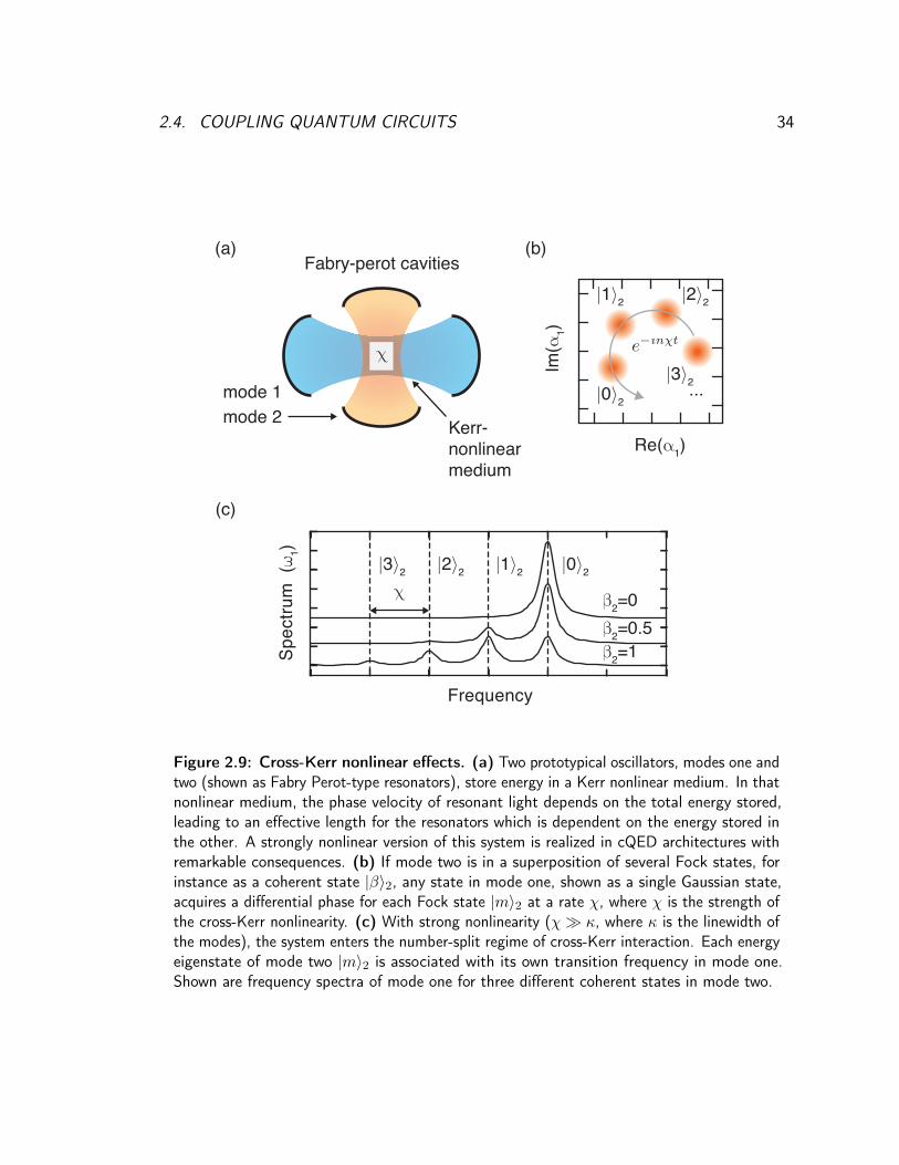
2.4. COUPLING QUANTUM CIRCUITS 34
Frequency
Spec
trum
(ω
1)
Re(α1)
Im(α
1)
(c)
(a)
0〉2
3〉2
2〉21〉2
0〉2 ...
1〉22〉23〉2β2=0β2=0.5β2=1
(b)
mode 1mode 2
χ
Kerr-nonlinearmedium
Fabry-perot cavities
χ
Figure 2.9: Cross-Kerr nonlinear effects. (a) Two prototypical oscillators, modes one andtwo (shown as Fabry Perot-type resonators), store energy in a Kerr nonlinear medium. In thatnonlinear medium, the phase velocity of resonant light depends on the total energy stored,leading to an effective length for the resonators which is dependent on the energy stored inthe other. A strongly nonlinear version of this system is realized in cQED architectures withremarkable consequences. (b) If mode two is in a superposition of several Fock states, forinstance as a coherent state |β〉2, any state in mode one, shown as a single Gaussian state,acquires a differential phase for each Fock state |m〉2 at a rate χ, where χ is the strength ofthe cross-Kerr nonlinearity. (c) With strong nonlinearity (χ κ, where κ is the linewidth ofthe modes), the system enters the number-split regime of cross-Kerr interaction. Each energyeigenstate of mode two |m〉2 is associated with its own transition frequency in mode one.Shown are frequency spectra of mode one for three different coherent states in mode two.

2.4. COUPLING QUANTUM CIRCUITS 35
a Kerr term proportional to
Kk =EJϕ
4k
4(2.97)
This is a little strange. Our circuit under consideration began as a transmon sub-circuitcoupled to many LC oscillators, but somehow, we ended up with just a bunch of transmons!In retrospect, this might not be too surprising since a transmon, in our treatment, hasbeen a nonlinearly-shunted LC oscillator. Surely then, by introducing the same nonlinearityto the other LC oscillators, they might be expected to dress with the Josephson effect in asimilar manner.
At fourth order, we acquire a new type of Hamiltonian term as well that has interestingconsequences for our circuit. We now find terms in the expansion that are a cross-Kerrtype nonlinearity [62], as
Hint = −EJϕ2aϕ
2b a†ab†b. (2.98)
We define the cross-Kerr interaction strength as χab ≡ EJϕ2aϕ
2b . Note that χ is related to
the geometric mean of the two Kerr terms as
χab = 2√KaKb. (2.99)
This makes intuitive sense since this nonlinear interaction is set by how hybridized eachmode is to the single Josephson junction in the problem. That same hybridization alsosets Kn.
For two modes with a large detuning, χab is the dominant coupling term. This regimeis known as the dispersive regime of cQED [62], a Hamiltonian that has also obtained withCQED [11]. Now, if mode a is excited, for example in the Fock state |1〉a, our dispersiveHamiltonian indicates that the frequency of mode b will shift downward by exactly χ, since〈a†a〉 = 1 for Equation 2.98. A more interesting behavior is achieved whenever one ofthe modes is in a superposition of Fock states. Then, an entangling interaction occurs[11], whereby a superposition of Fock states in one mode forces the other mode to be in aconditional superposition of many frequencies, as we will discuss in detail in Chapter 3. Inthe next section, we show how this conditional frequency shift can be used to devise aQND measurement of the qubit state.

2.5. DETECTING THE STATE OF A TRANSMON 36
2.5 Detecting the state of a transmon
It might be interesting to probe a transmon directly with a Vector Network Analyzer(VNA), for instance, measuring the atom in reflection, similar to the scheme of Hoi etal. [63]. In this case, when the VNA (at weak probe powers) sweeps through a transitionfrequency of an occupied level of our transmon, a single probe photon (at most) will beexchanged with the transmon. Detecting a missing photon (absorption) or an extra photon(emission) would inform us of the former state of the transmon. However, practically thisis a demanding requirement. Additionally, the real impedance of the VNA would introduceunnecessary dissipation to the transmon, as we will discuss later in Section 4.2.1.
Instead, we will couple our simple transmon circuit to a filter element, an ancillary LCoscillator [54, 55], and probe the response of the oscillator to infer information about thestate of the transmon [14, 64]. To detect the state of mode a, we need to determine modeb’s frequency with sufficient precision to determine whether it is ωb or ωb − χ. There aresome nice properties of this proposal. First, if we can drive mode b with many photons,our frequency detector does not need to be sensitive to fluorescence-like signal levels asconsidered before. Also, this detection can be QND to good approximation [59, 60]. Thisis opposed to schemes which rely on absorption or fluorescence, which detect a change ofstate. Finally, if the readout mode is more strongly coupled to the detection apparatus, itwill filter real impedance of the detector from the transmon atom, extending the possiblelifetimes in the transmon mode [56].
Now, however, our readout mode has acquired some transmon-like behavior as shown inthe previous section. However, for a carefully designed circuit, we can largely ignore theseeffects, and pretend that our filter retains its linearity. This is a reasonable approximationfor the readout mode whenever
Kb|〈b†b〉|2 1/Texp (2.100)
where Texp is the timescale for the experiment. Essentially, for a weak nonlinearity, thenumber-state dependent phase accumulation by the Kerr effect may take more time toacquire than we are sensitive to.
To use the conditional frequency shift of the readout mode (δω = χ) as a detectionmechanism, sufficient frequency precision is required. Therefore, the measurement time
2.5. DETECTING THE STATE OF A TRANSMON 37
will be on the order of Texp ≈ 1/χ. By Equation 2.100, we then require that
χab Kb〈b†b〉. (2.101)
Therefore, we must design circuits that have a large χab/Kb ratio. Using Equation 2.99,we find that these requirements can be distilled to working with a transmon having highanharmonicity, such that
Ka Kb|〈b†b〉|2. (2.102)
Essentially, the above constraint is the extent to which we can assign the label ‘transmon’to one mode and ‘resonator’ to the other. In practice, this inequality is easily satisfiedbecause usually only the transmon mode is galvanically connected to the junction. Forinstance, we will study a sample in detail in Chapter 6 that fulfills this requirement up to〈b†b〉 ≈ 500.
To show how the simplest readout schemes operate, consider our coupled Hamiltonian,with the transmon truncated at its lowest two levels (Eq. 2.73), and ignoring the resonator’snonlinearity [54]. In the interaction picture, the Hamiltonian is given by
Hdisp =χab2b†bσz. (2.103)
This expression is equivalent to the dispersive limit of the Jaynes-Cummings model forCQED [11], albeit derived with a different set of systems, assumptions and approximations.
A typical technique for measuring the frequency of a resonator is to measure thereflection coefficient of signals from the device [14, 64]. That coefficient is given by
r =∆b − ıκ/2∆b + ıκ/2
(2.104)
where ∆b is the detuning between the probe and the resonator. For a probe tone tunedhalfway between the response of mode b to the transmon (ωd = ωb − χ/2), r can berewritten to account for the state-dependent shift [14] as
r =χσz − ıκ/2χσz + ıκ/2
. (2.105)
If we define a the angle θ = κ/χ we can simplify the reflection as a rotation in the IQplane as
r = e−ıθσz . (2.106)

2.5. DETECTING THE STATE OF A TRANSMON 38
Re(α)Time
Sign
al
Im(α
)
(b) (c)
Frequency
Sign
al(a)
κ κ
χ
Figure 2.10: Reading out the state of a transmon. (a) The frequency of the readoutresonator depends strongly on the state of the transmon qubit. The frequency shift χ canbe much greater than the linewidth of the mode κ. To probe the state of the transmon, acommon technique is to drive halfway between these two frequencies (purple arrow). Then,the state of the transmon is encoded in the phase of the outgoing signal. (b) A readoutpulse builds up energy in the resonator that is leaked out to the measurement chain. For thereadout probe frequency shown in (a), the two states of the transmon yield identical ring-uptype envelopes. c) The amplitude and phase of these signals are digitized, via techniquesdescribed in a later chapter, and the measurement results are histogrammed. The relativecounts between the two distributions gives the probability the qubit was detected in theground or excited state (Pg and Pe).

2.5. DETECTING THE STATE OF A TRANSMON 39
For a coherent input state, in the absence of the resonator’s Kerr nonlinearity, thisphase angle is independent of the displacement size [14]. Therefore, phase contrast,our measurement signal, will increase with larger displacements. We can quantify theinformation contained in the reflected signal as the orthogonality of the resultant coherentstates. If the two states of the transmon (|0〉a, |1〉a, or equivalently |g〉, |e〉) are mappedonto a phase difference θ, the coherent states can be detected in unique states to theextent that
〈αe+ıθ|αe−ıθ〉 = 0 (2.107)
We give the practical details of this detection scheme later in Section 5.2.4.
2.5.1 Selection rules for many-wave mixing
We conclude our study of the simplest coupled-oscillator Josephson circuits with somestriking effects that can be observed by stimulating otherwise negligible processes in thecircuit with pumps.
We rely on the commutativity of our different modes in order to go into a co-rotating,co-displaced frame [34], such that all modes can be driven by some field, transforming ouroperators as
An → An + ξn. (2.108)
Our total Hamiltonian recovers a generalized form of Equation 2.62. A remarkable set ofinteractions can be driven between the elements of our many-transmon artificial molecule.
If we take the simplest experiment, driving a single mode off resonantly, the χ interactionat fourth order approximation ends up every mode an AC Stark shift [34]. Driving then-th mode shifts the m-th mode by an amount
∆m = −χnm|ξn|2. (2.109)
Also, similar the multi-photon transitions of a single transmon, strong pumps can drivemulti-photon processes in the coupled circuit [34]. For example, a pump on mode n at afrequency ωd = ½(ωm − ωn) would make stationary any terms in the Hamiltonian of theform
Hswap = −χnm[ξ2An
†Am + (ξ∗)2AnAm†]
(2.110)
We see that this Hamiltonian term can be used to swap single photons between modes, suchas the transmon and resonator, by exchanging energy with two probe photons (four-wave

2.5. DETECTING THE STATE OF A TRANSMON 40
Figure 2.11: Josephson junction as a scattering site. Many Hamiltonian terms are dis-carded by energy conservation considerations during the polynomial treatment of a Josephsonjunction’s cosine potential. However, in the presence of drives, these otherwise neglectedterms can dominant the evolution of the system. Pumping a single junction at multiplefrequencies can lead to a versatile set of mode conversions via many-wave mixing.
mixing). For a cold resonator with fast decay constant, this technique can be used forto reset another mode [34]. Or, driven between two coherent modes, this pump can beused for SWAP-based quantum logic [65]. Interestingly, these SWAP interactions typicallyrequire resonant operation [65] (and thus frequency tunability), which can complicatecircuit implementations. Here, we get that physics ‘for free’ from the quartic term of ourcosine expansion.
As another example, take the pump frequency ωd = (2ωm − ωn). Energy-conservingterms now include
Hswap = −χnm[ξ(An†)2
Am + ξ∗(An)2
Am†]
(2.111)
Just by changing the frequency of the pump, we have altered the four wave mixing suchthat now one photon from mode m is converted to two photons in mode n and vice-versa,by exchanging energy with a single pump photon. This parametric process was used inLeghtas et al. [34] to drive an oscillator directly to a cat state.
There is an infinite number of interesting processes we can stimulate with many-wavemixing [37]. The recipe is simple enough to be extended to even higher order terms beyondquartic. These experiments will push the cosine expansion in new ways. Single Josephsonjunction circuits seem to be an endless playing field for fundamental quantum optics.
Before diving into the physical implementation of these systems, the next chapterexplores the consequences of quantum information in resonators. Future chapters will

2.5. DETECTING THE STATE OF A TRANSMON 41
discuss the specifics of transmon-resonator design Chapter 4 as well as techniques for theirfabrication and measurement Chapter 5. Then we will combine these ideas to describe anovel type of quantum memory that has state-of-the-art coherence for cQED, in Chapter 6.

CHAPTER 3
Quantum information in harmonic oscillators
Harmonic oscillators are very simplest quantum mechanical objects, as we saw inChapter 2. However, the infinite Hilbert space of a harmonic oscillator can be
leveraged for powerful applications in quantum information processing [66, and referencestherein]. We begin this chapter by motivating oscillator-based quantum informationschemes with an example from modern classical communication techniques [67]. We thenturn our attention to quantum states in oscillators, describing how to characterize suchstates [11] and how to create them using the ideas from Chapter 2 [68, 69]. Finally, wereview recent progress toward one exciting application for qubit-coupled resonators, theso-called cat-codes for quantum error correction. [70].
Many of the concepts throughout this chapter are general to the control and measure-ment of oscillators. Whenever possible, we show how the dispersive interaction describedin the previous chapter enables the particular process at hand. Many other qubit-resonatorinteractions are possible and have their own set of advantages and disadvantages [26, andreferences therein]. In particular, resonant SWAP gates between qubits and resonators,in which single excitations are swapped or manipulated, have been used to demonstratea remarkable set of experiments [71]. Side-band pulses can also be used to create non-classical qubit-resonator states [72–74] and mediate quantum information storage in anoscillator [75].
42

3.1. PHOTONS CARRYING CLASSICAL BITS 43
3.1 Photons carrying classical bits
This chapter is influenced by the modern signal processing techniques of digital phase-shift-keying (PSK) [67], which is reviewed here to highlight its similarities to quantumschemes, as pointed out in [68].
Fiber optic cables are ideal transmission channels for long distance communicationbecause they are low-distortion and low-loss. However, installing fiber optics cables andrepeaters is an expensive endeavor. Techniques that maximize the capacity of each signalchannel are crucial to enabling modern high speed communication at large scale. PSKrelies on the fact that telecommunications signals are carried by waves. By comparing thephase-difference (φ0) between an incoming signal and a reference clock, we can determineφ0 to some, potentially high, precision. That precision sets the number of points in phasespace that can be used as classical bits.
An additional benefit of phase encoding is that it is naturally robust against smallamounts of signal loss, as compared to amplitude encoding which is maximally sensitive toloss. As long as the signal remains above the noise floor such that φ0 can be determinedto the requisite precision, PSK is robust against dissipation. This idea is analogous andimportant for quantum mechanical versions of PSK, as we will see later in this chapter.
As shown in Figure 3.1, quadrature-PSK encoding (QPSK) is one example of suchan encoding scheme. The sender of a QPSK message chooses one of four offset-phasesφ0 ∈ [±π/4,±3π/4], such that the sent message is
s(t) = V0 cos(ωt+ φ0). (3.1)
The receiver mixes down the message against two orthogonal basis functions (sine andcosine) to recover the phase symbol
Im =
∫ Ts
0
cos(ωt)× V0 cos(ωt+ φ0)dt (3.2a)
Qm =
∫ Ts
0
sin(ωt)× V0 cos(ωt+ φ0)dt (3.2b)
It simplifies demodulation to choose the integration time to be a full period Ts = 2π/ω,though this is not a requirement of QPSK. Then,
(Im, Qm) ∈ V0Ts
2√
2(−1, 1), (1, 1), (1,−1), (−1,−1) (3.3)

3.1. PHOTONS CARRYING CLASSICAL BITS 44
LORF
Im
Qm
0.0 0.2 0.4 0.6 0.8 1.0Time0.0
0.2
0.4
0.6
0.8
1.0
-10
±101
-10
±101
Im
Qm
+
+
Im
Qm
-
+
-
-
+
-
(i) (ii)
(iii) (iv)
(a) (b)
Time
(c)
Im
Qm
(i)
(ii)(iii)
(iv)
Figure 3.1: Phase shift-keying (PSK) of classical signals. (a) In transmit mode, a localoscillator (LO) is mixed with two sinusoidal voltages Im and Qm that carry a four-bit messageencoded in the phase of these oscillating voltages for a predetermined amount of time. Themodulated output signal (RF) is sent across a channel to the receive party. The receiverworks in reverse. There, the RF chain carries a modulated input signal that is down-convertedto phase-information containing components (Im,Qm) by a local oscillator. (b) Four bitsare encoded in a single time channel by setting the initial phase of independent sinusoidalfunctions as φ0 ∈ 0, 2π, which relies on the orthogonality of the cosine and sine functions.(c) Each transmitted symbol will be modulated or demodulated to a location on the IQ planethat falls on the PSK constellation shown. For signal strengths greater than the noise of thesystem, many bits can be encoded in each symbol, provided that the constellation points donot overlap to the precision of a given error threshold.

3.2. STATE TOMOGRAPHY OF AN OSCILLATOR 45
where we enumerated the results for phases increasing from φ0 = −3π/4. Noise sets thelimit on the density of phase-space at our disposal. A common PSK constellation caninclude between 16 and 32 bins for φ0. Therefore, in one integration window, the symbolcontains up to 32 bits of information.
A subtle issue with PSK is that the rapid switching of the phases between symbols cancause issues if any of the components, such as optical repeaters and amplifiers, have finitebandwidth or linearity [67]. To combat these problems, only certain transitions betweensymbols are allowed and information becomes encoded in the pattern of symbols, ratherthan single symbols themselves. Indeed, this idea indeed has also been considered forfinite-nonlinearity PSK analogues in the quantum domain.
If we had quantum control over a PSK-type communication channel, it is not too hardto imagine one could encode a similar number of quantum bits of information for eachsymbol. The sender only needs a component which can phase-shift a coherent state into asuperposition, i.e. modulate a signal to phase multiple phases at once. Remarkably, suchcontrol has already been demonstrated. At the conclusion of this chapter, we will reviewan experiment that has achieved the quantum version of QPSK, and we examine someimportant applications of such an encoding.
First however, we need a more sophisticated suite of tools to describe quantum statesin continuous variables systems.
3.2 State tomography of an oscillator
For an infinite-level system, full state tomography [39] is impossible [21]. In practice, wewill truncate any oscillator under study at some N -th level [11]. We require that anypopulation in higher levels is negligible to sufficiently describe the state. To see why this isjustified, consider a coherent state of amplitude |β〉 , the probability of finding populationat a high Fock state (N |β|2) is given by Equation 2.21, which falls off precipitately.For instance, for the coherent state |β|2 = 9, if we truncate our tomography at N = 18,the total population in higher states is only 0.5%.
Further, coherent states are an overcomplete decomposition of the oscillator’s Hilbertspace [21]. Zurek showed that for state tomography, the minimum grid-size for a givenprecision is related to the size of the allowed N -th level truncation of the Hilbert space [76].Essentially, any features in state tomography will be required to have slower variation thansome δα [76]. Therefore, most tomography schemes proceed by gridding the Hilbert space

3.2. STATE TOMOGRAPHY OF AN OSCILLATOR 46
into a series of IQ-blocks of size δα× δα that are accessed with a displaced measurementoperator [11], examples of which we will describe starting in Section 3.2.2.
3.2.1 Fock state distribution
The simplest, but potentially incomplete, tomography that can be conducted on the stateof a resonator is obtained by measuring the probability distribution of Fock states, each Pn,up to some truncation. Such a tomography scheme is useful for detecting non-Gaussianstatistics in a resonator state [62] and for calibrating control drives [38] as we discuss inSection 6.2.1.
In the strong dispersive regime of cQED, spectroscopy on the qubit reveals the Pndistribution automatically [62]. Essentially, because the qubit acquires a large frequencyshift for each resonator Fock state χ γ2 (where γ2 is the full qubit linewidth), therelative area of the n-th number-state resolved transition line (the ‘nth number-peak’)gives Pn. Assuming a sufficiently weak drive on the qubit and assuming that the linewidthof the qubit is γ2 ≈ 1/T1, the spectrum of the qubit is given by [64]
S[ω] =C
2π
∑n
(Pnγ2
(12γ2)2 + (ω − ω0 − nχ)2
)(3.4)
where C is a scaling term to account for the readout efficiency and ω0 is the frequency of thetransmon conditioned on zero photons in the resonator, i.e. the transition |g, 0〉 → |e, 0〉.We use this technique to confirm the preparation of non-classical states in Chapter 6.
We caution the reader that pulsed spectroscopy is recommended for this tomographytechnique. The alternative, which would seek to quantify the statistics of a steady-stateresonator drive by measuring the spectroscopy signal of a transmon in parallel, leads toseveral complications [64]. First, the presence the resonator drive will Stark shift thetransmon spectrum (Section 2.3.4), shifting the observed resonator and qubit spectra as
∆stark,r = −Kr|ξr|2
∆stark,q = −χ|ξr|2(3.5)
where |ξr|2 is the resonator drive intensity, Kr is the Kerr of the resonator, χ is thedispersive coupling strength between the qubit and resonator. Importantly, this is adifferent term in the Hamiltonian than χa†ab†b that provides number splitting (i.e. isquantized). As soon as the drive, ξ is turned off (as for pulsed spectroscopy) this term

3.2. STATE TOMOGRAPHY OF AN OSCILLATOR 47
will disappear. Furthermore, as described in Section 2.5.1, drive terms in the Hamiltoniancan stimulate previously discarded conversion terms. This can yield additional features inspectroscopy, making interpretation difficult. Yet, as long as the experiment is conductedcarefully and pulsed, the protocol for determining χ in spectroscopy is straightforward.
By measuring the transmon’s spectrum then, we can determine whether the distributionof Pn is Poissonian (coherent states), super-Poissonian (e.g. thermal states), or sub-Poissonian (e.g. Fock states) [62]. Examples of ideal distributions are given in Figure 3.2.Since a single Fock state carries no phase information, a Pn distribution is sufficient tocompletely characterize such states. However, for states that lack rotational symmetry inthe IQ plane, additional information is needed to characterize the system.
3.2.2 Husimi Q functions
The Husimi Q function [77] is a quasiprobability distribution that quantifies the oscillator’spopulation at a given point in IQ grid (R(α), I(α)) as the overlap between the inputoscillator state and a coherent state of amplitude |α〉. More precisely, for the input state|ψ〉, the Q function at grid-point α can be written as
Q(α) ≡ 1
π|〈α|ψ〉|2 (3.6)
To see how this quantity is extracted experimentally, we can rearrange the above as [21]
Q(α) =1
π|〈0|D†(α)|ψ〉|2 =
1
π|〈0|D(−α)|ψ〉|2. (3.7)
We see that, by symmetry, the task of measuring the overlap of |ψ〉 with a finite amplitudecoherent state reduces to measuring the overlap of |ψ′〉 = D(−α)|ψ〉 with the zeroth Fockstate (P0), which we saw in the previous subsection was possible. Examples of Husimi Qfunctions are given in Figure 3.3.
Rather than spectroscopy, we can measure P0 more efficiently [38] by driving thetransmon with a number-selective π pulse that is narrow frequency (FWHM χ) andresonant on the |g, 0〉 → |e, 0〉 transition, followed by a measurement of the qubit state.This technique can be quantum non-demolition (QND) [78, 79], meaning that regardlessof the input state, a measurement of the transmon in the excited state |e, 0〉 will heraldthe preparation of a zeroth Fock state. Measuring the resulting transmon state in |g〉 will

3.2. STATE TOMOGRAPHY OF AN OSCILLATOR 48
Spec
trosc
opy
0.00.20.40.60.81.0
Prob
abilit
y
Spec
trosc
opy
0.00.20.40.60.81.0
Prob
abilit
y
-4 -3 -2 -1 0 1Detuning
Spec
trosc
opy
0123456Fock state number
0.00.20.40.60.81.0
Prob
abilit
y
(Δ/χ)
(a)
(b)
(c)
Figure 3.2: Quantifying the statistics of a resonator state. (left) Examples aregiven of various qubit spectra under different preparations of resonator states. (right) Thecorresponding probability distribution of resonator Fock states (Pn) that would be inferredfrom the associated qubit spectrum. (a) The resonator is in a coherent state of β = 1.0and obeys Poissonian number statistics. (b) The resonator is in a single Fock state |3〉 anddisplays sub-Poissonain number statistics (the variance in n of zero is less than the meanvalue of three). (c) The resonator is either in a superposition of |0〉 and |3〉 or in a statisticalmixture of the two states. A simple probability distribution Pn is not sufficient to distinguishthese two cases.

3.2. STATE TOMOGRAPHY OF AN OSCILLATOR 49
project the state into a vacuum subtracted version of the input state [79], i.e.
|ψ〉final = N (|ψ〉input − C0|0〉) (3.8)
where C0 is the initial state’s amplitude in |0〉. The N accounts for the renormalization ofthe state to maintain
∑∞n=1 |Cn|2 = 1, where the new amplitudes are scaled to account
for the missing population the vacuum.In general, more information can be extracted about the oscillator state if the qubit is
found to be in |g〉 since some other Cm remains nonzero with statistics that are directlyrelated to the input state [79]. However, for tomography protocols which only seek tomeasure the state of an oscillator, it is more accurate to instead recycle the system, waitingfor it to return to equilibrium before preparing another input state and measuring it. Thetrade off for discarding additional information is that the resulting tomography can beinterpreted without concern for uncontrolled measurement backaction, such as qubit decayduring measurement [80].
The Husimi Q function can also be generalized to extract a more sensitive set ofinformation about an oscillator input state [11]. Instead of probing just the overlap with acoherent state (equivalently a displaced |0〉 Fock state), one can measure the overlap withany displaced Fock state as
Qn(α) =1
π|〈n|D(−α)|ψ〉|2 (3.9)
It follows that Qm of the m-th Fock state is identical to the Gaussian profile of the Q0 ofthe vacuum.
Any one of the generalized Qn functions is a complete representation of the inputstate’s density matrix [21]. However, some quantum features tend to be suppressed inthis type of tomography. Figure 3.4 shows that a way of recovering that sensitivity is tocombine many Qn distributions into a single observable across an oscillator’s Hilbert space,such as the parity operator [38, 71], defined as
P ≡ eıπn. (3.10)
Measuring the expectation of some operator 〈O〉 at a location in IQ space α is equivalentto
〈O〉α = Tr(D†(α)ρD(α)O
), (3.11)

3.2. STATE TOMOGRAPHY OF AN OSCILLATOR 50
−2 0 2
−202
−2 0 2 −2 0 20
1⟨2 Q0 ⟩
Re(α)
Im(α
)
δαj
δαi
cavity
qubit
Q-functionprepare
(a) (b)
Re(α)Re(α)Re(α)
Im(α
)
(c)(i) (ii) (iii) π
Figure 3.3: Husimi Q distribution of resonator states. (a) Experimental sequence toperform Husimi Q tomography on a resonator state. The tomography is performed after somearbitrary preparation step, which leaves the qubit unentangled with the resonator. To measurethe Q function at a displacement α, a displacement of D†(α) = D(−α) is used to bringthat region of the state to the origin. Then, a number selective qubit rotation is performedthat flips the qubit to the excited state only if zero photons are present. Measurements arerepeated to acquire the quasiprobability distribution across many values of the displacedmode. (b) Graphical representation of Q function measurement. The IQ plane of theresonator is broken up into grids, where each block represents a displacement value used inthe experimental sequence. (c) Examples of Q functions. The Husimi Q representation ofthe resonator states previously considered in Figure 3.2 can reveal more information. (i) Acoherent state of β = 1ı is distinguishable from β = −1ı. (ii) The Q function of the |3〉Fock state has no further information since the state has complete phase uncertainty. (iii)The superposition of |0〉 and |3〉 is distinguished from a statistical mixture by the existenceof a rotational asymmetry in the state’s Q function.

3.2. STATE TOMOGRAPHY OF AN OSCILLATOR 51
which can be expanded as
〈O〉α =∑n
〈n|(D†(α)ρD(α)O
)|n〉. (3.12)
Fock states are eigenstates of the parity operator: P |n〉 = (−1)n|n〉. So the aboveexpansion reduces [21] to
〈P 〉α =∑n
(−1)n〈n|(D†(α)ρD(α)
)|n〉. (3.13)
Rearranging the density matrix gives a simple form for this expectation value as
〈P 〉α =∑n
(−1)n|〈n|D†(α)|ψ〉|2 (3.14)
which we recognize as a sum over Qn as defined in Equation 3.9. We finally have that
〈P 〉α = π∑n
(−1)nQn(α) (3.15)
Again, we truncate this series at some N above which QN tends to zero at small displace-ments (|α|2 . N). By measuring many generalized Qn functions, we are able to extractdirectly a useful quantity to describe our state. In fact this particular observable is directlyrelated to another type of tomography, the Wigner function. In the next subsection, wemeet the Wigner function and a more direct measurement technique for 〈P 〉α.
3.2.3 Wigner tomography
The Wigner function [21] is a quasiprobability distribution that is formally defined as
W (α) =2
π〈P 〉α. (3.16)
The function takes values in the range of W (α) ∈ [−2/π, 2/π], and it is normalized suchthat ∫
W (α)dα2 = π. (3.17)

3.2. STATE TOMOGRAPHY OF AN OSCILLATOR 52
Q0 Q1 Q2 Q3 ⟨2 Q ⟩π nQ4
(a)
(b)
- -+ + ...
...
waitpulse pulset =
(i) (ii) (iii) (iv)
Figure 3.4: Two techniques for measuring parity. (a) Parity can be determined byan alternating sum of generalized Qn functions [21]. This is a graphical representation ofEquation 3.15 for an even superposition of coherent states |ψ〉 = |β〉+ |−β〉. The first panel,which is Q0, does not contain noticeable information about the superposition. However, thehigher even functions Q2, Q4 have weight at the center, whereas the odd functions Q1, Q3
have zeros at the center, indicating that the state has a strong positive parity at the origin.This shows explicitly what is meant by parity having more quantum phase sensitivity. (b) Analternative method for measuring parity in a ‘single-shot’ is shown [68, 81]. An initial π/2pulse puts the qubit on the equator of the Bloch sphere. If the resonator state has manyphotons (colored Bloch vectors), the qubit will dephase by the dispersive interaction. At arevival time t = π/χ, the Bloch vectors associated with odd photon numbers (blue) will haveacquired a π phase shift, while the evens (red) will have acquired 2πn of phase. At this time,a final π/2 maps the parity information onto the qubit state. A measurement of the qubitstate thus makes a projective parity measurement of the resonator state.

3.2. STATE TOMOGRAPHY OF AN OSCILLATOR 53
With these conventions, a number of useful relations hold. Most importantly, the densitymatrix of a given state is given by an integral over the Wigner function [21] as
ρ =2
π
∫W (α)D(α)PD†(α)dα2 (3.18)
Thus by probing the Wigner function experimentally, we gain direct insight into the densitymatrix of the oscillator’s state. It can further be shown that the Q0 function is related tothe Wigner function as
Q0(α) =2
π
∫W (β)e−2|α−β|2dβ2. (3.19)
This convolution is simply a Gaussian filter over W . Therefore, we expect the Wignerfunction is more sensitive to detecting structure in the IQ plane. Indeed, the Wignerfunction has an additional, useful detection property for quantum states: no oscillatorclassical state can have negativity in its Wigner function [82]. It has also been demonstratedtheoretically that a negative Wigner function can be a resource for a quantum informationprocessing speed-up [83, 84].
In order to assemble a state’s Wigner function, we could in principle measure each Qn
and compute Equation 3.15. However, this requires tens of Pn’s to be measured at eachpoint on the IQ grid which is burdensome. Instead, the dispersive interaction gives us theopportunity to make projective measurements of P directly [81].
Figure 3.5 shows how a projective parity measurement is conducted with the dispersiveHamiltonian, used for Rydberg atoms with CQED [81] and for transmon atoms with cQED[68]. The goal of the protocol is to flip the qubit if and only if the resonator is in aneven (or odd) parity state. The measurement begins with an unselective π/2 pulse on thequbit (FWHM Nχ) that brings the qubit’s Bloch vector to the equator. As we sawearlier, if many Fock states in the resonator are populated, the qubit no longer has a welldefined frequency. Consequently, each Bloch vector associated with a different Fock statewill acquire phase a different rate, φ = nχt [85]. A second π/2 pulse will become moreineffective as these states spread out, appearing as a Gaussian T2 decay. Yet, this systemrevives in a very special way after a characteristic time Tp = π/χ [68]. Examining thetotal state at t = Tp, we have
|ψ(t = Tp)〉 =∑n
Cn(|g, n〉+ eıπn|e, n〉
). (3.20)

3.2. STATE TOMOGRAPHY OF AN OSCILLATOR 54
We see that at the time Tp, each odd Fock state acquires a π phase shift, while eacheven Fock state returns to the initial point on the Bloch equator (2π phase). Therefore,a second π/2 pulse, along the same axis will bring the even subspace to the excitedstate, while the odd subspace is rotated to the ground state. To summarize, this protocoltransforms the system as∑
n
Cn|g, n〉 ⇒∑n∈odds
Cn|g, n〉+∑
n∈evens
Cn|e, n〉. (3.21)
Now, the probability of detecting the qubit in the excited state (Pe) is directly related tothe probability that the resonator had an even parity. So the expectation of the parityoperator is simply now
〈P 〉 ∝ Pe − Pg. (3.22)
The lack of equality in the above expression arises from our inability to conduct thisparity mapping and qubit readout with unit efficiency. However, we can calibrate outthese inefficiencies by taking tomography of a known state, such as the vacuum state,and normalizing our tomography to the visibility of this signal [68]. While this lacks therobustness required for claiming violating quantum measurement inequalities [79], it isoften useful to separate out state preparation fidelity from tomographic errors.
As shown in Figure 3.5, the full protocol for performing Wigner tomography in thedispersive regime of cQED is a combination of parity measurements and displacements onthe resonator. It is illustrative to compare the distributions across Figure 3.2, Figure 3.3,and Figure 3.5 to see how the same resonator state can be described in many ways.
3.2.4 Flying state tomography
An important class of techniques have been developed to perform tomography on photonicstates that are not confined to resonators but rather traveling down a measurement chain[86, 87]. Once a state is ‘flying’, the experimentalist may lack many of the tools wepreviously took for granted, including coherent control over the mode (access to D(α)), aphoton-number resolving detector (access to Pn), or a direct parity meter (access to 〈P 〉).Instead, the complete density matrix of a propagating field can be reconstructed using atechnique known as optical homodyne tomography.
Homodyne detection is implemented by combining a field under study (Es) with astrong local oscillator (ELOe
−ıωt+ıφ) at a beam splitter [87], which produces two outputs

3.2. STATE TOMOGRAPHY OF AN OSCILLATOR 55
cavity
qubit
wigner-tomographyprepare
(a)
Re(α)Re(α)Re(α)
Im(α
)
(b)(i) (ii) (iii)
=
−2 0 2
−202
−2 0 2 −2 0 2-1
0
+1⟨P⟩
Figure 3.5: Wigner tomography in cQED. (a) Experimental sequence to perform Wignertomography on a resonator state. As in the sequence for Husimi-Q functions, we begin withsome arbitrary state in the resonator that is unentangled with the qubit. Like Q-functions,Wigner tomography is measured across different displacement values α. A displacement ofD†(α) = D(−α) brings a section of the Hilbert space interest to the origin. Then, twounselective qubit π/2 pulses, separated by a delay time t = π/χ, maps the parity of theresonator to the qubit state. Measurements are repeated to acquire the quasiprobabilitydistribution across many values of the displaced mode. (b) Examples of Wigner functions.The Wigner representation of the resonator states previously considered in Figure 3.2 andFigure 3.3. The Wigner function can reveal more information than either of these techniques.(i) A coherent state of β = 1ı has a smaller Gaussian width in a Wigner function as comparedto the Husimi Q distribution, making Wigner a more sensitive technique for resolving smalldifferences in amplitude or phase. (ii) The Wigner function of the |3〉 Fock state again hasno further information compared to Pn or the Q function. However, an important feature ofnegativity in the Wigner function clearly distinguishes this state from a classical one. (iii)The superposition of |0〉 and |3〉 is distinguished from a statistical mixture by the existence ofa rotational asymmetry and distinct regions of negativity in the quasiprobability distribution.
3.2. STATE TOMOGRAPHY OF AN OSCILLATOR 56
that, for balanced detection (using a 50/50 beam splitter), are given by
E± =1√2
(ELOe−ıωt+ıφ ± Es). (3.23)
In optical detection schemes, these arms are measured by sensitive square-law detectors.If the field under study has quadratures that oscillate at ω, the time dependence isaveraged out from the signals. Subtracting the outputs from the two detectors gives theexperimentalist access to
|E−|2 − |E+|2 = 2ELOEs(φ). (3.24)
Varying the phase of the LO traces out the statistics of the field under study across the IQplane [87]. Alternatively, performing a heterodyne measurement (ωs 6= ωLO) reveals bothquadratures in parallel, at the cost of a quanta of added noise.
To be more precise, we can define a set of scaled, rotated quadratures [87], as
xφ =1√
2nLO
(X cosφ+ Y sinφ
)yφ =
1√2nLO
(−X sinφ+ Y cosφ
) (3.25)
where X, Y are defined as in Equation 2.16. Our homodyne protocol consists of a seriesof measurements to obtain a distribution at each φ that is a histogram of amplitudesPφ(Xφ). Because the probability distribution of any observable is given by an integral overthe state’s Wigner function, we have that
Pφ(xφ) =
∫ ∞−∞
W (−xφ cosφ+ yφ, xφ sinφ+ yφ cosφ)dyφ. (3.26)
The Wigner function can be obtained by inverting the above integral with a Radon transform[88]. Treating noise, detector inefficiencies, and finite numbers of measurements can alsobe treated by approximate inversion techniques [87] such as the maximum likelihoodmethod [89].
For detectors that are linear, as opposed to square-law, a similar set techniques areavailable [90]. If we count the number of integrated measurements that fall in an IQ-bin,e.g. [R(αi + ε), I(αi + ε)], we have essentially measured the overlap of the signal understudy with a coherent state with amplitude αi. By the definition of the Husimi Q function

3.2. STATE TOMOGRAPHY OF AN OSCILLATOR 57
(Eq. 3.7), we recognize that this measurement probes Q0 for a traveling wave. Next, weconsider an important type of linear detector-based flying state tomography, the dispersivereadout scheme of cQED [64].
Dispersive readout as tomography
Performing a measurement of the qubit state in the dispersive regime of cQED can beaccomplished by interrogating a strongly-coupled, harmonic readout mode. As describedin Section 2.5, we analyze the output field of the readout mode in order to discriminatethe qubit state-dependent phase imparted during the interaction time. In the followingdiscussion, we relate this concept to the types of tomography considered here.
We can write the input-output relations [91] for a resonator populated with some stateA(t) as
aout(t) =√κA(t)− ain(t), (3.27)
where ain and aout are input and output modes, respectively (for details, see for in-stance [90]). We integrate that signal with a Heaviside step windowed function f(t) =√κe−κt/2Θ(t) to obtain our signal mode [92] as
a =
∫f(t)aout(t)dt. (3.28)
Our linear amplification chain provides gain (G) to our signal and introduces a noise modeh that acts as a noise term so that our final complex amplitude signal operator is given by
S =√G(a+ h) (3.29)
The resulting histograms are a Husimi Q function on S which are scaled from the originalsignal quasiprobability distribution as Qout(S) [90], so that
Qout(√Gα) =
1
GQin(α) (3.30)
The added noise from the vacuum mode can be shown to enter as a convolution, whichfor the Gaussian states typically used for readout, only results in in a broadening of theGaussian distribution, as a thermal field. For signal chains that contain low-noise HEMTamplifiers, the full added thermal field corresponds to ∼ 20K, while for chains that includenear-quantum limited parametric amplifiers, it can be below 1K [93].

3.3. DISPERSIVE CONTROL 58
To perform a dispersive measurements on a transmon qubit, we require that the twomeasurement distributions Qout(Sg) and Qout(Se) are well separated. As the resonator isdisplaced to some coherent state |β〉, we rely on the dispersive interaction to impart arelative phase shift conditional on the state of the qubit [64]. The resu broadened Gaussianhistograms as δφ ∼ χτ where τ is some the effective signal decay time on the order ofn/κ. Two coherent states of equal amplitude, but rotated by δφ have the separation
|〈βeıδφ|β〉|2 = e−|β−βeıδφ|2 = e−2|β|2 sin2(φ/2) (3.31)
Importantly, for strong projective measurements, we see that for a given phase shift, alarger amplitude coherent tone will be a more effective measurement. However, if thesystem has nonlinearity in the readout chain, either in the readout resonator or in thesaturation of the amplifier, there will be some optimal strength that is difficult to predicta priori.
3.3 Dispersive control
Now that we have several methods for quantifying non-classical fields within a resonator,we turn our attention to creating such states. We review a few recent ideas for creatingtarget states in a harmonic oscillator by leveraging the dispersive interaction. First, wepresent a method for mapping the superposition state of a qubit onto the phase of adisplaced oscillator state, the so-called QCMap gate [94]. QCMap is a powerful techniqueto create a superposition of many Fock states in a single gate application [68]. Next, weshow how individual Fock states can be manipulated with a Selective-on Number ArbitraryPhase (SNAP) gate [69, 95]. SNAP can be used to build arbitrary states in a stepwisefashion, similar to the SWAP gates discussed in Section 2.5.1.
3.3.1 QCMap gate
Essentially, the QCMap works in the reverse of the parity measurement we presented inSection 3.2.3. Rather than map the parity of the resonator onto the state of the qubit fordetection, we map the state of the qubit onto the parity of a displaced resonator state [94].In particular, QCMap can be used to put qubit states of the form |ψ〉q = Cg|g〉+Ce|e〉 ontosuperpositions of coherent states |ψ〉r = Cg|β〉+Ce|−β〉. If the qubit had been in a equalsuperposition, Cg = ±Ce, the resonator is taken to a parity eigenstate, having a either

3.3. DISPERSIVE CONTROL 59
all even photons (+) or odd photons (−), while preserving Poissonian statistics centeredaround |β|2. Such a state is commonly referred to as a cat state [11], since the phase ofa large coherent state approaches a classical variable. Indeed, the size of the resultingsuperposition is arbitrary in the gate’s functionality and is only set by system imperfections.Therefore, QCMap is an interesting testbed for quantum to classical transitions [68], inaddition to being a potentially useful quantum memory operation [70], as we consider atthe conclusion of this chapter.
To perform a QCMap operation, we initialize the system with the qubit in |ψ〉q andthe resonator in a coherent state |β〉, such that the total system state vector is
|ψ〉 = (Cg|g〉+ Ce|e〉)⊗ |β〉 (3.32)
The dispersive interaction will evolve the ground and excited states of the combined systemwith a frequency difference χ that we can absorb into the definition of the coherent state
|ψ(t)〉 = Cg|g, β〉+ Ce|e, βeıχt〉. (3.33)
After a time Tp = π/χ, again the dispersive Hamiltonian will yield a π phase shift betweenthe two subspaces, leaving
|ψ(t = Tp)〉 = Cg|g, β〉+ Ce|e,−β〉. (3.34)
At this point, the system is in a Schrödinger cat state [11], since measuring the two-levelstate of the qubit would provide complete information over the nearly-classical coherentstate phase variable. In analogy to the famous Gedanken experiment, the qubit acts as aspontaneously decaying atom which determines the fate of our feline-like phase.
We complete the QCMap gate by removing the entanglement between qubit andresonator. This is done in two steps. First, a non-selective displacement D(β) is performedon the resonator to yield
|ψ〉 = Cg|g, 2β〉+ Ce|e, 0〉. (3.35)
Then, a qubit rotation that is selective on the zeroth Fock state, as in Section 3.2.2, takes|e, 0〉 → |g, 0〉, leaving
|ψ〉 = |g〉 ⊗ (Cg|2β〉+ eıφCe|0〉), (3.36)
where the phase term accounts for a Berry phase that can be acquired depending on therelative trajectory of the qubit rotation. The resonator is left in a state that is commonly

3.3. DISPERSIVE CONTROL 60
referred to as an amplitude-cat [11] for obvious reasons. A final displacement D(−β)
restores the symmetry to the system, and, fixing the Berry phase at φ = 0, gives
|ψ〉 = |g〉 ⊗ (Cg|β〉+ Ce| − β〉). (3.37)
In a pioneering experiment [68], this procedure was confirmed to take an arbitrary qubitstate to an arbitrary resonator state of the above form. Additionally, extensions of thesimple QCMap gate can be constructed for evolution times t = Tp/m, which can be usedto create m-legged cat states. We discuss the connection between these states and errorcorrection in the final section of this chapter.
3.3.2 SNAP gate
The Selective-on Number Arbitrary Phase (SNAP) gate allows for universal quantumcontrol over a harmonic oscillator by making active use of the dispersive interaction[69, 95]. A SNAP gate is constructed by driving the qubit on a closed trajectory on itsBloch sphere. The backaction of the enclosed area imparts a Barry phase on the system|g〉 → eıφ|g〉 [96]. The key observation for SNAP is that the qubit only undergoes suchan evolution conditionally on a Fock state in the resonator, taking |g,m〉 → eıφ|g,m〉.This phase accumulation is differential between the selected Fock state and the rest of theresonator’s state vector [95]. Classical drives on the resonator can be used to interferethese differential phases. By interleaving displacements with SNAP rotations then, onecan build up complex quantum sates in the resonator. For instance, a single SNAP gateand two displacements on the resonator is sufficient to generate an N = 1 Fock statein the resonator [69]. We present this example in detail to get an understanding of theSNAP framework.
An intuition for the protocol can be gained by considering a qubit trajectory that isalong a single axis, e.g. a 2π-pulse along the qubit’s x-axis. This great-circle trajectoryaccumulates a π phase shift on the state [96]. Therefore, if the pulse is selective onthe mth Fock state, the amplitude Cm will acquire a sign flip [69]. An additional smalldisplacement can be thought of as a mixing of neighboring Fock states, which might nowbe out of phase and therefore interfere in a nontrivial way. In practice, the size of thedisplacement operations are numerically optimized to maximize the fidelity of the finalstate [95].

3.3. DISPERSIVE CONTROL 61
We show how these operations can be combined explicitly for the creation of a Fockstate. First, a displacement of D(1.14) on the resonator generates a coherent state in theresonator that has
|ψ〉r =0.522|0〉+ 0.595|1〉+ 0.480|2〉
+ 0.316|3〉+ 0.180|4〉+O(0.1)[≥ |5〉].(3.38)
The qubit rotation imparts a Barry phase of φ = 2π on the |0〉 state, leaving the resonatorin
|ψ〉r =− 0.522|0〉+ 0.595|1〉+ 0.480|2〉
+ 0.316|3〉+ 0.180|4〉+O(0.1)[≥ |5〉].(3.39)
A final displacement operation D(−0.56) takes the resonator to
|ψ〉r =− 0.048|0〉+ 0.990|1〉+ 0.003|2〉
+ 0.133|3〉+ 0.002|4〉+O(0.01)[≥ |5〉].(3.40)
Indeed, a perfect set of operations can prepare the N = 1 Fock state with P1 = 0.98
[95]. This preparation fidelity can be further improved by additional SNAP operations.Unfortunately, as we discuss in Chapter 6, system imperfections can limit the resultingstate fidelity before the fundamental limits of these operator-level considerations. Itis worth remarking too that the nontrivial statistics of the small remaining populationP3
∑n6=1 Pn arises from the interference effects inherent in the SNAP gate.
For a full proof of the universality of this protocol, we refer the reader to [95]. However,we present a simpler argument here based on continuous variables quantum computation[97]. Because it is straightforward to impart an infinitesimal phase on each number state,we can scale the imparted phases such that they are polynomial in n. We can thusgenerate an artificial nth-order nonlinearity. This was actually demonstrated with SNAPexperimentally for a fourth-order nonlinearity in [69]. Because such a nonlinearity causesincreasing orders of operators by commutation [97], e.g.[
K(X2 + Y 2)2, X]
=1
2
(X2Y + Y X2 − 2Y 3
), (3.41)
we simply need to alternate SNAP gates will classical drives to synthesize an arbitrarilyhigh order Hamiltonian [97].
So far, we have seen how to characterize and control the Hilbert space of our linear,

3.4. DECOHERENCE IN AN OSCILLATOR 62
cavity
qubit
(a)
2π0
Re(α)−2 0 2
Re(α)
⟨P⟩
−2 0 2
-1
0
+1Im(α
)
−202
β1 β2
SNAP
Im(α
)
−202
(b)
(i)
(i) (ii) (iii)
(ii) (iii)
Figure 3.6: Creating nonclassical states via SNAP. (a) An experimental sequence forarbitrary state preparation in a resonator via SNAP. This technique interleaves classicaldisplacements on the resonator with number-selective Berry phases on the qubit. Becausethe Berry phase is number-selective, resonator Fock states can be interfered by applicationsof the displacement operator, which can leave the resonator in a highly nonclassical state.(b) Step-by-step creation of a Fock state via two displacements and a single qubit rotation.A coherent state is generated from driving the resonator with classical drives. By rotatingthe phase on the vacuum state by π, the resonator is left in a displaced |1〉 Fock state. Afinal displacement returns the Fock state to the origin.
continuous variables resonator. To explore the utility of such a resource, in Section 3.5,we review a proposal for quantum error correction for oscillators [70] and experimentalprogress towards its realization. First though, we put on solid footing why such schemesare necessary.
3.4 Decoherence in an oscillator
Quantum states in resonators are always eventually spoiled by interactions with theenvironment. For instance, resonator photons can be exchanged with a thermal bath,or the phase of a quantum superposition can be randomized by unitary evolution. Thecost of relying on the large Hilbert space of an oscillator is that the sensitivity to theseinteractions increases rapidly for macroscopic superposition states [11].
In this section, the effect of energy exchange between a general resonator density matrix

3.4. DECOHERENCE IN AN OSCILLATOR 63
and a thermal bath is considered, treating the resonator as an open quantum system.Phase noise is treated in a similar manner, introducing a phase scattering process with thebath to compute its effects.
Previously, we evoked terms like an energy decay rate κ without a rigorous quantummechanical description. In order to recover that description, we rely on the Lindblad formof the quantum master equation (QME) [35]. This allows us to solve for the evolution ofthe density matrix of the resonator given some spurious process. The model assumes theexistence of a bath system whose degrees of freedom are sufficiently numerous that theevolution of the bath is not greatly affected by its interaction with the resonator (Markovapproximation) [35]. Under this condition, the generic Lindblad form of the QME givesthe evolution of the resonator density matrix as
dρ
dt=−ı~
[H, ρ
]+∑k 6=0
(LkρL
†k −
1
2L†kLkρ−
1
2ρL†kLk
), (3.42)
where Lk are jump operators which describe the interaction with the bath. Specificexamples of these decoherence mechanisms are given next.
3.4.1 Energy decay
The basic form of energy damping is an exchange interaction between the resonator and abath [35] as
Hint =∑k
Ω∗kc†ka+ Ωkcka
†, (3.43)
where the rates Ωk determine the amount energy exchange. We can define a set of jumpoperators L↑, L↓ that account for the resonator gaining or losing a photon from a bath[35]. These are
L↑ =√κ↑a
† (3.44a)
L↓ =√κ↓a. (3.44b)
If the bath reservoir is a temperature T , Boltzmann’s Law requires that these rates arerelated by a Boltzmann factor
κ↑κ↓
= e−~ω0/kbT (3.45)

3.4. DECOHERENCE IN AN OSCILLATOR 64
where ω0 is the frequency of the resonator and kb is Boltzmann’s constant. By Planck’sLaw, the thermal state should have an average number of photons in each mode as
nth =1
e~ω0/kbT − 1=
1
κ↓/κ↑ − 1. (3.46)
Rearranging this expression gives
κ↓ = (1 + nth)κ (3.47a)
κ↑ = nthκ, (3.47b)
where a single decay rate κ is used to normalize the up and down rates. We recognize thenκ terms to account for the hopping of a (thermally) displaced field.
We can write down a Lindblad equation to describe this evolution of the resonatorunder this interaction [35] as
dρ
dt=− ı
~[~ω0a
†a, ρ]
− (1 + nth)κ
2
(a†aρ+ ρa†a− 2aρa†
)− nthκ
2
(aa†ρ+ ρaa† − 2a†ρa
).
(3.48)
To go further, we can consider the populations of individual Fock states, essentiallysandwiching the above expression as
dPndt
= 〈n|dρdt|n〉, (3.49)
which gives a rate equation for Pn [35] as
dPndt
= Γ↑Pn+1(t) + Γ↓Pn−1(t)−[(
n
n+ 1
)Γ↑ +
(n+ 1
n
)Γ↓
]Pn(t). (3.50)
The rates are calculated to be
Γ↑ = (1 + nth)(n+ 1)κ (3.51a)
Γ↓ = nthnκ. (3.51b)
In equilibrium, we require that the probabilities are stationary (dPn/dt ≡ 0), which

3.4. DECOHERENCE IN AN OSCILLATOR 65
immediately gives us a condition on the probabilities as a function of the thermal field
PnPn−1
=nth
1 + nth(3.52)
which is again a simple Boltzmann factor as one would naively expect.Importantly though, Equation 3.50 allows us to consider states out of equilibrium [35].
If some state in the resonator has a mean number of photons n 6= nth, the state will evolvetowards equilibrium as
dn
dt=∑k
kdPkdt
(t) = −(n− nth)κ. (3.53)
This is a quite remarkable result, meaning that any excited state of the resonator willhave an expected energy that decays as an exponential [20]
E(t) = ~ω0n(t) = ~ω0((n0 − nth)e−κt + nth), (3.54)
where n0 is the initial mean field in the state.The exponential shape of Equation 3.54 is reminiscent of two-level system T1 decays
with T1 = 1/κ [39]. In fact, we can immediately conclude that if the resonator has n0 = 1,regardless of the actual distribution of Pn, the averaged energy decay will be equivalent toa T1 experiment, provided that n(t) is the extracted quantity experimentally.
In general, the off diagonal components of ρ, which contain the coherences betweenFock states, decay in a highly nontrivial manner under amplitude damping [11]. As anexample, we consider the effect of energy decay on an equal superposition cat-state of theform |ψ〉 = N (|β〉+ | − β〉), the initial density matrix is
ρ(t = 0) =1
2[|β〉〈β|+ | − β〉〈−β|+ |β〉〈−β|+ | − β〉〈β|] (3.55)
Here, the cross terms (ρ[β,−β] and ρ[−β,β]) contain the coherences between the two coherentstates. Under the action of Equation 3.61, the coherent state amplitudes acquire a trivialdecay term [11]
|β(t)〉 = |βe−κt/2〉 ≡ |β〉. (3.56)
However, the coherence between the coherent states decays much more rapidly [11], as
ρ[β,−β](t) = e−2n(1−exp(−κt))ρ[β,−β](0). (3.57)

3.4. DECOHERENCE IN AN OSCILLATOR 66
Therefore, the true ‘T2’ of the state, i.e. the rate of phase information loss, is for shorttimes (κt 1) given by
T2 ≈1
2nκ. (3.58)
For macroscopic superpositions, n 1. Therefore, T2 T1, even though energy decay isthe only decoherence mechanism present!
3.4.2 Phase noise
The Lindblad formalism is applicable to phase noise as well [35]. In this case, the interactionwith the bath does not exchange resonator photons between the modes (as in the case ofenergy decay). Instead, the effect is a modification of the resonator’s resonant frequency asa scattering process, in which a bath quantum is created or destroyed while the resonatorphoton number is conserved,
Hint =∑k
Ω∗kc†a†a+ Ωkca
†a (3.59)
where the rates Ωk determine the amount of frequency perturbation by the reservoir. Wecan define a pair of jump operators that account for emitting and absorbing bath quantain order to acquire exchange energy, but at zero temperature, we are left with a singleoperator
Lφ =√
2Γφa†a. (3.60a)
(3.60b)
Here, the QME is given by [35]
dρ
dt=− ı
~[~ω0a
†a, ρ]
− Γφ(ρ(a†a)2 + (a†a)2ρ− 2a†aρa†a
).
(3.61)
We are particularly interested in the evolution of off-diagonal elements of the form
dρnmdt
=(−ıω0(n−m)− Γφ(n−m)2
)ρnm. (3.62)
Again, we find an exponential damping of our solution. Here,
ρnm(t) = e−ıω0(n−m)te−Γφ(n−m)2t (3.63)

3.5. QUANTUM ERROR CORRECTION ON CAT-CODES 67
We find that random modulations of the resonator frequency washes out coherence rapidlyfor distant coherences (|n−m| 1). Therefore, macroscopic superpositions will be highlysusceptible to dephasing. We can define a pure dephasing time Tφ = 1/Γφ, such that thetotal ‘T2’ of the resonator is then
1
T2
=1
2T1
+1
Tφ(3.64)
However, we caution the reader that the simple decay of two level systems is only applicableto resonators when we truncate the Hilbert space of the resonator to the same number oflevels as we will do in Chapter 6.
3.5 Quantum error correction on cat-codes
All quantum error correction schemes rely on storing quantum information across redundantdegrees of freedom and accessing joint properties of the system to correct errors [98, e.g.].It was recognized by Leghtas et al. [99] that because the Hilbert space of a resonator isinfinite, a single resonator could provide a resource-efficient subspace for storing redundantquantum information. In this section, we present a code that corrects for photon-loss incat states of a cQED resonator [70, 99]. These so-called cat-codes are the basis for alogical quantum computing scheme.
3.5.1 Cyclic photon-loss
Photon-loss is a dominant error channel in circuits [9, 100]. However, coherent statesare eigenstates of the annihilation operator [21]. If a photon is lost from a resonator in acoherent state, nothing happens. Instead, the state deterministically loses amplitude atrate κ/2, which can be corrected after some time dt with a displacement of amplitudeε = κdt/2. Certainly, for a classical bit of information, this is an appealing property.
It turns out that superpositions of coherent states have an interesting consequence forphoton-loss mechanisms too [99]. Consider the even parity eigenstate
|ψ〉 =1√2
(|β〉+ | − β〉) . (3.65)

3.5. QUANTUM ERROR CORRECTION ON CAT-CODES 68
Losing a photon in this state results in a phase flip,
a|ψ〉 =1√2
(|β〉 − | − β〉) . (3.66)
This phase flip takes us to the odd parity subspace. Parity measurements therefore, canact as a photon-loss error detector, without collapsing the state since |ψ〉 remains alwaysin a parity eigenstate [99]. Remarkably, this error tracking scheme has been experimentallydemonstrated in cQED [80]. However, the two-legged cat [11] can only encode a classicalbit of information (whether the parity is +1 or -1). To encode a quantum bit, each paritysubspace needs to contain an entire logical Bloch sphere [99].
One basis that can encode superpositions within a parity subspace are four-legged cats.Two pairs of orthogonal coherent states form a PSK-like constellation to provides logicalstates |0〉L and |1〉L as
|0〉L = N (|β〉+ | − β〉)
|1〉L = N (|ıβ〉+ | − ıβ〉) ,(3.67)
where N ≈ 1/√
2 since the states that form the basis are only approximately orthogonal.Now, a full quantum bit of information can be encoded in the state
|ψ〉L = C0|0〉L + C1|1〉L. (3.68)
This logical state is a four-legged cat, with phases and weights of each leg determining theprojected vector on the logical Bloch sphere [70]. Because our logical states are chosen inthe even parity subspace, all logical states have only even Fock weights [11], as
|ψ〉L =∑
n∈evens
Cn|n〉 (3.69)
Therefore the loss of a single photon will leave us in an odd parity basis. It is convenientto define logical error states [70] as
|0〉L = N (|β〉 − | − β〉)
|1〉L = N (|ıβ〉 − | − ıβ〉) .(3.70)
Detecting any of these error states will indicate that an error has occurred in the memory.To see how errors can be decoded, consider the action of the annihilation operator

3.5. QUANTUM ERROR CORRECTION ON CAT-CODES 69
−2 0 2
−2 0 2
−2 0 2
encoding
error
-
error
0〉L
1〉L
-
Re(α)
−202
Im(α
)
−202
Im(α
)−2
02
Im(α
)
−202
Im(α
)
(a) (b)
Re(α)
Re(α)
−202
Im(α
)
−202
Im(α
)
Figure 3.7: Cat-code logical qubit encoding. (a) The cardinal points on a logical Blochsphere are taken to be the even superposition of real valued coherent states | ± beta〉 andimaginary valued coherent states |± ıbeta〉, as defined in Equation 3.70. The Wigner functionof the logical states |0〉L (blue star) and |1〉L are shown for |β| = 3. (b) The effect ofrepeated photon loss events on an encoded qubit state. At the origin, we see that everyphoton loss event flips the parity of the state at the origin. After one loss, the negative parityhere indicates an error state. However, a second photon loss even leads to an undetectederror, since the state is back in the logical basis but at a new point on the logical Blochsphere.

3.5. QUANTUM ERROR CORRECTION ON CAT-CODES 70
on the logical qubit state. We define a counter state |ψ(k)〉L in order to keep track ofsuccessive photon loss events:
|ψ(k)〉L ≡ (a)k|ψ〉L. (3.71)
Remembering that for coherent states a|α〉 = α|α〉, we encounter a series of phase flipsfor the logical qubit
|ψ(0)〉L = C0|0〉L + C1|1〉L (3.72a)
|ψ(1)〉L = C0|0〉L + ıC1|1〉L (3.72b)
|ψ(2)〉L = C0|0〉L − C1|1〉L (3.72c)
|ψ(3)〉L = C0|0〉L − ıC1|1〉L (3.72d)
|ψ(4)〉L = C0|0〉L + C1|1〉L (3.72e)
We recognize immediately that |ψ(0)〉L = |ψ(4)〉L. Therefore, the photon-loss process iscyclic in our basis [70]. Consequently, our state is never destroyed by photon loss, thoughthe deterministic energy loss still occurs at rate κ. Techniques for overcoming energydecay are under active investigation [34]. These schemes rely on parametrically driving thesystem (Section 2.5.1) to ‘re-pump’ the energy back into the resonator deterministically.
Major milestones still remain for the nascent cat-codes. Although encoding a qubitstate onto a four-legged cat has been achieved [68], universal control over a logicalcat-qubit, for instance using the techniques in [69], is an important next step for thescheme. Additionally, extending the QND error-tracking scheme [80] to a full quantumbit in a four-legged cat will be a significant accomplishment. Furthermore, building onthe parametric drives already demonstrated for cat-codes [34] to demonstrate four-photonprocesses will be essential for the long-term success of oscillator-based QEC schemes.Finally, putting all of these pieces together, and showing overall gains in qubit performance,will be an incredible triumph.

CHAPTER 4
Photon boxes for cQED
Microwave resonators are an enabling technology in circuit QED. On their own, res-onators can serve as a test bed for studying material losses [101–104]. The lessons
gained from these measurements guide the development of cQED devices [105, 106].Coupled to superconducting qubits, low-loss resonators can act as quantum memories[52, 75, 107] or as buses for exchanging quantum information between qubits [57, 58].Resonators are also implemented to enable high fidelity measurements of qubit states [64]and to protect superconducting qubits from radiative losses [56].
This thesis is primarily concerned with one of these applications in particular, thequantum memory performance of a resonator. Therefore, we begin this chapter bypresenting a generalized framework for to describe how loss mechanisms affect resonators.With that context, we present the design and development of a suite of low-loss microwaveresonators and discuss the challenges and opportunities of a number of resonator geometries.This chapter culminates in the discovery of a viable technique for achieving state-of-the-artquantum memory performance for a superconducting-qubit-coupled device [52].
4.1 Quantizing a distributed mode
In earlier chapters, our circuits were compiled from discrete components such as inductorsand capacitors. We showed how such elements could lead to a quantized Hamiltonian
71

4.1. QUANTIZING A DISTRIBUTED MODE 72
which governed their quantum behavior. However, such lumped-element components donot exist in reality [108]. ‘Inductors’ and ‘capacitors’ are only approximate reactances,appropriate whenever the size of the component is much less than a wavelength. Inpractice, all circuit elements have some complex impedance that is neither completelycapacitive nor inductive. (nor even purely reactive for that matter). Further, the conceptof electromagnetic resonance is much more general than parallel or series circuits. Wewill see in this chapter that even with the same frequency and impedance, two microwaveoscillators can have very different physical properties, influencing their utility for cQED.
We are left with the need to generalize our Hamiltonian description from before. Whilea careful treatment is possible for any specific arrangement of metal and dielectric, we usetwo observations to simplify our work here, which are derived explicitly for a transmissionline in [14]. The first observation is that our electromagnetic mode should be well describedby a wave velocity νp = 1/
√`c, where ` and c are the inductance and capacitance per
unit length along some propagation axis (usually taken as z). Then, our circuit has welldefined flux and charge that oscillate at frequency ω as
Φ(x, t) = Φ(x, y)ej(ωt+βz) (4.1a)
Q(x, t) = Q(x, y)ej(ωt+βz), (4.1b)
where β = ω/νp is the propagation constant. The second observation that allows us towrite down the quantum mechanical description of such a system is the treatment ofboundary conditions [14]. Each resonator has a particular set of boundary conditions thatforces these wave equations to a set of discrete eigenmodes. Otherwise, the system wouldlack a meaningful, discrete resonance.
These distinct eigenmodes form a complete, orthogonal set of functions for flux andcharge in a closed geometry. A given distribution of electromagnetic energy can be writtenas a sum over these modes [14], such that
Φ(x, t) =∑n
CnΦn(x, y)ej(ωnt+βnz) (4.2a)
Q(x, t) =∑n
CnQn(x, y)ej(ωnt+βnz). (4.2b)
The boundary conditions and geometry of the resonator determine the frequency andspatial distribution of each eigenmode. We have a Hamiltonian for this generalized photon

4.1. QUANTIZING A DISTRIBUTED MODE 73
Figure 4.1: Black box quantization of a distributed mode. The LC oscillator circuits inChapter 2 are useful toy models that capture the physics of QED. In reality however, only theJosephson element can usually be treated as a lumped element. Distributed resonators canhave complicated mode structures, but once the eigenmodes of the linear system are known,we recover the equations of motion that would otherwise describe simple LC elements.
box asH = ~
∑n
ωna†nan, (4.3)
where each eigenmode has a distinct, commuting set of creation and annihilation operators.We can also generalize a circuit’s coupling to a lumped-element Josephson junction in
this language [109]. The linear part of the Josephson inductance may add another set ofeigenmodes to the system and perturb the existing ones, but we can account for this usingsimilar techniques as before [10]. We just need to re-diagonalize the modes. After thelinear system has been solved, we only need to know the location of the junction (x = xJ)to find the flux across the junction (i.e. the difference in flux at +ε), as
ΦJ =∑n
Cn
(Φn(xJ)− Φn(xJ + ε)
). (4.4)
It is this quantity that we use the for nonlinear part of the Hamiltonian (Eq. 2.45) thatgives us the rich physics we saw in the previous chapter. We see in later chapters explicitlyhow this term is calculated by full 3D simulations.

4.2. QUALITY FACTORS AND PARTICIPATION RATIOS 74
4.2 Quality factors and participation ratios
The quality factor of a resonator (Q) sets the ultimate limit for the resonator’s performanceas a quantum memory or bus. The quality factor is defined as
Q ≡ ωTotal energy stored
Total power dissipated= ωT1, (4.5)
where T1 is the energy decay time and is inversely related to the energy decay rate(T1 = 1/κ). Therefore, the ultimate quantum coherence that a resonator can posses isT2 = 2T1 = 2Q/ω. If a full circuit model is available, the quality factor can be calculatedby
Q =1
Z0ReY∣∣ω=ω0
, (4.6)
where Z0 is the characteristic impedance of the resonator (defined in Eq. 2.92).As shown in Figure 4.2, many sources of loss can contribute to a total quality factor.
The power dissipated in each of these loss mechanisms combines to make the the totalpower dissipated in the circuit equal to
Γtot =∑n
Γn, (4.7)
where each loss mechanism consumes power at rate Γn. Because the average total energystored in the resonator is a single quantity, we can write the quality factor as
1
Q=
1
ωEtot
∑n
Γn. (4.8)
A more convenient way to express the phenomenology of many sources of loss adding tothe total quality factor is to work in unitless quality factors defined as Qn = ωEtot/Γn, sothat the total quality factor can be expressed [110, e.g.] as
1
Q=∑n
1
Qn
. (4.9)
Note that Qn is represents net result of source of loss, combining both the lossiness of thesource and the sensitivity of the resonator to the loss mechanism. Changing geometrieswhile holding all of the materials properties constant will change Qn. Clearly, there is a need

4.2. QUALITY FACTORS AND PARTICIPATION RATIOS 75
...
Γ1 Γ2 Γ3
Γtot Γii
Figure 4.2: General loss mechanisms for a resonator. For a physical circuit, many lossmechanisms can contribute to the damping of energy in the system. The dissipation of eachof these elements adds to the total dissipation rate of the circuit. We can make progress inunderstanding a given total dissipation rate through experiments which selectively probe onesuch mechanism, such as conductor loss.
to express the sensitivity of a given resonator to a certain loss mechanism independentlyof the lossiness of the given mechanism.
This notion is already common for cavity resonators limited by conductor loss, wherea geometrical factor G is expressed in Ohms such that the observed quality factors areQ ≈ G/R [111], where R is the sheet resistance of the conductor used to fabricatethe resonator. For typical waveguide cavity geometries and frequencies, G ≈ 100 Ω suchthat typical room temperature conductors, e.g. copper with R ≈ 0.1 Ω/, gives roomtemperature quality factors of Q ≈ 1000. Designs with higher G achieve a higher Q for agiven metal. We generalize this notion to generic loss mechanisms next, as participationratios.
Participation ratios are a useful framework for quantifying loss in any device [112]. Theidea is to use straightforward accounting to interpret decay rates in a way that educatesa circuit designer about the losses in the system. These ratios can lead to surprisingconclusions about what limits a given performance [105, 106]. Comparing many variationsof one main geometry can test scaling hypotheses about certain loss mechanisms [104].In addition, comparing results from two entirely different geometries can inform a circuitdesigner about different types of loss present in both.
To accomplish this accounting, we simply re-express Qn to tease apart the geometry

4.2. QUALITY FACTORS AND PARTICIPATION RATIOS 76
dependence from the loss tangent of a mechanism, as a participation ratio
pn =Energy stored in mechanism
Total energy stored. (4.10)
Now, if the loss mechanism has a loss tangent tan δn, then
Qn =1
pn tan δn=qnpn. (4.11)
If the resonator stores all of its energy in a single degree of freedom its participation ratiois unity, px = 1, which implies that Q = qx. The key to designing a low-loss circuit is toknow what systems have high qn and store as much of the energy there as possible. Insubsection 4.2.3, we will see how G is explicitly connected to one of these ratios.
Let us look at a few classic loss mechanisms for a superconducting microwave resonator,using the language of participation ratios.
4.2.1 External loss
All resonators share a loss mechanism that is a direct consequence of coupling signalsinto and out-of such circuits [111]. If a circuit is coupled to a port, the real part of theport’s admittance will damp the mode to some degree. In fact, it is a common techniqueto actually over-couple a cQED resonator for readout purposes. Here, we show how thisarises for a simple toy model.
In Figure 4.3, an LC oscillator is capacitively coupled to a 50Ω load, which can be anaccess channel for drives or a path for signal to leak into the measurement chain. FollowingSchuster [62], the coupling capacitor transforms the real impedance of the load, which wecan recast as a parallel admittance as
Yext =1
R + 1/jωCext=
jωCext1 + jωCextR
. (4.12)
For weak coupling (ωCext R), Yext can be approximated as
Yext ≈ jωCext + ω2C2extR. (4.13)
The total admittance of the circuit is then
Ytot =1
jωL+ jωCtot + ω2C2
extR, (4.14)

4.2. QUALITY FACTORS AND PARTICIPATION RATIOS 77
Yext
(a) (b)C L Cext
Rinput/output
C L
Figure 4.3: Treating external dissipation. (a)All systems which are probed by an externalport are damped in the process. We introduce the toy model of an LC oscillator capacitivelycoupled to a 50Ω load to capture this effect. (b) In order to solve for the induced dissipationrate on the resonator, we recast the series coupling impedance to a parallel admittance,whose real part enters the calculation for Qtot as shown in this section.
where Ctot = C + Cc. To use Equation 4.6, we need the characteristic impedance
Z0 ≡ ωImY ′∣∣ω=ω0
=
√L
Ctot, (4.15)
since ω0 = 1/√LCtot. Then, we are ready to express a quality factor for the circuit
Qext ≈1
ω20C
2extZ0R
. (4.16)
When coupling to distributed modes, the same idea from this toy model holds. Introducinga real impedance to the circuit for control or readout purposes will be associated withsome external dissipation.
4.2.2 Dielectric loss
On resonance, a circuit stores an equal part of its energy in the mode’s electric andmagnetic fields [111]. Let us first quantify loss mechanisms which dissipate energy in theelectrical quadrature in the form of lossy dielectrics. A good room temperature PCB has adielectric loss of tan δ ≈ 2× 10⁻³ [113], while crystalline sapphire might have loss lowerthan tan δ . 1× 10⁻⁶ [114, 115].
There are two main channels for dielectric loss in a cQED experiment. First, energyis stored in the substrate that holds the artificial atom itself [115]. In addition, electrical

4.2. QUALITY FACTORS AND PARTICIPATION RATIOS 78
energy is stored at the surface of the superconducting metals, e.g. an oxide layer ALOx
and at the surface of the substrate [105, 106]. Both of these electrical surfaces can belossy.
These mechanisms are well described by participation ratios, albeit at very differentscales. We compute the dielectric participation ratio as
pdiel =
∫diel ε|E|
2dV∫tot ε|E|2dV
(4.17)
where the numerator integrates over the dielectric of interest, while the denominatoraccounts for all of the electrical energy stored in the device. Bulk dielectric participationratios tend to be in the range of pdiel ≈ 0.01− 1, as we will enumerate in later sectionsfor various geometries. Surface dielectrics, on the other hand, tend to have smallerparticipation by virtue of their significantly smaller physical volume.
It is often to useful to compute a simplified integral for surface participation. At asuperconducting surface, the tangential component of the electric field must go to zero(so that no voltage builds up on the conducting surface). Therefore, we only need toconsider the behavior of the perpendicular electric field at these interfaces. To calculatethe electric field inside of the surface layer (Esurf), we rely on the continuity of the D-fieldto find Esurf = Evol(εvol/εsurf), where Evol is the electric field in the vacuum. We canapproximate the integral in Equation 4.18 for this type of surface interface, considering athin oxide layer, as
pdiel ≈tox∫surf |Evol|2dA
εr,ox∫tot |Evol|2dV
(4.18)
where tox is the surface oxide thickness, εr,ox is the relative dielectric constant, and E0 isthe field strength in the vacuum. We point out that if the interface had been different,e.g. metal-dielectric-metal, the above expression would require modifying the ratio ofEsurf/Evol accordingly.
We can estimate the magnitude of the surface participation ratio for a generic resonatorgeometry by considering that the determining contribution is the ratio of volumes repre-sented by toxA and V , where A is the surface area of the resonator’s conductor, and V isthe total volume of the device. Therefore, a common rule-of-thumb estimation for pdiel ofsurface oxide is pdiel ∼ toxA/εr,oxV . For an infinite parallel plate capacitor, this expression
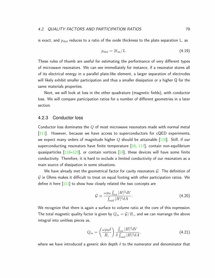
4.2. QUALITY FACTORS AND PARTICIPATION RATIOS 79
is exact, and pdiel reduces to a ratio of the oxide thickness to the plate separation L, as
pdiel = 2tox/L. (4.19)
These rules of thumb are useful for estimating the performance of very different typesof microwave resonators. We can see immediately for instance, if a resonator stores allof its electrical energy in a parallel plate-like element, a larger separation of electrodeswill likely exhibit smaller participation and thus a smaller dissipation or a higher Q for thesame materials properties.
Next, we will look at loss in the other quadrature (magnetic fields), with conductorloss. We will compare participation ratios for a number of different geometries in a latersection.
4.2.3 Conductor loss
Conductor loss dominates the Q of most microwave resonators made with normal metal[111]. However, because we have access to superconductors for cQED experiments,we expect many orders of magnitude higher Q should be attainable [116]. Still, if oursuperconducting resonators have finite temperature [18, 117], contain non-equilibriumquasiparticles [118–120], or contain vortices [18], these devices will have some finiteconductivity. Therefore, it is hard to exclude a limited conductivity of our resonators as amain source of dissipation in some situations.
We have already met the geometrical factor for cavity resonators G. The definition ofG in Ohms makes it difficult to treat on equal footing with other participation ratios. Wedefine it here [111] to show how closely related the two concepts are
G ≡ωµ0
∫tot |H|
2dV∫surf |H|2dA
. (4.20)
We recognize that there is again a surface to volume ratio at the core of this expression.The total magnetic quality factor is given by Qm = G/R, and we can rearrange the aboveintegral into unitless pieces as,
Qm =
(ωµ0δ
R
) ∫tot |H|
2dV
δ∫surf |H|2dA
, (4.21)
where we have introduced a generic skin depth δ to the numerator and denominator that

4.2. QUALITY FACTORS AND PARTICIPATION RATIOS 80
represents the exponential decay of magnetic field into our conductor. In the parenthesis,we have a term ωµ0δ which can be interpreted as a surface reactance XS [121], since µ0
has units of inductance per meter. Then, the quantity in the parenthesis is a unitless ratioof XS/R which we can understand as an effective conductor quality factor qcond for themetal [100]. For normal metals, qcond = 1 [111]. In fact, switching to a more conductivenormal metal increases Q by reducing the δ in the denominator of the integral-ratio. Thatunitless ratio of integrals is pcond, as
pcond =δ∫surf |H|
2dA∫tot |H|2dV
, (4.22)
which we will explore in detail next.The conductor participation ratio has a long history in superconducting circuits, where
it also known as the kinetic inductance fraction (α) [122]. For a superconducting resonator,the correct δ is the penetration depth λ [121]. Because this parameter defines a circuit’ssensitivity to conductor loss, it also describes the circuit’s sensitivity to quasiparticles.Circuits with large pmag are used as detectors for astronomy, called Microwave KineticInductance Detectors (MKID’s) [122], where quasiparticle signals are used to detect aphoton flux.
Unlike dielectric participation ratios, pcond can be revealed experimentally for a super-conductor through direct means [121, 122], as we describe in detail in Chapter 5.
4.2.4 Contact resistance
Any cQED experiment is assembled from parts that are individually fabricated, for instanceSMA connectors that route signals between devices and cabling [62]. The connectionsbetween components which carry RF energy can introduce dissipation in the form ofspurious contact resistance at seams [123]. Seam loss is especially important wheneverbolting two halves of a cavity together to form a high Q resonator [100, 124] or wheneverassembling and introducing wire bonds to planar circuitry [125].
Following Brecht et al. [123], we model this loss as a generic conductance G whoseloss-profile is constant as g∅ = G/L along a seam of length L. The conductance dG of asmall section dl along the seam is
dG = g∅dl. (4.23)

4.2. QUALITY FACTORS AND PARTICIPATION RATIOS 81
The incremental power dissipated by a small amount of current along dl by dG will be
dP =1
2
(dI)2
dG=
1
2
(J⊥dl)2
g∅dl=J2⊥dl
2g∅, (4.24)
where dI is the current flowing across dl, and the surface current J⊥ is given by a magneticfield tangential to the current H‖ as
J⊥ = n×H‖. (4.25)
Therefore, the total dissipated power can be written as
P∅ =
∫dP =
1
2g∅
∫H2‖dl. (4.26)
Then, the quality factor of the mode due to this loss mechanism [123] is
Q∅ =ωµ0
∫H2dV
P∅= ωµ0g∅
∫H2dV∫H2‖dl
=g∅y∅. (4.27)
The above expression has a very similar form as the participation ratios discussed earlier.However, allowing units in the dissipation term g∅, unlike tan δ for example, preventsus from having to make further assumptions about the dissipation. Additionally, we candefine an effective admittance per unit length for the seam as
y∅ ≡∫H2‖dl
ωµ0
∫H2dV
. (4.28)
The term y∅ acts like the participation ratio for seam loss, giving a quality factor that isinversely proportional to y∅ as
Q∅ =g∅y∅. (4.29)
We observe that locating cavity joints at regions of small magnetic field, or at least smallcurrent density across the seam (small y∅), is important for maximizing Q∅ and thus Qtot
[123].
4.2.5 Summary of loss mechanisms
The examples in this section have not exhausted all of the possible dissipation mechanisms incQED devices. However, participation-ratio accounting techniques are a general framework.

4.3. PLANAR RESONATORS 82
If a new loss mechanism is encountered, it can likely be described as an effective lossycapacitor (pdiel), lossy inductor (pcond), or discrete conductance element g∅.
In the remainder of this chapter, we present four types of resonator that have applicationsto cQED. For each resonator, we provide derivations and estimates for the participationratios studied here. In addition, we also explicitly state how Qext is calculated andunderstood for each device. Finally, we discuss how transmon-type qubits can be coupledto each type of photon box to realize cQED devices.
4.3 Planar resonators
Planar, thin-film resonators begin life as a bare dielectric wafer. Then, the conducting circuitis patterned on the wafer through either photolithography or electron-beam lithography.These steps are similar to the ones reviewed in a later chapter for transmon lithography.For now, let us consider the electrodynamics of one popular type of planar resonator, theCPW transmission line resonator [126, 127].
4.3.1 Resonant modes of a CPW
A transmission line is constructed from two conductors, where one acts as a ground planeand the other as a signal-carrying center-pin [111]. The impedance of the line Z0 isdetermined by the inductance and capacitance per unit length as
Z0 =
√`
c. (4.30)
Electromagnetic radiation traveling down such a transmission line a length z acquiresphase as ejβz. Upon encountering an impedance discontinuity (Z 6= Z0), the signal isreflected with a complex reflection coefficient [111]
V −
V +=Z − Z0
Z + Z0
. (4.31)
where V +, V − are the incoming, outgoing waves. If the discontinuity is an short circuit(Z = 0) or an open circuit (Z =∞) the magnitude of this reflection coefficient is unity,meaning that the boundary is equivalent to an infinitely sharp potential well.
Not surprisingly then, two such reflections (open-open, open-short, etc.) are sufficientto create a standing wave [62]. For the case of an open-open line, the fundamental

4.3. PLANAR RESONATORS 83
(a) (b)
ground plane
center trace
ground plane
CΣ pE
gw(i)
(ii)
Figure 4.4: Planar resonators and transmons. (a) Cartoon of planar device. (i) Sideview. Metal (silver), typically niobium or aluminum, is patterned on a substrate (green),typically silicon or sapphire. The impedance of resulting circuits is determined by the ratio ofthe width w of metal traces to the gap g separating the trace from the ground plane. Theimpact of lossy material (red outline) is also determined by the dimensions of the circuit. (ii)Top view. A gap in the center trace (yellow box) acts as a coupling capacitor and creates theconditions for resonance. The bend in the CPW line achieves a smaller physical package withnegligible effect in the microwave domain. A transmon (red) is located between the centertrace and ground plane. (b) Zoom of the transmon-resonator integration. The dynamicsare mediated by the dipole coupling of the transmon element (p) and the fields of the CPWmode (E). The nonlinearity of the Josephson junction is shunted by the capacitance of thetransmon (CΣ).
resonance has a wavelength λ0 = 2L, where L is the length of transmission line. If theboundary condition was instead open-short, the fundamental resonance occurs for λ0 = 4L.Most planar resonators are one of these types.
For CPW resonators, a transmission line is formed by a central conductor of width w,separated by a gap g from a ground plane [127]. These values are chosen to achieve acertain characteristic impedance for the transmission line, usually Z0 ≈ 50 Ω. Typical valuesfor CPW design parameters are w ∼ 10− 100µm and g ∼ 1− 50µm. State-of-the-artCPW resonators reach internal quality factors of Qint ∼ 106 [103].

4.3. PLANAR RESONATORS 84
4.3.2 Input-output coupling
We treated reflections from a resonator’s open boundary condition as an infinite potentialwell in the previous subsection to aide in our quantization of planar circuits. However, to getmicrowave signals into and out-of CPW resonators, the impedance only ever approximatesinfinite. A common technique is to implement a small break in the center conductor[62, 128], introducing a gap between the resonator and the signal carrying transmissionline. Then, the termination impedance is given by a coupling capacitance,
Zc = 1/jωCc. (4.32)
We see that as Cc is reduced to zero, Zc tends to infinity, and the reflection coefficientwill return to unity. A full circuit model can predict an external quality factor Qext fromthe dimensions of the discontinuity [62]. However, because the two-dimensional treatmentof planar circuits is an approximation, fringing fields may lead to spurious, unintended lossif not treated properly [128].
4.3.3 Planar transmons
Transmons on planar circuity tend to have dimensions that are much smaller than awavelength (50µm λ ∼ 5mm) [129]. Therefore, a lumped-element approximation iswell-suited to evaluate the Hamiltonian parameters, e.g. χij, Ki. As shown in Figure 4.4,a capacitance network is typically used to calculate parameters [62, op. cit. Section 3.3],such as the transmon anharmonicity
Kq ≈e2
2CΣ
, (4.33)
where CΣ is the capacitance of the total network given by
CΣ = Cg + C||, (4.34)
and Cg the gate capacitance is from the center trace to the ground plane across thetransmon and C|| is the capacitance directly between the two transmon antenna pads.Additionally, the self-capacitance of the resonator Cr must be known in order to properlynormalize the coupling strength.
The capacitance network can also be used to predict the magnitude of the cross-Kerr

4.3. PLANAR RESONATORS 85
coupling strength between qubit and resonator (χrq) and next order Hamiltonian terms[62, op. cit. Section 3.3]. For instance, the strength of the dispersive interaction is
χrq ≈g2ωq
4∆(∆−Kq), (4.35)
whereg ≡ e
CgCΣ
√ωr
2Cr. (4.36)
The two-dimensional circuit approximation allows even complicated, many-transmon circuitsto be designed. There has been a steady increase in the number of transmons on a planarcircuit [16, and references therein], with current state-of-the-art circuits having nineindividual transmon elements [46].
The performance of planar transmons has steadily improved too [16, and referencestherein]. Recent experiments have shown many transmon circuits where all of the transmonshad T1 & 20µs [46]. Continued development of materials and designs for these circuitspromises even more exciting physics results from this architecture.
4.3.4 Losses
Loss mechanisms in planar resonators and transmons have been the subject of manyexperimental investigations [103, 104, 130–133]. A common trend from these results isthat larger features yield lower loss devices until a radiation limit [134] is reached. Carefulparticipation ratio accounting allows different experimental groups to compare materialswith a common set of explicit assumptions about a given loss mechanism [105, 131]. Wegive such a table at the end of this chapter (Table 4.2).
To approximate participation ratios for planar circuits, we can apply our rule-of-thumbestimates for a CPW’s pdiel and pcond. Consider the case of surface dielectric loss at theinterface between the metal of the planar circuit and the vacuum between conductors. Wecan roughly approximate the capacitance of the CPW as a parallel plate capacitor. Then,for a CPW with gap size g (as Fig. 4.4), the interface would participate (Eq. 4.19) aspdiel ∼ 2tox/εrg, where tox = 3 nm, g = 10µm and εr = 10 [105], gives pdiel ≈ 3× 10⁻⁵.If instead, we consider the interface between the metal of the CPW and the substrate ofthe circuit, the boundary conditions give a factor of εr larger pdiel, indicating that thisinterface is particularly important for achieving high quality circuits.

4.4. RECTANGULAR CAVITY RESONATORS 86
~
7 mm
(a)
(b)
0.3 mm 0.1 mm
(i)
(ii) (iii)
Figure 4.5: Experimental realization of planar circuit elements. (a) A schematic of atwo-transmon cQED device. Control and measurement signals are input through the left,weak port, and measurement results are demodulated in transmission. (b) (i) Optical imageof the physical circuit. (ii) A planar transmon is defined with an interdigitated capacitor.(iii) The output capacitor is also interdigitated to achieve sufficiently fast signal acquisition.(Figure used with permission from [58]. See Copyright Permissions.)
For a more accurate calculation, edge effects need to be treated carefully with atwo-step technique [135]. The fields of larger features (δx & 10µm) are numericallycalculated independently of smaller features, such as edges. An interpolation is used basedon local scaling arguments to arrive at a global participation ratio [135].
4.4 Rectangular cavity resonators
Since the pioneering experiments that demonstrated strong, dispersive coupling between atransmon and a three-dimensional (3D) rectangular cavity resonator [114], these cavitieshave become a staple of cQED, an architecture that has become known as ‘3D cQED.’We give an overview of these devices here.

4.4. RECTANGULAR CAVITY RESONATORS 87
One of the contributions made in this thesis has been the careful treatment of couplingsignals to these devices as described in Section 4.4.2. Other important implementationdetails can be found in [43].
4.4.1 Resonant modes
Rectangular waveguides can be treated exactly in their three-dimensional propagatingfield profiles [111], unlike the two-dimensional transmission line circuits whose modes aretreated by approximation. Given a single conductor with rectangular cross-section anddimensions (a, b), the fundamental propagating mode is the TE10. The non-zero fieldcomponents are
Ey = E0 sinπx
ae−jβz (4.37a)
Hz = H0 cosπx
ae−jβz (4.37b)
Hx =jβa
πH0 sin
πx
ae−jβz, (4.37c)
where the wave impedance
ZTE ≡ −EyHx
=ωµ
β(4.38)
relates the two fields such that the scaling between the electric and magnetic fields is
|E0| =ωµa
π|H0|. (4.39)
Like the planar transmission line, boundary conditions can establish resonances in therectangular waveguide. If the waveguide is shorted on two planes, separated by a distanced, the frequency of the fundamental mode (TE101) is
f0 =c
2π√µrεr
√(πa
)2
+(πd
)2
. (4.40)
For standard cQED frequencies (f0 ∼ 10GHz), this corresponds to cavity dimensions ofa, d ∼ 20mm [114]. The fields of the mode are obtained from Equation 4.37 by mappingthe z dependence into a sinusoid.

4.4. RECTANGULAR CAVITY RESONATORS 88
(a)
(b) (c)
0.5
mm
10 mm
a
db
Figure 4.6: Rectangular cavities and the 3D transmon. (a) The dimensions of arectangular cavity (a× b× d) determine the spectrum of resonant modes. A cartoon of theelectric field of the fundamental TE011 mode is shown in red arrows. The transmon (silver) islocated on a substrate (green). (b) Image of a 3D cQED device. An SMA connector deliverssignals as described in Section 4.4.2. The sapphire chip that holds a transmon qubit is visiblein the center of the cavity. (c) Optical microscope image of a 3D transmon. (Figure usedwith permission from [120]. See Copyright Permissions.)
4.4.2 Input-output coupling
A contribution to the understanding of the coupling mechanism for rectangular cavities wasdeveloped for this thesis. The scheme is shown in Figure 4.7 [114]. Coaxial transmissionline (TL) carries signals between room-temperature and the device. At the device, anabrupt transition is made between the TL and a narrow section of circular waveguide ofradius r0 ≈ 1mm, which delivers the signal to the cavity. Many waveguide modes areexcited by the abrupt TL-waveguide transition. In particular, azimuthal symmetry allowsany TM0m mode of the waveguide to participate [136].

4.4. RECTANGULAR CAVITY RESONATORS 89
L
TEM TM01 P•E
E×H*
(a) (b)TE101
Figure 4.7: Input-output coupling for rectangular cavities. (a) Coupling to the rectan-gular cavity is achieved by transforming signals from the coaxial line (TEM) to a propagatingcircular waveguide mode (TM01), which has a decay length given by the cutoff propagationconstant β. (b) Coupling between the circular waveguide and the rectangular cavity iswell-described by a circular aperture since the radius of the circular waveguide is small r0 λ.Then, the coupling is treated as a dipole excitation problem as shown in Equation 4.44.
Importantly, these TM0m modes have propagation constants [111] given by
βTM0m =
√k2 −
(p0m
r0
)2
, (4.41)
where p0m is the mth zero of the zeroth Bessel function J0(x) (for instance, the first zeroof this function occurs at x = p01 ≈ 2.41). The propagation constants become imaginarywhen
ω <p0mc
r0
, (4.42)
with c the speed of light. Below this cutoff frequency for a given mode, the correspondingsignal component is exponentially attenuated in the length of the waveguide section.Because the TM01 mode has the lowest cutoff frequency, it dominates the transport of oursignals. For the radius of sub-cutoff waveguide used for such cavities (r0 = 1.2mm), thedominant mode has |βTM01| ≈ 2mm−1, meaning that the propagating fields lose a factorof e in their amplitude every 0.5mm of waveguide, or equivalently, that the propagatingenergy is reduced a factor of e every 0.25mm of waveguide.

4.4. RECTANGULAR CAVITY RESONATORS 90
The external quality factor then should be expected to scale exponentially in the lengthof the waveguide section L as
Qext ∝ e−2βTM01L. (4.43)
Indeed, measurements confirm this scaling, as we show in Appendix C. To go further thana scaling-law argument, we need to consider the coupling between the circular waveguideand the rectangular cavity.
Bethe introduced a technique for describing coupling via aperture as a dipole radiationproblem [137]. We recognize that our circular waveguide impinging on the rectangularwaveguide resembles this problem closely [138]. For Bethe, the aperture was an infinitelythin sheet of metal separating two waveguides. This concept has been extended to thecase of thick walls by considering the waveguide effects within the aperture [139]. Weapproximate the field of the TM01 waveguide at the cavity (y = 0) as the result of acircular aperture, which has the electric dipole moment [138] as
P ≈ 2
3ε0r
30Eδ3(x− x0)y, (4.44)
where x0 is the location of the aperture, and E is the amplitude of the electric field of theTM01 mode with units of V/m. By treating the waveguide mode as a infinitesimal dipoleelement, we require that r0 λ.
To see how this dipole radiation affects our resonator, consider the expansion of theelectric field in the cavity as
E =∑i
eiEi, (4.45)
where the convenient normalization is introduced [138] so that∫Ei · EjdV = δi,j. (4.46)
Then, at the resonance frequency of mode i, the stored energy is
Wtot = 2We = 2ε0|ei|2. (4.47)
We point out that the amplitude e0 has units of V√
m in order for the above relations tobe valid. For the fundamental TE101 mode, we have
E0 =2√abd
sinπx
asin
πz
dy. (4.48)

4.4. RECTANGULAR CAVITY RESONATORS 91
Now, let us consider driving the cavity on resonance with the fundamental mode(ω0) with our dipole. An arbitrary current distribution in the cavity J (oscillating at ω0)generates a field in the cavity dominated by the amplitude e0 [138, op. cit. Eq. 7.132],given by
e0 ≈ −jωµ0
∫J · E0dV
k20
(1−jQ
) , (4.49)
where Q is the total quality factor of the resonator. The presence of a finite quality factorprevents the fields from diverging in the presence of our drive. Although, we have alreadyseen that any real drive necessitates damping anyway: Q = Qext if there are no otherlosses present.
Our dipole radiation is equivalent to the current J = jω0P [138]. Therefore, we canreadily compute∫
J · E0dV = jω0
∫V
(2
3ε0r
30Eδ3(x− x0)
)(2√abd
sinπx
asin
πz
d
)dV, (4.50)
which gives an excitation amplitude for the mode of
|e0| ≈ω2
0µ0Q√2k2
0
(2
3ε0r
30E)(
2√abd
sinπx0
asin
πz0
d
). (4.51)
We can simplify the above expression using k0 = ω0√ε0µ0 to cancel a few terms, leaving
|e0| ≈4r3
0QE3√
2abdsin
πx0
asin
πz0
d. (4.52)
It is easily verified that our expression has the right units for the mode amplitude.To finish the derivation, let us calculate the power radiated into the circular waveguide
from the resonator. We can calculate this power via the Poynting vector [138] as
Prad = 2
∫(E×H) · ydS. (4.53)
The fields of the TM01 that contribute to the Poynting vector are
Eρ = −jβkcEJ ′0(kcρ)ρ (4.54a)
Hφ = −jω0ε0kcEJ ′0(kcρ)φ, (4.54b)

4.4. RECTANGULAR CAVITY RESONATORS 92
where β is βTM01 ≈ ıkc = ıp01/r0. We can make use of the fact that J ′0(x) = −J1(cx)
and the useful identity for Bessel functions∫ a
0
(Jn(
pnmx
a))2
xdx =a2
2J2n+1(pnm). (4.55)
The power radiated into the waveguide is then
Prad = ı
(2πω0ε0r
30E2
p01
)J2
2 (p01). (4.56)
Here though, the Poynting vector is imaginary [111]. This means that terminating thecavity in a waveguide below cutoff only introduces reactance to the mode! None of theenergy is actually dissipated, but the effective volume of the mode has increased. We canmake sense of this result by remembering that an infinite transmission line is equivalentto a discrete termination by the characteristic impedance of the line. Below cutoff, thewaveguide has an imaginary impedance as shown by Equation 4.56. Introducing an infinitesub-cutoff waveguide introduces no dissipation since all of the mode is eventually reflected.
In reality, it is the real impedance of our terminated coaxial line (R = 50 Ω) thatintroduces the dissipation to the system as
Pdis =V 2
0
2R, (4.57)
where V0 is the voltage on the transmission line, given by
V0 = E%2πR
η0
(1− Γ), (4.58)
and where % is the radius of the inner conductor of the coax, η0 =√µ0/ε0 is the vacuum
impedance, and Γ is a reflection coefficient that we leave unevaluated for the time being.We point out that an analytical treatment of the fringing field can yield a value for Γ, asin [136].
Now, we have an external quality factor given by
Qext ≈2ωε0|e0|2
Pdis= 2ωε0
[4r3
0QextE3√
2abdsin
πx0
asin
πz0
d
]2 [η0
2πE%R(1− Γ)
]2
(2R) (4.59)
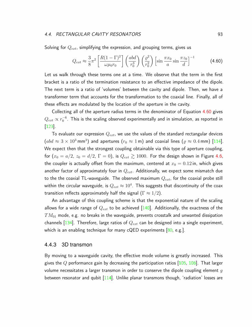
4.4. RECTANGULAR CAVITY RESONATORS 93
Solving for Qext, simplifying the expression, and grouping terms, gives us
Qext ≈3
8π2
[R(1− Γ)2
ωµ0r0
](abd
r30
)(%2
r20
)[sin
πx0
asin
πz0
d
]−1
(4.60)
Let us walk through these terms one at a time. We observe that the term in the firstbracket is a ratio of the termination resistance to an effective impedance of the dipole.The next term is a ratio of ‘volumes’ between the cavity and dipole. Then, we have atransformer term that accounts for the transformation to the coaxial line. Finally, all ofthese effects are modulated by the location of the aperture in the cavity.
Collecting all of the aperture radius terms in the denominator of Equation 4.60 givesQext ∝ r−6
0 . This is the scaling observed experimentally and in simulation, as reported in[123].
To evaluate our expression Qext, we use the values of the standard rectangular devices(abd ≈ 3 × 103 mm3) and apertures (r0 ≈ 1m) and coaxial lines (% ≈ 0.4mm) [114].We expect then that the strongest coupling obtainable via this type of aperture coupling,for (x0 = a/2, z0 = d/2, Γ = 0), is Qext & 1000. For the design shown in Figure 4.6,the coupler is actually offset from the maximum, centered at x0 = 0.12 in, which givesanother factor of approximately four in Qext. Additionally, we expect some mismatch dueto the the coaxial TL-waveguide. The observed maximum Qext, for the coaxial probe stillwithin the circular waveguide, is Qext ≈ 104. This suggests that discontinuity of the coaxtransition reflects approximately half the signal (Γ ≈ 1/2).
An advantage of this coupling scheme is that the exponential nature of the scalingallows for a wide range of Qext to be achieved [140]. Additionally, the exactness of theTM01 mode, e.g. no breaks in the waveguide, prevents crosstalk and unwanted dissipationchannels [134]. Therefore, large ratios of Qext can be designed into a single experiment,which is an enabling technique for many cQED experiments [80, e.g.].
4.4.3 3D transmon
By moving to a waveguide cavity, the effective mode volume is greatly increased. Thisgives the Q performance gain by decreasing the participation ratios [105, 106]. That largervolume necessitates a larger transmon in order to conserve the dipole coupling element gbetween resonator and qubit [114]. Unlike planar transmons though, ‘radiation’ losses are
4.4. RECTANGULAR CAVITY RESONATORS 94
suppressed by the fact that the ‘package’ of the 3D cavity is the resonator itself. Therefore,only the Hamiltonian dictates the size constraints on the device.
The 3D transmon has longer coherence (T1 ∼ T2 ∼ 100µs) than other superconductingqubits, likely for several reasons [114, 141]. First, rectangular waveguide cavities presenta relatively a ‘clean’ RF environment for the transmon. In comparison to the packagingfor planar transmons, the qubit sees no wirebonds, epoxy, or circuit board, all of whichcould present dissipation to planar transmons [62]. In addition, the larger dimensions ofthe 3D transmon are beneficial to the participation ratios of the mode [105, 106]. Precisecalculations show that 3D transmons can be less sensitive to surface dielectric loss andto quasiparticles by an order of magnitude [105]. If these loss mechanisms are the rootcause of dissipation in planar transmons, a similar factor for an improvement in lifetimeshould accompany the 3D transmon. Finally, the two transmon regimes store energy intheir substrates at approximately equal proportions. Encouragingly, the high coherenceobtained in 3D transmons effectively rules out bulk dielectric loss as a limiting factor forplanar devices at their observed values.
‘Scaling-up’ 3D transmon circuits is one sense as easy as for planar circuits. Forinstance, [Sears APS] has shown preliminary results from an 3D architecture which has48 transmon elements coupled to a single 3D cavity [142]. Implementing individual qubitcontrol and readout with this architecture might be more of a challenge since the ‘emptybox’ approach of rectangular cavities lends itself mostly to always-on couplings. Yet, cleverproposals exist for leveraging that type of coupling for tailoring subsets of multi-qubitmeasurements as well as constructing many-qubit gates [143]. The 3D transmon thus posesa viable architecture for next-generation experiments with multi-qubit parity eigenstatesand error correction [144].
Moreover, the flexibility of the 3D architecture lends itself to creativity in experimentalimplementation. For instance, waveguide Purcell filters have been integrated in such devicesand exhibit fundamentally new spectral filtering [60]. These filters have led to recordfidelities for QND measurements on cQED systems [60]. Having access to a 3D-distributedmode has made it possible to couple 3D transmons to new degrees of freedom, suchas ferromagnetic magnons [145], opening the door to using new, coherent systems asquantum memories of transmon qubits [49, and references therein].
Finally, the 3D transmon can also be taken as a proof-of-principle demonstration thatsolid state qubits can be coupled to waveguide cavities, which themselves are interestingobjects. Superconducting cavities can be significantly longer lived that state-of-the-art

4.4. RECTANGULAR CAVITY RESONATORS 95
superconducting qubits [116], reaching single photon lifetimes as long as 100ms [146]. Ifthese lifetimes can be combined with the strong coupling of cQED, a number of fascinatingconsequences will immediately follow, the first likely being the realization of extremelyeffective quantum memories [49]. However, as we show in the next subsection, therectangular waveguide architecture might not be sufficiently robust for this vision.
4.4.4 Losses
Because the fields of a rectangular waveguide are analytically solvable, we can determinewhat dissipation is introduced to a rectangular cavity by a given loss mechanism. To simplifyour discussion, we take the rectangular cavity dimensions (a = 17.8mm, b = 5.1mm,d = 35.6mm) [114] for this discussion.
Dielectric loss
Consider a layer of lossy dielectric on the walls of our cavity. For the TE101 mode, thefield is constant in y. Therefore, the (x, z) integrals in the definition of pdiel drop, leavingsimply
pdiel =2toxεrb
(4.61)
where tox and εr are the thickness and relative dielectric constant of the dielectric layer.For typical assumptions [105], tox = 3 nm, εr = 10 and resonator size b = 5mm, we findpdiel ∼ 10−7. Therefore, a bad dielectric qdiel ∼ 10 will limit these devices at the Q ∼ 108
level.
Conductor loss
Similarly, the sensitivity to quasiparticles is readily available [100]. The integrals in pmag
are straightforward to evaluate using the definitions for Hx and Hz in Equation 4.37 giving
pmag =ω0µ0λ
η
2π2(2a3b+ 2bd3 + a3d+ ad3)
(kad)3b. (4.62)
For a penetration depth of 50 nm [100], we have a magnetic participation ratio of pmag =
3× 10⁻⁵.

4.4. RECTANGULAR CAVITY RESONATORS 96
Surfa
ce c
urre
nt (J
/J0)
1.0
-1.0
0
0.5
-0.5
Distance (x/a)0 10.5
substrate
Figure 4.8: Perturbation of surface currents induced by substrate. The otherwise-sinusoidal surface currents acquire a sharp kink by the perturbation of the substrate. The slopeof this curve is essentially the sensitivity to asymmetry for seam dissipation as Equation 4.64,which is significantly steeper than the unperturbed resonant mode.
Seam loss
Finally, the sensitivity of rectangular cavities to dissipative seams can be calculated as well[123]. Let us first assume that the two halves of the cavity are joined together in the y− zplane as shown in Figure 4.6 [114]. The magnetic field terms that contribute to y∅ arethose parallel to the seam. Along the seam at z = 0, d however, this component would beHy, which is zero for the TE101 mode. Therefore, the relevant integral is only along then = y plane, where Hz is nonzero. We have then that
y∅ =1
ωµ0
2∫|Hz|2dl∫|H|2dV
=1
ωµ0
2(
πkηa
cos πx∅a
)22dπ
(abd/(16η2))
=1
ωµ0
(64π
k2a3b
)[cos(πx∅
a
)]2
(4.63)
For the choice of seam location x∅ = a/2 (as we do in practice) the seam admittancegoes to zero. Therefore, the design of the rectangular cavity is ideally such that nosurface currents flow across the seam. However, we expect a machining accuracy of upto δx ∼50µm for these parts as the result with careful machining techniques. We can

4.5. CYLINDRICAL CAVITY RESONATORS 97
approximate that the seam is located at x∅ = a/2 + δx. The resulting seam participationis
y∅ ≈1
ωµ0
(64π3
k2a3b
)(δx∅a
)2
. (4.64)
With the expected machining accuracy, we find that y∅ ≈ 1.8 /Ωm.This result is actually quite alarming. For the rectangular geometry and aluminum
cavity assembly process, we have ‘calibrated’ our gseam by taking several measurements ofquality factors at different, intentional δx values [123]. We find there that for aluminumgseam ≈ 104 /Ωm. Therefore, asymmetry at the level of machining tolerance may play adominant role in rectangular cavities at the Q∅ ≈ 5× 10⁷. Strikingly, this is average valuefor measured Qtot in high purity aluminum, indicating that assembly may so far be theultimate limit of these cavities.
An observation that made a substantial impact on the direction of this thesis is thatthe effect of seam loss is enhanced, as shown in Figure 4.8, by the presence of the dielectricsubstrate of the 3D transmon. This perturbation concentrates the surface currents atthe location of the substrate, which is also usually also the location of the seam. Theconcentrated currents account for a factor of approximately ten in the slope of the cosineof Hz locally, which is equivalent to a factor of 100 in y∅. For a fixed seam quality, amachining tolerance of δx ∼50µm would therefore be expected to limit cavities at thelevel of Q∅ ≈ 5 × 10⁵, which is near the observed values for Qtot for sapphire-loadedcavities. Simulations suggest that factors of two in Q∅ are possible for smaller pieces ofdielectric. Rethinking the mode structure is therefore important for extending Qtot > 107
in the presence of dielectric and seams.
4.5 Cylindrical cavity resonators
In order to avoid the issues of assembly, a new type of cavity was explored for cQEDapplications in this thesis [100]. We point out that is no coincidence that the long historyof high quality factor cavity resonators began with measurements on cylindrical [147, andreferences therein]. In particular, it was recognized that one mode of these boxes, theTE011 mode [148], has no dielectric participation pdiel = 0 and zero currents flowing acrossthe corners of the geometry. The latter observation allows the cylindrical cavity to beassembled as in Figure 4.9, with joints at the corners of the cylinder, such that pseam=0.

4.5. CYLINDRICAL CAVITY RESONATORS 98
By design, we are left with only conductor loss to limit the internal quality factor of theresonator [148].
With the rectangular cavities, we found that working with higher purity aluminum, andtreating the surfaces before measurement, higher quality factors can be achieved [100].Cylindrical cavities were developed during this thesis to probe what materials propertieswere improved via this technique, and moreover, if the extremely high quality factorsQ > 108 were achievable in a standard cQED experimental setup. These type of resonatorsmay eventually provide access to very long-lived resources in full cQED experiments.However, their primary purpose here is a platform for materials testing. At the conclusionof this section, we present a number of challenges that a cQED experimentalist facestoward qubit-integration.
4.5.1 Resonant modes
The fields of the TE011 mode are [111, op. cit. Eq. 6.54]
Hz = H0J0(p11ρ
a) sin
πz
d(4.65a)
Hρ = −βaH0
p11
J1(p11ρ
a) cos
πz
d(4.65b)
Eφ = −jkηaH0
p11
J1(p11ρ
a) sin
πz
d, (4.65c)
where a is the radius, d is the height, and as before pnm is the mth zero of Jn(x)
(p11 ≈ 3.83). Immediately, we recognize that at the side walls (ρ = a), J1(p11) = 0
implies that the electric field is zero there. In addition, on the lid (z = 0, d), sin(0) = 0 orsin π = 0 gives zero electric field there, too. Therefore, the electric field vanishes at allcavity surfaces. Hence,
pdiel = 0. (4.66)
Furthermore, at the corners of the geometry, (z = 0, d) and (ρ = a), we have that
Hz
∣∣∣corner
= Hρ
∣∣∣corner
= 0. (4.67)
Therefore, a joint located at the corners of this cavity has y∅ = 0 for this special mode.Combining these two ideas we thus expect the TE011 mode to be solely limited by conductorloss [148]. Furthermore, because of the large volume to surface ratio of the mode, we

4.5. CYLINDRICAL CAVITY RESONATORS 99
expect pmag to be quite small. For all of these reasons, we expect that the TE011 modeshould indeed achieve high Qtot.
Additionally, the cylindrical geometry supports a diversity of modes whose ordering canbe altered by the ratio of the cavity diameter to its height [111]. However, at best, theTE011 mode is the sixth lowest mode [111, op. cit. Fig. 6.9]. The frequency of the modeis given by
f0 =c
2π
√(p11
a
)2
+(πzd
)2
(4.68)
Since J ′0(x) = −J1(x) though p11 is essentially double-counted in the ordering of modes[148]. Therefore, the TE011 is degenerate with pair of TM111 modes for all aspect ratiosof cavity.
We use a shape perturbation to split this degeneracy [100]. We introduce a ring-shapedextrusion to the mode at the corners (visible in Fig. 4.9). There, the TE011 mode is largelyunaffected, while the TM111 experiences an effectively smaller volume. We can calculatethe expected shift for small perturbations [111, op. cit. Eq. 6.103] as
δω0
ω0
≈ δWm − δWe
Wtot
. (4.69)
Our ring has a rectangular cross section (w × w) so that
δWm ≈ 2µ0w3
∫|Hφ(ρ = a, z = 0, φ)|2dφ
=2πµ0a
2w3
(p11)2[ω0ε0E0J2(p11)]2 .
(4.70)
Whereas, the total energy is
Wtot =πµ0a
4d
8(p11)2[ω0ε0E0J2(p11)]2 . (4.71)
The ratio therefore givesδω0
ω0
≈ 16w3
a2d. (4.72)
We seek to perturb the modes only modestly (δω0/ω0 ∼ 0.1%) and therefore, choosew = 0.032 in. The above expression would predict an induced detuning of the modesof δω0/2π ≈ 10MHz for a = 0.75 in, d = 0.95 in, and ω0/2π = 11.5GHz. However,other effects, such as asymmetry introduced by machining imprecision, can further split

4.5. CYLINDRICAL CAVITY RESONATORS 100
SMA teeRF in RF out
coupler
E H
(a) (b)
field10
Figure 4.9: Cylindrical TE011 resonator. (a) Field distribution of the TE011 mode. Theelectric field is concentrated in a torus about the cylindrical zaxis, and the electric fieldvectors point along φ. It is visible on the plot that the electric field goes to zero on all thecavity wall. The magnetic field is zero at the the corners of the cavity and a maximum at thecenter. (b) Physical realization of the cylindrical cavity. Two lids close the cylindrical cavityalong the region of minimum magnetic field. Additionally, the small ring perturbation on thelids, which detunes the degenerate TM111 modes, is visible. An SMA tee allows this cavityto be measured with the shunt technique. The coupling from SMA to cavity is accomplishedvia a loop coupler as described in Section 4.5.2. (Figure used with permission from [100].See Copyright Permissions.)
degeneracies at this small of a limit. The above estimates serve as a lower bound then forthe splitting between modes. Experimentally, we observe a detuning between TE011 andTM111 modes of δω/2π ≈ 30MHz.
The other modes of the cylinder are useful to study many dissipation mechanisms atonce, since they will all have various sensitivities to materials and assembly. For instance,if the TE011 mode is significantly higher Q than any of these other modes, we require lossmechanisms beyond conductor loss to explain the other modes (see Table 4.2) [100].
4.5.2 Input-output coupling
As shown in Figure 4.10, coupling to the cylindrical cavity is achieved in a similar manneras before (see Sec. 4.4.2). However, due to the special configuration of the TE011 mode,magnetic dipole coupling is required here. Additionally, several other considerations are

4.5. CYLINDRICAL CAVITY RESONATORS 101
L
TEM TE11 M•H
E×H*
(a) (b)
TE011
Figure 4.10: Input-output coupling for cylindrical cavities. (a) Coupling to the cylin-drical TE011 is accomplished in an analogous manner to the rectangular cavity geometry.The center pin of a coaxial cable is soldered to the outer shield, forming a loop. The dipolemoment of the loop is aligned to the local orientation of the magnetic field of the cavity.A propagating circulating waveguide mode (TE11) translates this dipole moment to theresonator with an exponentially reduced amplitude. (b) A circular aperture acts as magneticdipole in the cavity.
taken into account when implementing a coupling scheme for the cylindrical cavity. Inparticular, the presence of the TM111 modes necessitates caution. This section providesan overview of these choices.
In general, the coupling design problem begins with selecting which field component ofthe resonator to excite. For the TE011 mode, only Hρ is remains nonzero at the lids ofthe cavity, where machining is easiest. Furthermore, Hρ has its maximum at ρ/a = 0.48,making this location particularly attractive.
To couple to the cavity’s Hρ, we must choose which sub-cutoff waveguide mode toexcite. We treat the cavity’s field as a constant vector across the face of our sub-cutoffwaveguide (magnetic dipole approximation) [137]. In the cylindrical coordinate frame ofthe sub-cutoff waveguide, the magnetic field therefore actually reverses polarity under (φ′
⇒ -ρ′). Therefore, only those propagating modes with Hρ′ that changes polarity under

4.5. CYLINDRICAL CAVITY RESONATORS 102
this transformation will contribute to this coupling scheme. Looking at the Hρ′ componentof our propagating modes, we have
Hρ′,TE =−jβkc
cos(nφ)J ′n(kcρ′) (4.73)
Hρ′,TM =−jωεnk2cρ
sin(nφ)Jn(kcρ′) (4.74)
A loop or iris has a magnetic moment that is constant in the direction of its orientation(surface area n for the loop) as pictured in [138, op. cit. Fig. 4.32]. Therefore, we alignthe coupling loop to the ρ vector of the cavity [100]. Actually, this orientation couples toboth TEnm and TMnm modes. Therefore, we need to consider all propagating modes.
In the experimental realization, the sub-cutoff waveguide has a radius r= 1.8mm,which sets a propagation constant for each mode (calculated explicitly in Appendix C).As for the rectangular cavity (Section 4.4.2), we expect the lowest mode to dominatethe transport. We observe that the propagation constant for the TE11 mode is about afactor of two smaller than that of the next-lowest mode, the TM11 mode. Therefore, weexpect the TE11 mode to propagate signals in and out of the cavity. Thus for the cavity’sresonant TE011 mode, the scaling of Qext should be
Qext ∝ e2βTE11L, (4.75)
which is the scaling observed experimentally (Appendix C).
4.5.3 Losses
The formulas for three main participation ratios for general TEnml and TMnml modes aregiven in Appendix D. We give the specific expressions for the TE011 here for completeness.We calculate the losses for a resonator with radius a and height d.
Dielectric loss
The dielectric participation ratio is exactly zero for a TE011 mode. Introducing the shapeperturbation to the cavity causes some electric field to reach the walls of the geometry.Finite element techniques are the most accurate method for determining the resulting pdiel.For the implemented geometry, we have pdiel ≈ 4 × 10⁻¹¹. Therefore, an unphysically

4.5. CYLINDRICAL CAVITY RESONATORS 103
low qdiel would be necessary to damp the TE011 mode at the levels we observe (Q . 109)[100].
Conductor loss
The magnetic participation ratio is [138, op. cit. Eq 7.55]
pmag =2ωµ0λ
η
[(p11)2 + 2π2a3
d3
][(p11)2 +
(πad
)2]3/2
(4.76)
which gives pmag = 6× 10⁻⁶ [100]. A measured Qtot = 7× 10⁸ for this mode puts ourbest bound on qcond & 4× 10³.
Seam loss
We do not rely on stringent machining tolerances to achieve zero surface currents atthe seams for the TE011 mode. However, other modes in the cylindrical resonator doparticipate with this loss mechanism. We give expressions for the seam-admittances ofthese modes in Appendix D since these also shed light on other geometries which rely onsmall g∅.
4.5.4 Hurdles to transmon integration
Despite the high quality factors achieved for the TE011 mode, several obstacles must beovercome in order to successfully integrate this mode with a transmon. The first of theseissues is the frequency spectrum of cylindrical cavities [111]. As previously described, theTE011 mode is not the fundamental mode of the cylindrical cavity. Therefore, any cQEDexperiment must deal with multi-mode dynamics, and these modes will lie below any lowpass filtering. Moreover, the degenerate TM111 modes, which are lower Q, will always bea nuisance for large-bandwidth pulses that are typically used to control resonators.
Beyond the spectral concerns, the field pattern of the TE011 is not obviously beneficial forcQED. The geometry has a larger mode-volume than the rectangular cavities, necessitatinga larger transmon to maintain strong coupling. Also, the toroidal electric fields, with fieldvectors along φ, makes the standard electric-dipole coupling difficult in the limit of largedipoles. The location of the field maxima in the interior of the cavity further requires alarge amount of sapphire to be loaded into the cavity for strong coupling.
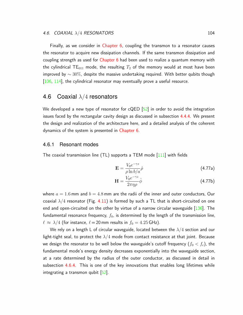
4.6. COAXIAL λ/4 RESONATORS 104
Finally, as we consider in Chapter 6, coupling the transmon to a resonator causesthe resonator to acquire new dissipation channels. If the same transmon dissipation andcoupling strength as used for Chapter 6 had been used to realize a quantum memory withthe cylindrical TE011 mode, the resulting T2 of the memory would at most have beenimproved by ∼ 30%, despite the massive undertaking required. With better qubits though[106, 114], the cylindrical resonator may eventually prove a useful resource.
4.6 Coaxial λ/4 resonators
We developed a new type of resonator for cQED [52] in order to avoid the integrationissues faced by the rectangular cavity design as discussed in subsection 4.4.4. We presentthe design and realization of the architecture here, and a detailed analysis of the coherentdynamics of the system is presented in Chapter 6.
4.6.1 Resonant modes
The coaxial transmission line (TL) supports a TEM mode [111] with fields
E =V0e
−γz
ρ ln b/aρ (4.77a)
H =V0e
−γz
2πηρφ (4.77b)
where a = 1.6mm and b = 4.8mm are the radii of the inner and outer conductors, Ourcoaxial λ/4 resonator (Fig. 4.11) is formed by such a TL that is short-circuited on oneend and open-circuited on the other by virtue of a narrow circular waveguide [136]. Thefundamental resonance frequency, f0, is determined by the length of the transmission line,` ≈ λ/4 (for instance, `=20mm results in f0 = 4.25GHz).
We rely on a length L of circular waveguide, located between the λ/4 section and ourlight-tight seal, to protect the λ/4 mode from contact resistance at that joint. Becausewe design the resonator to be well below the waveguide’s cutoff frequency (f0 < fc), thefundamental mode’s energy density decreases exponentially into the waveguide section,at a rate determined by the radius of the outer conductor, as discussed in detail insubsection 4.6.4. This is one of the key innovations that enables long lifetimes whileintegrating a transmon qubit [52].

4.6. COAXIAL λ/4 RESONATORS 105
1 mm
100 nm
(a) (b)
(c)
AlOx
Al Alλ/4
e-βz
L
E
p
Figure 4.11: Coaxial λ/4 resonator. (a) A quarter-wave coaxial resonator is definedby shorting a coaxial transmission line’s inner and outer conductors at one location on thetransmission line (bottom) and open-circuiting the line a distance λ/4 away (upward). Asuperconducting transmon qubit (green) can be coupled to the λ/4 mode by aligning theelectric dipole moment of the transmon −→p to the electric field of the resonator
−→E . In the
section above the coaxial resonator, the outer conductor’s cylindrical waveguide TE/TMmodes are well below cutoff. Placing a light-tight seam a distance L away from the resonatorthus allows the perturbation to be exponentially eliminated. This is the same effect asdescribed in Section 4.4.2. (b) A superconducting transmon qubit on sapphire (green) isinserted through a 1.5 mm hole. The qubit is also coupled to a second cavity used forreadout that is not shown here. (c) Electron beam microscopy image of a Josephson junctionthat provides the nonlinearity to the system. (Figure used with permission from [52]. SeeCopyright Permissions.)
Because the cavity is a λ/4 resonator, we expect the next transmission line mode atf0 ≈ 3λ/4. The separation in frequency between the fundamental mode and the next TEMharmonic is actually double the fundamental frequency itself, which provides a remarkably‘clean’ spectrum. In fact, waveguide modes of the coax, in particular the TE11 mode, canbe lower-lying than the second TEM harmonic. The TE11 mode begins to play a role whenω ≈ 2c/(a + b) = (2π) × 15GHz. Simulations show that these box modes do indeedappear at ω0/2π ≈ 18GHz.
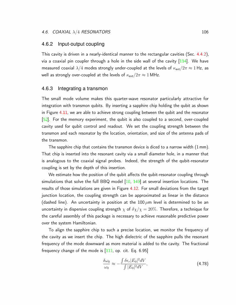
4.6. COAXIAL λ/4 RESONATORS 106
4.6.2 Input-output coupling
This cavity is driven in a nearly-identical manner to the rectangular cavities (Sec. 4.4.2),via a coaxial pin coupler through a hole in the side wall of the cavity [114]. We havemeasured coaxial λ/4 modes strongly under-coupled at the levels of κext/2π ≈ 1Hz, aswell as strongly over-coupled at the levels of κext/2π ≈ 1MHz.
4.6.3 Integrating a transmon
The small mode volume makes this quarter-wave resonator particularly attractive forintegration with transmon qubits. By inserting a sapphire chip holding the qubit as shownin Figure 4.11, we are able to achieve strong coupling between the qubit and the resonator[52]. For the memory experiment, the qubit is also coupled to a second, over-coupledcavity used for qubit control and readout. We set the coupling strength between thetransmon and each resonator by the location, orientation, and size of the antenna pads ofthe transmon.
The sapphire chip that contains the transmon device is diced to a narrow width (1mm).That chip is inserted into the resonant cavity via a small diameter hole, in a manner thatis analogous to the coaxial signal probes. Indeed, the strength of the qubit-resonatorcoupling is set by the depth of this insertion.
We estimate how the position of the qubit affects the qubit-resonator coupling throughsimulations that solve the full BBQ model [10, 149] at several insertion locations. Theresults of those simulations are given in Figure 4.12. For small deviations from the targetjunction location, the coupling strength can be approximated as linear in the distance(dashed line). An uncertainty in position at the 100µm level is determined to be anuncertainty in dispersive coupling strength χ of δχ/χ = 20%. Therefore, a technique forthe careful assembly of this package is necessary to achieve reasonable predictive powerover the system Hamiltonian.
To align the sapphire chip to such a precise location, we monitor the frequency ofthe cavity as we insert the chip. The high dielectric of the sapphire pulls the resonantfrequency of the mode downward as more material is added to the cavity. The fractionalfrequency change of the mode is [111, op. cit. Eq. 6.95]
δω0
ω0
≈ −∫δεr|E0|2dV∫|E0|2dV
, (4.78)

4.6. COAXIAL λ/4 RESONATORS 107
−400 −200 0 200 400Position (μm)
−1.0−0.5
0.00.51.01.52.0
Cou
plin
g (δχ
/χ)
4.16 4.19 4.22 4.25 4.28Frequency (GHz)
−60−50−40−30−20−10
S21
(dB)
simulatedparameters
room-temperature
increasedloading
(i)(ii)
(iii)
(a)
(b)
Figure 4.12: Assembling a coaxial quarter-wave cQED device. (a) Simulations providea means for estimating how the system’s degree of freedom in transmon location affect thedispersive coupling strength χ between the transmon and resonator. For small deviations(δx0 . 0.2mm), we find a linear approximation (dashed line) for the change in χ asδχ/χ ≈ δx0/(0.5 mm). (b) To achieve this precision in the transmon location, we relyon the frequency pull of the sapphire dielectric on the resonator. We monitor the centerfrequency of the resonator empty (i), with the sapphire fully inserted (iii), and for the finalassembled device (iii). Equation 4.79 is used to solve for the resulting transmon location.

4.6. COAXIAL λ/4 RESONATORS 108
where δεr = 9.4 for sapphire. We evaluate the above integral assuming that the field isconstant across a width w and thickness t of the substrate, giving
δω0
ω0
≈ − δεrwt
π`(ln(b/a))2
(1
x− 1
b
). (4.79)
where x is the extent of the sapphire into the cavity. This expression holds whenever themode is not significantly distorted by the presence of the dielectric. Remarkably though,Equation 4.79 predicts the correct frequency shift for the sapphire fully inserted in theresonator (x = a), with the above expression giving δω0/2π ≈ 107MHz as comparedthe observed value δω0/2π = 93MHz. In fact, the 15% frequency difference equates toapproximately 50µm of location uncertainty, a difference that may arise from chippingand kerf uncertainty of the sapphire chip itself.
Table 4.1: Predicted and extracted parameters for the full device device Hamiltonian.
H/~ Experiment (Hz) Simulation (Hz) Deviation (%)ωs/2π 4.250 ×10⁹ 4.246 ×10⁹ < 1ωq/2π 7.906 ×10⁹ 7.878 ×10⁹ < 1ωr/2π 9.777 ×10⁹ 9.653 ×10⁹ 1χsq/2π 4.99 ×10⁵ 5.56 ×10⁵ 11χrq/2π 8.25 ×10⁵ 7.77 ×10⁵ 6χsr/2π - 1.60 ×10³ -Ks/2π 4.50 ×10² 5.20 ×10² 16Kq/2π 1.46 ×10⁸ 1.41 ×10⁸ 3Kr/2π - 1.20 ×10³ -
As shown in Figure 4.12, we can use Equation 4.79 to solve for the sapphire locationfor a given assembly. This process can be done iteratively at room-temperature. However,we caution the reader that low VNA powers (. −40 dB) should be used for this techniqueto avoid breaking the AlOx tunnel junction. The achieved transmon parameters are listedin Table 4.2.

4.6. COAXIAL λ/4 RESONATORS 109
4.6.4 Losses
The dimensions for the inner and outer conductors for the coax resonator are a = 1.6mmand b = 4.8mm respectively [52]. We calculate the participation ratios for the fundamentalmode here.
Dielectric loss
The dielectric participation ratio for the coaxial cavity is
pdiel ≈toxεr,ox
(1
a ln(b/a)
)(4.80)
For the standard assumptions, tox = 3 nm and εr,ox = 10 and our geometry we havepdiel ≈ 2× 10⁻⁷.
Conductor loss
The magnetic participation ratio for the coaxial cavity is
pdiel ≈ λ
(1
a ln(b/a)
)(4.81)
For the standard λ = 50 nm and our geometry we have pmag ≈ 4× 10⁻⁷.
Seam loss
If the ‘open-circuit’ termination of this resonator was exact, placing the seam locationanywhere above the center conductor of the coax would have zero seam-participation.However, the waveguide coupling weakens this effect. We use finite element techniques toevaluate y∅ numerically, finding y∅ = 1.3× 10⁻³ /Ωm at the interface of the transmissionline and waveguide sections. We expect y∅ to decay exactly as Qext, as described insection 4.4.2, except with a different e-folding length.
The TM01 mode sets the λ/4 mode’s propagation into the waveguide. The evanescentTM01 mode has a propagation constant β =
√k2 − (2.41/a)2, where k = 2π/λ is the
wavenumber, and a = 5mm is the radius of the circular waveguide section. At ourtransmission line’s fundamental resonance frequency of 4.25 GHz, the propagation constantis β = ı/2.03mm, below cutoff. Therefore, the λ/4 mode’s current-energy density falls

4.7. SUMMARY OF MODES AND QUALITY FACTORS 110
as |H|2 ∝ e−2|β|z into the waveguide section. Finite element simulations, which take intoaccount all possible waveguide modes, confirm these simple predictions to within 5%.
We seal the cavity for light-tightness after a length of waveguide section that isL ≈ 10/|β|. The resonator’s energy has been suppressed at this location by a factorof about e−20. We therefore rule out assembly defects such as contact resistance as apotentially limiting dissipation mechanism at internal quality factors of Qint ∼ 109.
4.7 Summary of modes and quality factors
In Table 4.2, we provide a compiled list of the different types of resonators presented inthis chapter and the observed quality factors of each mode. As is clear from the table,the TE011 has essentially no sensitivity to dielectrics and seams. Conductor loss is themain culprit for the dissipation of this mode. Therefore, the bound on qmag obtainedfrom these experiments is potentially a real measure of the conductivity of our high purity,machined aluminum. It is interesting then that the coaxial λ/4 cavities achieve very similarbounds for qmag. We can deduce by this comparison that the λ/4 cavities are likely alsolimited by conductor loss. Vortices and nonequilibrium quasiparticles are known to causeconductor loss in superconductors. Investigating these loss mechanisms could be a fruitfulpath forward for improving these devices further.

4.7. SUMMARY OF MODES AND QUALITY FACTORS 111
Table 4.2: Resonant modes and quality factors for high purity aluminum.. Resultsfor rectangular cavities (R), cylindrical cavities (C), and coaxial λ/4 cavities (Q). All cavitieshave undergone the surface preparation described in Chapter 5. Material bounds (q ≥ org∅ ≥) are under the assumptions provided in Section 4.2. We use bold font to denote thebest bounds obtained. Unphysical bounds are left as a dash.
Device Mode f0 (GHz) Qint qdiel qmag g∅(/Ωm) citeR1 TE101 9.455 4.2×10⁷ 5.0 1.3×10³ 7.8×10³ [100]R2 TE101 9.481 4.3×10⁷ 5.1 1.3×10³ 7.9×10³ [100]R2 TE101 9.481 6.9×10⁷ 8.1 2.1×10³ 1.3×10⁴ [100]C1 TE111 7.700 3.1×10⁷ - 3.4×10² 1.0× 10⁶ [100]C1 TM111 11.448 1.4×10⁷ - 2.3×10² 1.4×10⁵ [100]C1 TE011 11.417 6.1×10⁸ - 3.7×10³ - [100]C2 TE011 11.440 7.4×10⁸ - 4.5×10³ - [100]C2 TE011 11.442 5.2×10⁸ - 3.2×10³ - [100]Q1 λ/4 7.881 8.7×10⁷ 20. 3.3×10³ -Q2 λ/4 7.858 8.6×10⁷ 20. 3.3×10³ -Q3 λ/4 7.992 8.0×10⁷ 18. 3.0×10³ -Q4 λ/4 4.280 7.0×10⁷ 16. 2.7×10³ - [52]

CHAPTER 5
Measuring resonators and transmons
This chapter presents the core cQED techniques used throughout this thesis. Two basictypes of measurements are considered. First, we present the characterization of linear
resonators that are intended for use in full cQED devices. How to achieve high qualityfactors, as well as how to extract Q from measurements, is presented in detail. Then, wediscuss methods for transmon experiments. We focus here on experiments that illuminateproperties of a transmon as an individual circuit element. The next chapter concerns thecoupling between a transmon and a resonator, as well as new experiments enabled by thecoupling (besides qubit readout), in detail.
Many of the techniques in this chapter have a long history in cQED. For a complimentaryreview of techniques for resonator measurements, we refer the reader to Geerlings’s thesis[110]. A step-by-step manual for transmon characterization can be found in Sears’s thesis[43], and many transmon control techniques are presented in detail in Reed’s thesis [144].However, a number of new techniques are also explored here.
5.1 Linear resonator experiments
Being able to fabricate and probe high quality bare resonators (Q > 108) is an importantstep toward using such objects as coherent quantum memories for cQED [100]. Moreover,their existence in standard cQED setups (dilution refrigerator, coaxial input-output lines,
112

5.1. LINEAR RESONATOR EXPERIMENTS 113
etc.), shows that there are not fundamental barriers to these long lifetimes using thetechnology already common for cQED experiments. Additionally, resonators can besensitive to the same dissipation mechanisms that may limit qubits. Optimizing resonatorperformance can therefore be a powerful path forward for improving qubits [104].
In this section, we describe the methods to prepare, measure, and analyze superconduct-ing aluminum cavity resonators [100]. Preparing these cavities for cryogenic measurementinvolves a surface etching step, calibrating the microwave couplers, and finally, integratingthe cavities into a dilution refrigerator measurement setup. The central technique forvetting the performance of a superconducting cavity is via measurements with a VectorNetwork Analyzer (VNA) in a quasi-reflection mode. Fully interpreting these measurementsis only possible by repeating them across a range of circulating RF energies and elevatedtemperatures since a resonator’s sensitivity to loss mechanisms, such as quasiparticle loss,can be revealed through these schemes.
5.1.1 Surface preparation
In order to achieve the highest quality factors in superconducting niobium cavity resonators,it has been commonly observed that 100-200µm of surface layer should be removed priorto those measurements [147]. Preparing superconducting surfaces via etching has been awell-established technique for niobium cavities used in particle accelerators [147]. There, acombination of buffered chemical polishing (BCP) and electro-polishing (EP) is used tomitigate a damaged surface layer.
For high purity aluminum (& 99.99% pure), we have found that chemically etchingcavities is essential to realize their optimum performance [100]. The commercially availableAluminum Etch A by Transene Co is a combination of nitric and phosphoric acid thathas an etch rate of pure aluminum of 100 Å/s at 50·C [150]. The nitric acid attacksthe aluminum directly, which results in an aluminum oxide layer that is dissolved by thephosphoric acid [151], as
7A + 5HNO3 + 21H3PO4 ⇒ +7Al(H2PO4)3 + 13H2O + 2N2 + NO2. (5.1)
These alternating processes should remove 150µm of material in approximately four hours.However, the etch rate for is highly dependent on temperature (550 Å/s at 75C) and theprocess is exothermal [151]. Therefore, care must be taken to measure the total etch ratefor a given setup.

5.1. LINEAR RESONATOR EXPERIMENTS 114
(a) (b)
(c) (d)
Figure 5.1: Surface preparation of superconducting cavities. (a) A high purity alu-minum cavity is placed in a bath of Aluminum Etch A to remove the damaged surface layer.This process is conducted on a hot plate in the vented acid bench of the Becton cleanroom.Nested beakers with an additional lid prevents overflow and contamination. (b) High purityaluminum sample before etching. Clear signs of machining scratches are visible. (c) Theacid bath at the end of a two-hour cycle. The liquid has been turned green by aluminumphosphate salt. Between the liquid and lid, nitrous oxide is trapped and vents in burstswhenever the pressure exceeds the weight of the lid. If the process is left to continue, thebath may eventually run clear again as a runaway reaction will begin to attack the salt itself.Unreliable etch rates and surface impedance results follow this runaway effect. (d) Aftertwo cycles of the two-hour process, the high purity sample is highly reflective with grainboundaries that are easily visible in the picture.
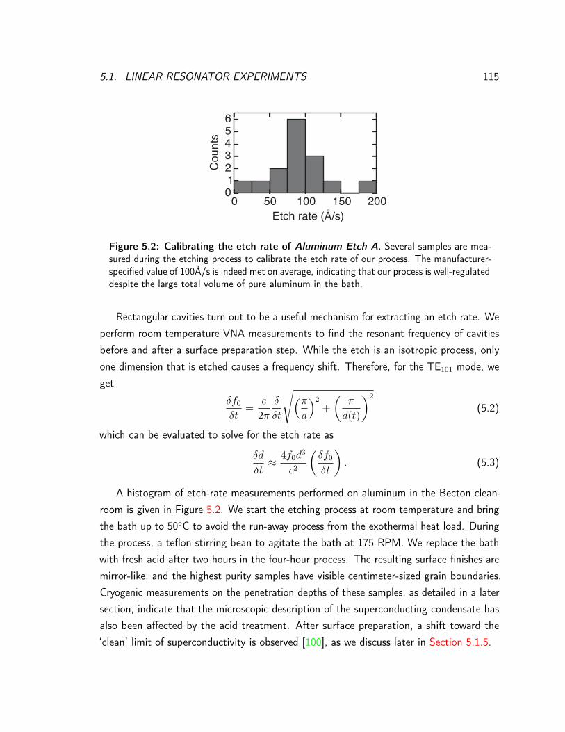
5.1. LINEAR RESONATOR EXPERIMENTS 115
0 50 100 150 200Etch rate (A/s)
0123456
Cou
nts
°
Figure 5.2: Calibrating the etch rate of Aluminum Etch A. Several samples are mea-sured during the etching process to calibrate the etch rate of our process. The manufacturer-specified value of 100Å/s is indeed met on average, indicating that our process is well-regulateddespite the large total volume of pure aluminum in the bath.
Rectangular cavities turn out to be a useful mechanism for extracting an etch rate. Weperform room temperature VNA measurements to find the resonant frequency of cavitiesbefore and after a surface preparation step. While the etch is an isotropic process, onlyone dimension that is etched causes a frequency shift. Therefore, for the TE101 mode, weget
δf0
δt=
c
2π
δ
δt
√(πa
)2
+
(π
d(t)
)2
(5.2)
which can be evaluated to solve for the etch rate as
δd
δt≈ 4f0d
3
c2
(δf0
δt
). (5.3)
A histogram of etch-rate measurements performed on aluminum in the Becton clean-room is given in Figure 5.2. We start the etching process at room temperature and bringthe bath up to 50C to avoid the run-away process from the exothermal heat load. Duringthe process, a teflon stirring bean to agitate the bath at 175 RPM. We replace the bathwith fresh acid after two hours in the four-hour process. The resulting surface finishes aremirror-like, and the highest purity samples have visible centimeter-sized grain boundaries.Cryogenic measurements on the penetration depths of these samples, as detailed in a latersection, indicate that the microscopic description of the superconducting condensate hasalso been affected by the acid treatment. After surface preparation, a shift toward the‘clean’ limit of superconductivity is observed [100], as we discuss later in Section 5.1.5.

5.1. LINEAR RESONATOR EXPERIMENTS 116
5.1.2 Resonator measurement setup
As pictured in Figure 5.3, the cavity quality factor measurements in this thesis and in [100]were performed with the resonators attached to the base (T ≈ 15 mK) cooling stage ofa dilution refrigerator. Stainless steel cables carry signals from room temperature to thebase stage. Physical attenuation of 20 dB and 30 dB is located on the 4K and base stagesto thermalize the input signals. The impedance of the device under study is introduced tothe signal chain by an SMA tee. The third port of the tee continues through two isolatorsand through superconducting coaxial cable to the 4K stage. At 4K, the signal passesthrough a low noise HEMT amplifier. Stainless steel cable carriers the signal to roomtemperature, where the output passes through two low noise Miteq amplifiers. The inputand output ports of this signal chain are measured in transmission via a vector networkanalyzer (VNA). This setup is similar to other quasi-transmission techniques as describedin Section 5.1.3.
The cavities are mounted on copper brackets that are bolted to the base plate of therefrigerator. These samples are housed in mu-metal shielding (Amuneal 4K) [62], and onlynonmagnetic components are used within the mu-metal shield to maintain low magneticfields. Probing the magnetic field near the sample with a calibrated magnetometer, wedetect field strengths of milligauss in the full measurement setup.
5.1.3 Extracting quality factors
The resonator measurement setup described in the previous subsection allows us to measurein the quasi-transmission method referred to as the shunt, hanger, or notch technique[104, 130, 133, 152]. Essentially, the signal-carrying transmission line is shunted by theimpedance of a resonator under study as shown in Figure 5.5. The scattering matrix canbe calculated taking into account imperfections, such as cable delay and reflections, thatarise from a lack of calibration in the cryogenic environment. The far off-resonant behaviorof these measurements serve as an in-situ calibration. Importantly, this calibration allowsus to extract the external and internal quality factors independently.
Several derivations for this technique have been presented in papers [130, 133, 152]and theses [110, 112]. We provide the main results here, beginning with the ideal shuntresonant circuit (Fig. 5.5). If it has no internal dissipation, the resonant circuit simply

5.1. LINEAR RESONATOR EXPERIMENTS 117
isolators (2x)
30 dB20 dB
HEM
T 4 K
15 mK
300 K
LO
reference
signalRF
cryoperm m
agnetic shield
SMA tee
vector network analyzer
Figure 5.3: Experimental schematic for resonator testing. To extract the quality factorof a resonator, phase-resolved (vector) network analysis is performed on a transmission linecircuit that includes the resonator. The analysis compares the full circuit response (largeloop) to a reference branch. Two generators are used to bring the measurement frequencydown to match an ADC digitizing rate. Cryogenic attenuators reduce the blackbody radiationfrom 300K. An SMA-tee is used to introduce the impedance of the resonator to the coaxialtransmission line. A low noise amplifier boosts the signal before the room temperatureamplification and demodulation.

5.1. LINEAR RESONATOR EXPERIMENTS 118
Figure 5.4: Picture of resonator payload. Three high purity aluminum coaxial resonatorsand two niobium TM010 cavities. Thermalization is provided by bolting each resonator toa copper bracket, which itself will be bolted to the mixing chamber. This payload will beinserted into a magnetic shield for measurement. Copper inner-outer coaxial cable is usedinside the shield, and non-magnetic RF and mechanical assembly components are used tomaintain milligauss fields inside the shield.
creates a phase interference effect in the transmitted signal that is a Lorentzian as
S21 = 1− κextκext + 2ı(ω − ω0)
(5.4)
Note that on resonance the phase inversion leads to complete destructive interference forthe outgoing signal (S21 = 0), regardless of the coupling strength κext. Essentially, thisresonator is always infinitely over coupled. If instead the resonator has a finite internalenergy decay rate (κint), the resonance frequency acquires an imaginary component [110],ω = ω0 + ıκint/2, to account for its lack of a natural frequency response. Now, thetransmitted signal is given by
S21 = 1− κextκext + κint + 2ı(ω − ω0)
, (5.5)
or using quality factors to re-parameterize the expression (Qtot ≡ ω/κtot), we have
S21 = 1− Qtot
Qext + 2ıQtotQext(ω/ω0 − 1). (5.6)

5.1. LINEAR RESONATOR EXPERIMENTS 119
(a)
Y1 Y2Port 1 Port 2
Re S21
Im S
21
0.0 1.00.5
0.0
-0.5
0.5
(b)
Re S21
Im S
21
0.0 0.5-0.5
0.0
-0.5
0.5
(c)
ω
Figure 5.5: Shunt resonances along a transmission line. (a). The two-port circuitof a resonator measured via the shunt-technique. For an ideal transmission line that hasno additional reflections or crosstalk, the other shunt impedances Y1, Y2 would be infinite.However, the response of the resonant circuit can be extracted for nearly-arbitrary Y1, Y2. (b)The transmission response of the ideal circuit. Far detuned from resonance, the transmissionis unaffected by the resonator (S21 = 1). Resonance traces out a circle on the complex planeof the transmitted signal (Re(S21, Im(S21)), the rate at which phase is acquired along thiscircle (θ[ω]) gives the total quality factor of the resonance. The distance from the origin atresonance gives the ratio of internal to external quality factors. For completely over-coupledresonators, the transmission approaches zero on resonance (purple). Critically coupled(Qint = Qext) gives transmission of one-half on resonance (blue). Finally, under-coupledresonances give transmission closer to unity (red). (c) Imperfections in the transmissionline Y1, Y2 cause displacements and rotations of the resonant circle. However importantly,the environmental admittances do not alter the rate of θ[ω], which gives the total qualityfactor. Moreover, these effects can be calibrated out by taking into account the far detunedtransmission, which gives access to the ratio of Qtot/Qext.

5.1. LINEAR RESONATOR EXPERIMENTS 120
In the complex transmitted voltages, the transmitted signal traces out a circle in the IQplane. To see why this is a circle, it is useful to define an angle [152]
θ(ω) = tan−1 [2Qtot(ω/ω0 − 1)] , (5.7)
so that the transmission signal is given by
S21 = 1− Qtot
Qext
(1
1− ı tan θ
). (5.8)
Bringing the imaginary component to the numerator and using the trigonometric identity1 + tan2 θ = sec2 θ, we have
S21 = 1− Qtot
Qext
(cos2 θ + ı cos θ sin θ
). (5.9)
Finally, using the double-angle identities,
cos2 θ =1
2(1 + cos 2θ)
cos θ sin θ =1
2sin 2θ,
(5.10)
we obtain a simple form for S21 as
S21 = 1− Qtot
2Qext
(1 + e2ıθ
). (5.11)
We recognize the diameter of the circle to be 2Qtot/Qext and from the transmission circle’sprogression along θ as a function of frequency, we obtain Qtot independently from Qext
[152]. Thus, we can completely determine our internal and external dissipation.Impedance mismatches, crosstalk and other imperfections in our measurement chain
can be accounted for by allowing an imaginary component of the external quality factorQext = Qexte
ıε [152]. Additionally, loss and the electric phase-delay accumulated throughthe meters of coaxial cable can be lumped into a single complex scaling term Gejωτ , whereτ is the electrical delay time and G is a complex gain term. These perturbation have theeffect of scaling, rotating, and displacing the resonant transmission circle while preservingthe separation of Qint and Qext. The imperfections can be combined [152] as
S21 = Gejωτ[1− Qtot
2Qext
(1 + e2ıθ
)e−ıε
]. (5.12)

5.1. LINEAR RESONATOR EXPERIMENTS 121
−600−400−200 0 200 400 600Detuning (Hz)
−25−20−15−10−5
|S21
|2 (dB
)
−600−400−200 0 200 400 600Detuning (Hz)
−3.5−3.0−2.5−2.0−1.5−1.0
Phas
e (ra
d)
−0.5 0.0 0.5 1.0Re(S21)
−1.0−0.8−0.6−0.4−0.2
0.00.20.4
Im(S
21)
(a) (b)
(c) (d)
−600−400−200 0 200 400 600Detuning (Hz)
−3−2−10123
Phas
e (ra
d)
ωω
Figure 5.6: Fitting quality factors on the complex plane. (a). Raw data for thetransmitted signal through a shunt resonator. Because the VNA cannot be calibrated directlyat the device, we must transform the signal in post-processing by the far detuned signallevels. (b) A convenient representation for the signal is to evaluate the best-fit circle alongthe parametric angle θ[ω]. The phase wraps at a rate given by Qtot alone.
As shown in Figure 5.6, resonator data is fit to Equation 5.12 by taking a best-fit circleto the data in the IQ plane of (R(S21), I(S21)), which gives the ratio of Qtot/Qext. Thenthe data is parametrized by θ(ω) and fit to an arctangent function to obtain Qtot.
5.1.4 Power dependence
While the loss mechanisms that dominate planar resonators are often observe to haveloss tangents which depend on the field energy circulating in the device [153, 154, e.g.],most of the 3D cavities presented in this thesis do not show this behavior to a measurable

5.1. LINEAR RESONATOR EXPERIMENTS 122
degree [100]. A notable exception is the coaxial λ/4 resonator. These resonators can havehigher quality factors (by a factor of two or four) at large circulating energies (n ∼ 106),compared to the single-photon level [52].
To conduct these measurements, vanishingly small drive powers must be used since thecirculating energy is directly proportional to the resonator’s quality factor for a given drivepower, n ≈ PinQtot/~ω2. To see how this comes about, consider the simplest case of theresonator being measured in reflection with Pin. This is equivalent to a shunt measurementif Pin is referenced after the microwave tee. Following Aspelmeyer [20], the input power isequivalent to an incoming photon flux,
Pin = ~ω〈a†inain〉 (5.13)
This provides an input-output relation for the resonator as
˙a = −κtot2a+√κextain +
√κinth, (5.14)
where h is a noise term that we can ignore for calculating the expectation of 〈a†a〉. Insteady state we require that ˙a ≡ 0 which reduces the above equations of motion to
a =2√κextκtot
ain, (5.15)
so that the expectation value is
〈a†a〉 =4κextκ2tot〈a†inain〉. (5.16)
Using the definition of Equation 5.13, we have then that for this measurement setup, theaverage circulating photon number is
n =4Q2
totPin
Qext~ω2. (5.17)
For nearly critically coupled measurements (Qtot = Qext/2) at 10GHz, the achievedquality factors of Qtot ≈ 7 × 10⁸ require an input power of Pin ≈ −175 dBm at theport. We typically have approximately 70 dB of attenuation in a dilution refrigerator setup(Section 5.1.2). Therefore, drive powers on the order of -100 dBm are required at roomtemperature. The resulting output signal at these exceedingly low drive levels demandsmore than 24Hr of integration for a single trace [100].

5.1. LINEAR RESONATOR EXPERIMENTS 123
(a)11.416 763 635 GHz
Detuning (Hz)0 40 80-80 -40
Δf=19 Hz
|S21
|2 (dB
)
0
-6
-3
-1-2
-4-5
−200 −100 0 100 200Detuning (Hz)
−3−2−10123
Phas
e (ra
d)
4.279 282 400 GHz(b)
Δf=70 Hz
Figure 5.7: Power dependence of two cavity resonators. (a). The cylindrical TE011
resonator shows no measurable power dependence. Shown in blue is the transmission atsingle-photon levels, while the black trace is not a fit, but rather the transmission throughthe same circuit at circulating energies equivalent to 109 photons. This stability could beassociated with the lack of dielectric sensitivity in the mode. (b) The coaxial λ/4 resonator,however, is observed here to have a degraded Q by approximately a factor of two at lowpowers as compared to high powers. Data from the two regimes of powers, low and high, areshown in blue and black, respectively. These saturable defects are a natural consequence ofthe coax resonator’s increased sensitivity to materials.
We present data at high and low powers for the coaxial λ/4 resonator. The change inthe observed Qint corresponds to a saturable loss mechanism that changes the effectivedecay rate as
κtot(Pin) = κ0 + κx(Pin) (5.18)
If the unknown loss mechanism completely staturates (κx = 0) at high powers, the aboveindicates that κx/2π ≈ 50Hz would limit the otherwise lossless mode to Qtot ≈ 108.
Dielectric loss is a central suspect for this behavior since the bound on qmag obtained forthe coaxial λ/4 resonators is similar to the bound obtained for cylindrical TE011 resonators.Therefore, we do not expect this device to probe the conductive properties of our aluminumcavities in qualitatively new ways. However, the TE011 modes have essentially no dielectricsensitivity. Therefore, the new power dependence for the coaxial λ/4 device might beattributable to dissipation in the amorphous aluminum-oxide layer of the device.

5.1. LINEAR RESONATOR EXPERIMENTS 124
5.1.5 Temperature dependence
The response of superconducting resonators to a thermal bias reveals a number of importantclues about the microscopic description of the BCS state [121] as well as the device’ssensitivity to quasiparticle dissipation (pmag from Section 4.2.3) [100, 122]. Similarly,temperature dependent measurements also provide a means to extract a direct bound onthe density of nonequilibrium quasiparticles [114].
In general, a superconducting resonator is a sensitive probe to the complex surfaceimpedance (Zs = Rs + jδXs) [121], where the differential surface reactance δXs is usedbecause the exact cavity volume is not accessible. Measurements on the cavity provideaccess to the superconducting surface impedance Zs as
Zs =ωµ0λ
pmag
(1
Qmag+ 2j
δf
f
)(5.19)
where λ is the penetration depth, pmag is the magnetic participation ratio, Qmag is thequality of the surface conductor, and the δf/f term is the frequency shift of the resonatorfrom the λ = 0 limit (i.e. the physical dimensions of the cavity) or, with an offset, thezero temperature value λ(T = 0).
To extract useful information about the BCS state of our resonators from thesemeasurements, Gianluigi Catelani translated fundamental formulas to an applied notebookfound in Appendix []. That tool set was developed by Catelani and Glazman following thetheory of Nam [155, 156], which we review here.
The behavior of BCS superconductors can be classified into two limits, comparingthe mean free path (`) to to the coherence length (ξ) [18]. Our aluminum samples arestrongly in the Pippard, or dirty-superconductor, limit (` ξ), which we determine bycomparing the observed behavior to predictions of the dirty and clean (or London) limitsof BCS predictions [100]. In the dirty and clean limits of superconductors, this impedanceis related to the normal state impedance Zn by a pair of conductivities σ1, σ2 (which wedefine later) such that the superconducting surface impedance can be written
Zs ∝ Zn × (σ1 − ıσ2)ν , (5.20)
where ν = −1/2 for the dirty limit and ν = −1/3 for the clean limit [155, 156]. Determiningthe proper exponent in Equation 5.20 is equivalent to determining the correct limit of BCSfor a given material. We point out that a normal state conductor has Xn/Rn = 1 in the

5.1. LINEAR RESONATOR EXPERIMENTS 125
0.0 0.2 0.4 0.6 0.8 1.0Temperature (T/TC)
0.0
0.2
0.4
0.6
0.8
1.0
0.0 0.2 0.4 0.6 0.8 1.00.00.20.40.60.81.0
Gap
(Δ/Δ
0)
0.0 0.2 0.4 0.6 0.8 1.00.00.20.40.60.81.0
Con
duct
ivity
(a)
(b)σ2
σ1
Figure 5.8: BCS theory for surface impedance of a superconductor. (a) The energygap between free quasiparticles and bound pairs rolls off at the transition temperature Tc witha characteristic shape for all BCS superconductors. (b) The real and imaginary conductivitycomponents (σ1, σ2 respectively) for the AC response of superconductors depends only onthe frequency of the AC field and the gap of the superconductor. However because thegap is temperature dependent, these conductivities must be evaluated at each value of gap(implicitly, temperature) to capture the full behavior of the superconductor. The decreasingσ2 is equivalent to an increasing kinetic inductance.
dirty limit and Xn/Rn =√
3 for the clean limit due to the anomalous skin depth [111].Yet, we will see that for superconductors the surface reactance can be much larger thanthe surface resistance.
At low temperatures, we can make the following useful approximation. For supercon-ductors of both types, we will have σ2 σ1 [18]. Therefore, we can factor Equation 5.20to prepare for an expansion
Zs ∝ Znσν2
∣∣1 + s2∣∣ν/2 eıArg(s−ı), (5.21)
where we have introduced s = σ1/σ2 for convenience in the following calculations. Using

5.1. LINEAR RESONATOR EXPERIMENTS 126
the definition of Arg(z) [157] with z 6∈ reals
Arg(z) = 2 arctan
[I(z)
|z|+R(z)
]. (5.22)
Expanding the Arg function in s 1 reduces to expanding an arctangent function, giving
Arg(s− ı) ≈ −π2
+ s+O(s3). (5.23)
Then, expanding the polynomial
(1 + s)ν/2 ≈ 1 +νs2
2+O(s4), (5.24)
we have for the full surface impedance
Zs ∝ Znσν2
(1 +
νs2
2+O(s4)
)(−ı)
(1 + ıs− s2
2+O(s3)
). (5.25)
Keeping the leading order terms, we have that
Rs ∝ Rnσ1σν−12 (5.26a)
Xs ∝ Rnσν2 . (5.26b)
Equation 5.26b allows us to define a penetration depth λ ≡ Xs/(ωµ0).The surface Qmag (as Section 4.2.3) can now be written as Qmag ≈ σ2/σ1, which is
evaluated by calculating σ1, σ2 explicitly. For a superconductor with gap E = ~∆(T ), atreduced temperature T = kBT/~, and operated in low-frequency limit (ω 2∆), thedimensionless conductivities are given in [18] as
σ1 =1
ω
∫ ∞∆
dε(ε+ ω)ε+ ∆2√
(ε+ ω)2 −∆2√ε2 −∆2
[tanh
ε+ ω
2T− tanh
ε
2T
](5.27a)
σ2 =1
ω
∫ ∆
∆−ωdε
(ε+ ω)ε+ ∆2√(ε+ ω)2 −∆2
√∆2 − ε2
[tanh
ε+ ω
2T
](5.27b)
These equations are readily integrated numerically. Remarkably within BCS theory, wefind that the general response of a superconductor to an RF field only depends on thetemperature and frequency of operation with respect to the gap and not any materialsproperties [18]. The specific choice of materials affects the realization of σi by providingparticular gap and scaling these with the normal state impedance as Equation 5.26.

5.1. LINEAR RESONATOR EXPERIMENTS 127
Temperature (mK)0 400200
δf/f (
ppm
)
δf/f (
ppm
)
0.04
0
0.02
0.03
0.01
400
0
200
300
100
100 300
cavityresonator
planarresonator
Figure 5.9: Temperature dependence of two superconducting resonators. The res-onant frequencies of two superconducting aluminum resonators depend strongly on thetemperature of the system. The physical realization of the two resonators are considerablydifferent. One is a cylindrical TE011 cavity resonator, while the other is a traditional CPWplanar resonator. These two devices share a similar transition temperature since they areboth aluminum. That temperature response of the resonators is related by only a scalingfactor demonstrates the universality of the BCS predictions. The factor of 105 differencebetween the two frequency shifts indicates the significantly smaller magnetic participation ofthe cavity resonator.
The BCS gap itself has a temperature dependence that is universal with respect to thereduced temperature (t = T/Tc). It can be numerically solved [18, op. cit. Sec. 3.6.2]using
1
N(0)V=
∫ ωc
0
tanh(
12β√ξ2 + ∆2
)√ξ2 + ∆2
dξ. (5.28)
where β = 1/T , N(0) is the number of Cooper pairs at zero temperature and V is theBCS interaction strength.
We can use Equation 5.28 to tabulate values of ∆(t) (Appendix []) and plug thesevalues in Equation 5.27 with the frequency of interest to obtain a universal descriptionfor the complex impedance of a superconductor across a wide range of temperatures.A small modification to Equation 5.27 needs to be taken into account when ω & ∆(t)
(Appendix []), which will always occur for finite frequency since ∆(t = 1) = 0. Becauseeverything in this treatment has been universal thus far, the temperature dependence

5.1. LINEAR RESONATOR EXPERIMENTS 128
Temperature (mK)0 800400 1200
Freq
uenc
y sh
ift (k
Hz)
0
-20
-40
-60
-80
Figure 5.10: Fitting temperature dependence to BCS theory. The frequency of analuminum cavity resonator can be tracked from base temperatures across the transitiontemperature of approximately 1.2K. The BCS integrals allow the accurate and independentdetermination of Tc and the magnetic participation ratio pmag. Knowing the field distributionof the mode allows us to extract the penetration depth λ from the scaling.
of a superconducting resonator reduces to scaling the temperature axis to find Tc anddetermining the proper clean/dirty limit by the exponent ν.
An example of such a fitting process is shown in Figure 5.10. Moreover, because we cancalculate pmag independently (see Section 4.2.3), scaling the magnitude of the frequencyshift gives us the penetration depth immediately
δf(T )
f=
1
λ
(pmag
ωµ0
)δXs(T ). (5.29)
Before and after etching, we find for a high purity aluminum cavity resonator λ = 65±2 nmand λ = 52± 2 nm [52]. While both data sets are better described by the dirty-limit BCSdescription, the decreased penetration depth indicates that etching has increased the meanfree path [155, 156]. Additionally, the real part of the superconducting surface can beextracted from quality factor measurements (Fig. 5.11).

5.2. TRANSMON MEASUREMENTS 129
50 100 150 200 250 300Temperature (mK)
0.0
0.2
0.4
0.6
0.8
1.0
1.2
Qua
lity
fact
or (Q
/Q0)
Figure 5.11: Observed quality factors compared to BCS theory. Temperature depen-dence of the internal quality factors for the cylindrical TE011 resonator (red diamonds) andthe coax resonator (blue circles). The behavior of the imaginary conductivity allows us topredict the shape of the quality factor roll-off (grey) accounting for a residual Q0 that isof unknown origin. Without an additional loss mechanism, the upward trend of the theoryline at low temperatures would continue. We observe a maximum Q for the coax resonatorat an elevated temperature (T ≈ 180mK), which is consistent with the power-dependentbehavior of the mode, as these defects may be saturable via thermal energy in addition toRF excitation.
5.2 Transmon measurements
Measuring transmon qubits in the dispersive limit of cQED has been the focus of severaltheses at Yale and elsewhere. A recent development for these techniques has been theintroduction of FPGA controllers as specialized tools for cQED experiments [48]. Adedicated undertaking by Shoelkopf and Devoret group members Nissim Ofek, Yehan Liu,Reinier Heeres, and many others has resulted in a stable set of FPGA hardware and softwareinterface that has refined the capabilities of the Yale cQED team. These developmentshave made possible a new set of experiments [158]. The central impact of that work forthis thesis has been enabling more efficient and stable experiments.
Here, we briefly review the experimental techniques used to fabricate, measure, andcontrol a transmon qubit.

5.2. TRANSMON MEASUREMENTS 130
5.2.1 Fabrication
The transmon qubit is fabricated on a 430µm thick sapphire wafer with a standard Dolanbridge process [159]. A bilayer of resists (MMA/PMMA) support a suspended structure atthe Josephson tunnel junction location and are completely stripped where the antenna is tobe deposited. Both exposures are completed in a single step of electron-beam lithography.Before deposition, the sapphire surface is cleaned with ion etching, an Ar/O2 descum at250 V and 160 mA for 30 s. We deposit aluminum with double-angle evaporation (±28)with thicknesses of 20 nm and 60 nm, exposing the chamber to oxygen in between thesedepositions (720 seconds in 2000 Pa static pressure of a gaseous mixture of 85% argonand 15% oxygen) and again before removing the sample (600 seconds, 400 Pa). We liftoffthe aluminum that is deposited on undeveloped resist. The full recipe is given in [129].
For the memory experiment, our tunnel junction has a normal-state resistance ofRn =3.5 kΩ at room temperature. We use the Ambegaokar Baratoff relations [160] totranslate this junction resistance to a predicted Josephson energy, as
EJ =Φ0π∆
2eR′n= 150µeV (5.30)
where R′n = 1.17Rn is the equivalent low temperature value of the tunnel resistance.Applying Equation 2.41, we can translate the normal state resistance to a predictedJosephson inductance of L0 = 4.5 nH.
5.2.2 Measurement setup
Figure 5.12 shows the experimental setup for qubit measurements. These measurementsrequire two new types of low pass filtering at the base temperature stage [43] in addition tothe attenuation chain in Section 5.1.2. These are necessary to remove for residual thermalradiation, which is detrimental for cQED experiments while being difficult to detect forbare resonator experiments. However, the setup presented here has also been used forresonator measurements to no effect.
The first additional filter is a multi-stage cavity low pass filter sourced for this thesisthrough K&L Microwave Inc [43]. They are constructed by concatenated sections ofwaveguide cavity resonators. The K&L filters have a rapid roll-off above cutoff (ωc/2π =
10 or 12GHz). Their purpose is to shield the cQED device from intermediate radiationfrequencies (ωrad/2π . 20GHz) which cause can T2 degradation via photon-shot noise

5.2. TRANSMON MEASUREMENTS 131
[140]. However, because the K&L filters are based on resonant techniques, these deviceswill have unspecified transmission at very high frequencies (ωrad & 2ωc). Their metallicconstruction suggests that these filters will actually be good transmitters of infraredradiation, which could be leaking from higher temperatures stages of the dilution refrigeratoror generated by the amplification chain.
Eccosorb filters are used to ‘clean up’ the high frequency spectrum [110]. Thesefilters are fabricated in house via coaxial sections that have purposefully lossy dielectric.The dielectric of choice is Eccosorb CR-110 by Emerson & Cumming. The material iscommonly used for making waveguide terminations and for anti-reflection coatings in radarapplications. For our purposes, eccosorb imbues these filters with a slow, mostly linearroll-off that is provided by the conductivity of the activated carbon loading the dielectric[110]. These type of filters are important because they do not have a fundamental highfrequency limit. Therefore, any infrared leakage will likely be absorbed by these sections.
Another modification to the measurement chain is the addition of a nearly quantumlimited parametric amplifier to boost qubit readout [27]. We discuss its operation inSection 5.2.5.
5.2.3 Control signals
As we showed in Chapter 2, the transmon qubit is a strongly nonlinear Kerr resonator. Toaddress its first Fock state, which we label |e〉, without populating the higher states of thetransmon, we must use a frequency selective pulse. For universal control, the phase ofthat drive must be programmable. Single-sideband (SSB) modulation fulfills both of theserequirements [62]. SSB is a technique developed a century ago to shape the amplitude andphase of a local oscillator (LO) signal without the penalty of spurious signal bands [67].
To realize a control signal, we play two envelopes on the FPGA DAC output that aremodulated at some frequency ωIF and having some phase φ0 at t=0 defined as the startof the experiment. Those signals are
I(t) = i(t) sin(ωt+ φ0) (5.31a)
Q(t) = q(t) cos(ωt+ φ0) (5.31b)
Usually, the two envelope functions are chosen to be Gaussians to minimize distortion[144], i.e.
i(t) = q(t) = Ae−(t−t0)2/2σt , for t ∈ [t0 ± 2σt], (5.32)

5.2. TRANSMON MEASUREMENTS 132
eccoscorb
eccoscorb
eccoscorb
circulators
JPC
eccoscorb
isolators
hybrid
cryopermmagneticshield
cryopermmagneticshield
ΣΔ
10GHzLP Filter
30 dB
30 dB
20 dB3 dB
20 dB
20 dB
20 dB10G
Hz
LP Filter
10GH
zLP Filter
10GH
zLP Filter
HEM
T 4 K
15 mK
300 K
signal-out
input
inputoutput
1 2 3 4
Figure 5.12: Low-temperature schematic for cQED device testing. The schematic forthe memory experiment includes a number of important components in dilution refrigerator.Three input control lines (1,2,3) are heavily filtered to reduce thermal population anddephasing in any of our cQED modes. Circulators are used to introduce the output signal tothe JPA amplifier, which amplifies the signal in reflection. The signal is further amplified by alow-noise HEMT amplifier and continues to the room-temperature demodulation chain (4).

5.2. TRANSMON MEASUREMENTS 133
storage-in
JPC pump LO
qubit-in
readout-in
I Q I Q
FPGA 4-Channel DAC FPGA 2-Channel ADC
reference
signal
control modulation signal demodulation
1 2 3 4
Figure 5.13: Room-temperature schematic for modulation and demodulation. Thescheme for generating control signals and performing measurements is shown. The controlchain (blue) depends on IQ modulating carrier tones for full phase and amplitude control,which are delivered to the cryogenic setup via lines (1,2). The resulting signal channel (4) isdown converted by a phase-resolving, phase-stable interferometer, which compares the signalto a reference branch. The similarity of the measurement block to the VNA schematic is nota coincidence, since its primary function here too is to determine the resonant frequency of acircuit.
which is a pulse centered on some time t0 and has width σt. These signals are oftentruncated to have 4σt duration to save DAC memory. This pulse has a frequency bandwidthof σf = 1/(2πσt).
The conjugate signals are delivered to an IQ mixer on the I and Q ports respectively.For a mixer driven on the LO port at ω the resulting tone on the RF output will bedelivered at ω − ωIF . Additionally, tuning DC voltage offsets and phase unbalance can beused to account for imperfections in the IQ mixer that cause spurious sidebands [129].
5.2.4 Readout signals
A pulse is delivered to the readout mode in order to probe its frequency as discussedin Section 2.5 [64]. While techniques for pulse-shaping this tone can yield enhancedfunctionality [161], a square pulse is sufficient for most readout schemes. Therefore, a

5.2. TRANSMON MEASUREMENTS 134
10 GHzLP Filter
30 dB
cryopermmagneticshields
device
JPC
Figure 5.14: Picture of cQED setup. The assembled experiment in a cryogen-free dilutionrefrigerator. In the foreground, an input line, with two of its key filters, is visible. The thirdfilter (eccosorb) is inside the device magnetic shield. Also visible is the magnetic shield of theexperiments JPC. The two coaxial cables into this shield carry the pump and signal tones.Thermalization via copper braid and OHFC copper brackets is visible throughout the image.

5.2. TRANSMON MEASUREMENTS 135
digital marker from the FPGA is used to trigger a readout generator whenever the state ofthe qubit is to be determined.
For the memory experiment, the readout resonator was relatively long-lived (κ/2π =
30 kHz χ/2π = 1MHz) [52]. Therefore, driving at the bias point halfway betweenthe ground and excited state transitions required impractically large driving amplitudes.Instead, the readout was biased at the frequency resonant with readout mode conditionedon the ground state of the qubit (ωr/2π = 9.78GHz). The readout signal was thereforemostly an amplitude response. However, phase-resolving techniques still allowed for themost accurate state discrimination.
The readout mode in [52] was strongly over-coupled via the output port of the device.Therefore, signal leaked into our integration chain much faster than it was lost to thedissipation of the system. Our heterodyne interferometer (Fig. 5.13) mixed the readoutsignal with a detuned local oscillator (ωLO/2π = 9.78GHz+50MHz) so that the signalcould be digitized by our FPGA’s gigasample-per-second DAC. The trajectory of thedigitized signal, conditioned on preparing the state |g〉 or |e〉 is shown in Figure 5.15.
We generate an optimal filter by taking the difference of these two trajectories. Thatfilter is applied to each qubit measurement by integrating the associated trajectory withthe difference filter to obtain a single complex voltage (Im, Qm). Many such measurementsallow a histogram to be assembled (Fig. 5.15). With a nearly quantum-limited JPCamplifier in the signal chain, we observe a large separation of the two distributions. Thisbimodal distribution can be thresholded at the bisection of the two Gaussians, so thateach measurement record is converted into a binary result (g or e). Summing up theserecords gives us the probability that the qubit was detected in the excited state Pe, whichwe use throughout this thesis as our main detection mechanism.
5.2.5 JPC-backed dispersive readout
The memory experiment benefited immensely from a JPC pre-amplification stage [93].The JPC is a nearly quantum-limited, phase-insensitive parametric amplifier. It providesa large gain (18 dB) to the readout chain, while introducing significantly less noise thanthe following HEMT amplifier at the 4K temperature stage. Katrina Sliwa designed andfabricated the JPC used in this experiment.
A Wheatsone bridge of Josephson junctions at the center of the JPC allows for frequencytuning of the linear resonators that determine the amplification frequency of the device

5.2. TRANSMON MEASUREMENTS 136
0 20 40-20-40-60
020
-20-40-60-80
-100-120-140
|g〉
|e〉
Re(Vs) (mV)
Im(V
s) (m
V)
Δ
0 20 40-20-40-60Im (mV)
50
0
-50
-100 |g〉
|e〉
Qm (m
V)
0
10
Counts(x105)
2
468
(a) (b)
Figure 5.15: Dispersive readout signal. Many single-shot trajectories are averaged forthe qubit initially prepared in the ground or excited state. Here, the readout frequency isresonant with the ground-state transition, which causes a large amplitude response of thereadout signal. An optimal filter for detecting the qubit state is constructed by taking thevector difference between these two signals. (b)Many measurements of a prepared qubitstate, here σx, are conducted by integrating the resulting signals through the optimal filterto obtain many single measurement records Im, Qm which can be plotted as a histogram.The separation of the distributions gives an indication of the measurement fidelity, boostedhere by a JPC.
[93]. The bridge is biased with a magnetic field coil. Before tuning up the gain of theamplifier, the current bias that puts the linear mode of the JPC on resonance with thereadout tone must be found. This is done by taking a flux curve of the amplifier thattraces out the linear frequency of JPC as a function of current (Fig. 5.16).
After the desired current-bias point is found ωs = ωr. The frequency of the idler modeof the JPC needs to be determined ωi. Then the condition on the pump ωp = ωs + ωi isapproximately known. The tune-up process involves small deviations about the ideal ωpwhile increasing the pump strength. We operated the JPC at a gain point of G = 18 dBwith a bandwidth of approximately B = 7MHz, which provided the high signal to noiseratio shown in Figure 5.15.

5.2. TRANSMON MEASUREMENTS 137
−100 −50 0 50 100Detuning (MHz)
−30−20−10
0102030
|S21
|2 (dB
)
Bias current (mA)
Freq
uenc
y (G
Hz)
10.6
10.4
10.2
10.0
9.8
9.6
0.0 0.5 1.0 1.5
(a) (b)Phase
+π/2
-π/2
0G=23dBB=7 MHz
Figure 5.16: JPC tuneup and gain curve. (a) A flux curve is taken of a JPC’s signalmode during the experiment to find a conversion between current bias and JPC frequency. Thegoal is to put the JPC on the resonance frequency of the readout mode. Because we operatethe JPC at the ‘bottom’ of the flux curve (star), our JPC parameters are highly susceptibleto fluctuating flux offsets. A cryoperm magnetic shield is crucial for stable operation. (b)After finding the correct bias current, the pump is tuned to drive the signal-plus-idler modeof the circuit at a power which gives the correct gain and bandwidth for optimum readout.In practice, this is an iterative process with single-shot readout histograms, although the gainprovides a good indication of performance.
5.2.6 Spectroscopy
Without knowing the qubit parameters, a precise tune up of the readout signal is impossible.But if the device is in the strong-dispersive limit of cQED, the result of an otherwise-resonance drive of the readout mode will be mostly ineffective whenever the transmonis populated. We rely on this key observation to perform transmon spectroscopy anddetermine its frequency [43].
A pulsed generator is swept across the frequency region that the transmon is expectedto occupy. The pulse duration and amplitude determine of this pulse determine the spectralcontent of the probe. For precise determination of the fundamental transmission frequencyof the transmon, a relatively long, weak pulse is required σt ≈ T2. As shown in Figure 5.17,at higher powers, additional transmission peaks emerge as discussed at the conclusion ofChapter 2. These spectral lines allow the determination of other Hamiltonian parameters,such as the Kerr nonlinearity of the transmon [9].

5.2. TRANSMON MEASUREMENTS 138
50
40
30
20
Sign
al (m
V)
-80 -60 -40 -20 0Detuning (MHz)
|0〉→|2〉 |0〉→|1〉
Figure 5.17: Transmon spectroscopy. The fundamental transition frequency of thetransmon is determined by the large signal response of the readout signal whenever thespectroscopy generator is resonant with the |0〉 → |1〉 transition (used as |g〉 → |e〉 whenoperating the transmon as a qubit). At high powers, the two-photon transition |0〉 → |2〉 isalso clearly visible and provides a direct measurement of the transmon’s nonlinearity.
5.2.7 Rabi oscillations
After the frequency of the transmon is determined, we can selectively drive its fundamentaltransition frequency, thereby treating the transmon as a two-level qubit system. The mostbasic experiment that one can perform on such a system is Rabi-type experiment [39].In a Rabi experiment (Fig. 5.18), a resonant drive causes the qubit to rotate around theBloch sphere. The rate at which the Bloch vector rotates is given by the amplitude of thedriving field, while the final location on the Bloch sphere is also affected by the durationof the drive. Measuring the final Bloch vector angle gives a calibration for the π pulsesused throughout this thesis [144].
There are two main classes of Rabi-type experiments, ‘power-Rabi’ and ‘time-Rabi’that are associated with the two main parameters for any family of drives, amplitude andduration [39]. Each experiment varies a single pulse parameter, e.g. duration, and equatesthe maximum Pe location to a π pulse. Usually the ‘power’-type experiments are preferredsince the experiment may already have timing constraints.
A few complications to these experiments warrant mention. A detuned drive will resultin a slightly deformed shape to the Rabi oscillations. This can cause an experimentalist to

5.2. TRANSMON MEASUREMENTS 139
locate a local maximum of Pe, rather than the global. Therefore, the calibration of the πpulse will not take the qubit to the excited state, but rather some state which is mostlythe |e〉 with some coherent superposition remaining in |g〉. If the drive is resonant insteadwith the two-photon transition, the resulting oscillations will be non-sinusoidal. In fact,the measurements (which are now indicative of population in the second-excited state)will oscillate at frequency that is dependent on the amplitude of the drive.
5.2.8 Lifetime
Once a π pulse is calibrated, a T1-style experiment is readily possible [39]. We simply putthe qubit in the excited state and monitor its population as a function of time (Fig. 5.18).If the qubit is experiencing a single decay rate, the decay will be a single exponential withtime constant T1.
5.2.9 Coherence
The coherence time of the qubit can be revealed by performing a Ramsey-type measurementwith the qubit [39]. We put the qubit in a superposition state |ψ〉 = (|g〉 + |e〉)/
√2
with a calibrated π/2 pulse. After some time, another π/2 pulse puts the qubit to theexcited state if the phase angle between the generator and qubit is maintained (Fig. 5.18).In practice, we use a detuning between the generator and qubit to create an oscillatorysignal. This prevents small-detuning effects that can lead to an incorrect exponential timeconstant. The resulting decay is an exponential envelope on the oscillations, with theexponential envelope decaying as T2.

5.2. TRANSMON MEASUREMENTS 140
0 10 20 30 40 50 60Time (μs)
0.00.20.40.60.81.0
Prob
abilit
y
0 100 200 300 400Time (ns)
0.00.20.40.60.81.0
Prob
abilit
y
0 10 20 30 40Time (μs)
0.00.20.40.60.81.0
Prob
abilit
y
T1 = 12 μs
T2 = 15 μs
(a)
(b)
(c)
Figure 5.18: Transmon qubit characterization measurements. Operating the transmonas a two-level system, we can perform the standard suite of qubit experiments that enabletuneup and characterization. (a) Rabi oscillations are driven in the qubit for a fixed amplitudetone of variable duration (dt). This technique, colloquially the ‘time-Rabi’ experiment,converts a digitization parameter dt to a π pulse by the location of the maximum of thesinusoid. Alternatively, a ‘power-Rabi’ could be used, which fixes dt and varies the amplitudeof the pulse. The Rabi experiments serve as a basic calibration of qubit control pulses. bThe lifetime T1 is measured by performing a calibrated π pulse and measuring the decay ofthe resulting signal. (c) The coherence time T2 is performed by two π/2 pulses separatedby a delay and, preferably, a digital phase that makes the experiment less susceptible tosmall-detuning effects.

CHAPTER 6
Characterizing near-millisecond coherence in a cQED
oscillator
We have now seen several architectures for cQED, as well as the potential for resonatorsto act as quantum memories in these systems. In this chapter, we review a central
result of this thesis, the realization of near-millisecond coherence times in a resonator thatis strongly coupled to a transmon qubit [52]. We present the experimental techniques thatallow for the characterization and utilization of such a quantum memory.
6.1 Dispersive coupling
In our coupled system of detuned modes, the interaction Hamiltonian (see Section 2.4.1)is given by
Hint/~ ≈ χa†ab†b. (6.1)
The dispersive interaction strength χ constrains many of the cQED experiments that utilizequbit-mediated control or readout of resonators. Therefore, knowing χ to the highestprecision is of paramount importance for the results in this thesis. Here, we review how χ
is measured, as well as the resonator-drive calibration techniques enabled by the dispersivemeasurements.
141

6.1. DISPERSIVE COUPLING 142
6.1.1 Number-splitting spectroscopy
As shown in Figure 6.1, for strong-dispersive interactions, the qubit acquires a discrete setof transitions in its spectrum that are dependent on the state of the coupled resonator,as |g,m〉 → |e,m〉 [62]. In addition, the resonator spectrum is split by an equal amountfor states of the transmon, as |g,m〉 → |g,m ± 1〉. When no drives are present, thesetransitions are separated by χ. Therefore, precise measurements of the qubit or resonatorspectrum allows a straightforward extraction of χ [62].
We stress however that if another drive is present, and particularly if it is at a frequencyclose to a transition of the system, the observed spectrum can be difficult to interpret[34, 64]. Therefore, pulsed spectroscopy is the preferred method for extracting χ in thefrequency domain. The experimental sequence is shown in Figure 6.1. First, a resonantdrive populates one of the modes (the ith mode). If a short pulse is used for this purpose(σf Ki), we expect that a coherent state should result. Then, a second pulse ofvariable frequency scans the spectrum of the jth mode. To achieve a discrete spectrum,this pulse should be long so that σf χ and of sufficiently weak amplitude to avoidpower broadening the jth mode (FWHMj χ). A form of spectroscopy known as π-pulsespectroscopy sweeps the frequency of a pulse calibrated to take the qubit |g〉 → |e〉 toachieve these goals while maximizing the population of the transmon in |e〉, thus increasingsignal levels. The resulting spectrum can be fit to a sum of Gaussians or Lorentzianfunctions depending on the amplitude of the probe tone and the phase noise of the jth
mode.We also point out that there are always higher order interaction Hamiltonian terms of
the formH ′int/~ = χ′aba
†a†aab†b† + χ′baa†ab†b†bb, (6.2)
which yield a dispersive shift which itself is number dependent [69], i.e. there is no longer asingle χab that describes all dynamics. However, these higher terms can often be neglectedbecause
χ′abχab≈ ϕ2
a 1 (6.3)
where ϕa is the zero point fluctuations of the resonator mode. While the magnitude of χ′bais not small, the transmon is typically operated with 〈b†b〉 ≤ 1. Therefore, this term doesnot contribute to our dynamics. However, measurements of χ′ are possible [69]. Thesetechniques allow confirmation of our Hamiltonian model.

6.1. DISPERSIVE COUPLING 143
0.0 0.2 0.4 0.6 0.8 1.00.0
0.2
0.4
0.6
0.8
1.0
Spec
trosc
opy
sign
al0.0
0.2
0.4
−1.0 −0.5 0.0 0.5Drive detuning (MHz)
0.0
0.2
0.4
|g〉|e〉
|0〉|1〉|2〉
qubit
cavity χ2π
Figure 6.1: Number-splitting spectroscopy. (top) With the qubit in an equal superposi-tion of |g〉 and |e〉 the cavity has an equal probability of being detected at two frequenciesdetuned by the dispersive shift χ/2π. (bottom) A small displacement on the cavity causesthe qubit to acquire multiple transition frequencies whose weights are proportional to Pn.Either of these techniques therefore provides a straightforward measurement of χ.
6.1.2 Time-domain techniques
While the frequency domain allows a simple extraction of χ, the fine tuning of the driveamplitudes and frequency spans can become onerous for large amplitude states. Measuringin the time domain can provide an arguably simpler experiment, involving only resonantdrives, at the cost of a highly nonlinear output [11, 68]. Further, because many of thetechniques for cQED operations involve essentially time domain modulation of excitationnumbers [68], performing time domain measurements of χ is crucial. For instance, sucha measurement is nearly equivalent to the calibration of the QND parity measurementscheme [80].
The measurement, shown in Figure 6.2, requires only a small modification to thebasic qubit T2 protocol. Essentially, the resonator is displaced to some, potentiallyunknown, amplitude. Then, a T2,q experiment is performed on the qubit. In the strong-dispersive regime, the qubit’s coherence will decay much more rapidly than the the bareT2,q [68]. However, this extra decay is only caused by entanglement with the resonator.Measuring solely the qubit mode traces out the information in the resonator, causinga false decoherence signal [79]. In fact, at some time later, t = 2π/χ, the state will

6.1. DISPERSIVE COUPLING 144
Delay (μs)
Sign
al (P
e)cavity
qubit
delay
time
(a)
(b)
t= χπ
0 1 2 3 4 50.5
0.6
0.7
0.8
Figure 6.2: Time-domain χ measurement. (a) Experimental sequence to extract thedispersive interaction strength via time-domain techniques. A displacement pulse on thecavity puts the cavity state in a superposition of many Fock states. With the qubit on theequator of the Bloch sphere, the superposition of cavity Fock states causes a frequencydispersion of the qubit, which revives at times t = 2π/χ. A second π pulse on the qubit mapsthe oscillating phase coherence back onto the qubit state. (b) Experimental results from thetime-domain technique. The fully-coherent evolution of Equation 6.4 (grey) over-predicts therevival strength then the delay becomes comparable to the lowest T2 of the system.
completely revive (although reduced by at least a factor of e−χT2). Locating the period ofthese revivals then is equivalent to determining χ.
The form of these oscillations with a coherent state in the cavity [68] is
Pe =1
2
[1 + Re
(〈β|βeıχt〉
)]=
1
2
[1 + e|β|
2(cos(χt)−1) cos(|β|2 sinχt)] (6.4)
One advantage of the time domain technique is that many different displacementson the resonator can be performed with a single protocol, rather than for the frequency
6.2. CLASSICAL ENERGY DECAY RATE 145
domain which requires several different frequency spans to be stitched together. Thisallows for rapid assessment of χ′ effects.
6.2 Classical energy decay rate
6.2.1 Calibrating control pulses
Once χ is well understood, we immediately know how to perform selective drives on thesystem which act as effective CNOT operations between different system observables[38]. The most straightforward of these is the detection of individual Fock states. Thissame technique turns out to also be a calibration tool for making displacement pulses ofknown amplitude [38].
In the number-splitting spectroscopy measurement (Section 6.1.1), we have alreadyseen the selective drive in action, resulting in an increased signal whenever the drive wasresonant with an allowed |g,m〉 → |e,m〉 transition, provided σf χ/2π. However,spectroscopy is an over-complete measurement. Essentially, each of the peak-widths willbe equal. Therefore, the height of each peak, or equivalently, the effectiveness of eachselective π-pulse, is sufficient to determine the Pn distribution [38].
Remarkably, that tool gives us the ability to convert DAC voltages for a pulse to acoherent state displacement amplitude β for drives on the resonator. Because the statisticsof the photon number distribution is a well known set of Poissonian functions, thosestatistics should provide a linear scaling term between the DAC voltage (VDAC) and β,[38] i.e.
Pn(β) ∝ Pn(cVDAC), (6.5)
where c has units of inverse-Volts. The proportionality relation is used instead of equalityto acknowledge finite measurement fidelity, which provides false counts (mainly in |g〉〈g|due to T1,q) but does so equally along each number state. While each Fock state can bemeasured, again this provides over-complete information since only a single scaling term isrequired.
A subtle effect in these measurements can arise from direct resonator-resonator interac-tions. For large displacements, typically α & 2, an upward quadratic signal can be observedin dispersive measurement signals [38]. This arises from Hamiltonain terms like χr1r2|β|2,where the readout mode is shifted in frequency by the population of the resonator undercalibration. This effect was dramatic in [162], which observed number-splitting directly

6.2. CLASSICAL ENERGY DECAY RATE 146
0 80 160 240 320 400DAC voltage (mV)
0.00.20.40.60.8
Sign
al (P
e)
(a)
cavity
qubitβ
π0
measurementamplitude
(b)
β=1
Figure 6.3: Calibrating cavity displacement pulses. (a) Experimental sequence toconvert classical pulse strengths to displacement amplitudes. Variable amplitude pulsesdisplace the cavity from the origin. Then, a number-selective π pulse on the qubit measuresthe remaining population in the vacuum. (b) The signal falls as a Gaussian, whose widthserves as a conversion from DAC units to photons. The height of the curve being lower thanunity indicates that the long qubit pulse acts on a timescale comparable to the decoherence ofthe system. This procedure is identical to measuring the Husimi-Q function of the resonatoralong an axis on the IQ plane.
between two cavities. For small perturbations, a background subtraction (retaking thedata without the qubit π pulse and subtracting the two signals) is used to remove thisartifact and restore a signal proportional to simply Pn.
6.2.2 Coherent state κ experiment
In order to determine the classical energy decay rate that bounds the coherence of ourresonator memory we perform the experiment shown in Figure 6.4. This experimentessentially repeats the coherent state calibration, but includes a delay between stategeneration and detection. Since the coherent state preserves its statistics during the decay,

6.2. CLASSICAL ENERGY DECAY RATE 147
0 2 4 6 8 10Delay (ms)
0.0
0.2
0.4
0.6
0.8
κ/2π =120 Hz
Sign
al (P
e)
I
Q
decay
displace
flip qubitiff n=0
(a)
(b)
Figure 6.4: Energy decay of a qubit-coupled resonator. (a) Schematic representationof the experiment to extract the energy decay rate of a cavity. A calibrated displacementpulse on the cavity puts it in a state with average photon number n = |β|2 1. This statefalls to the origin with a characteristic rate κ, which is probed by measuring the population ofthe vacuum P0. (b) Experimental results from the coherent state κ technique. At first, thesignal is flat because the state is still far from the origin |β(1− κdt/2)|2 1. At the end ofthe experiment, the curve is again flat since the vacuum state is equilibrium. The duration oftime that separates these two flat regions gives κ for any sufficiently large amplitude inputcoherent state. We find in this experiment that κ = 120± 5Hz.
we can even use the same description for Pn. After displacing the resonator, we probe thepopulation of the vacuum state [52], giving
Pn(β(t)) = Pn(β0e−κt/2) = e−|β0|
2 exp(−κt) (6.6)
The double exponential form requires some care for choosing β0. It is important todisplace the resonator sufficiently high β0 & 3 that P0 remains approximately zero forsome time. Then, one can more easily separate the two distinct curvatures. While the ringdown appears quite different than qubit T1,q decays, we can gain additional confidence inour work by using calibrating displacements, reducing the problem to essentially three fit

6.3. COHERENCE EXPERIMENTS 148
parameters, an offset, a scaling, and κ. Of these, only κ causes nontrivial behavior in thedecay curve.
In Figure 6.4 [52], we extract κ/2π = 120± 5Hz, corresponding to a quality factor ofQ = 3.5± 0.1× 10⁷. We expect from this classical decay rate that a single excitation inthe mode would have a lifetime T1 = 1/κ = 1.33± 0.06ms.
6.3 Coherence experiments
The coherence of the resonator is directly accessible if one can create and measure the decayof non-classical photonic states in the mode [39]. Fortunately, techniques for preparingarbitrary quantum states in resonators were recently developed for the dispersive cQEDHamiltonian at our disposal [69, 95]. This section provides an overview of how inputstates, analogous to those commonly used for experiments on two-level system coherence,are generated and how their decay is recorded. We then recover the simple exponentialdecays of T1 and T2.
6.3.1 Oscillator T1
A two-level system T1 experiment begins with a complete inversion of the qubit’s populationfrom ground to excited state. At zero-temperature, the qubit population will be left in theexcited state with probability that is simply Pe = e−t/T1 . State-of-the-art superconductingqubits have reached T1 ≈ 1ms for fluxonioum-type qubits at a flux bias point of Φ = Φ0/2
[119]. Transmon-type qubits have been observed at the T1 ≈ 0.1ms level [106, 114, 141].If an oscillator is prepared in the first Fock state |1〉, a similar description follows.
The energy decay is given by a simple exponential P1 = e−t/T1 [52]. Alternatively, theprobability of detecting the resonator in its ground state is P0 = 1 − e−t/T1 . We havealready shown how SNAP can be used to generate such an input state for a dispersively-coupled resonator (Section 3.3.2). In addition, the selective qubit rotations described inPn complete the required control and measurement channels. The protocol for conductinga T1-type experiment on a resonator is therefore readily available with these elements.First, we use SNAP to generate |ψ0〉 = |1〉, then we monitor P0 as a function of delay,which we expect to yield a single exponential term.
In practice, SNAP does not prepare a perfect |1〉 Fock state. Because the photonnumber selective qubit rotation has duration ∼ 1/χ, the cavity and qubit are completely

6.3. COHERENCE EXPERIMENTS 149
entangled for some finite time [79], which can be comparable to the decay rates of thesystem. In particular, the qubit’s coherence time in the memory experiment was observed tobe T2,q = 6µs, while the Gaussian sigma of the SNAP gate was chosen to be Tgate ≈ 1.5µs.A naive estimation of fidelity F ∼ e−Tgate/T2,q would predict that approximately 80% ofthe resonator should be prepared in the target state.
We indeed confirm a similar result experimentally (Fig. 6.5). By performing qubitspectroscopy we measure the distribution of Pn after the SNAP preparation step. Wepoint out that a complication to this spectroscopy technique can arise for coherent SNAPgate errors. Essentially, if the qubit does not return to the ground state upon completionof the SNAP gate, the nth Fock state undergoing the SNAP rotation may be mistakenlyfound to have excess Pn. Resetting the qubit between preparing the cavity state anddetecting its probability distribution can avoid this source of error. Luckily, for the memoryexperiment [52], the ratio of lifetimes between qubit and cavity was approximately 100.We are therefore able to reset the qubit passively before measuring Pn to reset. A delay ofthree qubit lifetimes changes the cavity statistics by only 3%. Therefore, we include thisdelay before extracting the distribution Pn. We find the resonator state to be a distributionof Fock states as P0 = 0.21± 0.02, P1 = 0.75± 0.02, P2 = 0.0.04± 0.02, and all otherstates below the noise of our detection. Any off-diagonal matrix elements are not resolvedby this method. However, for the purposes of a T1 experiment, this characterization issufficient.
The T1 decay is obtained by incrementing a delay between preparation and measuringthe population of P0 or P1. As expected, a single exponential is observed in the signal,with a time constant that is within the uncertainty of measurements on coherent states.The two measurement techniques trade ease of state preparation (Fock states are harderto generate than coherent states) for ease of decay signal interpretation (decay of coherentstates is a double exponential). Therefore, it is reassuring to obtain the two types ofmeasurements. Indeed, in Figure 6.6 [52], we extract T1 = 1.22± 0.06ms, in agreementwith the classical energy decay rate extracted from coherent states.

6.3. COHERENCE EXPERIMENTS 150
−1.0 −0.5 0.0 0.5Drive detuning (MHz)
0.0
0.4
0.8
Sign
al (n
orm
)
cavity
qubit 2π0
β1 β2
SNAP
πn
spectroscopy
frequency
(a)
(b)1〉
0〉
0.0
0.4
0.8
Sign
al (n
orm
)(c)
1〉 0〉2〉
Figure 6.5: Preparation of nonclassical states via SNAP. (a) Experimental sequenceto characterize the resulting photon statistics of a resonator state prepared by SNAP. Twodisplacement pulses on the resonator are separated by a single number-selective qubit 2πrotation that takes |g, 0〉 ⇒ eıπ|g, 0〉 via a geometric phase. This phase rotation causes anontrivial interference effect between the displacement operators. (b) Spectroscopy on thequbit reveals the results of this preparation step. When the cavity is mostly in the first Fockstate, |1〉, the qubit’s frequency distribution reflects these statistics. By the normalized areaunder each peak, we determine that the population of each Fock state (Pn) is P0 = 0.21±0.02,P1 = 0.75± 0.02, P2 = 0.04± 0.02 (c) After preparing a superposition of |0〉 and |1〉, wefind the distribution to be P0 = 0.49 ± 0.02, P1 = 0.41 ± 0.02, P2 = 0.10 ± 0.02. Thisexperiment alone is not sufficient to distinguish between a statistical mixture of these statesand a coherent superposition. However, the phase coherence is revealed in the sinusoidaloscillations of the subsequent T2 experiment.

6.3. COHERENCE EXPERIMENTS 151
0 1 2 3 4Delay (ms)
0.10.20.30.40.5
Sign
al (P
e)
T1 = 1.2 ms
cavity
qubit 2π0
β1 β2
SNAP
π0
measurementdelay
(a)
(b)
Figure 6.6: T1 decay of an |1〉 Fock state. (a) Experimental sequence to measure T1
of a resonator via SNAP. After the |1〉 state is prepared, a delay is incremented. Then, aselective qubit rotation is used to probe the population of the vacuum as the first Fock statedecays. b We observe a single exponential with T1 = 1.22± 0.06ms.
6.3.2 Oscillator T2
A typical T2-type coherence measurement on a two-level system [39] begins with a π/2pulse that takes the state to a superposition along the equator of the Bloch sphere like
|ψ0〉 =1√2
(|g〉+ |e〉). (6.7)
After some time, the state has evolved with some phase to a state
|ψ(t)〉 = (|g〉+ e−ıθ(t)|e〉)/√
2. (6.8)
Without decoherence, a second π/2 pulse along the same axis on the Bloch sphere willrestore the state whenever θ = 2π. For a frequency detuning between the pulse andtwo-level system (∆), the revival will be sinusoidal with period Trev = 2π/∆. The decay
6.3. COHERENCE EXPERIMENTS 152
of the phase coherence (T2) leads to an envelope on this oscillatory signal that is relatedto the energy decay and phase noise of the system.
With SNAP, we can prepare a state along the equator of the pseudo-Bloch sphere ofthe resonator’s subspace spanned by |0〉, |1〉 [95], such as
|ψ0〉 ≈1√2
(|0〉+ |1〉). (6.9)
The detailed calculation of how SNAP accomplishes this state preparation is included inAppendix B for completeness. This resonator state will evolve analogously to the two-levelsystem (Eq. 6.8). Then, we are left with the task of detecting the phase coherence betweenthe two states. A displacement pulse on the resonator accomplishes just this [69], asshown in the theoretical results of Figure 6.8.
Because the SNAP gate is similar here to the one used for the creation of a single Fockstate, we expect similar over all fidelities to the target superposition state. Experimentally,we can reconstruct the statistics of the prepared state of the resonator. Again, we use thefrequency spectrum on the qubit to reveal the Pn distribution after a reset time. We findfor the distribution that P0 = 0.49± 0.02, P1 = 0.44± 0.02, P2 = 0.1± 0.02, and theremainder of the Fock states having populations below the noise level of our detection [52].However, the off-diagonal components of the density matrix, which contain the coherencesbetween individual Fock states, are not captured by this characterization. That coherenceis revealed by the application of the final displacement pulse at varying phase angles.
Using this state as an input to our T2 experiment, we observe an exponentially decayingenvelope with time constant T2 = 0.72 ± 0.03ms [52]. The resonator exhibits someexcess phase noise such that T2 < 2T1. We can parameterize this excess noise by a puredephasing time Tφ such that
1
T2
=1
2T1
+1
Tφ. (6.10)
Using our observed T1 for this expression, we conclude that Tφ = 0.98 ± 0.05ms, or apure dephasing rate Γφ = 1/Tφ = (2π)× 1 kHz. This is a surprising result for the memorysince VNA measurements on empty resonators [100], which probe frequency stability (T2),have agreed with pulsed ring-down energy decay measurements (T1) for the same devices.
The source of the excess dephasing can be traced to the qubit, as we show in the nextsection.

6.4. QUBIT-INDUCED DECOHERENCE 153
−2 0 2Re(α)
−202
Im(α
)
−2 0 2Re(α)
−2 0 2Re(α)
−2 0 2Re(α)
-1
0
+1⟨P⟩
0 1 2 3 4 5 6Time (T/Tφ)
0.00.10.20.30.40.5
Dec
ay (P
0)
(a)
(b)
(i) (ii) (iii) (iv)
Figure 6.7: Theoretical analysis of pure dephasing in a resonator. (a) SimulatedWigner functions for a superposition state |ψ〉 = (|0〉+ |1〉)/
√2 undergoing pure dephasing
as described by Section 3.4.2. Across the panel, the initial state (i) has a large negativityin the Wigner function, but after a few pure dephasing times (iv), the negativity has beencompletely washed out. The radial asymmetry in the state also decays in this process. (b)We simulate the process used experimentally to probe the phase coherence of the cavity state.The same state shown in (a) is displaced by an amplitude βeı∆t. The resulting populationin the vacuum state is plotted as a function of time. The oscillations damp as the statebecomes more radially symmetric.
6.4 Qubit-induced decoherence
To understand how imperfections in the qubit mode can affect the performance of ourcavity memory, we study two processes in detail. First, we examine how energy decayin the qubit can damp the strongly coupled cavity mode. Next, we show how thermalexcitations in the qubit mode can dephase cavity states. Both of these processes havebeen subject to detailed study in the opposite limit. Low-Q resonators have been ‘usualsuspects’ for inducing short qubit lifetimes [56]. Additionally, thermal excitations in low-Qresonator modes have been shown to cause pure dephasing of qubits [140, 141]. The

6.4. QUBIT-INDUCED DECOHERENCE 154
Sign
al (P
e)
cavity
qubit 2π0
β1 β2
SNAP
π0
measurementdelay
(a)
(b)
0.0 0.5 1.0 1.5Delay (ms)
0.2
0.3
0.4
0.5
0.6
T2 = 0.7 ms
Figure 6.8: T2 decay of an |0〉 and |1〉 superposition state. (a) Experimental sequenceto measure T2 of a resonator via SNAP and a final displacement. After the superpositionstate is prepared, a delay is incremented. Then, a final displacement pulse is used to measurethe remaining phase coherence of the state via interference. A selective qubit rotation isused to measure the resulting interference by probing the population of the vacuum. b Weobserve an exponentially decaying sinusoid with T1 = 0.72± 0.03ms. This indicates a puredephasing time Tφ = 0.98± 0.05ms
symmetry of cQED suggests that both of these effects become important in the reversewhen we find ourselves in the low-Q qubit limit.
6.4.1 Reverse-Purcell effects
Black box quantization [10], as we discussed in Chapter 2 gives a framework for predictingthe behavior of coupled QED circuits by first solving the linear system. If one of thecoupled modes suffers from (linear) damping then, the dynamics of the linear systemshould exactly translate to the decay rates observed in the quantum regime [163]. Thequantum memory experiment is a good test system for these predictions because the qubit

6.4. QUBIT-INDUCED DECOHERENCE 155
(a) (b)Cext
Rmode a mode b
Yext
mode a
Figure 6.9: Capturing Purcell effects with linear LC circuits. (a) Two modes a and bare capacitively coupled, identically to the circuit considered in Chapter 2. Here however,mode b is damped with a resistor R. (b) To solve this circuit, we recast the admittance ofmode b through the coupling capacitor. The real part of this admittance will show up as adamping term in mode a
mode has an energy decay rate of approximately one hundred times that of the cavity. Weexpect that the qubit’s damping could influence observed lifetime of the memory.
Consider the following model (Fig. 6.11) to show how that cross-damping shouldbehave. Two parallel LC oscillators (ωa, ωb) are coupled via a capacitor (Cext). In addition,mode b is explicitly damped via a resistor R. The following calculation is similar to theone used to solve damping from ports (Qext) in Section 4.2.1. Here however, the realimpedance R is transformed by mode b in a nontrivial way.
We saw earlier that the quality factor of a generic resonant circuit, like mode a, canbe written (Eq. 4.6) as
Qa =1
Z0aReY [ω = ωa]
, (6.11)
where Z0a =
√La/Ca is the characteristic impedance of the mode. In order to solve for
the effect of R on mode a, we again recast the admittance of the coupling capacitor andload impedance as
Yext =1
1jωCext
+ Zb[ω], (6.12)
where Zb is the impedance of mode b,
Zb = R + jωLb +1
jωCb. (6.13)
The imaginary component of Yext will shift the resonant frequency of mode a, but in the

6.4. QUBIT-INDUCED DECOHERENCE 156
detuned limit, we expect this effect to be negligible and concern ourselves with the realpart of the admittance. Expanding Equation 6.12 in the high Q limit (R Z0
a,b) gives
ReY [ω = ωa] ≈ω4aL
2bC
2ext
R (1− ω2aLb(Cb + Cext))
2 . (6.14)
We introduce a detuning ∆ such that ωa = ωb −∆ and constrain our model such that∆ ω. By expanding to lowest order in ∆/ω, we get that
ReY [ω = ωa] ≈C2extL
2bω
4a(
4R∆2
ω2b
) . (6.15)
We have now that the quality factor of mode a due to R is
Qa =1
Za
(4R∆2
ω2b
)C2extL
2bω
4a
. (6.16)
The resulting expression for Qa can be made considerably more intuitive by grouping terms,
Qa ≈ 4
(1
Z0aω
4aC
2extωbLb
)∆2 R
ωbLb, (6.17)
which we recognize as
Qa ≈∆2
g2Qb. (6.18)
whereg2 =
ω2a
4
(Z0aω
2aC
2extZ
0b
). (6.19)
This coupling strength g is similar to the splitting term of two resonant LC oscillators [110].We also point out the similarities between Equation 6.19 and the expression for Qext.
In practice, this circuit model does not allow us to make predictions for our distributedresonant modes. However, we do have access to a fully three-dimensional finite elementsolver which can handle dissipation natively (HFSS). The Eigenmode-type solutions candiagonalize the linear system and report quality factors for each resonant mode if there isdissipation in the simulation. To get a prediction for the cross-damping between qubitand cavity, we add a lumped element resistor in parallel to the Josephson junction - in anotherwise lossless simulation - generating some generic Qq. The output of the simulationreports some value for the resonator Qr which is caused only by the linear hybridizationbetween the two modes. If the simulation is accurate, i.e. predicts the correct dispersive

6.4. QUBIT-INDUCED DECOHERENCE 157
coupling strength, we expect this ratio of quality factors to be the maximum possibleseparation between resonator and qubit lifetimes. For the device in the memory experiment,this ratio was Qr/Qq = 590
6.4.2 Testing the reverse Purcell effect
If an experimentalist has in situ control to any parameter in g, e.g. Cext, or frequencytunability over one of the modes (∆), there are well established techniques to test forPurcell effects in a coupled system [56]. However, for 3D transmons and in the memoryexperiment, we lack either of these knobs. Instead, we seek to tune Qb (here, the qubit’slifetime) and monitor the effect on the coupled-cavity [52].
In order to perform this measurement, we rely on the high sensitivity to quasiparticlesin the qubit mode [114]. Essentially, the qubit has near unity kinetic inductance fractionsince most of its inductance comes from the Josephson junction [164], while the distributednature of cavity surface currents gives the cavity orders of magnitude smaller participation[100]. Therefore, at elevated temperatures, thermally excited quasiparticles will be anearly-selective damping mechanism. The total decay rate for the resonator is then
κ = κq(T ) + κ0 (6.20)
where κq is the g2/∆2 like Purcell term under study, which is strongly temperaturedependent, and κ0 is the intrinsic decay of the resonator, which should ideally be equal tothe bare cavity results.
Previous measurements would suggest this is feasible for our experiment. Temperaturedependent measurements of the T1,q of other 3D transmons have observed that the lifetimecan be greatly reduced at temperatures as low as 120mK [114], while indeed resonatormeasurements like those in Section 5.1.5 typically show no quality factor degradation until150-180mK.
First, we performed temperature dependent quality factor measurements on a nominallyidentical, empty resonator. We find that its lifetime monotonically increases on the rangeof 50-180mK (dashed line in Fig. 6.10). We also monitored the lifetimes of the qubit andqubit-coupled resonator across the same temperature range. All three modes show a trendtoward improved lifetime at slightly elevated temperatures (below 150mK). However, thequbit and qubit-coupled cavity lifetimes sharply decrease above this threshold.

6.4. QUBIT-INDUCED DECOHERENCE 158
0 50 100 150 200Temperature (mK)
−1
0
1
2
Ener
gy d
ecay
rate
(Δκ/κ 0
+ o
ffset
) qubitqubit-coupled resonatorbare resonator
Figure 6.10: Temperature dependence of a cQED system. We monitor the decay ratesof the qubit (green diamonds), qubit-coupled memory resonator (blue circles), and an emptyresonator (purple squares) as a function of temperature. We present the relative change inthose decay rates, offset to aide visualization. Decreases in the decay rates (improvementsin lifetime) are observed for all three modes at elevated temperatures below 150 mK. Thedashed line is a best linear fit to the bare resonator’s temperature dependence in this range.Above 150mK, the quasiparticle sensitivity of the qubit causes at a sharp increase in the decayrate for both the qubit and the qubit-coupled resonator, while the bare resonator continuesits trend toward improvement. Figure 6.11 is an unnormalized, parameterized version of thisplot, with the qubit-coupled resonator decay rates plotted against the qubit decay rates.

6.4. QUBIT-INDUCED DECOHERENCE 159
qubitcavity
0 10 20 30 40Qubit decay rate (kHz)
90
120
150
180
Cav
ity d
ecay
rate
(Hz)
180 mK
20 mKsimulation
Figure 6.11: Revealing reverse-Purcell effects in a resonator. (inset) We expect thecavity to inherit a photon-loss channel from coupling to the lossy qubit. This effect can berevealed by tuning the decay rate of the qubit in situ. (main) We measure the decay ratesof the cavity and qubit across a temperature range of 20-180 mK. The observed correlationagrees with the predicted qubit-induced loss channel from a three-dimensional electromagneticsimulation of the device
The qualitative difference between the bare cavity and the qubit-coupled cavity in thisrange is due to the reverse-Purcell effects that we are seeking to elucidate. We correlate thedecay rates of the qubit and cavity and indeed observe a linear relationship (Fig. 6.11). Thebest-fit slope between the two modes is κq = (650± 200)−1γ, where the large uncertaintyis caused by the somewhat small range of observed lifetime variation, since we requiredthat γ > χ during the procedure. However, the scaling between the two modes agreesquite well with our predicted scaling of κq ≈ γ/600.
We note however that the bare resonator’s lifetime improves up to 15% at theseelevated temperatures. To estimate how this behavior affects the extracted qubit-induceddecay rate of the qubit-coupled resonator, we re-express the total decay rate for thiscoupled resonator as
κtot(T ) = κq(T ) + κ0(T ) (6.21)
where the internal resonator dissipation (κ0(T )) is taken to be the temperature-dependentbehavior of an empty resonator. We subtract the best fit linear trend that is obtained fromempty resonator measurements, κ0(T ) (dashed line in Fig. 6.10), from the observed decay

6.4. QUBIT-INDUCED DECOHERENCE 160
rate of the qubit-coupled resonator, κtot(T ). Finally, we correlate the qubit’s decay rate tothis scaled resonator decay rate for all recorded temperatures. The more thorough analysischanges the best fit result from the main text for κq = (650± 200)−1γ by only 2%, wellwithin the 30% uncertainty in the value from our measurements. Our approximation wastherefore well-justified.
We can also conclude from these measurements that with the qubit lifetime of thissample T1,q ≈ 6 − 10µs, the maximum memory lifetime obtainable due to our systemHamiltonian is T1 . 4 − 6ms. Therefore, an otherwise-perfect resonator would onlyhave been able to achieve a factor of three or four longer lifetime in this setup. Weconclude that an optimal quantity of graduate student resources has thus been put intothe development of this cavity. For the optimist, improvements in qubit lifetime should bereadily available by implementing 3D transmons in this architecture. This strategy couldpush the obtainable cavity lifetimes to as much as T1 . 60ms.
The correlation between decay rates also reveals the intrinsic dissipation of the resonatorκ0/2π = 80Hz via the y-intercept of the best-fit. This corresponds to a quality factorof Qr ≈ 5 × 10⁷, in good agreement with the measurements conducted on emptyresonators. Therefore, no significant, unexplained dissipation was likely introduced by thequbit-integration process.
6.4.3 Shot-noise dephasing in cQED
Pure dephasing, as we saw in Section 3.4.2, is caused by environmental interactions thatshift the frequency of a mode without exchanging energy directly. As shown in Figure 6.12,our dispersive interaction can become a dephasing channel when the excitation of acoupled mode is stochastic [140, 141, 165]. An exact model for the pure-dephasing of aqubit due to thermal photons in strongly coupled, lossy resonators has been developedfor the dispersive regime of cQED in which we operate [141, 165]. Because the cQEDHamiltonian is symmetric, this model is directly applicable to resonators being subjectedto the reverse process of thermal shot-noise in the qubit mode. The dephasing rate Γφ
derived in [141, 165], can thus be used for our case of a resonator coupled to a single,thermally populated qubit as
Γφ =γ
2Re
√(1 +2ıχ
γ
)2
+8ıχPeγ− 1
, (6.22)

6.4. QUBIT-INDUCED DECOHERENCE 161
Frequency
Spec
trosc
opy
-2 0 2 4Im / σ
-2024
Qm
/ σ
0.110
103104
Counts
Γ↑
Γ↓
|e〉 |g〉(a) (b)
Figure 6.12: Shot-noise dephasing in cQED. (a) In the strong dispersive limit of QED,the presence of a single quantum of energy in one mode shifts the other by more than alinewidth. If one of these modes is thermally excited (at a rate Γ↑), the correspondingfrequency shift will lead to a rapid phase accumulation for the other mode. Because thisprocess is stochastic and uncorrected, it leads to a pure dephasing channel. (b) A histogramof qubit measurement records for the system in equilibrium. The relative weights of the twodistributions give the thermal population of the qubit to be Pe = 0.008, which correspondsto a thermal hopping rate of Γ↑ ≈ kHz.
where Pe is the excited state population of the qubit and γ is the decay rate of the qubit.Expanding this expression in the strong dispersive limit (χ γ) gives
Γφ ≈ Peγ
[1−O
(γ
χ
)2]. (6.23)
The quadratic term is of order 1×10⁻⁴ and thus neglected in our analysis here.To get an estimate for the size of this effect on our resonator, we perform measurements
on the steady-state population of the qubit (Fig. 6.12). We detect the qubit in the excitedstate in equilibrium 0.8% of the measurement records corresponding to an effectivetemperature of 80mK. For our observed qubit decay rate γ/2π = 27± 2 kHz, we thereforeexpect a pure dephasing rate for the cavity of Γφ/2π ≈ 216± 16Hz. The dephasing ratewe extract for the cavity via T1 and T2 measurements is Γφ/2π = 162± 8Hz. These tworates are suspiciously close.
In order to test the shot-model more precisely, we follow Sears et al. [140] by populatingthe spurious mode (in our case, the qubit) intentionally with a calibrated thermal field andmonitoring the induced dephasing. As shown in Figure 6.13, we use a resonant drive onthe qubit of weak amplitude Ω γ to cause a new equilibrium state of the qubit which is

6.4. QUBIT-INDUCED DECOHERENCE 162
0〉
1〉
-
0.0 0.2 0.4 0.6 0.8 1.0DAC voltage (a.u.)
0.000.020.040.060.08
Sign
al (P
e)
(a) (b)
Figure 6.13: Increasing qubit population with weak drives. (a) To test the shot-noisedephasing model, we drive the qubit weakly (Ω γ), which results in an incoherent mixtureof ground and excited state (green region). (b) The resulting Pe population as a function ofdrive amplitude. Each population is measured via readout histograms as shown in Figure 6.12.We find that we are well within the quadratic drive limit (fit in black is Ω2).
an incoherent mixture of ground and excited states with
Pe ≈Ω2
γ2. (6.24)
We can essentially calibrate Ω by performing repeated measurements of the qubit stateafter the driven system has reached equilibrium at many drive powers. As expected, weobserve a quadratic rise in Pe for weak drive amplitudes, indicating that a thermal jumprate of Γ↑ = Peγ has been achieved.
Finally, we create this enhanced thermal state of the qubit while performing Ramsey-type measurements on the cavity (Fig. 6.14). We find a decreasing T2 of the cavity forincreasing Ω, indicating enhanced pure dephasing. Further, by using our calibration forPe(Ω) we can correlate the dephasing rate directly with the shot-noise of the qubit mode.The total dephasing rate should follow
Γφ = Peγ + Γ0φ (6.25)
where Γ0φ is an intrinsic dephasing of the cavity not explained by the shot-noise model.
To obtain a bound on Γ0φ, we fit the observed data to a linear model while constraining
the slope to be given by γ. The best-fit y-intercept then would be Γ0φ. In fact, the error on
Γ0φ for this data set overwhelms the actual value [52]. Therefore, we cite the uncertainty

6.4. QUBIT-INDUCED DECOHERENCE 163
0.2
0.3
0.1
Delay (ms)0.80.0 0.2 0.4 0.6D
AC v
olta
ge (a
.u.)
‘Ramsey’ signal (Pe)
0.00 0.02 0.04 0.06 0.080.00.51.01.52.02.5
Cav
ity d
epha
sing
(kH
z)
Γφ = Peγ
⟨
Excited state population (Pe)
0.0
1.0
0.60.8
0.40.2
(a)
(b)
Figure 6.14: Revealing shot-noise dephasing of a cQED resonator. (a) A cavity T2
measurement is performed for each qubit drive amplitude. The qubit drive is left on for theduration of the T2 experiment. (b) We use the calibration Pe experiments to correlate theobserved pure dephasing rate Γφ versus Pe. Because we also know the qubit decay rate γfrom independent measurements, we include the theory line for shot-noise dephasing in thestrong dispersive limit Γφ = Peγ (black). The grey shading represents the uncertainty inqubit decay rate, γ/2π = 27± 2 kHz
on Γ0φ as the bound. We find that the data is consistent with the resonator undergoing
intrinsic dephasing at only the level of Γ0φ/2π . 40Hz.
Reducing Peγ will therefore result in a more coherent quantum memory. These resultsare particularly encouraging because the shot-noise of the qubit mode is a potentiallysolvable challenge. Several groups have made progress on improvements in qubit ther-malization [110, 166, 167]. The current record for thermalized transmons is T1,q = 80µs

6.5. OUTLOOK FOR RESONATOR QUANTUM MEMORIES 164
and Pe = 0.1% [168]. This same device would only weakly dephase our cavity memoryΓφ ≈ 2Hz.
In addition, during storage operation of the cavity memory, coupling to the qubit maybe unnecessary. Therefore, schemes which involve decoupling the qubit could be usedturn off dephasing during storage operation [107, 169]. These techniques could be just asuseful as physically thermalizing the device for improving the performance of the memory.
6.5 Outlook for resonator quantum memories
Putting this architecture to use is exciting prospect. Besides the types of coherent quantumoptics experiments that such a device could enable [170], we consider two applicationsfor quantum information here. These provide an outlook on the future impact of highlycoherent cavities for cQED.
One potential application is to use the cavity itself as a qubit, rather than as simply aquantum memory. The timescale at which we can apply gates to this resource is on theorder of Tgate ≈ 2π/χ [68, 95]. Therefore, the maximum fidelities one would expect forcontrolling the cavity on this timescale are on the order of F ∼ 1− 2T1/Tgate ≈ 8× 10³.This is a respectable gate operation [39], comparable to a qubit with Tgate = 20 ns and2T1,q = 80µs. However, the dispersive control schemes presented in this thesis relyon complete entanglement with the transmon qubit. Therefore, equivalently coherenttransmons would be needed to reach these optimal values (at which point gates on thetransmon would still outperform those on the resonator by a ratio of ∼ Kq/χ ≈ 103). Inthe absence of new controls, the cavity is doomed to always be a worse qubit, thoughpotentially better quantum memory, than the transmon.
Using this architecture for experiments on an error-correctable quantum memory is apotential win for system performance (see Section 3.5). To see how this comes about,consider the decay of the two-cat under QND parity measurements as in [80]. Withmonitoring, the effective decay of the state is
κeff =
[(nκ)2(τm + τw)2
2+
τmT1,q
]1
τm + τw, (6.26)
where τm is the time of a single-shot parity measurement, τw is a wait time between

6.5. OUTLOOK FOR RESONATOR QUANTUM MEMORIES 165
measurements. The minimum of this expression occurs for a waiting time
τw =1
nκ
√2τmT1,q
− τm, (6.27)
which gives
κeff = nκ
√2τmT1,q
. (6.28)
Clearly, if we take the ratio of κeff/κ as the only metric, the resulting improvement isindependent of the intrinsic energy decay rate of the resonator. However, in order for theoptimal wait time to be physical, we require that τw τm in order for the system to resetbetween measurements. This gives an additional constraint on κ as
κ 1
nτm
√2τmT1,q
. (6.29)
Working with smaller κ resonators is thus more forgiving to the experimentalist who seeksto work with distinguishable (large n) cat states for a fixed parity measurement time andqubit performance [80].
Another important goal of logical cat-qubit operation are the so-called cat-pumpingschemes [34]. There, parametric processes restore the deterministic energy decay rateof coherent states. The important metric for these schemes are κ↑/κ, where κ↑ is therestorative pumping rate. These parametric processes have strengths that are independentof κ [70]. Therefore implementing a long lived cavity could provide a potentially large gainfor these systems.

CHAPTER 7
Conclusion
In this chapter, we conclude with an outlook on two fundamental concepts that havebeen touched on throughout this thesis. The first concerns the scaling-law for the
coherence of cQED devices, known as Schoelkopf’s Law. Building off the arguments fromthis section, we suggest radically re-thinking how the most coherent objects in cQED arecontrolled today.
7.1 Continuing Schoelkopf’s Law
Gordon Moore predicted in 1965 that the number of transistors patterned on a productionintegrated circuit would double about every two years [171]. That prediction heralded thesemiconductor industry’s sustained, rapid progress in developing new ways of extending thecomputational power available on chip, keeping pace with Moore’s Law [172]. Unbelievablyinsightful, Moore made his prediction when, only three years earlier, state-of-the-artintegrated circuits had only ten components.
Today, quantum circuits are on a similar trajectory. As pointed out in previous thesesand in the review [16], the coherence of circuits has doubled approximately every ninemonths. The ‘one-figure’ summary of this thesis is shown in Figure 7.1, as the quantummemory presented here can be thought of as the state-of-the-art in circuit coherence atT2 ≈ 1ms level [52].
166

7.1. CONTINUING SCHOELKOPF’S LAW 167
Figure 7.1: Schoelkopf’s Law for the coherence times of circuits. The coherence ofstate-of-the-art superconducting quantum circuits has doubled approximately every ninemonths. Maintaining this trend is a continuing challenge for the field. (Figure used withpermission from [16]. See Copyright Permissions.)
An important corollary to Schoelkopf’s Law was pointed out by Bishop [173]. It wasobserved that each improvement on the way up the coherence trajectory was accompaniedby a sacrifice of some access channel to the circuit. The step from Cooper-Pair-Box [33] toQuantronium [174] sacrificed always-on charge-sensor readout [174]. The change to cQEDdevices gave up charge-sensor readout altogether [55]. Transmon qubits are accompaniedby finite anharmonicity [9]. Finally, the pristine environment of 3D transmons sacrificesfast-flux control [114]. Perhaps including cQED resonators on Figure 7.1 is the extremelimit of Bishop’s Corollary - these devices are nearly-harmonic oscillators after all.
Finally, there is strong hope that these cQED resonators will be improved upon byfuture experiments. The coaxial λ/4 resonator places our best bound on the loss propertiesof bulk aluminum. On the other hand, planar, thin-film aluminum resonators requiresignificantly better materials performance to achieve their observed lifetimes [103, 104].

7.2. CONTROLLING QUANTUM STATES IN RESONATORS 168
Understanding the key differences between these two types of devices will potentiallyunlock huge gains for cavity based quantum memories in cQED.
Coherence is only as important as what we can do with it however. For that matter,we consider an extension to the control schemes in this thesis and comment on the desiredtool set for controlling cQED resonators.
7.2 Controlling quantum states in resonators
With the dispersive interaction, many resonator Fock states can be manipulated in parallel[68]. Gates like QCMap can create very complex resonator states with only simple pulsesbecause of the high symmetry of this scheme. However, there are two intrinsic limitationsto dispersive control.
The first is that the rate of the control applications (∼MHz) is necessarily slower thanqubit control (∼ 100MHz). This constraint arises because the dispersive interactionstrength is the geometric mean of the control rate of the qubit (∼ 100MHz) and thedirect-control rate of the cavity (∼1 kHz). These relatively slow gates diminish the gainsof highly coherent cavities.
Driving other terms in the dispersive Hamiltonian may speed up the gates on resonators.Consider the sideband pulses described at the conclusion of Chapter 2. There, individualexcitations are swapped between qubit and resonator. In particular, the choice of pumpfrequency 2ωp = ωq + ωr enhances the Hamiltonian term
Hsb = ~g(ab† + a†b
), (7.1)
where the exchange rate g is proportional to the pump power. This resonant-like exchangeinteraction can likely be made quite large (g χ) if other side-effects of the pump areavoided. Equation 7.1 is sufficient for Law-Eberly type arbitrary control via SWAP gates[175], the type used to prepare cQED resonators in [71]. To use this interaction, on wouldsacrifice parallel control for rapid single Fock state addressability for speed.
Yet, a more subtle issue fundamentally limits the fidelity of both dispersive and Law-Eberly type controls. When exciting the qubit for control, the decoherence of the qubitenters into the limit for gate fidelities. For instance, during the evolution time of theQCMap gate, the resonator and qubit become completely entangled. Any phase or quantumjumps of the qubit will completely scramble the resulting resonator state. It is an intriguing

7.2. CONTROLLING QUANTUM STATES IN RESONATORS 169
question whether schemes can be implemented which control quantum states of resonatorswithout suffering from qubit decoherence.
At least one such gate has been already proposed. The idea is essentially to use a pumpto create a trapping potential for cavity states (in X, Y ) [70]. Then, applying classicaldrives on the cavity can rotate the state. This type of nonlinearity-by-driving is related tothe ideas of Quantum-Zeno-Dynamics (QZD) [170], except, importantly, the qubit here isleft nominally in the ground state throughout the protocol, whereas for QZD protocols weare again forced to excite the qubit. The challenge for this scheme is the complex potentialwell that needs to be created. Methods for creating simpler potentials, for instance in ninstead (as in QZD), might lessen the system-constraints and allow for gate fidelities thatexceed the qubit-limited performance in a qudit-like subspace of a resonator.
Indeed, if any system has the flexibility and coherence to explore these important ideas,it is likely cQED.
"

Bibliography
1. R. de Bruyn Ouboter, “Superconductivity: Discoveries during the early years of lowtemperature research at leiden 1908-1914,” Magnetics, IEEE Transactions on 23,355–370 (1987). Cited on page 1.
2. H. Rogalla and P. H. Kes, 100 Years of Superconductivity. CRC Press, 2011. Citedon pages 1 & 2.
3. A. Einstein, B. Podolsky, and N. Rosen, “Can Quantum-Mechanical Description ofPhysical Reality Be Considered Complete?,” Physical Review 47, 777–780 (1935).Cited on page 2.
4. B. M. Terhal, “Quantum error correction for quantum memories,” Rev. Mod. Phys.87, 307–346 (2015). Cited on page 2.
5. J. Preskill, “Fault-tolerant quantum computation,” eprint arXiv:quant-ph/9712048(1997), quant-ph/9712048. Cited on page 2.
6. E. Verlinde and H. Verlinde, “Black hole entanglement and quantum errorcorrection,” Journal of High Energy Physics 10, 107 (2013), 1211.6913 [hep-th].Cited on page 2.
7. M. H. Devoret, “Quantum fluctuations in electrical circuits,” in MesoscopicQuantum Physics: Lecture Notes of the Les Houches Summer School: Volume 61,July 1994, E. Akkermans, G. Montambaux, J. L. Pichard, and J. Zinn-Justin, eds.,Lecture Notes of the Les Houches Summer School: Volume 61, July 1994. ElsevierScience Ltd, Feb., 1996. Cited on pages 3, 5, 7, 8, 10, 16 & 18.
8. B. D. Josephson, “The discovery of tunnelling supercurrents,” Rev. Mod. Phys. 46,251–254 (1974). Cited on pages 3 & 15.
170

171
9. A. Houck, J. Koch, M. Devoret, S. Girvin, and R. Schoelkopf, “Life after chargenoise: recent results with transmon qubits,” Quantum Information Processing 8,105–115 (2009). Cited on pages 3, 19, 28, 29, 67, 137 & 167.
10. S. E. Nigg, H. Paik, B. Vlastakis, G. Kirchmair, S. Shankar, L. Frunzio, M. H.Devoret, R. J. Schoelkopf, and S. M. Girvin, “Black-box superconducting circuitquantization,” Phys. Rev. Lett. 108, 240502 (2012). Cited on pages 3, 5, 18, 19,20, 31, 33, 73, 106 & 154.
11. S. Haroche and J. M. Raimond, Exploring the Quantum: Atoms, Cavities, andPhotons. Oxford Univ. Press, Oxford, UK, 2006. Cited on pages 3, 14, 21, 24, 29,33, 35, 37, 42, 45, 46, 49, 59, 60, 62, 65, 68, 143 & 188.
12. D. Gottesman, A. Kitaev, and J. Preskill, “Encoding a qubit in an oscillator,” Phys.Rev. A 64, 012310 (2001), quant-ph/0008040. Cited on page 3.
13. S. D. Bartlett, H. de Guise, and B. C. Sanders, “Quantum encodings in spin systemsand harmonic oscillators,” Phys. Rev. A 65, 052316 (2002). Cited on page 3.
14. S. M. Girvin, “Superconducting qubits and circuits: Artificial atoms coupled tomicrowave photons,” in Quantum Machines: Measurement and Control ofEngineered Quantum Systems: Lecture Notes of the Les Houches Summer School:Volume 96, July 2011, M. Devoret, B. Huard, R. Schoelkopf, and L. F. Cugliandolo,eds., Lecture Notes of the Les Houches Summer School: Volume 96, July 2011.OUP Oxford, June, 2014. Cited on pages 5, 7, 8, 9, 13, 36, 37, 39 & 72.
15. J. Clarke and F. K. Wilhelm, “Superconducting quantum bits,” Nature 453,1031–1042 (2008). Cited on pages 6 & 19.
16. M. H. Devoret and R. J. Schoelkopf, “Superconducting circuits for quantuminformation: An outlook,” Science 339, 1169–1174 (2013),http://www.sciencemag.org/content/339/6124/1169.full.pdf. Cited on pages 6, 19,85, 166 & 167.
17. C. Kittel, Introduction to Solid State Physics. Wiley, 2004.https://books.google.com/books?id=kym4QgAACAAJ. Cited on page 6.
18. M. Tinkham, Introduction to Superconductivity. Dover Books on Physics Series.Dover Publications, 1996. Cited on pages 6, 16, 79, 124, 125, 126 & 127.
19. V. B. Braginsky, Y. I. Vorontsov, and K. S. Thorne, “Quantum nondemolitionmeasurements,” Science 209, 547–557 (1980),http://www.sciencemag.org/content/209/4456/547.full.pdf. Cited on page 9.
20. M. Aspelmeyer, T. J. Kippenberg, and F. Marquardt, “Cavity optomechanics,” Rev.Mod. Phys. 86, 1391–1452 (2014). Cited on pages 10, 65 & 122.

172
21. R. J. Glauber, Quantum Theory of Optical Coherence: Selected Papers and Lectures.Wiley, 2007. Cited on pages 10, 11, 14, 45, 47, 49, 51, 52, 53 & 67.
22. R. J. Glauber, “Coherent and incoherent states of the radiation field,” Phys. Rev.131, 2766–2788 (1963). Cited on pages 11, 13 & 14.
23. W. M. Itano, C. R. Monroe, D. M. Meekhof, D. Leibfried, B. E. King, and D. J.Wineland, “Quantum harmonic oscillator state synthesis and analysis,” in AtomOptics, M. G. Prentiss and W. D. Phillips, eds., vol. 2995 of Society ofPhoto-Optical Instrumentation Engineers (SPIE) Conference Series, pp. 43–55. May,1997. quant-ph/9702038. Cited on pages 13, 14, 188, 189 & 190.
24. B. D. Josephson, “Possible new effects in superconductive tunnelling,” PhysicsLetters 1, 251–253 (1962). Cited on page 16.
25. Y. Makhlin, G. Schön, and A. Shnirman, “Quantum-state engineering withjosephson-junction devices,” Rev. Mod. Phys. 73, 357–400 (2001). Cited onpage 16.
26. J. Q. You and F. Nori, “Atomic physics and quantum optics using superconductingcircuits,” Nature 474, 589–597 (2011). Cited on pages 18 & 42.
27. N. Bergeal, F. Schackert, M. Metcalfe, R. Vijay, V. E. Manucharyan, L. Frunzio,D. E. Prober, R. J. Schoelkopf, S. M. Girvin, and M. H. Devoret, “Phase-preservingamplification near the quantum limit with a Josephson ring modulator,” Nature 465,64–68 (2010). Cited on pages 19 & 131.
28. B. Abdo, K. Sliwa, F. Schackert, N. Bergeal, M. Hatridge, L. Frunzio, A. D. Stone,and M. Devoret, “Full coherent frequency conversion between two propagatingmicrowave modes,” Phys. Rev. Lett. 110, 173902 (2013). Cited on page 19.
29. K. M. Sliwa, M. Hatridge, A. Narla, S. Shankar, L. Frunzio, R. J. Schoelkopf, andM. H. Devoret, “The reconfigurable Josephson circulator/directional amplifier,”ArXiv e-prints (2015), 1503.00209 [quant-ph]. Cited on page 19.
30. J. Koch, T. M. Yu, J. Gambetta, A. A. Houck, D. I. Schuster, J. Majer, A. Blais,M. H. Devoret, S. M. Girvin, and R. J. Schoelkopf, “Charge-insensitive qubit designderived from the cooper pair box,” Phys. Rev. A 76, 042319 (2007). Cited onpages 19 & 20.
31. J. A. Schreier, A. A. Houck, J. Koch, D. I. Schuster, B. R. Johnson, J. M. Chow,J. M. Gambetta, J. Majer, L. Frunzio, M. H. Devoret, S. M. Girvin, and R. J.Schoelkopf, “Suppressing charge noise decoherence in superconducting chargequbits,” Phys. Rev. B 77, 180502 (2008). Cited on page 19.

173
32. L. Sun, L. DiCarlo, M. D. Reed, G. Catelani, L. S. Bishop, D. I. Schuster, B. R.Johnson, G. A. Yang, L. Frunzio, L. Glazman, M. H. Devoret, and R. J. Schoelkopf,“Measurements of Quasiparticle Tunneling Dynamics in a Band-Gap-EngineeredTransmon Qubit,” Physical Review Letters 108, 230509 (2012), 1112.2621[cond-mat.mes-hall]. Cited on page 20.
33. Y. Nakamura, Y. A. Pashkin, and J. S. Tsai, “Coherent control of macroscopicquantum states in a single-Cooper-pair box,” Nature 398, 786–788 (1999),cond-mat/9904003. Cited on pages 21 & 167.
34. Z. Leghtas, S. Touzard, I. M. Pop, A. Kou, B. Vlastakis, A. Petrenko, K. M. Sliwa,A. Narla, S. Shankar, M. J. Hatridge, M. Reagor, L. Frunzio, R. J. Schoelkopf,M. Mirrahimi, and M. H. Devoret, “Confining the state of light to a quantummanifold by engineered two-photon loss,” Science 347, 853–857 (2015). Cited onpages 21, 22, 23, 39, 40, 70, 142 & 165.
35. H. J. Carmichael, Statistical Methods in Quantum Optics 2: Non-Classical Fields,Theoretical and Mathematical Physics. Springer Berlin Heidelberg, 2007. Cited onpages 22, 63, 64, 65 & 66.
36. P. Blasiak, Combinatorics of boson normal ordering and some applications. PhDthesis, PhD Thesis, 2005, 2005. Cited on page 23.
37. B. E. A. Saleh and M. C. Teich, Fundamentals of Photonics. John Wiley and Sons,New Jersey, USA, 2006. Cited on pages 24 & 40.
38. G. Kirchmair, B. Vlastakis, Z. Leghtas, S. E. Nigg, H. Paik, E. Ginossar,M. Mirrahimi, L. Frunzio, S. M. Girvin, and R. J. Schoelkopf, “Observation ofquantum state collapse and revival due to the single-photon Kerr effect,” Nature495, 205–209 (2013), 1211.2228 [quant-ph]. Cited on pages 24, 46, 47, 49 & 145.
39. M. A. Nielsen and I. L. Chuang, Quantum Computation and Quantum Information,10th Anniversary Ed. Cambridge University Press, New York, 2011. Cited onpages 25, 27, 28, 45, 65, 138, 139, 148, 151 & 164.
40. M. J. Peterer, S. J. Bader, X. Jin, F. Yan, A. Kamal, T. J. Gudmundsen, P. J. Leek,T. P. Orlando, W. D. Oliver, and S. Gustavsson, “Coherence and Decay of HigherEnergy Levels of a Superconducting Transmon Qubit,” Physical Review Letters 114,010501 (2015), 1409.6031 [quant-ph]. Cited on page 26.
41. S. H. Autler and C. H. Townes, “Stark Effect in Rapidly Varying Fields,” PhysicalReview 100, 703–722 (1955). Cited on page 27.

174
42. D. I. Schuster, A. Wallraff, A. Blais, L. Frunzio, R.-S. Huang, J. Majer, S. M. Girvin,and R. J. Schoelkopf, “ac Stark Shift and Dephasing of a Superconducting QubitStrongly Coupled to a Cavity Field,” Physical Review Letters 94, 123602 (2005),cond-mat/0408367. Cited on page 27.
43. A. Sears, Extending Coherence of Superconducting Qubits: from Microseconds toMilliseconds. PhD thesis, Yale University, 2013.http://www.eng.yale.edu/rslab/papers/theses/sears.pdf. Cited on pages 29, 87, 112,130 & 137.
44. L. Dicarlo, J. M. Chow, J. M. Gambetta, L. S. Bishop, B. R. Johnson, D. I.Schuster, J. Majer, A. Blais, L. Frunzio, S. M. Girvin, and R. J. Schoelkopf,“Demonstration of two-qubit algorithms with a superconducting quantum processor,”Nature 460, 240–244 (2009), 0903.2030 [cond-mat.mes-hall]. Cited on page 29.
45. M. D. Reed, L. Dicarlo, S. E. Nigg, L. Sun, L. Frunzio, S. M. Girvin, and R. J.Schoelkopf, “Realization of three-qubit quantum error correction withsuperconducting circuits,” Nature 482, 382–385 (2012), 1109.4948 [quant-ph].Cited on pages 29 & 30.
46. J. Kelly, R. Barends, A. G. Fowler, A. Megrant, E. Jeffrey, T. C. White, D. Sank,J. Y. Mutus, B. Campbell, Y. Chen, Z. Chen, B. Chiaro, A. Dunsworth, I.-C. Hoi,C. Neill, P. J. J. O’Malley, C. Quintana, P. Roushan, A. Vainsencher, J. Wenner,A. N. Cleland, and J. M. Martinis, “State preservation by repetitive error detection ina superconducting quantum circuit,” Nature 519, 66–69 (2015), 1411.7403[quant-ph]. Cited on pages 29 & 85.
47. A. D. Corcoles, E. Magesan, S. J. Srinivasan, A. W. Cross, M. Steffen, J. M.Gambetta, and J. M. Chow, “Demonstration of a quantum error detection codeusing a square lattice of four superconducting qubits,” Nature Communications 6,6979 (2015). Cited on page 29.
48. D. Ristè, S. Poletto, M.-Z. Huang, A. Bruno, V. Vesterinen, O.-P. Saira, andL. Dicarlo, “Detecting bit-flip errors in a logical qubit using stabilizer measurements,”Nature Communications 6, 6983 (2015), 1411.5542 [quant-ph]. Cited onpages 29 & 129.
49. G. Kurizki, P. Bertet, Y. Kubo, K. Mølmer, D. Petrosyan, P. Rabl, andJ. Schmiedmayer, “Quantum technologies with hybrid systems,” Proceedings of theNational Academy of Sciences 112, 3866–3873 (2015). Cited on pages 29, 94 & 95.
50. X. Zhu, S. Saito, A. Kemp, K. Kakuyanagi, S.-I. Karimoto, H. Nakano, W. J.Munro, Y. Tokura, M. S. Everitt, K. Nemoto, M. Kasu, N. Mizuochi, and K. Semba,“Coherent coupling of a superconducting flux qubit to an electron spin ensemble indiamond,” Nature 478, 221–224 (2011), 1111.5399 [quant-ph]. Cited on page 29.

175
51. Y. Kubo, C. Grezes, A. Dewes, T. Umeda, J. Isoya, H. Sumiya, N. Morishita,H. Abe, S. Onoda, T. Ohshima, V. Jacques, A. Dréau, J.-F. Roch, I. Diniz,A. Auffeves, D. Vion, D. Esteve, and P. Bertet, “Hybrid quantum circuit with asuperconducting qubit coupled to a spin ensemble,” Phys. Rev. Lett. 107, 220501(2011). Cited on page 29.
52. M. Reagor, W. Pfaff, C. Axline, R. W. Heeres, N. Ofek, K. Sliwa, E. Holland,C. Wang, J. Blumoff, K. Chou, M. J. Hatridge, L. Frunzio, M. H. Devoret, L. Jiang,and R. J. Schoelkopf, “A quantum memory with near-millisecond coherence in circuitQED,” ArXiv e-prints (2015), 1508.05882 [quant-ph]. Cited on pages 29, 71, 104,105, 106, 109, 111, 122, 128, 135, 141, 147, 148, 149, 152, 157, 162 & 166.
53. K. Stannigel, P. Rabl, A. S. Sørensen, P. Zoller, and M. D. Lukin, “OptomechanicalTransducers for Long-Distance Quantum Communication,” Physical Review Letters105, 220501 (2010), 1006.4361 [quant-ph]. Cited on page 29.
54. A. Blais, R.-S. Huang, A. Wallraff, S. M. Girvin, and R. J. Schoelkopf, “Cavityquantum electrodynamics for superconducting electrical circuits: An architecture forquantum computation,” Phys. Rev. A 69, 062320 (2004). Cited on pages 29,36 & 37.
55. A. Wallraff, D. I. Schuster, A. Blais, L. Frunzio, R. S. Huang, J. Majer, S. Kumar,S. M. Girvin, and R. J. Schoelkopf, “Strong coupling of a single photon to asuperconducting qubit using circuit quantum electrodynamics,” Nature 431,162–167 (2004). Cited on pages 29, 36 & 167.
56. A. A. Houck, J. A. Schreier, B. R. Johnson, J. M. Chow, J. Koch, J. M. Gambetta,D. I. Schuster, L. Frunzio, M. H. Devoret, S. M. Girvin, and R. J. Schoelkopf,“Controlling the spontaneous emission of a superconducting transmon qubit,” Phys.Rev. Lett. 101, 080502 (2008). Cited on pages 29, 36, 71, 153 & 157.
57. M. A. Sillanpaa, J. I. Park, and R. W. Simmonds, “Coherent quantum state storageand transfer between two phase qubits via a resonant cavity,” Nature 449, 438–442(2007). Cited on pages 29 & 71.
58. J. Majer, J. M. Chow, J. M. Gambetta, J. Koch, B. R. Johnson, J. A. Schreier,L. Frunzio, D. I. Schuster, A. A. Houck, A. Wallraff, A. Blais, M. H. Devoret, S. M.Girvin, and R. J. Schoelkopf, “Coupling superconducting qubits via a cavity bus,”Nature 449, 443–447 (2007). Cited on pages 29, 71 & 86.
59. R. Vijay, D. H. Slichter, and I. Siddiqi, “Observation of quantum jumps in asuperconducting artificial atom,” Phys. Rev. Lett. 106, 110502 (2011). Cited onpages 29 & 36.

176
60. M. Hatridge, S. Shankar, M. Mirrahimi, F. Schackert, K. Geerlings, T. Brecht, K. M.Sliwa, B. Abdo, L. Frunzio, S. M. Girvin, R. J. Schoelkopf, and M. H. Devoret,“Quantum back-action of an individual variable-strength measurement,” Science 339,178–181 (2013), http://www.sciencemag.org/content/339/6116/178.full.pdf. Citedon pages 29, 36 & 94.
61. R. M. Foster, “A Reactance Theorem,” Bell System Technical Journal 3, 259–267(1924). Cited on page 31.
62. D. I. Schuster, A. A. Houck, J. A. Schreier, A. Wallraff, J. M. Gambetta, A. Blais,L. Frunzio, J. Majer, B. Johnson, M. H. Devoret, S. M. Girvin, and R. J. Schoelkopf,“Resolving photon number states in a superconducting circuit,” Nature 445,515–518 (2007), cond-mat/0608693. Cited on pages 35, 46, 47, 76, 80, 82, 84, 85,94, 116, 131 & 142.
63. I. C. Hoi, C. M. Wilson, G. Johansson, T. Palomaki, B. Peropadre, and P. Delsing,“Demonstration of a single-photon router in the microwave regime,” Phys. Rev. Lett.107, 073601 (2011). Cited on page 36.
64. J. Gambetta, A. Blais, D. I. Schuster, A. Wallraff, L. Frunzio, J. Majer, M. H.Devoret, S. M. Girvin, and R. J. Schoelkopf, “Qubit-photon interactions in a cavity:Measurement-induced dephasing and number splitting,” Phys. Rev. A 74, 042318(2006), cond-mat/0602322. Cited on pages 36, 37, 46, 57, 58, 71, 133 & 142.
65. M. Neeley, R. C. Bialczak, M. Lenander, E. Lucero, M. Mariantoni, A. D. O’Connell,D. Sank, H. Wang, M. Weides, J. Wenner, Y. Yin, T. Yamamoto, A. N. Cleland,and J. M. Martinis, “Generation of three-qubit entangled states usingsuperconducting phase qubits,” Nature 467, 570–573 (2010), 1004.4246[cond-mat.supr-con]. Cited on page 40.
66. S. L. Braunstein and P. van Loock, “Quantum information with continuousvariables,” Reviews of Modern Physics 77, 513–577 (2005), quant-ph/0410100.Cited on page 42.
67. H. Stern, S. Mahmoud, and L. Stern, Communication Systems: Analysis and Design.Pearson Prentice Hall, 2004. https://books.google.com/books?id=-McoAAAACAAJ.Cited on pages 42, 43, 45 & 131.
68. B. Vlastakis, G. Kirchmair, Z. Leghtas, S. E. Nigg, L. Frunzio, S. M. Girvin,M. Mirrahimi, M. H. Devoret, and R. J. Schoelkopf, “Deterministically encodingquantum information using 100-photon schrödinger cat states,” Science 342,607–610 (2013), http://www.sciencemag.org/content/342/6158/607.full.pdf. Citedon pages 42, 43, 52, 53, 54, 58, 59, 60, 70, 143, 144, 164 & 168.

177
69. R. W. Heeres, B. Vlastakis, E. Holland, S. Krastanov, V. V. Albert, L. Frunzio,L. Jiang, and R. J. Schoelkopf, “Cavity State Manipulation Using Photon-NumberSelective Phase Gates,” ArXiv e-prints (2015), 1503.01496 [quant-ph]. Cited onpages 42, 58, 60, 61, 70, 142, 148 & 152.
70. M. Mirrahimi, Z. Leghtas, V. V. Albert, S. Touzard, R. J. Schoelkopf, L. Jiang, andM. H. Devoret, “Dynamically protected cat-qubits: a new paradigm for universalquantum computation,” New Journal of Physics 16, 045014 (2014), 1312.2017[quant-ph]. Cited on pages 42, 59, 62, 67, 68, 70, 165 & 169.
71. M. Hofheinz, H. Wang, M. Ansmann, R. C. Bialczak, E. Lucero, M. Neeley, A. D.O’Connell, D. Sank, J. Wenner, J. M. Martinis, and A. N. Cleland, “Synthesizingarbitrary quantum states in a superconducting resonator,” Nature 459, 546–549(2009). Cited on pages 42, 49 & 168.
72. I. Chiorescu, P. Bertet, K. Semba, Y. Nakamura, C. J. P. M. Harmans, and J. E.Mooij, “Coherent dynamics of a flux qubit coupled to a harmonic oscillator,” Nature431, 159–162 (2004). Cited on page 42.
73. Y.-X. Liu, L. F. Wei, J. R. Johansson, J. S. Tsai, and F. Nori, “Superconductingqubits can be coupled and addressed as trapped ions,” Phys. Rev. B 76, 144518(2007), cond-mat/0509236. Cited on page 42.
74. A. Wallraff, D. I. Schuster, A. Blais, J. M. Gambetta, J. Schreier, L. Frunzio, M. H.Devoret, S. M. Girvin, and R. J. Schoelkopf, “Sideband transitions and two-tonespectroscopy of a superconducting qubit strongly coupled to an on-chip cavity,”Phys. Rev. Lett. 99, 050501 (2007). Cited on page 42.
75. P. J. Leek, M. Baur, J. M. Fink, R. Bianchetti, L. Steffen, S. Filipp, and A. Wallraff,“Cavity Quantum Electrodynamics with Separate Photon Storage and Qubit ReadoutModes,” Physical Review Letters 104, 100504 (2010), 0911.4951[cond-mat.mes-hall]. Cited on pages 42 & 71.
76. W. H. Zurek, “Sub-Planck structure in phase space and its relevance for quantumdecoherence,” Nature 412, 712–717 (2001). Cited on page 45.
77. K. Husimi, “Some formal properties of the density matrix,” Proc. Phys. Math. Soc.Jpn. 22, 264–314 . Cited on page 47.
78. L. Bretheau, P. Campagne-Ibarcq, E. Flurin, F. Mallet, and B. Huard, “Quantumdynamics of an electromagnetic mode that cannot contain n photons,” Science 348,776–779 (2015), http://www.sciencemag.org/content/348/6236/776.full.pdf. Citedon page 47.

178
79. B. Vlastakis, A. Petrenko, N. Ofek, L. Sun, Z. Leghtas, K. Sliwa, Y. Liu,M. Hatridge, J. Blumoff, L. Frunzio, M. Mirrahimi, L. Jiang, M. H. Devoret, andR. J. Schoelkopf, “Violating Bell’s inequality with an artificial atom and a cat statein a cavity,” ArXiv e-prints (2015), 1504.02512 [quant-ph]. Cited on pages 47, 49,54, 143 & 149.
80. L. Sun, A. Petrenko, Z. Leghtas, B. Vlastakis, G. Kirchmair, K. M. Sliwa, A. Narla,M. Hatridge, S. Shankar, J. Blumoff, L. Frunzio, M. Mirrahimi, M. H. Devoret, andR. J. Schoelkopf, “Tracking photon jumps with repeated quantum non-demolitionparity measurements,” Nature 511, 444–448 (2014), 1311.2534 [quant-ph]. Citedon pages 49, 68, 70, 93, 143, 164 & 165.
81. P. Bertet, A. Auffeves, P. Maioli, S. Osnaghi, T. Meunier, M. Brune, J. M. Raimond,and S. Haroche, “Direct Measurement of the Wigner Function of a One-Photon FockState in a Cavity,” Phys. Rev. Lett. 89, 200402 (2002). Cited on pages 52 & 53.
82. A. Kenfack and K. Zyczkowski, “Negativity of the Wigner function as an indicator ofnon-classicality,” Journal of Optics B: Quantum and Semiclassical Optics 6,396–404 (2004), quant-ph/0406015. Cited on page 53.
83. E. F. Galvão, “Discrete Wigner functions and quantum computational speedup,”Phys. Rev. A 71, 042302 (2005), quant-ph/0405070. Cited on page 53.
84. V. Veitch, C. Ferrie, D. Gross, and J. Emerson, “Negative quasi-probability as aresource for quantum computation,” New Journal of Physics 14, 113011 (2012),1201.1256 [quant-ph]. Cited on page 53.
85. S. Deléglise, I. Dotsenko, C. Sayrin, J. Bernu, M. Brune, J.-M. Raimond, andS. Haroche, “Reconstruction of non-classical cavity field states with snapshots oftheir decoherence,” Nature 455, 510–514 (2008), 0809.1064 [quant-ph]. Cited onpage 53.
86. A. I. Lvovsky and M. G. Raymer, “Continuous-variable optical quantum-statetomography,” Reviews of Modern Physics 81, 299–332 (2009), quant-ph/0511044.Cited on page 54.
87. D.-G. Welsch, W. Vogel, and T. Opatrny, “Homodyne Detection and QuantumState Reconstruction,” ArXiv e-prints (2009), 0907.1353 [quant-ph]. Cited onpages 54 & 56.
88. J. Bertrand and P. Bertrand, “A tomographic approach to wigner’s function,”Foundations of Physics 17, 397–405 (1987). Cited on page 56.
89. Z. Hradil, “Quantum-state estimation,” Phys. Rev. A 55, R1561–R1564 (1997).Cited on page 56.

179
90. C. Eichler, D. Bozyigit, C. Lang, L. Steffen, J. Fink, and A. Wallraff, “ExperimentalState Tomography of Itinerant Single Microwave Photons,” Physical Review Letters106, 220503 (2011), 1011.6668 [quant-ph]. Cited on pages 56 & 57.
91. C. W. Gardiner and M. J. Collett, “Input and output in damped quantum systems:Quantum stochastic differential equations and the master equation,” Phys. Rev. A31, 3761–3774 (1985). Cited on page 57.
92. D. F. Walls and G. J. Milburn, Quantum Optics. Springer-Verlag, Berlin Heidelberg,2008. Cited on page 57.
93. F. D. O. Schackert, A Practical Quantum-Limited Parametric Amplifier Based onthe Josephson Ring Modulator. PhD thesis, Yale University, 2013.http://qulab.eng.yale.edu/documents/theses/Thesis_Flavius_A%20Practical%20Quantum-Limited%20Parametric%20Amplifier.pdf. Cited on pages 57, 135 & 136.
94. Z. Leghtas, G. Kirchmair, B. Vlastakis, M. H. Devoret, R. J. Schoelkopf, andM. Mirrahimi, “Deterministic protocol for mapping a qubit to coherent statesuperpositions in a cavity,” Phys. Rev. A 87, 042315 (2013), 1205.2401 [quant-ph].Cited on page 58.
95. S. Krastanov, V. V. Albert, C. Shen, C.-L. Zou, R. W. Heeres, B. Vlastakis, R. J.Schoelkopf, and L. Jiang, “Universal Control of an Oscillator with DispersiveCoupling to a Qubit,” ArXiv e-prints (2015), 1502.08015 [quant-ph]. Cited onpages 58, 60, 61, 148, 152 & 164.
96. P. J. Leek, J. M. Fink, A. Blais, R. Bianchetti, M. Göppl, J. M. Gambetta, D. I.Schuster, L. Frunzio, R. J. Schoelkopf, and A. Wallraff, “Observation of Berry’sPhase in a Solid-State Qubit,” Science 318, 1889– (2007), 0711.0218. Cited onpage 60.
97. S. Lloyd and S. L. Braunstein, “Quantum Computation over Continuous Variables,”Physical Review Letters 82, 1784–1787 (1999), quant-ph/9810082. Cited onpage 61.
98. A. M. Steane, “Error correcting codes in quantum theory,” Phys. Rev. Lett. 77,793–797 (1996). Cited on page 67.
99. Z. Leghtas, G. Kirchmair, B. Vlastakis, R. J. Schoelkopf, M. H. Devoret, andM. Mirrahimi, “Hardware-Efficient Autonomous Quantum Memory Protection,”Physical Review Letters 111, 120501 (2013), 1207.0679 [quant-ph]. Cited onpages 67 & 68.

180
100. M. Reagor, H. Paik, G. Catelani, L. Sun, C. Axline, E. Holland, I. M. Pop, N. A.Masluk, T. Brecht, L. Frunzio, M. H. Devoret, L. Glazman, and R. J. Schoelkopf,“Reaching 10 ms single photon lifetimes for superconducting aluminum cavities,”Applied Physics Letters 102, 192604 (2013), 1302.4408 [cond-mat.supr-con]. Citedon pages 67, 80, 95, 97, 98, 99, 100, 102, 103, 111, 112, 113, 115, 116, 122, 124,152 & 157.
101. J. Gao, M. Daal, A. Vayonakis, S. Kumar, J. Zmuidzinas, B. Sadoulet, B. A. Mazin,P. K. Day, and H. G. Leduc, “Experimental evidence for a surface distribution oftwo-level systems in superconducting lithographed microwave resonators,” AppliedPhysics Letters 92, – (2008). Cited on page 71.
102. M. R. Vissers, J. Gao, D. S. Wisbey, D. A. Hite, C. C. Tsuei, A. D. Corcoles,M. Steffen, and D. P. Pappas, “Low loss superconducting titanium nitride coplanarwaveguide resonators,” Applied Physics Letters 97, 232509 (2010), 1007.5096[cond-mat.supr-con]. Cited on page 71.
103. A. Megrant, C. Neill, R. Barends, B. Chiaro, Y. Chen, L. Feigl, J. Kelly, E. Lucero,M. Mariantoni, P. J. J. O’Malley, D. Sank, A. Vainsencher, J. Wenner, T. C. White,Y. Yin, J. Zhao, C. J. Palmstrøm, J. M. Martinis, and A. N. Cleland, “Planarsuperconducting resonators with internal quality factors above one million,” AppliedPhysics Letters 100, 113510 (2012), 1201.3384 [cond-mat.mes-hall]. Cited onpages 71, 83, 85 & 167.
104. K. Geerlings, S. Shankar, E. Edwards, L. Frunzio, R. J. Schoelkopf, and M. H.Devoret, “Improving the quality factor of microwave compact resonators byoptimizing their geometrical parameters,” Applied Physics Letters 100, 192601(2012), 1204.0742 [cond-mat.supr-con]. Cited on pages 71, 75, 85, 113, 116 & 167.
105. C. Wang, C. Axline, Y. Y. Gao, T. Brecht, L. Frunzio, M. H. Devoret, and R. J.Schoelkopf, “Surface participation and dielectric loss in superconducting qubits,”ArXiv e-prints (2015), 1509.01854 [quant-ph]. Cited on pages 71, 75, 78, 85, 93,94 & 95.
106. O. Dial, D. T. McClure, S. Poletto, J. M. Gambetta, D. W. Abraham, J. M. Chow,and M. Steffen, “Bulk and surface loss in superconducting transmon qubits,” ArXive-prints (2015), 1509.03859 [quant-ph]. Cited on pages 71, 75, 78, 93, 94,104 & 148.
107. M. Mariantoni, H. Wang, T. Yamamoto, M. Neeley, R. C. Bialczak, Y. Chen,M. Lenander, E. Lucero, A. D. O’Connell, D. Sank, M. Weides, J. Wenner, Y. Yin,J. Zhao, A. N. Korotkov, A. N. Cleland, and J. M. Martinis, “Implementing theQuantum von Neumann Architecture with Superconducting Circuits,” Science 334,61– (2011), 1109.3743 [cond-mat.mes-hall]. Cited on pages 71 & 164.

181
108. R. Feynman, R. Leighton, and M. Sands, The Feynman Lectures on Physics: Mainlyelectromagnetism and matter. Volume 2. Basic Books. Basic Books, 2011.https://books.google.com/books?id=hlRhwGK40fgC. Cited on page 72.
109. W. A. Al-Saidi and D. Stroud, “Eigenstates of a small Josephson junction coupled toa resonant cavity,” Phys. Rev. B 65, 014512 (2002), cond-mat/0110117. Cited onpage 73.
110. K. L. Geerlings, Improving Coherence of Superconducting Qubits and Resonators.PhD thesis, Yale University, 2013. http://qulab.eng.yale.edu/documents/theses/Kurtis_ImprovingCoherenceSuperconductingQubits.pdf. Cited on pages 74, 112,116, 118, 131, 156 & 163.
111. D. Pozar, Microwave Engineering, 4th Edition. Wiley, 2011.https://books.google.com/books?id=JegbAAAAQBAJ. Cited on pages 75, 76, 77,79, 80, 82, 87, 89, 92, 98, 99, 103, 104, 106, 125 & 202.
112. J. Gao, The Physics of Superconducting Microwave Resonators. PhD thesis,California Institute of Technology, 2008.http://resolver.caltech.edu/CaltechETD:etd-06092008-235549. Cited onpages 75 & 116.
113. ROGERS Corporation, RO4000 Series High Frequency Circuit Materials, 2015. Citedon page 77.
114. H. Paik, D. I. Schuster, L. S. Bishop, G. Kirchmair, G. Catelani, A. P. Sears, B. R.Johnson, M. J. Reagor, L. Frunzio, L. I. Glazman, S. M. Girvin, M. H. Devoret, andR. J. Schoelkopf, “Observation of High Coherence in Josephson Junction QubitsMeasured in a Three-Dimensional Circuit QED Architecture,” Physical ReviewLetters 107, 240501 (2011), 1105.4652 [quant-ph]. Cited on pages 77, 86, 87, 88,93, 94, 95, 96, 104, 106, 124, 148, 157 & 167.
115. D. L. Creedon, Y. Reshitnyk, W. Farr, J. M. Martinis, T. L. Duty, and M. E. Tobar,“High Q-factor sapphire whispering gallery mode microwave resonator at singlephoton energies and millikelvin temperatures,” Applied Physics Letters 98, 222903(2011), 1103.6094 [quant-ph]. Cited on page 77.
116. H. Padamsee, “The science and technology of superconducting cavities foraccelerators,” Superconductor Science and Technology 14, R28–R51 (2001). Citedon pages 79 & 95.
117. R. Barends, J. Wenner, M. Lenander, Y. Chen, R. C. Bialczak, J. Kelly, E. Lucero,P. O’Malley, M. Mariantoni, D. Sank, H. Wang, T. C. White, Y. Yin, J. Zhao, A. N.Cleland, J. M. Martinis, and J. J. A. Baselmans, “Minimizing quasiparticle

182
generation from stray infrared light in superconducting quantum circuits,” AppliedPhysics Letters 99, 113507 (2011). Cited on page 79.
118. M. Lenander, H. Wang, R. C. Bialczak, E. Lucero, M. Mariantoni, M. Neeley, A. D.O’Connell, D. Sank, M. Weides, J. Wenner, T. Yamamoto, Y. Yin, J. Zhao, A. N.Cleland, and J. M. Martinis, “Measurement of energy decay in superconductingqubits from nonequilibrium quasiparticles,” Physical Review B 84, (2011). Cited onpage 79.
119. I. M. Pop, K. Geerlings, G. Catelani, R. J. Schoelkopf, L. I. Glazman, and M. H.Devoret, “Coherent suppression of electromagnetic dissipation due tosuperconducting quasiparticles,” Nature 508, 369 (2014). Cited on pages 79 & 148.
120. C. Wang, Y. Y. Gao, I. M. Pop, U. Vool, C. Axline, T. Brecht, R. W. Heeres,L. Frunzio, M. H. Devoret, G. Catelani, L. I. Glazman, and R. J. Schoelkopf,“Measurement and control of quasiparticle dynamics in a superconducting qubit,”Nature Communications 5, 5836 (2014). Cited on pages 79 & 88.
121. J. Turneaure, J. Halbritter, and H. Schwettman, “The surface impedance ofsuperconductors and normal conductors: The mattis-bardeen theory,” Journal ofSuperconductivity 4, 341–355 (1991). Cited on pages 80 & 124.
122. P. K. Day, H. G. LeDuc, B. A. Mazin, A. Vayonakis, and J. Zmuidzinas, “Abroadband superconducting detector suitable for use in large arrays,” Nature 425,817–821 (2003). Cited on pages 80 & 124.
123. T. Brecht, M. Reagor, Y. Chu, W. Pfaff, C. Wang, L. Frunzio, M. H. Devoret, andR. J. Schoelkopf, “Demonstration of superconducting micromachined cavities,”ArXiv e-prints (2015), 1509.01119 [cond-mat.supr-con]. Cited on pages 80, 81, 93,96 & 97.
124. J. P. Turneaure and N. T. Viet, “Superconducting Nb Tm010 Mode Electron-BeamWelded Cavities,” Applied Physics Letters 16, 333–& (1970). Cited on page 80.
125. G. Rebeiz, RF MEMS: Theory, Design, and Technology. Wiley, 2004.https://books.google.com/books?id=A7728XHtmzAC. Cited on page 80.
126. C. Wen, “Coplanar waveguide: A surface strip transmission line suitable fornonreciprocal gyromagnetic device applications,” Microwave Theory and Techniques,IEEE Transactions on 17, 1087–1090 (1969). Cited on page 82.
127. R. Simons, Coplanar Waveguide Circuits, Components, and Systems. Wiley Series inMicrowave and Optical Engineering. Wiley, 2004.https://books.google.com/books?id=XgNMZ5YVJdgC. Cited on pages 82 & 83.

183
128. M. Goppl, A. Fragner, M. Baur, R. Bianchetti, S. Filipp, J. M. Fink, P. J. Leek,G. Puebla, L. Steffen, and A. Wallraff, “Coplanar waveguide resonators for circuitquantum electrodynamics,” Journal of Applied Physics 104, – (2008). Cited onpage 84.
129. B. R. Johnson, Controlling Photons in Superconducting Electrical Circuits. PhDthesis, Yale University, 2011.http://www.eng.yale.edu/rslab/papers/johnson-thesis.pdf. Cited on pages 84,130 & 133.
130. P. J. Petersan and S. M. Anlage, “Measurement of resonant frequency and qualityfactor of microwave resonators: Comparison of methods,” Journal of Applied Physics84, 3392–3402 (1998). Cited on pages 85 & 116.
131. J. Wenner, R. Barends, R. C. Bialczak, Y. Chen, J. Kelly, E. Lucero, M. Mariantoni,A. Megrant, P. J. J. O’Malley, D. Sank, A. Vainsencher, H. Wang, T. C. White,Y. Yin, J. Zhao, A. N. Cleland, and J. M. Martinis, “Surface loss simulations ofsuperconducting coplanar waveguide resonators,” Applied Physics Letters 99,(2011). Cited on page 85.
132. J. M. Sage, V. Bolkhovsky, W. D. Oliver, B. Turek, and P. B. Welander, “Study ofloss in superconducting coplanar waveguide resonators,” Journal of Applied Physics109, (2011). Cited on page 85.
133. M. S. Khalil, M. J. A. Stoutimore, F. C. Wellstood, and K. D. Osborn, “An analysismethod for asymmetric resonator transmission applied to superconducting devices,”Journal of Applied Physics 111, – (2012). Cited on pages 85 & 116.
134. M. Sandberg, M. R. Vissers, T. A. Ohki, J. Gao, J. Aumentado, M. Weides, andD. P. Pappas, “Radiation-suppressed superconducting quantum bit in a planargeometry,” Applied Physics Letters 102, 072601 (2013). Cited on pages 85 & 93.
135. C. Wang, C. Axline, Y. Y. Gao, T. Brecht, Y. Chu, L. Frunzio, M. H. Devoret, andR. J. Schoelkopf, “Surface Participation and Dielectric Loss in SuperconductingQubits,” Applied Physics Letters 107, 162601 (2015). Cited on page 86.
136. B. Bianco, A. Corana, L. Gogioso, S. Ridella, and M. Parodi, “Open-circuited coaxiallines as standards for microwave measurements,” Electronics Letters 16, 373–374(1)(1980). Cited on pages 88, 92 & 104.
137. H. A. Bethe, “Theory of diffraction by small holes,” Phys. Rev. 66, 163–182 (1944).Cited on pages 90 & 101.

184
138. R. Collin, Foundations for Microwave Engineering. IEEE Press Series onElectromagnetic Wave Theory. Wiley, 2001.https://books.google.com/books?id=2SxoQgAACAAJ. Cited on pages 90, 91,102 & 103.
139. S. B. Cohn, “Microwave coupling by large apertures,” Proceedings of the IRE 40,696–699 (1952). Cited on page 90.
140. A. P. Sears, A. Petrenko, G. Catelani, L. Sun, H. Paik, G. Kirchmair, L. Frunzio, L. I.Glazman, S. M. Girvin, and R. J. Schoelkopf, “Photon shot noise dephasing in thestrong-dispersive limit of circuit QED,” Physical Review B 86, (2012). Cited onpages 93, 131, 153, 160 & 161.
141. C. Rigetti, J. M. Gambetta, S. Poletto, B. L. T. Plourde, J. M. Chow, A. D.Corcoles, J. A. Smolin, S. T. Merkel, J. R. Rozen, G. A. Keefe, M. B. Rothwell,M. B. Ketchen, and M. Steffen, “Superconducting qubit in a waveguide cavity with acoherence time approaching 0.1 ms,” Physical Review B 86, 100506 (2012). Citedon pages 94, 148, 153 & 160.
142. A. Sears, D. Hover, T. Gudmundsen, J. Yoder, A. Kamal, F. Yan, S. Gustavsson,A. Kerman, and W. Oliver, “Probing an Ensemble of Superconducting Devices,” inAPS March Meeting, p. M39.00013. 2015. Cited on page 94.
143. S. E. Nigg and S. M. Girvin, “Stabilizer Quantum Error Correction Toolbox forSuperconducting Qubits,” Physical Review Letters 110, 243604 (2013), 1212.4000[quant-ph]. Cited on page 94.
144. M. D. Reed, Entanglement and Quantum Error Correction with SuperconductingQubits. PhD thesis, Yale University, 2013.http://www.eng.yale.edu/rslab/papers/theses/reed.pdf. Cited on pages 94, 112,131 & 138.
145. Y. Tabuchi, S. Ishino, A. Noguchi, T. Ishikawa, R. Yamazaki, K. Usami, andY. Nakamura, “Coherent coupling between a ferromagnetic magnon and asuperconducting qubit,” Science 349, 405–408 (2015),http://www.sciencemag.org/content/349/6246/405.full.pdf. Cited on page 94.
146. S. Kuhr, S. Gleyzes, C. Guerlin, J. Bernu, U. B. Hoff, S. Deleglise, S. Osnaghi,M. Brune, J. M. Raimond, S. Haroche, E. Jacques, P. Bosland, and B. Visentin,“Ultrahigh finesse Fabry-Perot superconducting resonator,” Applied Physics Letters90, (2007). Cited on page 95.
147. H. Padamsee, RF Superconductivity: Volume II: Science, Technology andApplications. Wiley series in beam physics and accelerator technology. Wiley, 2009.https://books.google.com/books?id=Pfo2js9IdrIC. Cited on pages 97 & 113.

185
148. J. P. Turneaure and I. Weissman, “Microwave Surface Resistance of SuperconductingNiobium,” Journal of Applied Physics 39, 4417–4427 (1968). Cited on pages 97,98 & 99.
149. B. Vlastakis, Controlling Coherent State Superpositions with SuperconductingCircuits. PhD thesis, Yale University, 2015. Cited on page 106.
150. Transense Company, Inc., Aluminum Etchants, 2015. Cited on page 113.
151. PotashCorp, Bright Dipping Aluminum, 2015. Cited on page 113.
152. S. Probst, F. B. Song, P. A. Bushev, A. V. Ustinov, and M. Weides, “Efficient andRobust Analysis of Complex Scattering Data Under Noise in Microwave Resonators,”Review of Scientific Instruments 86, 024706 (2015), 1410.3365 [cond-mat.supr-con].Cited on pages 116 & 120.
153. H. Wang, M. Hofheinz, J. Wenner, M. Ansmann, R. C. Bialczak, M. Lenander,E. Lucero, M. Neeley, A. D. O’Connell, D. Sank, M. Weides, A. N. Cleland, andJ. M. Martinis, “Improving the coherence time of superconducting coplanarresonators,” Applied Physics Letters 95, 233508 (2009). Cited on page 121.
154. P. Macha, S. H. W. van der Ploeg, G. Oelsner, E. Il’ichev, H.-G. Meyer, S. Wünsch,and M. Siegel, “Losses in coplanar waveguide resonators at millikelvin temperatures,”Applied Physics Letters 96, 062503 (2010), 0910.0685 [cond-mat.supr-con]. Citedon page 121.
155. S. B. Nam, “Theory of electromagnetic properties of superconducting and normalsystems. i,” Phys. Rev. 156, 470–486 (1967). Cited on pages 124 & 128.
156. S. B. Nam, “Theory of electromagnetic properties of strong-coupling and impuresuperconductors. ii,” Phys. Rev. 156, 487–493 (1967). Cited on pages 124 & 128.
157. E. W. Weisstein, “Inverse Tangent,” Mathworld-A Wolfram Web Resource . Citedon page 126.
158. Y. Liu, S. Shankar, N. Ofek, M. Hatridge, A. Narla, K. Sliwa, L. Frunzio, R. J.Schoelkopf, and M. H. Devoret, “Comparing and combining measurement-based anddriven-dissipative entanglement stabilization,” ArXiv e-prints (2015), 1509.00860[quant-ph]. Cited on page 129.
159. G. J. Dolan, “Offset masks for liftâĂŘoff photoprocessing,” Applied Physics Letters31, (1977). Cited on page 130.
160. V. Ambegaokar and A. Baratoff, “Tunneling between superconductors,” Phys. Rev.Lett. 10, 486–489 (1963). Cited on page 130.

186
161. D. T. McClure, H. Paik, L. S. Bishop, M. Steffen, J. M. Chow, and J. M. Gambetta,“Rapid Driven Reset of a Qubit Readout Resonator,” ArXiv e-prints (2015),1503.01456 [quant-ph]. Cited on page 133.
162. E. T. Holland, B. Vlastakis, R. W. Heeres, M. J. Reagor, U. Vool, Z. Leghtas,L. Frunzio, G. Kirchmair, M. H. Devoret, M. Mirrahimi, and R. J. Schoelkopf,“Single-photon Resolved Cross-Kerr Interaction for Autonomous Stabilization ofPhoton-number States,” ArXiv e-prints (2015), 1504.03382 [quant-ph]. Cited onpage 145.
163. F. Solgun, D. W. Abraham, and D. P. DiVincenzo, “Blackbox quantization ofsuperconducting circuits using exact impedance synthesis,” Phys. Rev. B 90, 134504(2014), 1403.7341 [quant-ph]. Cited on page 154.
164. G. Catelani, S. E. Nigg, S. M. Girvin, R. J. Schoelkopf, and L. I. Glazman,“Decoherence of superconducting qubits caused by quasiparticle tunneling,” Phys.Rev. B 86, 184514 (2012), 1207.7084 [cond-mat.mes-hall]. Cited on page 157.
165. A. A. Clerk and D. W. Utami, “Using a qubit to measure photon-number statisticsof a driven thermal oscillator,” Phys. Rev. A 75, 042302 (2007). Cited on page 160.
166. R. Barends, J. Wenner, M. Lenander, Y. Chen, R. C. Bialczak, J. Kelly, E. Lucero,P. O’Malley, M. Mariantoni, D. Sank, H. Wang, T. C. White, Y. Yin, J. Zhao, A. N.Cleland, J. M. Martinis, and J. J. A. Baselmans, “Minimizing quasiparticlegeneration from stray infrared light in superconducting quantum circuits,” AppliedPhysics Letters 99, 113507 (2011). Cited on page 163.
167. A. D. Córcoles, J. M. Chow, J. M. Gambetta, C. Rigetti, J. R. Rozen, G. A. Keefe,M. B. Rothwell, M. B. Ketchen, and M. Steffen, “Protecting superconducting qubitsfrom radiation,” Applied Physics Letters 99, 181906 (2011). Cited on page 163.
168. X. Y. Jin, A. Kamal, A. P. Sears, T. Gudmundsen, D. Hover, J. Miloshi, R. Slattery,F. Yan, J. Yoder, T. P. Orlando, S. Gustavsson, and W. D. Oliver, “Thermal andResidual Excited-State Population in a 3D Transmon Qubit,” Physical ReviewLetters 114, (2015). Cited on page 164.
169. S. J. Srinivasan, A. J. Hoffman, J. M. Gambetta, and A. A. Houck, “TunableCoupling in Circuit Quantum Electrodynamics Using a Superconducting ChargeQubit with a V-Shaped Energy Level Diagram,” Physical Review Letters 106,083601 (2011). Cited on page 164.
170. J. M. Raimond, C. Sayrin, S. Gleyzes, I. Dotsenko, M. Brune, S. Haroche, P. Facchi,and S. Pascazio, “Phase Space Tweezers for Tailoring Cavity Fields by QuantumZeno Dynamics,” Physical Review Letters 105, 213601 (2010). Cited onpages 164 & 169.

187
171. G. Moore, “Cramming more components onto integrated circuits,” Electronics114–117 . Cited on page 166.
172. G. Moore, “Cramming more components onto integrated circuits,” 1998. Cited onpage 166.
173. L. Bishop, Circuit Quantum Electrodynamics. PhD thesis, Yale University, 2010.http://arxiv.org/pdf/1007.3520.pdf$$yThesis. Cited on page 167.
174. D. Vion, A. Aassime, A. Cottet, P. Joyez, H. Pothier, C. Urbina, D. Esteve, andM. H. Devoret, “Manipulating the quantum state of an electrical circuit,” Science296, 886–889 (2002), http://www.sciencemag.org/content/296/5569/886.full.pdf.Cited on page 167.
175. C. K. Law and J. H. Eberly, “Arbitrary control of a quantum electromagnetic field,”Phys. Rev. Lett. 76, 1055–1058 (1996). Cited on page 168.
176. J. Johansson, P. Nation, and F. Nori, “Qutip: An open-source python framework forthe dynamics of open quantum systems,” Computer Physics Communications 183,1760 – 1772 (2012). Cited on pages 191 & 192.

APPENDIX A
Arbitrary classical drives on linear circuits
In this appendix we adapt the proof from Itano et al. [23] that an arbitrary force ona damped mechanical oscillator F (t) = k(t)x always results in a coherent state. In
particular, we are interested in the equivalent description for circuits.
Consider the effect of a time-dependent current bias on a simple LC circuit. This biaswill couple to the flux through the inductor as V (t) = −I(t)Φ = −~ε(t)(a+ a†), wherewe have expressed the drive in convenient units. That now gives us a Hamiltonian of thedriven circuit as
H = ~ωa†a− ~ε(t)(a+ a†). (A.1)
We change to a rotating frame to simplify our derivation. This can be done with a unitaryoperator [11] as
U = exp(+ıωta†a), (A.2)
which transforms our Hamiltonian as
H ′ = UHU † + U
[−ı ddt, U
]. (A.3)
188

APPENDIX A. ARBITRARY CLASSICAL DRIVES ON LINEAR CIRCUITS 189
Clearly, U commutes with a†a. However, as a result of the lack of free-commutationbetween the number operator and single ladder operators, the time-evolution of the bareHamiltonian gets acquired by the ladder operators as
H1(t) = ~ε(t)(a exp(−ıωt) + a† exp(ıωt)
). (A.4)
We are interested in the time-evolution of states that begin as coherent states. Do theyremain coherent states under arbitrary ε(t)? If we assume that they do, then at any timewe can write the resulting state, including a global phase [23], as
|ψ(t)〉 = eıθ(t)|α(t)〉. (A.5)
From the Schrödigner equation, we can write out the time-dependence explicitly as
ı~d
dt|ψ(t)〉 = H1(t)|α(t)〉. (A.6)
Our problem thus reduces to finding a coherent state amplitude α(t) that satisfies theSchrödinger equation [23]. Following Itano, we expand out the left hand side of thisexpression by using our Fock-state enumeration of Equation 2.22, as
ı~d
dt|α(t)〉 = ı~
(d
dte−|α(t)|2/2
)∑n
α(t)n√n!|n〉
+ ı~e−|α|2/2d
dt
∑n
α(t)n√n!|n〉.
(A.7)
The time derivative in the first term on the right hand side can be written as
d
dte−|α(t)|2/2 = −1
2
(dα
dtα∗(t) +
dα∗
dtα(t)
)(A.8)
We also point out that the time derivative in second term on the right hand of Equation A.7side will bring down an n from the exponent on α(t) in the summation as
d
dt
∑n
α(t)n√n!|n〉 =
∑n
nα(t)n−1
√n!
dα
dt|n〉 (A.9)
Now, we need to solve the right hand side of Equation A.6 so that we can find the correct

APPENDIX A. ARBITRARY CLASSICAL DRIVES ON LINEAR CIRCUITS 190
description of α(t)
H1(t)|α(t)〉 = ~ε(t)(ae−ıωt + a†eıωt
)|α(t)〉. (A.10)
Again, we rely on the Fock-state representation of coherent states in Equation 2.22 towrite out the right hand side
H1(t)|α(t)〉 = ~ε(t)
(e−ıωt
∑n
α(t)n+1
√n!|n〉+ eıωt
∑n
α(t)n−1n√n!
|n〉
). (A.11)
Finally, we equation Equation A.7 to Equation A.11 and solve for α(t). Because Fockstates are orthogonal, these relations must hold for each n in the summations independently.Furthermore, for this equality to hold for all n simultaneously, the summation terms withan explicit n dependence must cancel out [23]. Gathering these terms gives
dα
dt− ıε(t)e+ıωt = 0 (A.12)
which can be solved as
α(t) = α(0) + ı
∫ t
0
ε(t′)eıωt′dt′. (A.13)
One can plug this solution into Schrödinger equation to verify that it is indeed satisfied atall times, which provides another constraint for the global reference phase θ(t).

APPENDIX B
Superpositions with SNAP
In this appendix, we present the calculations and QuTiP code [176] for the series ofSNAP gates that allow us to create a superposition of Fock states in a resonator.
First, a displacement of amplitude β1 = 0.56 creates a small coherent state in theresonator. Then, the phase on the zeroth Fock state of the resonator is rotated by π via aselective rotation on the qubit. Finally, a displacement of β2 = −0.26 centers the Fockstate superposition, leaving the state mostly in |ψ〉 = (1/
√2)(|0〉+ |1〉).
We can simulate this process in QuTip with a few simple commands. From the code inFigure B.1, we can inspect the state vector at each of these steps. Note that this modelassumes perfect gate operations. We find a final state vector of
|ψ〉 = −0.711|0〉+ 0.703|1〉+ 0.001|2〉+ 0.022|3〉+ ... (B.1)
The probability of detecting the resonator in the first excited state is P1 = 0.494 and theground state with P0 = 0.505. Furthermore, this is a coherent superposition, satisfyingour requirement for the T2-type experiment.
191

APPENDIX B. SUPERPOSITIONS WITH SNAP 192
import qutip as qt# initialize the ground state of a N=20 dim. Hilbert spacepsi0 = qt.fock(20,0) print psi0
# displace the resonatorbeta1 = 0.56psi1 = qt.displace(20,beta) * psi0 print psi1
# flip the |0> statepsi1_SNAP = (qt.qeye(20)-2*qt.fock_dm(20,0)) * psi1print psi1_SNAP
# final dislacementbeta2 = -0.26psi2 = qt.displace(20,beta2) * psi1_SNAPprint psi2
Figure B.1: Python code for simulating SNAP processes. We use the open sourceQuTiP package [176] to calculate the evolution of a resonator under a sequence of gates.After two displacements and a single SNAP rotation, we achieve the desired superposition ofFock states.

APPENDIX C
Evanescent coupling to resonators
In this appendix, we present measurements and simulations of the coupling techniquesused with the three dimensional cavity resonators discussed in Chapter 4.
Rectangular cavities
In Section 4.4.2, we showed that coupling to our rectangular cavities is mediated by acircular waveguide’s TM0m modes. The propagation constants of these propagating wavesare imaginary, leading to the exponential decay we exploit for tunable coupling. We havefor these modes a propagation constant
βTM0m =
√k2 −
(p0m
r0
)2
, (C.1)
where k is the wave vector, p0m is the m-th zero of the zeroth Bessel function, andr0 = 1.2mm is the radius of the sub-cutoff waveguide. In Table C.1, we tabulate thepropagation constant for the first three modes at 10 GHz. We further expect that thedominant propagation constant will be that corresponding to the lowest cutoff mode. This
193

APPENDIX C. EVANESCENT COUPLING TO RESONATORS 194
Mode Propagation constant β (mm−1)TM01 2.05 ıTM02 4.74 ıTM03 7.41 ı
Table C.1: Propagation constants for the lowest three sub-cutoff modes of a pin coupledcircular waveguide.
mode will determine the scaling of Qext ∝ e−2jβTM01L, where βTM01 is the propagation
constant for the lowest cutoff mode and L is the length of sub-cutoff waveguide.In Figure C.1, we show the extracted external quality factor versus length of sub-cutoff
waveguide. On a log scale, the best-fit slope gives the evanescent coupling scaling as |β|= 1.83mm−1. This is in good agreement with the dominant waveguide mode, the TM01
mode (|β| = 2.05mm−1). The fact that the best-fit |β| is smaller than expected indicatesthat higher waveguide modes are contributing to the power transmitted from the cavity atthe 10% level.
Best Fit
2Β = 0.093Ι
TM01
2Β = 0.104Ι
-1130 -1120 -1110 -1100 -1090 -1080 -1070 -1060
16
18
20
22
Pin location HmilsL- arb zero
LnHQ
coup
L
Figure C.1: Measured scaling of external coupling for rectangular cavity. Measuredvalues of Qext versus length of evanescent circular waveguide shown in thousandths of aninch (mils). On a log scale, the propagation constant of the dominant waveguide mode isgiven by the best linear fit (|β| = 1.83mm−1).
Cylindrical Cavity
Figure C.2 shows a constructed loop coupler of the type used to excite the cylindricalTE011 cavities through a section of narrow circular waveguide (see Section 4.5.2). With

APPENDIX C. EVANESCENT COUPLING TO RESONATORS 195
Mode Propagation constant β (mm−1)TE11 1.02 ıTM11 2.13 ıTE12 2.99 ıTM12 3.94 ı
Table C.2: Propagation constants for for the lowest three sub-cutoff modes of a loop coupledcircular waveguide.
this method, both TE and TM types of circular waveguide contribute to the evanescentcoupling. In Table C.2, we calculate the propagation constant for the four lowest modesat 10 GHz. We find that, here, the TE11 mode likely dominates the transport.
In Figure C.3, we show the scaling of the external coupling as a function of the length ofsub-cutoff waveguide. To avoid issues with coupler-fabrication repeatability, we investigatethe dependence with a single semi-rigid loop coupler (2.5mm x 1.3mm) (see Fig. C.2).Then, the length of sub-cutoff waveguide was varied by the addition of No. 8 washers(≈1mm thick) and a No. 8 hex nut (2.5mm thick). These spacers were inserted betweenthe SMA panel mount jack and the endcap (see Fig. C.2). The best linear fit to the logof Qext gives a propagation constant of |β|=0.94mm−1), which is in agreement with thepredicted value of (|β|=1.02mm−1). Again, the observed propagation constant is smallerthan the single-mode approximation due to the participation of higher modes.
Figure C.2: Loop coupling scheme for cylindrical cavities. (Left) Soldered semi-rigidloop coupler attached to SMA panel mount jack. (Right) Coupling investigation set up -shown with two No.8 washers and a sanded No.8 hex nut.

APPENDIX C. EVANESCENT COUPLING TO RESONATORS 196
Loop Inside Sub-Cutoff WaveguideLoop Inside Cavity
Best Fit (Blue);
TE11 (Purple)
50 100 150 200
8
10
12
14
16
18
Pin location HmilsL- zero is fully in cavity
LnHQ
coup
L
Figure C.3: Measured scaling of external coupling for cylindrical cavity. Measuredvalues of Qext versus length of evanescent circular waveguide shown in thousandths of aninch (mils). On a log scale, the propagation constant of the dominant waveguide mode isgiven by the best linear fit (β=0.94mm−1).

APPENDIX D
Integrals and participation ratios for cylindrical cavities
In this appendix, we compute the sensitivity of the cylindrical geometry to various lossmechanisms. We consider a cavity with radius a and height d.
D.1 TMnml modes
The fields of the TMnml modes are
Eρ = E0β
kccos(nφ)J ′n(kcρ) sin
(lπz
d
)Eφ = E0
βn
k2cρ
sin(nφ)Jn(kcρ) sin
(lπz
d
)Ez = E0 cos(nφ)Jn(kcρ) cos
(lπz
d
)Hρ = −E0
jωεn
k2cρ
sin(nφ)Jn(kcρ) cos
(lπz
d
)Hφ = −E0
jωε
kccos(nφ)J ′n(kcρ) cos
(lπz
d
)Hz = 0,
(D.1)
197

D.1. TMNML MODES 198
where k = ω√µε is the wave vector, and β is the propagation constant of the TMnm
mode given by
β =
√k2 −
(pnma
)2
=√k2 − k2
c .
(D.2)
The resonance frequency of a TMnml mode is
fnml =c
√µrεr
√(lπ
d
)2
+(pnma
)2
(D.3)
Conductor loss
To obtain the quality factor due to the conductor loss, we must calculate the storedelectromagnetic energy W and the power loss Pc in the conducting walls on resonance.It is convenient to calculate W from the magnetic energy Wm for the TM mode sinceW = 2Wm = 2We at resonance, as
Wm =µ
2
∫ a
0
ρdρ
∫ 2π
0
dφ
∫ d
0
dz(|Hρ|2 + |Hφ|2) (D.4)
and
|Hρ|2 = E20
(ωεn
k2cρ
)2
sin2(nφ)J2n(kcρ) cos2
(lπz
d
)|Hφ|2 = E2
0
(ωε
kc
)2
cos2(nφ)J ′2n (kcρ) cos2
(lπz
d
).
(D.5)
We have that ∫ 2π
0
sin2(nφ)dφ =
∫ 2π
0
1
2(1− cos(2nφ)) dφ = π(1− δ0,n)∫ 2π
0
cos2(nφ)dφ =
∫ 2π
0
1
2(1 + cos(2nφ)) dφ = π(1 + δ0,n)∫ d
0
cos2
(lπz
d
)dz =
d
2(1 + δ0,l),
(D.6)

D.1. TMNML MODES 199
where δ0,n is the Dirac delta function. Then, Equation D.4 becomes
Wm =πµd(1 + δ0,l)
4
(E0ωε
kc
)2 ∫ a
0
ρdρ
[(n
kcρ
)2
J2n(kcρ) + J ′2n (kcρ)
]
=πµd(1 + δ0,l)
4
(E0ωε
kc
)2 ∫ pnm
0
xdx
k2c
[(nx
)2
J2n(x) + J ′2n (x)
]=πµd(1 + δ0,l)
8
(E0ωε
k2c
)2
p2nmJ
′2n (pnm).
(D.7)
The conductor loss on the cavity wall is given by
Pc =Rs
2
[∫ d
0
dz
∫ 2π
0
dφ|Hφ(ρ = a)|2 + 2
∫ a
0
ρdρ
∫ 2π
0
dφ(|Hρ(z = 0)|2 + |Hφ(z = 0)|2
)]=Rs
2
(E0ωε
kc
)2
J ′2n (pnm)
[adπ
2(1 + δ0,l) + πa2
].
(D.8)
Therefore, the quality factor is
Qm =ωπµd(1 + δ0,l)a
2
4Rs((adπ/2)(1 + δ0,l) + πa2)
=η
2Rs
√p2nm + (lπa/d)2
(1 + (a/d)(2− δ0,l))
(D.9)
Further, keeping track of the side wall (|Hφ(ρ = a)|2) and end cap (|Hρ(z = 0)|2 + |Hφ(z = 0)|2)
contributions to Pc separately, we can distinguish between conductive losses in the twolocations.
Qm,walls =η
2Rs
√p2nm + (lπa/d)2
Qm,caps =η
2Rs
√p2nm + (lπa/d)2
(a/d)(2− δl,o)
(D.10)
We recognize the magnetic participation ratio from Chapter 4 in these expressions since
pmag =1
ωµλ
Rs
Qm
. (D.11)

D.1. TMNML MODES 200
Dielectric loss
It useful to rewrite the total energy calculated previously (Eq. D.7) as
Wtotal =πµd
8
(E0ωε0kc
)2
p2nmJ
′2n (pnm)(1 + δn,0)
=πd
8ε0
[(pnma
)2
+
(lπ
d
)2]E2
0
a4
p2nm
J ′2n (pnm)(1 + δn,0).
(D.12)
To proceed with calculating the dielectric participation ratios, we must consider the cavityside walls and caps separately. On the side walls, Eρ is the only non-vanishing fieldcomponent, leaving for a dielectric film of thickness t and relative dielectric constant εr,
Wwalls =t
2εr
(E0alπ
(pnm)d
)2 ∫ d
0
∫ 2π
0
[J ′2n (pnm) cos2(nφ) sin2(
lπz
d)
]adφdz
=E2
0a3tπ3l2
4εrp2nmd
J ′2n (pnm)(1 + δn,0).
(D.13)
Taking the ratio between Wwalls and Wtotal we find for TM modes
pwalls =t
εra
(2π2l2
p2nm
(da
)2+ (lπ)2
). (D.14)
The numerical term in the parenthesis is of order unity for our aspect ratio.Finally, we turn our attention to the end caps of TM modes. Here, Eρ and Eφ will go
to zero, leaving Ez as the only contributor.
Wcaps =εcaps2t
2E2
0
∫ a
0
∫ 2π
0
[J2n(pnmρ
a) cos2(nφ)
]ρdρdφ. (D.15)
Using the Bessel identity ∫ pnm
0
J2n(x)xdx =
p2nm
2J2n+1(pnm), (D.16)
we have thatWcaps =
E20a
2t
εr2J2n+1(pnm)π(1 + δn,0), (D.17)

D.1. TMNML MODES 201
which gives us the end caps participation ratio for TM modes
pcaps =t
εrd
4p2nmJ
2n+1(pnm)
J ′2nm(pnm)(p2nm + (lπ)2
(ad
)2) , (D.18)
Again, the term in the parenthesis is of order unity for our aspect ratio. Intuitively, theTM mode’s pcaps depends on the ratio of cavity height to surface thickness, rather thanthe ratio of thickness to radius like in the side wall calculation.
Seam loss
We assemble the cylindrical geometry as a tube with end caps. We are therefore sensitiveto currents flowing in the z direction across the resuling seam. For TM modes,
|Hφ(z0)|2 =
(E0ωε
kccos(nφ)J ′n(kcρ)
)2
cos2
(lπz0
d
)(D.19)
where kc = pnm/a. The power dissipated is
P∅ =1
2g∅
(ωεaE0J
′n(pnm)
pnm
)2(cos
`πz0
d
)2 ∫ 2π
0
cos2 nφadφ
=1
2g∅
(ωεaE0J
′n(pnm)
pnm
)2(cos
`πz0
d
)2
aπ(1 + δn,0),
(D.20)
and the quality factor due to this dissipation is
Q∅ =
πdε8
[(pnma
)2+(`πd
)2]E2
0a4
p2nmJ ′2n (pnm)
12g∅
(ωεaE0J ′n(pnm)
pnm
)2
cos2(`πz0d
)aπ
=ηag∅
[(pnmda
)2+ (`π)2
]1/2
4 cos2(`πz0d
)(D.21)
which gives us the total admittance for the seam as
y∅ = g∅/Q∅. (D.22)

D.2. TENML MODES 202
D.2 TEnml modes
The fields of the TEnml modes are
Eρ =jkηa2nH0
p′2nmρsin(nφ)Jn
(p′nmρ
a
)sin
(lπz
d
)Eφ =
jkηa2H0
p′2nmρcos(nφ)J ′n
(p′nmρ
a
)sin
(lπz
d
)Ez = 0
Hρ =βaH0
p′nmcos(nφ)J ′n
(p′nmρ
a
)cos
(lπz
d
)Hφ =
−βa2nH0
p′2nmρsin(nφ)Jn
(p′nmρ
a
)cos
(lπz
d
)Hz = H0 cos(nφ)Jn
(p′nmρ
a
)sin
(lπz
d
)
(D.23)
Conductor loss
From similar calculations to the previous section (also see [111, op. cit. Eq. 6.56]), wehave
Qm =
η
[1−
(np′nm
)2] [
(p′nm)2 +(lπad
)2]3/2
2Rs
[(p′nm)2 + 2a
d
(lπad
)2+(1− 2a
d
) (nlπap′nmd
)2] . (D.24)
We can further separate the contributions from the walls and end caps for these modes.
Qm,walls =
η
[1−
(np′nm
)2] [
(p′nm)2 +(lπad
)2]3/2
2Rs
[(p′nm)2 +
(nlπap′nmd
)2]
Qm,caps =
η
[1−
(np′nm
)2] [
(p′nm)2 +(lπad
)2]3/2
2Rs
[2ad
(lπad
)2 −(
2ad
) (nlπap′nmd
)2]
(D.25)
Dielectric loss
For the case of the TEnml end caps, we see that both Eρ and Eφ go to zero at (z=0) and(z=d) due to the sin( lπz
d) term. Thus, the TE modes have zero participation of end cap

D.2. TENML MODES 203
dielectric. Therefore, calculating the dielectric participation ratio reduces to solving for thefields on the walls. Following similar calculations to the previous section, we have
pdiel =t
εra
(n2
(p′nm)2 − n2
)(1− δn,0). (D.26)
Note that the Dirac delta function nulls this expression exactly for n = 0, as for the TE011
mode.
Seam loss
For TE modes, the relevant surface current is
|Jz(z0)|2 =
(`πanH0Jn(p′nm)
d(p′nm)2
)2(cos
`πz0
d
)2
sin2 nφ (D.27)
and the dissipated power is
P∅ =1
2g∅
(`πanH0Jn(p′nm)
d(p′nm)2
)2(cos
`πz0
d
)2 ∫ 2π
0
sin2 nφadφ
=1
2g∅
(`πanH0Jn(p′nm)
d(p′nm)2
)2(cos
`πz0
d
)2
aπ(1− δn,0).
(D.28)
The quality factor due to the loss from the contact resistance at the seam is then
Q∅ = ω
εk2η2a4H20πd
8(p′nm)2[1− (n/p′nm)2] J2
n(p′nm)
12g∅
(`πanH0Jn(p′nm)
d(p′nm)2
)2 (cos `πz0
d
)2aπ
=ηag∅ [(p′nm)2 − n2] [(p′nmd/a)2 − (`π)2]
3/2
4`2π2n2 cos2(`πz0d
) .
(D.29)
From which we recover y∅ for TE modes.

APPENDIX E
BCS Calculations
In this appendix, we include calculations by Gianluigi Catelani for evaluating the surfaceimpedance of a BCS superconductor. Mathematica is used to numerically evaluate the
integrals in Chapter 5.
204

APPENDIX E. BCS CALCULATIONS 205
(* BCS Gap *)dt = 0.05,1.,0.35,0.992,0.4,0.985,0.5,0.957, 0.55,0.935,0.575,0.921,0.6,0.906,0.625,0.890, 0.65,0.871,0.675,0.851,0.7,0.828,0.725,0.803, 0.75,0.775,0.775,0.745,0.8,0.711,0.825,0.673, 0.85,0.630,0.875,0.581,0.9,0.526,0.925,0.460, 0.95,0.380,0.975,0.272063,1., 0.;dtf = Interpolation[dt,InterpolationOrder -> 5, Method -> "Spline"];
(* BCS Conductivity Integrals *)st1[o_, t_] := NIntegrate[(x (x + o) + 1)/Sqrt[x^2 - 1]/ Sqrt[(x + o)^2 - 1] (Tanh[(x + o)/(2 tc t)] - Tanh[x/(2 tc t)]), x, 1, Infinity, WorkingPrecision -> 18]/ Pi + If[o < 2, 0, NIntegrate[(x (x + o) + 1)/Sqrt[x^2 - 1]/ Sqrt[(x + o)^2 - 1]*Tanh[x/(2 tc t)], x, 1 - o, -1, WorkingPrecision -> 18, MaxRecursion -> 13]/Pi];
st2[o_, t_] := NIntegrate[(x (x + o) + 1)/Sqrt[1 - x^2]/ Sqrt[(x + o)^2 - 1] Tanh[(x + o)/(2 tc t)], x, Max[-1, 1 - o],1]/Pi;
(* BCS Surface Impedance *)xsf[o1_, t1_, n_] := Im[-Exp[-I Pi/2 (1 - n)] ((st1f[t1/dtf[t1], o1/dtf[t1]] - I st2f[t1/dtf[t1], o1/dtf[t1]]) Pi*dtf[t1]/o1)^n]
rsf[o1_, t1_, n_] := Re[-Exp[-I Pi/2 (1 - n)] ((st1f[t1/dtf[t1], o1/dtf[t1]] - I st2f[t1/dtf[t1], o1/dtf[t1]]) Pi*dtf[t1]/o1)^n]
Figure E.1: Mathematica code for evaluating the BCS surface impedance. Thetemperature dependence of the BCS gap (Eq. 5.28) is given as a table for convenience.This table is interpolated for fitting purposes. We numerically evaluate the expressions BCSconductivities (Eq. 5.27) to calculate the surface impedance (Eq. 5.20).

Copyright Permissions
• Figure 2.7 is reproduced or adapted with permission from:Reed et al., Nature 482, 382 (2012) [45].
• Figure 4.5 is reproduced or adapted with permission from:Majer et al., Nature 449, 7161 (2007) [58].
• Figure 4.6 is reproduced or adapted with permission from:Wang et al., Nature Communications 5, 55836 (2015) [120].
• Figure 4.9 is reproduced or adapted with permission from:Reagor et al., Applied Physics Letters 102, 19 (2013) [100].
• Figure 4.11 is reproduced or adapted with permission from:Reagor et al., ArXiv e-prints, arXiv1508.05882 (2015) [100].
• Figure 7.1 is reproduced or adapted with permission from:Devoret and Schoelkopf, Science 339, 1169 (2013) [100].
206