arX

iv:h

ep-t

h/04

0324

4v3

11

Aug

200

5

Extended Electrodynamics:

A Brief Review

S.Donev ∗ and M. Tashkova

Institute for Nuclear Research and Nuclear Energy,Bulg.Acad.Sci., 1784 Sofia, blvd.Tzarigradsko chaussee 72

Bulgaria

Abstract

This paper presents a brief review of the newly developed Extended Electrodynamics. Therelativistic and non-relativistic approaches to the extension of Maxwell equations are consideredbriefly, and the further study is carried out in relativistic terms in Minkowski space-time. The non-linear vacuum solutions are considered and fully described. It is specially pointed out that solitarywaves with various, in fact arbitrary, spatial structure and photon-like propagation properties exist.The null character of all non-linear vacuum solutions is established and extensively used further.Coordinate-free definitions are given to the important quantities amplitude and phase. The newquantity, named scale factor, is introduced and used as a criterion for availability of rotationalcomponent of propagation of some of the nonlinear, i.e. nonmaxwellian, vacuum solutions. Thegroup structure properties of the nonlinear vacuum solutions are analyzed in some detail, showingexplicitly the connection of the vacuum solutions with some complex valued functions. Connection-curvature interpretations are given and a special attention is paid to the curvature interpretation ofthe intrinsic rotational (spin) properties of some of the nonlinear solutions. Several approaches tocoordinate-free local description and computation of the integral spin momentum are considered.Finally, a larage family of nonvacuum spatial soliton-like solutions is explicitly written down, anda procedure to get (3+1) versions of the known (1+1) soliton solutions is obtained.

∗e-mail: sdonev@inrne.bas.bg

i

Contents

1 Introduction 11.1 The concept of Physical Object . . . . . . . . . . . . . . . . . . . . . . . . . . . . . . . 11.2 Notes on Faraday-Maxwell Electrodynamics . . . . . . . . . . . . . . . . . . . . . . . . 5

2 From Classical Electrodynamics to Extended Electrodynamics 9

3 EED: General properties of the vacuum non-linear solutions 18

4 EED: Further properties of the nonlinear solutions 22

5 EED: Explicit non-linear vacuum solutions 26

6 Homological Properties of the Nonlinear Solutions 29

7 Structure of the Nonlinear Solutions 347.1 Properties of the duality matrices . . . . . . . . . . . . . . . . . . . . . . . . . . . . . . 347.2 The action of G in the space of 2-forms on M . . . . . . . . . . . . . . . . . . . . . . . 357.3 Point dependent group parameters . . . . . . . . . . . . . . . . . . . . . . . . . . . . . 38

8 A Heuristic Approach to the Vacuum Nonlinear Equations 41

9 Connection-Curvature Interpretations 459.1 Integrability and Connection . . . . . . . . . . . . . . . . . . . . . . . . . . . . . . . . 459.2 General Connection Interpretation of EED . . . . . . . . . . . . . . . . . . . . . . . . . 509.3 Principal Connection Interpretation . . . . . . . . . . . . . . . . . . . . . . . . . . . . 529.4 Linear connection interpretation . . . . . . . . . . . . . . . . . . . . . . . . . . . . . . 54

10 Nonlinear Solutions with Intrinsic Rotation 5610.1 The Basic Example . . . . . . . . . . . . . . . . . . . . . . . . . . . . . . . . . . . . . . 5710.2 The G-Approach . . . . . . . . . . . . . . . . . . . . . . . . . . . . . . . . . . . . . . . 5810.3 The FN-Bracket Approach . . . . . . . . . . . . . . . . . . . . . . . . . . . . . . . . . . 5910.4 The d(F ∧ δF ) = 0 Approach . . . . . . . . . . . . . . . . . . . . . . . . . . . . . . . . 5910.5 The Nonintegrability Approach . . . . . . . . . . . . . . . . . . . . . . . . . . . . . . . 6010.6 The Godbillon-Vey 3-form as a Conservative Quantity . . . . . . . . . . . . . . . . . . 61

11 Explicit Non-vacuum Solutions 6311.1 Choice of the anzatz and finding the solutions . . . . . . . . . . . . . . . . . . . . . . . 6411.2 Examples . . . . . . . . . . . . . . . . . . . . . . . . . . . . . . . . . . . . . . . . . . . 66

12 Retrospect and Outlook 69

A Appendix: Extended Parallelism. Applications in Physics 74A.1 The general Rule . . . . . . . . . . . . . . . . . . . . . . . . . . . . . . . . . . . . . . . 74A.2 The General Rule in Action . . . . . . . . . . . . . . . . . . . . . . . . . . . . . . . . . 75

A.2.1 Examples from Geometry and Mechanics . . . . . . . . . . . . . . . . . . . . . 75A.2.2 Frobenius integrability theorems and linear connections . . . . . . . . . . . . . 77

A.3 Physical applications of GR . . . . . . . . . . . . . . . . . . . . . . . . . . . . . . . . . 78A.4 Conclusion . . . . . . . . . . . . . . . . . . . . . . . . . . . . . . . . . . . . . . . . . . 83

ii

1 Introduction

1.1 The concept of Physical Object

When we speak about free physical objects, e.g. classical particles, solid bodies, elementary particles,etc., we always keep in mind that, although we consider them as free, they can not in principle beabsolutely free. What is really understood under ”free object” (or more precisely ”relatively freeobject”) is, that some definite properties (e.g. mass, velocity) of the object under consideration do notchange in time during its evolution under the influence of the existing environment. The availabilityof such time-stable features of any physical object guarantees its identification during its existencein time. Without such an availability of constant in time properties (features), which are due to theobject’s resistance abilities, we could not speak about objects and knowledge at all. So, for example,a classical mass particle in external gravitational field is free with respect to its mass, and it is not freewith respect to its behavior as a whole (its velocity changes), because in classical mechanics formalismits mass does not change during the influence of the external field on its accelerated way of motion.

The above view implies that three kinds of quantities will be necessary to describe as fully aspossible the existence and the evolution of a given physical object:

1. Proper (identifying) characteristics, i.e. quantities which do NOT change during theentire existence of the object. The availability of such quantities allows to distinguish a physicalobject among the other ones.

2. Kinematical characteristics, i.e. quantities, which describe the allowed space-time evolution,where ”allowed” means consistent with the constancy of the identifying characteristics.

3. Dynamical characteristics, i.e. quantities which are functions (explicit or implicit) of theproper and of the kinematical characteristics.

Some of the dynamical characteristics have the following two important properties: they are uni-versal, i.e. every physical object carries nonzero value of them (e.g. energy-momentum), and theyare conservative, i.e. they may just be transferred from one physical object to another (in variousforms) but no loss is allowed.

Hence, the evolution of a physical object subject to bearable/acceptable exterior influence (per-turbation), coming from the existing environment, has three aspects:

1. constancy of the proper (identifying) characteristics,2. allowed kinematical evolution, and3. exchange of dynamical quantities with the physical environment.If the physical object under consideration is space-extended (continuous) and is described by

a many-component mathematical object we may talk about internal exchange of some dynamicalcharacteristic among the various components of the object. For example, the electromagnetic field hastwo vector components (E,B) and internal energy-momentum exchange between E and B should beconsidered as possible.

The third feature suggests that the dynamical equations, describing locally the evolution of theobject, may come from giving an explicit form of the quantities controlling the local internal andexternal exchange processes i.e. writing down corresponding local balance equations. Hence, denotingthe local quantities that describe the external exchange processes by Qi, i = 1, 2, . . . , the object shouldbe considered to be Qi-free, i = 1, 2, . . . , if the corresponding integral values are time constant, whichcan be achieved only if Qi obey differential equations presenting appropriately (implicitly or explicitly)corresponding local versions of the conservation laws (continuity equations). In the case of absenceof external exchange these equations should describe corresponding internal exchange processes. Thecorresponding evolution in this latter case may be called proper evolution.

In trying to formalize these views we have to give some initial explicit formulations of some mostbasic features (properties) of what we call physical object, which features would lead us to a, more orless, adequate theoretical notion of our intuitive notion of a physical object. Anyway, the following

1

properties of the theoretical concept ”physical object” we consider as necessary:1. It can be created.2. It can be destroyed.3. It occupies finite 3-volumes at any moment of its existence, so it has structure.4. It has a definite stability to withstand some external disturbances.5. It has definite conservation properties.6. It necessarily carries energy-momentum, and, possibly, other measurable (conservative or non-

conservative) physical quantities.7. It exists in an appropriate environment (called usually vacuum), which provides all necessary

existence needs.8. It can be detected by the rest of the world through allowed energy-momentum exchanges.9. It may combine with other appropriate objects to form new objects of higher level structure.10. Its death gives necessarily birth to new objects following definite rules of conservation.

Remark. The property to be finite we consider as a very essential one. So, the above features do NOTallow the classical material points and the infinite classical fields (e.g. plane waves) to be consideredas physical objects since the former have no structure and cannot be destroyed, and the latter carryinfinite energy, so they cannot be created. Hence, the Born-Infeld ”principle of finiteness” stating thata satisfactory theory should avoid letting physical quantities become infinite, declared in [9], may bestrengthened as follows: all real physical objects are spatially finite entities and NO infinite values ofthe physical quantities carried by them are allowed.

Clearly, together with the purely qualitative features physical objects carry important quantita-tively described physical properties, and any external interaction may be considered as an exchangeof such quantities provided both the object and the environment carry them. Hence, the more uni-versal is a physical quantity the more useful for us it is, and this moment determines the exclusivelyimportant role of energy-momentum, which modern physics considers as the most universal one, i.e.every physical object necessarily carries energy-momentum.

From pure formal point of view a description of the evolution of a given continuous physical objectmust include obligatory two mathematical objects:

1. First, the mathematical object Ψ which is meant to represent as fully as possible the integrityof the object under consideration, and when subject to appropriate operators, Ψ must reproduceexplicitly all important information about the structure and admissible dynamical evolution of thephysical object;

2. Second, the mathematical object DΨ which represents the admissible changes, where Dis appropriately chosen differential operator acting mainly on the kinematical and dynamical char-acteristics. If D does not depend on Ψ and its derivatives, and, so, on the corresponding propercharacteristics of Ψ, the relation DΨ = 0 then would mean that those kinematical and dynamicalproperties of Ψ, which feel the action of D, are constant with respect to D, so the evolution prescribedby DΨ = 0, would have ”constant” character and would say nothing about possible changes of thosecharacteristics, which do not feel D.

From principle point of view, it does not seem so important if the changes DΨ are zero, or notzero, the significantly important point is that the changes DΨ are admissible. The changes DΨare admissible in the following two cases: first, when related to the very object Ψ through some”projection” P upon Ψ, the ”projections” P (DΨ) vanish, and then the object is called free (withrespect to those characteristics which feel D); second, when the projections P (DΨ) do not vanish,but the object still survives, then the object is called not free (with respect to the same characteristics).In the first case the corresponding admissible changes DΨ have to be considered as having an intrinsicfor the object nature, and they should be generated by some necessary for the very existence of theobject internal energy-momentum redistribution during evolution (recall point 6 of the above stated10 properties of a physical object). In the second case the admissible changes DΨ, in addition to

2

the intrinsic factors, depend also on external factors, so, the corresponding projections P (DΨ) shoulddescribe explicitly or implicitly some energy-momentum exchange with the environment.

Following this line of considerations we come to a conclusion that every description of a freephysical object must include some mathematical expression of the kind F(Ψ,DΨ;S) = 0, specifying(through the additional quantities S) what and how changes, and specifying also what is projectedand how it is projected. If the object is not free but it survives when subject to the external influ-ence, then it is very important the quantity F(Ψ,DΨ;S) 6= 0 to have, as much as possible, universalcharacter and to present a change of a conservative quantity, so that this same quantity to be ex-pressible through the characteristics F of the external object(s). Hence, specifying differentially someconservation/balance properties of the object under consideration, and specifying at every space-time point the corresponding admissible exchange process with the environment through the equationF(Ψ,DΨ;Q) = G(F , dF ; Ψ,DΨ, ...) we obtain corresponding equations of motion being consistentwith the corresponding integral conservation properties.

In accordance with these considerations it seems reasonable to note also that this two-sidedchange-conservation nature of a physical object could be mathematically interpreted in terms of theintegrability-nonintegrability properties of a system of PDE. In fact, according to the Frobenius inte-grability theorems (see Sec.9), integrability means that every Lie bracket of two vector fields of thecorresponding differential system is linearly expressible through the vector fields generating the verysystem, so, the corresponding curvature is zero and nothing flows out of the system. From physi-cal point of view this would mean that such physical objects are difficult to study, because, strictlyspeaking, they seem to be strictly isolated, and, therefore, unobservable. When subject to appropriateexternal perturbation they lose isolation, so they are no more integrable, and have to transform toother physical objects, which demonstrate new integrability properties.

On the contrary, nonintegrability means nonzero curvature, so there are outside directed Lie brack-ats [X,Y ] (called usually vertical projections) of the generators of the differential system, and thecorrespondig flows of these Lie brackets carry the points of the expected integral manifold out of it,so, something is possible to flow out of the system. These sticking out Lie brackets look like system’stools, or ”tentakles”, which carry out the necessary for its very existence contacts with the rest of theworld. We can say that namely these ”nonintegrability” features of the physical system makes it ac-cessible to be studied. Figuratively speaking, ”the nonintegrability properties protect and support theintegrability properties” of the system, so these both kind of properties are important for the system’sexistence, and their coavailability/coexistence demonstrates the dual nature of physical systems.

We note that this viewpoint assumes somehow, that for an accessible to study time-stable physicalsystem it is in principle expected both, appropriate integrable and nonintegrable differential/Pfaffsystems to be associated. And this fits quite well with the structure of a fiber bundle: as we know,the vertical subbundle of a fiber bundle is always integrable with integral manifolds the correspondingfibers; a horizontal subbundle chosen may carry nonzero curvature, and this curvature characterizesthe system’s properties that make possible some local studies to be performed.

We recall that this idea of change-conservation has been used firstly by Newton in his momentumbalance equation p = F which is the restriction of the nonlinear partial differential system ∇pp = mF,or pi∇ip

j = mFj, on some trajectory. This Newton’s system of equations just says that there arephysical objects in Nature which admit the ”point-like” approximation, and which can exchangeenergy-momentum with ”the rest of the world” but keep unchanged some other of their properties,and this allows these objects to be identified in space-time and studied as a whole, i.e. as point-likeones. The corresponding ”tentakles” of these objects seem to carry out contacts with the rest of theworld by means of energy-momentum exchange.

In macrophysics, as a rule, the external influences are such that they do NOT destroy the sys-tem, and in microphysics a full restructuring is allowed: the old ingredients of the system may fullytransform to new ones, (e.g. the electron-positron annihilation) provided the energy-momentum con-servation holds. The essential point is that whatever the interaction is, it always results in appearing of

3

relatively stable objects, carrying energy-momentum and some other particular physically measurablequantities. This conclusion emphasizes once again the importance of having an adequate notion ofwhat is called a physical object, and of its appropriate mathematical representation.

Modern science requires a good adequacy between the real objects and the corresponding math-ematical model objects. So, the mathematical model objects Ψ must necessarily be spatially finite,and even temporally finite if the physical object considered has by its intrinsic nature finite life-time.This most probably means that Ψ must satisfy nonlinear partial differential equation(s), which shoulddefine in a consistent way the admissible changes and the conservation properties of the object un-der consideration. Hence, talking about physical objects we mean time-stable spatially finite entitieswhich have a well established balance between change and conservation, and this balance is kept by apermanent and strictly fixed interaction with the environment.

This notion of a (finite continuous) physical object sets the problem to try to consider and representits integral characteristics through its local dynamical properties, i.e. to try to understand its natureand integral appearance as determined and caused by its dynamical structure. The integral appearanceof the local features may take various forms, in particular, it might influence the spatial structureof the object. In view of this, the propagational behavior of the object as a whole, considered interms of its local translational and rotational components of propagation, which, in turn, should berelated to the internal energy-momentum redistribution during propagation, could be stably consistentonly with some distinguished spatial structures. We note that the local rotational components ofpropagation NOT always produce integral rotation of the object, but if they are available, time stable,and consistent with the translational components of propagation, some specific conserved quantityshould exist. And if the rotational component of propagation shows some consistent with the object’sspatial structure periodicity, clearly, the corresponding frequency may be used to introduce such aquantity.

Finally we note that the rotational component of propagation of a (continuous finite) physicalobject may be of two different origins: relative and intrinsic. In the ”relative” case the correspondingphysical quantity, called angular momentum, depends on the choice of some external to the systemfactors, usually these are relative axis and relative point. In the ”intrinsic” case the rotational com-ponent (if it is not zero) is meant to carry intrinsic information about the system considered, so, thecorresponding physical quantity, usually called spin, should NOT depend on any external factors.

As an idealized (mathematical) example of an object as outlined above, let’s consider a spatialregion D of one-step piece of a helical cylinder with some proper (or internal) diameter ro, and letD be winded around some straightline axis Z. Let at some (initial) moment to our mathematicalmodel-object Ψ be different from zero only inside D. Let now at t > to the object Ψ, i.e. the region D,begin moving as a whole along the helical cylinder with some constant along Z (translational) velocityc in such a way that every point of D follows its own (helical) trajectory around Z and never crossesthe (helical) trajectory of any other point of D. Obviously, the rotational component of propagationis available, but the object does NOT rotate as a whole. Moreover, since the translational velocity calong Z is constant, the spatial periodicity λ, i.e. the height of D along Z, should be proportional tothe time periodicity T , and for the corresponding frequency ν = 1/T we obtain ν = c/λ. Clearly, thisis an idealized example of an object with a space-time consistent dynamical structure, but any physicalinterpretation would require to have explicitly defined D, Ψ, corresponding dynamical equations, localand integral conserved quantities, λ, c and, probably, some other parameters. We shall show that inthe frame of EED such finite solutions of photon-like nature do exist and can be explicitly written(see the pictures on pp.62-63).

4

1.2 Notes on Faraday-Maxwell Electrodynamics

The 19th century physics, due mainly to Faraday and Maxwell, created the theoretical concept ofclassical field as a model of a class of spatially continuous (extended) physical objects having dynamicalstructure. As a rule, the corresponding free fields are considered to satisfy linear dynamical equations,and the corresponding time dependent solutions are in most cases infinite. The most importantexamples seem to be the free electromagnetic fields, which satisfy the charge-free Maxwell equations.The concepts of flux of a vector field through a 2-dimensional surface and circulation of a vector fieldalong a closed curve were coined and used extensively. Maxwell’s equations in their integral formestablish where the time-changes of the fluxes of the electric and magnetic fields go to, or come from,in both cases of a closed 2-surface and a 2-surface with a boundary. We note that these fluxes arespecific to the continuous character of the physical object under consideration and it is importantalso to note that Maxwell’s field equations have not the sense of direct energy-momentumbalance relations as the Newton’s law p = F has. Nevertheless, they are consistent withenergy-momentum conservation in finite regions, as it is well known, but they impose much strongerrequirements on the field components, so, the class of admissible solutions is much more limitedthan the local conservation equations would admit. Moreover, from qualitative point of view, theelectromagnetic induction experiments show that a definite quantity of the field energy-momentumis transformed to mechanical energy-momentum carried away by the charged particles, but, on thecontrary, the corresponding differential equation does not allow such energy-momentum transfer (seefurther). Hence, the introduced by Newton basic approach to derive dynamics from local energy-momentum balance equations had been left off, and this step is still respected today.

Talking about description of free fields by means of differential equations we mean that theseequations must describe locally the intrinsic dynamics of the field, so NO boundary conditions or anyother external influence should be present. The pure field Maxwell equations (although very usefulfor considerations in finite regions with boundary conditions) have time-dependent vacuum solutions(i.e free-field solutions, so, solutions in the whole space) that give an inadequate description of thereal free fields. As a rule, if these solutions are time-stable, they occupy the whole 3-space or aninfinite subregion of it, and they do not go to zero at infinity, hence, they carry infinite energy andmomentum. As an example we recall the (transverse with zero invariants) plane wave solution, givenby the electric and magnetic fields of the form

E =u(ct+ εz), p(ct + εz), 0

; B =

εp(ct+ εz),−εu(ct + εz), 0

, ε = ±1,

where u and p are arbitrary differentiable functions. Even if u and p are soliton-like with respect tothe coordinate z, they do not depend on the other two spatial coordinates (x, y). Hence, the solutionoccupies the whole R

3, or its infinite subregion, and clearly it carries infinite integral energy

E =

∫

R3

(u2 + p2)dxdydz = ∞.

In particular, the popular harmonic plane wave

u = Uocos(ωt± kz.z), p = Posin(ωt± kz.z), k2z = ω2, Uo = const, Po = const,

clearly occupies the whole 3-space, carries infinite energy

E =

∫

R3

(U2o + P 2

o )dxdydz = ∞

and, therefore, could hardly be a model of a really created field, i.e. of really existing field objects.We recall also that, according to Poisson’s theorem for the D’Alembert wave equation (which

equation is necessarily satisfied by every component of E and B in the pure field case), a spatially

5

finite and smooth enough initial field configuration is strongly time-unstable [1]: the initial conditionblows up radially and goes to infinity. Hence, Maxwell’s equations cannot describe spatially finiteand time-stable time-dependent free field configurations with soliton-like behavior. The contradictionsbetween theory and experiment that became clear at the end of the 19th century were a challenge totheoretical physics. Planck and Einstein created the notion of elementary field quanta, named laterby Lewis [2] the photon. The concept of photon proved to be adequate enough and very seminal,and has been widely used in the 20th century physics. However, even now, after a century, we stilldo not have a complete and satisfactory self-consistent theory of single (or individual) photons. It isworth recalling at this point the Einstein’s remarks of dissatisfaction concerning the linear characterof Maxwell theory which makes it not able to describe the microstructure of radiation [3]. Along thisline we may also note here some other results, opinions and nonlinearizations [4]-[14].

According to the non-relativistic formulation of Classical Electrodynamics (CED) the electromag-netic field has two aspects: electric and magnetic. These two aspects of the field are described by twovector fields, or by the corresponding through the Euclidean metric 1-forms, on R

3 : the electric fieldE and the magnetic field B, and a parametric dependence of E and B on time is admitted. Maxwell’sequations read (with j - the electric current and in Gauss units)

rotB− 1

c

∂E

∂t=

4π

cj, divE = 4πρ, (1)

rotE +1

c

∂B

∂t= 0, divB = 0. (2)

The pure field equations are

rotB − 1

c

∂E

∂t= 0, divE = 0, (3)

rotE +1

c

∂B

∂t= 0, divB = 0. (4)

The first of equations (2) is meant to represent mathematically the results of electromagnetic inductionexperiments. But, it does NOT seem to have done it quite adequately. In fact, as we mentioned earlier,these experiments and studies show that field energy-momentum is transformed to mechanical energy-momentum, so that the corresponding material bodies (magnet needles, conductors, etc.) changetheir state of motion. The vector equation (2), which is assumed to hold inside all media, includingthe vacuum, manifests different feature, namely, it gives NO information about any field energy-momentum transformation to mechanical one in this way: the time change of B is compensated bythe spatial nonhomogenity of E, in other words, this is an intrinsic dynamic property of the fieldand it has nothing to do with any direct energy-momentum exchange with other physical systems.This is quite clearly seen in the relativistic formulation of equations (2) and the divergence of thestress-energy-momentum tensor (see further eqns. (8)-(9)).

This interpretation of the electromagnetic induction experiments has had a very serious impact onthe further development of field theory. The dual vector equation (3), introduced by Maxwell throughthe so called ”displacement current”, completes the time-dependent differential description of the fieldinside the frame of CED. The two additional equations divB = 0, divE = 0 impose restrictions onthe admissible spatial configurations (initial conditions, spatial shape) in the pure field case. Theusual motivation for these last two equations is that there are no magnetic charges, and NO electriccharges are present inside the region under consideration. This interpretation is also much strongerthan needed: a vector field may have non-zero divergence even if it has no singularities, i.e. pointswhere it is not defined, e.g. the vector field (sech(x), 0, 0) has NO singularities and is not divergence-free. The approximation for continuously distributed electric charge, i.e. divE = 4πρ, does not justifythe divergence-free case ρ = 0, on the contrary, it is consistent with the latter, since NO non-zerodivergences are allowed outside of the continuous charge distribution.

6

All these clearly unjustified by the experiment and additionally tacitly imposed requirements lead,in our opinion, to an inadequate mathematical formulation of the observational facts: as we mentionedabove, a mathematical consequence of (3)-(4) is that every component Φ of the field necessarily satisfiesthe wave D’Alembert equation 2Φ = 0, which is highly undesirable in view of the required by thisequation ”blow up” of the physically sensible initial conditions (see the comments in the next section).

Another feature of the vacuum Maxwell system (3)-(4), which brings some feeling of dissatisfaction(especially to the mathematically inclined physicists) is the following. Let’s consider E and B as 1-forms on the manifold R

4 with coordinates (x, y, z, ξ = ct). It seems natural to expect that everysolution to (3)-(4) would define completely integrable Pfaff system (E,B). For example, the planewave solution given above defines such a completely integrable Pfaff system, which is easy to checkthrough verifying the relations

dE ∧ E ∧ B = 0, dB ∧ E ∧B = 0,

with the plane wave E and B. Now, if we change slightly this plane wave E to E′ = E + const.dz,const 6= 0, and keep the same plane wave B, the new couple (E′,B) will give again vacuum solution,but will no more define completely integrable Pfaff system, since we obtain

dE′ ∧ E′ ∧ B = −1

2const.(u2 + p2)ξdx ∧ dy ∧ dz ∧ dξ,

dB ∧ E′ ∧ B = const.(puξ − upξ)dx ∧ dy ∧ dz ∧ dξ.These expressions are different from zero in the general case, i.e. for arbitrary functions u and p.

As for the charge-present case, i.e. equations (1)-(2), some dissatisfaction of a quite different naturearises. In fact, every mathematical equation A = B means that A and B are different notations for thesame element, in other words, it means that on the two sides of ”=” stays the same mathematicalobject, but expressed in two different forms. So, every physically meaningful equation necessarilyimplies that the physical nature of A and B must be the same. For example, the Newton’s law p = Fequalizes the same change of momentum expressed in two ways: through the characteristics of theparticle, and through the characteristics of the external field, and this energy-momentum exchangedoes not destroy neither the particle nor the field. Now we ask: which physical quantity, that is welldefined as a local characteristic of the field Fµν , as well as a local characteristic of the charged particles,is represented simultaneously through the field’s derivatives as δFµ, and through the characteristics ofthe charged particles as jµ? All known experiments show that the field Fµν , considered as a physicalobject, can NOT carry electric charge, only mass objects may be carriers of electric charge. So, fromthis (physical) point of view δFµ should NEVER be made equal to jµ, these two quantities havedifferent physical nature and can NOT be equivalent. Equations (1) may be considered as acceptableonly if they formally, i.e. without paying attention to their physical nature, present some sufficientcondition for another properly from physical point of view justified relation to hold. For example, therelativistic version of (1) is given by δFµ = 4πjµ, and it is sufficient for the relation FµνδF

ν = 4πFµνjν

to hold, but both sides of this last equation have the same physical nature (namely, energy momentumchange), therefore, it seems better justified and more reliable. Note, however, that an admission ofthis last equation means that the very concept of electromagnetic field, considered as independentphysical object, has been DRASTICALLY changed (extended), e.g. it propagates NO MORE withthe velocity of light which is a Lorentz-invariant property. In our view, in such a case, any solution Frepresents just one aspect, the electromagnetic one, of a very complicated physical system and shouldnot be considered as electromagnetic field in the proper sense, i.e. as a physical object.

The important observation at such a situation is that the adequacy of Maxwell description isestablished experimentally NOT directly through the field equations, BUT indirectly, mainly throughthe corresponding Lorentz force, i.e. through the local energy-momentum consevation law. Therefore,it seems naturally to pass to a direct energy-momentum description, i.e to extend Maxwell equations

7

to energy-momentum exchange equations, and in this way to overcome the above mentioned physicallyqualitative difference between δFµ and jµ.

In this paper we present a concise review of the newly developed Extended Electrodynamics (EED)[15]-[20], which was built in trying to find such a reasonable nonlinear extension of Maxwell equationstogether with paying the corresponding respect to the soliton-like view on the structure of theelectromagnetic field. In the free field case EED follows the rules:

1. NO new objects should be introduced in the new equations.2. The Maxwell energy-momentum quantities should be kept the same, and the local conservation

relations together with their symmetry (see further relation (7)) should hold.So, the first main goal of EED is, of course, to give a consistent field description of single time-stable

and spatially finite free-field configurations that show a consistent translational-rotational propagationas their intrinsic property. As for the electromagnetic fields interacting continuously with some clas-sical medium, i.e. a medium carrying continuous bounded electric charges and magnetic moments,and having abilities to polarize and magnetize when subject to external electromagnetic field, as wementioned above, our opinion is that the very concept of electromagnetic field in such cases is quitedifferent. The observed macro-phenomena concerning properties and propagation may have very littleto do with those of the free fields. We are not even sure that such fields may be considered as physicalobjects (in the sense considered in Sec.1.1 to this paper), and to expect appearance of some kind ofproper dynamics. The very complicated nature of such systems seems hardly to be fully described atelementary level, where at every space-time micro-region so many ”annihilation-creation” elementaryacts are performed, the exchanged energy-momentum acquires mechanical degrees of freedom, theentropy change becomes significant, some reorganization of the medium may take place and new, notelectromagnetic, processes may start off, etc. So, the nature of the field-object that survives duringthese continuous ”annihilation-creation” events is, in our view, very much different from the one weknow as electromagnetic free field; the corresponding solution F may be considered just as a seriouslytransformed image of the latter, and it is just one component of a many-component system, and, insome cases, even not the most important one. Shortly speaking, the free field solutions are meant torepresent physical objects, while the other solutions represent just some aspects of a much more com-plicated physical system. In our view, only some macro-picture of what really happens at micro-levelwe should try to obtain through solving the corresponding equations. And this picture could be thecloser to reality, the more adequate to reality are our free field notions and the energy-momentumbalance equations. That’s why the emphasis in our approach is on the internal energy-momentumredistribution in the free field case.

As for the 4-potential approach to Maxwell equations we recall that in the vacuum case the twoequations dF = 0,d∗F = 0, considered on topologically non-trival regions, admit solutions having NO4-potentials. For example, the field of a point source is given by (in spherical coordinates originatingat the source) F = (q/r2)dr ∧ d(ct), ∗F = q sinθdθ ∧ dϕ and is defined on S2 × R

2. Now the newcouple F = aF + b ∗ F, ∗F = −bF + a ∗ F with a, b = const. is a solution admitting NO 4-potentialon S2 × R

2. This remark suggests that the 4-potential does not seem to be a fundamental quantity.Turning back to the free field case we note that, in accordance with the soliton-like view, which

we more or less assume and shall try to follow, the components of the field at every moment t haveto be represented by smooth, i.e. nonsingular, functions, different from zero, or concentrated, onlyinside a finite 3-dimensional region Ωt ⊂ R

3, and this must be achieved by the nonlinearization as-sumed. Moreover, we have to take care for the various spatial configurations to be admissible, so, itseems desirable the nonlinearization to admit time-stable solutions with arbitrary initial spatial shape.Finally, the observed space-time periodical nature of the electromagnetic radiation (the Planck’s for-mula W = hν in case of photons) requires the new nonlinear equations to be able to describe such aperiodical nature together with the corresponding frequency dependence during propagation.

The above remarks go along with Einstein’s view that ”the whole theory must be based on partialdifferential equations and their singularity-free solutions” [21].

8

2 From Classical Electrodynamics to Extended Electrodynamics

The above mentioned idea, together with the assumption for a different interpretation of the conceptof field: first, considered as independent physical object (field in vacuum), and second, consideredin presence of external charged matter, is strongly supported by the fact that Maxwell’s equationstogether with the Lorentz force give very good and widely accepted expressions for the energy densityw, the momentum density (the Poynting vector) s, and for the intra-field energy-momentum exchangeduring propagation - the Poynting equation:

w =1

8π(E2 + B2), s =

c

4π(E × B),

∂w

∂t= −div s. (5)

Let’s consider now the D’Alembert wave equarion Φ = 0. A solution of this equation, meant todescribe a finite field configuration with arbitrary spatial structure and moving as a whole along somespatial direction, which we choose for z-coodinate, would look like as Φ(x, y, z + εct), ε = ±1, whereΦ is a bounded finite with respect to (x, y, z) function. Substituting this Φ in the equation, clearly,the second derivatives of Φ with respect to z and t will cancel each other, so, the equation requires Φto be a harmonic function with respect to (x, y) : Φxx + Φyy = 0. According to the Liouville theoremin the theory of harmonic functions on R

2 if a harmonic on the whole R2 function is bounded it must

be constant. Therefore, Φ shall not depend on (x, y), i.e. Φ = Φ(z + εct).Considering now the Poynting equation we’ll find that it really admits spatially finite solutions

with soliton-like propagation along the direction chosen. In fact, it is immediately verified that if inthe above given plane wave expressions for E and B we allow arbitrary dependence of u and p on thethree spatial coordinates (x, y, z), i.e. u = u(x, y, ξ + εz), p = p(x, y, ξ + εz), then the correspondingE and B will satisfy the Poynting equation and will NOT satisfy Maxwell’s vacuum equations. So,the Poynting equation is able to describe collections of co-moving photons, which may be consideredclassically as spatially finite radiation pulses with photon-like behavior. Such finite pulses do not ”blowup” radially, so, this suggests to look for new dynamical equations which also must be consistent withthe Maxwell local conservation quantities and laws. Hence, if the equations we look for should beconsistent with the photon structure of electromagnetic radiation, i.e. with the view that any EM-pulse consists of a collection of real spatially finite objects, and each one propagates as a whole inaccordance with the energy-momentum that it has been endowed with in the process of its creation, wehave to find new field equations.

We begin now the process of extension of Maxwell equations. First, we specially note the wellknown invariance, usually called electric-magnetic duality, of the pure field equations (3)-(4) withrespect to the transformation

(E,B) → (−B,E) : (6)

the first couple (3) is transformed into the second one (4), and vice versa. Hence, instead of assumingequations (4) we could require invariance of (3) with respect to the transformation (6). Moreover, theenergy density w, the Poynting vector s, as well as the Poynting relation are also invariant with respectto this transformation. This symmetry property of Maxwell equations we consider as a structure oneand we’ll make a serious use of it.

The above symmetry transformation (6) is extended to the more general duality transformation

(E,B) → (E′,B′) = (E,B).α(a, b) = (E,B)

∥∥∥∥a b−b a

∥∥∥∥ = (aE − bB, bE + aB), a = const, b = const.

(7)Note tnat we assume a ”right action” of the matrix α on the couple (E,B). The couple (E′,B′) givesagain a solution to Maxwell vacuum equations, the new energy density and Poynting vector are equal

9

to the old ones multiplied by (a2 + b2), and the Poynting equation is satisfied of course. Hence, thespace of all vacuum solutions factors over the action of the group of matrices of the kind

α(a, b) =

∥∥∥∥a b−b a

∥∥∥∥ , (a2 + b2) 6= 0.

All such matrices with nonzero determinant form a group with respect to the usual matrix productand further this group will be denoted by G.

This invariance is very important from the point of view of passing to equations having directenergy-momentum exchange sense. In fact, in the vacuum case the Lorentz force

F = ρE +1

c(j × B) =

1

4π

[E divE +

(rotB− 1

c

∂E

∂t

)×B

]

should be equal to zero for every solution, so, the transformed (E′,B′) must give also zero Lorentzforce for every couple (a, b). This observation will bring us later to the new vacuum equations.

In the relativistic formulation of CED the difference between the electric and magnetic componentsof the field is already quite conditional, and from the invariant-theoretical point of view there isno any difference. However, the 2-aspect (or the 2-component) character of the field is kept in anew sense and manifests itself at a different level. To show this we go to Minkowski space-time M ,spanned by the standard coordinates xµ = (x, y, z, ξ = ct) with the pseudometric η having componentsηµµ = (−1,−1,−1, 1), and ηµν = 0 for µ 6= ν in these coordinates. We shall use also the Hodge staroperator, defined by

α ∧ ∗β = −η(α, β)√

|det(ηµν)|dx ∧ dy ∧ dz ∧ dξ,

where α and β are differential forms on M . With this definition of ∗ we obtain for a 2-form F incanonical coordinates (∗F )µν = −1

2εµναβFαβ . The exterior derivative d and the Hodge ∗ combine

to give the coderivative (or divergence) operator δ = (−1)p ∗−1 d∗, which in our case reduces toδ = ∗d∗, and on 2-forms we have (δF )µ = −∇νF

νµ. Note that, reduced on 2-forms, the Hodge

∗-operator induces a complex structure: ∗∗2 = −idΛ2(M), and the same property has transformation(6). Explicitly, F and ∗F look as follows:

F12 = B3, F13 = −B2, F23 = B1, F14 = E1, F24 = E2, F34 = E3.

(∗F )12 = E3, (∗F )13 = −E2, (∗F )23 = E1, (∗F )14 = −B1, (∗F )24 = −B2, (∗F )34 = −B3.

So, if the non-relativistic vector couple (E,B) corresponds to the relativistic 2-form F , then thetransformed by transformation (6) couple (−B,E) obviously corresponds to the relativistic 2-form∗F . Hence, the Hodge ∗ is the relativistic image of transformation (6).

Recall now the relativistic energy-momentum tensor, which can be represented in the followingtwo equivalent forms (see the end of this section):

Qνµ =

1

4π

[1

4FαβF

αβδνµ − FµσF

νσ

]=

1

8π

[−FµσF

νσ − (∗F )µσ(∗F )νσ

]. (8)

It is quite clearly seen, that F and ∗F participate in the same way in Qνµ, so Qν

µ is invariant withrespect to F → ∗F and the full energy-momentum densities of the field are obtained through summingup the energy-momentum densities, carried by F and ∗F . That is how the above mentioned invarianceof the energy density and Poynting vector look like in the relativistic formalism. Now, the Poyntingrelation corresponds to the zero-divergence of Qν

µ:

∇νQνµ =

1

4π

[Fµν(δF )ν + (∗F )µν(δ ∗ F )ν

]= 0. (9)

10

The obvious invariance of the Poynting relation with respect to (6) corresponds here to the invarianceof (9) with respect to the Hodge ∗. Moreover, the above relation (9) obviously suggests that the fieldis potentially able to exchange energy-momentum through F , as well as through ∗F independently,provided appropriate external field-object is present.

Now, the idea of the generalization CED→EED could be formulated as follows. The above men-tioned momentum balance interpretation of the second Newton’s law p = F says: the momentumgained by the particle is lost by the external field, this is the true sense of this relation. If there is noexternal field, then F = 0, and giving the explicit form of the particle momentum p = mv = mr weobtain the equations of motion p = mv = 0 of a free particle, implying m = 0. The same argumentshould work with respect to the field: if there is no particles then m = 0, p = 0 and p = 0, so, wemust obtain the equations of motion (at least one of them) for the free field: F = 0, after we givethe explicit form of the dependence of F on the field functions and their derivatives. In other words,we have to determine in terms of the field functions and their derivatives how muchenergy-momentum the field is potentially able to transfer to another physical system incase of the presence of the latter and its ability to interact with the field, i.e. to acceptthe corresponding energy-momentum.

Following this idea in non-relativistic terms we have to compute the expression

d

dt[Pmech +~s]

making use of Maxwell equations (1)-(2), and to put the result equal to zero. In the free field caseddtPmech = 0. The corresponding relation may be found in the textbooks (for example see [22], ch.6,

Paragraph 9) and it reads

(rotB− ∂ E

∂ξ

)×B + E divE +

(rotE +

∂B

∂ξ

)× E + BdivB = 0. (10)

In the frame of Maxwell theory the first two terms on the left of (10) give the Lorentz force in fieldterms, so, in the free field case we must have

(rotB − ∂E

∂ξ

)× B + E divE = 0. (11)

Hence, it follows now from (10) and (11) that we must also have

(rotE +

∂B

∂ξ

)× E + Bdiv B = 0. (12)

If we forget now about the sourceless Maxwell equations (3)-(4) we may say that these two nonlinearvector equations (11)-(12) describe locally some intrinsic energy-momentum redistribution during thepropagation.

In order to have the complete local picture of the intrinsic energy-momentum redistribution wemust take also in view terms of the following form:

1

c

(∂E

∂t× E + B× ∂B

∂t

), E × rotB, B × rotE, EdivB, BdivE.

A reliable approach to obtain the right expression seems to be the same invariance with respect to thetransformation (7) to hold for (11)-(12). This gives the additional vector equation:

(rotE +

∂B

∂ξ

)×B − E divB +

(rotB− ∂E

∂ξ

)× E − Bdiv E = 0. (13)

11

The above consideration may be put in the following way. According to our approach, the moreimportant aspects of the field from the point of view to write its proper dynamical equations are itsabilities to exchange energy-momentum with the rest of the world: after finding out the correspondingquantities which describe quantitatively these abilities we put them equal to zero.

The important moment in such an approach is to have an adequate notion of the mathematicalnature of the field. The dual symmetry of Maxwell equations suggests that in the nonrelativisticformalism the mathematical nature of the field is 1-form ω = E ⊗ e1 + B ⊗ e2 on R

3 with values inan appropriate 2-dimensional vector space G with the basis (e1, e2), where the group G acts as lineartransformations. In fact, if α(a, b) ∈ G, then consider the new basis (e′1, e

′2) given by

e′1 =1

a2 + b2(ae1 − be2), e′2 =

1

a2 + b2(be1 + ae2).

Accordingly, α ∈ G transforms the basis through right action by means of (α−1)∗ = α/det(α). Thenthe ”new” solution ω′(E′,B′) is, in fact, the ”old” solution ω(E,B):

ω′ = E′ ⊗ e′1 + B′ ⊗ e′2 = (aE − bB) ⊗ ae1 − be2a2 + b2

+ (bE + aB) ⊗ be1 + ae2a2 + b2

= E ⊗ e1 + B ⊗ e2 = ω,

i.e., the ”new” solution ω′(E′,B′), represented in the new basis (e′1, e′2) coincides with the ”old”

solution ω(E,B), represented in the old basis (e1, e2).In view of this we may consider transformations (7) as nonessential, i.e. we may consider (E,B)

and (E′,B′) as two different representations in corresponding bases of G of the same solution ω, andthe two bases are connected with appropriate element of G.

Such an interpretation is approporiate and useful if the field shows some invariant properties withrespect to this class of transformations. We shall show further that the nonlinear solutions of (11)-(13)do have such invariant properties. For example, if the field has zero invariants (the so called ”nullfield”):

I1 = (B2 − E2) = 0, I2 = 2E.B = 0,

then all transformations (7) keep unchanged these zero-values of I1 and I2. In fact, under the trans-formation (7) the two invariants transform in the following way:

I ′1 = (a2 − b2) I1 + 2ab I2, I ′2 = −2ab I1 + (a2 − b2) I2,

and the determinant of this transformation is (a2 + b2)2 6= 0. So, a null field stays a null field underthe dual transformations (7). Moreover, NO non-null field can be transformed to a null field by meansof transformations (7), and, conversely, NO null field can be transformed to a non-null field in thisway. Further we shall show that the ”null fields” admit also other G-invariant properties being closelyconnected with availability of rotational component of propagation.

From this G-covariant point of view, the well known Lorentz force appears to be just one componentof the corresponding covariant with respect to transformations (7), or to the group G, G-covariantLorentz force. So, in order to obtain this G-covariant Lorentz force we have to replace E and B in theexpression (

rotB− ∂E

∂ξ

)× B + E divE,

by (E′,B′) given by (7). In the vacuum case, i.e. when the field keeps its integral energy-momentumunchanged, the G-covariant Lorentz force F obtained must be zero for any values (a, b) of the trans-formation parameters.

After the corresponding computation we obtain

a2

[(rotB− ∂E

∂ξ

)× B + E divE

]+ b2

[(rotE +

∂B

∂ξ

)× E + BdivB

]+

12

+ab

[(rotE +

∂B

∂ξ

)× B −E divB +

(rotB − ∂E

∂ξ

)× E − BdivE

]= 0.

Note that the G − covariant Lorentz force F has three vector components given by the quantities inthe brackets. Since the constants (a, b) are arbitrary the equations (11)-(13) follow.

Another formal way to come to equations (11)-(13) is the following. Consider a 2-dimensional realvector space G with basis (e1, e2), and the objects

Φ =

(rotE +

∂B

∂ξ

)⊗ e1 +

(rotB − ∂E

∂ξ

)⊗ e2, ω1 = E ⊗ e1 + B⊗ e2

ω2 = −B⊗ e1 + E ⊗ e2, θ = −(divB) ⊗ e1 + (divE) ⊗ e2.

Now define a new object by means of the bilinear maps ”vector product ×”, ”symmetrized tensorproduct ∨” and usual product of vector fields and functions (denoted by ”.”) as follows:

(×, ∨)

[(rotE +

∂B

∂ξ

)⊗ e1 +

(rotB− ∂ E

∂ξ

)⊗ e2, E ⊗ e1 + B ⊗ e2

]+

(.,∨) [−B⊗ e1 + E ⊗ e2, −(divB) ⊗ e1 + (divE) ⊗ e2] =

=

[(rotE +

∂B

∂ξ

)× E + Bdiv B

]⊗ e1 ∨ e1 +

[(rotB − ∂E

∂ξ

)× B + EdivE

]⊗ e2 ∨ e2+

[(rotE +

∂B

∂ξ

)× B− E divB +

(rotB − ∂E

∂ξ

)×E − Bdiv E

]⊗ e1 ∨ e2 = F.

Now, putting this product equal to zero, we obtain the required equations.The left hand sides of equations (11)-(13), i.e. the components of the 3-dimensional (nonrelativistic)

G-covariant Lorentz force F, define three vector quantities of energy-momentum change, which appearto be the field’s tools controlling the energy-momentum exchange process during interaction. We canalso say that these three terms define locally the energy-momentum which the field is potentially ableto give to some other physical system, so, the field demonstrates three different abilities of possibleenergy-momentum exchange.

Obviously, equations (11)-(13) contain all Maxwell vacuum solutions, and they also give new,non-Maxwellean nonlinear solutions satisfying the following inequalities:

(rotE +

∂B

∂ξ

)6= 0,

(rotE − ∂B

∂ξ

)6= 0, divE 6= 0, divB 6= 0. (14)

It is obvious that in the nonlinear case we obtain immediately from (11)-(13) the following relations:

(rotB− ∂E

∂ξ

).E = 0,

(rotE +

∂B

∂ξ

).B = 0, E.B = 0, (15)

and combining with (13) we obtain additionally (in view of E.B = 0)

B.

(rotB − ∂E

∂ξ

)− E.

(rotE +

∂B

∂ξ

)= B.rotB− E.rotE = 0. (16)

So, in the nonlinear case, from (15) we obtain readily the Poynting relation, and (in hydrodynamicterms) we may say that relation (16) requires the local helicities B.rotB and E.rotE of E and B [23,24]to be always equal.

In relativistic terms we first recall Maxwell’s equations in presence of charge distribution:

δ ∗ F = 0, δF = 4πj. (17)

13

In the pure field case we haveδ ∗ F = 0, δF = 0,

or, in terms of ddF = 0, d ∗ F = 0.

Recall now from relations (8)-(9) the explicit forms of the stress-energy-momentum tensor and itsdivergence. From Maxwell equations (17) it follows that field energy-momentum is transferred to an-other physical system (represented through the electric current j) ONLY through the term 4πFµνj

ν =Fµν(δF )ν (the relativistic Lorentz force), since the term (∗F )µν(δ ∗F )ν is always equal to zero becauseof the first of equations (17) which is meant to represent the Faraday’s induction law.

Following the same line of consideration as in the nonrelativistic case we extend Maxwell’s freefield equations δF = 0, δ ∗ F = 0 as follows. In the field expression of the relativistic Lorentz forceFµνδF

ν we replace F by aF + b ∗ F , so we obtain the relativistic components of the G − covariantLorentz force F:

a2FµνδFν + b2(∗F )µν(δ ∗ F )ν + ab

[Fµν(δ ∗ F )ν + (∗F )µνδF

ν].

In view of the arbitrariness of the parameters (a, b) after putting this expression equal to zero weobtain equations (11)-(13) in relativistic notation. The equation

FµνδFν = 0 (18)

extends the relativistic Maxwell’s equation δF = 0 and in standard coordinates (18) gives equations(11) and the first of (15). Equations (12) and the second of (15) are presented by the equation

(∗F )µν(δ ∗ F )ν = 0. (19)

Looking back to the divergence relation (9) for the energy-momentum tensor Qνµ we see that (18)

and (19) require zero values for the two naturally arising distinguished parts of ∇νQνµ, and so the

whole divergence is zero. This allows Qνµ to be assumed as energy-momentum tensor for the nonlinear

solutions.The relativistic version of (13) and (16) looks as follows:

Fµν(δ ∗ F )ν + (∗F )µνδFν = 0. (20)

This relativistic form of the equations (11)-(13) and (15)-(16) goes along with the above inter-pretation: equations (18)-(19), together with equation (9), mean that no field energy-momentum istransferred to any other physical system through any of the two components F and ∗F , so, onlyintra-field energy-momentum redistribution should take place; equation (20) characterizes this intra-field energy momentum exchange in the following sense: the energy-momentum quantity, transferredlocally from F to ∗F and given by Fµν(δ ∗ F )ν , is always equal to that transferred locally from ∗F toF which, in turn, is given by (∗F )µν(δF )ν .

In terms of the ”change-conservation” concept considered in Sec.1.1 , we could say that the self-projections Fµν(δF )ν and (∗F )µν(δ ∗ F )ν of the admissible changes δF and δ ∗ F on F and ∗F ,respectively, vanish, and the cross-projections (∗F )µν(δF )ν and (F )µν(δ ∗F )ν have the same absolutevalue.

So, we can think of the electromagnetic field as a 2-vector component field Ω = F ⊗ e1 + ∗F ⊗ e2,where (e1, e2) is an appropriately chosen basis of the same real 2-dimensional vector space G, and laterthe nature of G will be specially considered.

In presence of external fields (media), which exchange energy-momentum with our field F , theright hand sides of (18)-(20) will not be zero in general. The energy-momentum local quantities thatflow out of our field through its two components (F, ∗F ) and are given by the left hand sides of (18)-(20), in accordance with the local energy-momentum conservation law have to be absorbed by the

14

external field. Hence, these same quantities have to be expressed in terms of the field functions of theexternal field.

Maxwell equations give in the most general case only one such expression, namely, when theexternal field is represented by continuously distributed free and bounded charged particles. Thisexpression reads:

4πFµνjν , jν = jνfree + jνbound,

where jνfree = ρ uν is the standard 4-current for freely moving charged particles, jνbound is expressedthrough the polarization P and magnetization M vectors of the (dielectric) medium by

jνbound = (jbound, ρbound) =

c rotM +

∂P

∂t, −divP

.

So, Maxwell equations allow NO energy-momentum exchanges through ∗F . The usual justificationfor this is the absence of magnetic charges. In our view this motivation is insufficient and has to beleft off.

In the frame of EED, in accordance with the concept of G−covariant Lorentz force, we reject thislimitation, in general. Energy-momentum exchanges through F , as well as, through ∗F are allowed.Moreover, EED does not forbid some media to influence the energy-momentum transfers between Fand ∗F , favoring exchanges with F or ∗F in correspondence with medium’s own structure. Formally,this means that the right hand side of (20), in general, may also be different from zero. Hence, in themost general case, EED assumes the following equations:

FµνδFν = Fµν(α1)ν , (21)

(∗F )µν(δ ∗ F )ν = (∗F )µν(α4)ν , (22)

Fµν(δ ∗ F )ν + (∗F )µνδFν = Fµν(α2)ν + (∗F )µν(α3)ν . (23)

The new objects αi, i = 1, 2, 3, 4 are four 1-forms, and they represent the abilities of the corre-sponding medium for energy-momentum exchange with the field. Clearly, their number correspondsto the four different abilities of the field to exchange energy-momentum, which are represented byFµνδF

ν , (∗F )µν(δ ∗F )ν , (∗F )µνδFν and Fµν(δ ∗F )ν . These four 1-forms shall be expressed by means

of the external field functions and their derivatives. This is a difficult problem and its appropriate res-olution requires a serious knowledge of the external field considered. In most practical cases howeverpeople are interested only in how much energy-momentum has been transferred, and the transferredenergy-momentum is given by some bilinear functions on F and αi, i = 1, 2, 3, 4 as it is in the Maxwellcase.

Here is the 3-dimensional form of the above equations (the bold ai denotes the spatial part of thecorresponding αi): (

rotB − ∂E

∂ξ

)×B + EdivE = a1 × B + E(α1)4,

E.

(rotB− ∂E

∂ξ

)= E.a1,

(rotE +

∂B

∂ξ

)× E + BdivB = a4 × E −B(α4)4,

B.

(rotE +

∂B

∂ξ

)= B.a4,

(rotE +

∂B

∂ξ

)× B +

(rotB− ∂E

∂ξ

)× E − BdivE − EdivB =

= a2 × B + E(α2)4 + a3 × E − B(α3)4,

15

B.

(rotB − ∂E

∂ξ

)− E.

(rotE +

∂B

∂ξ

)= B.a3 − E.a2.

As an example we recall the case of availability of magnetic charges with density ρm and magneticcurrent jm. Then the corresponding four 1-forms are

α1 =

[4π

cje, 4πρe

], α3 =

[4π

cje,−4πρe

], α2 = α4 =

[−4π

cjm,−4πρm

].

The corresponding three vector equations (we omit the scalar ones) look like

(rotE +

∂B

∂ξ

)× E + BdivB =

4π

c(−jm × E) + 4πρmB,

(rotB − ∂E

∂ξ

)× B + EdivE =

4π

c(je × B) + 4πρeE,

(rotB− ∂E

∂ξ

)× E +

(rotE +

∂B

∂ξ

)× B− BdivE − EdivB =

=4π

c(−jm × B + je × E) − 4π(ρmE + ρeB).

Returning to the general case we note that the important moment is that although the natureof the field may significantly change, the interaction, i.e. the energy-momentum exchange, mustNOT destroy the medium. So, definite integrability properties of the medium MUST be available,and these integrability properties should be expressible through the four 1-forms αi, i = 1, 2, 3, 4. Inthe Maxwell case, where the charged particles represent any medium, this property implicitly presentsthrough the implied stability of the charged particles, and it is mathematically represented by the localintegrability of the electric current vector field jµ: the corresponding system of ordinary differentialequations xµ = jµ has always solution at given initial conditions.

If the physical system ”electromagnetic field+medium” is energy-momentum isolated, i.e. noenergy-momentum flows out of it, and the system does NOT destroy itself during interaction, EEDassumes, in addition to equations (21)-(23), the following:

Every couple (αi, αj), i 6= j, defines a completely integrable 2-dimensional Pfaff system.

This assumption means that the following equations hold:

dαi ∧ αi ∧ αj = 0, i, j = 1, 2, 3, 4. (24)

Equations (21)-(24) constitute the basic system of equations of EED. Of course, the various specialcases can be characterized by adding some new consistent with (21)-(24) equations and relations.

We are going now to express equations (21)-(23) as one relation, making use of the earlier in-troduced object Ω = F ⊗ e1 + ∗F ⊗ e2 and combining the 1-forms αi, i = 1, 2, 3, 4 in two G-valued1-forms:

Φ = α1 ⊗ e1 + α2 ⊗ e2, Ψ = α3 ⊗ e1 + α4 ⊗ e2.

The basis (e1, e2) defines two projections π1 and π2:

π1Ω = F ⊗ e1, π2Ω = ∗F ⊗ e2.

Every bilinear map ϕ : G × G → W , where W is some linear space, defines corresponding product inthe G-valued differential forms by means of the relation

ϕ(Ωi1 ⊗ ei,Ω

j2 ⊗ ej) = Ωi

1 ∧ Ωj2 ⊗ ϕ(ei, ej).

16

Now, let ϕ = ∨, where ”∨” is the symmetrized tensor product. Recalling ∗∗2 = −id we obtain

∨(Φ, ∗π1Ω) + ∨(Ψ, ∗π2Ω) = α1 ∧ ∗F ⊗ e1 ∨ e1 − α4 ∧ F ⊗ e2 ∨ e2 + (−α3 ∧ F + α2 ∧ ∗F ) ⊗ e1 ∨ e2.

Now, equations (21)-(23) are equivalent to

∨(δΩ, ∗Ω) = ∨(Φ, ∗π1Ω) + ∨(Ψ, ∗π2Ω). (25)

The Maxwell case (with zero magnetic charges) corresponds to α2 = α4 = 0, α1 = α3 = 4π(δS + j),where the 2-form S is defined by the polarization 3-vector P and the magnetization 3-vector M in thesimilar way as F is defined by (E,B). Explicitly, π2δΩ = 0, π1δΩ = 4π(δS + j) ⊗ e1.

In vacuum (25) reduces to

F = ∨ (δΩ, ∗Ω) = FµνδFνdxµ ⊗ e1 ∨ e1 + (∗F )µν(δ ∗ F )νdxµ ⊗ e2 ∨ e2+

+[Fµν(δ ∗ F )ν + (∗F )µνδF

ν]dxµ ⊗ e1 ∨ e2 = 0,

which says that the relativistic G-covariant Lorentz force, denoted also by F, is equal to zero.As for the energy-momentum tensor Qµν of the vacuum solutions, considered as a symmetric

2-form on M , it is defined in terms of Ω as follows:

Q(X,Y ) =1

2∗ g[i(X)Ω, ∗i(Y )Ω

],

where (X,Y ) are two arbitrary vector fields on M , g is the metric in G defined by g(α, β) = 12tr(α.β

∗),and β∗ is the transposed to β.

Further we are going to consider the pure field (vacuum) case αi = 0 fully. As for the non-vacuum case, we shall show explicitly some (3+1)-soliton solutions with well defined integral conservedquantities. We note the following useful relations in Minkowski space-time. Let α be 1-form, F,G betwo 2-forms and H be a 3-form. Then we have the identities:

∗ (α ∧ ∗F ) = −ασFσµdxµ; (26)

∗ (F ∧ ∗H) =1

2F σνHσνµdx

µ; (27)

1

2FαβG

αβδνµ = FµσG

νσ − (∗G)µσ(∗F )νσ . (28)

Making use of the identities (26)-(28) equations (21)-(23) can be represented equivalently andrespectively as follows:

(∗F )στ (d ∗ F )στµ = Fµν(α1)ν , σ < τ (29)

F στ (dF )στµ = (∗F )µν(α4)ν , σ < τ (30)

−(∗F )στ (dF )στµ − F στ (d ∗ F )στµ = Fµν(α2)ν + (∗F )µν(α3)ν , σ < τ. (31)

Finally we note the following. The identity (28) directly leads to relation (8). In fact, we put in(28) G = F , after that we multiply by 1

2 , now we represent the so obtained first term on the right asFµσF

νσ − 12FµσF

νσ, and finally we transfer FµσFνσ to the left side.

Another suggestion comes if we put in (28) G = ∗F . Then multiplying by 12 , taking in view that

∗ ∗ F = −F , and transferring everything to the left we obtain the identity

1

4Fαβ(∗F )αβδν

µ − Fµσ(∗F )νσ = 0.

This last relation suggests that NO interaction energy-momentum exists between F and ∗F , which is incorrespondence with our equation (20) which states that even if some energy-momentum is transferredlocally from F to ∗F , the same quantity of energy-momentum is simultaneously locally transferredfrom ∗F to F . We note also that these last remarks are of pure algebraic nature and they do NOTdepend on whether F satisfies or does not satisfy any equations or additional conditions.

17

3 EED: General properties of the vacuum non-linear solutions

First we note the following coordinate free form of equations (18)-(20) in terms of δ and d:

(∗F ) ∧ ∗d ∗ F ≡ δF ∧ ∗F = 0, (32)

F ∧ ∗dF ≡ −F ∧ δ ∗ F = 0, (33)

F ∧ ∗d ∗ F + (∗F ) ∧ ∗dF ≡ δF ∧ F − δ ∗ F ∧ ∗F = 0, (34)

We begin with establishing some elementary symmetry properties of these equations.

Proposition 1. Equations (32)-(34) are invariant with respect to a conformal change of the metric.

Proof. Let η → g = f2η, where f2(m) > 0,m ∈ M . It is seen from the coordinate-free d-form ofthe vacuum equations that only the restrictions ∗2 and ∗3 of the Hodge ∗ participate, moreover, ∗3 isnot differentiated. Since ∗2 is conformally invariant, the general conformal invariance of the equationswill depend on ∗3. But, for this restriction of ∗ we have (∗g)3 = f−2(∗η)3, so the left-hand sides of theequations are multiplied by f 6= 0 of a given degree, which does not change the equations.

Proposition 2. Equations (29)-(31) are invariant with respect to the transformation:

F → ∗F, α1 → α4, α2 → (−α3), α3 → α2, α4 → (−α1).

Proof. Obvious.

Proposition 3. The vacuum equations (32)-(34) are invariant with respect to the transformation

F → F = aF − b ∗ F, ∗F → ∗F = bF + a ∗ F, a, b ∈ R.

Proof. We substitute and obtain:

δF ∧ ∗F = a2(δF ∧ ∗F ) − b2(δ ∗ F ∧ F ) + ab(δF ∧ F − δ ∗ F ∧ ∗F )

δ ∗ F ∧ F = a2(δ ∗ F ∧ F ) − b2(δF ∧ ∗F ) + ab(δF ∧ F − δ ∗ F ∧ ∗F )

δF ∧ F − δ ∗ F ∧ ∗F = (a2 − b2)(δF ∧ F − δ ∗ F ∧ ∗F ) − 2ab(δF ∧ ∗F + δ ∗ F ∧ F ).

It is seen that if F defines a solution then F also defines a solution. Conversely, if F defines a solutionthen subtracting the second equation from the first and taking in view that a2 + b2 6= 0 we obtainδF ∧ ∗F = (δ ∗ F ) ∧ F . So, if δF ∧ ∗F = δ ∗ F ∧ F = 0 from the first two equations we obtainδF ∧ F − δ ∗ F ∧ ∗F = −(δF ∧ F − δ ∗ F ∧ ∗F ) = 0. The proposition follows.

We recall the following property of vectors in Minkowski space-time (further referred to as BP1):

Basic property 1.: There are NO mutually orthogonal time-like vectors in Minkowski space-time.

We recall also [27] the following relation between the eigen properties of F νµ and Qν

µ.

Basic property 2: All eigen vectors of F and ∗F are eigen vectors of Q too.(Further referred to as BP2).

It is quite clear that the solutions of our non-linear equations are naturally divided into three subclasses:

1. Linear (Maxwellean), i.e. those, satisfying δF = 0, δ ∗ F = 0. This subclass will not be ofinterest since it is well known.

2. Semilinear, i.e. those, satisfying δ ∗ F = 0, δF 6= 0. (or δ ∗ F 6= 0, δF = 0). This subclass ofsolutions, as it will soon become clear, does NOT admit rotational component of propagation, so it isappropriate to describe just running wave kind behavior.

18

3. Nonlinear, i.e. those, satisfying δF 6= 0, δ ∗ F 6= 0.

Further we shall consider only the nonlinear solutions, and the semilinear solutions will be char-acterized as having the additional property δ ∗ F = 0, (or δF = 0).

The following Proposition is of crucial importance for all further studies of the nonlinear solutions.

Proposition 4. All nonlinear solutions have zero invariants:

I1 =1

2FµνF

µν = ±√

det[(F ± ∗F )µν ] = 0,

I2 =1

2(∗F )µνF

µν = ±2√

det(Fµν) = 0.

Proof. Recall the field equations in the form:

Fµν(δF )ν = 0, (∗F )µν(δ ∗ F )ν = 0, Fµν(δ ∗ F )ν + (∗F )µν(δF )ν = 0.

It is clearly seen that the first two groups of these equations may be considered as two linear homoge-neous systems with respect to δFµ and δ ∗Fµ respectively. These homogeneous systems have non-zerosolutions, which is possible only if det(Fµν) = det((∗F )µν ) = 0, i.e. if I2 = 2E.B = 0. Further,summing up these three systems of equations, we obtain

(F + ∗F )µν(δF + δ ∗ F )ν = 0.

If now (δF + δ ∗ F )ν 6= 0, then

0 = det||(F + ∗F )µν || =

[1

4(F + ∗F )µν(∗F − F )µν

]2

=

[−1

2FµνF

µν

]2

= (I1)2.

If δF ν = −(δ ∗ F )ν 6= 0, we sum up the first two systems and obtain (∗F − F )µν(δ ∗ F )ν = 0.Consequently,

0 = det||(∗F − F )µν || =

[1

4(∗F − F )µν(−F − ∗F )µν

]2

=

[1

2FµνF

µν

]2

= (I1)2.

This completes the proof.Corollary. All nonlinear solutions are null fields, so (∗F )µσF

νσ = 0 and FµσFνσ = (∗F )µσ(∗F )νσ .

Corollary. The vector δFµ is an eigen vector of F νµ ; the vector (δ ∗ F )µ is an eigen vector of

(∗F )νµ.Corollary. The vectors δFµ and (δ ∗ F )µ are eigen vectors of the energy tensor Qµ

ν .

Basic Property 3.[27] In the null field case Qνµ has just one isotropic eigen direction, defined by

the isotropic vector ζ, and all of its other eigen directions are space-like. (Further referred to as BP3).

Proposition 5. All nonlinear solutions satisfy the conditions

(δF )µ(δ ∗ F )µ = 0, |δF | = |δ ∗ F | (35)

Proof. We form the inner product i(δ ∗ F )(δF ∧ ∗F ) = 0 and get

(δ ∗ F )µ(δF )µ(∗F ) − δF ∧ (δ ∗ F )µ(∗F )µνdxν = 0.

Because of the obvious nullification of the second term the first term will be equal to zero (at non-zero∗F ) only if (δF )µ(δ ∗ F )µ = 0.

Further we form the inner product i(δ ∗ F )(δF ∧ F − δ ∗ F ∧ ∗F ) = 0 and obtain

19

(δ ∗ F )µ(δF )µF − δF ∧ (δ ∗ F )µFµνdxν−

−(δ ∗ F )2(∗F ) + δ ∗ F ∧ (δ ∗ F )µ(∗F )µνdxν = 0.

Clearly, the first and the last terms are equal to zero. So, the inner product by δF gives

(δF )2(δ ∗ F )µFµνdxν − [(δF )µ(δ ∗ F )νFµν ] δF + (δ ∗ F )2(δF )µ(∗F )µνdx

ν = 0.

The second term of this equality is zero. Besides, (δ ∗ F )µFµνdxν = −(δF )µ(∗F )µνdx

ν . So,

[(δF )2 − (δ ∗ F )2

](δF )µ(∗F )µνdx

ν = 0.

Now, if (δF )µ(∗F )µνdxν 6= 0, then the relation |δF | = |δ ∗ F | follows immediately. If

(δF )µ(∗F )µνdxν = 0 = −(δ ∗ F )µFµνdx

ν according to the third equation of (22), we shall showthat (δF )2 = (δ ∗ F )2 = 0. In fact, forming the inner product i(δF )(δF ∧ ∗F ) = 0 , we get

(δF )2 ∗ F − δF ∧ (δF )µ(∗F )µνdxν = (δF )2 ∗ F = 0.

In a similar way, forming the inner product i(δ ∗ F )(δ ∗ F ∧ F ) = 0 we have

(δ ∗ F )2F − δ(∗F ) ∧ (δ ∗ F )µFµνdxν = (δ ∗ F )2F = 0.

This completes the proof. It follows from this Proposition and from BP1 that1. δF and δ ∗ F can NOT be time-like,2. δF and δ ∗ F are simultaneously space-like, i.e. (δF )2 = (δ ∗ F )2 < 0, or simultaneously

isotropic, i.e. |δF | = |δ ∗ F | = 0. We note that in this last case the isotropic vectors δF and δ ∗ Fare also eigen vectors of Qν

µ, and since Qνµ has just one isotropic eigen direction, which we denoted by

ζ, we conclude that δF, δ ∗ F and ζ are collinear.In our further study of the nonlinear solutions we shall make use of the following. As it is shown

in [27] at zero invariants I1 = I2 = 0 the following representation holds:

F = A ∧ ζ , ∗F = A∗ ∧ ζ,

where A and A∗ are 1-forms, ζ is the corresponding to ζ through the pseudometric η 1-form: ζµ =ηµνζ

ν . It follows that

F ∧ ζ = ∗F ∧ ζ = 0.

Remark. Further we are going to skip the ”hat” over ζ, and from the context it will be clear themeaning of ζ: one-form, or vector field.

We establish now some useful properties of these quantities.

Proposition 6. The following relations hold:1o.Aµζ

µ = A∗µζ

µ = 02o.Aσ(∗F )σµ = 0, (A∗)σFσµ = 03o.AσA∗

σ = 0, A2 = (A∗)2 < 0.Proof. In order to prove 1o we note

0 = I1 =1

2FµνF

µν =1

2(Aµζν −Aνζµ)(Aµζν −Aνζµ)

=1

2(2AµA

µ.ζνζν − 2(Aµζ

µ)2) = −(Aµζµ)2.

The second of 1o is proved in the same way just replacing F with ∗F and A with A∗.

20

To prove 2o we make use of relation (26).

0 = ∗(A∗ ∧A∗ ∧ ζ) = ∗(A∗ ∧ ∗F ) = −(A∗)σFσµdxµ

Similarly0 = ∗(A ∧A ∧ ζ) = ∗(A ∧ F ) = Aσ(∗F )σµdx

µ.

Hence, A∗ is an eigen vector of F and A is an eigen vector of ∗F . Therefore, A2 < 0, (A∗)2 < 0,i.e. these two vectors (or 1-forms) are space-like. The case |A| = 0 is not considered since then A iscollinear to ζ and F = A ∧ ζ = 0, so ∗F = 0 too.

Now, 3o follows from 2o because

0 = −(A∗)σFσµ = −(A∗)σ(Aσζµ −Aµζσ) = −(A∗.A)ζµ +Aµ(A∗.ζ) = −(A∗.A)ζµ.

Finally we express Qνµ in terms of A, or A∗, and ζ. Since I1 = 0 and Qν

µ(F ) = Qνµ(∗F ) we have

Qνµ = − 1

4π

[FµσF

νσ]

= − 1

4π(Aµζσ −Aσζµ)(Aνζσ −Aσζν) = − 1

4πA2ζµζ

ν = − 1

4π(A∗)2ζµζ

ν.

Hence, since Q44 > 0 and ζ4ζ

4 > 0 we obtain again that A2 = (A∗)2 < 0.We normalize ζ, i.e. we divide ζµ by ζ4 6= 0, so, we assume further that ζµ = (ζ1, ζ2, ζ3, 1). Now,

from the local conservation law ∇νQµν = 0 it follows that the isotropic eigen direction defined by ζ

defines geodesic lines: ζν∇νζµ = 0. In fact,

∇νQµν = ∇ν

(− 1

4πA2ζµζν

)= − 1

4π

[ζµ(∇νA

2ζν) +A2ζν∇νζµ]

= 0.

This relation holds for any µ = 1, 2, 3, 4. We consider it for µ = 4 and recall that for µ = 4 wehave ζ4 = 1. In our coordinates ∇ν = ∂ν , and we obtain that the second term becomes zero, so∇ν(A

2ζν) = 0. Therefore, ζν∇νζµ = 0, which means that all the trajectories of ζ are parallel

straight isotropic lines. Hence, with every nonlinear solution F we are allowed to introduce F -adapted coordinate system by the requirement that the trajectories of ζ to be parallel to the plane(z, ξ). In such a coordinate system we obtain ζµ = (0, 0, ε, 1), ε = ±1. From 3-dimensional point ofview this means that the field propagates along the coordinate z, and ε = −1 implies propagationalong z from −∞ to +∞, while ε = +1 implies propagation from ∞ to −∞.

Corollary. The translational direction of propagation of any null-field is determined intrinsically.

We note that in Maxwell theory, as well as in Born-Infeld theory [9] (the latter reduces to Maxwelltheory in the null-field case) all time stable null-field solutions are spatially infinite, otherwise theyhave to blow-up radially according to Poisson theorem, i.e. ζ shall not be unique. We shall see thatEED has no problems in this respect, i.e. spatially finite and time stable null field solutions areallowed.

We express now F, ∗F,A and A∗ in the corresponding F -adapted coordinate system making use ofthe relations F = A ∧ ζ, ∗F = A∗ ∧ ζ, where ζ = εdz + dξ.

F12 = F34 = 0, F13 = εF14, F23 = εF24,

(∗F )12 = (∗F )34 = 0, (∗F )13 = ε(∗F )14 = −F24, (∗F )23 = ε(∗F )24 = F14.(36)

Moreover, from A.ζ = A∗.ζ = 0 it follows that in an F -adapted coordinate system we obtain

A = A1dx+A2dy + f.ζ = (F14)dx+ (F24)dy + f.ζ

A∗ = A∗1dx+A∗

2dy + f∗.ζ = (−F23)dx+ (F13)dy + f∗.ζ = −(εA2)dx+ (εA1)dy + f∗.ζ,(37)

where f and f∗ are two arbitrary functions.

21

Having this in mind we prove the following

Proposition 6. All nonlinear solutions satisfy the relations:

ζµ(δF )µ = 0, ζµ(δ ∗ F )µ = 0. (38)

Proof. We form the inner product i(ζ)(δF ∧ ∗F ) = 0 :

[ζµ(δF )µ] ∗ F − δF ∧ (ζ)µ(∗F )µνdxν =

= [ζµ(δF )µ]A∗ ∧ ζ − (δF ∧ ζ)ζµ(A∗)µ + (δF ∧A∗)ζµζµ = 0.

Since the second and the third terms are equal to zero and ∗F 6= 0, then ζµ(δF )µ = 0. Similarly, fromthe equation (δ ∗ F ) ∧ F = 0 we get ζµ(δ ∗ F )µ = 0. The proposition is proved.

Proposition 7. If F 6= 0 is a nonlinear solution with |δF | 6= 0 then δF ∧ F = δ ∗ F ∧ ∗F 6= 0.

Proof. From F 6= 0 we have (δF )2 6= 0. Recall that ∗(δF ∧ F ) = i(δF ) ∗ F = (δF )µ(∗F )µνdxν .

Assume now the opposite, i.e. that δF ∧ F = 0. We compute

0 = i(δF )(δF ∧ ∗F ) = (δF )2 ∗ F − δF ∧ i(δF ) ∗ F = (δF )2 ∗ F,

i.e. (δF )2 = 0, or ∗F = 0, which contradicts the assumption F 6= 0.Conversely, if δF ∧ F 6= 0 then surely δF 6= 0. So, we may have |δF | 6= 0, or |δF | = 0. If |δF | = 0

then δF must be colinear to ζ, i.e. ζ ∧ F 6= 0, which is not possible since F = A ∧ ζ.

We also note that the 3-form δF ∧ F is isotropic: (δF ∧ F )2 = 0. In fact

(δF ∧ F )µνσ(δF ∧ F )µνσ = Fµν[(δF )2Fµν

]− Fµν

[δF ∧ i(δF )F

]µν

= (δF )2FµνFµν = 0, µ < ν < σ.

Finally we note that there are no nonlinear spherically symmetric solutions, i.e. if F is a sphericallysymmetric solution then it is a solution of Maxwell’s equations. In fact, the most general sphericallysymmetric 2-form in spherical coordinates, originating at the symmetry center, is

F = f(r, ξ) dr ∧ dξ + h(r, ξ) sinθ dθ ∧ dϕ.

Now the equation F ∧ ∗dF = 0 requires h(r, ξ) = const, and the equation δF ∧ ∗F = 0 requiresf(r, ξ) = const/r2. It follows: dF = 0, δF = 0.

4 EED: Further properties of the nonlinear solutions

Let’s introduce the notations F14 ≡ u, F24 ≡ p, so, in an F -adapted coordinate system we can write

F = εudx ∧ dz + εpdy ∧ dz + udx ∧ dξ + pdy ∧ dξ∗ F = −pdx ∧ dz + udy ∧ dz − εpdx ∧ dξ + εudy ∧ dξ. (39)

This form of F shows that every nonlinear solution defines a map

αF : M → R2, αF (x, y, z, ξ) = [u(x, y, z, ξ), p(x, y, z, ξ)].

We endow now R2 with the canonical complex structure J and identify (R2, J) with the complex

numbers C. Hence, our nonlinear solution F defines the complex valued function αF = u + ip. Thiscorrespondence and its inverse will be studied further.

In the F -adapted coordinate system only 4 of the components Qνµ are different from zero, namely:

Q44 = −Q3

3 = εQ43 = −εQ3

4 =∣∣A2∣∣ = u2 + p2.

22

The complex valued function αF defined above by the nonlinear solution F has module |αF | =√u2 + p2 and phase ψ = arctg(p/u) = arccos(u/

√u2 + p2). We shall come now to these two quan-

tities in a coordinate free way. We show first how the nonlinear solution F defines at every point apseudoorthonormal basis in the corresponding tangent and cotangent spaces. The nonzero 1-formsA = A− fζ and A∗ = A∗ − f∗ζ are normed to A = A/|A| and A∗ = A∗/|A∗|. We note that |A| = |A|and |A∗| = |A∗|. Two new unit 1-forms R and S are introduced through the equations:

R2 = −1, AνRν = 0, (A∗)νRν = 0, ζνRν = ε, S = ζ + εR.

The only solution of the first 4 equations in the F -adapted coordinate system is Rµ = (0, 0,−1, 0),so, (R)2 = −1. Then for S we obtain Sµ = (0, 0, 0, 1), (S)2 = 1. This pseudoorthonormal co-tangentbasis (A, A∗,R,S) is carried over to a tangent pseudoorthonormal basis by means of η.

In this way at every point, where the field is different from zero, we have three frames: thepseudoorthonormal (F -adapted) coordinate frame (dx, dy, dz, dξ), the pseudoorthonormal frame χ0 =(A, εA∗,R,S) and the pseudoorthogonal frame χ = (A, εA∗,R,S). The matrix χµν of χ with respectto the coordinate frame is

χµν =

∥∥∥∥∥∥∥∥

u −p 0 0p u 0 00 0 −1 00 0 0 1

∥∥∥∥∥∥∥∥.

We define now the amplitude φ > 0 of the solution F by

φ =√|det(χµν)|. (40)

Clearly, in an F -adapted coordinate system φ =√u2 + p2 =

√Q4

4 = |αF | = |A|.Each of these 3 frames defines its own volume form:

ω = dx ∧ dy ∧ dz ∧ dξ; ωχo = A ∧ εA ∧ R ∧ S = −ω; ωχ = A ∧A∗ ∧R ∧ S = −(u2 + p2)ω.

We proceed further to define the phase of the nonlinear solution F . We shall need the matrix χ0µν of

the frame χ0 with respect to the coordinate basis. We obtain

χ0µν =

∥∥∥∥∥∥∥∥∥∥

u√u2+p2

−p√u2+p2

0 0

p√u2+p2

u√u2+p2

0 0

0 0 −1 00 0 0 1

∥∥∥∥∥∥∥∥∥∥

.

The trace of this matrix is

tr(χ0µν) =

2u√u2 + p2

.

Obviously, the inequality |12 tr(χ0µν)| ≤ 1 is fulfilled. Now, by definition, the quantities ϕ and ψ defined

by

ϕ =1

2tr(χ0

µν), ψ = arccos(ϕ) = arccos

(1

2tr(χ0

µν)

)(41)

will be called the phase function and the phase of the solution, respectively. Clearly, in the F -adaptedcoordinate system ϕ = cos[arg(αF )].

Making use of the amplitude function φ, of the phase function ϕ and of the phase ψ, we can write

u = φ.ϕ = φ cosψ, p = φ (±√

1 − ϕ2) = φ sinψ. (42)

23

We consider now the pair of 1-forms (A, A∗) on a region U ⊂M , where A 6= 0, A∗ 6= 0, and sinceA.A∗ = 0, we have a 2-dimensional Pfaff system on U .

Proposition 8. The above 2-dimensional Pfaff system (A, A∗) is completely integrable, i.e. thefollowing equations hold:

dA ∧ A ∧ A∗ = 0, dA∗ ∧ A ∧ A∗ = 0.

Proof. In fact, A ∧ A∗ = (u2 + p2)dx ∧ dy, and in every term of dA and dA∗ at least one of thebasis vectors dx and dy will participate, so the above exterior products will vanish. The propositionis proved.

Remark. As we shall see further, this property of Frobenius integrability is dually invariant for thenonlinear solutions.

Remark. These considerations stay in force also for those time stable linear solutions, which havezero invariants I1 = I2 = 0. But Maxwell’s equations require u and p to be infinite running planewaves in this case, so the corresponding amplitudes will NOT depend on two of the spatial coordinatesand the phase functions will be also running waves. As we’ll see further, the phase functions for thenonlinear solutions are arbitrary bounded functions.

We proceed further to define the new and important concept of scale factor L for a given nonlinearsolution F with |δF | 6= 0. First we recall a theorem from vector bundle theory, which establishessome important properties of those vector bundles which admit pseudoriemannian structure [30].The theorem says that if a vector bundle Σ with a base manifild B and standard fiber V admitspseudoriemannian structure g of signature (p, q), p+ q = dimV , then it is always possible to introducein this bundle a riemannian structure h and a linear automorphism ϕ of the bundle, such that twosubbundles Σ+ and Σ− may be defined with the following properties:

1. g(Σ+,Σ+) = h(Σ+,Σ+),

2. g(Σ−,Σ−) = −h(Σ−,Σ−),

3. g(Σ+,Σ−) = h(Σ+,Σ−) = 0.

The automorphism ϕ is defined by

gx(ux, vx) = hx(ϕ(ux), vx), ux, vx ∈ TxB, x ∈ B.

In components we havegij = hikϕ

kj → ϕk

i = gimhmk.

In the tangent bundle case this theorem allows to separate a subbundle of the tangent bundle if themanifold admits pseudoriemannian metric. In the simple case of Minkowski space (M,η), sign(η) =(−,−,−,+), introducing the standard Euclidean metric h on M we may separate 1-dimensional sub-bundle, i.e. a couple of vector fields ±Xo, being eigen vectors of ϕ, and to require η(Xo,Xo) = 1. Inour canonical coordinates we obtain Xo = ∂/∂ξ, so, the coordinate free relativistic definitions of theelectric E and magnetic B 1-forms through F and ∗F are:

E = −i(Xo)F, B = i(Xo)(∗F ).

Now, the scale factor L for a nonlinear solution F with |δF | 6= 0 is defined by

L =|i(Xo)F ||δF | =

|A||δF | =

|i(Xo)(∗F )||δ ∗ F | =

|A∗||δ ∗ F | . (43)

24

It is interesting to see how L is defined in non-relativistic terms. Consider the vector fields

~F = rotE +∂B

∂ξ+

E × B

|E × B|divB, (44)

~M = rotB − ∂E

∂ξ− E × B

|E × B|div E. (45)

It is obvious that on the solutions of Maxwell’s vacuum equations ~F and ~M are equal to zero.Note also that under the transformation (6) we get ~F → − ~M and ~M → ~F .

We shall consider now the relation between ~F and E, and between ~M and B on the nonlinearsolutions of our equations when ~F 6= 0 and ~M 6= 0.

Recalling eqns.(11)-(16) we obtain

(E × B) × E = −E × (E × B) = −[E(E.B) − B(E.E)] = B(E2),

and since |E × B| = E2 = B2, we get

~F × E =

(rotE +

∂B

∂ξ

)× E + BdivB = 0.

In the same way we get ~M× B = 0. In other words, on the nonlinear solutions we obtain that ~F isco-linear to E and ~M is co-linear to B. Hence, we can write the relations

~F = f1.E, ~M = f2.B, (46)

where f1 and f2 are two functions, and of course, the interesting cases are f1 6= 0,∞; f2 6= 0,∞.Note that the physical dimension of f1 and f2 is the reciprocal to the dimension of coordinates, i.e.[f1] = [f2] = [length]−1.

We shall prove now that f1 = f2. In fact, making use of the same formula for the double vectorproduct, used above, we easily obtain

~F × B + ~M× E =

=

(rotE +

∂B

∂ξ

)× B +

(rotB− ∂E

∂ξ

)× E − EdivB − BdivE = 0.

Therefore,~F × B + ~M× E =

= f1E × B + f2B ×E = (f1 − f2)E × B = 0.

The assertion follows. The relation | ~F| = | ~M| also holds. It is readily verified now that the scalefactor L may be defined by

L(E,B) =1

|f1|=

1

|f2|=

|E|| ~F|

=|B|| ~M|

. (47)

We go back to the 4-dimensional consideration. Obviously, for all nonlinear solutions F with|δF | 6= 0 we have 0 < L(F ) < ∞, and for all other cases we readily obtain L → ∞. From thedefinition (43) of L is seen that L depends on the point in general. Note that if the scale factor L,defined by the nonlinear solution F , is a finite and constant quantity, we can introduce a characteristicfinite time-interval T (F ) by the relation

cT (F ) = L(F ),

25

and also, in some cases, the corresponding characteristic frequency by

ν(F ) = 1/T (F ).

In these wave terms the modified scale factor 2πL acquires the meaning of wave length.When L = const 6= 0 we can say that the inverse scale factor L−1 is a measure of ”how far” a

nonlinear solution F (with |δF | 6= 0) is from the linear Maxwell solutions.We modify now the volume form ωχ to (−1

cωχ). The integral of (−1

cωχ) over the 4-region

R3 × L,L = const, is well defined for all 3d-finite solutions, and its value is an integral invariant.

Making use of an F -adapted coordinate system we readily obtain

−1

c

∫

R3×L

ωχ =1

c

∫

R3×L

(u2 + p2)dx ∧ dy ∧ dz ∧ dξ =1

cEL = ET,

where E is the integral energy of the solution in this frame. Note that this integral invariant dependsonly on the 3d-finite nature of the solution and on the finite constant value of the scale factor L.

5 EED: Explicit non-linear vacuum solutions

As it was shown with every nonlinear solution F of our nonlinear equations a class of F -adaptedcoordinate systems is associated, such that F and ∗F acquire the form (39):

F = εudx ∧ dz + udx ∧ dξ + εpdy ∧ dz + pdy ∧ dξ∗ F = −pdx ∧ dz − εpdx ∧ dξ + udy ∧ dz + εudy ∧ dξ.

Since we look for non-linear solutions of (18)-(20), we substitute these F and ∗F and after someelementary calculations we obtain

Proposition 9. Every F of the above kind satisfies the equation δF ∧ F − δ ∗ F ∧ ∗F = 0.

Proof. It is directly verified.

Further we obtain

δF = (uξ − εuz)dx+ (pξ − εpz)dy + ε(ux + py)dz + (ux + py)dξ,

δ ∗ F = −ε(pξ − εpz)dx+ ε(uξ − εpz)dy − (px − uy)dz − ε(px − uy)dξ,

Fµν(δF )νdxν = (∗F )µν(δ ∗ F )νdxν =

= ε [p(pξ − εpz) + u(uξ − εuz)] dz + [p(pξ − εpz) + u(uξ − εuz)] dξ,

(δF )2 = (δ ∗ F )2 = −(uξ − εuz)2 − (pξ − εpz)

2 = −φ2(ψξ − εψz)2.

We infer that our equations reduce to only one equation, namely

p(pξ − εpz) + u(uξ − εuz) =1

2

[(u2 + p2)ξ − ε(u2 + p2)z

]= 0. (48)

The obvious solution to this equation is

u2 + p2 = φ2(x, y, ξ + εz), (49)

where φ is an arbitrary differentiable function of its arguments. The solution obtained shows thatthe equations impose some limitations only on the amplitude function φ = |αF | and that the phasefunction ϕ is arbitrary except that it is bounded: |ϕ| ≤ 1. The amplitude φ is a running wave alongthe specially chosen coordinate z, which is common for all F -adapted coordinate systems. Considered

26

as a function of the spatial coordinates, the amplitude φ is arbitrary, so it can be chosen spatiallyfinite. The time-evolution does not affect the initial form of φ, so it will stay the same in time, but thewhole solution may change its form due to ϕ . Since |ϕ| ≤ 1 and the two independent field componentsare given by F14 = u = φϕ, F24 = p = ±φ

√1 − ϕ2 this shows, that among the nonlinear solutions of

our equations there are (3+1) soliton-like solutions. The spatial structure of φ can be determined byinitial condition, and the phase function ϕ can be used to describe additional structure features andinternal dynamics of the solution.

We compute δF ∧ F = δ ∗ F ∧ ∗F and obtain

δF ∧ F =[εp(uξ − εuz) − εu(pξ − εpz)

]dx ∧ dy ∧ dz +

[p(uξ − εuz) − u(pξ − εpz)

]dx ∧ dy ∧ dξ.

In terms of φ and ψ = arccos(ϕ) we obtain

p(uξ − εuz) − u(pξ − εpz) = −φ2(ψξ − εψz),

and soδF ∧ F = −εφ2(ψξ − εψz)dx ∧ dy ∧ dz − φ2(ψξ − εψz)dx ∧ dy ∧ dξ.

Applying ∗ from the left we get

∗(δF ∧ F ) = −φ2(ψξ − εψz)dz − εφ2(ψξ − εψz)dξ = −εφ2(ψξ − εψz)ζ.

Corollary. δF ∧ F is isotropic, and it is equal to zero iff ψ is a running wave along z.

Corollary. F is a running wave along z iff ψ is a running wave along z, i.e. iff δF ∧ F = 0.

Computing the 4-forms dA ∧ A ∧ ζ and dA∗ ∧ A∗ ∧ ζ we obtain

dA ∧ A ∧ ζ = dA∗ ∧ A∗ ∧ ζ = ε[u(pξ − εpz) − p(uξ − εuz)

]dx ∧ dy ∧ dz ∧ dξ

= εφ2(ψξ − εψz)dx ∧ dy ∧ dz ∧ dξ.

Hence, since (δF )2 = −φ2(ψξ−εψz)2, and φ 6= 0 is a running wave, the nonlinear solutions F satisfying

|δF | = |δ ∗ F | = 0, imply ψξ − εψz = 0, i.e. absence of rotational component of propagation. Thefollowing relations are equivalent:

1. δF ∧ F = 0.2. |δF | = |δ ∗ F | = 0.3. ψ is a running wave along z: Lζψ = 0.4. dA ∧ A ∧ ζ = dA∗ ∧ A∗ ∧ ζ = 0.

We give now two other relations that are equivalent to the above four. First, consider a nonlinearsolution F , and the corresponding (1, 1) tensor F ν

µ = ηνσFσµ. We want to compute the correspondingFrolicher-Nijenhuis tensor SF =

[F,F

], which is a 2-form on M with values in the vector fields on M .

The components of SF in a coordinate frame are given by

(SF )σµν = 2

[Fα

µ

∂F σν

∂xα− Fα

ν

∂F σµ

∂xα− F σ

α

∂Fαν

∂xµ+ F σ

α

∂Fαµ

∂xν

].

We recall the two unit vector fields A and εA∗, given by (in a F -adapted coordinate system)

A = −ϕ ∂

∂x−√

1 − ϕ2∂

∂y, εA∗ =

√1 − ϕ2

∂

∂x− ϕ

∂

∂y,

and we compute SF (A, εA∗).

(SF )σµνAµεA∗

ν= (SF )σ12(A

1εA∗2 − A2εA∗

1).

27

For (SF )σ12 we get

(SF )112 = (SF )212 = 0, (SF )312 = −ε(SF )412 = 2εp(uξ − εuz) − u(pξ − εpz).

It is easily seen that A1εA∗2 − A2εA∗1 = 1, so, the relation SF (A, εA∗) = 0 is equivalent to theabove four.

Second, recall that if[A, (+, .)

]is an algebra (may graded), then the (anti)derivations D : A → A

satisfy: D(a.b) = Da.b+ εaa.Db, where a, b ∈ A and εa is the parity of a ∈ A. So, the derivations arenot morphisms of A, and satisfy the generalized Leibniz rule. The difference

∆D(a, b) =[Da.b+ εaa.Db

]−D(a.b) , a, b ∈ A

is called the Leibniz bracket of the operator D, and D is a (anti)derivation if its Leibniz bracketvanishes. If A is the exterior algebra of differential forms on a manifold M and D is the coderivative δwith respect to a given metric, then the corresponding Leibniz bracket (sometimes called the Schoutenbracket) is denoted by , . So, if F,G are two forms on M then

F,G = δF ∧G+ (−1)pF ∧ δG − δ(F ∧G).

Note that the brackets F,F do not vanish in general.Now, if the 2-form F on the Minkowski space is a nonlinear solution, then F ∧ F = 0 and

F,F = δF ∧ F + (−1)2F ∧ δF − δ(F ∧ F ) = 2δF ∧ F.

So, the above relations are equivalent to the requirement that the Leibniz/Schouten bracket F,Fvanishes.

Finally, all these conditions are equivalent to L = ∞.We note the very different nature of these seven conditions. The complete integrability of any of

the two Pfaff 2-dimensional systems (A, ζ) and (A∗, ζ) is equivalent to zero value of |δF | on the onehand, and to the zero value of the quantity SF (A, εA∗) on the other hand, and both are equivalentto the vanishing of the Leibniz/Schouten bracket and to the infinite value of L. This could hardlybe occasional, so, a physical interpretation of these quantities in the nonzero case, i.e. when ψ is nota running wave, is strongly suggested. In view of the above conclusion that the condition |δF | = 0implies absence of rotational component of propagation, our interpretation is the following:

A nonlinear solution will carry rotational component of propagation, i.e. intrinsic an-gular (spin) momentum, only if ψ is NOT a running wave along the direction of translationalpropagation.

Natural measures of this spin momentum appear to be δF∧F 6= 0, or |δF | 6= 0, or SF (A, εA∗). Themost attractive seems to be δF∧F , because it is a 3-form, and imposing the requirement d(δF ∧F ) = 0we obtain both: the equation for ψ and the corresponding conserved (through the Stokes’ theorem)quantity H =

∫i∗(δF ∧ F )dx ∧ dy ∧ dz, where i∗(δF ∧ F ) is the restriction of δF ∧ F to R

3.Making use of the relations u = φ cosψ and p = φ sinψ, we get

A = φ cosψ dx+ φ sinψ dy + fζ, A∗ = −εφ sinψ dx+ εφ cosψ dy + f∗ζ,

δF = −φ sinψ (ψξ − εψz) dx+ φ cosψ (ψξ − εψz) dy + (ux + py)ζ

= −ε(Lζψ)A∗ + (εf∗Lζψ + ux + py)ζ

δ ∗ F = −εφ cosψ (ψξ − εψz) dx− εφ sinψ (ψξ − εψz) dy − ε(px − uy)ζ

= ε(Lζψ)A− ε(fLζψ + px − uy)ζ,

(50)

28

where Lζ is the Lie derivative with respect to ζ. We obtain also

|δF | = |δ ∗ F | =φ|ϕξ − εϕz|√

1 − ϕ2= φ|ψξ − εψz | = φ|Lζψ|,

L =|A||δF | =

√1 − ϕ2

|ϕξ − εϕz|=

1

|ψξ − εψz|= |Lζψ|−1.

(51)

Now we can write

δF = ±εA∗

L +

(∓εf

∗

L + (ux + py)

)ζ, δ ∗ F = ∓εAL +

(±ε fL − ε(px − uy)

)ζ. (52)

Corollary. Obviously, the following relations hold:

Aµ(δF )µ = 0, (A∗)µ(δ ∗ F )µ = 0, Aµ(δ ∗ F )µ = ±εφ2

L = −(A∗)µ(δF )µ.

Finally we note that since the propagating along the given ζ nonlinear solutions in canonicalcoordinates are parametrized by one function φ of 3 independent variables and one bounded functionϕ of 4 independent variables, the separation of various subclasses of nonlinear solutions is made byimposing additional conditions on these two functions.

6 Homological Properties of the Nonlinear Solutions

From pure algebraic point of view we speak about homology (or, cohomology) every time when wemeet a linear map D in a vector space V over a field (e.g. R, or C), or in a module W over some ring,having the property D D = 0. Then we have two related subspaces, Ker(D) = x ∈ V : D(x) = 0and Im(D) = D(V). Since Im(D) is a subspace of Ker(D), we can factorize, and the correspondingfactor space H(D,V) = Ker(D)/Im(D) is called the homology space for D. The dual linear map D∗

in the dual space V∗ has also the property D∗ D∗ = 0, so we obtain the corresponding cohomology

space H∗(D∗,V∗). In such a situation the map D (resp. D∗) is called boundary operator (respcoboundary operator). The elements of Ker(D) (resp. Ker(D∗)) are called cycles (resp. cocycles),and the elements of Im(D) (resp. Im(D∗)) are called boundaries (resp. coboundaries).

The basic property of a boundary operator D is that every linear map B : V → V which commuteswith D: D B = B D, induces a linear map B∗ : H(D) → H(D). So, a boundary operator realizesthe general idea of distinguishing some properties of a class of objects which properties are importantfrom a definite point of view, and to find those transformations which keep invariant these properties.

The basic example for boundary operator used in theoretical physics is the exterior derivative d(the so called de Rham cohomology). This operator acts in the space of differential forms over amanifold, e.g. the Euclidean space (R3, g), or the Minkowski space-time M = (R4, η). The abovementioned basic property of every boundary operator D appears here as a commutation of d with thesmooth maps f of the manifold considered: d f∗ = f∗ d. A well known physical example for cocyclesof d (which are called here closed differential forms) comes when we consider a spherically symmetricgravitational or electrostatic field generated by a point source. Since the field is defined only outsideof the point-source, i.e. on the space N = R

3 − 0, then a natural object representing the field is aclosed differential 2-form ω,dω = 0. In view of the spherical symmetry such a (spherically symmetricor SO(3)-invariant) closed 2-form is defined up to a constant coefficient q, and in standard sphericalcoordinates originating at the point-source we obtain ω = q sin θ dθ ∧ dϕ. The Hodge star on N gives∗ω = (q/r2)dr, which is usually called electric field generated by the point source q. Now, the Stokes’theorem establishes the charge q as a topological invariant, characterizing the nontrivial topology ofthe space N .

29

The above mentioned boundary operator d is a differential operator. Pure algebraic boundaryoperators in a linear space V also exist and one way to introduce such operators is as follows. Let V ∗

be the dual to V space and 〈, 〉 denotes the canonical conjugation: (x∗, x) → 〈x∗, x〉, where x∗ ∈ V ∗

and x ∈ V . Now fix x ∈ V and let x∗ be such that 〈x∗, x〉 = 0. Consider now the decomposableelement x∗ ⊗ x ∈ V ∗ ⊗ V . The isomorphism between V ∗ ⊗ V and L(V, V ) allows to consider x∗ ⊗ xas a linear map ϕ(x∗,x) : V → V as follows:

ϕ(x∗,x)(y) = (x∗ ⊗ x)(y) = 〈x∗, y〉x, y ∈ V.

Hence, the linear map ϕ(x∗,x) sends all elements of V to the 1-dimensional space determined by thenon-zero element x ∈ V . Clearly, ϕ(x∗,x) is a boundary operator since

ϕ(x∗,x) ϕ(x∗,x)(y) = ϕ(x∗,x)(〈x∗, y〉x) = 〈x∗, y〉ϕ(x∗,x)(x) = 〈x∗, y〉〈x∗, x〉x = 0, y ∈ V.

So, if ei and εj are two dual bases in the n-dimensional linear spaces V and V ∗ respectively, thenevery couple (εj , ei), i 6= j, determines the linear boundary operators ϕ(εj ,ei) = εj ⊗ ei, i 6= j.

If g is an inner product in V and the two elements (x, y) are g-orthogonal: g(x, y) = 0, thendenoting by g the linear isomorphism g : V → V ∗ (lowering indices) we can define the linear mapg(x) ⊗ y, which is obviously a boundary operator in V :

(g(x) ⊗ y) (g(x) ⊗ y)(z) = 〈g(x), z〉(g(x) ⊗ y)(y) = 〈g(x), z〉g(x, y)(y) = 0, z ∈ V.

In particular, if (V, η) is the Minkowski space, then every isotropic vector ζ : η(ζ, ζ) = ζ2 = 0 definesa boundary operator η(ζ) ⊗ ζ = ζ ⊗ ζ. In fact,

(η(ζ) ⊗ ζ) (η(ζ) ⊗ ζ)(x) = (ζ ⊗ ζ) (ζ ⊗ ζ)(x) = 〈ζ, x〉(ζ ⊗ ζ)(ζ) = 〈ζ , x〉〈ζ , ζ〉(ζ) = 0, x ∈ V.

We note that the duality between V and V ∗ allows to consider the element x∗ ⊗ x as a linear mapin V ∗ as follows (x∗ ⊗ x)(y∗) = 〈y∗, x〉x∗, and to build the corresponding boundary operators in V ∗.Also, in the finite dimensional case we always get dim(V )− 2 = dim[Ker(x∗ ⊗x)/Im(x∗ ⊗x)], where< x∗, x >= 0.

The above mentioned property that the image space of any such boundary operator x∗ ⊗ x, where〈x∗, x〉 = 0, is 1-dimensional, implies that the natural extensions of these boundary operators toderivations in the graded exterior algebras Λ(V ) and Λ(V ∗) [28] define boundary operators of degreezero in these graded algebras (see further).

Further in this section we show that the energy-momentum tensors of the nonlinear vacuum so-lutions in EED give examples of such boundary operators, and we also present some initial study ofthe corresponding homology. We have the following property of the electromagnetic stress-energy-momentum tensor Q(F )νµ established by Rainich [29]

Q(F )σµQ(F )νσ =1

4(I2

1 + I22 )δν

µ, (53)

where I1 = 12FµνF

µν and I2 = 12Fµν(∗F )µν are the two invariants. Considering Q(F )νµ as a linear

map in the module of vector fields, or 1-forms, over the Minkowski space-time, we see that if the twoinvariants are equal to zero, as it is in the case of nonlinear solutions of our equations, we obtaina boundary operator at all points of M where F 6= 0. Our purpose now is to consider how thecorresponding homology is connected with the structure of the nonlinear solutions F of the vacuumEED equations.

Proposition 10. The image space Im(QF ) coincides with the only isotropic eigen direction ofQF .

30

Proof. The linear map QF is given in an F -adapted coordinate system by

QF = −φ2dz ⊗ ∂

∂z+ εφ2dz ⊗ ∂

∂ξ− εφ2dξ ⊗ ∂

∂z+ φ2dξ ⊗ ∂

∂ξ. (54)

Clearly, QF = φ2ζ ⊗ ζ, where ζ = εdz + dξ in the F -adapted coordinate system and ζ = −ε∂z + ∂ξ

defines the only isotropic eigen direction of QF . Let in this coordinate system the arbitrary vectorfield X be presented by its components (Xµ), µ = 1, . . . , 4. We obtain

QF (X) = −φ2dz(X)∂

∂z+ εφ2dz(X)

∂

∂ξ− εφ2dξ(X)

∂

∂z+ φ2dξ(X)

∂

∂ξ

= −φ2X3 ∂

∂z+ εφ2X3 ∂

∂ξ− εφ2X4 ∂

∂z+ φ2X4 ∂

∂ξ

= εφ2X3ζ + φ2X4ζ = φ2(εX3 +X4)ζ.

If α = αµdxµ is a 1-form then in the same way we obtain

QF (α) = (QF )νµανdxµ = φ2(−εα3 + α4)ζ.

The proposition is proved.

Proposition 11. The kernel space Ker(QF ) coincides with the 3-space spanned by the vectorsA,A∗ and ζ.

Proof. We know that QF (A) = QF (A∗) = QF (ζ) = 0. Now, if X is an arbitrary vector, thenfrom the above Prop.10 follows that QF (X) = φ2(εX3 + X4)ζ, so we conclude that QF (X) will beequal to zero only if X is a linear combination of A,A∗ and ζ. The proposition is proved,

Hence, we may write Ker(QF ) = A ⊕ A∗ ⊕ ζ. The corresponding factor space

H(QF ) = Ker(QF )/Im(QF )

is isomorphic to A ⊕ A∗. The classes defined by A and A∗ are given by [A] = A + fζ and[A∗] = A∗ + f∗ζ, where f and f∗ are functions. Recall now that QF (δF ) = QF (δ ∗ F ) = 0, so[δF ] = δF + hζ and [δ ∗ F ] = δ ∗ F + h∗ζ, where h and h∗ are functions, give the correspondinghomology classes.

According to the above mentioned property, every symmetry of a boundary operator induces alinear map inside the homology space. Therefore, the homology spaces are invariant with respect to thelinear isomorphisms which commute with the boundary operators. In our case we have to find thoselinear maps Φ in the module of vector fields over M , which commute with QF , i.e. Φ QF = QF Φ.It is readily obtained that in the F -adapted coordinate system every such Φ is given by a matrix ofthe following kind:

Φ =

∥∥∥∥∥∥∥∥

a b c −εcm n q −εqr s w 0εr εs 0 w

∥∥∥∥∥∥∥∥,

where all nine independent entries of this matrix are functions of the coordinates. It follows that theQF - homology spaces are invariant with respect to all diffeomorphisms ϕ : M → M which generateisomorphisms dϕ : TM → TM of the tangent bundle of M given in the F -adapted coordinate systemby a nondegenerate matrix of the above kind.

An important property of the boundary operator QF is that its image space Im(QF ) is 1-dimensional. As it was mentioned earlier, this allows to extend QF as a boundary operator in the

31

graded exterior algebra of differential forms over M . In fact, recall that a linear map ϕ in a linearspace V induces derivation ϕ∧ in the exterior algebra Λ(V ) according to the rule

ϕ∧(x1 ∧ x2 ∧ · · · ∧ xp) = ϕ(x1) ∧ x2 ∧ · · · ∧ xp + x1 ∧ ϕ(x2) ∧ · · · ∧ xp + · · · + x1 ∧ x2 ∧ · · · ∧ ϕ(xp).

Remark. If we try to extend QF to antiderivation with respect to the usual involutionω(α) = (−1)pα, α ∈ Λp(M) we’ll find that this is not possible since the necessary condition forthis, given by QF (α) ∧ α+ ω(α) ∧QF (α) = 0, does not hold for every α ∈ Λ1(M).

Hence, if Im(ϕ) = ϕ(V ) is 1-dimensional, then every summond of ϕ∧ ϕ∧(x1 ∧ x2 ∧ · · · ∧ xp) willcontain two elements of the kind ϕ(xi) and ϕ(xj), and if these two elements are collinear, their exteriorproduct is zero and the corresponding summond is zero. In our case ϕ = QF and Im(QF ) = ζ is1-dimensional, so we shall have Q∧

F Q∧F (α) = 0, α ∈ Λ(M).

Corollary. The extension Q∧F defines a boundary operator of degree zero in Λ(M).

Remark. Further the extension Q∧F will be denoted just by QF .

Corollary. The extension of QF to derivation in Λ(M) introduces in Λ(M) some structure ofgraded differential algebra with corresponding graded homology algebra H(QF )(Λ(M)).

The following relations are readily verified:

QF (F ) = 0, QF (∗F ) = 0, QF (δF ∧ F ) = 0.

For example, QF (F ) = QF (A∧ ζ) = QF (A)∧ ζ+A∧QF (ζ) = 0. So, F, ∗F and δF ∧F are QF -cycles.From relations (50) we obtain

[δF ] = −ε(Lζψ)[A∗], [δ ∗ F ] = ε(Lζψ)[A],

i.e. δF and A∗ define the same QF -homology classes, and δ ∗ F and A define the same QF -homologyclasses in Λ1(M).

Proposition 12. The scale factor L = |A|/|δF | depends only on the classes of A and δF .

Proof. Since |[A]| = |A+ fζ| = |A| and |[δF ]| = |δF + hζ| we obtain L = |A|/|δF | = |[A]|/|[δF ]|.

Clearly, ([A], [A∗]) and ([δF ], [δ ∗ F ]) represent two bases of H(QF ) in Λ1(M).

Corollary. The transformation ([A], [A∗]) → ([δF ], [δ ∗ F ]) is given by

([A], [A∗])

∥∥∥∥0 εLζψ

−εLζψ 0

∥∥∥∥ = (−εLζψ[A∗], εLζψ[A]) = ([δF ], [δ ∗ F ]). (55)

The above formula (55) shows that the transformation matrix, further denoted by M, between thesetwo bases is (±εL)−1J , where J is the canonical complex structure in a real 2-dimensional space. Thisfact may give another look on the duality symmetry (Recall Prop.3), because of the invariance of Jwith respect to the transformation J → S.J.S−1, where S is given on p.7 :

∥∥∥∥a b−b a

∥∥∥∥∥∥∥∥

0 1−1 0

∥∥∥∥∥∥∥∥a −bb a

∥∥∥∥1

a2 + b2=

∥∥∥∥0 1−1 0

∥∥∥∥ .

One could say that the duality symmetry of the nonlinear solutions is a consequence of the null-fieldhomology presented. In other words, every initial null-field configuration given by (A,A∗, ζ), with|δF | 6= 0, |δ ∗ F | 6= 0, ζ2 = 0, compulsory has rotational-translational dynamical nature, so, it isintrinsically forced to propagate with rotational component of propagation in space-time, because,

32

according to relation (55), the nonzero Fµν , i.e. the nonzero (A,A∗), imply nonzero values of thederivatives of Fµν including the nonzero value of Lζψ even if ψ is time-independent, and the basis([A], [A∗)] is continuously forced to rotate. In fact, the running-wave character of φ = |A| drags thesolution along the coordinate z and the nonzero Lζψ implies cosψ 6= 0, sinψ 6= 0. The evolutionobtained is strongly connected with the nonzero finite value of the scale factor L = |Lζψ|−1, which,in turn, determines rotation in the homology space HF (Q). This rotation is determined entirely bythe Lie derivative of the phase ψ with respect to ζ, and it is intrinsically consistent with the runningwave translational propagation of the energy-density φ2. It is seen that the field configuration hasa rotational component of propagation, while the energy density has just translational component ofpropagation.

It is interesting to see the action of QF as derivation in Λ(M). We shall do this in a F -adaptedcoordinate system. Let F define a nonlinear solution and QF : Λ(M) → Λ(M) be the correspondingderivation with φ2 = u2 + p2 the corresponding energy-density. We give first the action of QF asderivation on the bases elements.

QF (dx) = QF (dy) = 0, QF (dz) = −εφ2ζ, QF (dξ) = φ2ζ

QF (dx ∧ dy) = 0, QF (dx ∧ dz) = −εφ2dx ∧ ζ, QF (dy ∧ dz) = −εφ2dy ∧ ζ,QF (dx ∧ dξ) = φ2dx ∧ ζ, QF (dy ∧ dξ) = φ2dy ∧ ζ, QF (dz ∧ dξ) = 0.

QF (dx ∧ dy ∧ dz) = −εφ2dx ∧ dy ∧ ζ, QF (dx ∧ dy ∧ dξ) = φ2dx ∧ dy ∧ ζ,QF (dx ∧ dz ∧ dξ) = 0, QF (dy ∧ dz ∧ dξ) = 0,

QF (dx ∧ dy ∧ dz ∧ dξ) = 0.

Let now the arbitrary 2-form G be represented in this coordinate system by G = Gµνdxµ∧dxν , µ <

ν. Making use of the above given explicit form for the action of QF on the basis elements as derivationwe obtain

QF (G) = εφ2(−εG13 +G14)dx ∧ dz + εφ2(−εG23 +G24)dy ∧ dz+φ2(−εG13 +G14)dx ∧ dξ + φ2(−εG23 +G24)dy ∧ dξ.

(56)

This result makes possible the following conclusions concerning 2-forms:1. The space Im(QF ) consists of null fields, i.e. every nonlinear solution F determines a

subspace Im(QF ) ⊂ Λ2(M) of null-fields .2. The spaceKer(QF ) consists of 2-forms, which in this coordinate system satisfy: εG13 =

G14, εG23 = G24, and (G12, G34)-arbitrary.3. The eigen spaces of QF (G) coincide with the eigen spaces of F for every (nonzero)

G ∈ Λ2(M).If G is a 3-form with components G123, G124, G134, G234 in the same F -adapted coordinate system,

we obtain

QF (G) = εφ2(−εG123 +G124)dx ∧ dy ∧ dz + φ2(−εG123 +G124)dx ∧ dy ∧ dξ.

So, QF (G) is isotropic, and a 3-form G is in Ker(QF ) only if εG123 = G124 in this coordinate system.Moreover, since QF (G) does not depend on G134dx ∧ dz ∧ dξ and G234dy ∧ dz ∧ dξ we conclude thatthe kernel of QF in this case consists of time-like 3-forms.

Finally, if G is a 4-form, then QF (G) = 0.

Corollary. If G ∈ Λ(M) lives in Im(QF ) where F is a nonlinear solution, then QF (G) is isotropic.

33

This may be extended to the smooth functions f ∈ C∞(M) if we assume QF (f) = 0.Let’s resume. Every space-like (straight-line) direction may be chosen for z-coordinate on M , and

the 1-form ζ = εdz + dξ determines an isotropic direction along which a class of null-fields F aredefined by the formula (39). The corresponding linear map QF satisfies QF QF = 0 and defineshomology in the spaces of 1-forms and of vector fields.

Since the image space QF (Λ1M) is 1-dimensional, QF extends to a boundary operator in the wholeexterior algebras over the 1-forms and vector fields. The image space of the extended QF consists ofisotropic (null) objects. If G is a 2-form then QF (G) has, in general, the same eigen properties as F .Hence, every 2-form F with zero invariants lives in just one such subclass and the whole set of these2-forms divides to such nonintersecting subclasses. Moreover, every 2-form G has its (null-field) imagein every such subclass.

For every nonlinear solution F (u, p), (δF 6= 0) the corresponding φ2 = u2 + p2 propagates trans-lationally, i.e. is a running wave, along the space-like direction chosen (considered as the coordinatez). The 4-dimensional versions of the corresponding electric and magnetic fields are presented bythe nonisotropic parts of the homology classes defined by the mutually orthogonal space-like 1-formsA and (−A∗). The nonlinear solutions with |δF | = |δ ∗ F | = 0 propagate only translationally, i.e.without rotation. Rotational components of propagation, or spin-momentum, may have just thosenonlinear solutions having nonzero finite scale factor L = |A|/|δF |, or equivalently, satisfying oneof the conditions given above (pp.27-28). The isotropic 3-form δF ∧ F defines a QF -homology classsince QF (δF ∧F ) = 0, and it appears as a natural candidate representing locally the spin-momentumif we assume the additional equation d(δF ∧ F ) = 0, which should reduce to an equation for thephase ψ. The two mutually orthogonal space-like 1-forms δF and δ ∗ F define the same homologyclasses as A∗ and A respectively. The transformation matrix M between the two bases (A,A∗) and(δ ∗ F, δF ) defines a complex structure in the 2-dimensional homology space through the scale factor:M[A] = M(A+ fζ) = M(A)+ fζ = δ ∗F + fζ = [δ ∗F ] and M = ±εL−1J , where J is the canonicalcomplex structure in a 2-dimensional space. The 2-parameter duality symmetry coincides with thesymmetries of M and transforms solutions to solutions inside the subclass of solutions propagatingalong the spatial direction chosen.

7 Structure of the Nonlinear Solutions

We return now to the correspondence F → αF .

7.1 Properties of the duality matrices

We consider the set G of matrices α of the kind

α =

∥∥∥∥a b−b a

∥∥∥∥ , where a, b ∈ R. (57)

As we mentioned earlier, the nonzero matrices of this kind form a group G with respect to the usualmatrix multiplication. Together with the zero 2 × 2 matrix Io they also form a 2-dimensional linearspace G = G

⋃Io over R with respect to the usual addition of matrices. As is well known G givesthe real representation of the field of complex numbers.

A natural basis of the linear space G is given by the two matrices

I =

∥∥∥∥1 00 1

∥∥∥∥ , J =

∥∥∥∥0 1−1 0

∥∥∥∥ .

The group G is commutative, in fact∥∥∥∥a b−b a

∥∥∥∥ .∥∥∥∥m n−n m

∥∥∥∥ =

∥∥∥∥m n−n m

∥∥∥∥ .∥∥∥∥a b−b a

∥∥∥∥ =

∥∥∥∥am− bn (an + bm)

−(an+ bm) am− bn

∥∥∥∥ .

34

Every element α ∈ G can be represented as α = aI + bJ, a, b ∈ R. Recall the natural representationof G in G given by

ρ(α)(aI + bJ) = a (α−1)∗(I) + b (α−1)∗(J) =1

a2 + b2

[aα(I) + b α(J)

].

From now on we shall consider α(I) and α(J) just as matrix product, so we have

α(I) = α.I = α = aI + bJ, α(J) = α.J = −bI + aJ.

Since (J−1)∗ = J , J generates a complex structure in G: J J(x) = −x, x ∈ G.The product of two matrices α = aI+bJ and β = mI+nJ looks like α.β = (am−bn)I+(an+bm)J .

The commutativity of G means symmetry, in particular, every α ∈ G is a symmetry of J : α.J = J.α.Finally we note, that the inner product ge in G = Te(G), where e is the identity of G, given by

ge(α, β) =1

2tr(α β∗), α, β ∈ G,

generates a (left invariant) riemannian metric on G by means of the (left) group multiplication:

gσ = (Lσ−1)∗ge, σ ∈ G.

7.2 The action of G in the space of 2-forms on M

We consider now the space Λ2(M) - the space of 2-forms on M with its natural basis:

dx ∧ dy, dx ∧ dz, dy ∧ dz, dx ∧ dξ, dy ∧ dξ, dz ∧ dξ.

We recall that the Hodge ∗ acts in Λ2(M) as a complex structure ∗ = J and on the above basis itsaction is given by:

J (dx ∧ dy) = −dz ∧ dξ J (dx ∧ dz) = dy ∧ dξ J (dy ∧ dz) = −dx ∧ dξJ (dx ∧ dξ) = dy ∧ dz J (dy ∧ dξ) = −dx ∧ dz J (dz ∧ dξ) = dx ∧ dy.

Hence, in this basis the matrix of J is off-diagonal with entries (1,−1, 1,−1, 1,−1).Let now I be the identity map in Λ2(M). We define a representation ρ of G in Λ2(M) as follows:

ρ(α) = ρ(aI + bJ) = aI + bJ , α ∈ G. (58)

The map ρ may be considered as a restriction of a linear map G → LΛ2(M) to the nonzero elements ofG, i.e. to the elements of G. Every ρ(α) is a linear isomorphism, in fact, its determinant det||ρ(α)||is equal to (a2 + b2)3. The identity I of G is sent to the identity transformation I of Λ2(M), and thecomplex structure J of the vector space G is sent to the complex structure J of Λ2(M). This map issurely a representation, because ρ(α.β) = ρ(α).ρ(β), α, β ∈ G. In fact,

ρ(α.β) = ρ[(aI + bJ).(mI + nJ)

]=

ρ[(am− bn)I + (aε2n+ bm)J

]= (am− bn)I + (an+ bm)J .

On the other handρ(α).ρ(β) = ρ(aI + bJ).ρ(mI + nJ)

= (aI + bJ ).(mI + nJ ) = (am− bn)I + (an+ bm)J .We consider now the space Λ2(M,G) of G-valued 2-forms on M . Every such 2-form Ω can be

represented as Ω = F1 ⊗ I + F2 ⊗ J , where F1 and F2 are 2-forms. We have the joint action of G inΛ2(M,G) as follows:

[ρ(α) × α](Ω) = ρ(α).F1 ⊗ (α−1)∗(I) + ρ(α).F2 ⊗ (α−1)∗(J).

35

We obtaindet(α).[ρ(α) × α](Ω) =

[(a2I + abJ )F1 − (b2J + abI)F2

]⊗ I +

[(b2J + abI)F1 + (a2I + abJ )F2

]⊗ J.

In the special case Ω = F ⊗ I + J .F ⊗ J it readily follows that

[ρ(α) × α] (Ω) = Ω. (59)

In this sense the forms Ω = F ⊗ I + J .F ⊗ J are equivariant with respect to the joint action of G.Explicitly for a general 2-form F we have

ρ(α).F = aI.F + bJ .F= (aF12 + bF34)dx ∧ dy + (aF13 − bF24)dx ∧ dz + (aF23 + bF14)dy ∧ dz+ (aF14 − bF23)dx ∧ dξ + (aF24 + bF13)dy ∧ dξ + (aF34 − bF12)dz ∧ dξ.

If Fε is of the kind (39) we modify correspondingly the representation as follows: ρ(α) = aI + εbJ ,and obtain

ρ(α).Fε = ε(au − bp)dx ∧ dz + ε(ap+ bu)dy ∧ dz+ (au− bp)dx ∧ dξ + (ap+ bu)dy ∧ dξ. (60)

Recalling now equation (48) the above formula (60) shows that if Fε is a nonlinear solution thenρ(α).Fε will be a nonlinear solution if the quantity

[(ρ(α).Fε)14

]2+[(ρ(α).Fε)24

]2= (au− bp)2 + (ap+ bu)2

is a running wave along z. But this quantity is equal to (a2 + b2)(u2 + p2) and since (a2 + b2) = const,we see that ρ(α).Fε is again a nonlinear solution for any α ∈ G. In other words, the group G acts asgroup of symmetries of our nonlinear equations. Moreover, in view of the conclusions at the end of thepreceding section, G acts inside every subclass of solutions defined by the chosen space-like direction(the coordinate z). Hence, if F is a nonlinear solution, we may write G.F ⊂ QF (Λ2(M)), i.e. anyorbit G.F lives entirely and always inside the subclass QF (Λ2(M)).

As for the phase ψ of the solution (60) we obtain (in this coordinate system)

ψ = arccos

[ε(au− bp)√

(a2 + b2)(u2 + p2)

]= ψ(Fε(u, p)) + ψ(α(a, b)),

where ψ(Fε(u, p)) is the phase of the solution Fε(u, p) and ψ(α(a, b)) = arccos[a/

√a2 + b2

]is the

phase of the complex number α = aI + bJ . Now, since ψ(α(a, b)) = const we obtain theCorollary. The 1-form dψ and the scale factor L = |Lζψ|−1 are G-invariants: d(ψ(F )) =

d(ψ(ρ(α).F )), L(F ) = L(ρ(α).F ).We are going to show now that the action ρ(α) : Fε → ρ(α).Fε can be generated by an appropriate

action T : G ×M →M of G on the space-time M . The term appropriate here means that the actionT takes in view some isotropic straight-line direction, which will be considered to lie inside the planes(z, ξ). The action T is defined by

(α(a, b);x, y, z, ξ) → (x′, y′, z, ξ) =

(ax− by

a2 + b2,bx+ ay

a2 + b2, z, ξ

), α(a, b) ∈ G.

Since x = ax′ + by′, y = −bx′ + ay′ and writing again (x, y) instead of (x′, y′)) we obtain:

T ∗Fε = ε(au− bp)dx ∧ dz + ε(ap + bu)dy ∧ dz + (au− bp)dx ∧ dξ + (ap + bu)dy ∧ dξ

36

We obtain also

T ∗ζ = ζ, T ∗A = (au− bp)dx+ (ap+ bu)dy, T ∗(A∗) = −ε(ap+ bu)dx+ ε(au− bp)dy,

δ(T ∗F ) =[a(uξ − εuz) − b(pξ − εpz)

]dx+

[b(uξ − εuz) + a(pξ − εpz)

]dy+

+ε[a(ux + py) − b(px − uy)

]dz +

[a(ux + py) − b(px − uy)

]dξ,

|T ∗A|2 = |T ∗(A∗)|2 = (a2 + b2)(u2 + p2), |δ(T ∗F )|2 = (a2 + b2)|δF |2.The invariance of the scale factor follows directly now from the above relations.

The corresponding fundamental vector fields ZI and ZJ , generated by the basis (I, J) of G are

ZI = −(x∂

∂x+ y

∂

∂y

), ZJ = −y ∂

∂x+ x

∂

∂y.

From the above corollary and from the commutation relation d LX = LX d it follows now that thephase ψ satisfies the equations

LZI(dψ) = LZJ

(dψ) = 0.

The G-invariance of the scale factor L, considered in this coordinate system, implies the relationsZI(L) = ZJ(L) = 0, which lead to the conclusion that L may depend only on (z, ξ) in this coordinatesystem. In fact, we obtain the linear system

xLx + yLy = 0, −yLx + xLy = 0,

and since x2 + y2 6= 0, the only solution is Lx = Ly = 0, i.e. L = L(z, ξ).Now we have the following result:Corollary: The scale factor L is a constant quantity: L = const, only if it is a Lorentz-invariant

quantity.In fact, every constant is Lorentz invariant. On the other hand, the invariance of L with respect

to rotations in the plane (x, y) is obvious in this coordinate system:

y∂L(z, ξ)

∂x− x

∂L(z, ξ)

∂y= 0.

Further, the generators of the proper Lorentz rotations are

L1 = x∂

∂ξ+ ξ

∂

∂x, L2 = y

∂

∂ξ+ ξ

∂

∂y, L3 = z

∂

∂ξ+ ξ

∂

∂z.

So, any of the relations L1(L) = 0, L2(L) = 0 implies that L does not depend on ξ, and, finally, therelation L3(L) = 0 requires not-dependence on z.

Corollary. If the scale factor is Lorentz invariant: L = const, then the 3-form F ∧ δF is closed:d(F ∧ δF ) = 0.

In fact, from relation (51) it follows that if L = const then ψξ − εψz = const too. We recall that

δF ∧ F = −εφ2(ψξ − εψz)dx ∧ dy ∧ dz − φ2(ψξ − εψz)dx ∧ dy ∧ dξ.

The assertion now follows from the notice that Φ2 is a running wave along z. Hence, when the scalefactor L is Lorentz-invariant we obtain another conservative quantity, namely, the integral of therestriction of δF ∧ F on R

3 over the whole 3-space will not depend on time.We also note that under the action of α(a, b) we have

A→ A′ = [au− bp, ap+ bu, 0, 0], A∗ → (A∗)′ = [ap + bu,−(au− bp), 0, 0],

37

and this is equivalent toA′ = aA− bA∗, (A∗)′ = bA+ aA∗.

Hence, in the F -adapted coordinate systems the dual transformation, as given above, restricts totransformations in the (x, y)-plane, so we have the

Corollary. The Frobenius integrability of the 2-dimensional Pfaff system (A,A∗) is a G-invariantproperty.

Corollary. The Frobenius nonintegrability of the 2-dimensional Pfaff systems (A, ζ) and (A∗, ζ)is a G-invariant property.

Remark. For a possible connection of δF ∧ F to the Godbillon-Vey closed 3-form Γ = dθ ∧ θ seefurther in sec.11.

Finally we note that inside an orbit G.F a limited superposition rule holds: if F is a solution andif [α(a, b) + β(m,n)] ∈ G then, obviosly, α(a, b).F + β(m,n).F is also a solution.

7.3 Point dependent group parameters

We are going now to see what happens if the group parameters become functions of the coordinates:α = a(x, y, z, ξ)I + b(x, y, z, ξ)J . Consider the nonlinear solution F given by

F = εudx ∧ dz + εpdy ∧ dz + udx ∧ dξ + pdy ∧ dξ,

and the matrix

βF = β(u, p) =

∥∥∥∥u p−p u

∥∥∥∥ .

Since F is a nonlinear solution then u and p satisfy the equation

Lζ

[det||β(u, p)||

]= (u2 + p2)ξ − ε(u2 + p2)z = 0, (61)

where Lζ is the Lie derivative with respect to the intrinsically defined by F isotropic vector field ζ.Consider now the 2-form (in the F -adapted coordinate system)

Fo = dx ∧ ζ = εdx ∧ dz + dx ∧ dξ,

which, obviously, defines a (linear constant) solution, and define a map β : M → G as follows:

β(x, y, z, ξ) = u(x, y, z, ξ)I + εp(x, y, z, ξ)J,

The action ofρ(β(x, y, z, ξ)) = u(x, y, z, ξ)I + εp(x, y, z, ξ)J

on Fo gives exactly F , i.e. the (linear) solution Fo is transformed to a nonlinear solution:

ρ(β(x, y, z, ξ))(Fo) = F = εudx ∧ dz + εpdy ∧ dz + udx ∧ dξ + pdy ∧ dξ.

This suggests to check if this is true in general, i.e. if we have a solution F defined by the twofunctions u and p, and we consider a map α : M → G ⊂ G, such that the components a(x, y, z, ξ)and b(x, y, z, ξ) of α = a(x, y, z, ξ)I + b(x, y, z, ξ)J determine a solution, then whether the 2-formF = α(x, y, z, ξ).F =

[a(x, y, z, ξ)I + εb(x, y, z, ξ)J

].F will be a solution?

For F we obtainF = ρ(α).F = (aI + εbJ ).F =

ε(au− εbp)dx ∧ dz + ε(ap + εbu)dy ∧ dz + (au− εbp)dx ∧ dξ + (ap + εbu)dy ∧ dξ,

38

which looks the same as given by (60), but here a and b are functions of the coordinates.Now, F will be a solution iff

[(au− εbp)2 + (ap+ εbu)2

]ξ− ε[(au− εbp)2 + (ap + εbu)2

]z

= 0. (62)

This relation is equivalent to

[(a2 + b2)ξ − ε(a2 + b2)z

](u2 + p2) +

[(u2 + p2)ξ − ε(u2 + p2)z

](a2 + b2) = 0.

This shows that if F (u, p) is a solution, then F (u, p; a, b) = ρ(α(a, b)).F (u, p) will be a solution iffF (a, b) is a solution, i.e. iff ρ(α(a, b)).Fo is a solution. So we have the

Proposition 14. Every nonlinear solution F (a, b) =[aI + εbJ

]Fo, defines a map Φ(a, b) :

F (u, p) → (ΦF )(u, p; a, b), such that if F (u, p) is a solution then (ΦF )(u, p; a, b) is also a solution.

Further in this section we shall denote by the same letter F the solution F and the correspondingmap Φ(F ) : F1 → F.F1.

The above Prop.14 says that the set Σ(Fo) of nonlinear solutions, defined by the chosen Fo, hasa commutative group structure with group multiplication

F (a, b).F (u, p) = ρ(α(a, b))Fo.ρ(β(u, p))Fo = ρ(α.β)Fo = ρ(β.α)Fo = F (u, p).F (a, b).

Clearly, Fo should be identified with ρ(I).Fo because ρ(1.I + 0.εJ)(Fo) = I(Fo) = Fo.The identification of a nonlinear solution F (u, p) with the corresponding map Φ(u, p) = ρ(α(u, p)) =

uI+εpJ according to the rule F (u, p) = Φ(u, p).Fo = (uI+εpJ ).Fo gives the possibility to introduce inan obviously invariant way the concept of amplitude of a nonlinear solution. Together with the solutionF (u, p) we have its conjugate solution F (u,−p). We identify these two solutions with the correspond-ing linear maps Φ(u, p) and Φ(u,−p) in Λ2(M) and compute the quantity 1

6tr[Φ(u, p) Φ(u,−p)

].

1

6tr[Φ(u, p) Φ(u,−p)

]=

1

6tr[(uI + εpJ

)(uI − εpJ

)]=

1

6tr[(u2 + p2)I

]= u2 + p2 = φ2(u, p).

In the general case α = αp.αp−1 . . . α1 we readily obtain F (α) = F (αp).F (αp−1) . . . F (α1), and forthe corresponding amplitude φ(Fp.Fp−1 . . . F1) and phase ψ(Fp.Fp−1 . . . F1) we obtain

φ(Fp.Fp−1 . . . F1)) = φ(Fp).φ(Fp−1) . . . φ(F1), ψ(Fp.Fp−1 . . . F1) =

p∑

i=1

(ψi). (63)

The corresponding scale factor is

L(Fp.Fp−1 . . . F1) =1

|Lζψ|=

1

|∑pi=1(ψi)ξ − ε

∑pi=1(ψi)z |

.

Denoting Lk = L(Fk) we obtain the nonequality

L(Fp.Fp−1...F1) ≥L1.L2...Lp

L2.L3...Lp + L1.L3...Lp + ...+ L1.L2...Lp−1=

1

L−11 + L−1

2 + ...+ L−1p

.

If α(a, b) 6= 0 at some point of M then we have F−1 = ρ(α−1ε ).Fo given by

(F )−1 =

(u

u2 + p2I − εp

u2 + p2J).Fo.

Clearly ψ(Fo) = 0, which corresponds to L(Fo) = ∞.

39

Finally, we note that, in general, there is no superposition inside the subclass of solutions definedby a given solution F (u, p). The verification shows that if α(a, b) generates the solution F (a, b) andα(m,n) generates the solution F (m,n) inside the same ζ-subclass, then the sum F (a, b).F (u, p) +F (m,n).F (u, p) will be a solution only if the phase difference ψF (a,b) − ψF (m,n) is a running wavealong the corresponding z-coordinate. In particular, if this phase difference is a constant, then thesuperposition will work, which recalls the interference rule in Maxwell vacuum electrodynamics, thattwo waves may interfere only if their phase difference is a constant quantity.

The considerations in this section allow the following conclusions and interpretations. The wholeset of nonlinear solutions divides to subclasses S(Fo) of the kind (39) (every such subclass is determinedby the spatial direction along which the solution propagates translationally, it is the coordinate z in ourconsideration, or by the corresponding ζ). Every solution F of a given subclass is obtained by means ofthe action of a solution α(u, p) of equation (61) on the corresponding Fo through the representation ρ,namely, F = ρ(α).Fo. We also note that every such subclass divides to subsubclasses G.F , determinedby a given solution F and the action of G with constant coefficients. Every such subsubclass may beconsidered as one solution represented in different bases of G.

Further, the relation ρ(α(u, p))Fo = F suggests to consider Fo, as a ”vacuum state along ζ” ofthe subclass considered, and the action of ρ(α) on Fo as a ”creation operator along ζ”, provideda(x, y, z, ξ) 6= 0, b(x, y, z, ξ) 6= 0, (x, y, z, ξ) ∈ D ⊂ M , and α = aI + bJ satisfies (61) in D. Sinceρ(α).ρ(α−1).Fo = Fo we see that every such ”creation operator along ζ” in D may be interpreted alsoas an ”annihilation operator along ζ” in D, i.e. in the same subclass of solutions. A given α maygenerate a creation operator with respect to some subclass of solutions only if |α| is a running wavealong the corresponding isotropic vector ζ. Finally, the only universal ”annihilation” operator is theρ-image of the zero element of G.

Clearly, every solution F = ρ(α).Fo of a given subclass may be represented in various ways in termsof other solutions to (61) in the same domainD, i.e. we have an example of a nonlinear ”superposition”inside a given subclass, represented by the above mentioned commutative group structure.

The interpretation of a given subsubclass determined by a given solution F and the action of G

with constant coefficients as one solution, suggests also the extension of this interpretation to the pointdependent case. In fact, at every point m = (x, y, z, ξ) ∈M we may consider an isomorphic image Gm

of G with basis e1(m), e2(m), where

e1(m) =

∥∥∥∥u(m) 0

0 u(m)

∥∥∥∥ , e2(m) =

∥∥∥∥0 p(m)

−p(m) 0

∥∥∥∥ .

Now, the element [e1(m) + e2(m)] ∈ Gm is sent through the representation ρm : Gm → LΛ2m(M) to the

linear map Φ(m) = u(m)I + p(m)J , and when (u2 + p2) satisfies equation (61) we obtain the solutionΦ(Fo). Hence, all solutions F (u, p) of a given subclass may be considered as one solution representedin different point dependant bases e1(m), e2(m) of Gm, m ∈M . In fiber bundle terms we could saythat the nonlinear solutions are determined by sections of the bundle M × G which satisfy (61) andtheir ρ-actions on corresponding ”vacuums” Fo.

Looking back we see that in the frame of linear solutions (Maxwell solutions) we have additivecommutative group structure (any linear combination with constant coefficients of linear solutions isagain a solution), while in the frame of the nonlinear solutions we have a multiplicative commutativegroup structure: a product (as given above) of any number of nonlinear solutions along ζ is again asolution along ζ. The important difference between these two structures is that the additive structureof the linear solutions holds for all solutions, and the multiplicative group structure holds just inside agiven ζ-subclass. So, the whole set of nonlinear solutions consists of orbits of the (multiplicative) groupof those complex valued functions α(x, y, z, ξ) (the product is point-wise), the module |α| =

√a2 + b2

of which is a running wave along some fixed isotropic direction ζ.

40

We see also that the amplitude and the phase of a solution in a natural way acquire the inter-pretations of the amplitude φ = |α| =

√a2 + b2 and phase ψ = arccos(ϕ) (see relation (41)) of the

corresponding complex fields α(x, y, z, ξ). Clearly, through the well known Moivre formulae, everyF = ρ(α).Fo generates (F )n = ρ(αn).Fo and n

√F = ρ( n

√α).Fo, and in this way we obtain new

solutions of the same subclass.

8 A Heuristic Approach to the Vacuum Nonlinear Equations

In this section we give a heuristic, in our view, approach as for how to come to the nonlinear vacuumequations of EED. Only two things turn out to be needed: first, accepting that the time dependentEM fields propagate along straight lines, second, some experience with differential geometry concepts.

Our basic assumption reads: The translational component of propagation of time depen-dent vacuum EM fields is along isotropic straight lines in Minkowski space-time.

We shall denote by M the Minkowski space-time, endowed with the canonical coordinates (x, y, z, ξ =ct). From the above assumption it follows that at any particular case we may find isotropic vectorfield the integral (isotropic) lines of which can be described by the vector field ζ = −ε∂z +∂ξ or by thecorresponding through the (flat) Lorentz metric η, sign(η) = (−,−,−,+), 1-form ζ = εdz + dξ. This1-form ζ is closed, so, it defines 1-dimensional completely integrable Pfaff system. The corresponding3-dimensional differential system (or distribution) on M is spanned by the vector fields

A = −u∂x − p∂y, A′ = −m∂x − n∂y, ζ = −ε∂z + ∂ξ,

which are η-images of the space-like 1-forms (A,A′), given by

A = udx+ pdy, A′ = mdx+ ndy,

and of ζ = εdz+ dξ, where (u, p,m, n) are four independent functions on M . We form now the tensorQ = φ2 ζ ⊗ ζ, where the function φ is still to be determined. This tensor field defines linear map inthe spaces of vector fields and 1-forms on M . Clearly, ImQ is spanned by ζ, and KerQ is spannedby (A,A′, ζ), where A and A′ are linearly independent. The factor space KerQ/ImQ is isomorphicto the plane spanned by (A,A′), and further we choose η(A,A′) = 0, i.e. A′ = −pdx + udy, and weshall denote this choice of A′ by A∗. It is easily verified that the 2-dimensional Pfaff system (A,A∗)is completely integrable, and that the relations A.ζ = A∗.ζ = 0 hold.

We define now the 2-formsF = A ∧ ζ, F ∗ = A∗ ∧ ζ.

The following relations hold:

i(A)F ∗ = 0, i(A∗)F = 0, i(ζ)F = i(ζ)F ∗ = 0.

Moreover, if ∗F is the Hodge-η dual to F we have F ∗ = ∗F .Obviously, F ∧ F = 0 and F ∧ ∗F = 0, so F is a null field. Now, the tensor field

−1

2[FµσF

νσ + (∗F )µσ(∗F )νσ ]

is equal to (u2 + p2)ζµζν , so we define φ2 = u2 + p2 = −A2 = −(A∗)2. We compute dF and d ∗ F :

dF = ε(px − uy)dx ∧ dy ∧ dz + (px − uy)dx ∧ dy ∧ dξ−

ε(uξ − εuz)dx ∧ dz ∧ dξ − ε(pξ − εpz)dy ∧ dz ∧ dξ,

41

d ∗ F = (py + ux)dx ∧ dy ∧ dz + ε(py + ux)dx ∧ dy ∧ dξ−(pξ − εpz)dx ∧ dz ∧ dξ + (uξ − εuz)dy ∧ dz ∧ dξ.

The relation F ∧ ∗d ∗ F + (∗F ) ∧ ∗dF = 0 is now immediately verified. We compute the quantitiesi(F )dF = i(A∧ ζ)dF = i(ζ) i(A)dF and i(∗F )d∗F = i(A∗ ∧ ζ)d∗F = i(ζ) i(A∗)d∗F , and obtain

i(A ∧ ζ)dF = i(A∗ ∧ ζ)d ∗ F =1

2

[(u2 + p2)ξ − ε(u2 + p2)z

]ζ.

The equationsF ∧ ∗d ∗ F + (∗F ) ∧ ∗dF = 0, i(F )dF = 0, i(∗F )d ∗ F = 0

now give ∇νQνµ = 0 and that the amplitude function φ is a running wave along the z-coordinate. From

these relations we can derive everything that we already know.

The above considerations in this section made use, more or less, of the metric structure ofMinkowski space and of the corresponding Hodge ∗-operator. A more careful look into the details,however, shows that we can come to the important relations of EED without using any metric. Weproceed now to consider this possibility.

Instead of Minkowski space M we consider the manifold R4 together with its tangent tensor and

exterior algebra, and standard coordinates (x, y, z, ξ). The main tool to be used is the Poincareisomorphism between the p-vectors and (4−p)-forms on R

4 [28]. For convenience we briefly recall howit is introduced. Let Λp(V ) be the space of p-tensors, i.e. all antisymmetric (contravariant) tensors,and Λ(n−p)(V ∗) be the space of (n − p)-forms, i.e. all antisymmetric covariant tensors, over the pairof dual n-dimensional real vector spaces (V, V ∗), and p = 1, . . . , n. If ei and εi are two dualbases we have the n-tensor ω = e1 ∧ · · · ∧ en and the n-form ω∗ = ε1 ∧ · · · ∧ εn. The duality requires< εi, ej >= δi

j and < ω∗, ω >= 1. If x ∈ V and α ∈ Λp(V ∗) then by means of the insertion operator

i(x) we obtain the (p− 1)-form i(x)α. If α is decomposable: α = α1 ∧ α2 ∧ · · · ∧ αp, where α1, . . . , αp

are 1-forms, then

i(x)α = < α1, x > α2 ∧ · · · ∧ αp− < α2, x > α1 ∧ α3 ∧ · · · ∧ αp + . . .

+ (−1)p−1 < αp, x > α1 ∧ · · · ∧ αp−1.

Now let x1 ∧x2∧ · · · ∧xp ∈ Λp(V ). The Poincare isomorphism P : Λp(V ) → Λn−p(V ∗) acts as follows:

Pp(x1 ∧ x2 ∧ · · · ∧ xp) = i(xp)i(xp−1) . . . i(x1)ω∗.

In the same wayPp(α1 ∧ · · · ∧ αp) = i(αp) . . . i(α

1)ω.

For nondecomposable tensors P is extended by linearity. We note also the relations:

Pn−pPp = (−1)p(n−p)id, Pn−pPp = (−1)p(n−p)id,

< Pp(α1 ∧ · · · ∧ αp),Pp(x1 ∧ · · · ∧ xp) >=< α1 ∧ · · · ∧ αp, x1 ∧ · · · ∧ xp > .

On an arbitrary basis element P acts in the following way:

Pp(εi1 ∧ · · · ∧ εip) = (−1)

p∑

k=1

(ik − k)

eip+1∧ · · · ∧ ein ,

where i1 < · · · < ip and ip+1 < · · · < in are complementary p− and (n − p)− tuples.

42

On the manifold R4 we have the dual bases dxi and

∂

∂xi

of the two modules of 1-forms and

vector fields. The corresponding ω and ω∗ are

ω =∂

∂x∧ ∂

∂y∧ ∂

∂z∧ ∂

∂ξ, ω∗ = dx ∧ dy ∧ dz ∧ dξ.

Our basic initial objects of interest are the 1-form ζ and the vector field ζ defined by

ζ = εdz + dξ, ζ = −ε ∂∂z

+∂

∂ξ.

Note that no unknown functions are introduced with these two objects. We introduce now the tensorfield Q := φ2ζ ⊗ ζ, where the function φ is to be determined. The tensor Q defines linear maps in thetwo spaces of vector fields and 1-forms on R

4 by the relations

Q(X) = φ2 < ζ,X > ζ, Q∗(α) = φ2 < α, ζ > ζ,

whereX is an arbitrary vector field, α is an arbitrary 1-form, and< α,X > is the canonical conjugationbetween TR

4 and T ∗R

4. Clearly, the image space ImQ of Q is generated by ζ, and the image spaceImQ∗ of Q∗ is generated by ζ. The kernel space KerQ is 3-dimensional and looks like: KerQ =a ⊕ b ⊕ ζ, where the two vectors (a,b) are linearly independent: a ∧ b 6= 0. The kernel spaceKerQ∗ is also 3-dimensional and looks like: KerQ∗ = α ⊕ β ⊕ ζ, where the two 1-forms (α, β)are linearly independent: α ∧ β 6= 0. The corresponding 2-dimensional factor spaces KerQ/ImQ andKerQ∗/ImQ∗ naturally arise, and further we shall consider mainly the second one. The elements ofKerQ∗/ImQ∗ have the form α + fζ and β + fζ. Inside each of these two classes there is only oneelement that has no component along ζ, we denote these two elements by A and A′ correspondingly.These two 1-forms live in the planes (x, y). So, we have A = udx+ pdy, A′ = mdx+ ndy, with therelation un− pm 6= 0.

It is now readily verified the following

Corollary. The 2-dimensional Pfaff system (A,A′) is completely integrable, and the two Pfaffsystems (A, ζ) and (A,′ ζ) are not, in general, completely integrable.

Hence, the following relations hold:

dA ∧A ∧A′ = 0, dA′ ∧A ∧A′ = 0, dA ∧A ∧ ζ 6= 0, dA′ ∧A′ ∧ ζ 6= 0.

Intuitively, the integrable Pfaff system (A,A′) carries information about those properties of thephysical system under consideration which do not change during the evolution, and the other twononintegrable Pfaff systems carry information about the admissible interaction of the physical systemwith the rest of the world. Therefore, namely these two Pfaff systems, (A, ζ) and (A′, ζ), should beof primary interest for us, (from the point of view of studying this physical system) because studyingthem, we may get some knowledge about the proper, or identifying, properties of the system (RecallSec.1). The objects A⊗ ζ and A′ ⊗ ζ are also expected to be of use.

Since A and A′ are linearly independent we choose them as follows:

A = udx+ pdy, A′ = −pdx+ udy, so A ∧A′ 6= 0.

According to the above remark we turn our attention to the two 2-forms A ∧ ζ and A′ ∧ ζ, andour first observation is that they are defined on the classes determined by A and A′ respectively. Oursecond observation is that the corresponding curvatures, given by

dA ∧A ∧ ζ = dA′ ∧A′ ∧ ζ = −ε[p(uξ − εuz) − u(pξ − εpz)

]ω∗,

43

give the same coefficient (Sec.5) which introduces rotational component of propagation. As we shallsee further (Sec.9) this is not occasional.

We compute now P2(A ∧ ζ) and P2(A′ ∧ ζ) and obtain

P2(A ∧ ζ) = −εu ∂∂y

∧ ∂

∂ξ+ εp

∂

∂x∧ ∂

∂ξ+ u

∂

∂y∧ ∂

∂z− p

∂

∂x∧ ∂

∂z,

P2(A′ ∧ ζ) = −u ∂∂x

∧ ∂

∂z− p

∂

∂y∧ ∂

∂z+ εu

∂

∂x∧ ∂

∂ξ+ εp

∂

∂y∧ ∂

∂ξ.

The following relations are readily verified:

i(A)[P2(A ∧ ζ)

]= 0, i(A′)

[P2(A′ ∧ ζ)

]= 0,

i(A ∧ ζ)[P2(A ∧ ζ)

]= 0, i(A′ ∧ ζ)

[P2(A ∧ ζ)

]= 0.

We compute P3[d(A ∧ ζ)

]:

P3[d(A ∧ ζ)

]= ε(px − uy)ζ + ε

[(uξ − εuz)

∂

∂y− (pξ − εpz)

∂

∂x

].

The two objects A ⊗ ζ and A′ ⊗ ζ may be considered as 1-forms with values in the tangent bundle,so we can use the insertion operator i(X) as follows: i(X)(A ⊗ ζ) =< A,X > ζ. Denoting the twovector fields P3(d(A ∧ ζ)) and P3(d(A′ ∧ ζ)) by Z and Z ′ respectively, we obtain

i(Z)(A⊗ ζ) = i(Z ′)(A′ ⊗ ζ) = ε[p(uξ − εuz) − u(pξ − εpz)

]ζ,

andi(Z)(A′ ⊗ ζ) = −i(Z ′)(A⊗ ζ) = ε

[u(uξ − εuz) + p(pξ − εpz)

]ζ .

Recalling now from Sec.5 the explicit forms of δF ∧F = (δ ∗F )∧∗F, δF ∧∗F and (δ ∗F )∧F , and theequations they satisfy, the same equations may be written as follows: the two equations δF ∧ ∗F = 0and (δ ∗ F ) ∧ F = 0 are equivalent to

i(Z)(A′ ⊗ ζ) = −i(Z ′)(A⊗ ζ) = 0,

and the equation δF ∧ F = (δ ∗ F ) ∧ ∗F is equivalent to

i(Z)(A ⊗ ζ) = i(Z ′)(A′ ⊗ ζ).

The additional equation d(δF ∧ F ) = 0 is equivalent to

d[P1

[i(Z)(A⊗ ζ)

]]= 0.

Finally, choosing the two vector fields a and b in the form a = u∂x + p∂y and b = −p∂x + u∂y, thefunction φ in Q = φ2ζ ⊗ ζ is obtained through the relation

Q = (<,>,⊗)(A ∧ ζ,a ∧ ζ) =< A,a > ζ ⊗ ζ = (u2 + p2)ζ ⊗ ζ,

or through the relation

Q = (<,>,⊗)(A′ ∧ ζ,b ∧ ζ) =< A′,b > ζ ⊗ ζ = (u2 + p2)ζ ⊗ ζ,

The considerations made so far were limited, more or less, inside a given subclass of (nonlinear)solutions, which propagate translationally along the same isotropic 4-direction in M , or along a givenspatial direction which we choose for z-coordinate. A natural question arises: is it possible to write

44

down equations which would simultaneously describe a set of N such non-interacting solutions, whichpropagate translationally along different spatial directions. The answer to this question is positive,and the equations look like:

N∑

k=1

(δF 2k−1 ∧ ∗F 2k−1

)⊗ e2k−1 ∨ e2k−1 −

N∑

k=1

(δ ∗ F 2k−1 ∧ F 2k−1

)⊗ e2k ∨ e2k+

N∑

k=1

(−δF 2k−1 ∧ F 2k−1 + δ ∗ F 2k−1 ∧ ∗F 2k−1

)⊗ e2k−1 ∨ e2k = 0,

where the index k enumerates the 2-space (R2)k for the corresponding couple (F k, ∗F k). So, for everyk = 1, 2, . . . , N we obtain the system (32)-(34), i.e. the corresponding couple (e2k−1, e2k) defines,in fact, the direction of translational propagation of the solution (F k, ∗F k). The case of possibleinteraction of nonlinear solutions (e.g. through ”interference”) will be considered elsewhere.

9 Connection-Curvature Interpretations

The concepts of connection and curvature have proved to be very useful in field theory, for example,General Relativity and the later Yang-Mills theory were built entirely in terms of these (geometric innature) concepts. So, it seems interesting to try to find corresponding interpretation of EED.

The concept of connection manifests itself in three main forms: general connection on a manifold,principal connection in a principal bundle, and linear connection in a vector bundle. In the firstcase the general connection gives an appropriate geometric picture of a system of partial differentialequations, and the corresponding (general) curvature shows when this system of equations is integrableand when it is not integrable: the nonzero curvature forbids integrability. The principal connectionadapts appropriately the concept of general connection to the special case of principal bundles makinguse of the rich geometric structure of Lie groups and free Lie group actions on manifolds. The linearconnection allows to differentiate sections of vector bundles along vector fields, obtaining new sectionsof the same vector bundle.

First we are going to introduce the necessary concepts in view of their use for correspondinginterpretation of EED.

9.1 Integrability and Connection

The problem for integration of a system of partial differential equations of the kind

∂ya

∂xi= fa

i (xk, yb), i, k = 1, ..., p; a, b = 1, ..., q, (64)

where fai (xk, yb) are given functions, obeying some definite smoothness conditions, has contributed to

the formulation of a number of concepts, which in turn have become generators of ideas and researchdirections, and most of them have shown an wide applicability in many branches of mathematics andmathematical physics. A particular case of the above system (nonlinear in general) of equations iswhen there is only one independent variable, i.e. when all xi are reduced to x1, which is usuallydenoted by t and the system acquires the form

dya

dt= fa(yb, t), a, b = 1, ..., q. (65)

We recall now some of the concepts used in considering the integrability problems for these equations,making use of the geometric language of manifold theory.

45

Let X be a vector field on the q-dimensional manifold M and the map c : I → M , where I is anopen interval in R, defines a smooth curve in M . Then if Xa, a = 1, 2, . . . , q, are the components of Xwith respect to the local coordinates (y1, ..., yq) and the equality c′(t) = X(c(t)) holds for every t ∈ I,or in local coordinates,

dya

dt= Xa(yb),

c(t) is the integral curve of the vector field X, i.e. c(t) defines a 1-dimensional manifold such that X istangent to it at every point c(t). As it is seen, the difference with (65) is in the additional dependenceof the right side of (65) on the independent variable t. Mathematics approaches these situations in anunified way as follows. The product R ×M is considered and the important theorem for uniquenessand existence of a solution is proved: For every point p ∈ M and point τ ∈ R there exist a vicinityU of p, a positive number ε and a smooth map Φ : (τ − ε, τ + ε) × U → M , Φ : (t, y) → ϕt(y), suchthat for every point y ∈ U the following conditions are met: ϕτ (y) = y, t→ ϕt(y) is an integral curveof X, passing through the point y ∈ M ; besides, if two such integral curves of X have at least onecommon point, they coincide. Moreover, if (t′, y), (t + t′, y) and (t, ϕ(y)) are points of a vicinity U ′

of 0 × R in R ×M , we have ϕt+t′(y) = ϕt(ϕt′(y)). This last relation gives the local group action:for every t ∈ I we have the local diffeomorphism ϕt : U → ϕt(U). So, through every point of M therepasses only one trajectory of X and in this way the manifold M is foliated to non-crossing trajectories- 1-dimensional manifolds, and these 1-dimensional manifolds define all trajectories of the defined bythe vector field X system of ODE. This fibering of M to nonintersecting submanifolds, the union ofwhich gives the whole manifold M , together with considering t and y(t) as 1-d submanifolds of thesame manifold, is the leading idea in treating the system of partial differential equations (64), wherethe number of the independent variables is more than 1, but finite. For example, if we consider twovector fields on M , then through every point of M two trajectories will pass and the question: whena 2-dimensional surface, passing through a given point can be built, and such that the representativesof the two vector fields at every point of this 2-surface to be tangent to the surface, naturally arises.The answer to this problem is given by the following Frobenius theorems.

For simplicity, further we consider regions of the space Rp×R

q, but this is not essentially importantsince the Frobenius theorems are local statements, so the results will hold for any (p+ q)-dimensionalmanifold.

Let U be a region in Rp×R

q, and (x1, ..., xp, y1 = xp+1, ..., yq = xp+q) are the canonical coordinates.We set the question: for which points (x0, y0) of U the system of equations (64) has a solutionya = ϕa(xi), defined for points x, sufficiently close to x0 and satisfying the initial condition ϕ(x0) = y0?The answer to this question is: for this to happen it is necessary and sufficient the functions fa

i onthe right hand side of (64) to satisfy the following conditions:

∂fai

∂xj(x, y) +

∂fai

∂yb(x, y).f b

j (x, y) =∂fa

j

∂xi(x, y) +

∂faj

∂yb(x, y).f b

i (x, y). (66)

This relation is obtained as a consequence of two basic steps: first, equalizing the mixed partialderivatives of ya with respect to xi and xj , second, replacing the obtained first derivatives of ya withrespect to xi on the right hand side of (64) again from the system (64). If the functions fa

i satisfythe equations (66), the system (64) is called completely integrable. In order to give a coordinate freeformulation of (66) and to introduce the curvature, as a measure for non-integrability of (64), we shallfirst sketch the necessary terminology [23].

Let M be an arbitrary n = p + q dimensional manifold. At every point x ∈ M the tangent spaceTx(M) is defined. The union of all these spaces with respect to the points of M defines the tangentbundle. On the other hand, the union of the co-tangent spaces T ∗

x (M) defines the co-tangent bundle.At every point now of M we separate a p dimensional subspace ∆x(M) of Tx(M) in a smooth way,i.e. the map x → ∆x ix smooth. If this is done we say that a p-dimensional distribution ∆ on M isdefined. From the elementary linear algebra we know that every p-dimensional subspace ∆x of Tx(M)

46

defines unique (n− p) = q dimensional subspace ∆∗x of the dual to Tx(M) space T ∗

x (M), such that allelements of ∆∗

x annihilate (i.e. send to zero) all elements of ∆x. In this way we get a q-dimensionalco-distribution ∆∗ on M . We consider those vector fields, the representatives of which at every pointare elements of the distribution ∆, and those 1-forms, the representatives of which at every point areelements of the co-distribution ∆∗. Clearly, every system of p independent vector fields, belonging to∆, defines ∆ equally well, and in this case we call such a system a differential p-system P on M . Thecorresponding system P∗ of q independent 1-forms is called q-dimensional Pfaff system. Clearly, ifα ∈ P∗ and X ∈ P, then α(X) = 0.

Similarly to the integral curves of vector fields, the concept of integral manifold of a p-dimensionaldifferential system is introduced. Namely, a p-dimensional submanifold V p of M is called integralmanifold for the p-dimensional differential system P, or for the p-dimensional distribution ∆, to whichP belongs, if the tangent spaces of V p at every point coincide with the subspaces of the distribution∆ at this point. In this case V p is called also integral manifold for the q-dimensional Pfaff systemP∗. If through every point of M there passes an integral manifold for P, then P and P∗ are calledcompletely integrable.

Now we shall formulate the Frobenius theorems for integrability [25,26].

A differential system P is completely integrable if and only if the Lie bracket of any two vectorfields, belonging to P, also belongs to P.

So, if (X1, ...,Xp) generate the completely integrable differential system P, then

[Xi,Xj ] = CkijXk, (67)

where the coefficients Ckij depend on the point. If we form the p-vector X1 ∧X2 ∧ · · · ∧Xp then the

above relatin (67) is equivalent to

[Xi,Xj ] ∧X1 ∧X2 ∧ · · · ∧Xp = 0, i, j = 1, 2, . . . , p.

We turn now to the integrability criterion for the corresponding Pfaff systems. If the 1-forms(α1, ..., αq) define the q-dimensional Pfaff system P∗ the following integrability criterion holds (thedual Frobenius theorem):

The Pfaff system P∗ is completely integrable if and only if

dαa = Kabcα

b ∧ αc, b < c. (68)

Now, it is easily shown, that the above equations (68) are equivalent to the following equations:

(dαa) ∧ α1 ∧ . . . ∧ αa ∧ . . . ∧ αq = 0, a = 1, ..., q. (69)

We note that these criteria do not depend on the special choice of the vector fieldsXi, i = 1, . . . , p, or 1-forms αa, a = 1, . . . , q, where p+q = dimM , which represent the distribution P and the codistributionP∗.

When a given Pfaff system P∗, or the corresponding differential system P, are not integrable,then the relations (67)-(69) are not fulfilled. From formal point of view this means that there is atleast one couple of vector fields (X,Y ), belonging to P, such that the Lie bracket [X,Y ] does notbelong to P. Therefore, if at the corresponding point x ∈ M we choose a basis of Tx(M) such, thatthe first p basis vectors form a basis of ∆x, then [X,Y ]x will have some nonzero components withrespect to those basis vectors, which belong to some complimentary to ∆x subspace Γx : Tx(M) =∆x⊕Γx. As a rule, the distribution Γ is chosen to be integrable, so the choice of a projection operator

47

Vx : Tx(M) → Γx(M), x ∈ M with constant rank defines a new distribution ∆ = Ker(V ), suchthat KerVx(M) ⊕ Γx(M) = Tx(M). Then the distribution Γ is called vertical and the distribution∆ = Ker(V ) is called horizontal.

Now, the curvature K of the horizontal distribution ∆ is defined by

K(X,Y ) = V ([X,Y ]), X, Y ∈ ∆. (70)

It is clear, that the curvature K is a 2-form on M with values in the vertical distribution Γ. In fact,if f is a smooth function and X,Y are two horizontal vector fields, then

K(X, fY ) = V ([X, fY ]) = V (f [X,Y ] +X(f)Y ) =

= fV ([X,Y ]) +X(f)V (Y ) = fK(X,Y )

because V (Y ) = 0, Y − horizontal.The corresponding q-dimensional co-distribution ∆∗ (or Pfaff system P∗) is defined locally by the

1-forms (θ1, ..., θq), such that θa(X) = 0 for all horizontal vector fields X. In this case the 1-forms θa

are called vertical, and clearly, they depend on the choice of the horizontal distribution ∆. In theseterms the non-integrability of ∆ means

dθa 6= Kabcθ

b ∧ θc, b < c.

This non-equality means that at least one of the 2-forms dθa is not vertical, i.e. it has a nonzerohorizontal projection H∗dθa, which means that it does not annihilate all horizontal vectors. In theseterms it is naturally to define the curvature by

H∗dθa = dθa −Kabcθ

b ∧ θc, b < c.

Now we see how this picture is defined by the equations (64).Consider now the manifold M = R

p × Rq with coordinates (x1, . . . , xp, y1, . . . , yq). The vertical

distribution is defined by∂

∂ya, a = p+ 1, ..., p + q = n.

Now, making use the equations of the system (64), i.e. the functions fai , we have to define the

horizontal spaces at every point (x, y), i.e. local linearly independent vector fields Xi, i = 1, ..., p. Thedefinition is:

Xi =∂

∂xi+ fa

i

∂

∂ya. (71)

The corresponding Pfaff system shall consist of 1-forms θa, a = p+ 1, ..., p + q and is defined by

θa = dya − fai dx

i. (72)

In fact,

θa(Xi) = dya

(∂

∂xi

)+ dya

(f b

i

∂

∂yb

)− fa

j dxj

(∂

∂xi

)− fa

j dxj

(f b

i

∂

∂yb

)=

= 0 + f bi δ

ab − fa

j δji − 0 = 0.

Remark. The coordinate 1-forms dya are not vertical and the local vector fields ∂∂xi are not

horizontal with respect to the so defined horizontal distribution (X1, . . . ,Xp).

In this way the system (64) defines unique horizontal distribution. On the other hand, if a hori-zontal distribution is given and the corresponding vertical Pfaff system admits at least 1 basis, then

48

this basis may be chosen of the kind (72) always. Moreover, in this kind it is unique. In fact, let(θ′1, ..., θ′q) be any local basis of ∆∗. Then in the adapted coordinates we’ll have

θ′a = Aabdy

b +Bai dx

i,

where Aab , B

ai are functions on M . We shall show that the matrix Aa

b has non-zero determinant, i.e.it is non-degenerate. Assuming the opposite, we could find scalars λa, not all of which are equal tozero, and such that the equality λaA

ab = 0 holds. We multiply now the above equality by λa and sum

up with respect to a. We getλaθ

′a = λaBai dx

i.

Note now that on the right hand side of this last relation we have a horizontal 1-form, while on theleft hand side we have a vertical 1-form. This is impossible by construction, so our assumption isnot true, i.e. the inverse matrix (Aa

b )−1 exists, so multiplying on the left θ′a by (Aa

b )−1 and putting

(Aab )

−1θ′b = θa we obtainθa = dya + (Aa

b )−1Bb

i dxi.

We denote now (Aab )

−1Bbi = −fa

i and get what we need. The uniqueness part of the assertion is provedas follows. Assume there is another basis (θa)′′ of the same kind. So, there must be a non-degeneratematrix Ca

b , such that (θa)′′ = Cab θ

b. We get

dya − (fai )′′dxi = Ca

b dyb −Ca

b fbi dx

i,

and from this relation it follows that the matrix Cab is the identity.

Let’s see now the explicit relation between the integrability condition (66) of the system (64) andthe curvature H∗dθa of the defined by this system horizontal distribution. We obtain

dθa = −∂fai

∂xjdxj ∧ dxi − ∂fa

i

∂ybdyb ∧ dxi.

In order to define the horizontal projection of dθa we note that H∗(dxi) = dxi, so, H∗(dya) =H∗(θa + fa

i dxi) = fa

i dxi, because θa are vertical. That’s why for the curvature Ω = H∗dθa ⊗ ∂

∂ya weget

Ω = (H∗dθa) ⊗ ∂

∂ya=

(∂fa

j

∂xi− ∂fa

i

∂xj+∂fa

j

∂ybf b

i − ∂fai

∂ybf b

j

)dxi ∧ dxj ⊗ ∂

∂ya, i < j. (73)

It is clearly seen that the integrability condition (66) coincides with the requirement for zero curvature.The replacement of dya, making use of the system (64), in order to obtain (66), acquires now the statusof ”horizontal projection”.

We verify now that the curvature, defined by V ([Xi,Xj ]) gives the same result.

V ([Xi,Xj ]) = V

([∂

∂xi+ fa

i

∂

∂ya,∂

∂xj+ f b

j

∂

∂yb

])=

= V

(∂f b

j

∂xi

∂

∂yb− ∂fa

i

∂xj

∂

∂ya+ fa

i

∂f bj

∂ya

∂

∂yb− f b

i

∂fai

∂yb

∂

∂ya

)=

=

(∂fa

j

∂xi− ∂fa

i

∂xj+∂fa

j

∂ybf b

i − ∂fai

∂ybf b

j

)∂

∂ya.

The basic moment in these considerations is that the system (64) defines a vertical projectionoperator V and a horizontal projection operator H = id− V in the tangent bundle T (M). Explicitly,H is defined in the basis ( ∂

∂xi ,∂

∂ya ) by

H

(∂

∂xi,∂

∂ya

)=

(∂

∂xi,∂

∂ya

)∥∥∥∥I 0fa

i 0

∥∥∥∥ =

(∂

∂xi+ fa

i

∂

∂ya, 0, . . . , 0

),

49

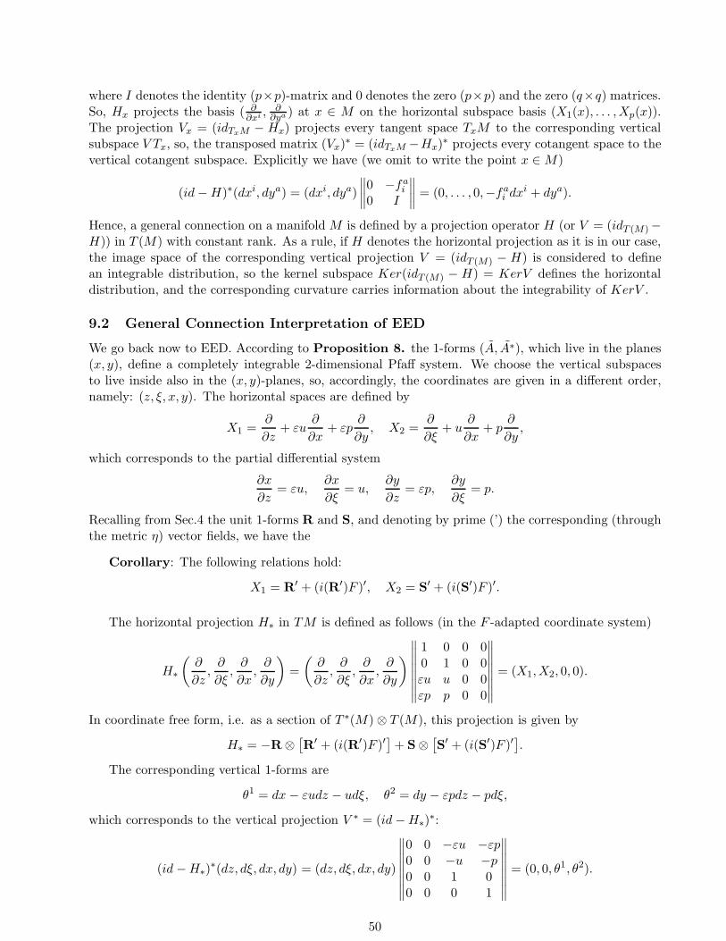
where I denotes the identity (p×p)-matrix and 0 denotes the zero (p×p) and the zero (q×q) matrices.So, Hx projects the basis ( ∂

∂xi ,∂

∂ya ) at x ∈ M on the horizontal subspace basis (X1(x), . . . ,Xp(x)).The projection Vx = (idTxM − Hx) projects every tangent space TxM to the corresponding verticalsubspace V Tx, so, the transposed matrix (Vx)∗ = (idTxM −Hx)

∗ projects every cotangent space to thevertical cotangent subspace. Explicitly we have (we omit to write the point x ∈M)

(id−H)∗(dxi, dya) = (dxi, dya)

∥∥∥∥0 −fa

i

0 I

∥∥∥∥ = (0, . . . , 0,−fai dx

i + dya).

Hence, a general connection on a manifold M is defined by a projection operator H (or V = (idT (M)−H)) in T (M) with constant rank. As a rule, if H denotes the horizontal projection as it is in our case,the image space of the corresponding vertical projection V = (idT (M) − H) is considered to definean integrable distribution, so the kernel subspace Ker(idT (M) − H) = KerV defines the horizontaldistribution, and the corresponding curvature carries information about the integrability of KerV .

9.2 General Connection Interpretation of EED

We go back now to EED. According to Proposition 8. the 1-forms (A, A∗), which live in the planes(x, y), define a completely integrable 2-dimensional Pfaff system. We choose the vertical subspacesto live inside also in the (x, y)-planes, so, accordingly, the coordinates are given in a different order,namely: (z, ξ, x, y). The horizontal spaces are defined by

X1 =∂

∂z+ εu

∂

∂x+ εp

∂

∂y, X2 =

∂

∂ξ+ u

∂

∂x+ p

∂

∂y,

which corresponds to the partial differential system

∂x

∂z= εu,

∂x

∂ξ= u,

∂y

∂z= εp,

∂y

∂ξ= p.

Recalling from Sec.4 the unit 1-forms R and S, and denoting by prime (’) the corresponding (throughthe metric η) vector fields, we have the

Corollary: The following relations hold:

X1 = R′ + (i(R′)F )′, X2 = S′ + (i(S′)F )′.

The horizontal projection H∗ in TM is defined as follows (in the F -adapted coordinate system)

H∗

(∂

∂z,∂

∂ξ,∂

∂x,∂

∂y

)=

(∂

∂z,∂

∂ξ,∂

∂x,∂

∂y

)∥∥∥∥∥∥∥∥

1 0 0 00 1 0 0εu u 0 0εp p 0 0

∥∥∥∥∥∥∥∥= (X1,X2, 0, 0).

In coordinate free form, i.e. as a section of T ∗(M) ⊗ T (M), this projection is given by

H∗ = −R⊗[R′ + (i(R′)F )′

]+ S⊗

[S′ + (i(S′)F )′

].

The corresponding vertical 1-forms are

θ1 = dx− εudz − udξ, θ2 = dy − εpdz − pdξ,

which corresponds to the vertical projection V ∗ = (id −H∗)∗:

(id −H∗)∗(dz, dξ, dx, dy) = (dz, dξ, dx, dy)

∥∥∥∥∥∥∥∥

0 0 −εu −εp0 0 −u −p0 0 1 00 0 0 1

∥∥∥∥∥∥∥∥= (0, 0, θ1, θ2).

50

Respectively, for the horizontal projection of the coordinate 1-forms we obtain

H∗(dz, dξ, dx, dy) =

∥∥∥∥∥∥∥∥

1 0 0 00 1 0 0εu u 0 0εp p 0 0

∥∥∥∥∥∥∥∥

dzdξdxdy

= (dz, dξ, εudz + udξ, εpdz + pdξ).

Recalling our isotropic 1-form ζ = εdz + dξ, we may write

H∗(dz) = dz, H∗(dξ) = dξ, H∗(dx) = dx− θ1 = u ζ, H∗(dy) = dy − θ2 = p ζ.

Making use of these relations we obtain

H∗dθ1 = ε(uξ − εuz)dz ∧ dξ, H∗dθ2 = ε(pξ − εpz)dz ∧ dξ.

Hence, for the curvature Ω, determined by the nonlinear solution F (u, p) we obtain

Ω(u, p) = ε(uξ − εuz)dz ∧ dξ ⊗∂

∂x+ ε(pξ − εpz)dz ∧ dξ ⊗

∂

∂y.

Corollary. The nonlinear solution F (u, p) is a running wave only if the curvature Ω(u, p) is equalto zero.

Denoting by η(X1) and η(X2) the η-corresponding 1-forms to X1 and X2, we compute the expres-sions < η(X1),Ω(u, p) > and < η(X2),Ω(u, p) >:

< η(X1),Ω(u, p) >=[ε(uξ − εuz) < η(X1),

∂

∂x> +ε(pξ − εpz) < η(X1),

∂

∂y>]dz ∧ dξ =

= −1

2

[(u2 + p2)ξ − ε(u2 + p2)z

]dz ∧ dξ = ε < η(X2),Ω(u, p) > .

So, relations < η(X1),Ω(u, p) >=< η(X2),Ω(u, p) >= 0 give equation (48).For the square of Ω we obtain

ΩσµνΩµν

σ = (uξ − εuz)2 + (pξ − εpz)

2 = φ2(ψξ − εψz)2, µ < ν.

Recalling now the formulas in Sec.5 we have

Corollary: The square of the tensor field Ω is equal to −(δF )2, so |Ω| = |δF |.

Corollary: A nonlinear solution may have rotational component of propagation only if the cur-vature form Ω is time-like, i.e. if Ω2 > 0.

In order to define the scale factor L in these terms we observe that the vertical components of thetwo coordinate vector fields ∂z and ∂ξ, given by

V∗ (∂z) = ∂z −H∗ (∂z) = ∂z −X1 = −εu ∂x − εp ∂y,

andV∗ (∂ξ) = ∂ξ −H∗ (∂ξ) = ∂ξ −X2 = −u∂x − p ∂y,

have the same modules equal to√u2 + p2. So, the scale factor L is given by

L =|V∗ (∂z)|

|Ω| =|V∗ (∂ξ)|

|Ω| .

51

Another way to introduce the scale factor only in terms of H∗ and Ω is the following. Recall thatthe space LW of linear maps in a linear space W is isomorphic to the tensor product W ∗⊗W , so, thespace LW ∗ of linear maps inW ∗ is isomorphic to W⊗W ∗. We shall define a map F : LW ×LW ∗ → LW .Let Φ ∈ LW and Ψ ∈ LW ∗ and ei and εj be two dual bases in W and W ∗ respectively. Then wehave the representations

Φ = Φjiε

i ⊗ ej , Ψ = Ψmn em ⊗ εn.

Now we define F(Φ,Ψ) as follows:

F(Φ,Ψ) = F(Φji ε

i ⊗ ej ,Ψmn em ⊗ εn) = Φj

iΨmn < εi, em > εn ⊗ ej = Φj

iΨinε

n ⊗ ej

For the composition tr F(Φ,Ψ) we obtain

tr F(Φ,Ψ) = ΦjiΨ

ij .

We compute now the matrix A of F(H∗, (id −H∗)∗) making use of the corresponding matrix repre-

sentations of these two linear maps given above.

A(F(H∗, (id−H∗)

∗))

=

∥∥∥∥∥∥∥∥

0 0 −εu −εp0 0 −u −p0 0 −2u2 −2up0 0 −2up −2p2

∥∥∥∥∥∥∥∥, tr(A) = −2(u2 + p2).

Hence, the relation Lζ(tr(A)) = 0 gives equation (48): (u2 + p2)ξ − ε(u2 + p2)z = 0, and we can definethe scale factor L as

L =

√12 |tr F(H∗, (id−H∗)∗)|

|Ω| .

On the other hand since L = |Lζψ|−1 (cf. relation (51)), where ψ is the phase of the solution, weobtain that ψ satisfies the differential equation

|Lζψ| =|Ω|√

12 |tr F(H∗, (id −H∗)∗)|

.

9.3 Principal Connection Interpretation

The principal connections are general connections on principal bundles [30] appropriately adaptedto the available bundle structure of the manifold. A principal bundle (P, π,B,G) consists of twomanifolds: the total space P and the base space B, a Lie group G, and a surjective smooth mapπ : P → B. There is a free smooth right action R : P × G → P of G on P, such, that the fibersπ−1(x), x ∈ B, are orbits Gx of G through x ∈ B, and every fiber Gx is diffeomorphic to G. Sincelocally P is diffeomorphic to Uα × G, where Uα ⊂ B is an open subset of B, the right action ofG on P is made appropriately consistent with the group product G × G → G, namely, there is acoordinate representation (Uα, ψα), where ψα : Uα × G → π−1(Uα) is a diffeomorphism such, thatR(ψα(x, a), b) = ψα(x, a).b = ψα(x, ab); a, b ∈ G.

If G is the Lie algebra of G then the right action R carries the elements h ∈ G to fundamental(vertical) vector fields Zh on P, and Zh, h ∈ G, define integrable distribution VG on P. So, choosingadditional to VG distribution H, we obtain a general connection on P. To make this general connectiona principal connection we make it consistent with the right action R of G on P in a natural way: thesubspace Hz.a at the point z.a ∈ P coincides with the image of Hz through (dRa)z, i.e. Hz.a =(dRa)z(Hz). The projection on the horizontal distribution is denoted by H∗.

The horizontal distribution can be defined by a connection form ω on P, which is G-valued 1-formand satisfies the conditions: ω(Zh) = h, h ∈ G; ω H∗ = 0 and R∗

aω = Ad(a−1) ω, a ∈ G. Then the

52

curvature Ω of the connection ω is given by Ω = dω H∗ = dω + 12 [ω, ω]. If the group is abelian, as

it is our case, then Ω = dω.If the bundle is trivial, i.e. P = M×G then the projection π is the projection on the first member:

π(x, a) = x, x ∈ M,a ∈ G. In this case with every connection form ω can be associated a G-valued1-form θ on the base space such, that ω(x, e;X,Zh) = h+ θ(x;X), where x ∈M,X ∈ TxM,h ∈ G ande is the identity of G [30, p.290]. For the curvature in the abelian case we obtain Ω = π∗dθ.

We go back now to EED. The base manifold of our trivial principal bundle P = M × G is, ofcourse, the Minkowski space-time M , and the abelian Lie group G is given by the (2×2)-real matrices

α(u, p) =

∥∥∥∥u p−p u

∥∥∥∥ , u2 + p2 6= 0.

The corresponding Lie algebra G, considered as a vecttor space, has the natural basis (I, J) and, asa set, it differs from G just by adding the zero (2 × 2)-matrix. According to the above, in order tointroduce a connection on P = M ×G it is sufficient to have a G-valued 1-form on M . We recall nowthat a nonlinear solution F in the F -adapted coordinate system defines the 1-form ζ = εdz + dξ andthe two functions (u, p). So, we define θ as

θ = uζ ⊗ I + pζ ⊗ J.

For the curvature we obtain

Ω = Ω1 ⊗ I + Ω2 ⊗ J = dθ =[uxdx ∧ ζ + uydy ∧ ζ − ε(uξ − εuz)dz ∧ dξ

]⊗ I

+[pxdx ∧ ζ + pydy ∧ ζ − ε(pξ − εpz)dz ∧ dξ

]⊗ J.

Since Ω is horizontal and, in our case, it is also G-invariant, there is just one G-valued 2-form Φ on Msuch, that π∗Φ = Ω. Further we identify Φ and Ω and write just Ω since in our coordinates they lookthe same. So, we can find ∗Ω with respect to the Minkowski metric in M :

∗Ω = (∗Ω1) ⊗ I + (∗Ω2) ⊗ J = ε[uxdy ∧ ζ − uydx ∧ ζ − ε(uξ − εuz)dx ∧ dy

]⊗ I

+ε[pxdy ∧ ζ − pydx ∧ ζ − ε(pξ − εpz)dx ∧ dy

]⊗ J.

We recall that the canonical conjugation α→ α∗ in G, given by (I, J) → (I,−J), defines the innerproduct in G by < α, β >= 1

2tr(α β∗). We have < I, I >= 1, < J, J >= 1, < I, J >= 0. We computethe expressions ∗ < Ω, ∗Ω >, < θ, ∗Ω >, ∧(θ, ∗Ω), and obtain respectively:

∗ < Ω, ∗Ω >= ∗(Ω1 ∧ ∗Ω1) < I, I > + ∗ (Ω2 ∧ ∗Ω2) < J, J >

= (uξ − εuz)2 + (pξ − εuz)

2 = −(δF )2.

< θ, ∗Ω >= −[u(uξ − εuz) + p(pξ − εpz)

]dx ∧ dy ∧ dz

−ε[u(uξ − εuz) + p(pξ − εpz)

]dx ∧ dy ∧ dξ,

∧(θ, ∗Ω) =[p(uξ − εuz) − u(pξ − εpz)

]dx ∧ dy ∧ dz

+ε[p(uξ − εuz) − u(pξ − εpz)

]dx ∧ dy ∧ dξ

⊗ I ∧ J = δF ∧ F ⊗ I ∧ J.

Corollary. Equations (18)-(20) are equivalent to the equation < θ, ∗Ω >= 0; a non-linear solutionmay have rotational component of propagation only if < Ω, ∗Ω > 6= 0; the equation d(δF ∧ F ) = 0 isequivalent to d

[∧ (θ, ∗Ω)

]= 0.

Since our principal bundle is trivial, the fundamental vector fields ZI and ZJ on M ×G, generatedby the basis vectors (I, J) in G coincide with the corresponding left invariant vector fields on G. Since

53

we have a linear group action, a left invariant vector field Zσ on G, at the point α ∈ G, generated byσ ∈ G is given by Zσ = (α,α σ). So, in our case, at the point

(x, β = (u, p)

)∈ M × G we obtain

ZI = uI + pJ ; ZJ = −pI + uJ . Hence, the metric on G gives |ZI | = |ZJ | =√u2 + p2. Therefore, for

the scale factor L we readily obtain

L =|ZI ||Ω| =

|ZJ ||Ω| .

Corollary: The 1-form θ, the curvature 2-form Ω and the scale factor L are invariant with respectto the group action (M × G,G) → (M × G).

Finally we note that we could write the 1-form θ in the form

θ = uζ ⊗ I + pζ ⊗ J = ζ ⊗ uI + ζ ⊗ pJ = ζ ⊗ ZI .

If we start with the new 1-form

θ′ = ζ ⊗ ZJ = ζ ⊗ (−pI) + ζ ⊗ (uJ) = −pζ ⊗ I + uζ ⊗ J

then, denoting dθ′ = Ω′, we obtain

∗ < Ω′, ∗Ω′ >= ∗ < Ω, ∗Ω >, < θ′, ∗Ω′ >= − < θ, ∗Ω >, ∧(θ′, ∗Ω′) = − ∧ (θ, ∗Ω).

Hence the last corollary and the definition of L stay in force with respect to θ′ too.

Remark. The group G acts on the right on the basis (I, J) of G. So, the transformed basis withβ(u, εp) ∈ G is Rβ(I, J) = (uI − εpJ, εpI + uJ). Now let ω be 1-form on M such that ω2 < 0 andω ∧ ∗ζ = 0. Then the corresponding generalized field is given by

Fω ⊗ I + ∗Fω ⊗ J == (ω ∧ ζ) ⊗ (uI − εpJ) + ∗(ω ∧ ζ) ⊗ (εpI + uJ).

In particular, ω = dx defines the field in an F -adapted coordinate system.

9.4 Linear connection interpretation

Linear connections ∇ are 1st-order differential operators in vector bundles. If such a connection ∇ isgiven and σ is a section of the bundle, then ∇σ is 1-form on the base space valued in the space ofsections of the vector bundle, so if X is a vector field on the base space then i(X)∇σ = ∇Xσ is a newsection of the same bundle. If f is a smooth function on the base space then ∇(fσ) = df ⊗ σ + f∇σ,which justifies the differential operator nature of ∇: the components of σ are differentiated and thebasis vectors are linearly transformed.

Let ea and εb, a, b = 1, 2, . . . , r be two dual local bases of the corresponding spaces of sections:< εb, ea >= δb

a, then we can write

σ = σaea, ∇ = d⊗ id+ Γbµadx

µ ⊗ (εa ⊗ eb), ∇(ea) = Γbµadx

µ ⊗ eb,

so∇(σmem) = dσm ⊗ em + σmΓb

µadxµ < εa, em > ⊗ eb =

[dσb + σaΓb

µadxµ]⊗ eb,

and Γbµa are the components of ∇ with respect to the coordinates xµ on the base space and with

respect to the bases ea and εb. Since the elements (εa ⊗ eb) define a basis of the space of (local)linear maps of the local sections, it becomes clear that in order to define locally a linear connection it

54

is sufficient to have some 1-form θ on the base space and a linear map φ = φbaε

a ⊗ eb in the space ofsections. Then

∇(σ) = dσa ⊗ ea + θ ⊗ φ(σ)

defines a linear connection with components Γbµa = θµφ

ba in these bases. So, locally, a linear connection

∇ may be written as∇ = d⊗ (εa ⊗ ea) + Ψb

µadxµ ⊗ (εa ⊗ eb).

If Ψ1 and Ψ2 are two such 1-forms then a map (Ψ1,Ψ2) → (∧,⊚)(Ψ1,Ψ2) is defined by (we shall writejust ⊚ for (∧,⊚) and the usual will mean just composition)

⊚(Ψ1,Ψ2) = (Ψ1)bµa(Ψ2)

nνmdx

µ ∧ dxν ⊗[ (εa ⊗ eb, ε

m ⊗ en)]

= (Ψ1)bµa(Ψ2)

nνmdx

µ ∧ dxν ⊗[< εa, en > (εm ⊗ eb)

]= (Ψ1)

bµa(Ψ2)

aνmdx

µ ∧ dxν ⊗ (εm ⊗ eb), µ < ν.

Now, in the case of trivial vector bundles, the curvature of ∇ is given by [30, p.328]

[d(Ψb

µadxµ)]⊗ (εa ⊗ ea) + ⊚(Ψ,Ψ).

We go back now to EED. The vector bundle under consideration is the (trivial) bundle Λ2(M) of2-forms on the Minkowski space-time M . From Section 7 we know that a representation ρ′ of G isdefined by relation (58). So, if α(u, p) ∈ G then ρ′(α) is a linear map in Λ2(M), and recalling our1-form ζ = εdz + dξ we define a linear connection ∇ in Λ2(M) by

∇ = d⊗ idΛ2(M) + ζ ⊗ ρ′(α(u, p)) = d ⊗ idΛ2(M) + ζ ⊗ (uI + pJ ), α ∈ G.

Two other connections ∇ and ∇∗ are defined by

ρ′(α(u, p)) = ρ′(α(u,−p)) = uI − pJ , and (ρ′)∗(α(u, p)) = ρ′(α.J) = ρ′(α(−p, u)) = −pI + uJ ,

and we shall denote:χ = uI + pJ , χ = uI − pJ , χ∗ = −pI + uJ .

So, we may say that χ represents F and χ∗ represents ∗F .Denoting Ψ = ζ ⊗ χ, Ψ = ζ ⊗ χ, Ψ∗ = ζ ⊗ χ∗, we note that (since ζ ∧ ζ = 0)

⊚(Ψ,Ψ) = ⊚(Ψ, Ψ) = ⊚(Ψ,Ψ∗) = 0.

Now, since Ψ = uζ⊗I+pζ⊗J , Ψ = uζ⊗I−pζ⊗J , Ψ∗ = −pζ⊗I+uζ⊗J for the correspondingcurvatures we obtain

R = d(uζ) ⊗ I + d(pζ) ⊗ J , R = d(uζ) ⊗ I − d(pζ) ⊗ J , R∗ = d(−pζ) ⊗ I + d(uζ) ⊗ J .

Remark. We have omitted here ε in front of pJ , but this is not essential since, putting p → εp inthe expressions obtained, we easily restore the desired generality.

By direct calculation we obtain:

∗1

6Tr[⊚(Ψ, ∗dΨ)

]= −ε

[u(uξ − εuz) + p(pξ − εpz)

]dz −

[u(uξ − εuz) + p(pξ − εpz)

]dξ;

1

6Tr [⊚(Ψ∗, ∗dΨ)] = ε

[p(uξ − εuz) − u(pξ − εpz)

]dx ∧ dy ∧ dz+

[p(uξ − εuz) − u(pξ − εpz)

]dx ∧ dy ∧ dξ = δF ∧ F ;

55

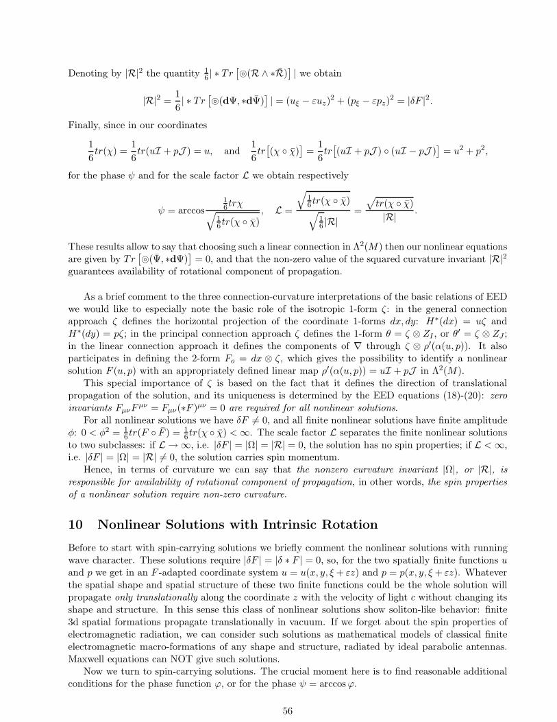
Denoting by |R|2 the quantity 16 | ∗ Tr

[⊚(R ∧ ∗R)

]| we obtain

|R|2 =1

6| ∗ Tr

[⊚(dΨ, ∗dΨ)

]| = (uξ − εuz)

2 + (pξ − εpz)2 = |δF |2.

Finally, since in our coordinates

1

6tr(χ) =

1

6tr(uI + pJ ) = u, and

1

6tr[(χ χ)

]=

1

6tr[(uI + pJ ) (uI − pJ )

]= u2 + p2,

for the phase ψ and for the scale factor L we obtain respectively

ψ = arccos16trχ√

16tr(χ χ)

, L =

√16tr(χ χ)√

16 |R|

=

√tr(χ χ)

|R| .

These results allow to say that choosing such a linear connection in Λ2(M) then our nonlinear equationsare given by Tr

[⊚(Ψ, ∗dΨ)

]= 0, and that the non-zero value of the squared curvature invariant |R|2

guarantees availability of rotational component of propagation.

As a brief comment to the three connection-curvature interpretations of the basic relations of EEDwe would like to especially note the basic role of the isotropic 1-form ζ: in the general connectionapproach ζ defines the horizontal projection of the coordinate 1-forms dx, dy: H∗(dx) = uζ andH∗(dy) = pζ; in the principal connection approach ζ defines the 1-form θ = ζ ⊗ ZI , or θ′ = ζ ⊗ ZJ ;in the linear connection approach it defines the components of ∇ through ζ ⊗ ρ′(α(u, p)). It alsoparticipates in defining the 2-form Fo = dx ⊗ ζ, which gives the possibility to identify a nonlinearsolution F (u, p) with an appropriately defined linear map ρ′(α(u, p)) = uI + pJ in Λ2(M).

This special importance of ζ is based on the fact that it defines the direction of translationalpropagation of the solution, and its uniqueness is determined by the EED equations (18)-(20): zeroinvariants FµνF

µν = Fµν(∗F )µν = 0 are required for all nonlinear solutions.For all nonlinear solutions we have δF 6= 0, and all finite nonlinear solutions have finite amplitude

φ: 0 < φ2 = 16tr(F F ) = 1

6tr(χ χ) <∞. The scale factor L separates the finite nonlinear solutionsto two subclasses: if L → ∞, i.e. |δF | = |Ω| = |R| = 0, the solution has no spin properties; if L <∞,i.e. |δF | = |Ω| = |R| 6= 0, the solution carries spin momentum.

Hence, in terms of curvature we can say that the nonzero curvature invariant |Ω|, or |R|, isresponsible for availability of rotational component of propagation, in other words, the spin propertiesof a nonlinear solution require non-zero curvature.

10 Nonlinear Solutions with Intrinsic Rotation

Before to start with spin-carrying solutions we briefly comment the nonlinear solutions with runningwave character. These solutions require |δF | = |δ ∗ F | = 0, so, for the two spatially finite functions uand p we get in an F -adapted coordinate system u = u(x, y, ξ+ εz) and p = p(x, y, ξ+ εz). Whateverthe spatial shape and spatial structure of these two finite functions could be the whole solution willpropagate only translationally along the coordinate z with the velocity of light c without changing itsshape and structure. In this sense this class of nonlinear solutions show soliton-like behavior: finite3d spatial formations propagate translationally in vacuum. If we forget about the spin properties ofelectromagnetic radiation, we can consider such solutions as mathematical models of classical finiteelectromagnetic macro-formations of any shape and structure, radiated by ideal parabolic antennas.Maxwell equations can NOT give such solutions.

Now we turn to spin-carrying solutions. The crucial moment here is to find reasonable additionalconditions for the phase function ϕ, or for the phase ψ = arccosϕ.

56

10.1 The Basic Example

The reasoning here follows the idea that these additional conditions have to express some internalconsistency among the various characteristics of the solution. A suggestion what kind of internalconsistency to use comes from the observation that the amplitude function φ is a first integral of thevector field ζ, i.e.

ζ(φ) =

(−ε ∂

∂z+

∂

∂ξ

)(φ) = −ε ∂

∂zφ(x, y, ξ + εz) +

∂

∂ξφ(x, y, ξ + εz) = 0.

In order to extend this consistency between ζ and φ we require the phase function ϕ to be first integralof some of the available F -generated vector fields. Explicitly, we require the following:

The phase function ϕ is a first integral of the three vector fields A,A∗ and S:

A(ϕ) = A∗(ϕ) = S(ϕ) = 0,

and the scale factor L is a first integral of R : R(L) = 0.

The first two requirements A(ϕ) = A∗(ϕ) = 0 define the following system of differential equationsfor ϕ:

−ϕ∂ϕ∂x

−√

1 − ϕ2∂ϕ

∂y= 0,

√1 − ϕ2

∂ϕ

∂x− ϕ

∂ϕ

∂y= 0.

Noticing that the matrix ∥∥∥∥∥−ϕ −

√1 − ϕ2√

1 − ϕ2 −ϕ

∥∥∥∥∥

has non-zero determinant, we conclude that the only solution of the above system is the zero-solution:

∂ϕ

∂x=∂ϕ

∂y= 0.

We conclude that in the coordinates used the phase function ϕ may depend only on (z, ξ). The thirdequation S(ϕ) = 0 requires ϕ not to depend on ξ in this coordinate system, so, ϕ = ϕ(z). For L weget

L =

√1 − ϕ2

|ϕz |.

Now, the last requirement, which in these coordinates reads

R(L) =∂L∂z

=∂

∂z

√1 − ϕ2

|ϕz |= 0,

means that the scale factor L is a pure constant: L = const. In this way the defining relation for Lturns into a differential equation for ϕ:

L =

√1 − ϕ2

|ϕz|→ ∂ϕ

∂z= ∓ 1

L√

1 − ϕ2. (74)

The obvious solution to this equation is

ϕ(z) = cos(κz

L + const), (75)

where κ = ±1. We note that the naturally arising in this case spatial periodicity 2πL and characteristicfrequency ν = c/2πL have nothing to do with the corresponding concepts in CED. In fact, the quantityL can not be defined in Maxwell’s theory.

57

The above considerations may be slightly extended and put in terms of the phase ψ, and in theseterms they look simpler. In fact, we have the equation

ψξ − εψz = κ1

L , κ = ±1,

where L = const. So, we get the two basic solutions

ψ1 = κz

L + const, ψ2 = κξ

L + const.

We get two kinds of periodicity: spatial periodicity along the coordinate z and time-periodicityalong the time coordinate ξ. The two values of κ = ±1 determine the two possible rotational structures:left-handed (left polarized), and right-handed (right polarized). Further we are going to concentrateon the spatial periodicity because it is strongly connected with the spatial shape of the solution. Inparticular, it suggests to localize the amplitude function φ inside a helical cylinder of height 2πL, so,the solution will propagate along the prolongation of this finite initial helical cylinder in such a waythat all points of the spatial support shall follow their own helical trajectories without crossings. Forsuch solutions with |δF | 6= 0 we are going to consider various ways for quantitative description ofthe available intrinsic rotational momentum, or the spin momentum, of these solutions. We call itspin-momentum by obvious reasons: it is of intrinsic nature and does not depend on any external pointor axis as it is the case of angular momentum. And it seems quite natural to follow the suggestionscoming from the corresponding considerations in Sec.5.

10.2 The G-Approach

In this first approach we make use of the corresponding scale factor L = const, of the isotropic 1-formζ and of the two objects ZI = uI + pJ and ZJ = −pI + uJ , considered as G-valued functions on M .By these quantities we build the following G ∧ G-valued 1-form H:

H = 2πκLcζ ⊗ (ZI ∧ ZJ). (76)

In components we have

Habµ = 2πκ

Lcζµ(Za

IZbJ − Zb

IZaJ).

In our system of coordinates we get

H = 2πκLcφ2 (εdz + dξ) ⊗ I ∧ J,

hence, the only non-zero components are

H123 = 2πκε

Lcφ2, H12

4 = 2πκLcφ2.

It is easily seen that ∗H is closed: d ∗H = 0. In fact,

d ∗H = 2πκLc

[(φ2)ξ− ε(φ2)z

](dx ∧ dy ∧ d ∧ dξ) ⊗ (I ∧ J) = 0

because φ2 is a running wave along the coordinate z. We restrict now ∗H to R3 and obtain

(∗H)R3 = 2πκLcφ2(dx ∧ dy ∧ dz) ⊗ (I ∧ J).

58

According to Stokes theorem, for finite solutions, we obtain the finite (conserved) quantity

H =

∫

R3

∗HR3 = 2πκLcE = κET I ∧ J,

which is a volume form in G, T = 2πL/c, and E is the integral energy of the solution. The module|H| of H is |H| = ET .

We see the basic role of the two features of the solutions: their spatially finite/concentratednature, giving finite value of all spatial integrals, and their translational-rotational dynamical naturewith |δF | 6= 0, allowing finite value of the scale factor L.

10.3 The FN-Bracket Approach

We proceed to the second approach to introduce spin-momentum. We recall the Froliher-Nijenhuisbracket SF of the finite nonlinear solution F , evaluated on the two unit vector fields A and εA∗:

(SF )σµνAµεA∗ν = (SF )σ12(A

1εA∗2 − A2εA∗1).

For (SF )σ12 we get

(SF )112 = (SF )212 = 0, (SF )312 = −ε(SF )412 = 2εp(uξ − εuz) − u(pξ − εpz).

It is easily seen that the following relation holds: A1εA∗2−A2εA∗1 = 1. Now, for the above obtainedsolution for ϕ we have

u = φ(x, y, ξ + εz) cos(κz

L + const), p = φ(x, y, ξ + εz) sin

(κz

L + const).

We obtain(SF )312 = −ε(SF )412 = −2ε

κ

Lφ2,

(SF )σµνAµεA∗ν =

[0, 0,−2ε

κ

Lφ2, 2

κ

Lφ2].

Since φ2 is a running wave along the z-coordinate, the vector field SF (A, εA∗) has zero divergence:∇ν [SF (A, εA∗)]ν = 0. Now, defining the helicity vector of the solution F by

ΣF =L2

2cSF (A, εA∗),

then ΣF has also zero divergence, and the integral quantity∫

(ΣF )4dxdydz

does not depend on time and is equal to κET .

10.4 The d(F ∧ δF ) = 0 Approach

Here we make use of the equation d(F ∧ δF ) = 0 and see what restrictions this equation imposes onψ. In our system of coordinates this equation is reduced to

d(F ∧ δF ) = εΦ2 (ψξξ + ψzz − 2εψzξ) dx ∧ dy ∧ dz ∧ dξ = 0, (77)

i.e.ψξξ + ψzz − 2εψzξ = (ψξ − εψz)ξ − ε (ψξ − εψz)z = 0. (78)

Equation (78) has the following solutions:

59

1o. Running wave solutions ψ = ψ(x, y, ξ + εz),2o. ψ = ξ.g(x, y, ξ + εz) + b(x, y),3o. ψ = z.g(x, y, ξ + εz) + b(x.y),4o. Any linear combination of the above solutions with coefficients which are allowed to depend

on (x, y).The functions g(x, y, ξ + εz) and b(x, y) are arbitrary in the above expressions.

The running wave solutions ψ1, defined by 1o, lead to F ∧ δF = 0 and to |δF | = 0, and by thisreason they have to be ignored. The solutions ψ2 and ψ3, defined respectively by 2o and 3o, give thescale factors L = 1/|g|, and since L is dually invariant it should not depend on (x, y) in this coordinatesystem. Hence, we obtain g = g(ξ + εz), so, the most natural choice seems g = const, which impliesalso L = const. A possible dependence of ψ on (x, y) may come only through b(x, y). Note that thephysical dimension of L is length and b(x, y) is dimensionless.

We turn now to the integral spin-momentum computation. In this approach its density is givenby the correspondingly normalized 3-form F ∧ δF . So we normalize it as follows:

β = 2πL2

cF ∧ δF = 2π

L2

c

[−εφ2(ψξ − εψz)dx ∧ dy ∧ dz − φ2(ψξ − εψz)dx ∧ dy ∧ dξ

]. (79)

The physical dimension of β is ”energy-density × time”. We see that β is closed: dβ = 0, so we mayuse the Stokes’ theorem. The restriction of β to R

3 is:

βR3 = 2πL2

c

[−εφ2(ψξ − εψz)dx ∧ dy ∧ dz

].

Let’s consider first the solutions 3o of equation (78) with L = const. The corresponding phaseψ = κ z

L+ b(x, y), κ = ±1, requires spatial periodicity of 2πL along the coordinate z. So, if we

restrict the spatial extension of the solution along z to one such period lo = 2πL, our solutionwill occupy at every moment a one-step part of a helical (screw) cylinder. Its time evolution willbe a translational-rotational propagation along this helical cylinder. So, we have an example of anobject with helical spatial structure and with intrinsical rotational component of propagation, andthis rotational component of propagation does NOT come from a rotation of the object as a wholearound some axis.

On the contrary, the solutions defined by 2o, are NOT obliged to have spatial periodicity. Theirevolution includes z-translation and rotation around the z-axis as a whole together with some rotationaround themselves.

For the case 3o with L = const we can integrate

βR3 =2πLcκφ2dx ∧ dy ∧ dz

over the 3-space and obtain ∫

R3

β = κE2πLc

= κET = ±ET, (80)

where E is the integral energy of the solution, T = 2πL/c is the intrinsically defined time-period,and κ = ±1 accounts for the two polarizations. According to our interpretation this is the integralspin-momentum of the solution for one period T .

10.5 The Nonintegrability Approach

Here we make use of the observation that the two Pfaff systems (A, ζ) and (A∗, ζ) are nonintegrablewhen L 6= 0. From Sec.5 we have

dA ∧ A ∧ ζ = dA∗ ∧ A∗ ∧ ζ = ε[u(pξ − εpz) − p(uξ − εuz)

]dx ∧ dy ∧ dz ∧ dξ

= εφ2(ψξ − εψz)dx ∧ dy ∧ dz ∧ dξ.

60

Integrating the 4-form2πεLc

dA ∧ A ∧ ζ

on the 4-volume R3 × L we obtain κET .

We recall also that for finite solutions the electromagnetic volume form ωχ = −1cA ∧ ˜εA∗ ∧ R ∧ S

gives the same quantity ET when integrated over the 4-volume R3 × L, L = const.

10.6 The Godbillon-Vey 3-form as a Conservative Quantity

According to the Frobenius integrability theorems having a completely integrable (n− 1)-dimensionaldifferential system on a n-manifold M is equivalent to having a suitable completely integrable 1-dimensional Pfaff system on the same manifold. This Pfaff system is determined by a suitable 1-formω, defined up to a nonvanishing function: fω, f(x) 6= 0, x ∈M , and ω satisfies the equation dω∧ω = 0(so obviously, fω also satisfies d(fω)∧ fω = 0). From this last equation it follows that there is 1-formθ such, that dω = θ ∧ ω. Now, the Godbillon-Vey theorem [31] says that the 3-form β = dθ ∧ θ isclosed: dβ = d(dθ ∧ θ) = 0, and, varying θ and ω in an admissible way: θ → (θ+ gω); ω → fω, leadsto adding an exact 3-form to β, so we have a cohomological class Γ defined entirely by the integrable 1-dimensional Pfaff system. From physical point of view the conclusion is that each completely integrable1-dimensional Pfaff system on Minkowski space generates a conservation law through the restrictionof β on R

3.Recall now the following objects on our Minkowski space-time: A, A∗ and ζ. These are 1-forms.

We form the corresponding vector fields through the Lorentz-metric and denote them by ~A, ~A∗, ~ζ.Let’s consider the 1-form ω = fζ = εfdz + fdξ, where f is a nonvanishing function on M . We havethe relations:

ω( ~A) = 0, ω( ~A∗) = 0, ω(~ζ) = 0.

Moreover, since ζ is closed, ω = fζ satisfies the Frobenius integrability condition:

dω ∧ ω = fdf ∧ ζ ∧ ζ = 0.

Therefore, the corresponding 1-dimensional Pfaff system, defined by ω = fζ, is completely integrable,and there exists a new 1-form θ, such that dω = θ ∧ ω, and d(dθ ∧ θ) = 0.

From the point of view of generating a conservative quantity through integrating the restrictioni∗β of β = dθ∧θ to R

3, through the imbedding i : (x, y, z) → (x, y, z, 0) it is not so important whetherΓ is trivial or nontrivial. The important point is the 3-form β to have appropriate component β123

in front of the basis element dx ∧ dy ∧ dz, because only this component survives after the restrictionconsidered is performed, which formally means that we put dξ = 0 in β. The value of the correspondingconservative quantity will be found provided the integration can be carried out successfully, i.e. when(i∗β)123 has no singularities and (i∗β)123 is concentrated in a finite 3d subregion of R

3.In order to find appropriate θ in our case we are going to take advantage of the freedom we have

when choosing θ: the 1-form θ is defined up to adding to it an 1-form γ = g ω, where g is an arbitraryfunction on M , because θ is defined by the relation dω = θ∧ω, and (θ+ g ω)∧ω = θ∧ω always. Thefreedom in choosing ω consists in choosing the function f , and we shall show that f may be chosen insuch a way: ω = f ζ, that the corresponding integral of i∗β to present a finite conservative quantity.

Recalling that dζ = 0, we have

dω = d(fζ) = df ∧ ζ + fdζ = df ∧ ζ.

Since dω must be equal to θ ∧ ω we obtain

dω = df ∧ ζ = θ ∧ ω = θ ∧ (fζ) = fθ ∧ ζ.

61

It follows

θ ∧ ζ =1

fdf ∧ ζ = d(ln f) ∧ ζ =

[d(ln f) + hζ

]∧ ζ,

where h is an arbitrary function. Hence, in general, we obtain θ = d(ln f) + hζ. Therefore, sincedθ = dh ∧ ζ for dθ ∧ θ we obtain

dθ ∧ θ = d(ln f) ∧ dh ∧ ζ.

Denoting for convenience (ln f) = ϕ for the restriction i∗β we obtain

i∗β = ε(ϕxhy − ϕyhx)dx ∧ dy ∧ dz.

In order to find appropriate interpretation of i∗β we recall that ∗(δF ∧F ) = −εφ2(ψξ − εψz)ζ, so,∗(δF ∧F ) is of the kind f ζ, and it defines the same 1-dimensional Pfaff system as f ζ does. We recallalso that if the scale factor L = 1/|ψξ −εψz| is a nonzero constant then φ2(ψξ −εψz) is a running waveand the 3-form δF ∧F is closed. Hence, the interpretation of i∗β as i∗(δF ∧F ) = − 1

Lεκφ2dx∧dy∧dz

requires appropriate definition of the two functions f and h. So we must have

ϕxhy − hxϕy = −κ

Lφ2.

If we choose

f = exp(ϕ) = exp

[∫φ2dx

], h = −κ

Ly + const

all requirements will be fulfilled, in particular, ϕxy = ϕyx = (φ2)y and hxy = hyx = 0.Hence, the above choice of f and h allows the spatial restriction of the Godbillon-Vey 3-form β to

be interpreted as the spatial restriction of F ∧ δF . So, the curvature expressions found in the previoussections, as well as the corresponding spin-properties of the nonlinear solutions being available whenδF ∧ F 6= 0, are being connected with the integrability of the Pfaff system ω = f ζ.

On the two figures below are given two theoretical examples with κ = −1 and κ = 1 respectively,amplitude function φ located inside a one-step helical cylinder with height of 2πL, and phase functionϕ = cos(κz/L). The solutions propagate left-to-right along the coordinate z.

Figure 1: Theoretical example with κ = −1. The Poynting vector is directed left-to-right.

Figure 2: Theoretical example with κ = 1. The Poynting vector is directed left-to-right.

62

In the case κ = −1 the magnetic vector is always directed to the rotation axis, i.e. it is normalto the rotation, and the electric vector is always tangent to the rotation, so, looking from behind (i.e.along the Poynting vector) we find clock-wise rotation. In the case κ = 1 the two vectors exchangetheir roles and, looking from behind again, we find anti-clock-wise rotation. From structural point ofview the case κ = −1 is obtained from the case κ = 1 through rotating the couple (E,B) anti-clock-wise to the angle of π/2, hence we get the (dual) transformation (E,B) → (−B,E). The dynamicalroles of the two vectors are exchanged: now the electric vector drags the points of the object towardsrotation axis, the magnetic vector generates rotation. In both cases the Poynting vector ”pushes” theobject along the rotation axis.

The above pictures suggest the interpretation that the rotation axis directed vectors keep the objectfrom falling apart, and such kind of dynamical structure seems to be the only possible time-stableone.

If we project the object on the plane orthogonal to the Poynting vector we shall obtain a sectorbetween two circles with the same center, and this sector has nontrivial topology. One of the twovectors is always directed to the center of the circles and this stabalizes the solution, and the other istangent to the circles and correspondingly oriented. The stability of the construction is in accordancealso with the fact that, when z runs from zero to 2πL any of the two vectors performs just one fullrotation. Any other rotaional evolution would make the center-directed vector leave its directional be-havior and this would bring to structural changes and, most probably, to falling apart of the structure.Choosing orientation and computing the corresponding rotation numbers of E and B we shall obtain,depending on the orientation chosen, (+1), or (−1), and in definite sense these values guarantee frommathematical viewpoint the dynamical stability of the solution-object.

11 Explicit Non-vacuum Solutions

Before to start searching solutions with nonzero αi, i = 1, 2, 3, 4, we must keep in mind that the fieldF now will certainly be of quite different nature compare to the vacuum case, and its interpretationas electromagnetic field is much conditional: no more propagation with the Lorentz invariant speed,no more photon-likeness, etc. The solution is meant to represent a field interacting continuouslywith other physical system, so the situation is quite different and, correspondingly, the properties ofthe solution may differ drastically from the vacuum solutions properties. For example, contrary tothe nonlinear vacuum case where the solutions propagate translationally with the velocity of light,here it is not excluded to find solutions which do not propagate with respect to an appropriateLorentz frame. In integrability-nonintegrability terms this would mean that at least some of theproper integrability properties of the vacuum solutions have been lost. On the other hand, the properintegrability properties of the external field are, at least partially, guaranteed to hold through therequirement for the Frobenius integrability of the 2-dimensional Pfaff systems (αi, αj).

As a first step we expect possible physical interpretation just in the frame of macro phenomena,where the continuity of the energy-momentum exchange is easily understood, but we do not excludeinterpretations in the frame of microworld in view of the large quantity of variables we have (in fact, 22functions), and in view of the universality of the physical process described, namely, energy-momentumexchange.

From purely formal point of view finding a solution, whatever it is, legitimizes the equations con-sidered as a consistent system. Our purpose in looking for solutions in the nonvacuum case, however,is not purely formal, we’d like to consider the corresponding solutions as physically meaningful, inother words, we are interested in solutions, which can be, more or less, physically interpretable, i.e.presenting more or less approximate models of real objects and processes. That’s why we’ll try to meetthe following. First, the solutions must be somehow physically clear, which means that the anzatzassumed should be comparatively simple and its choice should be made on the base of a preliminaryanalysis of the physical situation in view of the mathematical model used. Second, it is absolutely

63

obligatory the solutions to have well defined local and integral energy and momentum. Third, thesolutions are desirable to be in the spirit of the soliton-like consideration of the real natural objectswhen a corresponding physical interpretation is meant to be done. Finally, it would be nice, the solu-tions found to be comparatively simple and to have something to do with ”popular” and well knownsolutions of ”well liked” equations.

11.1 Choice of the anzatz and finding the solutions

Let’s now get started. We shall be interested in time-dependent solutions, therefore, the ”electric”and the ”magnetic” components should present. The simplest (F, ∗F ), meeting this requirement, lookas follows (we use the above assumed notations):

F = −udy ∧ dz − vdy ∧ dξ, ∗F = vdx ∧ dz + udx ∧ dξ, (81)

where u and v are two functions on M . Second, when choosing the 1-forms αi we shall follow therequirement, that the ”medium” does not influence the F ↔ ∗F exchange, so we put

α2 = α3 = 0. (82)

Third, since the rest two 1-forms , α1 and α4 must be linearly independent (they must define a 2-dimensional Pfaff system), we choose them to be mutually orthogonal and let α4 be time-like, and theother to be space-like. The simplest time-like 1-form looks like α = A(x, y, z, ξ)dξ, moreover, any such1-form defines integrable 1-dimensional Pfaff system:

dα ∧ α = (Axdx ∧ dξ +Aydy ∧ dξ +Azdz ∧ dξ) ∧Adξ = 0.

So, we choose α4 = A(x, y, z, ξ)dξ. Finally, for α1, denoted further by β, we obtain in general,β = β1dx + β2dy + β3dz. Clearly, β2 < 0, and α.β = 0, so they are linearly independent. Now, βparticipates in the equations through the expression β ∧ ∗F , and from the explicit form of ∗F is seen,that the coefficient β1 in front of dx does not take part in β∧∗F , therefore, we put β1 = 0. So, puttingβ2 = b and β3 = −B for convenience, we get

α1 ≡ β = bdy −Bdz, α4 ≡ α = Adξ, α2 = α3 = 0. (83)

We note, that the so chosen β does not define in general an integrable 1-dimensional Pfaff system, so,accordingly: dα ∧ α = 0, dβ ∧ β 6= 0.

At these conditions our equations

δ ∗ F ∧ F = α ∧ F, δF ∧ ∗F = β ∧ ∗F, δ ∗ F ∧ ∗F − δF ∧ F = 0,

dα ∧ α ∧ β = 0, dβ ∧ α ∧ β = 0

take the form: δ ∗ F ∧ ∗F − δF ∧ F = 0 is reduced to

−vuy + uvy = 0, −uvx + vux = 0,

the Frobenius equations dα ∧ α ∧ β = 0, dβ ∧ α ∧ β = 0 reduce to

(−bxB +Bxb) .A = 0,

δ ∗ F ∧ F = α ∧ F is reduced to

u (uξ − vz) = 0, v (uξ − vz) = 0, uux − vvx = Au,

64

finally, δF ∧ ∗F = β ∧ ∗F reduces to

v (vξ − uz) = −bv, u (vξ − uz) = −bu, uuy − vvy = Bu.

In this way we obtain 7 equations for 5 unknown functions u, v,A,B, b.The equations −vuy + uvy = 0, −uvx + vux = 0 have the following solution:

u(x, y, z, ξ) = f(x, y)U(z, ξ), v(x, y, z, ξ) = f(x, y)V (z, ξ).

That’s why

AU = fx

(U2 − V 2

), BU = fy

(U2 − V 2

), f (Vξ − Uz) = −b, Uξ − Vz = 0.

It follows that b should be of the kind b(x, y, z, ξ) = f(x, y)bo(z, ξ), so the equation Bxb − Bbx = 0takes the form

ffxy = fxfy.

The general solution of this last equation is f(x, y) = g(x)h(y). The equation gh (Vξ − Uz) = −breduces to

Vξ − Uz = −bo.The relations obtained show how to build a solution of this class. Namely, first, we choose the

function V (z, ξ), then we determine the function U(z, ξ) by

U(z, ξ) =

∫Vzdξ + l(z),

where l(z) is an arbitrary function, which may be assumed equal to 0. After that we define bo = Uz−Vξ.The functions g(x) and h(y) are arbitrary, and for A and B we find

A(x, y, z, ξ) = g′(x)h(y)U2 − V 2

U, B(x, y, z, ξ) = g(x)h′(y)

U2 − V 2

U.

In this way we obtain a family of solutions, which is parametrized by one function V of the twovariables (z, ξ) and two functions g(x), h(y), each depending on one variable.

In order to find corresponding conserved quantities we sum up the nonzero right-hand sides of theequations and obtain ∗(α∧F +β ∧∗F ). We represent this expression in a divergence form as follows:

∗(α ∧ F + β ∧ ∗F ) = Audx−Budy − budz − bvdξ =

=1

2(U2 − V 2)

[(gh)2

]xdx− 1

2(U2 − V 2)

[(gh)2

]ydy−

−(gh)2(∫

Ubodz

)

z

dz − (gh)2(∫

V bodξ

)

ξ

dξ == −

∂

∂xνP ν

µ

dxν ,

where the interaction energy-momentum tensor is defined by the matrix

P νµ =

∥∥∥∥∥∥∥∥

−12(gh)2Z 0 0 0

0 12(gh)2Z 0 0

0 0 (gh)2∫Ubodz 0

0 0 0 (gh)2∫V bodξ

∥∥∥∥∥∥∥∥,

and the notation Z ≡ U2 − V 2 is used. For the components of the full energy tensor T νµ = Qν

µ + P νµ

we obtain

T 33 = (gh)2

[∫Ubodz − 1

2(U2 + V 2)

],

T 43 = −T 3

4 = (gh)2UV,

T 44 = (gh)2

[∫V bodξ +

1

2(U2 + V 2)

],

and all other components are zero.

65

11.2 Examples

In this subsection we consider some of the well known and well studied (1+1)-dimensional solitonequations as generating procedures for choosing the function V (z, ξ), and only the 1-soliton solutionswill be explicitly elaborated. Of course, there is no anything standing in our way to consider other(e.g. multisoliton) solutions. We do not give the corresponding formulas just for the sake of simplicity.

We turn to the soliton equations mainly because of two reasons. First, most of the solutions havea clear physical sense in a definite part of physics and, according to our opinion, they are sufficientlyattractive for models of real physical objects with internal structure. Second, the soliton solutionsdescribe free and interacting objects with no dissipation of energy and momentum, which correspondsto our understanding of the Frobenius integrability equations as criteria for availability of integralproperties of the medium considered.

1. Nonlinear (1+1) Klein-Gordon Equation. In this example we define our functions U and V throughthe derivatives of the function k(z, ξ) in the following way: U = kz, V = kξ. Then the equationUξ − Vz = kzξ − kξz = 0 is satisfied automatically, and the equation Uz − Vξ = bo takes the formkzz − kξξ = bo. Since bo is unknown, we may assume bo = bo(k), which reduces the whole problem tosolving the general nonlinear Klein-Gordon equation when bo depends nonlinearly on k. Since in thiscase V = kξ we have

∫V bo(k)dξ =

∫kξb

o(k)dξ =

∫ [∂

∂ξ

∫bo(k)dk

]dξ =

∫bo(k)dk.

For the full energy density we get

T 44 =

1

2(gh)2

k2

z + k2ξ + 2

∫bo(k)dk

.

Choosing bo(k) = m2sin(k), m = const, we get the well known and widely used in physics Sine-Gordonequation, and accordingly, we can use all solutions of this (1+1)-dimensional nonlinear equation togenerate (3+1)-dimensional solutions of our equations following the above described procedure. Whenwe consider the (3+1) extension of the soliton solutions of this equation, the functions g(x) and h(y)should be localized too. The determination of the all 5 functions in our approach is straightforward,so we obtain a (3+1)-dimensional version of the soliton solution chosen. As it is seen from the abovegiven formulas, the integral energy of the solution differs from the energy of the corresponding (1+1)-dimensional solution just by the (x, y)-localizing factor [g(x)h(y)]2.

For the 1-soliton solution (kink) we have:

k(z, ξ) = 4arctg

exp

[±mγ

(z − w

cξ)

], γ =

√1 − w2

c2

U(z, ξ) = kz =±2m

γch[±m

γ

(z − w

cξ)] , V (z, ξ) = kξ =

±2mw

cγch[±m

γ

(z − w

cξ)] ,

A = g′(x)h(y)±2mγ

ch[±m

γ

(z − w

cξ)] , B = g(x)h′(y)

±2mγ

ch[±m

γ

(z − w

cξ)] ,

bo = Uz − Vξ =−2m2sh

[±m

γ

(z − w

cξ)]

ch[±m

γ

(z − w

cξ)] , T 4

4 =(gh)24m2

γ2ch2[±m

γ

(z − w

cξ)]

and for the 2-form F we get

F = − ±2mg(x)h(y)

γch[±m

γ(z − w

cξ)]dy ∧ dz +

w

c

±2mg(x)h(y)

γch[±m

γ(z − w

cξ)]dy ∧ dξ.

66

In its own frame of reference this soliton looks like

F = −±2mg(x)h(y)

ch(±mz) dy ∧ dz.

From this last expression and from symmetry considerations, i.e. at homogeneous and isotropicmedium, we come to the most natural (but not necessary) choice of the functions g(x) and h(y):

g(x) =1

ch(mx), h(y) =

1

ch(my).

2.Korteweg-de Vries equation. This nonlinear equation has the following general form:

fξ + a1ffz + a2fzzz = 0,

where a1 and a2 are 2 constants. The well known 1-soliton solution is

f(z, ξ) =ao

ch2[

zL− w

cLξ] , L = 2

√3a2

aoa1, w =

caoa1

3,

where ao is a constant. We choose V (z, ξ) = f(z, ξ) and get

U = −aoc

w

1

ch2[

zL− w

cLξ] , bo = Uz − Vξ =

( c

Lw− w

c

) 2ao

ch3[

zL− w

cLξ] ,

T 44 = (gh)2

a2oc

2(1 + L)

2w2Lch4[

zL− w

cLξ] .

3. Nonlinear Schrodinger equation. In this case we have an equation for a complex-valued function,i.e. for two real valued functions. The equation reads

ifξ + fzz + |f |2f = 0,

and its 1-soliton solution, having oscillatory character, is

f(z, ξ) = 2β2 exp[−i(2αz + 4(α2 − β2)ξ − θ

)]

ch (2βz + 8αβξ − δ),

where α, β, δ and θ are constants. The natural substitution f(z, ξ) =√ρ.exp(iϕ) brings this equation

to the following two equations

ρξ + (2ρϕz)z = 0, 4ρ+2ρρzz − ρ2

z

ρ2= 4(ϕξ + ϕ2

z).

For the 1-soliton solution we get

ρ =4β4

ch2 (2βz + 8αβξ − δ), ϕ = −

[2αz + 4(α2 − β2)ξ − θ

].

We put U = ρ, V = −2ρϕz and obtain

U = ρ =4β4

ch2 (2βz + 8αβξ − δ), V = −2ρϕz =

16αβ4

ch2 (2βz + 8αβξ − δ),

A = g′(x)h(y)4β4(1 − 16α2)

ch2 (2βz + 8αβξ − δ), B = g(x)h′(y)

4β4(1 − 16α2)

ch2 (2βz + 8αβξ − δ),

67

bo =16β3(16α2β2 − 1)sh(2βz + 8αβξ − δ)

ch3(2βz + 8αβξ − δ),

T 44 = (gh)2

16β8

ch4(2βz + 8αβξ − δ).

We note that the solution of our equations obtained has no the oscillatory character of the originalSchrodinger 1-soliton solution, it is a (3+1)-localized running wave and moves as a whole with thevelocity 4cα, so in the relativistic frame we must require 4cα < c.

4.Boomerons. The system of differential equations, having soliton solutions, known as boomerons,is defined by the following functions: K : R2 → R3, H : R2 → R, and besides, two constant3-dimensional vectors r and s, where s is a unit vector: |s| = 1. The equations have the form

Hξ − s.Kz = 0, Kzξ = Hzzs + r× Kz − 2Kz × (K × s).

Now we have to define our functions U(z, ξ), V (z, ξ) and bo(z, ξ). The defining relations are:

U = Hz = |s|2Hz, V = s.Kz = (s.K)z , bo = −s. [r ×Kz − 2Kz × (K × s)] .

Under these definitions our equations Uξ − Vz = 0, Vξ − Uz = −bo look as follows:

[Hz − s.Kz ]z = 0, s. [Kzξ −Hzzs − r× Kz + 2Kz × (K × s)] = 0.

It is clear that every solution of the ”boomeron” system determines a solution of our system ofequations according to the above given rules and with the multiplicative factors g(x) and h(y). Thetwo our functions A(z, ξ) and B(z, ξ) are easily then computed.

Following this procedure we can generate a spatial soliton solution to our system of equations bymeans of every solution, in particular every soliton solution, to any (1+1)-soliton equation, as well as tocompute the corresponding conserved quantities. It seems senseless to give here these easily obtainableresults. The richness of this comparatively simple family of solutions, as well as the availability ofcorresponding correctly defined integral conserved quantities, are obvious and should not be neglectedas a generating procedure for obtaining (3+1) one-soliton, as well as, (3+1) many-soliton solutions.

68

12 Retrospect and Outlook

In trying to understand our observational knowledge of the real world we must be able to separate theimportant structural and behavioral properties of the real objects from those, the changes of whichduring time-evolution do not lead to annihilation of the objects under consideration. One of the basicin our view lessons that we more or less have been taught is that the physical objects are spatially finiteentities, and that for their detection and further study some energy-momentum exchange is necessarilyrequired. So, every physical object necessarily carries energy-momentum and every interaction betweentwo physical objects has such an energy-momentum exchange aspect. The second lesson concerningany interaction is that, beyond its universality, energy-momentum is a conserved quantity, so NO lossof it is allowed: it may only pass from one object to another. This means that every annihilationprocess causes creation process(es), and the full energy-momentum that has been carried by theannihilated objects, is carried away by the created ones. Energy-momentum always needs carriers,as well as every physical object always carries energy-momentum. Hence, the energy-momentumexchange abilities of any physical object realize its protection against external influence on one side,and reveal its intrinsic nature, on the other side. Therefore, our knowledge about the entire complexof properties of a physical object relies on getting information about its abilities in this respect andfinding corresponding quantities describing quantitatively these abilities.

The spatially finite nature of a physical object implies spatial structure and finite quantity ofenergy-momentum needed for its creation, so NO structureless and infinite objects may exist. Theapproximations for ”point object” and ”infinite field”, although useful in some respects, seem the-oretically inadequate and should not be considered as basic ones. More reliable appears to be theapproximation ”finite continuous object”, which we tried to follow throughout our exposition. Thislast approximation suggests that nonlinear partial differential equations should be the basic tool forbuilding mathematical models of local nature of such objects. The natural physical sense of theseequations is naturally supposed to be local energy-momentum exchange.

Another useful observation is that physical objects are many-aspect entities, they have complicatedstructure and their very existence is connected with internal energy-momentum exchange/redistributionamong the various structural components. So, the mathematical model objects should be many-component ones, and with appropriate mathematical structure. Of basic help in finding appropriatemathematical objects is having knowledge of the internal symmetry properties of the physical objectunder consideration. This ”step by step” process of getting and accumulating important informationabout the physical properties of natural objects reflects in the ”step by step” process of refining thecorresponding mathematical models.

The greatest discovery at the very beginning of the last century was that the notion of electro-magnetic field as suggested by Maxwell equations is inadequate: the time dependent electromagneticfield is not an infinite smooth perturbation of the aether, on the contrary, it consists of many individ-ual time-stable objects, called later photons, which are created/destroyed mainly during intra-atomicenergy-transition processes. Photons are finite objects, they carry energy-momentum and after theyhave been radiated outside their atom-creator, they propagate as a whole translationally by the speedof light. Moreover, their propagation is not just translational, it includes rotational component, whichis of intrinsic and periodical nature. The corresponding intrinsic action for one period T is h = ET ,where E is the full energy of the photon, and all photons carry the same intrinsic action h. Duringthe entire 20th century physicists have tried to understand the dynamical structure/nature of photonsfrom various points of view, and this process is still going on today.

Extended Electrodynamics, as presented in the preceding sections, is an attempt in this direc-tion. The basic starting observation for approaching the problem is that the energy-momentum localquantities and relations of Maxwell theory do agree with the experiment, but the free field equationsδF = 0, δ ∗ F = 0 give non-realistic free time-dependent solutions: they are either strongly time-unstable, or infinite. Hence, these solutions can not be used as mathematical models of photons, since

69

the latter are time-stable and finite objects. The basic idea of writing down new nonlinear equa-tions was to pass to local energy-momentum relations, describing how the internal energy-momentumexchanges are carried out. The mathematical structure of Maxwell equations and local conserva-tion relations allowed the extension procedure to be used, so the new nonlinear equations contain allMaxwell solutions as exact solutions. This feature is important from the point of view of applications.

In order to come to the new equations we made use of the dual symmetry of the linear solutions,which suggested to consider the field as having two vector components (F, ∗F ), and introduced theconcept of G-covariant Lorentz force as a natural generalization of the known Lorentz force. The G-covariant Lorentz force has three vector components, and each component has a clear physical senseof corresponding local energy-momentum change, as it should be. The two components FµνδF

ν and(∗F )µν(δ ∗ F )ν determine how much energy-momentum the field is potentially able to give out tosome other physical object through any of the two components F and ∗F , and the third componentFµν(δ ∗ F )ν + (∗F )µνδF

ν characterizes the internal energy-momentum exchange between the twocomponents F and ∗F . We concluded that in case of energy-momentum isolation, i.e. in vacuum,these three components must be zero, so, the dynamics obtained is of intrinsic nature.

In studying the vacuum nonlinear solutions, i.e. those with δF 6= 0 and δ ∗ F 6= 0, we foundtheir basic property: every nonlinear solution has zero-invariants: FµνF

µν = (∗F )µνFµν = 0. Then

the eigen properties of F , ∗F and of the energy-momentum tensor Qνµ determine unique isotropic

direction ζ along which the solution propagates translationally as a whole, which fits well with thephotons’ way of propagation . The obtained simple form of F = A ∧ ζ and ∗F = A∗ ∧ ζ alloweda complete analysis of the nonlinear solutions to be made. The whole set of nonlinear solutionsconsists of nonoverlapping subsets, and each subset is characterized by the corresponding isotropiceigen direction. Every solution of a given subclass is uniquely determined by two functions: theamplitude function φ which is arbitrary with respect to the spatial variables and is a running wavealong ζ; the phase function ϕ, |ϕ| ≤ 1, where ϕ depends arbitrarily on all space-time variables (wemade use of the function ψ = arccos(ϕ)). The components of F have the form φ cosψ and φ sinψ, so,finite solutions with photon-like behavior are allowed.

A basic characteristic of the nonlinear solutions with |δF | 6= 0 turned out to be the scale factor Ldefined by the relation L = |A|/|δF | and having physical dimension of [length]. Hence, every nonlinearsolution with |δF | 6= 0 defines its own scale. As it was shown further, the case L = const is allowed,so corresponding intrinsically defined time-period T = L/c and frequency ν = T−1 can be introduced,and the corresponding finite solutions with integral energy E admit the characteristic intrinsic actiongiven by ET .

The natural question ”do there exist nonlinear finite solutions with rotational component of prop-agation” was answered positively. Seven equivalent conditions of quite different nature, determiningwhen this is possible, were found to exist. It is remarkable that the condition L 6= 0 is one of them.So, for finite solutions with L = const, we have a natural and intrinsically defined measure of thisrotational component of propagation, namely, the elementary action ET , which recalls the correspond-ing invariant characteristic of photons h, the Planck constant. Anyway, these solutions deserve to becalled ”photon-like”. It is also remarkable that completely integrable and nonintegrable 2-dimensionalPfaff systems can be associated with a nonlinear solution, and a natural integral characteristic of thenonintegrable Pfaff systems is also the quantity ET . This point shows that both, integrable and non-integrable features of a solution are important, the nonintegrability characteristics give informationabout the contacts between the system and the physical environment.

It was very interesting to find that the energy-momentum tensor Q of a nonlinear solution definesa boundary operator in the tangent and cotangent bundles of the Minkowski space-time. The corre-sponding homology/cohomology spaces are 2-dimensional, the classes represented by the electric andmagnetic components of the field F form a basis of the corresponding homology/cohomology space.Moreover, since for each nonlinear solution the corresponding image spaces of Q are 1-dimensional, Qis extended to boundary operator in the whole algebra of exterior forms and antisymmetric tensors.

70

The Q-image of any differential 2-form is collinear to the nonlinear solution that generates Q, and theQ-image Q(α) of any p-form α is isotropic: [Q(α)]2 = 0.

The natural representation of G in the space of 2-forms leaves the scale factor L invariant. Asa consequence we obtained that L is Lorentz-invariant only if it is a constant, and in this case the3-form δF ∧ F is closed, which generates a conserved quantity through Stokes theorem, and thisconserved quantity is proportional to the elementary action ET . If the group parameters depend onthe space-time points, then the commutative group structure of G generates a group structure insidethe subset of solutions with the same ζ. In such a case a ”vacuum state” Fo can be defined such, thatevery solution of the subclass is defined by an action upon Fo of a point-dependent group elementwith determinant (a2 + b2) having running wave character along ζ.

The connection-curvature interpretations showed that rotational component of propagation mayhave only those nonlinear solutions which generate non-zero curvature in the three cases of general,principal amd linear connection, so, roughly speaking, nonzero curvature means nonzero spin.

We gave five ways to compute the integral spin ET of a nonlinear solution. It worths noting thatan appropriate representative of the Godbillon-Vey class determined by the completely integrable 1-dimensional Pfaff system ζ, or fζ, can be made equal to δF ∧ F , and so it can be used to computethe elementary action ET .

Finally, in presence of external fields, we showed that our general system of nonlinear equationstogether with the additional Pfaff equations is consistent, and we found a large family of solutions.This family is parametrized by one function of one-space (say z) and one-time independent variables:V (z, ξ), and two other functions g(x) and h(y). So, choosing V (z, ξ) to be any (one, or many)soliton solution of any soliton equation, and g(x)and h(y) to be finite, we obtain its (3+1) image as afinite/concentrated solution of our nonlinear equations with well defined energy-momentum quantities.We illustrated our approach with examples from the 1-soliton solutions of the well known Sine-Gordon,KdV and NLS equations.

We would like to note also that the nonlinear vacuum equations obtained follow the idea thatwas formulated in Sec.1.1: the admissible changes (in our case δ ∗ F and δF , or correspondingly,dF and d ∗ F ) are projected upon the field components (F, ∗F ), and these projections are assumedto be zero, or intrinsically connected. This leads directly to nonlinear equations with correspondingphysical sense of energy-momentum balance relations. From mathematical point of view this suggestsa natural generalization of the geometrical concept of parallelism, and this idea is developed andillustrated with many examples from differential geometry and theoretical physics in the Appendix.This generalization, in turn, suggests natural ways to nonlinearization of important physical linearand nonlinear equations.

The development of theoretical physics during the last century, and especially during the past30 years, shows growing interest to nonlinearization of the widely used linear equations. At thebeginning of the century Einstein declared [32] that the fundamental equation of Optics φ = 0 mustbe replaced by nonlinear equation(s), and he had worked in trying to find appropriate one(s). GeneralRelativity made a decisive step along the road of nonlinearization. Mie’s [44] and Born-Infeld’s [9]nonlinearizations of CED are also steps in this direction. One of the greatest achievements was theYang-Mills approach, which dominates nowadays the various models of field theory (the ”standardmodel”). Unfortunately, spatially finite solutions of the vacuum Yang- Mills equations with solitonbehavior were not found.

The later studies with appropriate interaction term in the Yang-Mills lagrangian brought themonopole solutions [33]. A somewhat curious example is presented by the instanton solutions [34]because of their mathematical significance on one side, and because of the interpretational difficultiescoming from the necessary zero value of their energy-momentum tensor, on the other side. Somedevelopment should be noted of the theory of the so called ”nontopological solitons”, or Q-balls,

71

[35,36,37,38], dyons [39], vortices [40], sphalerons [41], skyrmeons [42], knots [43], which in most casesgive spherically symmetric static solutions of equations obtained from correspondingly nonlinearizedlagrangians. We have to mention that all these examples follow the rule: ”add nonlinear interactionterm to the ”free” lagrangian giving linear equations and see what happens”. We do not share the viewthat this is the right way to pass to (3+1)-dimensional nonlinear equations. We explained our viewin the preceding sections and showed that our approach works in the important case of the vacuumphoton-like finite solutions and in presence of external fields. All free and not-free time-stable objectsin Nature are finite, so, the widely used ”free” terms in any lagrangian could play some misleadingrole, especially those ”free” terms that generate, or imply, D’Alembert-like wave equations.

Finally, we just mention (without any comments) the (super)string and brane approaches, whichalso try to incorporate in theoretical physics spatially finite solutions.

72

References

[1]. S.J.Farlow, ”Partial Differential Equations for Scientists and Engineers”, John Wiley & Sons,Inc., 1982.

[2]. G.N.Lewis, Nature 118, 874, 1926.[3]. A.Einstein, Sobranie Nauchnih Trudov, vols.2,3, Nauka, Moskva, 1966.[4]. M.Planck, J.Franklin Institute, 1927 (July), p.13.[5]. J.J.Thomson, Philos.Mag.Ser. 6, 48, 737 (1924), and 50, 1181 (1925), and Nature, vol.137,

23 (1936).[6] N.Rashevsky, Philos.Mag. Ser.7, 4, 459 (1927).[7] B. Lehnert, S. Roy, Extended Electromagnetic Theory, World Scientific, 1998.[8] G.Hunter,R.Wadlinger, Phys.Essays, vol.2, 158 (1989).[9] M.Born, L.Infeld, Proc.Roy.Soc., A 144 (425), 1934.[10] A.Lees, Phyl.Mag., 28 (385), 1939.[11] N.Rosen, Phys.Rev., 55 (94), 1939.[12] D.Finkelstein, C.Misner, Ann.Phys., 6 (230), 1959.[13] D.Finkelstein, Journ.Math.Phys., 7 (1218), 1966.[14] J.P.Vigier, Found. of Physics, vol.21 (1991), 125.[15] S.Donev, Compt. Rend. Bulg. Acad. Sci., vol.34, No.4, 1986.[16] S.Donev, Bulg.Journ.Phys., vol.13, (295), 1986.[17] S.Donev, Bulg.Journ.Phys., vol.15, (419), 1988.[18] S.Donev, Helvetica Physica Acta, vol.65, (910), 1992.[19] S.Donev, M.Tashkova, Proc.R.Soc.of Lond., A 443, (301), 1993.[20] S.Donev, M.Tashkova, Proc.R.Soc. of Lond., A 450, (281), 1995.[21] A.Einstein, J.Franklin Institute, 221 (349-382), 1936.[22] J. Jackson, Classical Electrodynamics, Wiley, New York, 1962.[23] H.K. Moffatt, J. Fluid Mech., 35, 117-129 (1969).[24] A.F. Ranada, Eur.J.Phys, vol.13, 70 (1992); J.L. Trueba, A.F. Ranada, Eur.J.Phis,

vol.17, 141 (1996).[25] H.Cartan, Calcul Differentiel. Formes Differentielles, Herman, Paris, 1967.[26] C.Godbillon, Geometry Differentielle et Mecanique Analitique, Herman, Paris 1969.[27] J.Synge, Relativity: The Special Theory, North Holland, Amsterdam, 1958.[28] W. Greub, Multilinear Algebra, Springer-Verlag, 1967.[29] G.Rainich, Trans. Am. Math. Soc., 27, 106 (1925).[30] W. Greub, S. Halperin, R. Vanstone, Connections, Curvature and Cohomology, vol.2,

Academic Press, 1973.[31] C. Godbillon, J. Vey, C. R. Acad. Sci., Paris, 273 (1971), 92-95.[32] A. Einstein, Phys. Zs., vol.9, p.662 (1908).[33] G.’t Hooft, Nucl. Phys. B79, 276 (1974); A. Polyakov, JETP Lett., 20, 430 (1974).[34] A. Belavin, A. Polyakov, A. Schwartz, Y. Tyupkin, Phys. Lett, v.59B, p. 85 (1975).[35] R. Friedberg, T. Lee, A. Sirlin, Phys. Rev. D, 13, 2739 (1976).[36] S. Coleman, Nucl. Phys., B262, 263-283 (1985).[37] T. Lee, Y. Pang, Phys. Rep., 221, No.5-6 (1992).[38] M. Volkov, E. Wohnert, Phys. Rev. D 66, 085003 (2002).[39] B. Julia, A. Zee, Phys. Rev. D 11, 2227 (1975).[40] H. Nielsen, P. Olsen, Nucl. Phys., B61, 45 (1973).[41] F. Klinkhamer, N. Manton, Phys. Rev. D30, 2212 (1984).[42] T. Skyrme, Nucl. Phys., 31, 556 (1962).[43] L. Faddeev, A. Niemi, Nature 387, 58 (1997).[44] G. Mie, Ann. der Phys. Bd.37, 511 (1912); Bd.39, 1 (1912); Bd.40, 1 (1913)

73

A Appendix: Extended Parallelism. Applications in Physics

Abstract

This appendix considers a generalization of the existing concept of parallel (with respect to agiven connection) geometric objects and its possible usage as a suggesting rule in searching foradequate field equations and local conservation laws in theoretical physics. The generalization triesto represent mathematically the two-sided (or dual) nature of the physical objects, the changeand the conservation. The physical objects are presented mathematically by sections Ψ of vectorbundles, the admissible changesDΨ are described as a result of the action of appropriate differentialoperatorsD on these sections, and the conservation proprieties are accounted for by the requirementthat suitable projections of DΨ on Ψ and on other appropriate sections must be zero. It is shownthat the most important equations of theoretical physics obey this rule. Extended forms of Maxwelland Yang-Mills equations are also considered.

A.1 The general Rule

We are going to consider here a more general view on the geometrical concept of parallelism, moreor less already implicitly used in some physical theories. The concept of parallelism appropriatelyunifies two features: change and conservation, through suitable differential operators and suitable”projections”. In some cases this concept may be applied to produce dynamical equations, and in othercases the corresponding physical interpretation is conservation (balance) equations (mainly energy-momentum balance). The examples presented further show how it has been used so far, and how itcould be used as a generating tool for producing new useful relations and for finding natural ways toextension of the existing equations in physics. An important feature, that deserves to be noted evenat this moment, is that the corresponding equations may become nonlinear in a natural way, so wemight be fortunately surprised by appearing of spatially finite (or soliton-like) solutions.

We begin with the algebraic structure to be used further in the bundle picture. The basic conceptsused are the tensor product ⊗ of two linear spaces (we shall use the same term linear space for a vectorspace over a field, and for a module over a ring, and from the context it will be clear which case isconsidered) and bilinear maps. The bilinear maps used are as a rule assumed to be nondegenerate [1].Also, all linear spaces, manifolds and bundles are assumed to be finite dimensional, and the dimensionswill be pointed out only if needed.

Let (U1, V1), (U2, V2) and (U3, V3) be three couples of linear spaces. Let Φ : U1 × U2 → U3 andϕ : V1 × V2 → V3 be two bilinear maps. We consider the decomposable elements

(u1 ⊗ v1) ∈ U1 ⊗ V1 and (u2 ⊗ v2) ∈ U2 ⊗ V2.

Now we make use of the given bilinear maps as follows:

(Φ, ϕ)(u1 ⊗ v1, u2 ⊗ v2) = Φ(u1, u2) ⊗ ϕ(v1, v2),

and on nondecomposable elements we extend this map by linearity:

(Φ, ϕ)((u1)i ⊗ (v1)i, (u2)

j ⊗ (v2)j) = Φ((u1)i, (u2)

j) ⊗ ϕ((v1)i, (v2)j),

where summation over the repeated indecies is assumed. The obtained elements are in U3 ⊗ V3. Notethat if ei is a basis of V then for every element u⊗ v ∈ U ⊗V we have u⊗ v = u⊗ viei = viu⊗ ei =Ki ⊗ ei, where Ki ≡ viu ∈ U , so further we may use such a representation.

We give now the corresponding bundle picture. Let M be a smooth real manifold. We assumethat the following vector bundles over M are constructed: ξi, ηi, with standard fibers Ui, Vi and setsof sections Sec(ξi), Sec(ηi), i = 1, 2, 3.

74

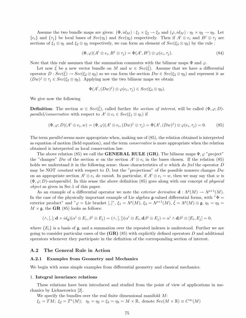
Assume the two bundle maps are given: (Φ, idM ) : ξ1 × ξ2 → ξ3 and (ϕ, idM ) : η1 × η2 → η3. Letei and τj be local bases of Sec(η1) and Sec(η2) respectively. Then if Ai ⊗ ei and Bj ⊗ τj aresections of ξ1 ⊗ η1 and ξ2 ⊗ η2 respectively, we can form an element of Sec(ξ3 ⊗ η3) by the rule :

(Φ, ϕ)(Ai ⊗ ei, Bj ⊗ τj) = Φ(Ai, Bj) ⊗ ϕ(ei, τj). (84)

Note that this rule assumes that the summation commutes with the bilinear maps Φ and ϕ.Let now ξ be a new vector bundle on M and w ∈ Sec(ξ). Assume that we have a differential

operator D : Sec(ξ) → Sec(ξ2 ⊗ η2) so we can form the section Dw ∈ Sec(ξ2 ⊗ η2) and represent it as(Dw)j ⊗ τj ∈ Sec(ξ2 ⊗ η2). Applying now the two bilinear maps we obtain

Φ(Ai, (Dw)j) ⊗ ϕ(ei, τj) ∈ Sec(ξ3 ⊗ η3).

We give now the following

Definition: The section w ∈ Sec(ξ), called further the section of interest, will be called (Φ, ϕ;D)-parallel/conservative with respect to Ai ⊗ ei ∈ Sec(ξ1 ⊗ η1) if

(Φ, ϕ;D)(Ai ⊗ ei, w) = (Φ, ϕ)(Ai ⊗ ei, (Dw)j ⊗ τj) = Φ(Ai, (Dw)j) ⊗ ϕ(ei, τj) = 0. (85)

The term parallel seems more appropriate when, making use of (85), the relation obtained is interpretedas equation of motion (field equation), and the term conservative is more appropriate when the relationobtained is interpreted as local conservation law.

The above relation (85) we call the GENERAL RULE (GR). The bilinear maps Φ, ϕ ”project”the ”changes” Dw of the section w on the section Ai ⊗ ei in the bases chosen. If the relation (85)holds we understand it in the following sense: those characteristics of w which do feel the operator Dmay be NOT constant with respect to D, but the ”projections” of the possible nonzero changes Dwon an appropriate section Ai ⊗ ei do vanish. In particular, if Ai ⊗ ei = w, then we may say that w is(Φ, ϕ;D)-autoparallel. In this sense the above definition (85) goes along with our concept of physicalobject as given in Sec.1 of this paper.

As an example of a differential operator we note the exterior derivative d : Λp(M) → Λp+1(M).In the case of the physically important example of Lie algebra g-valued differential forms, with ”Φ =exterior product” and ”ϕ = Lie bracket [, ]”, ξ1 = Λp(M), ξ2 = Λp+1(M), ξ = Λp(M) ⊗ g, η1 = η2 =M × g, the GR (85) looks as follows:

(∧, [, ];d × idg)(αi ⊗ Ei, β

j ⊗ Ej) = (∧, [, ])(αi ⊗ Ei,dβj ⊗ Ej) = αi ∧ dβj ⊗ [Ei, Ej ] = 0,

where Ei is a basis of g, and a summation over the repeated indexes is understood. Further we aregoing to consider particular cases of the (GR) (85) with explicitly defined operators D and additionaloperators whenever they participate in the definition of the corresponding section of interest.

A.2 The General Rule in Action

A.2.1 Examples from Geometry and Mechanics

We begin with some simple examples from differential geometry and classical mechanics.

1. Integral invariance relations

These relations have been introduced and studied from the point of view of applications in me-chanics by Lichnerowicz [2].

We specify the bundles over the real finite dimensional manifold M :ξ1 = TM ; ξ2 = T ∗(M); η1 = η2 = ξ3 = η3 = M × R, denote Sec(M × R) ≡ C∞(M)

75

Φ=substitution operator, denoted by i(X),X ∈ Sec(TM);ϕ=point-wise product of functions.We denote by 1 the function f(x) = 1, x ∈M . Consider the sections

X ⊗ 1 ∈ Sec(TM ⊗ (M × R)); α⊗ 1 ∈ Sec(T ∗M ⊗ (M × R)). Then the GR leads to

(Φ, ϕ)(X ⊗ 1, α ⊗ 1) = i(X)α ⊗ 1 = i(X)α = 0. (86)

We introduce now the differential operator d: if α is an exact 1-form, α = df , so that ξ = M × R,the GR gives

(Φ, ϕ;d)(X ⊗ 1, f) = (Φ, ϕ)(X ⊗ 1,df ⊗ 1) = i(X)df ⊗ (1 ⊗ 1) = i(X)df = X(f) = 0.

i.e. the derivative of f along the vector field X is equal to zero. So, we obtain the well known relation,defining the first integrals f of the dynamical system determined by the vector field X. In this sensef may be called (Φ, ϕ,d)-conservative with respect to X, where Φ and ϕ are defined above.

2.Absolute and relative integral invariants

These quantities have been introduced and studied in mechanics by Cartan [3]. By definition, ap-form α is called an absolute integral invariant of the vector field X if i(X)α = 0 and i(X)dα = 0.And α is called a relative integral invariant of the field X if i(X)dα = 0. So, in our terminology (thesame bundle picture as above), we can call the relative integral invariants of X (Φ, ϕ;d)-conservativewith respect to X, and the absolute integral invariants of X are additionally (Φ, ϕ)-conservative withrespect to X, with (Φ, ϕ) as defined above. A special case is when p = n, and ω ∈ Λn(M) is a volumeform on M .

3. Symplectic geometry and mechanics

Symplectic manifolds are even dimensional and have a distinguished nondegenerate closed 2-formω, dω = 0. This structure may be defined in terms of the GR in the following way. Choose ξ1 =η1 = η2 = M ×R, ξ2 ⊗ η2 = Λ3(T ∗M)⊗R, and d as a differential operator. Consider now the section1 ∈ Sec(M × R) and ω ∈ Sec(Λ2(T ∗M), with ω - nondegenerate. The map Φ is the product f.ω andthe map ϕ is the product of functions. So, we have

(Φ, ϕ;d)(1 ⊗ 1, ω) = Φ(1,dω) ⊗ ϕ(1, 1) = dω = 0.

Hence, the relation dω = 0 is equivalent to the requirement ω to be (Φ, ϕ;d)-parallel with respect tothe section 1 ⊗ 1.

The hamiltonian vector fields X are defined by the condition LXω = di(X)ω = 0. If Φ = ϕ is thepoint-wise product of functions we have

(Φ, ϕ;d)(1 ⊗ 1, i(X)ω) = (Φ, ϕ)(1 ⊗ 1,di(X)(ω) ⊗ 1) = LXω ⊗ 1 = LXω = 0.

In terms of the GR we can say that X is hamiltonian if i(X)ω is (Φ, ϕ;d)-parallel with respect to1 ⊗ 1.

The induced Poisson structure f, g, is given in terms of the GR by setting Φ = ω−1, whereω−1.ω = idTM , ϕ=point-wise product of functions, and 1 ∈ Sec(M × R). We get

(Φ, ϕ)(df ⊗ 1,dg ⊗ 1) = ω−1(df,dg) ⊗ 1.

A closed 1-form α, dα = 0, is a first integral of the hamiltonian system Z, di(Z)ω = 0, if i(Z)α =0. In terms of the GR we can say that the first integrals α are (i, ϕ)-parallel with respect to Z:(i, ϕ)(Z ⊗ 1, α ⊗ 1) = i(Z)α ⊗ 1 = 0. From LZω = 0 it follows LZω

−1 = 0. The Poisson bracket(α, β) of two first integrals α and β is equal to [−d(ω−1(α, β))] [6]. The well known property thatthe Poisson bracket of two first integrals of Z is again a first integral of Z may be formulated as: thefunction ω−1(α, β) is (i, ϕ;d)-parallel with respect to Z,

(i, ϕ;d)(Z ⊗ 1, ω−1(α, β)) = i(Z)dω−1(α, β) ⊗ 1 = 0.

76

A.2.2 Frobenius integrability theorems and linear connections

1.Frobenius integrability theorems [4]

Let ∆ = (X1, . . . ,Xr) be a differential system on M , i.e. the vector fields Xi, i = 1, . . . , r definea locally stable submodule of Sec(TM) and at every point p ∈ M the subspace ∆r

p ⊂ Tp(M) hasdimension r. Then ∆r is called involutive (or integrable) if [Xi,Xj ] ∈ ∆r, i, j = 1, . . . , r. Denote by∆n−r

p ⊂ Tp(M) a complimentary subspace: ∆rp ⊕ ∆n−r

p = Tp(M), and let π : Tp(M) → ∆n−rp be the

corresponding projection. So, the corresponding Frobenius integrability condition means π([Xi,Xj ]) =0, i, j = 1, . . . , r.

In terms of the GR we set D(Xi) = π LXi, Φ=”product of functions and vector fields”, and ϕ

again the product of functions. The integrability condition now is

(Φ, ϕ;D(Xi))(1 ⊗ 1,Xj)

= (Φ, ϕ)(1 ⊗ 1, π([Xi,Xj ] ⊗ 1)) = 1.π([Xi,Xj ]) ⊗ 1 = 0, i, j = 1, . . . , r.

In the dual formulation we have the Pfaff system ∆∗n−r, generated by the linearly independent

1-forms (α1, . . . , αn−r), such that αm(Xi) = 0, i = 1, . . . r;m = 1, . . . n− r. Then ∆∗n−r is integrable if

dα ∧ α1 ∧ · · · ∧ αn−r = 0, α ∈ ∆∗n−r. In terms of GR we set ϕ the same as above, Φ = ∧ and d as

differential operator and obtain

(Φ, ϕ;d)(α1 ∧ · · · ∧ αn−r ⊗ 1, α) = (∧, ϕ)(α1 ∧ · · · ∧ αn−r ⊗ 1,dα ⊗ 1)

= dα ∧ α1 ∧ · · · ∧ αn−r ⊗ ϕ(1, 1) = dα ∧ α1 ∧ · · · ∧ αn−r = 0,

i.e. α is (Φ, ϕ;d)-parallel with respect to α1 ∧ · · · ∧ αn−r ⊗ 1.

2. Linear connections

The concept of a linear connection in a vector bundle has proved to be of great importance ingeometry and physics. In fact, it allows to differentiate sections of vector bundles along vector fields,which is a basic operation in differential geometry, and in theoretical physics the physical fields arerepresented mainly by sections of vector bundles. We recall now how one comes to it.

Let f : Rn → R be a differentiable function. Then we can find its differential df . The map f → df

is R-linear: d(κ.f) = κ.df , κ ∈ R, and it has the derivative property d(f.g) = fdg+ gdf . These twoproperties are characteristic ones, and they are carried to the bundle situation as follows.

Let ξ be a vector bundle over M . We always have the trivial bundle ξo = M × R. Consider nowf ∈ C∞(M) as a section of ξo. We note that Sec(ξo) = C∞(M) is a module over itself, so we canform df with the above two characteristic properties. The new object df lives in the space Λ1(M)of 1-forms on M , so it defines a linear map df : Sec(TM) → Sec(ξo),df(X) = X(f). Hence, wehave a map ∇ from Sec(ξo) to the 1-forms with values in Sec(ξo), and this map has the above twocharacteristic properties. We say that ∇ defines a linear connection in the vector bundle ξo.

In the general case the sections Sec(ξ) of the vector bundle ξ form a module over C∞(M). So, alinear connection ∇ in ξ is a R-linear map ∇ : Sec(ξ) → Λ1(M, ξ). In other words, ∇ sends a sectionσ ∈ Sec(ξ) to a 1-form ∇σ valued in Sec(ξ) in such a way, that

∇(k σ) = k∇(σ), ∇(f σ) = df ⊗ σ + f ∇(σ), (87)

where k ∈ R and f ∈ C∞(M). If X ∈ Sec(TM) then we have the composition i(X) ∇, so that

i(X) ∇(f σ) = X(f)σ + f ∇X(σ),

where ∇X(σ) ∈ Sec(ξ).

77

In terms of the GR we put ξ1 = TM = ξ and ξ2 = Λ1(M) ⊗ ξ, and η1 = η2 = ξo. Also,Φ(X,∇σ) = ∇Xσ and ϕ(f, g) = f.g. Hence, we obtain

(Φ, ϕ;∇)(X ⊗ 1, σ) = (Φ, ϕ)(X ⊗ 1, (∇σ) ⊗ 1) = ∇Xσ ⊗ 1 = ∇Xσ, (88)

and the section σ is called ∇-parallel with respect to X if ∇Xσ = 0.

3. Covariant exterior derivative

The space of ξ-valued p-forms Λp(M, ξ) on M is isomorphic to Λp(M)⊗Sec(ξ). So, if (σ1, . . . , σr) isa local basis of Sec(ξ), every Ψ ∈ Λp(M, ξ) is represented by ψi ⊗ σi, i = 1, . . . , r, where ψi ∈ Λp(M).Clearly the space Λ(M, ξ) = Σn

p=0Λp(M, ξ), where Λo(M, ξ) = Sec(ξ), is a Λ(M) = Σn

p=0Λp(M)-

module: α.Ψ = α ∧ Ψ = (α ∧ ψi) ⊗ σi.A linear connection ∇ in ξ generates covariant exterior derivative D : Λp(M, ξ) → Λp+1(M, ξ) in

Λ(M, ξ) according to the rule

DΨ = D(ψi ⊗ σi) = dψi ⊗ σi + (−1)pψi ∧∇(σi)

= (dψi + (−1)pψj ∧ Γiµjdx

µ) ⊗ σi = (DΨ)i ⊗ σi.

We may call now a ξ-valued p-form Ψ ∇-parallel if DΨ = 0, and (X,∇)-parallel if i(X)DΨ = 0. Thisdefinition extends in a natural way to q-vectors with q ≤ p. Actually, the substitution operator i(X)extends to (decomposable) q-vectors X1 ∧X2 ∧ · · · ∧Xq as follows:

i(X1 ∧X2 ∧ · · · ∧Xq)Ψ = i(Xq) i(X)q−1 · · · i(X1)Ψ,

and extends to nondecomposable q-vectors by linearity. Hence, if Θ is a section of Λq(TM) we maycall Ψ (Θ,∇)-parallel if i(Θ)DΨ = 0.

Denote now by Lξ the vector bundle of (linear) homomorphisms (Π, id) : ξ → ξ, and let Π ∈Sec(Lξ). Let χ ∈ Sec(Λq(TM)⊗Lξ) be represented as Θ⊗Π. The map Φ will act as: Φ(Θ,Ψ) = i(Θ)Ψ,

and the map ϕ will act as: ϕ(Π, σi) = Π(σi). So, if ∇(σk) = Γjµkdx

µ ⊗ σj , we may call Ψ (∇)-parallelwith respect to χ = Θ ⊗ Π if

(Φ, ϕ;D)(Θ ⊗ Π,Ψ = ψi ⊗ σi) = (Φ, ϕ)(Θ ⊗ Π, (DΨ)i ⊗ σi) = i(Θ)(DΨ)i ⊗ Π(σi) = 0. (89)

If we have isomorphisms ⊗pTM ∽ ⊗pT ∗M,p = 1, 2, . . . , defined in some natural way (e.g. througha metric tensor field), then to any p-form α corresponds unique p-vector α. In this case we may talkabout ”∽”- autopaparallel objects with respect a (point-wise) bilinear map ϕ : (ξ × ξ) → η, where ηis also a vector bundle over M . So, Ψ = αk ⊗ σk ∈ Λp(M, ξ) may be called (i, ϕ;∇)-autoparallel withrespect to the isomorphism ”∽” if

(i, ϕ;∇)(αk ⊗ σk, αm ⊗ σm)

= i(αk)dαm ⊗ ϕ(σk, σm) + (−1)pi(αk)(αj ∧ Γmµjdx

µ) ⊗ ϕ(σk, σm)

=[i(αk)dαm + (−1)pi(αk)(αj ∧ Γm

µjdxµ)]⊗ ϕ(σk, σm) = 0.

(90)

Although the above examples do not, of course, give a complete list of the possible applications of theGR (85), they will serve as a good basis for the physical applications we are going to consider further.

A.3 Physical applications of GR

1. Autoparallel vector fields and 1-forms

In nonrelativistic and relativistic mechanics the vector fields X on a manifold M are the localrepresentatives (velocity vectors) of the evolution trajectories for point-like objects. The condition

78

that a particle is free is mathematically represented by the requirement that the corresponding vectorfield X is autoparallel with respect to a given connection ∇ (covariant derivative) in TM :

i(X)∇X = 0, or in components, Xσ∇σXµ + Γµ

σνXσXν = 0. (91)

In view of the physical interpretation of X as velocity vector field the usual latter used instead ofX is u. The above equation (91) presents a system of nonlinear partial differential equations for thecomponents Xµ, or uµ. When reduced to 1-dimensional submanifold which is parametrized locally bythe appropriately chosen parameter s, (91) gives a system of ordinary differential equations:

d2xµ

ds2+ Γµ

σν

dxν

ds

dxν

ds= 0, (92)

and (92) are known as ODE defining the geodesic (with respect to Γ) lines in M . When M isriemannian with metric tensor g and Γ the corresponding Levi-Civita connection, i.e. ∇g = 0 andΓµ

νσ = Γµσν , then the solutions of (92) give the extreme (shortest or longest) distance

∫ b

ads between

the two points a, b ∈M , so (92) are equivalent to

δ

(∫ b

a

ds

)= δ

(∫ b

a

√gµν

dxµ

ds

dxν

ds

)= 0.

A system of particles that move along the solutions to (92) with g-the Minkowski metric and gµνdxµ

dsdxν

ds>

0, is said to form an inertial frame of reference.It is interesting to note that the system (91) has (3+1)-soliton-like (even spatially finite) solutions

on Minkowski space-time [5]. In fact, in canonical coordinates (x1, x2, x3, x4) = (x, y, z, ξ = ct) letuµ = (0, 0,±v

cf, f) be the components of u, where 0 < v = const < c, and c is the velocity of light, so

vc< 1 and uσuσ =

(1 − v2

c2

)f2 > 0. Then every function f of the kind

f(x, y, z, ξ) = f(x, y, α(z ∓ v

cξ)), α = const, for example α =

1√1 − v2

c2

,

defines a solution to (91). If uσuσ = 0 then equations (91) (X = u), are equivalent to uµ(du)µν =

0, where d is the exterior derivative. In fact, since the connection used is riemannian, we have0 = ∇µ

12 (uνuν) = uν∇µuν , so the relation uν∇νuµ − uν∇µuν = 0 holds and is obviously equal to

uµ(du)µν = 0. The soliton-like solution is defined by u = (0, 0,±f, f) where the function f is of theform

f(x, y, z, ξ) = f(x, y, z ∓ ξ).

Clearly, for every autoparallel vector field u (or one-form u) there exists a canonical coordinate systemon the Minkowski space-time, in which u takes such a simple form: uµ = (0, 0, αf, f), α = const. Thedependence of f on the three spatial coordinates (x, y, z) is arbitrary , so it is allowed to be chosensoliton-like and, even, finite. Let now ρ be the mass-energy density function, so that ∇σ(ρuσ) = 0gives the mass-energy conservation, i.e. the function ρ defines those properties of our physical systemwhich identify the system during its evolution. In this way the tensor conservation law

∇σ(ρuσuµ) = (∇σρuσ)uµ + ρuσ∇σu

µ = 0

describes the two aspects of the physical system: its dynamics through equations (91) and its mass-energy conservation properties.

The properties described give a connection between free point-like objects and (3+1) soliton-likeautoparallel vector fields on Minkowski space-time. Moreover, they suggest that extended free ob-jects with more complicated space-time dynamical structure may be described by some appropriatelygeneralized concept of autoparallel mathematical objects.

79

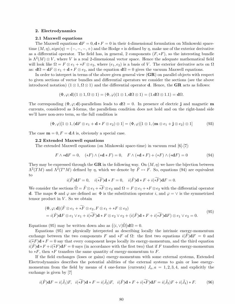
2. Electrodynamics

2.1 Maxwell equationsThe Maxwell equations dF = 0,d ∗F = 0 in their 4-dimensional formulation on Minkowski space-

time (M,η), sign(η) = (−,−,−,+) and the Hodge ∗ is defined by η, make use of the exterior derivativeas a differential operator. The field has, in general, 2 components (F, ∗F ), so the interesting bundleis Λ2(M) ⊗ V , where V is a real 2-dimensional vector space. Hence the adequate mathematical fieldwill look like Ω = F ⊗ e1 + ∗F ⊗ e2, where (e1, e2) is a basis of V . The exterior derivative acts on Ωas: dΩ = dF ⊗ e1 + d ∗ F ⊗ e2, and the equation dΩ = 0 gives the vacuum Maxwell equations.

In order to interpret in terms of the above given general view (GR) on parallel objects with respectto given sections of vector bundles and differential operators we consider the sections (see the aboveintroduced notation) (1 ⊗ 1,Ω ⊗ 1) and the differential operator d. Hence, the GR acts as follows:

(Φ, ϕ;d)(1 ⊗ 1,Ω ⊗ 1) = (Φ, ϕ)(1 ⊗ 1,dΩ ⊗ 1) = (1.dΩ ⊗ 1.1) = dΩ.

The corresponding (Φ, ϕ;d)-parallelism leads to dΩ = 0. In presence of electric j and magnetic mcurrents, considered as 3-forms, the parallelism condition does not hold and on the right-hand sidewe’ll have non-zero term, so the full condition is

(Φ, ϕ)[1 ⊗ 1, (dF ⊗ e1 + d ∗ F ⊗ e2) ⊗ 1] = (Φ, ϕ)[1 ⊗ 1, (m ⊗ e1 + j ⊗ e2) ⊗ 1] (93)

The case m = 0, F = dA is, obviously a special case.

2.2 Extended Maxwell equationsThe extended Maxwell equations (on Minkowski space-time) in vacuum read [6]-[7]:

F ∧ ∗dF = 0, (∗F ) ∧ (∗d ∗ F ) = 0, F ∧ (∗d ∗ F ) + (∗F ) ∧ (∗dF ) = 0 (94)

They may be expressed through the GR in the following way. On (M,η) we have the bijection betweenΛ2(TM) and Λ2(T ∗M) defined by η, which we denote by F ↔ F . So, equations (94) are equivalentto

i(F )dF = 0, i(∗F )d ∗ F = 0, i(F )d ∗ F + i(∗F )dF = 0.

We consider the sections Ω = F ⊗ e1 + ∗F ⊗ e2 and Ω = F ⊗ e1 +∗F ⊗ e2 with the differential operatord. The maps Φ and ϕ are defined as: Φ is the substitution operator i, and ϕ = ∨ is the symmetrizedtensor product in V . So we obtain

(Φ, ϕ;d)(F ⊗ e1 + ∗F ⊗ e2, F ⊗ e1 + ∗F ⊗ e2)

= i(F )dF ⊗ e1 ∨ e1 + i(∗F )d ∗ F ⊗ e2 ∨ e2 + (i(F )d ∗ F + i(∗F )dF ) ⊗ e1 ∨ e2 = 0.(95)

Equations (95) may be written down also as((i,∨)Ω

)dΩ = 0.

Equations (95) are physically interpreted as describing locally the intrinsic energy-momentumexchange between the two components F and ∗F of Ω: the first two equations i(F )dF = 0 andi(∗F )d ∗F = 0 say that every component keeps locally its energy-momentum, and the third equationi(F )d∗F + i(∗F )dF = 0 says (in accordance with the first two) that if F transfers energy-momentumto ∗F , then ∗F transfers the same quantity of energy-momentum to F .

If the field exchanges (loses or gains) energy-momentum with some external systems, ExtendedElectrodynamics describes the potential abilities of the external systems to gain or lose energy-momentum from the field by means of 4 one-forms (currents) Ja, a = 1, 2, 3, 4, and explicitly theexchange is given by [7]

i(F )dF = i(J1)F, i(∗F )d ∗ F = i(J2)F, i(F )d ∗ F + i(∗F )dF = i(J3)F + i(J4) ∗ F. (96)

80

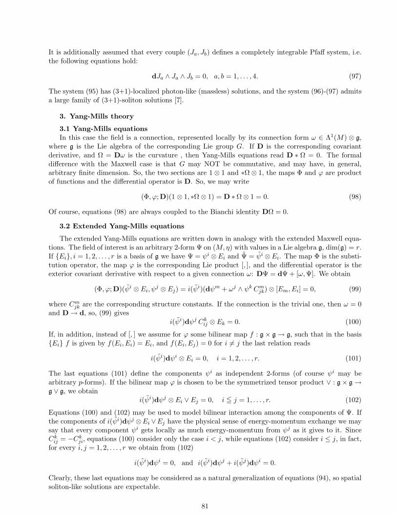
It is additionally assumed that every couple (Ja, Jb) defines a completely integrable Pfaff system, i.e.the following equations hold:

dJa ∧ Ja ∧ Jb = 0, a, b = 1, . . . , 4. (97)

The system (95) has (3+1)-localized photon-like (massless) solutions, and the system (96)-(97) admitsa large family of (3+1)-soliton solutions [7].

3. Yang-Mills theory

3.1 Yang-Mills equationsIn this case the field is a connection, represented locally by its connection form ω ∈ Λ1(M) ⊗ g,

where g is the Lie algebra of the corresponding Lie group G. If D is the corresponding covariantderivative, and Ω = Dω is the curvature , then Yang-Mills equations read D ∗ Ω = 0. The formaldifference with the Maxwell case is that G may NOT be commutative, and may have, in general,arbitrary finite dimension. So, the two sections are 1 ⊗ 1 and ∗Ω ⊗ 1, the maps Φ and ϕ are productof functions and the differential operator is D. So, we may write

(Φ, ϕ;D)(1 ⊗ 1, ∗Ω ⊗ 1) = D ∗ Ω ⊗ 1 = 0. (98)

Of course, equations (98) are always coupled to the Bianchi identity DΩ = 0.

3.2 Extended Yang-Mills equations

The extended Yang-Mills equations are written down in analogy with the extended Maxwell equa-tions. The field of interest is an arbitrary 2-form Ψ on (M,η) with values in a Lie algebra g, dim(g) = r.If Ei, i = 1, 2, . . . , r is a basis of g we have Ψ = ψi ⊗Ei and Ψ = ψi ⊗Ei. The map Φ is the substi-tution operator, the map ϕ is the corresponding Lie product [, ], and the differential operator is theexterior covariant derivative with respect to a given connection ω: DΨ = dΨ + [ω,Ψ]. We obtain

(Φ, ϕ;D)(ψi ⊗ Ei, ψj ⊗ Ej) = i(ψi)(dψm + ωj ∧ ψk Cm

jk) ⊗ [Em, Ei] = 0, (99)

where Cmjk are the corresponding structure constants. If the connection is the trivial one, then ω = 0

and D → d, so, (99) givesi(ψi)dψj Ck

ij ⊗ Ek = 0. (100)

If, in addition, instead of [, ] we assume for ϕ some bilinear map f : g × g → g, such that in the basisEi f is given by f(Ei, Ei) = Ei, and f(Ei, Ej) = 0 for i 6= j the last relation reads

i(ψi)dψi ⊗ Ei = 0, i = 1, 2, . . . , r. (101)

The last equations (101) define the components ψi as independent 2-forms (of course ψi may bearbitrary p-forms). If the bilinear map ϕ is chosen to be the symmetrized tensor product ∨ : g × g →g ∨ g, we obtain

i(ψi)dψj ⊗ Ei ∨ Ej = 0, i ≦ j = 1, . . . , r. (102)

Equations (100) and (102) may be used to model bilinear interaction among the components of Ψ. Ifthe components of i(ψi)dψj ⊗Ei ∨Ej have the physical sense of energy-momentum exchange we maysay that every component ψi gets locally as much energy-momentum from ψj as it gives to it. SinceCk

ij = −Ckji, equations (100) consider only the case i < j, while equations (102) consider i ≤ j, in fact,

for every i, j = 1, 2, . . . , r we obtain from (102)

i(ψi)dψi = 0, and i(ψi)dψj + i(ψj)dψi = 0.

Clearly, these last equations may be considered as a natural generalization of equations (94), so spatialsoliton-like solutions are expectable.

81

4. General Relativity

In General Relativity the field function of interest is in a definite sense identified with a Lorentzpseudometric g on a 4-dimensional manifold, and only those g are considered as appropriate to describethe real gravitational fields in vacuum which satisfy the equations Rµν = 0, where Rµν are thecomponents of the Ricci tensor. The main mathematical object which detects possible gravity is theRiemann curvature tensor Rαµ,βν , which is a second order nonlinear differential operator R : g → R(g).We define the map Φ to be the contraction, or taking a trace:

Φ : (gαβ , Rαµ,βν) = gαβRαµ,βν = Rµν ,

so it is obviously bilinear. The map ϕ is a product of functions, so the GR gives

(Φ, ϕ;R)(g ⊗ 1, g) = Φ[g ⊗ 1, R(g) ⊗ 1] = Φ[g,R(g)] ⊗ ϕ(1, 1) = Ric[R(g)] = 0. (103)

In presence of matter fields Ψa, a = 1, 2, . . . , r, the system of equations is

Rµν − κ

(Tµν − 1

2gµνT

)= 0.

It is easily obtained through the GR if we modify the differential operator Rαµ,βν to

Rαµ,βν − κ

2(Tαβgµν + Tµνgαβ − Tανgµβ − Tµβgαν) +

κ

3(gαβgµν − gανgµβ)T,

where κ is the gravitational constant, Tµν(Ψa) = Tνµ(Ψa) is the corresponding stress energy momen-tum tensor, and T = gµνTµν .

5. Schrodinger equation

The object of interest in this case is a map Ψ : R4 → C, and R

4 = R3 × R is parametrized by the

canonical coordinates (x, y, z; t), where t is the (absolute) time ”coordinate”. The operator D usedhere is

D = i~∂

∂t− H,

where H is the corresponding hamiltonian. The maps Φ and ϕ are products of functions, so the GRgives

(Φ, ϕ;D)(1 ⊗ 1,Ψ) =

(1 ⊗

(i~∂Ψ

∂t−HΨ

))⊗ 1 = 0. (104)

6. Dirac equation

The original free Dirac equation on the Minkowski space-time (M,η) makes use of the followingobjects: C

4 - the canonical 4-dimensional complex vector space, LC4-the space of C-linear mapsC

4 → C4, Ψ ∈ Sec(M × C

4), γ ∈ Sec(T ∗M ⊗ LC4), and the usual differential d : ψi ⊗ ei → dψi ⊗ ei,where ei, i = 1, 2, 3, 4, is a basis of C

4. We identify further LC4 with (C4)∗⊗C4 and if εi is a basis

of (C4)∗, dual to ei, we have the basis εi ⊗ ej of LC4 . Hence, we may write

γ = γjµidx

µ ⊗ (εi ⊗ ej),

and

γ(Ψ) = γjµidx

µ ⊗ (εi ⊗ ej)(ψk ⊗ ek)

= γjµidx

µ ⊗ ψk < εi, ek > ej = γjµidx

µ ⊗ ψkδikej = γj

µiψidxµ ⊗ ej.

82

The 4 matrices γµ satisfy γµγν+γνγµ = 2ηµνidC4 , so they are nondegenerate: det(γµ) 6= 0, µ = 1, 2, 3, 4,and we can find (γµ)−1 and introduce γ−1 by

γ−1 = ((γµ)−1)jidxµ ⊗ (εi ⊗ ej)

We introduce now the differential operators D± : Sec(M×C4) → Sec(T ∗M⊗C

4) through the formula:D± = id ± 1

2mγ−1, i =

√−1,m ∈ R. The corresponding maps are: Φ = η, ϕ : LC4 × C

4 → C4 given

by ϕ(α∗ ⊗ β, ρ) =< α∗, ρ > β. We obtain

(Φ, ϕ;D±)(γ,Ψ) = (Φ, ϕ)(γjµidx

µ ⊗ (εi ⊗ ej), i∂ψk

∂xνdxν ⊗ ek ± 1

2m(γ−1

ν )srdxν ⊗ (εr ⊗ es)ψ

mem)

= iγjµi

∂ψk

∂xνη(dxµ, dxν) < εi, ek > ej ±

1

2mγj

µi(γ−1ν )srψ

rη(dxµ, dxν) < εi, es > ej

= iηµνγjµi

∂ψk

∂xνδikej ±

1

2mηµνγj

µi(γ−1ν )srψ

rδisej

= iγµji

∂ψi

∂xµej ±

1

2m(−2δj

rψr)ej =

(iγµj

i

∂ψi

∂xµ∓mψj

)ej = 0

(105)

In terms of extended parallelism we can say that the Dirac equation is equivalent to the requirementthe section Ψ ∈ Sec(M × C

4) to be (η, ϕ;D±)-parallel with respect to the given γ ∈ Sec(M × LC4).Finally, in presence of external electromagnetic field A = Aµdx

µ the differential operators D± modifyto D± = (id − eA) ± 1

2mγ−1, where e is the electron charge.

A.4 Conclusion

It was shown that the GR, defined by relation (85), naturally generalizes the geometrical concept ofparallelism, and that it may be successfully used as a unified tool to represent formally importantequations in geometry and theoretical physics. If Ψ is the object of interest then the GR specifiesmainly the following things: the change DΨ of Ψ, the object Ψ1 with respect to which we consider thechange, the ”projection” of the change DΨ on Ψ1 through the bilinear map Φ, and the bilinear map ϕdetermines the space where the final object takes values. When Ψ = Ψ1 we may speak about autopar-allel objects in the corresponding sense, and in this case, as well as when the differential operator Ddepends on Ψ and its derivatives, we obtain nonlinear equation(s). In most of the examples consideredthe main differential operator used was the exterior derivative d and its covariant generalization.

In the case of vector fields and one-forms on the Minkowski space-time we recalled our previousresult that among the corresponding autoparallel vector fields there are finite (3+1) soliton-like ones,time-like, as well as isotropic. This is due to the fact that the trajectories of these fields define straightlines, so their ”transverse” components should be zero if the spatially finite (or localized) configurationmust move along these trajectories. Moreover, the corresponding equation can be easily modified tobe interpreted as local energy-momentum conservation relation.

It was further shown that Maxwell vacuum equations appear as d-parallel with somewhat trivialprojection procedure. This determines their linear nature and leads to the lack of spatial soliton-likesolutions. The vacuum extended Maxwell equations are naturally cast through the GR in the formof autoparallel (nonlinear) equations, and, as it was shown in our former works and in this review,they admit photon-like (3+1) spatially finite solutions, and some of them admit naturally defined spinproperties [8]. The general extended Maxwell equations (96) may also be given such a form if wereplace the operator d with (d− i(Ja)), and (3+1) soliton solutions of this system were also found [7].

The Yang-Mills equations were also described in this way. The corresponding extended Yang-Millsequations are expected to give spatial soliton solutions. The Einstein equations of General Relativityalso admit such a formulation.

83

In quantum physics the Schrodinger equation admits the ”parallel” formulation with trivial pro-jection. A bit more complicated was to put the Dirac equation in this formulation, and this is due tothe bit more complicated mathematical structure of γ = γj

µidxµ ⊗ (εi ⊗ ej).

These important examples make us think that the introduced here extended concept for (Φ, ϕ;D)-parallel/conservative objects as a natural generalization of the existing geometrical concept for ∇-parallel objects, may be successfully used in various directions, in particular, in searching for appro-priate nonlinearizations of the existing linear equations in theoretical and mathematical physics. Itmay also turn out to find it useful in looking for appropriate lagrangians in some cases. In our view,this is due to the fact that it expresses in a unified manner the dual change-conservation nature ofthe physical objects.

References to the Appendix

[1]. Greub, W. Multilinear Algebra, Springer, 1967[2]. Lichnerowicz, A., Les Relations Integrales d’Invariance et leurs Applications a la Dinamique,

Bull. Sc. Math., 70 (1946), 82-95[3]. Cartan, E., Lecons sur les Invariants integraux, Hermann & Fils, Paris, 1922[4]. Godbillon, C., Geometrie Differentielle et Mechanique Analytique, Hermann, Paris, 1969[5]. Donev, S., Autoclosed Differential Forms and (3+1)-Solitary Waves, Bulg. J. Phys., 15

(1988), 419-426[6]. Donev, S., Tashkova, M., Energy-momentum Directed Nonlinearization of Maxwell’s Pure

Field Equations, Proc. R. Soc. Lond. A, 443 (1993), 301-312[7]. Donev, S., Tashkova, M., Energy-momentum Directed Nonlinearization of Maxwell’s Equa-

tions in the Case of a Continuous Madia, Proc. R. Soc. Lond. A, 443 (1995), 281-291[8]. Donev, S., Screw Photon-like (3+1)-Solitons in Extended Electrodynamics, The European

Physical Journal ”B”, vol.29, No.2, 233-237 (2002).

84