Experimental Study of Multi-phase Flow Hydrodynamics In Stirring Tanks

Yihong Yang

Dissertation submitted to the faculty of the Virginia Polytechnic Institute and State University in partial fulfillment of the requirements for the degree of

Doctor of Philosophy

In Department of Engineering Science and Mechanics

Demetri P. Telionis (Committee Chair) Saad A. Ragab Ronald D. Kriz Roe-Hoan Yoon Gerald H. Luttrell

Feb 4, 2011 Blacksburg, VA

Keywords: multi-phase flow, turbulence, bubble-particle interaction, multi-hole probe,

isokinetic sampling probe, isokinetic borescope

©Copyright by Yihong Yang, 2011 All rights reserve

Experimental Study of Multi-phase Flow Hydrodynamics

In Stirring Tanks

Yihong Yang

ABSTRACT

Stirring tanks are very important equipments used for mixing, separating, chemical

reaction, etc. A typical stirring tank is a cylindrical vessel with an agitator driving the

fluid and generating turbulence to promote mixing. Flotation cells are widely used

stirring tanks in phase separation where multiphase flow is involved. Flotation refers to

the process in which air bubbles selectively pick up hydrophobic particles and separate

them from hydrophilic solids. This technology is used throughout the mining industry as

well as the chemical and petroleum industries.

In this research, efforts were made to investigate the multi-phase flow hydrodynamic

problems of some flotation cells at different geometrical scales. Pitot-static and five-hope

probes were employed to lab- pilot- and commercial-scale tanks for velocity

measurements. It was found that the tanks with different scales have similar flow patterns

over a range of Reynolds numbers. Based on the velocity measurement results, flotation

tanks’ performance was evaluated by checking the active volume in the bulk. A fast-

response five-hole probe was designed and fabricated to study the turbulence

characteristics in flotation cells under single- and multi-phase flow conditions. The jet

stream in the rotor-stator domain has much higher turbulence intensity compared with

other locations. The turbulent dissipation rate (TDR) in the rotor-stator domain is around

20 times higher than that near tank’s wall. The TDR could be used to calculate the bubble

and particle slip velocities. An isokinetic sampling probe system was developed to obtain

true samples in the multi-phase flow and then measure the local void fraction. It was

III

found that the air bubbles are carried out by the stream and dispersed to the whole bulk.

However, some of the bubbles accumulate in the inactive regions, where higher void

fractions were detected. The isokinetic sampling probe was then extended to be an

isokinetic borescope system, which was used to detect the bubble-particle aggregates in

the tank. Aggregates were found in the high-turbulence level zones. The isokinetic

sampling probe and the isokinetic borescope provide new methods for flotation tank tests.

An experiment was also set up to study the dynamics of bubble particle impact. Four

different modes were found for the collision. The criterion is that if the fluid drainage

time is less than the residence time, the attachment will occur, otherwise, the particle will

bounce back.

IV

Acknowledgements Upon the completion of the dissertation, I would like to take this opportunity to express

my appreciations to the people who have helped me and made the research work

possible.

First and foremost, I would like to thank my advisor and mentor, Dr. Demetri P. Telionis

for his guidance, inspiration and encouragement over the years. The communication

between us has three very interesting stages. We had very short conversation at the very

beginning due to the weakness of my oral English. He gave me a lot of useful suggestions

for my English practice. With great patience, Dr. Telionis even helped me to correct my

grammar and pronunciation word by word. Then the communications became smoother

and smoother, which leads to longer, deeper and hotter discussion, on both academic and

daily topics. After years’ learning and collaborating, my discussion with Dr. Telionsi

became briefer and briefer again because of the privity. No more redundant description

and explanation are needed since we can understand each other by saying even a word.

Even one word is not always necessary when I served as Captain Telionis’ crew to sail

the 22-foot long boat in Claytor Lake.

I appreciate the other members of my committee. Dr. Ronald D. Kriz is the first professor

that I talked and worked with after I came to USA. I still remember his advices on my

new life in our first conversation: communicate and be yourself. Working on the same

project, Dr. Saad A. Ragab, Dr. Roe-Hoan Yoon and Dr. Gerald H. Luttrell offered

numerous valuable discussions and suggestions as well as working conveniences. Thank

you for the time reviewing the dissertation and providing me with insightful comments.

Dr. Sunny Jung provided me with unreserved guidance in part of my research although

he is not in my committee. It is a great pleasure to work with him. I also want to thank

Dr. Pavlos Vlachos for his help and directions for the past years.

V

I am grateful to the other members of fluids lab at Virginia Tech especially Chris Denny

and Justin Watts. We are a great team and it has been a great pleasure to work together

closely over all these years. I also would like to recognize the contributions of my

colleagues: Hyusun Do, Abdel-Halim, Vasileios Vlachakis, Hassan Fayed, Sanja

Miskovic, Aaron Noble and Juan Ma.

The work leading to this dissertation was sponsored by FLSmidth Inc. Many thanks to

FLSmidth and its personnel: Asa Weber, Don Foreman and etc.

Thank my friends in Blacksburg and around the world.

Furthermore, I would like to thank my parents for their love and support. It is their

encouragement that keeps me going forward.

Finally, I would like to express my deepest gratitude to my wife, Dr. Qinqin Chen.

VI

Contributions

The following people have contributed to this dissertation scholarly. The brief description

of their contributions is listed as the followings.

Prof. Demetri P. Telionis: Committee chair and co-author. Provided guidance

throughout the entire research work, dissertation editing and proof reading.

Prof. Roe-Hoan Yoon: Committee member. Provided guidance in the research work in

Chapter 5.

Asst. Prof. Sunghwan(Sunny) Jung: professor, Department of Engineering Science and

Mechanics. Provided guidance in the research work in Chapter 5. Proposed the

theoretical analysis of bubble-particle interaction dynamics.

Aaron Noble: Ph.D. student, Department of Mining and Minerals Engineering. Provided

the test opportunities for bench test in bubble-particle aggregate detection experiments

described in Chapter 6.

VII

VIII

IX

List of Figures

 

 

X

XI

XII

XIII

List of Table

1  

Chapter 1 Introduction

1.1 Research background

Stirring tanks are very important pieces of equipment used for mixing, separating,

chemical reaction and other processes. A typical stirring tank is a cylindrical vessel

with an agitator driving the fluid and generating turbulence to enhance mixing. A

flotation cell is a stirring tank used for phase separation where multiphase flow is

involved. In the flotation process, air bubbles are used to pick up the valuable

minerals from waste gangue in hydrodynamic environment. The selected minerals are

either naturally hydrophobic, or hydrophobized by using reagents (collectors). When

the hydrophobic minerals collide with air bubbles, they attach to the bubbles and the

bubble/particle aggregates rise to the free surface, while the gangue particles stay in

the pulp. Controlling the minerals’ hydrophobicity and enhancing the bubble-particle

collision and attachment rates are of critical importance in flotation.

Flotation originated in Australia in the late 19th century. The first flotation plant in the

United States was constructed in 1911. In the early years, acid and oil were used as

the frothing agent. The first inventor making a clear claim for air as the flotation

media was Norris, as outlined in his 1907 patent[1].

Turbulence plays very important roles in flotation cells. The first role of turbulence in

flotation is enhancing solid suspension. Minerals have higher density than water, and

tend to sink down to the bottom. Turbulence keeps the particles suspended in the bulk.

To promote the mixing level, flotation cells are designed to achieve high turbulence

dissipation rate (ε) [2-5]. The second role of turbulence is bubble generation and air

dispersion. When air is pumped into the high-turbulence region, i.e. the rotor-stator

region, shearing forces break it into small bubbles and then the turbulent flow

disperses them into the entire vessel [6-8]. The third role of the turbulence is

2  

enhancing the bubble-particle collision rate by providing the particles and bubbles

with inertial energy [9-11]. Under turbulence conditions, bubbles and particle are well

mixed and move in random directions. When bubbles and particles approach each

other, a certain kinetic energy is needed to drain the fluid between them, and allow

them to collide. This energy is provided by turbulence

Flotation cells are normally run under multi-phase flow conditions. To simplify the

problems, single-phase flow were investigated first to study the hydrodynamic

characteristics, especially turbulence properties in the cells. Advanced

flow-measurement instruments, for example, Particle-Image Velocimetry (PIV), Laser

Dopper Velocimetry (LDV) and Planar Laser Induced Fluorescence(PLIF), have

been applied to measure the turbulence in different cells[12-14]. But these techniques

are mostly suited for laboratory work, and cannot be extended to two- and three-phase

flow.

Flotation is a very complicated process. It involves bubble and particle

hydrodynamics, bubble-bubble, particle-particle and bubble-particle interactions of

various characters, which is a challenge for theoretical description, experimental

detection and numerical simulation. Flotation machines are designed to maximize the

bubble-particle collision, however, since this process is highly stochastic, it is almost

impossible to measure the collision directly. Some models were developed to predict

the bubble-particle collision rate [9, 15, 16]. Those models can be simplified into a

general form.

(1.1)

where is the collision number, and and bubble and particle number

concentrations (PNC) and bubble and particle distance.

3  

Flotation kinetics is generally modeled as a first-principle rate process where

probability theory is adopted. The first-principle method assumes that attachments

and detachments occur simultaneously. For the attachment phenomenon, the rate is

assumed to be a function of the number concentrations of particles and bubbles, while

for detachment is related to the number concentrations of bubble-particle aggregate.

(1.2)

where k is the flotation constant, and P is another statistical parameter

characterizing the attachment and detachment probabilities. The attachment and

detachment rates depend on a wide range of complex factors, for example the

hydrodynamic characteristics of the tank and the sizes of bubble and particle. Yoon

studied the effect of bubble size on fine particle flotation[17].

In the present research project, efforts were made to investigate the hydrodynamic

problems of flotation cells at different scales. New instruments were designed and

constructed to characterize the multi-phase flow.

1.2 Statements of the problems

The performance of flotation cells is influenced by physical features and operating

conditions. Their efficiency depends critically on multi-phase flow hydrodynamics.

The bubble-particle collision can be enhanced by increasing the mixing level and

turbulence dissipation rate (TDR).On the other hand, excessive turbulence can also

break the bubble-particle aggregates and reduce the flotation efficiency. The aim is,

therefore, to create a proper level and extent of turbulence without enhancing the

detachment problem.

Over the years, many investigators studied the flow in flotation tanks. The studies

4  

conducted to date can be broadly classified into numerical simulations and

experimental measurements. To optimize the machine design, a better understanding

of the flows in flotation cells is necessary.

The trend towards large-capacity flotation machines has become more and more

obvious for the past decades. In the 1960’s, the size of a typical flotation tank was a

few cubic meters. In the 1970’s, the tanks’ capacity had been increased by an order of

magnitude. In the 2000’s, FLSmidth Minerals Inc. launched the 350m3 Super Cell,

which is the largest in the world. The benefits of large flotation machines include the

followings: (1) Reduced capital cost per ton of ore processed. (2) Reduced plant space

required. (3) Improved flotation section layout simplicity. (4) Reduced controls

complexity and improved flotation section operation. (5) Reduced maintenance costs.

(6) A possible reduction in power cost per ton of ore processed. Larger machine

design requires the development of reliable scale-up principles. Failure to establish a

basis for design scale-up will lead to high development costs, low machine efficiency

and loss in revenue. To reduce the application risk, machine scale-up design

procedure needs to be studied. Tests were conducted on lab- pilot- and

commercial-scale tanks for scale-up design procedure. New mechanisms were

designed based on this research and enhanced mineral recovery rate were achieved in

lab tests.

Hydrodynamics of large flotation cells involve very complex flow phenomena which

are hard to measure and model, for example, the bubble generation, the local void

fraction and turbulence energy dissipation. The study of such complex flows is of

great significance for the design of flotation cells. Progress in the experimental

investigation of the fluid mechanics of flotation cells is reported in this dissertation.

5  

1.3 Experimental models and facilities

The present studies were conducted on three Dorr-Oliver flotation cells, i.e. a 0.8 m3

lab cell, a 6 m3 pilot cell and a 160 m3 commercial cell. These three cells have special

stator and impeller geometries and are geometrically-similar (Fig.  1.1). Different

operation conditions and stator geometries are investigated. The wide range of the

sizes of these cells offers a unique opportunity to explore the effect of medium and

large Reynolds numbers, and the corresponding scaling laws.

 

 

Fig. 1.1 Dorr‐Oliver flotation tank: 6m3 pilot cell 

6  

 Fig. 1.2 Sketch of Dorr‐Oliver tank rotor‐stator assembly (side view) 

 

 Fig. 1.3 Sketch of Dorr‐Oliver tank rotor‐stator assembly (top view) 

The Dorr-Oliver cell consists of a cylindrical vessel with launder bevel, a 6-blade

impeller and a 16-blade stator (Fig. 1.2 and Fig. 1.3). The dimensions shown in Fig.

1.2 are normalized with the rotor diameter Di. For the lab cell, pilot cell and

commercial cell, the rotor diameters are 0.203m, 0.49 m and 2.442m respectively.

To test and calibrate instruments such as the isokinetic sampling probe and the

five-hole probe, a vertical bubbly flow tunnel was designed and built in the ESM

fluids laboratory (Fig. 1.4). This facility consists of a 50 gallon plastic container, a 1/4

horse power submersible pump, a 2” ID transparent pipe, a sparger system, tubing

system, some valves and some other accessories. Water is pumped into the sparger

chamber through 2” PVC pipes. A turbine liquid flow meter is installed between pipes

7  

to monitor the water flow rate. Air is injected into the sparger, which is a pipe rake

made of porous material, to generate bubbles. The bubbles mix with water in the

chamber. A honeycomb plate is installed in the inlet of the vertical test section to

generate uniform flow. The test section is 2” in diameter and 4’in length. After

passing through the test section, the flow returns to the container and the bubbles are

released at the water free surface in the quiescent environment. A surfactant, MIBC

(Methyl Isobutyl Carbinol), is mixed with water. The bubble size is controlled by

adjusting the MIBC concentration. The liquid flow meter and a gas flow meter are

used to measure the flow rate of the two phases respectively before they mix.

Readings of the flow meters can be used to calculate the average air fraction in the

test section. By adjusting the gas flow rate, we can get different air fractions.

 

 

Fig. 1.4 Vertical bubbly flow tunnel 

 

8  

  

Fig. 1.5 Multi‐phase high speed jet tunnel 

To test and calibrate some instruments such as isokinetic sampling probe and

five-hole probe, a high speed jet tunnel was designed and built (Fig. 1.5). This facility

is versatile since it can operate in single-phase flow as well as in multi-phase flow

conditions. It consists of a rectangular tank, tubing system, a centrifugal pump, a

T-shaped separating plate, a sponge, a sparger, a honeycomb structure, some valves

and some other accessories. The tank is 22”wide x 65” long x 20” deep. The

centrifugal pump is powered by a 3 horsepower electric motor, and its maximum

pumping capacity is 120 gallon/minute. The diameter of the jet tunnel nozzle can be

set as 2”, 1.5” and 1”. A honeycomb plate is installed ahead the nozzle to generate

uniform flow. The tubing system consists of 2” PVC pipes. A turbine flow meter

(Great Plains A1 Turbine Flow Meter) is set between pipes to monitor the flow rate.

The measuring range is 0.3 to 300 gallon/Minute. The T-shaped separating plate and

sparger are used only in two- and three-phase flow. For two-phase flow, air is injected

into the sparger to generate small bubbles. The surfactant (MIBC) is added to control

the bubble size. A gas flow meter is used to measure the gas flow rate. Combing the

liquid flow rate and the gas flow rate, we can calculate the air fraction of the jet flow.

When the flow returns from the nozzle side to the pump side, it will overflow the T

9  

plate where the bubbles rise and escape at the free surface. A sponge is put on the top

of the T plate to remove smaller bubbles. Hence what is sucked into the pump is

always single-phase fluid. This facility can also run in three-phase flow condition by

feeding particles into the pump inlet at a constant rate. As with the two-phase flow

operation, no particles can escape from nozzle side to the pump side. Since the motor

speed cannot be adjusted, the jet speed is controlled by adjusting the valves in the

piping system.

1.4 Research objectives

Flotation is a complicated process, the analysis of which involves colloid and surface

chemistry, hydrodynamics, thermodynamics, probability theory, and etc. Although

scientists have been working on it for about 150 years, some fundamental problems

are still far from being fully understood. For a specific industrial flotation cell, the

efficiency is controlled by many factors, such as blending level, particle suspension,

air dispersion and bubble-particle collision. This research work aims to develop new

test instruments and methods and use them to investigate the hydrodynamics of

multi-phase flow involved in flotation cells. The research topics include lab

environment experiments as well as the real machines tests. The objectives of this

research are to deepen the understanding of multi-phase flow in stirring tanks to

provide guidance on machine optimization and new machine design. Research on new

instrumentations and testing methodology are also discussed.

1.5 Organization of the dissertation

This dissertation is organized in terms of chapters that should stand alone as

independent documents. The plan is to be able to restructure them with minimal effort

in the form of papers that will later be submitted for publication in the open literature.

For this reason, each chapter has its own introduction and the review of relevant

10  

literature.

Chapter 2 consists of single-phase flow velocity measurements by using a five-hole

probe. In this chapter the flow fields of Dorr-Oliver cells were studied, which has

significant impact on the rotor-stator assembly design and feeding-exiting ports

arrangement. The flow field measurements also indicate the inactive zone, which

degrades the machines’ performance. Chapter 3 includes the development and

application of a novel instrument, the isokinetic sampling probe system. Using the

new instrument, local void fraction experiments were conducted to investigate the

tanks air dispersion capability. The influence of the flow pattern and multi-phase flow

characteristics were studied. In chapter 4, the development of a fast-response

five-hole water probe for turbulence measurements is described and the test results are

presented for different operation conditions. The turbulence characteristic, especially

the turbulent intensity and turbulence dissipation are discussed. In Chapter 5, a new

device and experiment is designed to study bubble-particle interaction dynamics.

Criteria of bubble-particle attachment and detachment were proposed based on the

measurements and theoretical analysis. Conclusions are included in individual

chapters. Chapter 6 contains a summary and a brief outlook for the future work.

11  

References 1. Parekh, B.K. and J.D. Miller, Advances In Flotation Technology. 1999:

Society for Mining, Metallurgy and Exploration, Inc.

2. Zughbi, H.D. and M.A. Rakib, Mixing in a fluid jet agitated tank: effects of jet

angles and elevation and number of jets. Chemical Engineering Science, 2004.

59: p. 829-842.

3. Yao, W.G., et al., Mixing performance experiments in impeller stirred tanks

subjected to unsteady rotational speed. Chemical Engineering Science, 1998.

53(17): p. 3031-3040.

4. Bittorf, K.J. and S.M. Kresta, Active volume of mean circulation for stirred

tanks agitated with axial impellers. Chemical Engineering Science, 2000. 55:

p. 1325-1335.

5. Alvarez-Hernandez, M.M., et al., Practical chaotic mixing. Chemical

Engineering Science, 2002. 57: p. 3749-3753.

6. Wang, T., J. Wang, and Y. Jin, A novel theoretical breakup kernel function for

bubble/dropletes in a turbulent flow. Chemical Engineering Science, 2003. 58:

p. 4629-4637.

7. Zhao, H. and W. Ge, A theoretical bubble breakup model for slurry beds or

three-phase fluidized beds under high pressure. Chemical Engineering Science,

2007. 62: p. 109-115.

8. Risso, F. and J. Fabre, Oscillations and breakup of a bubble immersed in

turbulent field. Journal of Fluid Mechanics, 1998. 372: p. 323-355.

9. Abrahamson, J., Collision rates of small particles in a vigorously turbulent

fluid. Chemical Engineering Science, 1975. 30: p. 9.

10. Koh, P.T.L., M. Manickan, and M.P. Schwarz, CFD simulation of

bubble-particle collisions in mineral flotation cells. Mineral Engineering,

2000. 13(14-15): p. 9.

11. Koh, P.T.L. and M.P. Schwarz, CFD Modeling of Bubble-Particle Collision

Rates and Efficiencies in a Flotation Cell. Minerals Engineering, 2003. 16: p.

12  

5.

12. Sharp, K.V. and R.J. Adrian, PIV study of small-scale flow structure around

Rushton turbine. AIChE Journal, 2001. 47(4): p. 766-778.

13. Law, A.W.K. and Wang. H., Measurement of Mixing Processes With Combined

Digital Particle Image Velocimetry and Planar Laser Induced Fluorescence.

Experimental Thermal and Fluid Science, 2000. 22: p. 213-229.

14. Schafer, M., M. Hofken, and F. Durst, Detailed LDV Measurements For

Visualization of The Flow Field Within A Stirred-Tank Reactor Equipped With

A Ruston Turbine. Trans IChemE, 1997. 75: p. 729-736.

15. Kruis, F.E. and K.A. Kusters, The collision rate of particles in turbulent flow.

Chemical Engineering Communications, 1997. 158: p. 201-230.

16. Pyke, B., D. Fornasiero, and J. Ralston, Bubble particle heterocoagulation

under turbulent conditions. Journal of Colloid and Interface Science, 2003.

265(1): p. 141-151.

17. Yoon, R.H. and G.H. Luttrell, The effect of bubble size on fine particle

flotation. Mineral Processing and Extractive Metallurgy Review, 1989. 5: p.

101-122.

13   

Chapter 2 Hydrodynamics of the Single-phase Flow

The flow in stirring tanks is very complicated because it passes around the rotating

impeller blades, interacts with stationary baffles or stator blades leading to

high-intensity turbulence, and develops flow loops and returns to the rotor region.

This chapter describes measurements and results obtained by traversing a five-hole

probe and Pitot-static probe in different-size stirring tanks with similar geometries.

The majority of the measurements were conducted in a 6-m3 flotation cell, but unique

to this investigation are the measurements conducted with Pitot tubes in a 160-m3

geometrically-similar full-scale tank. This provides the great opportunity to explore

how such flows scale with size and speed, extending to Reynolds numbers that

approach ten million.

2.1 Introduction

Stirring tanks are industrial devices which are extensively used to promote mixing,

separation, chemical reactions, and other industrial processes. A typical stirring tank is

a cylindrical vessel in which an agitator drives the fluid, thus generating turbulence.

The flotation cell is a typical stirring tank used in mineral industry, water treatment

plants, and other industrial facilities. Flotation is a selective process for separating

minerals from gangue by using surfactants, wetting agents and air bubbles. In the

mining industry, flotation efficiency depends critically on the initial collision between

air bubbles and mineral particles. To enhance this collision, flotation cells are

designed to achieve high turbulence dissipation rates (ε) and mixing level[1-5].

Flotation cells are generally designed as cylindrical tanks with rotor-stator assemblies.

Rotors can generate strong gradients in the flow by agitating the fluid, which leads to

high shear rates and high-intensity turbulence. The flow field generated by flat-bladed

14   

turbines in a cylindrical tank is divided into two distinct toroidal regions, one located

above and the other below the impeller top. As the aerated slurry exits between stator

blades, the flow changes rapidly, generating strongly anisotropic and inhomogeneous

patterns[6-11]. The study of such complex flows is of great significance for the design

of flotation cells. Better understanding of the flow features in these cells will lead to

improved design and performance, and reduction in maintenance costs.

The flow phenomena in flotation cells are very hard to simulate, model and measure.

Due to the great complexity of the flow, only some empirical relations rather than

theoretical analysis have been derived and used in flotation cell design. In some of

these relations, an average turbulent dissipation is widely used to characterize a cell,

while in others a Gaussian turbulent velocity distribution is used[1-4],. These

approaches can provide useful engineering guidelines, but are limited in accuracy and

cannot give information on spatial distributions of energy and fluid velocities.

Computational Fluid Dynamics (CFD) has emerged as a new tool to design more

efficient flotation machines, but its application has been limited to low Reynolds

numbers, and is difficult to use to predict three-phase flows. The relative motion

between the stationary parts and the rotating impeller is a considerable challenge.

Recent advances in CFD and other sophisticated analytical methods have generated

useful information at high Reynolds numbers, but experimental testing continues to

play a vital role in the development of high performance flotation cells. Designers

must resort to gathering performance data from production equipment operating in

non-laboratory environments.

A variety of experimental methods like hot-wire anemometry, Laser-Doppler

Velocimetry (LDV) and Particle Image Velocimetry (PIV) have been employed in the

past to measure the flow in small stirring tanks. Some efforts have been made to use

PIV in small laboratory flotation cell models[8-11]. But the most serious limitation of

15   

such methods is the need for optical access, which limits them to clear fluids and

transparent vessels. So far our understanding of these complicated processes is far

from complete and the limitations of experimental methods for their investigation are

very confining.

In this chapter, we describe efforts to investigate the single-phase flow hydrodynamics

in flotation processes. A five-hole probe was designed and fabricated for the velocity

measurements. The measurements were carried out in three geometrically similar

flotation cells. This gives us the opportunity to investigate the effect of scaling. The

majority of the flow measurements were conducted in a 6 m3 Dorr-Oliver pilot cell.

Our main objective is to measure the flow characteristics and then provide designers

with guiding information for product optimizations. Another objective is to study the

Reynolds number effects on machine performance by comparing the pilot cell data

with our results obtained in a smaller lab cell and a 160 m3 full-scale commercial cell.

These cells are geometrically-similar and their Reynolds numbers range from 104 to

106. To the knowledge of the author, experimental results of flotation obtained at

Reynolds numbers over 106 have not yet been presented in the literature.

2.2 Experiment methods and instruments The five-hole probe is a cost-effective, robust and accurate method for

three-dimensional velocity vector determination, which makes it practical for both

laboratory and field applications. Some advanced techniques such as Laser Doppler

Velocimetry (LDV) and Particle Image Velocimetry (PIV) have better accuracy

compared to five-hole probes, but the requirement of optical access to the domain of

interest limits their applications.

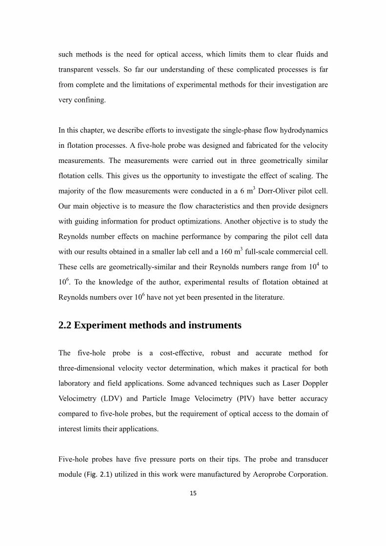
Five-hole probes have five pressure ports on their tips. The probe and transducer

module (Fig. 2.1) utilized in this work were manufactured by Aeroprobe Corporation.

16   

For the probes described here, the pressure ports are distributed on a conical tip. One

hole (port number 1) is located at the apex of the cone and the other holes (ports 2

through 5) are uniformly distributed around the central port, halfway downstream of

the apex (Fig.  2.2). This arrangement provides the capability of making accurate

measurements of flow angles of up to ±60o. The five-hole probe is calibrated by

inserting it in a flow field of known uniform velocity in magnitude and direction. It is

then rotated and pitched through a range of known angles to simulate all possible

measurable velocity inclination. For each of the specific angles, the pressures from all

the pressures ports are recorded and stored in a database. A calibrated probe can be

inserted into an unknown flow field to measure the velocity vector, by recording the

port pressures and comparing them with the calibration database through a set of

non-dimensional coefficients and interpolation equations. The velocity vector is

expressed in the local coordinate system and the flow incidence angles are denoted

using the following symbols: pitch (α) and yaw (β), or cone (θ) and roll (φ).

 Fig. 2.1 Fiver‐hole probe and transducer module 

 

 

  

 

2.2 The

bod

the

anal 

Wh

surf

ofte

max

pres

po=

The

the

flow

dist

.1 The wo

e principle o

dy is immers

direction an

lytically, bu

en a body

face varies

en lower th

ximum pres

ssure, p∞ an

=p∞+ρV∞2/2

e lowest pre

body is nea

w over blu

ribution and

Fig. 2.2 

orking pr

of multi-ho

sed in a stre

nd magnitud

ut in practice

is inserted

from a max

han the sta

ssure is equ

nd the dynam

2

ssures are f

arly paralle

ff bodies o

d introduces

Layout of t

rinciple of

ole probe m

eam, the pre

de of the str

e, probes ar

in the flow

ximum at t

atic pressur

ual to the t

mic pressure

found near t

el to the fre

often separ

s adverse pr17 

he pressure

f multi-ho

measurement

essure at spe

ream veloci

re calibrated

w of any flu

the stagnatio

re of the f

total pressur

e far from th

the regions w

e stream. T

ates. Flow

ressure grad

e ports on p

ole probe

ts is based

ecific points

ity. This rela

d experimen

uid, the pre

on point to

far upstrea

re, po whic

he body.

where the in

This of cour

separation

dients.

 

probe tip 

(MHP)

on the fact

s on its surf

ationship ca

ntally.

essure distri

o some low

am. For blu

ch is the su

nclination o

rse is not al

n alters the

t that if a b

face is relate

an be develo

ibution ove

values that

uff bodies,

um of the s

(2.

of the surfac

lways true.

local pres

bluff

ed to

oped

er its

t are

the

static

.1)

ce of

The

ssure

18   

In this dissertation, “far upstream”, “free stream”, and “conditions at infinity”,

denoted by the subscript ∞ imply a position upstream of the probe tip, where we

assume that the flow is uniform and unaffected by the presence of the probe. These

assumptions will need qualification. But in practice, this distance is on the order of the

probe tip diameter.

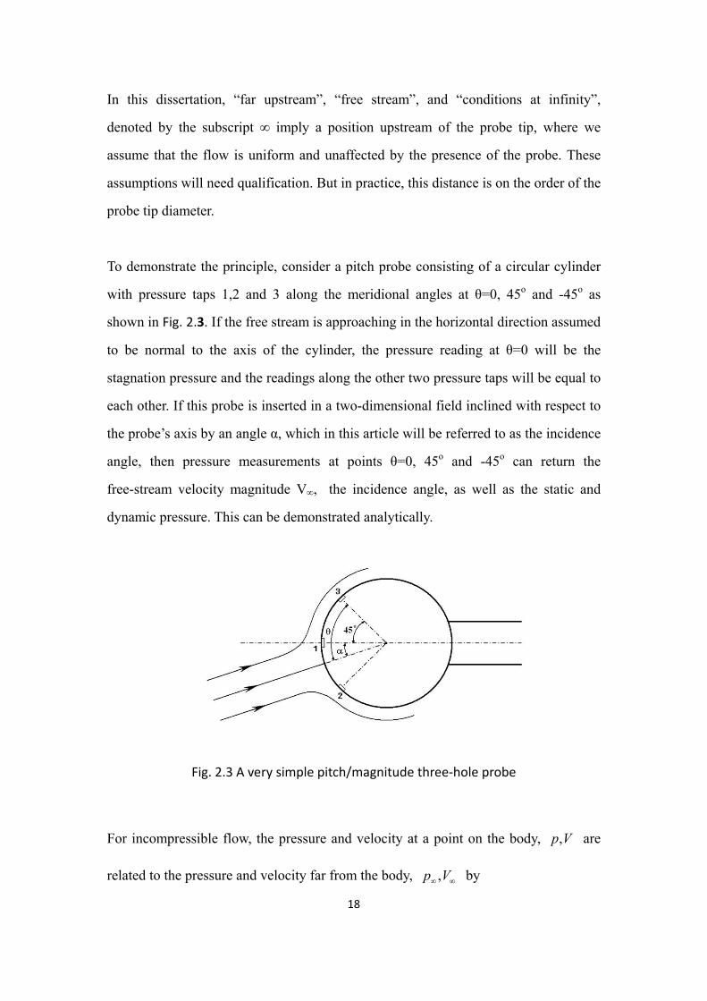
To demonstrate the principle, consider a pitch probe consisting of a circular cylinder

with pressure taps 1,2 and 3 along the meridional angles at θ=0, 45o and -45o as

shown in Fig. 2.3. If the free stream is approaching in the horizontal direction assumed

to be normal to the axis of the cylinder, the pressure reading at θ=0 will be the

stagnation pressure and the readings along the other two pressure taps will be equal to

each other. If this probe is inserted in a two-dimensional field inclined with respect to

the probe’s axis by an angle α, which in this article will be referred to as the incidence

angle, then pressure measurements at points θ=0, 45o and -45o can return the

free-stream velocity magnitude V∞, the incidence angle, as well as the static and

dynamic pressure. This can be demonstrated analytically.

 

 

Fig. 2.3 A very simple pitch/magnitude three‐hole probe 

For incompressible flow, the pressure and velocity at a point on the body, ,p V are

related to the pressure and velocity far from the body, ,p V∞ ∞ by

19   

p V p V (2.2)

For a circular cylinder, the potential flow solution gives the velocity on the cylinder as

V θ 2V sin θ (2.3)

where θ is the angular distance from the point of stagnation to the point of

interest.

We can then employ Eqs. (2.2) and (2.3) for the pressure at the three pressure taps as

follows:

P V =P(45° α)+ 2ρV sin 45° α (2.4)

P V =P(α)+ 2ρV sin α (2.5)

P V =P(45° α)+ 2ρV sin 45° α (2.6)

If the pressure at ports 1, 2 and 3 are measured, then the system of Eq.2.4 to Eq.2.6

can be solved for the unknowns ,p V∞ ∞ and α, which are the local value of the static

pressure, the local magnitude of the velocity and the slope of this velocity vector.

The basic idea is now to design a probe with a tip shape that will involve measurable

variations of the pressure that can be associated with the direction and magnitude of

the local velocity vector. Pressure taps are placed along the tip of the probe at

locations that will involve measureable variations of the local pressure, associated

with the magnitude and direction of the flow.

Analytical or numerical relations similar to those represented by Eq.2.4 to Eq.2.6

connecting pressure values on the probe tip to the local velocity, static and dynamic

pressure can be derived for any probe tip shape. But minor errors in the machining of

20   

the probe tip and the location of the pressure taps introduce measurement errors that

can only be eliminated by calibration. Probe calibration requires inserting the probe in

a known uniform flow field, traversing it along pitch and yaw angles and measuring

the corresponding pressures. Calibration processes are discussed later in this paper.

2.2.2 Calibration procedures

As with any instrument, calibration of MHP requires that the probe is exposed to a

series of combinations of parameter values it will be required to readThe data are

stored, and the mathematical operation is prepared for the use of the instrument as a

measuring device. The physical quantities that the user expects to obtain are the

magnitude and the direction of the flow velocity, the static and the dynamic pressure

at the point of measurement. All these quantities are functions of the pressures

measured by the pressure taps arranged on the tip of the probe. A typical numbering of

the tip pressure taps for a five-hole probe is shown in Fig. 2.2. The orientation of a

probe with respect to the oncoming free stream is defined in terms of two angles.

These could be cone and roll, θ and φ, or pitch and yaw, α β. The systems (θ,φ) and

(α,β) are completely interchangeable, and the conversion between them is given by

the following geometrical relations:

α tan tanθsin (2.7)

β sin sinθcos (2.8)

The calibration data are actually discrete data. When the instrument is used as a

measurement tool, the measured quantities fall between the discrete calibration data.

Software is applied for the efficient interpolation that can return measurements in

terms of the calibration files.

As explained in the following sections, the basic calibration parameters are the angles

21   

that define the orientation of the probe, the Reynolds number and the Mach number.

The dependence of the quantities to be measured on the calibration parameters is

described in terms of calibration surfaces. These surfaces are unique to each

instrument. Even if two probes are machined on computer-controlled equipment with

identical specifications and drawings, their calibration surfaces deviate from each

other. In other words, no two probes are identical to each other. This is because the

slightest mechanical discrepancies on the surface of the probe tips can induce

non-negligible differences in the calibration surfaces. This is why each probe must be

calibrated through the entire domain of the parameter values that it is expected to

encounter.

2.2.3 Calibration mechanisms

A calibration machine should be able to generate independently the discrete values of

two spatial attitude angles, the Reynolds number, Re and the Mach number, M:

Re=ρV∞L/μ (2.9)

Μ=V∞/a (2.10)

This means that the total temperature and total pressure of the free stream must be

known. Such machines must generate free streams with the lowest levels of

turbulence possible, and mechanisms that can position the probe at different spatial

orientations.

Free streams with varying Reynolds and Mach numbers can be generated by

closed-circuit wind tunnels or blow-down wind tunnels. In most facilities, it is not

possible to control independently the Mach number and the Reynolds number. This is

because if the density and temperature cannot be controlled independently, then

22   

increasing the speed of the tunnel results in increases of both the Reynolds number

and the Mach number. To control these parameters independently requires a facility

that can be operated at controlled pressures and/or temperatures. Such facilities are

too expensive to construct and operate. For most practical applications, the

dependence of the calibration surfaces on the Reynolds number is rather weak. It is

therefore adequate to calibrate for different values of the Mach number, and in

practice, this is achieved by increasing the speed of the tunnel.

A probe must be placed in the tunnel with its tip as close as possible to the middle of

the test section and be given angular displacements such that its tip is not linearly

displaced. In other words, the probe tip must remain at the same point in space while

its axis is given the required inclinations. This is necessary because even in the most

carefully designed tunnels there is some variation of the local velocity vector across

the test section.

The most common calibration mechanism that allows adjusting inclination angles

keeping the probe tip fixed in space is a U-shaped bracket that can rotate about an axis

that passes through its two tips as shown in Fig. 2.4. One of the U bracket legs is

mounted on a stepper motor that controls the cone angle. The other leg is essentially

the probe itself, or an extension of it, and this could be mounted at its base on a

stepper motor that controls its roll. The base includes a stepper motor to control

rolling, indicated by the curly arrow B. The disk G is mounted flash with the wall of

the test section, or is placed far from the calibration jet. The roll stepper motor E is

placed far from the roll axis, and rolling is achieved by a belt drive.

23   

Fig. 2.4 Calibration mechanism with motors to control cone and roll 

2.2.4 MHP use and applications Laboratory use In the first few decades of laboratory work in aerodynamics, the Pitot-static probe was

the only tool available to measure flow velocity. Multi-hole probes followed soon.

Then more sophisticated methods like hot-wire anemometry, laser-Doppler

velocimetry and more recently particle-image velocimeter provided more options to

the researchers. But the development of miniature pressure transducers, powerful

computers and sophisticated software led to the re-emergence of multi-hole probes.

Today MHPs compete with all other flow measurement tools, and their ease of use

and low price make them attractive to researchers and practicing engineers.

MHPs are used extensively in wind tunnels where they are first employed to calibrate

the tunnels by recording the uniformity of the flow in the test section. Such probes can

then be employed to map out the velocity field around aerodynamic models. They are

often used to generate data along a grid in the wake of an aircraft model, which can

then be used to estimate drag and lift, as well as the strength of the wing-tip vortices.

The same probes are often used to document the flow field around the model.

24   

MHPs are also employed in turbomachinery applications. They can generate the flow

properties downstream of the fan of a gas-turbine engine, between compressor stages,

and even in the exhaust region. The special MHPs like fast-response probes and

high-temperature probes are used widely in this area.

Field measurements Multi-hole probes are often employed for field measurements. They are used by many

different industries in monitoring smoke stack flows. They find applications in wind

engineering, monitoring wind speed and direction. But the most important practical

application is their use in detecting the pitch and yaw of aircraft. The MHP used in

this application is called the “air-data probe”. The tip of such a probe is essentially a

conventional five-hole probe tip. But about ten diameters from the tip, air-data probes

are usually equipped with a static ring, which consists of six to eight pressure ports

that record the local static pressure by pneumatically averaging their readings.

As for the commercial flotation cell measurement, a Pitot-Static rake, which consists

of 8 probes, is utilized. The rake was manually operated to move along a vertical shaft

collecting data at different locations.

2.2.5 Probe interference Any probe inserted in the flow will interfere with the flow, and the readings of any

probe will be influenced by the presence of bodies that are inserted in the flow. In

most cases, such interference is negligible, but on occasions it may be considerable. In

general, when the probe is placed in high receptivity areas, its effect on the flow may

be from non-negligible to dramatic.

25   

High receptivity regions of a flow are the regions where bifurcations can easily occur

through the introduction of a relatively small disturbance. In other words, these are

areas where a small energy/disturbance input causes dramatic changes to the flow

behavior. For example, the introduction of a small disturbance near the separation

point has the potential of swinging the flow from fully separated to fully attach and

vice versa. Placement of the probe in such regions is likely to affect the flow behavior.

The size of the probe and the hardware holding it in place is also an important factor.

By adequately miniaturizing the probe and the associated probe holder/positioning

hardware, it is possible to avoid such occurrences.

Probe in the upstream of body

If the probe is placed with its tip upstream of the body, there will be no interference

on the readings of the probe. Within its own accuracy, the probe will read the flow

features at the point it is placed, which are influenced by the body. The probe itself

may introduce very small disturbances to the flow over the body. These will depend

on the configuration under consideration. But if a probe is inserted close to the

stagnation streamline it is possible that disturbances may be introduced into the

boundary layer, and then induce transition to turbulence. This situation does not arise

in the measurements described in this dissertation.

Probe is away from the body

A probe placed in tandem with the body but five probe diameters away from its

surface will not introduce any interference, nor will its readings be affected by the

body. But if a probe is placed within the boundary layer, it may trip the boundary

layer, induce transition to turbulence, and affect the location of separation

significantly. In the present work, probes were placed either upstream or downstream

26   

of plates, and never close to their walls.

Probe in the wake

A probe placed in the free-shear layer may trip it to turbulence and influence the rate

at which this layer rolls to form large vortical structures. But in most practical cases

for Reynolds numbers larger than one hundred thousands, as is the case here, shear

layers are always turbulent. A probe placed in the wake will have no effect on the flow.

But it will not be able to provide good measurements, since the flow in this region

may be reversed. In the present experiments we turn the probe around in regions

where we expect the flow to be reversed. But there are still regions of intermittent

flow direction, and in such domains the measurements are discarded.

Probe in three-dimensional flows

The above statements are valid for flow over three-dimensional bodies. A special 3-D

case is axial vortices, like wing-tip, or delta-wing vortices. Such swirling vortices may

contain large longitudinal and circumferential velocity components. A probe inserted

close to the core of an axial vortex with its axis in line with the vortex axis may

induce vortex breakdown, and alter the flow drastically. Another problem arises if the

probe is inserted in an axial vortex with its axis in the circumferential direction. In

that case, strong gradients of the circumferential velocity component give rise to

radial pressure gradients, which are interpreted by the calibration software as large

radial velocity components. These are often called phantom,

2.3 Layout of the experiments

The five-hole probe system shown in Fig. 2.1 was used for flow field measurements

27   

in three Dorr Oliver flotation cells with the same geometry but different sizes, but

extensive measurements covering all the sectors of the machine were only obtained in

the 6 m3 Dorr-Oliver pilot cell (Fig. 2.5). The probe is mounted on a two-axes

traversing system which is controlled by a computer. The probe can also be translated

along the third axis manually (Fig. 2. 6). Small tubing is used to connect the probe to a

transducer module. To maximize the measurement accuracy, the tubing is kept as

short as possible. This is because the tubes are somewhat flexible, and may expand in

response to pressure variations. Fig. 2.7 and Fig. 2.8 show the sketch of the rotor-stator

assembly, as well as the coordinate system that we used. The Dorr-Oliver rotor has 6

blades while the stator has 16 blades. The origin of the coordinate system was set in

the middle of the rotor bottom. All the dimensions are normalized by rotor diameter,

Di.

 Fig. 2.5 6 m3 Dorr‐Oliver Pilot Cell 

 

28   

 Fig. 2. 6 Layout of the test 

 

 Fig. 2.7 Sketch of rotor‐stator assembly (side view) 

 

29   

 

Fig. 2.8 Sketch of rotor‐stator assembly (top view) 

 

 

 Fig. 2. 9 Coordinate transformation 

The five-hole probe returns results in the Cartesian coordinate system, i.e. Ux, Uy and

Uz. Since the flotation tanks are cylindrical, we transfer the velocity components to a

cylindrical coordinate system for description convenience. As shown in Fig. 2. 9, the

probe is aligned with the x-axis facing the rotor. It is therefore inclined by an angle θ

with respect to the radial direction.

(2.9)

30   

The velocity components can be written in cylindrical coordinates as follows:

sin (2.10)

(2.11)

(2.12)

Where, is the radial velocity, is the tangential velocity and is the

longitudinal velocity.

2.4 Results and discussions The flow pattern is of great significance to the designer. This information will be used

to optimize the geometries and layout of rotor, stator and vessel. It is also helpful to

arrange the slurry feeding and tailing ports. Figure 2.10 is the CFD result obtained by

the author using the commercial CFD software Fluent, which is presented here only to

qualitatively show the flow characteristics on the central vertical plane of the lab-scale

cell. It can be seen that the flow field is divided into two toroidal regions with

opposite sense of rotation. A strong jet emanates from the impeller, which can be

clearly distinguished in this plot. All our experimental results confirm that the flow is

dominated by a strong jet of a narrow cross-section.

31   

 Fig. 2.10 CFD result of Dorr‐Oliver flotation cell

 

Fig. 2.11 Velocity profiles along a vertical line in the Rotor‐Stator Gap: θ=11.25o, x/Di=0.571, normalized by Utip 

32   

The flow in the rotor-stator gap

The probe was placed firstly in the middle of the rotor-stator gap, which is

downstream of the rotor but upstream of the stator plates, where the influence of the

stator is not felt yet. Fig.  2.11 shows the three components of the velocity along a

vertical line. The results indicate that the rotor generates a jet stream on the upper

region. Not counting the thickness of the top rotor cover, the effective rotor height is

0.57Di. This means that the jet rushes out only in the 1/3 portion of the rotor. Besides

the radial component, the jet has very strong circumferential and longitudinal

velocities. The longitudinal and tangential velocities are even higher than the radial.

Since the jet has an upward component, does it escape for the rotor-stator gap?

Calculations based on our experimental data indicate that the jet is inclined upward by

an angle of =27o. Geometrical estimates indicated that escaping the gap would

require an angle of =31.5o as shown in Fig. 2.12. This means that the jet will hit

the lower surface of the stator’s annular ring and will not rush out upwards from the

gap between the rotor and stator. This result matches with the flow pattern shown in

Fig. 10.

 

  

Fig. 2.12 Elevation angle of the jet

 

33   

Fig. 2.11 also shows that negative radial velocities indicate that fluid is sucked into the

rotor in the lower region. Comparing with the jet stream, the returning flow is very

uniform and slow. Besides the radial velocity, the returning flow also has strong

circumferential and longitudinal components. The returning flow is also present in the

region where y/Di <0. Since y/Di=0 is the level of the rotor bottom, it indicates that

the fluids are also sucked into the clearance between rotor and the floor and then turns

upwards.

In the region where 0.2 < y/Di < 0.4, the flow does not have stable direction and

magnitude. This implies that there is a region of oscillating radial direction, where the

flow direction alternates pointing inward and outward. This region of intermittent

flow direction is in the middle of the rotor and covers 1/3 of the total rotor height.

The flow outside the stator

As described above, the fluid is driven out from the rotor region by the blades at a

certain angle, both circumferential and longitudinal. It then impinges on the stator

annular ring and the stator blades and moves radially outwards. It is expected that the

stator will change the flow pattern dramatically. To examine this assumption, and

explore the function of the stator, the five-hole probe was placed outside the stator to

measure the velocity. The traversing system was used to take data at specific points

along a vertical line.

34   

 Fig. 2.13 Radial velocity along horizontal lines x/Di= 1 (1” away from stator), 

y/Di=0.622, 0.571, 0.520 

As shown in Fig.  2.8, the stator has 16 blades, spaced uniformly under the annular

cover of the stator. Due to symmetry, the tank can be divided into 16 sectors in the

circumferential direction, and each sector must have the same flow pattern under

ideal conditions. Therefore the experiments were performed in one of the sectors as

shown in Fig. 2. 9 , namely, in the domain of 11.25o < < -11.25o. The stator blade

corresponds to =0.

In Fig. 2.13, we show the radial velocities along three horizontal lines at different

elevation (y/Di=0.622, 0.571, 0.520). We see that a jet stream shoots out form one side

(windward side) of the stator blade while on the other side (leeward side), the flow is

very quiet. So the zone outside the stator is split into two regions: active region (jet

region) and inactive region (wake region) and the circumferential ratio is almost 50:50

on the horizontal plane. By comparing the radial velocity magnitudes at different

elevation, we can see that the jet is stronger on the upper location.

35   

 

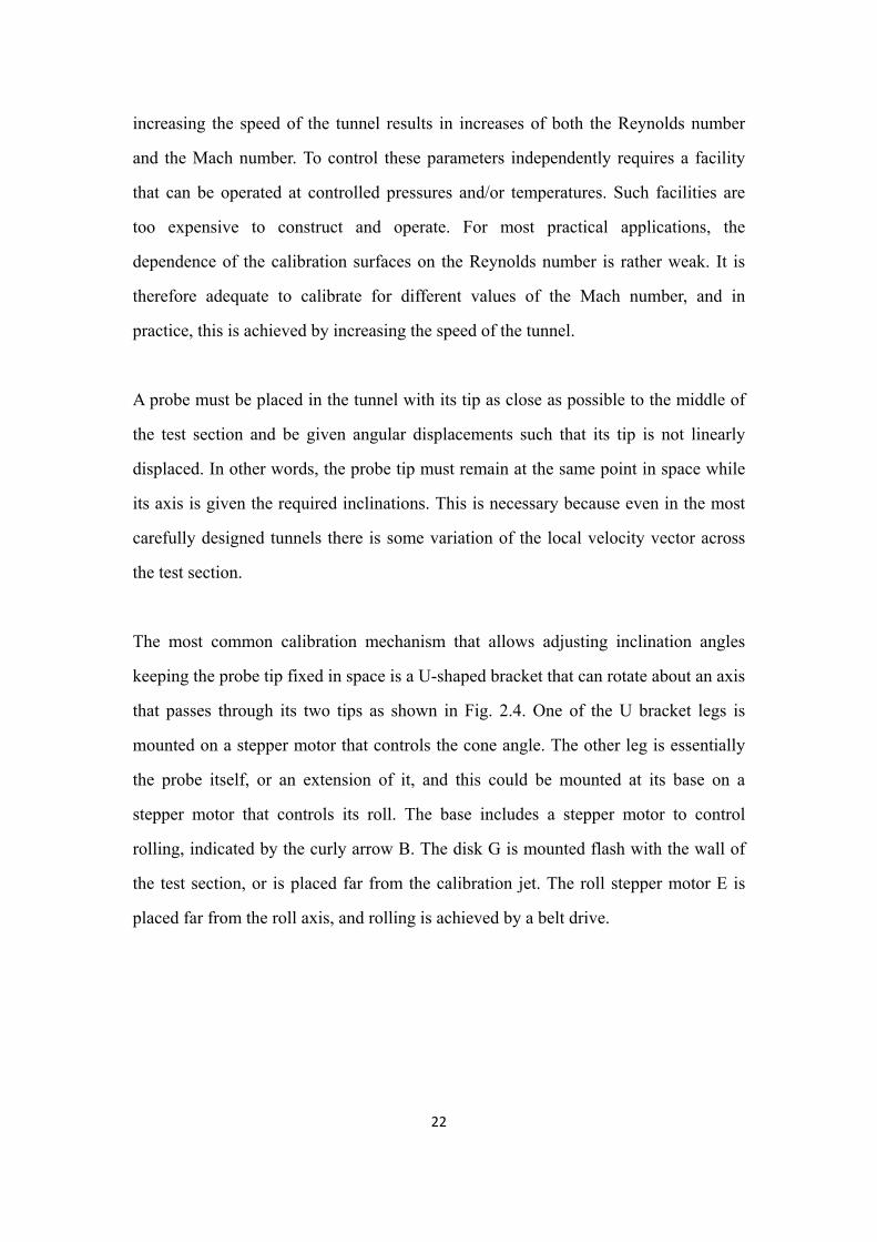
Fig. 2.14 Radial velocity along vertical lines: x/Di= 1 (1” away from stator),  =‐2.9o, ‐5.8 o and ‐8.7 o 

In Fig. 2.14, we show the radial velocities along three vertical lines at different

annular angles ( =-2.9o, -5.8 o and -8.7 o). As we can see, the jet has higher velocity in

the location close to stator blade. Combining with the result in Fig. 2.13, we can draw

the conclusion: the jet stream emerges at the windward corners formed by stator

blades and annular cover of the stator. This is indeed shown clearly in Fig. 2.15, where

radial velocity contours along a plane normal to the radial direction are presented. In

this Figure the vertical and horizontal red lines are radial projections of the stator plate

and the annular roof of the stator.

36   

 

Fig. 2.15 Contour of radial velocity on a vertical plane: x/Di= 1 (1” away from stator) 

 Fig. 2.16 Comparison of the velocity components: x=3”, y/Di=0.622 

In Fig. 2.16, the three velocity components of the jet are compared. The radial velocity

is dominant and the circumferential velocity is almost zero, which implies that the

fluid emerges out of the stator almost radially and horizontally. This can be attributed

to the effect of stator blades and the annular stator cover. Re-directing the stream is

one of the stator’s functions. The circumferential motion of the fluid does not benefit

the machine’s performance, on the other hand, it wastes energy. But this energy is

converted to turbulent energy, a very desirable feature of a flotation machine, since

37   

small-scale turbulence promotes bubble-particle collisions. The longitudinal velocity

is slightly negative. This means the jet is turned downwards and then it makes a

U-turn near the tank wall and finally returns to the bottom of the rotor forming the

lower recirculating toroidal structure. This pattern is consistent with the numerical

results of Fig. 2.11.  

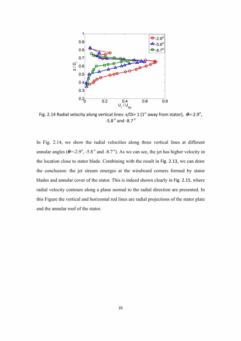
 Fig. 2.17 Ur on Vertical lines: x/Di=1.26 (6” way from stator), angle=‐2.9o   

The returning of the flow is also confirmed by Fig. 2.17. It shows a radial velocity

profile along a vertical line which is 6” away from the stator. The lower part of the

profile is negative. This means that after the fluid is shot out on the upper region, it is

sucked back into the rotor in the lower region due to the pressure gradient generated

by the rotor.

In summary, the fluid is driven out from the impeller region by the rotor inclined

upward and strongly in the circumferential direction. Then the flow impinges on the

stator blade and changes its direction forming a strong jet, which emerges almost

radially. But on the lee side of the stator blades, large inactive flow regions form.

38   

  

Fig. 2.18 Comparison of the three velocity components of returning flow along a vertical line: x/Di=1.26 (6” away from stator),  =2.9o 

  

Fig. 2.19 Comparison of the three velocity components of returning flow along a horizontal line: x/Di=1.26 (6” away from stator), y/Di=0.051 

The returning flow

The five-hole probe was turned 180 degree to investigate the returning flow in the

lower region outside the stator. In Fig.  2.18 and Fig.  2.19, the three velocity

components of the returning flows on vertical and horizontal lines are compared. First,

39   

we observe that unlike the jet stream in the upper region, the velocity of the returning

flow is very uniform spatially. Moreover, we find that all three components of the

velocity are very close to each other in magnitude.

 Fig. 2.20 Radial velocity along horizontal lines x/Di= 1.1 (3” away from stator), 

y/Di=0.622, 0.571, 0.520 

 

 Fig. 2.21 Radial velocity along vertical lines: x/Di= 1.1 (3” away from stator), θ=‐2.9o, 

‐5.8o and ‐8.7o 

 

40   

  

Fig. 2.22 Radial velocity along horizontal lines x/Di= 1.26 (6” away from stator), y/Di=0.622, 0.571, 0.520 

  

Fig. 2.23 Radial velocity along vertical lines: x/Di= 1.26 (6” away from stator), θ=‐2.9o, ‐5.8o and ‐9.2o 

 

Dispersion of the jet stream

To study the dispersion of the jet stream in radial direction, experiments were

conducted on the vertical plane with different x/Di. In Fig. 2.20, Fig. 2.21, Fig. 2.22,

and Fig. 2.23, the radial velocity along horizontal and vertical lines are plotted. We see

that these profiles are very similar to those shown in Fig.  2.13 and Fig.  2.14. The

41   

direction comparison in Fig.  2.24 and Fig.  2.25 shows that as the flow sweeps out

radially, the radial velocity decreases. This is consistent with continuity equations,

since the cross-sectional area of the jet increases with the radial distance. The contour

of the radial velocity as shown in Fig. 2.26 and Fig. 2.27 indicate not only the change of

the velocity magnitude but also the change of jet stream shape. As the jet stream

moves outwards, it slows down and expands. Additionally, the shape of the jet stream

changes from flat to round duo to the free shear layer. The dispersion of the jet stream

increases the active zone of the machine.

 Fig. 2.24 Radial velocity along horizontal lines: x/Di=1, 1.1 and 1.26; y/Di=0.622 

 

 Fig. 2.25 Radial velocity along vertical lines: x/Di=1, 1.1 and 1.26; θ=‐5.8o 

42   

 

 

Fig. 2.26 Contour of radial velocity on a vertical plane: x/Di= 1.10 (3” away from stator) 

 

 

Fig. 2.27 Contour of radial velocity on a vertical plane: x/Di= 1.26 (6” away from stator) 

 

43   

 

Fig. 2.28 Velocity profiles in the quiescent region: x/Di=1.26,  =‐5.8o     

 

Velocity in the quiescent region As described above, when the fluid emerges out from the stator, the radial velocity is

dominant, while the tangential velocity is almost zero, which implies that the fluid

emerges almost radially. The longitudinal velocity is slightly negative, so as the jet

moves further out, it also has a downward trend. Therefore, the jet does not have

direct impact to the fluid above the rotor-stator assembly. The zone above the rotor

stator should be relatively quiescent. The probe was traversed in this region to reveal

the flow pattern characteristics. Since there is no stator and buffer in the quiescent

zone, we can assume that the flow is axially symmetric.

In Fig. 2.28, the three velocity components are compared along a vertical line in the

quiescent region. Here the flow has a slight tangential velocity, which decreases along

the axis. This implies that the circumferential motion is induced from the lower part

of the cell. If the fluid were driven around by the driving shaft, the tangential

velocity should be uniform along z direction. The radial velocity is negative, i.e. the

fluid flows towards the driving shaft from the tank’s wall. The longitudinal velocity is

44   

negative at most of the measuring points, This means that along the measuring line,

the fluid flows from the top to bottom. These results confirm the existence of a second

toroidal structure on the upper part of the cell. The two toroidal structures have

opposite sense of rotation.

 

Fig. 2.29 Comparison of velocity profiles in pilot and commercial cells 

 

Comparison of the velocity profiles in different cells

The jet described above was detected in a commercial cell as well, as shown in Fig. 

2.29, where we present velocity measurements obtained with a five-hole probe in two

facilities. The jet in the commercial cell is a little more narrow but just as strong. The

results from the pilot cell and commercial cell match reasonably well, even though the

corresponding Reynolds numbers were quite apart, namely, for the pilot and the full

size cell, Re=1.2×105 and 3.3×106 respectively.

2.5 Summary We employed the standard five-hole probe to the large scale stirring tank

measurements. There are many advanced technologies and instruments for

hydrodynamics measurement, such as Particle Image Velocimetry (PIV) and Laser

0

0.05

0.1

0.15

0.2

0.25

-0.2 0 0.2 0.4 0.6 0.8u/utip

y/D

pilot cell

commercial cell

45   

Doppler Velocimetry (LDV). However these tools are only practical in

well-controlled laboratory environments, since they need very good optical access.

The five-hole probe has been proved to be a robust, reliable and cost-efficient method

for stirring tank hydrodynamics investigation.

The results indicate that the flow in a flotation cell is driven by a jet issuing radially

from the very top of the impeller. There is a substantial circumferential component in

this jet, a fact well expected, since it is produced by rotating flat blades. But when the

jet emerges from the stator the circumferential component is drastically reduced. It is

due to the circumferential component that the stator plates generate regions of

separated flow, which give rise to large-scale turbulence. Large-scale turbulent

structures require considerable distances to break down to smaller scales. It is the

small-scale turbulence that is required to break down bubbles, which in turn can

capture and float particles.

The radial jet that emanates from the upper part of the impeller emerges out of the

stator in almost the radial direction. But it deflects in anticipation of its encounter with

the tank side walls. Two toroidal regions form, which are isolated from each other.

The low toroidal motion is driven directly by the jet. The upper region must be driven

by shearing along the interface of the two regions. Mixing between these regions is

due only to the turbulent shearing interface between them. As a result, the top region

is almost quiescent, while the bottom is violently agitated.

46   

References 1. Abrahamson, J., Collision rates of small particles in a vigorously turbulent

fluid. Chemical Engineering Science, 1975. 30: p. 1371-1379.

2. Koh, P.T.L., M. Manickan, and M.P. Schwarz, CFD simulation of

bubble-particle collisions in mineral flotation cells. Mineral Engineering,

2000. 13: p. 1455-1463.

3. Koh, P.T.L. and Schwarz M.P., CFD modeling of bubble-particle attachments

in flotation cells. Minerals Engineering, 2005. 19: p. 619-626.

4. Koh, P.T.L. and M.P. Schwarz, CFD Modeling of Bubble-Particle Collision

Rates and Efficiencies in a Flotation Cell. Minerals Engineering, 2003. 16: p.

1055-1059.

5. Brucato, A., et al., Numerical Prediction of Flow Fields in Baffled Stirred

Vessels: A Comparison of Alternative Modeling Approaches. Chem. Eng. Sci.,

1998. 53: p. 3653-3684.

6. Mavros, P., Flow Visualization in Stirred Vessels: A Review of Experimental

Techniques. Trans IChemE, 2001. 79: p. 113-127.

7. Rao, M.A. and R.S. Brodkey, Continuous Flow Stirred Tank Turbulence

Parameters in the Impeller Stream. Chem. Eng. Sci., 1972. 27: p. 137-156.

8. Wu, H. and G.K. Patterson, Laser-Doppler Measurements of Turbulent-Flow

Parameters in a Stirred Mixer. Chem. Eng. Sci., 1989. 44: p. 2207-2221.

9. Schafer, M., M. Hofken, and F. Durst, Detailed LDV Measurements For

Visualization of The Flow Field Within A Stirred-Tank Reactor Equipped With

A Ruston Turbine. Trans IChemE, 1997. 75: p. 729-736.

10. Gaskey, S., et al., A method for the study of turbulent mixing using

Fluorescence spectroscopy. Exper. In Fluids., 1990. 9: p. 137-147.

11. Law, A.W.K. and Wang H., Measurement of Mixing Processes With Combined

Digital Particle Image Velocimetry and Planar Laser Induced Fluorescence.

Experimental Thermal and Fluid Science, 2000. 22: p. 213-229.

47  

Chapter 3 Multi-phase Flow Characterization

Instrumentation is available to obtain samples and then measure the local void

fraction as well as the size and number density of bubbles and/or particles in two and

three-phase flow. But in most cases, these methods interfere with the flow and bias

the sampling process. We have developed an isokinetic sampling probe system that

can take accurate samples without changing the sample’s composites. This is achieved

by aligning the probe’s intake nozzle with the flow’s local predominant direction and

matching its internal pressure with its hydrodynamic environment and hence equalize

the inside and outside velocities. Then the fluid sample’s density is measured to

calculate the local void fraction. The calibration procedure and results as well as the

extensive test data obtained in bubbly-flow tunnels and flotation cells are presented

and discussed in this Chapter. The isokinetic sampling probe system was employed in

Dorr-Oliver tanks to evaluate its air dispersion capability.

3.1 Introduction

In a typical flotation machine, the strong turbulent flow generated by the rotor breaks

large air bubbles into small bubbles and disperses them to the whole tank. At the same

time, particles are also dispersed and suspended into the tank by the turbulent flow.

Bubble-particle collision, attachment and detachment then occur. It has been widely

acknowledged that the flotation recovery rate depends on a wide range of complex

factors. One of the most important factors is the gas dispersion characteristics of the

flotation cell. Gas dispersion characteristics include bubble size (Sauter mean

diameter d32), superficial gas velocity (Jg), gas holdup and the derived quantity bubble

surface area flux (Sb=6Jg/d32). All of these properties are known to have direct

influence on the flotation efficiency.

Gas holdup ( ) is defined as the fraction occupied by the gas phase in the total volume

of two- or three-phase mixture.

48  

100% (3.1)

The term “gas holdup” is well established in the mining engineering community. A

more common term for the same quantity is “void fraction”. We will use the first term

if it was chosen by the authors of papers describing equipment employed in flotation

machines. To study the impact of the multi-phase flow characteristics on the tanks’

performances, it is necessary to obtain and analyze the true local samples in two- and

three-phase flow. A few invasive and non-invasive techniques have been developed

by scientists and engineers for research and industrial applications as reviewed by

Boyer et al [1]. Fig. 3.1 shows the sketch of a typical gas holdup meter. It consists of a

graduate container with two open ends, two flip covers and the pneumatic actuator

system. During the measurement procedure, the gas holdup meter is sunk down to the

target region with the flip covers open. After the cylinder is filled up by the local

fluid, the pneumatic actuators are activated to shut the covers on both ends. After the

local fluid sample is taken, the whole device is pulled out of the pulp. The gas holdup

can then be read directly from the scale on the container wall. This gas holdup meter

is simple and can measure the local void fraction and particle concentration directly.

However, it is too big, which results in very low spatial resolution. A more serious

problem is that it disturbs the local flow due to its large size, and hence cannot obtain

accurate multi-phase fluid samples.

 

Fig. 3.1 Sketch of gas holdup meter 

 

49  

Gomz and Finch measured the gas dispersion in flotation cells using a gas-holdup

sensor, which is based on conductivity[2]. A typical conductivity probe is a hollow

plastic tube with two electrodes arranged inside axially. As the name implies, the

electrodes measure the conductivity of the fluid flowing through the tube.

Pre-calibration is conducted in multi-phase flow to establish the relationship between

the conductivity rate of the fluid and the void fraction. Comparing with the gas holdup

meter, the conductivity probe is much smaller and its operation can be automated.

However, the calibration procedure is very complicated. Another shortage of this

device is that it is not able to obtain true samples without changing the fluid

characteristics.

The McGill Viewer (or McGill bubble size analyzer) tool is another established tool

in industry. It consists of a peristaltic pump and a PVC tube. The bubbles rise along

the tube and are guided into an inclined chamber. Once in the chamber, the bubbles

float up and enter the upper side of the inclined window of the chamber, where a

digital camera is set to capture the bubble images. Digital imaging processing

technology is used to measure the bubbles’ diameters and determine the bubble size

distribution, from which the Sauter mean diameter is calculated[3, 4].

The McGill tool is a widely-used device in industry, but this tool discriminates in its

sampling and it is hard to move from point to point in the domain of interest.

Moreover, allowing for bubbles and bubble/particle aggregates to rise over long

elevations to the measuring location induces changes on the sample that cannot be

accounted for. Additionally, the McGill tool would fail entirely if it is inserted in the

highly activated domains of a flotation machine, namely in the immediate

neighborhood of the impeller and the stator. But this is where most of the important

flotation processes are taking place, and where our observations and measurements

should be concentrated. Another limitation involves cleaning the viewing chamber.

As bubbles loaded with solid particles rise to the top of the viewing chamber, they

burst and release the solid particles, which accumulate in the chamber and reduce the

quality of the images.

50  

A typical industry method for air holdup measurement is taking samples by sucking

flow out from the bulk[5]. However, if the flow is not sampled under isokinetic

condition, it leads to obvious errors. Many people have stated that the aerated media

must be withdrawn under isokinetic conditions, which means the multi-phase flow

should be sucked in with the same speed as it approaches the sampling probe[6, 7].

Isokinetic sampling probes are a kind of devices that have wide applications in

multi-phase flow environments [8-10]. The isokinetic sampling probe working

principle is described in section 3.2.

In this Chapter we describe the development of instrumentation appropriate for

exploring multi-phase flow in complex turbulent flows. The main consideration is to

obtain samples without disturbing the local flow. The instruments developed provide

information on the local value of the void fraction and the velocity components of the

flow. We then describe the experiments conducted in flotation cells, present the

results and discuss their significance.

3.2 Instrument development

3.2.1 Development of Isokinetic Sampling Probe (ISP)

Isokinetic sampling probes have been described in the literature[8-10]. But in all these

cases the alignment of the probe does not present a problem, because these probes

were employed in pipe flows or other situations where the direction of the flow is

known. In the problems we need to explore here the flow is very complex and the

direction of the flow is not known. This requires that a method must be devised to

align the probe with the local direction of the velocity vector. Another requirement is

that the flow velocities inside and outside the probe should be the same. We devised a

method that could guide the operator to make these adjustments to achieve accurate

measurements.

 

 

To

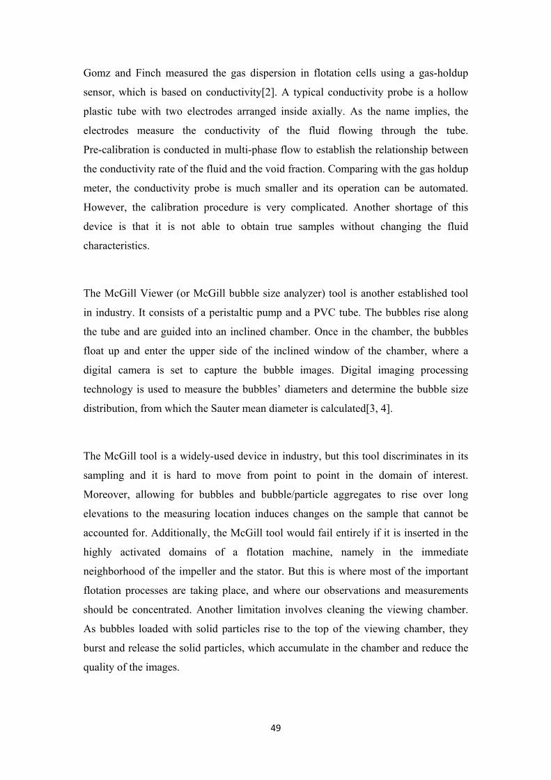
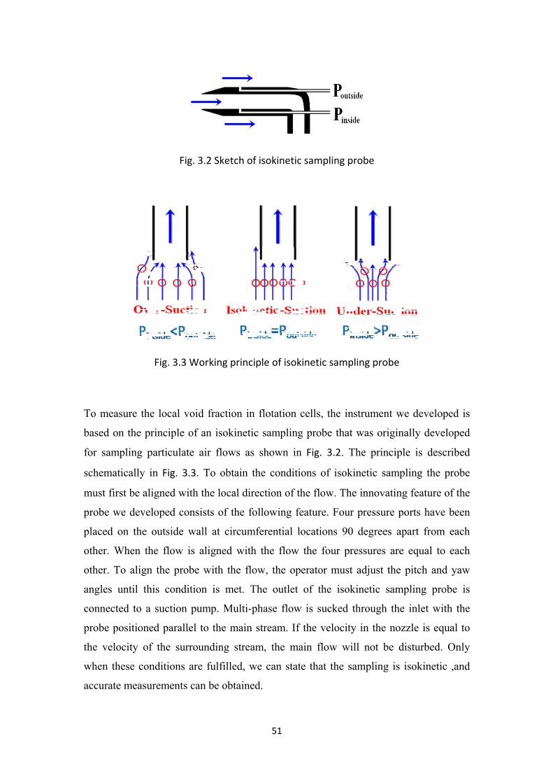
base

for

sche

mus

prob

plac

othe

othe

ang

conn

prob

the

whe

accu

measure th

ed on the p

sampling p

ematically i

st first be al

be we deve

ced on the

er. When th

er. To align

les until th

nected to a

be positione

velocity of

en these con

urate measu

Fig. 3

Fig. 3.3 Wo

e local void

principle of

particulate a

in Fig. 3.3.

ligned with

eloped consi

outside wa

he flow is a

n the probe

his conditio

a suction pu

ed parallel

f the surrou

nditions are

urements ca

3.2 Sketch o

orking princ

d fraction in

an isokinet

air flows a

To obtain

the local di

ists of the f

all at circum

aligned wit

with the fl

on is met.

ump. Multi-

to the main

unding stre

e fulfilled, w

an be obtain

51 

of isokinetic

ciple of isok

n flotation

tic sampling

as shown in

the conditi

irection of t

following fe

mferential l

th the flow

low, the op

The outlet

-phase flow

n stream. If

am, the ma

we can stat

ed.

c sampling p

kinetic samp

cells, the in

g probe that

n Fig.  3.2. T

ions of isok

he flow. Th

feature. Fou

locations 90

the four p

perator must

of the iso

w is sucked

f the velocit

ain flow w

te that the s

 

probe 

pling probe 

nstrument w

t was origin

The princip

kinetic samp

he innovatin

ur pressure p

0 degrees a

ressures are

t adjust the

kinetic sam

through th

ty in the no

will not be d

sampling is

 

 

we develope

nally develo

ple is descr

pling the p

ng feature o

ports have b

apart from

e equal to

e pitch and

mpling prob

e inlet with

ozzle is equ

disturbed. O

isokinetic

ed is

oped

ribed

robe

f the

been

each

each

yaw

be is

h the

al to

Only

,and

52  

In sampling bubbly flow, over-suction gives higher void fraction readings while

under-suction gives lower readings. In water-particle flow, the opposite is true:

over-suction results in lower particle concentration readings while under- suction

results in higher readings. Pressures are also measured on the inside and the outside

wall of the probe as shown in Fig. 3.2 . The velocity inside the probe is equal to the

velocity outside the probe if these two pressures are equal. This is achieved by

adjusting the suction rate on the probe.

 

Fig. 3.4 Isokinetic sampling probe 

One of the isokinetc sampling probes we developed is shown Fig. 3.4. It has a pressure

port inside to measure the insider static pressure. Four pressure ports are arranged on

the stem along the circumferential direction to measure the outside static pressure.

Two of these ports are shown in the Figure. The four pressure ports are also used to

adjust the direction of the isokinetic sampling probe. Once pressures in the four ports

are equal, the probe is aligned with the local flow.

3.2.2 Flow visualization of the isokinetic sampling probe

To confirm the working principle described above (Fig. 3.3), two-dimensional flow

visualization experiments were set up and run. The experimental layout is shown in 

Fig. 3.5. Two pieces of Plexiglas plates were placed parallel to each other to form a

two-dimensional channel. This channel was set in the middle of a closed circuit

which includes tubes, valves and pump. A sparger was set near the channel’s inlet

to generate air bubbles. This system can generate uniform two-dimensional bubbly

flow. A two-dimensional isokinetic sampling probe was fabricated and installed in

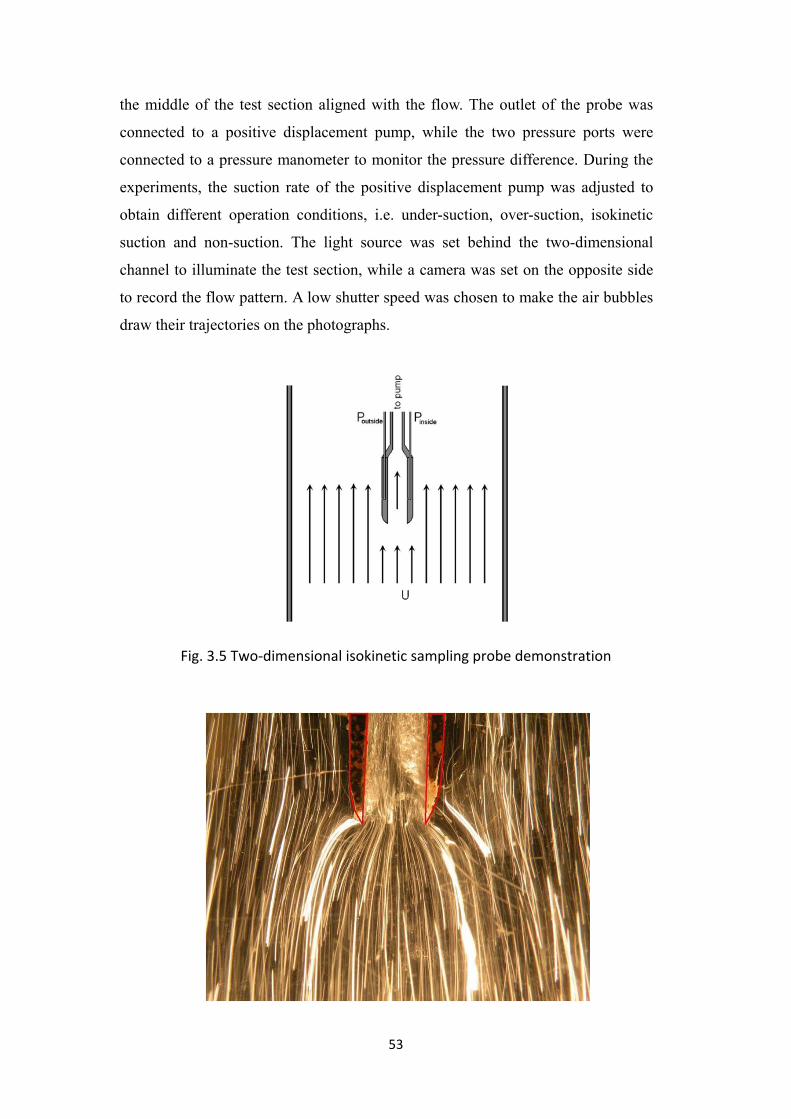
53  

the middle of the test section aligned with the flow. The outlet of the probe was

connected to a positive displacement pump, while the two pressure ports were

connected to a pressure manometer to monitor the pressure difference. During the

experiments, the suction rate of the positive displacement pump was adjusted to

obtain different operation conditions, i.e. under-suction, over-suction, isokinetic

suction and non-suction. The light source was set behind the two-dimensional

channel to illuminate the test section, while a camera was set on the opposite side

to record the flow pattern. A low shutter speed was chosen to make the air bubbles

draw their trajectories on the photographs.

 

Fig. 3.5 Two‐dimensional isokinetic sampling probe demonstration

 

54  

Over-suction

Under-suction

Non-Suction

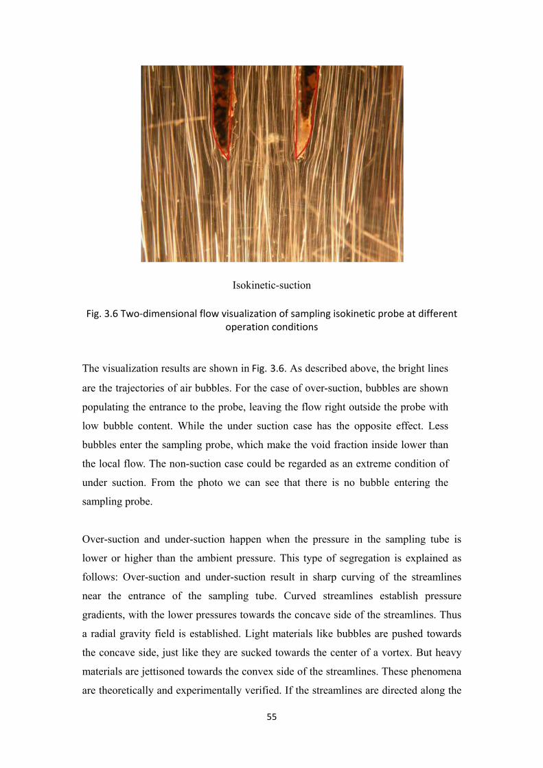
55  

Isokinetic-suction

Fig. 3.6 Two‐dimensional flow visualization of sampling isokinetic probe at different operation conditions

The visualization results are shown in Fig. 3.6. As described above, the bright lines

are the trajectories of air bubbles. For the case of over-suction, bubbles are shown

populating the entrance to the probe, leaving the flow right outside the probe with

low bubble content. While the under suction case has the opposite effect. Less

bubbles enter the sampling probe, which make the void fraction inside lower than

the local flow. The non-suction case could be regarded as an extreme condition of

under suction. From the photo we can see that there is no bubble entering the

sampling probe.

Over-suction and under-suction happen when the pressure in the sampling tube is

lower or higher than the ambient pressure. This type of segregation is explained as

follows: Over-suction and under-suction result in sharp curving of the streamlines

near the entrance of the sampling tube. Curved streamlines establish pressure

gradients, with the lower pressures towards the concave side of the streamlines. Thus

a radial gravity field is established. Light materials like bubbles are pushed towards

the concave side, just like they are sucked towards the center of a vortex. But heavy

materials are jettisoned towards the convex side of the streamlines. These phenomena

are theoretically and experimentally verified. If the streamlines are directed along the

56  

axis of the tube with no curving, then there will be no discrimination of light or heavy

materials that are transported with the flow. These conditions can be achieved first by

aligning the probe with the flow, and then securing that the pressure inside the tube is

the same with the pressure outside the tube.  

3.2.3 Void fraction analyzer

Working Principle

 

One of the multi-phase flow properties of interest that can be obtained by

isokinetic sampling is the local void fraction. To determine the local void fraction,

we devised the system shown in Fig.  3.7, which was designed, constructed and

tested. Driven by a pump with adjustable head, the pulp fluid passes along an

ascending and a descending part of a tube, and the static pressures are measured at

four pressure ports. Pressure differences can then return the air fraction according

to the following derivation which is based on the energy equation.

                                                                                  (3.2) 

                                                                                  (3.3) 

2                                                                           (3.4) 

                                                                                              (3.5) 

1

                                                  (3.6) 

 

Here cpc is the presure correction coefficent, which will be discussed in the next

paragraph. Note that with a constant inner diameter of the pipe, the velocity does

not vary along the length of the tube, and thus these relationships are just

hydrostatic. In this design, wall friction is compensated using the two sections of

the pipe, namely the ascending and descending sections where the flow is first

opposite to and then points in the direction of gravity. This device can collect data

57  

automatically, and works for both two-phase flow and three-phase flow.

 

Fig. 3.7 Local void fraction measurement system based on Isokinetic sampling probe 

 

 

Fig. 3.8 Layout of the system for local void fraction and solid concentration measurements 

It is essentially a densitometer that can operate on line with the fluid flow. It is not

necessary to carry out static measurements. One such densitometer module is

needed for two-phase flow. But a design modification can be used to obtain both

void fraction and particle concentration. Here is a proposal, for an instrument that

58  

has not been constructed yet. Two modules are needed (Fig.  3.8). The first one

measures the three-phase flow density, namely ρ , and then a hydraulic

cyclone or other separator can be used to remove air. The second measures the

water-particle two-phase flow density, ρ . Hence, in a unit volume, the fractions

of water, particle and air are derived as follows:

1 (3.7)

(3.8)

Pressure Correction due to Elevation Differences

 

The isokinetic sampling system can obtain the true sample from the target region.

However, when the analysis is performance, the characteristics of the sample may

change due to the difference of elevation between the sampling and the measurement

points For the water-air two-phase flow in our case, a true sample is taken from the

flotation tank, but the static pressure changes with the elevation of the measurement

location, which results in air volume change, i.e., the void fraction of the sample is not

the same as in the tank. Since the static pressure is always monitored and recorded

during the test, the pressure correction coefficient cpc can be obtained.

(3.9)

(3.10)

Here is the absolute static pressure before the sample is taken while is the

average absolute static pressure in the analyzer system and = (p1+p2+p3+p4)/4.

and are the temperature of the sample before and after it is taken out. Here

we assume = . A sample calculation is given here to show the influence of

pressure change in the tests.

59  

At a typical test condition in the 6m3 Dorr-Oliver tank, is 107588 Pa while

varies from 104500 Pa to 109500 Pa. So ranges from 0.971 to 1.018. This means

that without the pressure correction, there will be an error between -2.9% and 1.8%.

Uncertainty analysis for the void fraction measurements

 

The local void fraction calculation is based on pressure measurements as shown in Eq.

3.6. According to the error propagation principle, the uncertainty of the local void

fraction can be written as the follow.

                                                        (3.11) 

                                  (3.12) 

2 100%                                                                                              (3.13) 

Here is the uncertainty of the pressure transducer. As we can see, the uncertainty of

the void fraction measurement is directly related to the uncertainty of the pressure

sensors. The error associated with the pressure sensor used in the experiments is

±0.25% of the full scale.

3.2.4 Experimental facilities and isokinetic sampling probe

calibration

To test and calibrate the isokinetic sampling probe system, a vertical bubbly flow

tunnel and a horizontal high speed multi-phase jet tunnel were designed and built in

the ESM fluids laboratory (Fig. 3.9 and Fig. 3.10). These facilities can generate bubbly

flows with known and repeatable laboratory conditions.

60  

 

Fig. 3.9 Vertical multi‐phase flow tunnel 

 

Fig. 3.10 High speed multi‐phase jet tunnel 

The vertical bubbly flow tunnel consists of a 50 gallon plastic container, a 1/4 horse

power submersible pump, a 2” ID transparent pipe, a sparger system, tubing system,

some valves and some other accessories. Water is pumped into the sparger chamber

through 2” PVC pipes. Air is injected into the sparger, which is a pipe rake made of

porous materials, to generate bubbles. The bubbles mix with water in the chamber. A

honeycomb plate is installed in the inlet of the vertical test section to generate uniform

flow. The test section is 2” in diameter and 4’in length. After passing through the test

section pipe, the flow returns to the container and the bubbles are released at the water

free surface in the quiescent environment. A surfactant, MIBC, is mixed with water to

61  

control the size of the bubbles by adjusting the MIBC concentration. The liquid flow

meter and a gas flow meter are used to measure the flow rate of the two phases before

they mix. From the readings of the flow meters, we can calculate the average void

fraction in the test section. By adjusting the gas flow rate, we can get different void

fractions.

The high-speed jet tunnel was designed to be versatile. It can operate in single-phase

flow and multi-phase flow conditions. It consists of a rectangular tank, tubing system,

a centrifugal pump, a T-shaped separating plate, a sponge, a sparger, a honeycomb

structure, some valves and some other accessories. The tank is 22”wide x 65” long x

20” deep. The centrifugal pump is powered by a 3-horsepower electric motor and its

maximum pumping capacity is 120 gallon/minute. The diameter of the jet tunnel

nozzle can be set as 2”, 1.5” or 1”. A honeycomb plate is installed ahead the nozzle to

generate uniform flow. The tubing system consists of 2” PVC pipes. A turbine flow

meter (Great Plains A1 Turbine Flow Meter) is set between pipes to monitor the flow

rate. The measuring range is 0.3 to 300 gallon/minute. The T-shaped separating plate

and sparger will be used only in two- and three-phase flow. For two-phase flow, air is

injected into the sparger to generate small bubbles. The surfactant, MIBC, is added to

control the bubble size. A gas flow meter is used to measure the gas flow rate.

Combing the liquid flow rate and the gas flow rate, we can calculate the air fraction of

the jet flow. When the flow returns from the nozzle side to the pump side, it overflows

from the T plate, the bubbles rise and escape at the free surface. A sponge is put on

the top of the T plate to remove smaller bubbles. Hence what is sucked into the pump

is always single-phase fluid. This facility can also run in three-phase flow condition

by feeding particles into the pump inlet at a constant rate. As with the three-phase

flow operation, no particles can escape from the nozzle side to the pump side. Since

the motor speed cannot be adjusted, the jet speed is controlled by adjusting the valves

in the piping system.

Since the high-speed jet tunnel can be run in both single-phase flow and multi-phase

flow conditions, it can be used to simulate the flows found in the high-speed domains

of flotation machines. This would be adequate for the testing and calibration needs,

but this facility does not offer optical access to the domain of interest. Such access is

62  

available in the vertical bubbly-flow tunnel. Moreover, by controlling the air flow rate

and surfactant concentration, we can generate in the vertical bubbly-flow tunnel much

larger bubbles that are common in flotation machines.

The isokinetic sampling probe and the densitomer were tested in the ESM Fluids

Lab. The isokinetic sampling probe was aligned with the flow in both the vertical

bubbly flow tunnel and horizontal high speed jet tunnel. Air and water supply rates

were measured by independent flow meters. In terms of these quantities we

calculate the void fraction and present it in Table 3.1 and Fig. 3.11 as calculated

void fraction. The measurements obtained by the isokinetic densitometer are

defined as measured void fraction. The results show that the isokinetic system

provides accurate measurements with excellent repeatability. The deviation is less

than 2%.

To show how important the isokinetic sampling condition is to the void fraction

measurement, some tests were conducted under non-isokinetic conditions. The

effect of the suction rate and inclined angle were examined. Fig. 3.12 and Fig. 3.13 

show that the errors in proper setting of suction rate and alignment results in

serious measurement errors. For the under-suction case, the reading of local void

fraction is also lower, because less number of bubbles get into the isokinetic

sampling probe as discussed in 3.2.2. While for the over-suction case, we always

get higher readings. Errors in the probe alignment always return higher readings.

Fig.  3.12 and Fig.  3.13 indicate that it is very important to align the probe and

match the suction rate in the tests. However, from the plots we can see that minor

departures in alignment and suction rates do not affect the reading very much.

63  

 

Table 3.1 Isokinetic sampling probe system validation 

 

 

Fig. 3.11 Validation of the Isokinetic sampling probe system 

 

64  

 

Fig. 3.12 Influence of suction rate on void fraction measurement: y/Di=‐0.071, z/ Di =0.653, MIBC= 21ppm, Qair= 2.63 m

3/min and Utip=6.4 m/s 

 

 

Fig. 3.13 Influence of the probe inclined angle on void fraction: y/Di=‐0.071, z/ Di =‐0.653, MIBC=21 ppm, Qair= 2.63 m

3/min, Utip=6.4 m/s 

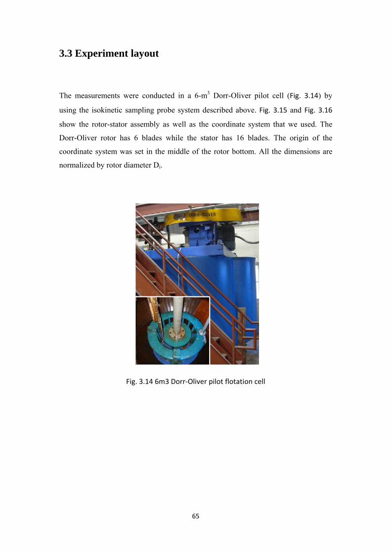
65  

3.3 Experiment layout

 

The measurements were conducted in a 6-m3 Dorr-Oliver pilot cell (Fig.  3.14) by

using the isokinetic sampling probe system described above. Fig. 3.15 and Fig. 3.16

show the rotor-stator assembly as well as the coordinate system that we used. The

Dorr-Oliver rotor has 6 blades while the stator has 16 blades. The origin of the

coordinate system was set in the middle of the rotor bottom. All the dimensions are

normalized by rotor diameter Di.

 

Fig. 3.14 6m3 Dorr‐Oliver pilot flotation cell 

 

66  

 

Fig. 3.15 Sketch of Dorr‐Oliver tank rotor‐stator assembly (side view) 

 

 

Fig. 3.16 Sketch of Dorr‐Oliver tank rotor‐stator assembly (top view) 

 

Two steps are required before samples can be obtained using the isokinetic

sampling probe. First the probe axis must be aligned with the local direction of the

flow. Then the suction velocity must be matched with the local flow. Both steps

are guided by pressure measurements. Four pressure taps are placed on the outside

of the probe tube, positioned meridionally 90 degrees apart, and at a distance of a

few diameters from the probe nozzle. Aligning the probe with the flow requires

that the pressure at the four ports is equal to each other. Once alignment is

achieved, then the suction level must be adjusted. Now two pressure measurements

are needed, one on the inside wall of the probe and another on the outside wall, as

shown in Fig.  3.2. Since the flow is aligned with the flow, matching the inside

 

pres

outs

alig

in F

gim

By

thro

out

are

3.4

The

in th

Loc

The

roto

ssure with t

side velocit

gnment with

Fig. 3.17. Th

mbal mechan

twisting the

ough a flexi

manually, b

needed.

4 Local v

e tools deve

he 6-m3 Dor

cal void fra

e probe was

or’s tip velo

the outside

ty and isok

h the flow, t

his mechani

nism is bolt

e pole, the y

ible drive sh

but automa

void frac

loped and d

rr-Oliver pi

action for d

s set in the

ocity was se

pressure in

kinetic cond

the probe is

ism can adju

ted to a pol

yaw angle c

haft and thr

ation is also

Fig. 3.17

ction me

described ab

ilot flotation

ifferent air

jet region

et at 6.4 m/

67 

nsures that

ditions have

s mounted o

ust the pitch

le which is

can be adju

read. Curren

o practical i

7 Gimbal me

asureme

bove were e

n machine.

r flow rate

at x=1.260D

/s and the c

the inside

e been ach

on a gimba

h and yaw a

mounted to

usted. The p

ntly all thes

f a large nu

echanism 

ents resu

employed in

Di, y=-0.07

concentratio

velocity is

ieved. To f

al mechanism

angles of th

o the traver

pitch angle

se processe

umber of m

ults and

n measurem

71 Di and z

on of the su

equal to th

facilitate th

m, as show

he probe. Th

rsing system

is controlle

es are carrie

measurement

 

discussio

ments condu

z=0.653 Di.

urfactant M

he

he

wn

he

m.

ed

ed

ts

ons

ucted

The

MIBC

68  

was 14ppm, while the air pumping flow rate was varied to study its influence on the

local void fraction. In Fig. 3.18 we present the local void fraction measured in the jet

region as a function of the air flow rate supplied to the machine. As we can see, the

relationship is linear, indicating that at the point of measurement, the local void

fraction is directly related to the supplied air flow rate.

 

Fig. 3.18 Void fraction for different air flow rates: Utip=6.4 m/s, MIBC=14 ppm, y/Di=‐0.071, z/ Di =0.653 

 

Local void fraction for different tip velocity

The probe was set in the jet region at x=1.260Di, y=-0.071 Di and z=0.653 Di. The air

pumping flow rate was set at 2.63 m3/min and the concentration of the surfactant

MIBC was 14ppm, while the rotor’s tip velocity was varied to study its influence on

the local void fraction. Fig. 3.19 presents measured void fraction for varying blade tip

velocities with fixed air rates. It is interesting to see that when the rotor’s tip velocity

is lower than 3m/s, almost no air reached the point of measurement. Apparently

buoyancy drives the air up through the rotor-stator gap immediately after it emerges

out from rotor. As the rotor’s tip velocity increases, we now see that for low tip

velocities, the void fraction increases almost linearly, but this trend changes and the

increases are gradual, until at high tip velocities, there is very small influence of this

69  

quantity on the void fraction. This indicates that increasing the speed further will not

be accompanied with higher void fractions, which means for the air dispersion

purpose, this level of tip speeds and the corresponding power input are optimal. It is

possible that at high speeds, air is dispersed in a wider area and is not captured by our

probe at the specific location of x=1.260Di, y=-0.071 Di and z=0.653 Di.

 

Fig. 3.19 Void fraction for different tip velocities: Qair=2.63 m3/min, MIBC=14 ppm, 

y/Di=‐0.071, z/ Di =0.653 

 

Local void fraction for different surfactant concentration

 

The probe was set in the jet region at x=1.260Di, y=-0.071 Di and z=0.653 Di. The air

pumping flow rate was set at 2.63 m3/min and the rotor’s tip velocity was set at 6.4

m/s while the concentration of the surfactant-MIBC- was varied to study its influence

on the local void fraction. The results shown in Fig. 3.20 indicate that MIBC mixtures

not only affect the size of the bubbles but also dramatically affect the void fraction.

As the MIBC concentration is increased, smaller bubbles are generated, which follow

the stream better and yield higher void fraction at the measuring point.

 

70  

 

Fig. 3.20 Void fraction for different MIBC concentrations: Utip=6.4 m/s, Qair=2.63 m3/min, y/Di=‐0.071, z/ Di =0.653 

 

Local Void fraction distribution along horizontal lines

Local void fractions at different elevations were obtained in the 6-m3 machine as

shown in Fig. 3.21. These measurements were obtained by traversing the probe along

a horizontal line covering the space downstream of a stator. The point θ=0 is along the

radial extension of a stator blade. Positive angle values mean that the probe is in the

downstream of the separated region of the stator blade (leeward side), and negative

values is the attached flow side, namely the windward side. The results indicate that

the air is dispersed on the both the active and the inactive zones. The jet region has

relatively high local void fraction since the air bubbles are brought out by the jet

stream. However, the void fraction distribution is pretty uniform along the horizontal

lines. The local void fraction in the dead zone is only around 10% less than the jet

region.

71  

 

Fig. 3.21 Local void fraction on horizontal lines: Utip=6.4 m/s, Qair=2.63 m3/min, x/ Di 

=1.26, MIBC=14ppm 

 

 

Fig. 3.22 Local void fraction on vertical lines: Utip=6.4 m/s, Qair=2.63 m3/min, x/ Di 

=1.26, y/ Di =‐0.071, MIBC=14ppm 

 

72  

Local void fraction along vertical lines

In Fig. 3.22, void faction measurements are presented obtained along a vertical line

crossing the jet where y/Di=-0.071. This Figure indicates that the void fraction

increases with the depth. Apparently buoyancy of very small bubbles is very small,

and their tendency to rise is overcome by the convective action of the stream, even in

the regions where the flow velocity is small.

 

Fig. 3.23 Comparison of global air holdup and local void fraction for different air flow rate: Utip=6.4 m/s 

Comparison of local void fraction and the global air holdup

 

The isokinetic sampling probe was set in the jet (y/Di=-0.071, z/ Di =-0.653) to

measure the local void fraction under different operation condition. At the same time,

the rising level of the water free surface was measured to calculate the global air

holdup. In Fig. 3.23, the rotor tip velocity was set as 6.4 m/s while the air flow rate

varied. The results show that the global air holdup is always higher than the local void

fraction in the jet region. This confirmed our previous conclusion: the highest local

73  

void fraction is noT in the jet region. Moreover, we observe that the local value of the

void fraction in the jet region follows consistently the global value of air hold up.

 

3.5 Summary

 

An isokinetic sampling system was invented for multi-phase flow characterization.

The isokinetic probe has a pressure port inside to measure the inside static pressure.

Four pressure ports are arranged on the stem on the circumferential direction to

measure the outside static pressure. The four pressure ports are used to align the probe

with the local flow by detecting the flow direction, which is the unique feature of the

device.

This isokientic probe system was used to take true samples in the bubbly flow in a

flotation tank.The samples were then analyzed to obtain the local void fraction

continuously. The system can also be extended to conduct local solid concentration

measurements. Local void fraction measurements show that the air bubbles are carried

by the stream and dispersed to the bulk uniformly, even in the inactive zone. The local

void fraction measurement provides the information to evaluate the air dispersion

ability of the tank. It also provides the flow density information, which is used for

velocity measurement by using multi-hole probes.

74  

References

1. Boyer, C., Duquenne, A.-M., Wild, G., Measuring techniques in gas–liquid

and gas–liquid–solid reactors. Chemical Engineering Science, 2002. 57(16):

p. 3185-3215.

2. Gomez, C.O., Finch, J. A., Gas diserprsion measurements in flotation cells.

International Journal of Mineral Processing, 2007. 84: p. 51-58.

3. Gomez, C.O. and J.A. Finch, Gas dispersion measurements in flotation cells.

Int. J. Miner. Process, 2007. 84: p. 51-58.

4. Nesset, J.E., et al., Some gas dispersion characteristics of mechanical flotation

machines. Minerals Engineering, 2006. 19: p. 807-815.

5. Schwarz, S., Alexander, D., Gas dispersion measurements in industrial

flotation cells. Minerals Engineering, 2006. 19: p. 554-560.

6. Greaves, M., Kobbacy, K., Measurement of bubble size distribution in

turbulent gas-liquid dispersion. Chemical Engineering Research and Design,

1984. 62: p. 3-12.

7. Sherwood, J.D., Bubble collection by a point sink in a uniform flow.

International Journal of Multiphase Flow, 2003. 29: p. 621-627.

8. Boothroyd, R.G., An anemometric isokinetic sampling probe for aerosols.

Journal of Scientific Instruments, 1967. 44: p. 249-253.

9. Zhang, G.J., Ishii, M., Isokinetic sampling probe and image processing

systems for droplet size measurement in two-phase flow. International Journal

of Heat and Mass Transfer 1995. 38(11): p. 2019-2027.

10. Dennis, R., Samples, W. R., Anderson, D. M., Silverman, L., Isokinetic

sampling probes. Industrial and Engineering Chemistry, 1957. 49(2): p.

294-302.

 

75  

Chapter 4 Turbulent Flow Characteristics

The advanced flow measurement methods like hot-wire anemometry, laser-Doppler

velocimetry (LDV) and particle-image velocimetry (PIV) are difficult to utilize

outside the laboratory environment. In collaboration with Aeroprobe Corp., we

developed a fast-response multi-hole probe that can measure three components of the

velocity, static and dynamic pressure instantaneously. The probe was calibrated

dynamically. Turbulence kinetic energy is calculated in terms of the velocity

components, and the corresponding rate of dissipation is estimated based on formulas

derived earlier by LDV and PIV in laboratory cells. Extensive measurements were

obtained in geometrically-similar Dorr-Oliver flotation cells with different sizes. The

flow was documented in areas that require special attention. The results indicate that

the turbulence intensity in the rotor stator gap is up to 18%. The turbulence

dissipation rate is around 20 times higher than that in the region close to the wall of

the tank.

4.1 Introduction

Since the flotation process takes place in the hydraulic environment, the interaction

between bubbles and particles is strongly influenced by the hydrodynamic forces

generated by the surrounding water and the relative motion between bubbles and

particles. The flow in flotation tank is highly turbulent. The main functions of

turbulence in flotation include:

• To suspend and transport solids particles

• To generate air bubbles and disperse the gas phase into the bulk volume

• To enhance bubble-particle collision and attachment

In this introduction we discuss the basic principles of flotation and then the

instrumentation we developed to study flotation flows experimentally.

76  

4.1.1 Motions of bubbles and particles in turbulent flow The flotation process occurs within a highly-turbulent three-phase flow, a detailed

understanding of which is still limited. In many analytical formulations of flotation

processes, the rate of collision is modeled in terms of the fluctuations of bubbles and

particles that are driven by turbulence. These in turn are related to the character of the

turbulent flow that drives both bubbles and particles. There are various methods of

calculating the variance of the particle and bubble slip velocities, . The most

common form is the one proposed by Schubert employing the results of Liepe and

Möckel[1, 2]. This expression was developed by dimensional analysis over a large

number of experimental data from several sources, and is valid at intermediate Stokes

numbers where flotation processes occur. In characterizing the performance of a

flotation cell, it is therefore necessary to measure the turbulent characteristics of the

flow generated by the impeller and stator.

These are either empirical models based on experimental data analysis[2], or

analytical formulations based on theoretical approximations[3-5]. The RMS of the

velocity fluctuations of a specific particle of density ρi is given by each of the three

models by the following equations

=0.33 / / / / (4.1)[2]

⁄ (4.2)[3]

. √ (4.3)[5]

The Liepe and Möckel model was developed nearly thirty years ago on the basis of

data obtained using laboratory techniques of limited accuracy, while the analytical

models are all approximations[2].

The model which is most frequently cited in the flotation literature is one of Liepe and

77  

Möckel, who compiled experimental data from six different earlier publications.

Schubert used the model extensively in his studies on the effect of various

hydrodynamic parameters on flotation[1]. One should note here that all of these

experiments were carried out with solid particles heavier than water. Therefore, use of

the Liepe and Möckel’s model to estimate the turbulent root mean square velocities of

bubbles in a flotation cell is questionable. Moreover, the predictions from the

analytical models have not been compared either with each other or against

experimental data. All collision models depend on turbulence dissipation. Saffman and Turner proposed

two collision models. The first took into account only the shear mechanism for

collision and is based on the assumption that the Stokes number asymptotically

approaches zero[4]. According to this model, the rate of collision is given by

(4.4)

where R12 is the sum of the radii of the two types of particles, N1 and N2 are the

number densities of the two types of particles, ε is the turbulence dissipation and ν

is the kinematic viscosity. The second model accounted for inertial differences due to

gravity and turbulent accelerations.

Abrahamson proposed a collision frequency between particles of two kinds, where the

Stokes number of the colliding particles is infinity, essentially assuming that particle

motion is completely uncorrelated with the flow[5]. Thus, Abrahamson’s collision

frequency is given below.

2 (4.5)

Here it accounts for only the accelerative mechanism for collisions. This equation has

78  

been used extensively to predict collision rates between bubbles and particles in

flotation[1].

4.1.2 Turbulence and turbulent flow Turbulence is said to be the last mystery of classical physics. Turbulence is the most

common motion configuration for the moving fluids. Most flows in nature and

engineering applications are turbulent, for example the water currents in rivers and the

cooling wind from AC vents. However, turbulence is the most complex problem for

scientists although it has been studied for over 100 years. There is a widespread story

about Werner Heisenberg. He was asked what he would ask God if he gets an

opportunity. His reply was: “When I meet God, I am going to ask him two questions:

Why relativity? And why turbulence? I really believe he will have an answer for the

first one.”

In 1883 Osborne Reynolds conducted a simple experiment to study fluid stability by

injecting dye into pipe flow. The phenomenon he observed baffled scientists since

then, and numerous eminent scientists dedicated their whole lives to solve the mystery

of turbulence. Everyone may have a perceptual idea about what turbulence looks like,

but it is very difficult to give it a precise definition. What we can do is list some of the

characteristics of turbulent flow: irregularity, diffusivity, large Reynolds number,

three-dimensional velocity fluctuations, dissipation and continuum[6].

In all models of collision rates and particle or bubble variance, the controlling factor

is turbulence dissipation, which therefore is the most important quantity in a mixing

machine. The full expression of turbulence dissipation is given by:

79  

2

2

(4.6)

Where, µ and ρ are the fluid viscosity and density respectively. The subscripts i, j and

k refer to the three Cartesian coordinates. This equation contains twelve terms and

refers to the time-averaged turbulence energy dissipation[7]. The direct measurement of the velocity gradients in the above equation is a very

difficult task, even in a carefully controlled laboratory environment. This is because

the spatial variations must be resolved at the smallest scale, which is the Kolmogorov

length scale ( ) 25.03 ενη = . In terms of flotation parameters this works out to

3 / 4(Re)impDη −= ⋅ ,where Dimp is the impeller diameter, and the Reynolds number

2R e /im pN D ν= ⋅ is based on the impeller diameter and the impeller frequency of

rotation. Many researchers have pointed out that turbulence dissipation is related to turbulence

kinetic energy. This makes it possible to make practical engineering measurements of

turbulent dissipation by measuring turbulence kinetic energy. This is because the

greatest contributions to the latter are made by the large-scale velocity fluctuations

which can be measured in the laboratory and even in industrial settings. This is the

approach adopted here. We calculate the turbulent kinetic energy, q, in terms of its

relationship to the RMS velocity:

232 'q u= (4.7)

where the prime denotes the RMS operation. We then estimate the turbulent

80  

dissipation according to the formula[8-10]:

 

⁄ (4.8)

Where : turbulence energy dissipation rate

A: a constant factor,

q: turbulence kinetic energy, ( + )

Lres: resultant turbulence macro-scale,

Here A is a constant usually assured to approximately equal to 1. Lres is a

characteristic length scale, generally assumed to be related with rotor diameter. The

integral length scale varies from the rotor to the bulk of the tank and it can be

estimated by measuring and comparing with literature data.

4.1.3 Multiphase turbulent flows

In the pure liquid, single-phase turbulent flow, the turbulent variables can be

measured by fluorescence spectroscopy, hot-wire and hot-film probes, Laser Doppler

Velocimetry (LDV) or Particle Image Velocimetry (PIV)[8, 11-14]. However, in

flotation machines, the flow is multiphase and includes particles and air bubbles,

which greatly influence turbulence characteristics. The presence of solid particles and

air bubbles also makes the measurement very difficult. For some multiphase flows,

the experimental technique based on piezoelectric effect can be used to measure the

pressure fluctuations. But as described and discussed in this Chapter, multi-hole

probes are the most appropriate tool for measurements in multi-phase flows.

4.2 Instrument development

4.2.1 Fast-response five-hole probe

81  

Researchers used a variety of methods to record velocity fluctuations and turbulence in

stirring tanks, as for example hot wire velocimetry[14], laser-Doppler velocimetry[8,

15, 16] and more recently particle-image velocimetry[10, 17]. Wu and Patterson

performed an energy balance on measured turbulent kinetic energy over a control

volume to obtain local values of turbulent dissipation[8]. Rao and Brodkey[14] and

Okamoto et al.[16] applied power spectrum methods, while others (Wu and

Patterson[8] and Kresta and Wood[18] ) estimated the integral scale by integration of

the auto-correlation function. All the methods described above are designed for

laboratory use. They are very hard to use in industrial rigs that involve two- or

three-phase flow. Multi-hole probes have proven to be robust and relatively easy to use,

but somewhat limited in obtaining time resolved data. The present team collaborated

with engineers of Aeroprobe Corp. to develop fast-response probes that could capture

turbulent fluctuations.

To increase the frequency response of fast-response water probes, the length of tubes

that connect the tips to the sensors must be minimized. This can be accomplished by

embedding the sensors in the body of the probe itself. Another serious difficulty in the

development of multi-hole probe instrumentation in water is the need to eliminate small

air bubbles from all internal passages. This requires the design of proper hardware to

bleed the probes. To confirm the validity of good fast-response methods and bleeding

processes, we developed first a fast-response water Pitot probe. A special compartment

was provided to receive a miniature Kulite pressure sensor at the end of the pipe that

forms the Pitot tube as shown in Fig. 4.1.

82  

 

Fig. 4.1 Sketch of the fast‐response probe design

 

 

Fig. 4.2 Fast‐response five‐hole probe 

The space between the sensing element of the sensor and the base of the Pitot pipe can

be bled by a narrow passage that is controlled by a bleeding plug. Special flanges and

gaskets prevent the water from seeping in the space on the back of the sensor, where

the electrical cables are situated. Before taking data, the instrument is immersed in a

water bath, and with the bleeding port open, water is forced from the tip of the Pitot

tube. This removes the air from the inside of the passages, and then the bleeding plug

is closed. The instrument was tested in different dynamic conditions. First the probe

was inserted and traversed across a circular jet generated in the jet tunnel. The results

were compared with data reported in the literature and well matching was shown.

A five-hole probe was designed and built using the technology described above. The

same mechanism of bleeding was incorporated, with five plugs allowing the bleeding

of the space in front of the sensing element of each sensor. This is shown in Fig. 4.2.

83  

4.2.2 Calibration of high-frequency-response probes Recent advances in miniaturization of pressure transducers, including MEMS

technology, have provided miniature, high-bandwidth pressure transducers and

transducer arrays well suited for fast-response, multi-hole probes. The miniature size

of these arrays enables a design in which the transducers are embedded in, or close to

the probe tip while maintaining a tip diameter of 1-2 mm. A number of researchers

have designed fast-response, multi-hole probes to resolve unsteady flow fields[19-23].

Kerrebrock et al. designed a probe with high frequency response (30 kHz), but with a

large probe tip diameter (5 mm)[21]. Ng and Popernack developed a four-sensor

probe with a diameter of 5.2 mm and a frequency response of 20 kHz[23]. Matsunaga

et al. (1980) developed a probe with small tip diameter (2 mm) with a limited

frequency response (500 Hz)[24]. Naughton et al. developed a 5-hole probe for

supersonic flow measurements with a 1.1 mm probe tip, but frequency response

limited to 50 Hz[25]. In most of these efforts, the frequency response limitations were

caused by the tubing leading from the probe tip to the pressure transducers mounted in

the probe body.

Although the frequency response of such a probe is excellent, there are issues

pertaining to fluid inertia-related unsteady hydrodynamic effects that affect the

pressures registered by the probe, and must therefore be taken into account in the

calibration of the probe. The simplest framework to understand the origin of these

fluid inertial effects is potential flow.

Consider a sphere in steady translation through an inviscid fluid at rest. The drag on

this sphere is zero due to the equal and opposite pressure forces on the windward and

the leeward sides of the sphere (d’Alembert’s paradox). If the same sphere is in

accelerated translation through the inviscid fluid, the pressure forces on the windward

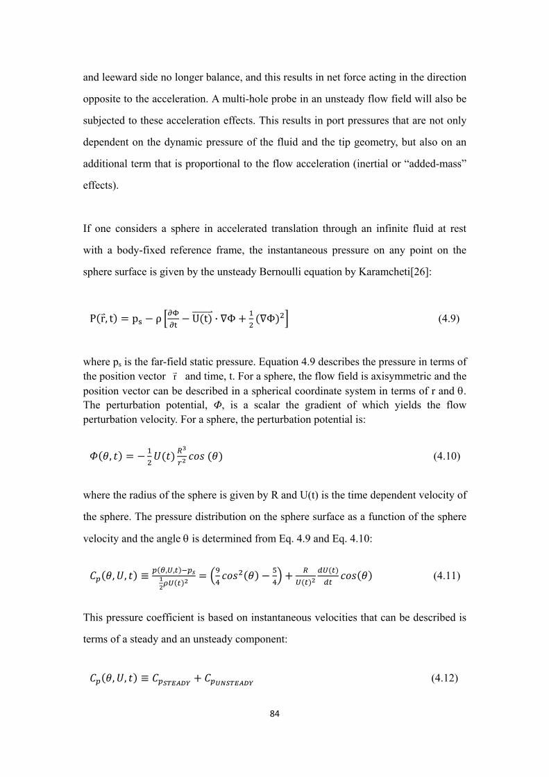
84  

and leeward side no longer balance, and this results in net force acting in the direction

opposite to the acceleration. A multi-hole probe in an unsteady flow field will also be

subjected to these acceleration effects. This results in port pressures that are not only

dependent on the dynamic pressure of the fluid and the tip geometry, but also on an

additional term that is proportional to the flow acceleration (inertial or “added-mass”

effects).

If one considers a sphere in accelerated translation through an infinite fluid at rest

with a body-fixed reference frame, the instantaneous pressure on any point on the

sphere surface is given by the unsteady Bernoulli equation by Karamcheti[26]:

P r, t p ρ U t · Φ Φ (4.9)

where ps is the far-field static pressure. Equation 4.9 describes the pressure in terms of the position vector rr and time, t. For a sphere, the flow field is axisymmetric and the position vector can be described in a spherical coordinate system in terms of r and θ. The perturbation potential, Φ, is a scalar the gradient of which yields the flow perturbation velocity. For a sphere, the perturbation potential is:

, (4.10)

where the radius of the sphere is given by R and U(t) is the time dependent velocity of

the sphere. The pressure distribution on the sphere surface as a function of the sphere

velocity and the angle θ is determined from Eq. 4.9 and Eq. 4.10:

, , , , (4.11)

This pressure coefficient is based on instantaneous velocities that can be described is

terms of a steady and an unsteady component:

, , (4.12)

85  

where:

(4.13)

(4.14)

This is the pressure distribution on the surface of the sphere, moving at velocity U(t),

in a fluid at rest. The same pressure distribution would also be seen if the sphere is

stationary and the flowfield is moving with velocity -U(t). For steady flows, the

inertial/unsteady term described by Eq. 4.14 vanishes and the pressure distribution on

the sphere surface is given by just the steady component. However, for accelerated

flows, the inertial term will be non-zero, and in the case of a multi-hole probe,

corrections must be made to accurately resolve the flow properties from the measured

port pressures. On the windward side of a sphere the viscous effects are small and the

pressure distribution is similar to the inviscid prediction.

In the previous analysis, the stagnation point was known and fixed, therefore only one

variable, the angle θ, was enough to describe the pressure anywhere on the sphere

surface. Now, however, as the flow angle with respect to the probe axis changes, the

stagnation point changes location as well. Thus, in order to describe the relative

position of the stagnation point with respect to a pressure port, two variables, the pitch

and yaw angles, α, β, are necessary. Also note that the pitch and yaw angles, α, β, are

global with respect to the probe axis and not local, with respect to the individual ports:

, , , , , , (4.15)

where i indicates the ith port of the multi-hole probe (for example, for a 5-hole probe, i

takes values from 1 to 5) . For general, non-periodic flows, the instantaneous

non-dimensional acceleration, K, is defined as:

(4.16)

86  

With this, and in order to express Cp as a function of K(t), we rewrite Eq. 4.15 as follows

, , , , (4.17)

where :

(4.18)

(4.19)

and for the sphere:

(4.20)

(4.21)

Note that the angle θ here is a function of α and β. For an actual probe, these

coefficients are determined by combining experimental approaches with the theory

described above. The non-dimensional acceleration, K, describes the magnitude of the

unsteady or inertial effects on the probe. From the equations it can be seen that the

error made by ignoring the inertial term, is linearly proportional to K, or equivalently,

linearly proportional to the probe size and the acceleration, and inversely proportional

to the square of the velocity. To demonstrate the point, consider a probe with a tip

diameter of 2 mm placed in an oscillating air stream at zero incidence. The flow

velocity is taken to be sinusoidal with a frequency of 2 kHz, a mean of 20 m/s and 10%

amplitude. The value of the non-dimensional acceleration coefficient is identical to

the error in magnitude if the inertial effects are ignored. For our example, the

calculated maximum K-value is 0.063, meaning that for the 2 mm probe in the

described flowfield, a maximum measurement error in the predicted dynamic pressure

of 6.3% is expected if the inertial effects are not accounted for. If the frequency is

increased to 20 kHz the maximum error in the predicted dynamic pressure will

increase to 63%.

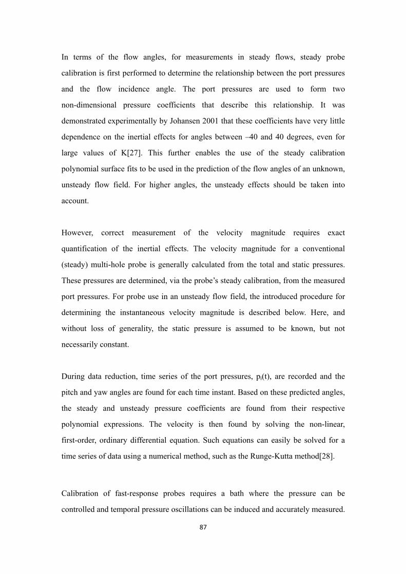
87  

In terms of the flow angles, for measurements in steady flows, steady probe

calibration is first performed to determine the relationship between the port pressures

and the flow incidence angle. The port pressures are used to form two

non-dimensional pressure coefficients that describe this relationship. It was

demonstrated experimentally by Johansen 2001 that these coefficients have very little

dependence on the inertial effects for angles between –40 and 40 degrees, even for

large values of K[27]. This further enables the use of the steady calibration

polynomial surface fits to be used in the prediction of the flow angles of an unknown,

unsteady flow field. For higher angles, the unsteady effects should be taken into

account.

However, correct measurement of the velocity magnitude requires exact

quantification of the inertial effects. The velocity magnitude for a conventional

(steady) multi-hole probe is generally calculated from the total and static pressures.

These pressures are determined, via the probe’s steady calibration, from the measured

port pressures. For probe use in an unsteady flow field, the introduced procedure for

determining the instantaneous velocity magnitude is described below. Here, and

without loss of generality, the static pressure is assumed to be known, but not

necessarily constant.

During data reduction, time series of the port pressures, pi(t), are recorded and the

pitch and yaw angles are found for each time instant. Based on these predicted angles,

the steady and unsteady pressure coefficients are found from their respective

polynomial expressions. The velocity is then found by solving the non-linear,

first-order, ordinary differential equation. Such equations can easily be solved for a

time series of data using a numerical method, such as the Runge-Kutta method[28].

Calibration of fast-response probes requires a bath where the pressure can be

controlled and temporal pressure oscillations can be induced and accurately measured.

88  

We constructed a chamber shown in Fig. 4.3, which is sealed and partially filled with

water. The space above the water surface communicates with a piston driven by an

electrical motor (Fig. 4.4). The frequency of the piston oscillation can be adjusted, and

thus a pressure fluctuation is transmitted to the water. Losses and inaccuracies of these

mechanical devices are not affecting the calibration process, because comparison of

pressure readings are made by a reference sensor placed next to the probe tip. The

reference pressure sensing element is placed inside the calibration chamber. The probe

tip is inserted in the same space, and direct comparison of the two readings is thus

made. The results show that for lower pressure fluctuation frequencies (less than

200Hz), the probe can response without attenuation (Fig. 4.5).

 

 

Fig. 4.3 Sketch of the dynamics calibration device of the fast‐response probe 

 

 

 

Fig. 4.4 Dynamics calibration mechanism for the fast‐response probe 

 

89  

 Fig. 4.5 Dynamcis calibration data 

 

4.3 Experiment layout

The five-hole probe system shown in Fig. 4.2 was used for flow field measurements in

three Dorr Oliver flotation cells with the same geometry but different sizes, but

extensive measurements covering all the sectors of the machine were only obtained in

the 6 m3 pilot cell (Fig. 4.6). The probe is mounted on a two-axes traversing system

which is controlled by a computer. The probe can also be translated along the third

axis manually (Fig.  4.7). Fig.  4.8 and Fig.  4.9  show the sketch of the rotor-stator

assembly as well as the coordinate system that we used. The Dorr-Oliver rotor has 6

blades while the stator has 16 blades. The origin of the coordinate system was set in

the middle of the rotor bottom. All the dimensions are normalized by rotor diameter

Di.

60 Hz

-500

0

500

1000

1500

2000

2500

3000

0 0.02 0.04 0.06

time (s)

pressure (Pa)

reference pressure

measured pressure

90  

 

 

Fig. 4.6 6m3 Dorr‐Oliver Pilot Cell

 

 Fig. 4.7 Layout of the test

 

91  

 

Fig. 4.8 Sketch of rotor‐stator assembly (side view)

 

 

Fig. 4.9 Sketck of rotor‐stator assembly (top view) 

 Fig. 4.10 Transformation of the coordinate system 

The five-hole probe returns components in the Cartesian coordinate system, i.e. Ux,

92  

Uy and Uz. Since the flotation tanks are cylindrical, we transfer the velocity

components to a cylindrical coordinate system for description convenience. As shown

in  Fig.  4.10, the probe is aligned with the x-axis facing the rotor. It is therefore

inclined by an angle θ with respect to the radial direction if it is displaced along the

y-axis.

(4.22)

The velocity components can be written in cylindrical coordinates as the follows:  

 sin                                                                                     (4.23) 

  (4.24)

(4.25)

Where, is the radial velocity, is the tangential velocity and is the

longitudinal velocity.

4.4 Results of turbulent flow measurement Turbulence intensity and Turbulent Kinetic Energy (TKE) of the single-phase

flow

The fast-response probe described above was placed at different locations of the 6m3

Dorr-Oliver pilot cell to map the turbulence characteristics. The probe was traversed

in the rotor-stator gap, where the highest turbulence level is expected. Turbulence

intensity, also often referred to as turbulence level, is defined as the root-mean-square

(RMS) of the turbulent velocity fluctuations normalized by rotor’s tip velocity. Fig. 

4.11 shows the turbulence intensity along a vertical line in the rotor-stator gap. As we

can see, the maximum turbulence level is 18% in the jet region. Such high turbulence

93  

levels are typical for inside rotating machinery. Turbulence levels of 20% were

reported in literature. Fig.  4.12 and Fig.  4.13 indicate the turbulent kinetic energy

(TKE), which is calculated based on turbulence intensity. We find that the turbulence

is very high in the jet region. We know that turbulence is rather low in the intake of

the impeller. This means that interaction with the edges of the blades both as the flow

enters the impeller region, and as it exits it is enough to generate turbulence before the

flow starts interacting with the stator plates.

 

Fig. 4.11 Turbulence intensity along a vertical line in rotor‐stator gap: Utip=6.4m/s, r/Di=0.57,  =11.25o

94  

 

Fig. 4.12 Normalized Turbulent Kinetic Energy (TKE) along a vertical line in rotor‐stator gap: Utip=6.4 m/s, r/Di=0.57,  =11.25o

 

Fig. 4.13 Turbulent Kinetic Energy (TKE) along a vertical line in rotor‐stator gap: Utip=6.4 m/s, r/Di=0.57,  =11.25o

The rotor tip velocity was varied (different Re number) to study its influence on the

turbulence level. From Fig.  4.14 we can see that the turbulence level has a slight

decrease with the reducing tip velocity in the jet region, while the absolute turbulent

kinetic energy (TKE) is proportional to the square of the rotor tip velocity (Fig. 4.14

and Fig. 4.15). These results indicate that at least for the range of the tip speeds tested,

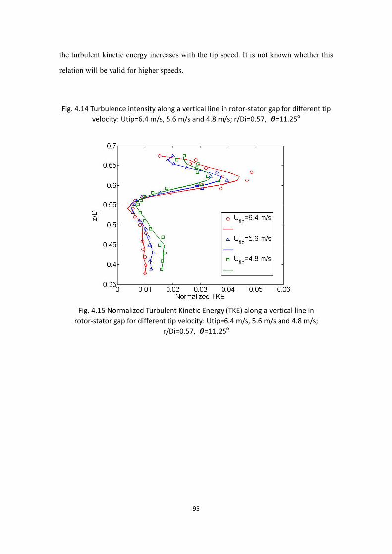
95  

the turbulent kinetic energy increases with the tip speed. It is not known whether this

relation will be valid for higher speeds.

 

Fig. 4.14 Turbulence intensity along a vertical line in rotor‐stator gap for different tip velocity: Utip=6.4 m/s, 5.6 m/s and 4.8 m/s; r/Di=0.57,  =11.25o

 

Fig. 4.15 Normalized Turbulent Kinetic Energy (TKE) along a vertical line in rotor‐stator gap for different tip velocity: Utip=6.4 m/s, 5.6 m/s and 4.8 m/s; 

r/Di=0.57,  =11.25o

96  

 

Fig. 4.16 Turbulent Kinetic Energy (TKE) along a vertical line in rotor‐stator gap for different tip velocity: Utip=6.4 m/s, 5.6 m/s and 4.8 m/s; r/Di=0.57,  =11.25o

Fig. 4.17 shows the turbulence intensity along vertical lines at different distances form

the center of the rotor. The line of r/.Di=0.57 corresponds to the line in the middle of

the rotor-stator gap, while the rest are the lines outside the stator which are 1”, 6” and

18” away from the edge of the stator. The flow’s turbulence intensity decreases

dramatically as we move out radially due to energy dispersion and dissipation. The

turbulence intensity in the rotor-stator gap is around 2.5 times of that in the far field

(18” away from the stator edge). The turbulence kinetic energy is shown in Fig. 4.18

and Fig. 4.19.

97  

 

Fig. 4.17 Turbulence intensity along vertical lines at different locations: Utip=6.4 m/s; =‐11.25 o, r/Di=0.57;  =‐2.9 o , r/Di =1.00, 1.26 and 1.88 

 Fig. 4.18 Normalized Turbulent Kinetic Energy (TKE) along vertical lines at different 

locations: Utip=6.4 m/s,  =‐2.9 o, r/Di=0.57, 1.00, 1.26 and 1.88 

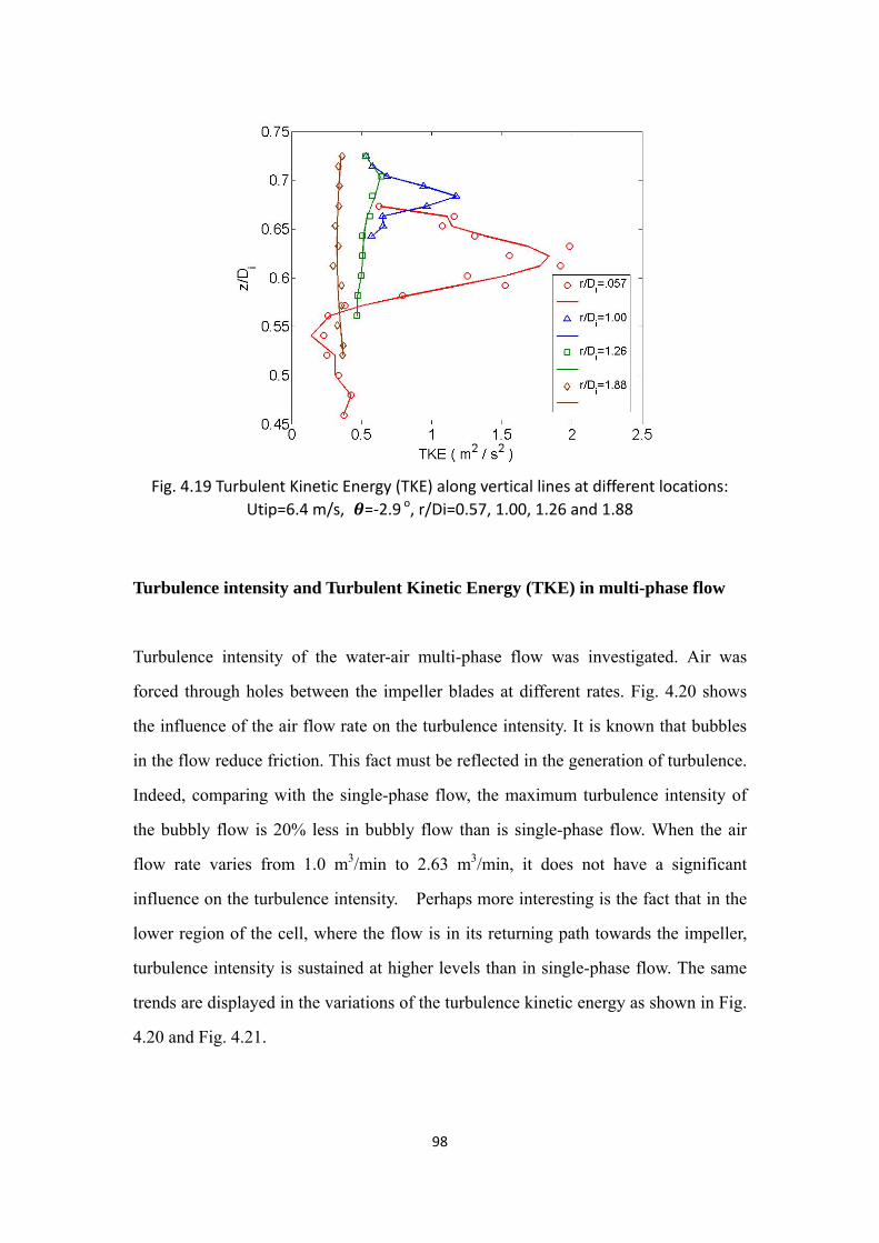
98  

 

Fig. 4.19 Turbulent Kinetic Energy (TKE) along vertical lines at different locations: Utip=6.4 m/s,  =‐2.9 o, r/Di=0.57, 1.00, 1.26 and 1.88 

Turbulence intensity and Turbulent Kinetic Energy (TKE) in multi-phase flow

Turbulence intensity of the water-air multi-phase flow was investigated. Air was

forced through holes between the impeller blades at different rates. Fig. 4.20 shows

the influence of the air flow rate on the turbulence intensity. It is known that bubbles

in the flow reduce friction. This fact must be reflected in the generation of turbulence.

Indeed, comparing with the single-phase flow, the maximum turbulence intensity of

the bubbly flow is 20% less in bubbly flow than is single-phase flow. When the air

flow rate varies from 1.0 m3/min to 2.63 m3/min, it does not have a significant

influence on the turbulence intensity. Perhaps more interesting is the fact that in the

lower region of the cell, where the flow is in its returning path towards the impeller,

turbulence intensity is sustained at higher levels than in single-phase flow. The same

trends are displayed in the variations of the turbulence kinetic energy as shown in Fig.

4.20 and Fig. 4.21.

99  

 Fig. 4.20 Turbulence intensity along a vertical line in rotor‐stator gap for different air flow rate: Qair=0, 1.0 m3/min, 2.0 m3/min and 2.63 m3/min; Utip=6.4 m/s; r/Di=0.57, 

=11.25o

 Fig. 4.21 Normalized Turbulent Kinetic Energy (TKE) along a vertical line in 

rotor‐stator gap for different air flow rate: Qair=0, 1.0 m3/min, 2.0 m3/min and 2.63 m3/min; Utip=6.4 m/s; r/Di=0.57,  =11.25o

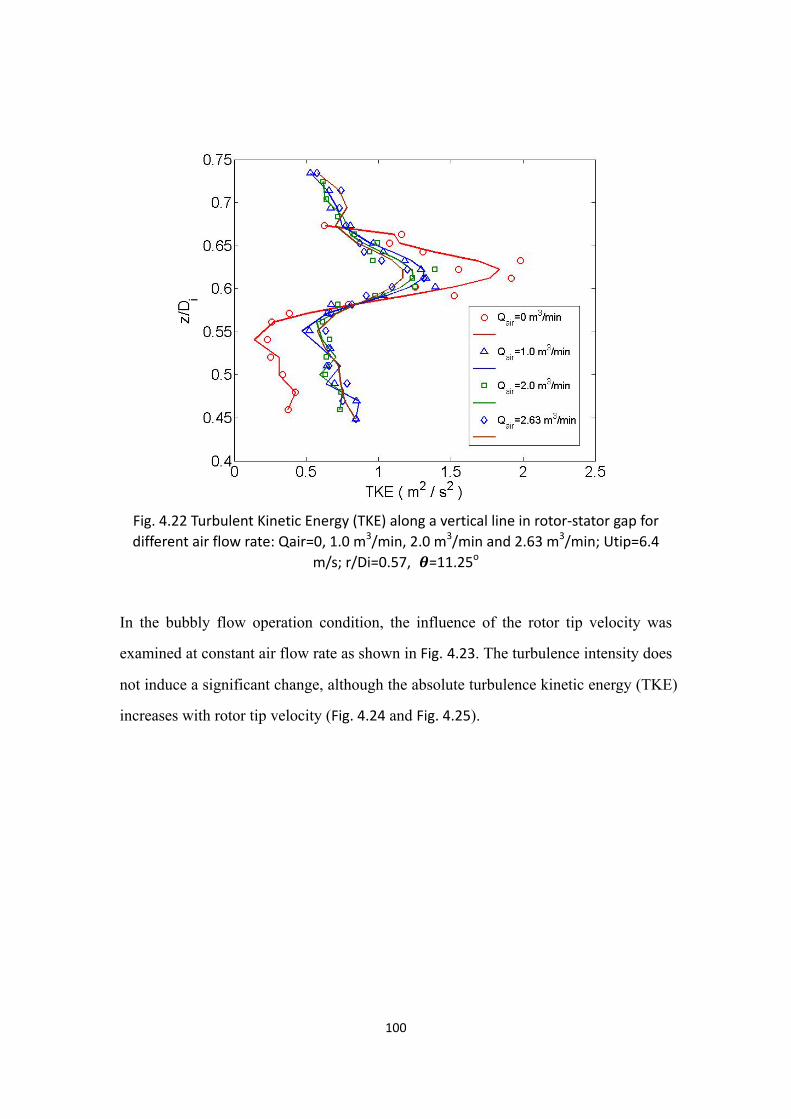
100  

 Fig. 4.22 Turbulent Kinetic Energy (TKE) along a vertical line in rotor‐stator gap for different air flow rate: Qair=0, 1.0 m3/min, 2.0 m3/min and 2.63 m3/min; Utip=6.4 

m/s; r/Di=0.57,  =11.25o

In the bubbly flow operation condition, the influence of the rotor tip velocity was

examined at constant air flow rate as shown in Fig. 4.23. The turbulence intensity does

not induce a significant change, although the absolute turbulence kinetic energy (TKE)

increases with rotor tip velocity (Fig. 4.24 and Fig. 4.25).

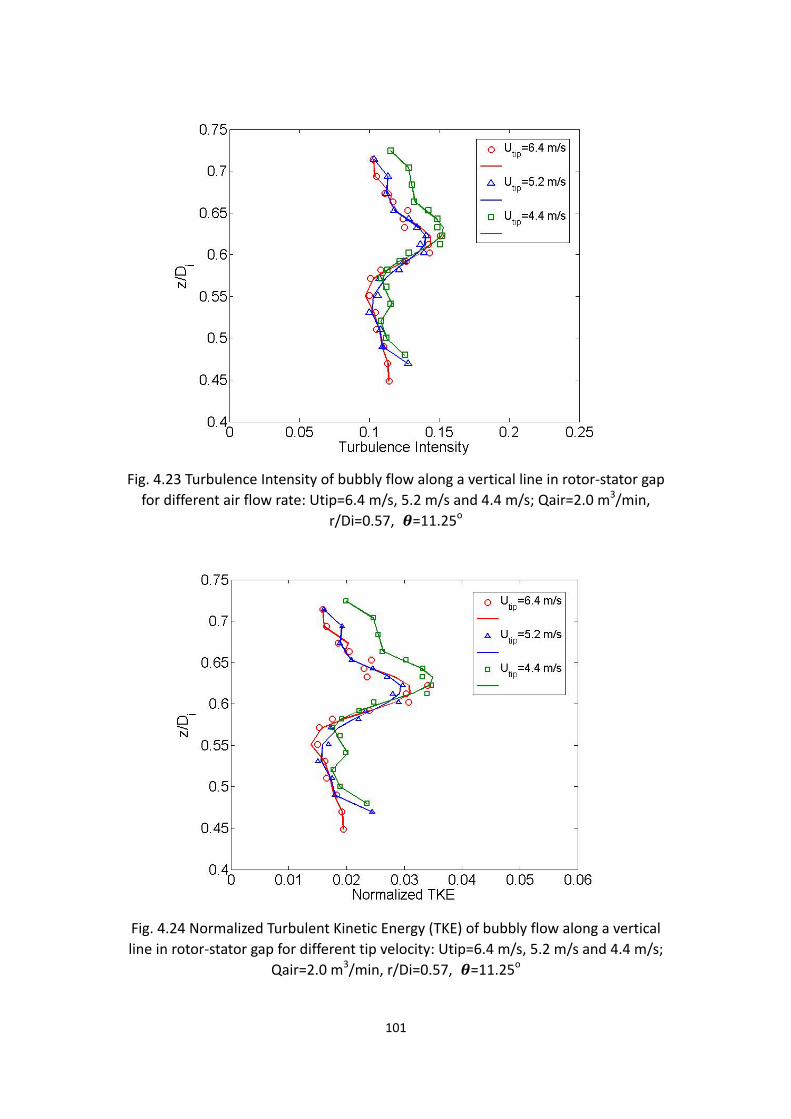
101  

 

Fig. 4.23 Turbulence Intensity of bubbly flow along a vertical line in rotor‐stator gap for different air flow rate: Utip=6.4 m/s, 5.2 m/s and 4.4 m/s; Qair=2.0 m3/min, 

r/Di=0.57,  =11.25o

 

Fig. 4.24 Normalized Turbulent Kinetic Energy (TKE) of bubbly flow along a vertical line in rotor‐stator gap for different tip velocity: Utip=6.4 m/s, 5.2 m/s and 4.4 m/s; 

Qair=2.0 m3/min, r/Di=0.57,  =11.25o

102  

 Fig. 4.25 Turbulent Kinetic Energy (TKE) of bubbly flow along a vertical line in 

rotor‐stator gap for different tip velocity: Utip=6.4 m/s, 5.2 m/s and 4.4 m/s; Qair=2.0 m3/min, r/Di=0.57,  =11.25o

Turbulence Dissipation Rate (TDR) in single-phase flow

As described in 4.1.2, the turbulence dissipation rates (TDR) are derived from the

turbulence kinetic energy. In Fig. 4.26 we see that the turbulence dissipation rate is

very high in the jet region. In Fig.  4.27 we see that the maximum turbulence

dissipation rate always appears at the same position, i.e. the jet region.

Fig.  4.28 shows the turbulence dissipation rate along vertical lines at different

distances from to the center of the rotor. The curve marked with r/.Di=0.57 presents

data obtained along a line in the middle of the rotor-stator gap, while the rest of the

curves present data obtained radially further out from the stator, at distances of 1”, 6”

and 18” away from the edge of the stator. As we can see, the flow’s dissipation rate

decreases sharply across the stator. This is followed by another significant decrease as

we move away from the stator, and then the decreases are somewhat moderated. In

103  

industrial systems, the maximum value of the local dissipation is up to 30 times

higher than its mean value. In this zone, the total power input dissipates and the

dispersion of air into bubbles and the bubble-particle interaction actively occur[29].

 Fig. 4.26 Turbulence Dissipation Rate (TDR) along a vertical line in rotor‐stator gap: 

Utip=6.4m/s, r/Di=0.57,  =11.25o 

 Fig. 4.27 Turbulence Dissipation Rate (TDR) along a vertical line in rotor‐stator gap for 

different tip velocity: Utip=6.4 m/s, 5.6 m/s and 4.8 m/s; r/Di=0.57,  =11.25o 

104  

 

Fig. 4.28 Turbulence Dissipation Rate (TDR) along a vertical lines at different locations: Utip=6.4 m/s,  =‐2.9 o, r/Di=0.57, 1.00, 1.26 and 1.88 

4.5 Summary and discussions

There are many advanced technologies and instruments for hydrodynamics

measurement, such as Particle Image Velocimetry (PIV) and Laser Doppler

Velocimetry (LDV). However these devices are only practical in well-controlled

laboratory environments, because they need very good optical access. Multi-hole

probes have been proved to be a robust, reliable and cost-efficient tool for stirring

tank turbulence measurement. We developed and tested new instrumentation that does

not require optical access. This cosnists of a fast-response five-hole water probe as

well as a calibration system

Turbulent flow properties in large-scale stirring tanks were measured successfully. An

empirical equation to calculate the turbulent dissipation rate in terms of large-scale

velocity fluctuations was examined and found to be reliable. We found that the

turbulence rates of the flow that enters the impeller are very low, but the rates increase

to their maximum values as the flow is discharged in the form of a jet in the upper

105  

part of the impeller. This implies that vorticity is generated mostly inside the impeller.

We also found that turbulence decreases continuously after it leaves the impeller

domain. This decrease is sharp at first and much milder later.

It was found that the introduction of air bubbles decreases the turbulence intensity of

the stream jet. But turbulence seems to be sustained in the tank as indicated by

measurements in the lower part of the cell. This may be significant, because it will

enhance bubble-particle collisions closer to the floor of the tank, where particles may

be falling and get agitated by turbulence.

106  

References 1. Schubert, H., On the turbulence controlled microprocesses in flotation

machines. International Journal of Mineral Processing 1999. 56: p. 257–276.

2. Liepe, F. and H. Möckel, Untersuchungen zum Stoffvereinigen in Flüssiger

Phase. Chemical Technology 1976. 28: p. (Jg., Heft 4).

3. Levins, B.E. and J.R. Glastonbury, Particle-liquid hydrodynamics and mass

transfer in a stirred vessel: Part 2 - Mass transfer. Transactions of the

Institution of Chemical Engineers, 1972. 50: p. 132-146.

4. Saffman, P.G. and J.S. Turner, On the collision of drops in turbulent clouds.

Journal of Fluid Mechanics, 1956. 1: p. 16-30.

5. Abrahamson, J., Collision rates of small particles in a vigorously turbulent

fluid. Chemical Engineering Science, 1975. 30: p. 1371-1379.

6. J.L.Lumley, H.T.a., A First Course In Turbulence. 1972, Cambridge,

Massachusetts: MIT Press.

7. Hinze, J.O., Turbulence. 1975, New York: McGraw-Hill, Inc.

8. Wu, H., Patterson, G.K., Laser-doppler measurements of turbulent-flow

parameters in a stirred mixer. Chemical Engineeering Science, 1989. 44(10): p.

2207-2221.

9. Lee, K.C., Yianneskis, M., Turbulence properties of the impeller stream of a

rushton turbine. AIChE Journal, 1998. 44(1): p. 13-24.

10. Baldi, M., Yianneskis, M., On the quantification of energy dissipation in the

impeller stream of a stirred vessel from fluctuating velocity gradient

measurements. Chemical Engineeering Science, 2004. 59: p. 2659-2671.

11. Gaskey, S., et al., A method for the study of turbulent mixing using

Fluorescence spectroscopy. Exper. In Fluids., 1990. 9: p. 137-147.

12. Law, A.W.K. and Wang H., Measurement of Mixing Processes With Combined

Digital Particle Image Velocimetry and Planar Laser Induced Fluorescence.

Experimental Thermal and Fluid Science, 2000. 22: p. 213-229.

13. Schafer, M., M. Hofken, and F. Durst, Detailed LDV Measurements For

107  

Visualization of The Flow Field Within A Stirred-Tank Reactor Equipped With

A Ruston Turbine. Trans IChemE, 1997. 75: p. 729-736.

14. Rao, M.A., Brodkey, R.S., Continuous Flow Stirred Tank Turbulence

Parameters in the Impeller Stream. Chem. Eng. Sci., , 1972. 27: p. 137-156.

15. Costes, J. and J.P. Couderc, Study by laser dopper anemometry of the

turbulenct flow induced by a rushton turbine in a stirred tank Chemical

Engineering Science, 1988. 43: p. 2751-2764.

16. Okamoto, Y., N. Nishikawa, and K. Hashimoto, Energy dissipation rate

distribution in mixing vessels and its effects on liquid-liquid dispersion and

solid-liquid mass transfer. International Chemical Engineering, 1981. 21: p.

88-94.

17. Piirto M., et al., Measuring Turbulence Energy with PIV in a Backward-facing

Step Flow. Experiments in Fluids, 2003. 35: p. 219-236.

18. Kresta, A.M. and P.E. Wood, The flow field produced by a pitched blade

turbine: characterization of the turbulence and estimation of the dissipation

rate. Chemical Engineering Science, 1993. 48: p. 1761-1774.

19. Senoo, Y., Y. Kita, and K. Ookuma, Measurement of Two-Dimensional

Periodic Flow With a Cobra Probe. Transactions of the ASME Journal of

Fluid Engineering, 1973. 2: p. 295-300.

20. Castorph, D. and J. Raabe. Measurement of Unsteady Pressure Unsteady

Relative velocity Field of a Kaplan Runner by Means of an Electronic

Multi-miniature Probe as a Basic Contribution to Research on Unsteady

Runner Load. in Proceedings of the 7th IAHR Symposium. 1974. Vienna.

21. Kerrebrock, J.L., W.T. Thompkins, and A.H. Epstein. A Miniature High

Frequency Sphere Probe. in ASME Symposium on Measurement Methods in

Rotating Components of Turbomachinery. 1980. New Orleans.

22. Koppel, P., et al., On The Development and Application of the Fast-Response

Aerodynamic Probe System in Turbomachines – Part 3: Comparison of

Averaging Methods Applied to Centrifugal Compressor Measurements.

108  

Journal of Turbomachinery, 2000. 122: p. 527-536.

23. Ng, W.F. and T.G. Popernack, Combination Probe for Hi-Frequency Unsteady

Aerodynamic Measurements. IEEE Transactions on Aerospace and Electronic

Systems, 1988. 24(1): p. 76-84.

24. Matsunaga, S., H. Ishibashi, and M. Nishi, Measurement of Instantaneous

Pressure and Velocity in Nonsteady Three-Dimensional Water Flow by Means

of a Combined Five-Hole Probe. Transaction of the ASME Journal of Fluid

Engineering, 1980. 102: p. 196-202.

25. Naughton, J.W., L.N. Cattafesta III, and G.S. Settles, Miniature Fast Response

Five-Hole Conical Probe for Supersonic Flowfield Measurements. AIAA

Journal, 1993. 31(3): p. 453-458.

26. Karamcheti, K., Principles of Ideal-Fluid Aerodynamics. 1966, New York:

John Wiley & Sons Inc.

27. Johansen, E.S., O.K. Rediniotis, and G.S. Jones, The Compressible

Calibration of Miniature Multi-Hole Probes. J. Fluids Eng., 2001. 123: p.

128-137.

28. Telionis, D.P., Y. Yang, and O.K. Rediniotis, Recent Developments in

Multi-Hole Probe (MHP) Technology, in 20th International Congress of

Mechanical Engineering. 2009: Gramado, Brazil.

29. Colloidal science of flotation, ed. A.V. Nguyen, Schulze, Hans Joachim. Vol.

118. 2004, New York: Marcel Dekker Inc.

 

109

Chapter 5 Dynamics of Bubble-particle Interaction

Single particle with varied contact angles were directed toward stationary air bubbles

in water, while monitoring the collision process by means of a high speed CCD

camera. The impact velocities and collision angles were controlled using an

electromagnetic gun. Away from the bubble surface, particle is subjected to weak

hydrodynamic and gravitational forces only. As the particle approached the bubble

surface within the diameter of the particle, the particle velocity is decelerated due to

the lubrication force. As the particle approached the bubble closer, the bubble-particle

interaction is controlled by surface forces (i.e., electrostatic, van der Waals and

hydrophobic forces). The particle-travel time and film-drainage times are measured. A

model is developed to predict these time scales, in which the bubble deformation was

taken into account.

5.1 Introduction

Flotation is the technology that separates valuable minerals from waste gangue using

air bubbles in a hydraulic environment where multiphase flow is involved. A typical

flotation cell is a cylindrical vessel with an agitator driving the fluid and generating

turbulence to enhance mixing. Selected mineral particles are hydrophobized by using

an appropriate reagent (collector). When the hydrophobized mineral particles collide

with air bubbles, they attach to air bubbles and rise to the free surface, while gangue

mineral particles remain in the pulp. Controlling the minerals’ hydrophobicity and

110

enhancing the bubble-particle collision and attachment rates are of critical importance

in flotation.

The capture of hydrophobic particles by air bubbles is a very complicated process

involving both hydrodynamic and surface forces. The bubble-particle interaction is

the fundamental process in flotation and many investigators have been working on

this problem for decades. However the principles that govern bubble-particle

collisions are far from full understood. Since this process is highly stochastic, it is

very hard to measure the collision in the cell directly. Several models have been

developed to predict the bubble-particle collision rate[1-3]. They can be simplified

into a general form.

(5.1)

where is the collision number, and are particle and bubble number

concentrations, respectively, and is the collision diameter, i.e., sum of particle and

bubble radii.

For simplicity, flotation kinetics is generally modeled as a first-order rate process,

involving various subprocesses such as collision, attachment, and detachment. The

attachment rate should be a function of the number concentrations of particles and

bubbles, while the detachment rate should be is related to the number concentrations

of bubble-particle aggregates.

111

1

12ZN

(5.2)

Where k is the flotation rate constant and P is probability of flotation. The

attachment and detachment probabilities depend on a wide range of complex factors,

for example, the hydrodynamic characteristics of the flotation cell and the sizes of

bubbles and particles. Yoon studied the effect of bubble size on fine particle

flotation[4].

Studies of single particles interacting with a bubble are useful to gain new

understanding of the flotation fundamentals. Efforts have been made by previous

researchers to study bubble-particle interaction. Bubble-particle interaction is divided

into three sub-processes: collision, attachment, and detachment. Collision is the

approach of a particle to encounter a bubble and is governed by the long-range

hydrodynamic forces. Once the particle approaches the bubble at a shorter separation

distance, surface forces begin to play a significant role and determine if the bubble-

particle attachment will occur or not. The bubble-particle aggregate can be detached

depending on the hydrodynamic forces relative to the forces holding the aggregates

together.

Flotation experiments with a single bubble were carried out to determinate the capture

efficiency of a bubble rising through a dilute mineral suspension[5, 6]. The capture

efficiency is defined as the fraction of the particles in the volume swept by a bubble

that is actually collected. Although it provides useful information, the technique is

still a stochastic process. To conduct direct observation of single bubble-particle

112

interaction, Guo used a capillary tube to generate a bubble with desired size in water

and then the bubble was released to impact with a bitumen drop held by a tube. The

entire bubble sliding and attachment process is recorded with high-speed camera. The

shortcoming of this method is that the collision velocity and angle are difficult to be

controlled[7]. Vella and Metcalfe studied the impact of a line mass onto a liquid-gas

interface by dropping a rod to the interface and found that the conditions on the mass

weight and impact speed affect whether it sinks or is trapped by the interface. The

results show that the collision is determined by Froude number and Weber number[8].

In this experiment, however, the mass enters liquid phase from gas phase, which is

opposite to what happens in flotation. Great efforts have been made to develop the

bubble-particle collision models. Dai reviewed various models for the calculation of

collision efficiencies between particles and bubbles[9]. These models do not take the

bubble deformation into account, however. Omota considered the deformation of the

bubble and developed a novel model describing the adhesion of particles to bubble,

but the experiments were conducted under a stagnant condition[10].

The objective of this work is to design a novel experiment to study the mechanism of

how a single particle immersed in a liquid collides with an air bubble. Particles were

shot toward stationary air bubble at controlled velocities and angles in hydraulic

environment, while monitoring the collision processes by a high speed camera. The

images are analyzed to calculate the particle travel time and film drainage time. A

model has been developed to predict the collision process, including the effect of

bubble deformation.

113

5.2 Experiments

5.2.1 Experimental setup

To study the bubble-particle interaction, a novel apparatus was designed and built.

This instrument is inspired by coil-gun, or more professionally, electromagnetic pulse

accelerator. As the name implies, the major part of a coil-gun is a coil of wire. Once a

large current is pulsed through the coil, a strong magnetic field is created, with the

electromagnetic force pulling a ferromagnetic object through the center of the coil as

shown in Fig. 5.1. The terminal velocity of the projectile depends on many

parameters, for example, the current intensity, the number of coil loops, the length of

the coil tube and the mass of the projectile. Power is supplied to the electromagnet

coil from some sort of a fast discharge storage device, typically a bank of high-

capacity high voltage capacitors designed for fast energy discharge. A diode is

installed to protect polarity sensitive capacitors from damage due to inverse polarity.

The circuit diagram of the power supply is shown in Fig. 5.2. The capacitors need to

be pre-charged to a certain voltages. Once the solid-state switch is turned on, a

currency pulse will form in the coil to generate strong magnetic field. Ideally, 100%

of the magnetic flux generated by the coil will be delivered to and act on the

ferromagnetic projectile, but this is often far from the case due to the air-core-

solenoid/projectile construction as well as heat loss. However, the initial velocities of

the projectiles increase monotonously with the charging voltage.

114

Fig. 5.1 Sketch of coil gun 

Fig. 5.2 Circuit diagram of bubble‐particle collision device 

Fig. 5.3 Bubble‐particle collision device 

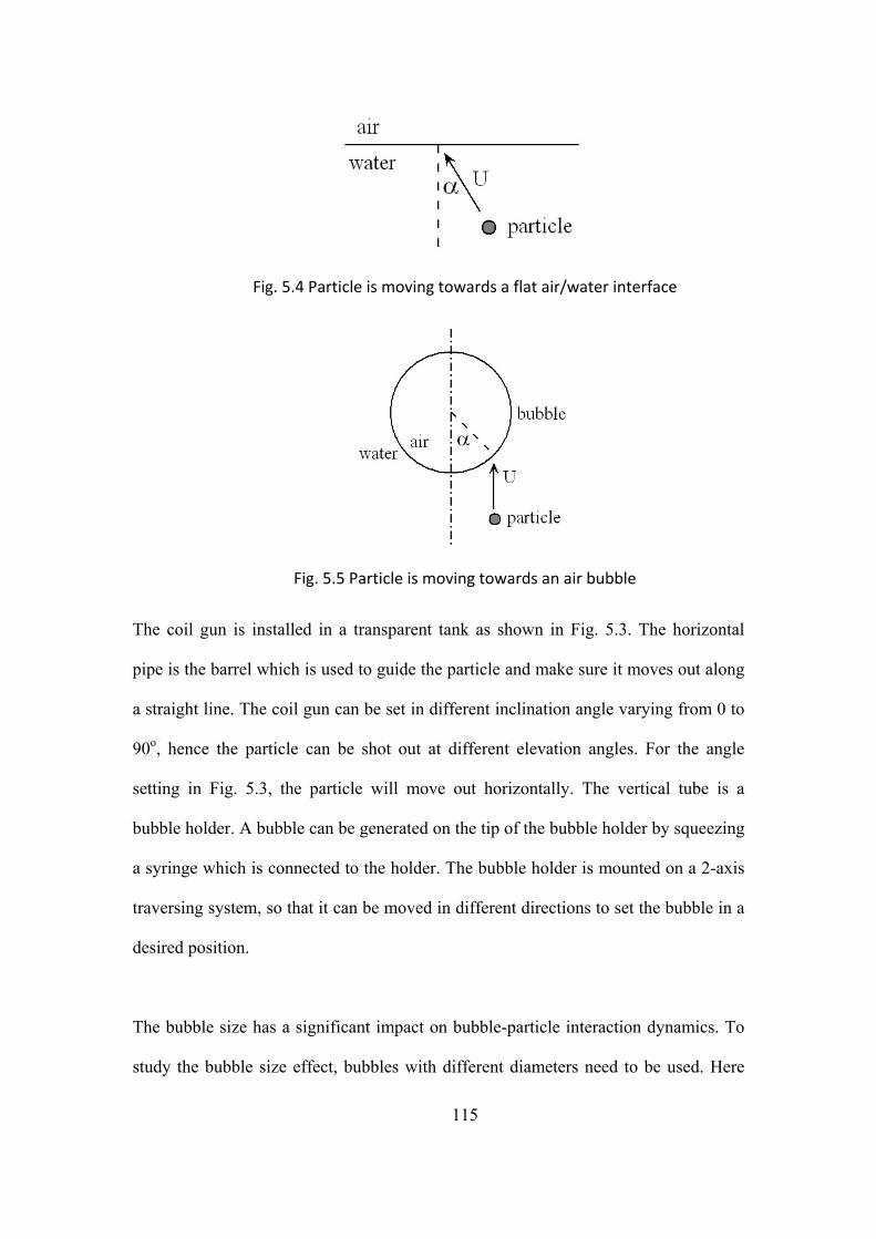
115

Fig. 5.4 Particle is moving towards a flat air/water interface 

Fig. 5.5 Particle is moving towards an air bubble 

The coil gun is installed in a transparent tank as shown in Fig. 5.3. The horizontal

pipe is the barrel which is used to guide the particle and make sure it moves out along

a straight line. The coil gun can be set in different inclination angle varying from 0 to

90o, hence the particle can be shot out at different elevation angles. For the angle

setting in Fig. 5.3, the particle will move out horizontally. The vertical tube is a

bubble holder. A bubble can be generated on the tip of the bubble holder by squeezing

a syringe which is connected to the holder. The bubble holder is mounted on a 2-axis

traversing system, so that it can be moved in different directions to set the bubble in a

desired position.

The bubble size has a significant impact on bubble-particle interaction dynamics. To

study the bubble size effect, bubbles with different diameters need to be used. Here

116

two extreme cases are examined for comparison. As shown in Fig. 5.4, the particle is

shot towards a free interface, which can be considered a portion of an infinity bubble.

Fig. 5.5 shows that a particle is shot towards a small bubble with a diameter of a few

millimeters. Both the impact velocity and angle can be controlled. The particles used

here is 0.4 mm diameter stainless steel spheres. The surface of the particles was

treated chemically to adjust their contact angle. Here, the contact angle of particles

varies from 0 to 90 o. In this communication, the results obtained at contact angle of

90o are presented and discussed.

5.2.2 Experimental observation

Particle Impinging on a Flat Bubble Surface

Fig. 5.6 shows the images of a particle (θ = 90o) shot toward a flat air/water interface,

which may be regarded part of an infinitely large bubble, from underneath. For

analytical convenience, time zero is set when the particle reaches the highest point. As

the particle impinges on the interface, the air/water interface deforms as shown in Fig.

5.7. Due to the changes in curvature, the pressure of the liquid in the thin film formed

between the particle and bubble becomes higher than the liquid pressure in the far

field, which will lead to film drainage. At this point, the driving force for the film

drainage is the capillary pressure (ΔP) associated with the changes in curvature. When

the film becomes thinner within the range of approximately 200 nm, however, the

film thinning process will also be controlled by the disjoining pressure (Π) created by

the surface forces.

117

To describe the process of bubble-particle interaction, two different time scales are

defined here. One is the particle-travel time, Ttrav, which is the time span for the

particle in contact with the air/liquid interface. As shown in Fig. 5.6, the first frame,

the apex of the particle reaches the flat air/water interface before it deforms at t = -

2.25 ms, and reaches the highest elevation at t = 0 s when particle velocity becomes

zero. The time scale from the first to the fourth frame is defined as the travel time.

The other time scale is the film-drainage time, Tdrain, representing the time it takes for

the two interfaces (solid/liquid and air/liquid) to coalesce, which is similar to the

concept of induction time. The particle-travel time can be measured by analyzing the

video clips. Intuitively, two interfaces coalesce or the thin film ruptures only if the

film-drainage time is shorter than the particle-travel time, i.e. Tdrain≤Ttrav. For the

case of a particle with contact angle of 90o as shown in Fig. 5.6, we found that Ttrav =

2.25 ms. Tdrain is about the same. Methods of determining the latter will be described

in another communication.

Fig. 5.6 Particle impinges with flat interface (impact velocity: 0.564 m/s) 

118

Fig. 5.7 Particle impacts with flat interface: dimple configurations 

Fig. 5.8 Particle impinges with air bubble (impact velocity: 0.554 m/s) 

Particle Impinging on a air bubble

Fig. 5.8 shows the results obtained for the interaction between a spherical steel

particle of 0.4 mm diameter with θ = 90o and a spherical bubble of 2.4 mm diameter.

One can see that Ttrav is ~1.25 ms. Since the particle attaches to the bubble as shown

in Fig. 5.8, we can say that Tdrain < Ttrav. We found that is less than 1.125 ms

in anther experiment. It may be interesting to note here that for the spherical

bubble (Fig. 5.8) is considerably shorter than the case with the flat bubble (Fig. 5.6),

119

which can be attributed to the curvature difference. In general, smaller bubbles should

create higher capillary pressures according to the Young-Laplace equation.

5.3 Theoretical model

We consider the multiphase system that a particle immersed in a liquid moves toward

an air bubble. Such dynamics is coupled with various forces from gravity, drag,

surface tension, and disjoining force. When the particle approaches an air/liquid

interface, a thin liquid film forms, which begins to thin initially due to surface tension

force. When the film thickness reaches the range where negative disjoining pressure

becomes significant, the film becomes unstable and ruptures.

Using the lubrication approximation, which is applicable at film thicknesses much

smaller than particle size, we can derive an equation of motion by considering the

force balance as follows,

(5.3)

Here, ρ and ρs are densities of fluid and particle, R the particle radius, g the

gravitational constant, μthe fluid viscosity, δ the fluid gap thickness between the

particle and air, γ the surface tension coefficient, φ the angle of interface, and h and ζ

are the particle and the air/liquid interface position from the equilibrium interface,

respectively. The term on the left-hand side corresponds to the acceleration force of

ρs −ρ2

⎛ ⎝ ⎜

⎞ ⎠ ⎟

4π3

R3 d2hdt 2 = −(ρs − ρ)g

4π3

R3 + 6πμr2

δdhdt

+ 2γRd sinφ

120

the particle with the added mass, and the terms on the right-hand side are the

gravitational (buoyant) force, the lubrication drag, and the surface tension from the

top interface. Details of geometry and parameters are further illustrated in Fig. 5.9.

Fig. 5.9 Schematics of the air‐liquid‐particle system 

Simply, this hydrodynamic problem of a particle colliding into the air/liquid interface

can be characterized by five non-dimensional numbers. The Weber number is a ratio

of fluid inertia to surface tension, defined as We = ρU2R/γ. The Froude number is a

ratio of inertia to gravitational force, defined as Fr = U/(gR)1/2. The Reynolds number

is a ratio of inertia to viscous forces, defined as Re = ρUR/μ. In addition, the ratio of a

fluid thickness and the particle size is Δ = R/δ and the ratio of particle to fluid

densities is D=ρs/ρ. By introducing non-dimensional parameters as h=RH, t=(R/U)τ

in addition to these numbers, the basic governing equation becomes

ϕπττ

sin31Re9111

211 22

2

DWeddH

DFrDdHd

D−

Δ−⎟

⎠⎞

⎜⎝⎛ −−=⎟

⎠⎞

⎜⎝⎛ − (5.4)

121

Typically, our experiments have been conducted in U ~ 0.5 m/s with the steel particle

(R~0.2 mm). Corresponding non-dimensional numbers are We~1, Fr ~ 10, Re ~ 100,

D ~10, Δ ~ 200. Then, the above equation further simplifies to

ϕπττ

sin31Re91

22

2

DWeddH

DFrdHd

−Δ

−−= (5.5)

Here, sin φ nonlinearly depends on H and other parameters. In order to solve

the equation or express it in terms of a single variable, sin φ needs to be evaluated in

two extreme cases; small and large slopes of the air/liquid interface.

For the small slope (φ<<1 or ), the angle is estimated as sinφ ~ (1-H)R/lc

by using the Young-Laplace equation and .Then, the

above basic equation is rewritten as only a function of H as

013113Re9

22

2

=⎟⎟⎠

⎞⎜⎜⎝

⎛++−

Δ+

DWelR

FrH

DWelR

ddH

DdHd

cc ππττ (5.6)

Now, the equation is solvable in a form of a linear homogeneous second order

ODE, the same as describing a dashpot system with damped oscillations. However,

this small slope approximation is not valid in most cases of our experiments with high

particle velocities.

dζ /dr <<1

d2ζ /dr2 + dζ /rdr

1+ (dζ /dr)2( )3 / 2 =ζlc

2 R = h + ζ

122

When the slope is very high (φ~π/2), sinφ can be approximated as a constant. Hence,

the above equation is simplified as

0311Re9

22

2

=⎟⎟⎠

⎞⎜⎜⎝

⎛++

Δ+

πττ DWeFrddH

DdHd (5.7)

The solution for the particle position becomes

1)1)/(exp( 2113 −−−−= ττ CCCCH (5.8)

where the three constants are,.

( ) )1(,)/(3/1,)9/()(Re 21132

21 CCCCWeDFrCDC +−=+=Δ= π

By expanding this solution, H in terms of non-dimensional time τ, the above

expression reduces to

)(1211 32

21

0 τττ OCC

UH +⎟⎟⎠

⎞⎜⎜⎝

⎛+++−= (5.9)

Finally, the characteristic time scale of the particle motion is estimated from the

constant in the τ2- term

2/1

2

311Re9

−

⎟⎟⎠

⎞⎜⎜⎝

⎛++

Δ=

πDWeFrDURTtrav (5.10)

This time approximately represents the time duration for the test particle to stay in the

interface. Specifically, this represents the time interval between the time when a

particle is located close to the air/liquid interface and the time when it moves away

123

from the interface. For convenience, we denote the above characteristic time as “the

particle-travel time” which is determined by combined effects of gravity, surface

tension, and inertia. For the case of a spgerical particle of 0.4 mm approaching a flat

air/water interface, Ttrave is about 2 milliseconds which is in a good agreement with

our experimental observation.

Coalescence process occurs only if a particle stays at the interface sufficiently longer

than the time for draining the liquid film in between. This film-drainage time

corresponds to the time for the film to thin down to a critical thickness δc. Beyond this

critical thickness, the film becomes unstable and spontaneously ruptures. In the next

few paragraphs, we will discuss on the film-drainage time.

When the particle approaches an air/liquid interface with a high velocity, the thin fluid

layer is compressed and the pressure in the film becomes higher than pressure in the

far-field (bulk). As the film drains due to the radial pressure gradient, and eventually

ruptures at δc. At high impact velocities, the radial pressure gradient in a thin film can

be estimated using the Bernoulli equation as

Π−≈−=R

PPu bulkfilmRγρ 2

2 (5.11)

where uR is the mean radial velocity in the thin liguid film, and Π is the

disjoining pressure. From the continuity equation, the thinning rate of the film

thickness δ is written in terms of radial velocity as

124

2/1

)(2⎟⎟⎠

⎞⎜⎜⎝

⎛⎟⎠⎞

⎜⎝⎛ Π−−=−= δγ

ρδδδ

RRu

Rdtd

R (5.12)

Here, the film thinning rate is given as a function of disjoining pressure which

has a strong dependence on the film thickness due to the presence of surface forces

such as the van der Waals force, electrostatic force, hydrophobic force, and possibly

more. The study of expressing the disjoining pressure in terms of the film thickness

by itself is worth publishing a separate article. For simplicity in this bubble-particle

dynamics, we assume that the disjoining pressure is constant at Π0 and is independent

of film thickness. Then, the solution of the film thickness δ is obtained as

⎟⎟

⎠

⎞

⎜⎜

⎝

⎛⎟⎟⎠

⎞⎜⎜⎝

⎛⎟⎟⎠

⎞⎜⎜⎝

⎛ Π−−= t

RU

UWet

2/1

20

012exp)(

ρδδ (5.13)

As mentioned above, the film-drainage time is defined as the time interval when the

film thickness reaches the critical film thickness δc from the initial thickness δ0. Then,

the film-drainage time for the thin film to rupture becomes

⎟⎟⎠

⎞⎜⎜⎝

⎛⎟⎟⎠

⎞⎜⎜⎝

⎛⎟⎟⎠

⎞⎜⎜⎝

⎛ Π−

−

cdrain UWeU

RTδδ

ρ0

2/1

20 ln12

21~ (5.14)

By using physical parameters used in our experiments and assuming δ0~R/5, δc~50

nm, the film-drainage time calculated from this equation is about 1.5 milliseconds,

which is also close to the values from our experimental observations.

125

After the time Tdrain, the thin fluid film is no longer stable enough to keep the air

bubble separate from the approaching particle.

In summary, we have evaluated two time scales analytically. The first one is the

particle-travel time, Ttrav, which is the time span for the particle resting on the

air/liquid interface. Secondly, the film-drainage time, Tdrain, is the duration for two

interfaces (solid/liquid and air/liquid) to coalesce by draining the fluid film in

between. Estimated times using physical parameters are in good agreement with

experimental measurement.

Intuitively, two interfaces coalesce or the thin film ruptures only if the particle-travel

time is longer than the film-drainage time. This condition, i.e., Ttrav > Tdrain, concludes

the inequality as.

2

02

02 ln12311

Re9

−

⎟⎟⎠

⎞⎜⎜⎝

⎛⎟⎟⎠

⎞⎜⎜⎝

⎛⎟⎟⎠

⎞⎜⎜⎝

⎛ Π−<⎟

⎟⎠

⎞⎜⎜⎝

⎛++

Δ

cUWeDWeFrD δδ

ρπ (5.15)

Coalescence only occurs as long as the inequality holds. This inequality is more

probable when the magnitude on the left-hand side becomes smaller. In other words,

the tendency for the coalescence increases in the cases of large Re, Fr and We as

observed in the present work.

126

5.4 Conclusions and discussions

In this paper, we have studied the dynamics of particle impinging onto air bubbles or

flat air/water interfaces. From experiment, the bubble-particle dynamics is observed to

exhibit two different interactions; the particle either is attached to the air/liquid

interface or bounces back. This transition can be characterized by two times scales,

involving the particle-travel and film-drainage times. For example, a hydrophobic

particle coalesces with an air bubble when the particle-travel time is longer than the

film-drainage time. Our model predicts these time scales are close to a few

milliseconds, which agrees well with experimental observations. In addition, we

observed that larger bubble has longer drainage time than smaller bubble, which can

be explained by the curvature difference. Large bubble deforms due to low pressure in

the air phase, which increases the length scale of the thin liquid film (TLF). This in

turn increases the drainage time as the liquid must flow through a longer length of

TLF. A small bubble can resist to deformation better due to high capillary pressure,

which in turn helps keep the length scale of TLF small and hence the decrease the

drainage time. Therefore, smaller bubbles are more effective for bubble-particle

attachment owing to the shorter drainage times.

127

References

1. Abrahamson, J., Collision rates of small particles in a vigorously turbulent

fluid. Chemical Engineering Science, 1975. 30: p. 1371-1379.

2. Kruis, F.E. and K.A. Kusters, The collision rate of particles in turbulent flow.

Chemical Engineering Communications, 1997. 158: p. 201-230.

3. Pyke, B., D. Fornasiero, and J. Ralston, Bubble particle heterocoagulation

under turbulent conditions. Journal of Colloid and Interface Science, 2003.

265(1): p. 141-151.

4. Yoon, R.H. and G.H. Luttrell, The effect of bubble size on fine particle

flotation. Mineral Processing and Extractive Metallurgy Review, 1989. 5: p.

101-122.

5. Dai, Z., et al., The inertial hydrodynamic interaction of particles and rising

bubbles with mobile surfaces. J. Colloid Interface Sci., 1998. 197: p. 275-292.

6. Sarrot V., et al., Experimental Determination of Particles Capture Efficiency

in Flotation. Chemical Engineering Science, 2007. 62: p. 7359-7369.

7. Gu, G., et al., A Novel Experimental Technique to Study Single Bubble-

Bitumen Attachment in Flotation. Int. J. Miner. Process, 2004. 69: p. 235-250.

8. Vella, D. and P.D. Metcalfe, Surface tension dominated impact. Physics of

Fluids, 2007. 19: p. 072108.

9. Dai, Z., D. Fornasiero, and J. Ralston, Particle-bubble collision models: a

review. . Advances in Colloid and Interface Science, 2000. 85: p. 231 - 256.

10. Omota, F., A.C. Dimian, and A. Bliek, Adhesion of solid particles to a gas

bubble. Part 1: modelling. Chemical Engineering Science, 2006. 61: p. 823-

834.

128  

Chapter 6 Summary and Outlook

6.1 Summary

 

In this dissertation, efforts were made to investigate a few fundamental

hydrodynamics problems of the flow in stirring tanks. Most of the work was

conducted in flotation cells. Flotation cells are industrial pieces of equipment for

solid/solid separation. The flotation process involves bubble and particle

hydrodynamics, bubble-bubble, particle-particle and bubble-particle interactions,

which is a great challenge for theoretical analysis, experimental detection and

numerical simulation. Since the flotation process occurs in a multi-phase flow

environment, hydrodynamic characteristics have significant impact on the machine’s

performance.

Flotation machines need to be designed to maximize bubble-particle collisions. The

performance of flotation cells is influenced by physical features and operating

conditions. The efficiency depends critically on multi-phase flow hydrodynamics. To

understand the flotation process, optimize machine design and enhance efficiency, the

following efforts were undertaken.

1. A 5-hole probe was built and employed in Dorr-Oliver flotation cells to obtain flow

pattern measurements. The results indicate that the flow in the Dorr-Oliver flotation

cell is driven by a jet issuing out from the very top of the rotor. There is a substantial

circumferential component in this jet. The flow is then redirected by stator blades and

emerges out from the stator in almost the radial direction. The 16-stator blades divide

the cell volume into 16 sectors, each of which has a similar flow pattern due to the

symmetry. The windward side region of each stator plate is receiving a strong jet, and

therefore it is immersed in an energetic flow region. The flow on the leeward side has

very slow motion and is not involved in the flotation process as actively as the

windward side. After emerging from the stator, the jet deflects in anticipation of its

encounter with the tank side walls, and forms two toroidal regions, which are isolated

from each other. Mixing between these regions is due only to the turbulent shearing

interface between them. As a result, the top region is almost quiescent, while the

129  

bottom is violently agitated. Additionally, the mass exchange between the two regions

is very weak. That means there may not be enough solid particles entering the

quiescent zone to collide with bubbles and thus participate in the flotation process.

But bubble-particle aggregates penetrate the interface between the two regions and

rise to form froth.

2. Once the bubbles are generated, they are dispersed into the bulk by the stream. The

air dispersion has direct influence on bubble-particle collision. Designers need to

make sure that bubbles and particles populate the same domains in a machine.

Otherwise no collisions would occur. To study how the air bubbles are distributed, a

novel isokinetic sampling probe system was developed. This system can be used to

take true samples in a tank. The samples are analyzed automatically to generate local

void fraction information. The measurement results show that the air is dispersed

almost uniformly into the whole tank, even in the dead zone.

3. Once bubbles and particles appear in the same location, energy is needed to

increase the collision frequency. Bubbles and particles obtain energy from turbulence.

It is very difficult to measure the motion of individual bubbles and particles,

especially in industrial facilities. However, the slip velocities of bubbles and particles

can be calculated using empirical models. To conduct the turbulence measurement, a

fast-response five-hole probe was designed, fabricated and calibrated. Measurements

show that the flow near the rotor has very high turbulence levels (up to 18%). As the

stream moves out radially, the turbulence level decreases to 7%. The turbulence

dissipation rate in the rotor-stator gap is about 20 times higher than that near the tank

wall, which means that most of the energy is dissipated in the rotor-stator region.

4. Since the slip velocity can be calculated based on turbulence dissipation rate, an

experiment was set up to simulate the bubble-particle collision with controlled impact

velocity and angle. As the separation distance between bubble and particle is less than

the diameter of the particle, the particle is decelerated due to the lubrication force. As

the distance is further reduced, the bubble-particle interaction is controlled by surface

forces (i.e., electrostatic, van der Waals and hydrophobic forces). The experimental

results show that there are four modes for the impact process: attach, attach-detach,

bounce back and penetrate, all controlled by the impact energy. The criterion is that if

the fluid drainage time is less than the residence time, attachment will occur,

130  

otherwise, the particle will bounce back. Measurements show that the residence time

is on the order of milliseconds, which is also predicted by our model.

6.2 Outlook: bubble-particle aggregates detection in flotation tanks

Once a flotation machine is designed and optimized based on the research results, a

validation is needed to test its performance. We can just run the real flotation and

measure the final recovery rate as a black box. A more attractive informative method

is to explore the processes that take place inside it. A device is needed to monitor the

flotation process under water. To answer such questions, photographic samples are

needed to be taken at different locations underwater. A new isokinetic borescope

system was developed for this purpose. This new system has been tested in lab cell

and some preliminary results are shown in this section. In the future, it can be applied

to pilot cells and even commercial cells.

 

An isokinetic boroscope system was developed to take photographic samples in-situ.

This probe was tested and applied to detect the bubble-particle aggregates in flotation

cells.

Development of isokinetic borescope system

 

The design of isokinetic borescope system is based on the isokinetic probe described

in 3.2.1. The difference is that the isokinetic sampling probe has a transparent window

in the middle. The system (Fig.  6.1) includes a rigid boroscope, a camera and fiber

optics to deliver light. When the system was submerged in the flow, the isokinetic

probe was aligned with the flow, and isokinetic conditions were established by

adjusting the probe’s pump’s speed. The rigid boroscope attached to the isokinetic

probe window was used to take photos without submerging the camera. The miniature

tip makes it convenient to map the entire tank point by point.

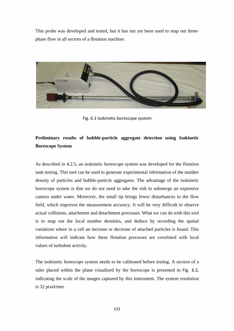
131  

This probe was developed and tested, but it has not yet been used to map out three-

phase flow in all sectors of a flotation machine.

 

Fig. 6.1 Isokinetic borescope system 

 

Preliminary results of bubble-particle aggregate detection using Isokinetic

Borescope System

 

As described in 4.2.5, an isokinetic borescope system was developed for the flotation

tank testing. This tool can be used to generate experimental information of the number

density of particles and bubble-particle aggregates. The advantage of the isokinetic

borescope system is that we do not need to take the risk to submerge an expensive

camera under water. Moreover, the small tip brings fewer disturbances to the flow

field, which improves the measurement accuracy. It will be very difficult to observe

actual collisions, attachment and detachment processes. What we can do with this tool

is to map out the local number densities, and deduce by recording the spatial

variations where in a cell an increase or decrease of attached particles is found. This

information will indicate how these flotation processes are correlated with local

values of turbulent activity.

The isokinetic borescope system needs to be calibrated before testing. A section of a

ruler placed within the plane visualized by the borescope is presented in Fig.  6.2,

indicating the scale of the images captured by this instrument. The system resolution

is 32 pixel/mm.

132  

 

Fig. 6.2 Calibration Image of the isokinetic borescope system 

The isokinetic borescope system was tested in the 10” diameter Dorr-Oliver bench

machine. The experiment settings are described as the follows:

Tank diameter: 254 mm

Rotor diameter: 70 mm

Particle material: solid glass sphere

Particle size: 203 microns, monosize

Solid concentration: 0.5%

Surfactant: 2 ppm

Collector: 3g/tone

Air superficial velocity: 0.4 cm/s

The detection tip of the system was inserted in the jet region close to the stator. The

probe direction and suction rate were adjusted to achieve the isokinetic suction

condition before photos were taken.

133  

 

Fig. 6. 3 Bubble‐particle aggregates detection 

Fig. 6. 3 shows that the isokinetic borescope can record bubbles, particles and bubble-

particle aggragates. It should be emphasized that this image captured bubbles and

particles that are moving at high speed. The monosize circles are particles as pointed

out by red arrow. The bubble size varies from 0.53 mm to 1.66 mm. At present, we

can just identify bubble-particle aggragates manually. Though challenging, the

computer image processing of such images is feasible in the future. A color camera

and dyed particles will make the identification easier.

134  

 

 

Fig. 6.4 Particles attach to different size bubbles 

 

Fig. 6.5 Particles attach to each other 

 

From Fig. 6. 3, Fig. 6.4 and Fig. 6.5, we can see that particles can attach to bubbles with different size, and the particles also attach to each other forming clusters.