Revised Version - Experimental and Numerical study of a conical helically coiled, single phase heat...
20
1 Experimental and Numerical study of a Conical Helically Coiled, Single Phase Heat Exchanger Daniel Flórez-Orrego a,1 , Walter Arias b , Héctor Velásquez b . a Polytechnic School, University of São Paulo, Av. Prof. Mello Moraes, 2231, São Paulo, Brazil. b Minas Faculty, National University of Colombia, Carrera 80 #65-223, Medellín, Colombia, [email protected], [email protected] Abstract: Complex fluid dynamic and heat transfer process present in curved tube heat exchangers confer them some advantages over the straight tubes in terms of area to volume ratio and enhancement of heat and mass transfer coefficients. In this work, an analysis of the single phase heat transfer process in a conical helically coiled heat exchanger non-previously studied was carried out. An empirical correlation for the determination of average Nusselt number along the duct, with Reynolds number ranging between 4300 and 18600 has been developed. Also, numerical simulations were performed using ANSYS FLUENT® 12.1 software, for simultaneously solving the equations of mass, momentum and heat transport, using realizable κ-ε two equations turbulence model. Cross section velocity contours and vector components were compared with those of conventional helical tubes configurations (non-conical). It was found there are similarities in terms of the main flow skewness, but there are slight differences on the trajectories of core fluid particles in the secondary flow. Also, pressure drop calculated using Ito and White’s correlations were compared with numerical and experimental data, concluding that experimental data lies between those results predicted by the other authors’ correlations. Finally, numerical and experimental Nusselt number has been compared with the ones obtained using the correlations proposed by Seban and McLaughlin and by Xin and Ebadian for curved tubes. It was found that those correlations overestimate the values obtained for the conical helically coiled heat exchanger, whereas experimental and a numerical results presented a good agreement. Keywords: Single phase, Conical helically coiled, Heat exchanger, Nusselt Correlation, Friction factor coefficient. 1. Introduction Complex fluid dynamics occurring in curved tubes have been an invariant issue of research for last few decades [1]. The operating principle of the curved tubes and the benefits attributed to them over the performance of the straight tubes can be summarized as follows: (a) generation of secondary flow in the radial direction; (b) enhanced cross-sectional mixing; (c) reduction in axial dispersion and (d) improved heat transfer coefficient [1]. Other advantages of helical tubes are their high ratio of heat transfer area to occupied volume, their good adaptability to cylindrical shapes and an excellent performance in the presence of thermal expansion, behaving as a spring. Secondary flow is a consequence of the difference in axial momentum between fluid particles in the core and the wall regions. The core fluid experiences a centrifugal force that pushes it to the outer wall of the coil, from where is redirected towards the inner wall in two different streams throughout the upper and lower walls of the tube, as it is shown in Fig. 1. 1 Corresponding author. Tel.: +55-11-974982315; E-mail address: [email protected] (D. Flórez-Orrego).
Transcript of Revised Version - Experimental and Numerical study of a conical helically coiled, single phase heat...

1
Experimental and Numerical study of a Conical Helically Coiled, Single Phase Heat Exchanger
Daniel Flórez-Orregoa,1
, Walter Ariasb, Héctor Velásquez
b.
a Polytechnic School, University of São Paulo, Av. Prof. Mello Moraes, 2231, São Paulo, Brazil. b Minas Faculty, National University of Colombia, Carrera 80 #65-223, Medellín, Colombia,
[email protected], [email protected]
Abstract:
Complex fluid dynamic and heat transfer process present in curved tube heat exchangers confer them some advantages over the straight tubes in terms of area to volume ratio and enhancement of heat and mass transfer coefficients. In this work, an analysis of the single phase heat transfer process in a conical helically coiled heat exchanger non-previously studied was carried out. An empirical correlation for the determination of average Nusselt number along the duct, with Reynolds number ranging between 4300 and 18600 has
been developed. Also, numerical simulations were performed using ANSYS FLUENT® 12.1 software, for
simultaneously solving the equations of mass, momentum and heat transport, using realizable κ-ε two equations turbulence model. Cross section velocity contours and vector components were compared with those of conventional helical tubes configurations (non-conical). It was found there are similarities in terms of the main flow skewness, but there are slight differences on the trajectories of core fluid particles in the secondary flow. Also, pressure drop calculated using Ito and White’s correlations were compared with numerical and experimental data, concluding that experimental data lies between those results predicted by the other authors’ correlations. Finally, numerical and experimental Nusselt number has been compared with the ones obtained using the correlations proposed by Seban and McLaughlin and by Xin and Ebadian for curved tubes. It was found that those correlations overestimate the values obtained for the conical helically coiled heat exchanger, whereas experimental and a numerical results presented a good agreement.
Keywords:
Single phase, Conical helically coiled, Heat exchanger, Nusselt Correlation, Friction factor coefficient.
1. Introduction
Complex fluid dynamics occurring in curved tubes have been an invariant issue of research for last
few decades [1]. The operating principle of the curved tubes and the benefits attributed to them over
the performance of the straight tubes can be summarized as follows: (a) generation of secondary
flow in the radial direction; (b) enhanced cross-sectional mixing; (c) reduction in axial dispersion
and (d) improved heat transfer coefficient [1]. Other advantages of helical tubes are their high ratio
of heat transfer area to occupied volume, their good adaptability to cylindrical shapes and an
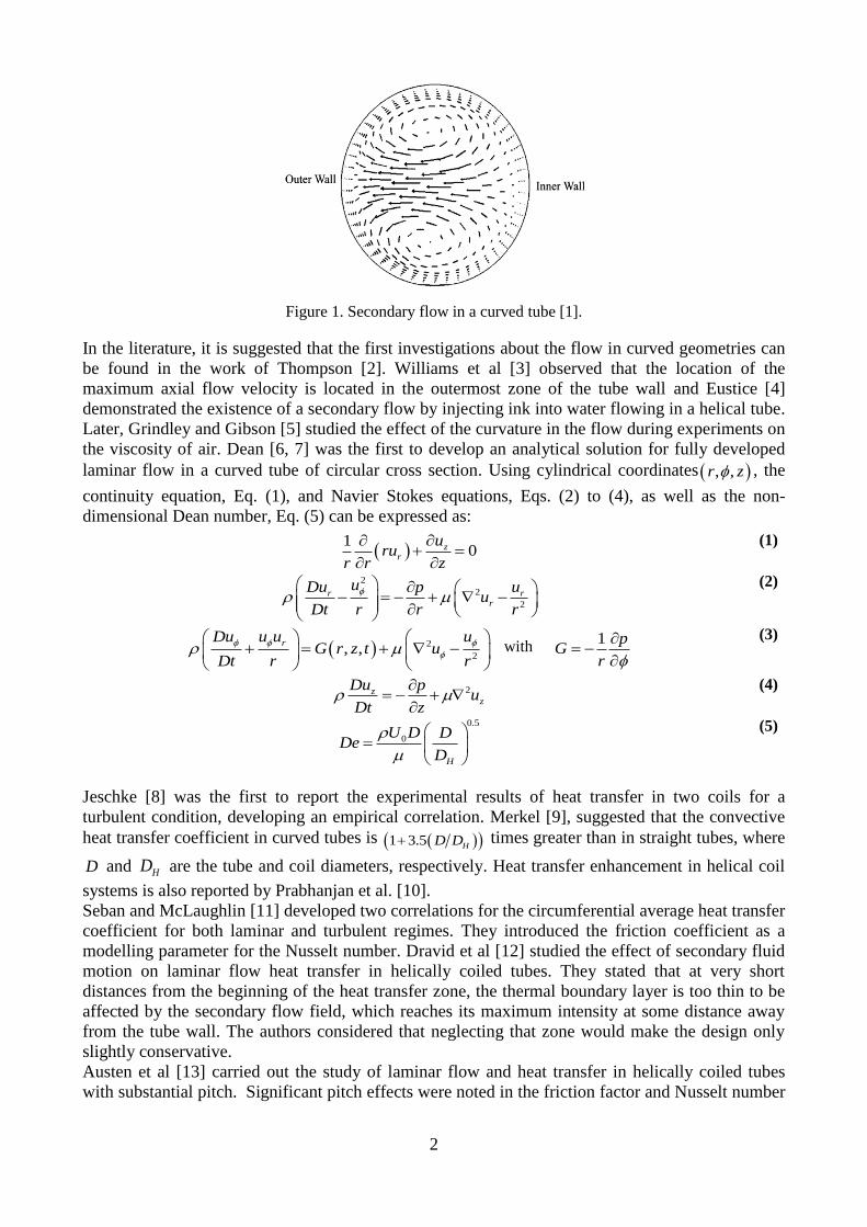
excellent performance in the presence of thermal expansion, behaving as a spring. Secondary flow
is a consequence of the difference in axial momentum between fluid particles in the core and the
wall regions. The core fluid experiences a centrifugal force that pushes it to the outer wall of the
coil, from where is redirected towards the inner wall in two different streams throughout the upper
and lower walls of the tube, as it is shown in Fig. 1.
1 Corresponding author. Tel.: +55-11-974982315;
E-mail address: [email protected] (D. Flórez-Orrego).
2
Figure 1. Secondary flow in a curved tube [1].
In the literature, it is suggested that the first investigations about the flow in curved geometries can
be found in the work of Thompson [2]. Williams et al [3] observed that the location of the
maximum axial flow velocity is located in the outermost zone of the tube wall and Eustice [4]
demonstrated the existence of a secondary flow by injecting ink into water flowing in a helical tube.
Later, Grindley and Gibson [5] studied the effect of the curvature in the flow during experiments on
the viscosity of air. Dean [6, 7] was the first to develop an analytical solution for fully developed
laminar flow in a curved tube of circular cross section. Using cylindrical coordinates , ,r z , the
continuity equation, Eq. (1), and Navier Stokes equations, Eqs. (2) to (4), as well as the non-
dimensional Dean number, Eq. (5) can be expressed as:
1
0zr
uru
r r z
(1)
2
2
2
r rr
uDu upu
Dt r r r
(2)
2
2, ,
rDu u u uG r z t u
Dt r r
with 1 p
Gr
(3)
2zz
Du pu
Dt z
(4)
0.5
0
H
U D DDe
D
(5)
Jeschke [8] was the first to report the experimental results of heat transfer in two coils for a
turbulent condition, developing an empirical correlation. Merkel [9], suggested that the convective
heat transfer coefficient in curved tubes is 1 3.5 HD D times greater than in straight tubes, where
D and HD are the tube and coil diameters, respectively. Heat transfer enhancement in helical coil
systems is also reported by Prabhanjan et al. [10].
Seban and McLaughlin [11] developed two correlations for the circumferential average heat transfer
coefficient for both laminar and turbulent regimes. They introduced the friction coefficient as a
modelling parameter for the Nusselt number. Dravid et al [12] studied the effect of secondary fluid
motion on laminar flow heat transfer in helically coiled tubes. They stated that at very short
distances from the beginning of the heat transfer zone, the thermal boundary layer is too thin to be
affected by the secondary flow field, which reaches its maximum intensity at some distance away
from the tube wall. The authors considered that neglecting that zone would make the design only
slightly conservative.
Austen et al [13] carried out the study of laminar flow and heat transfer in helically coiled tubes
with substantial pitch. Significant pitch effects were noted in the friction factor and Nusselt number

3
at low Reynolds numbers. These effects were attributed to free convection, and they diminished as
Reynolds number increased.
Xin and Ebadian [14] presented an experimental assessment on heat transfer in helical tubes. The
authors explored two values of curvature for Re ranging from 5000 to 1.105, and Prandtl ranging
from 0.7 to 175. They proposed the following correlation 0.92 0.40.00619Re Pr 1 3.455 HNu D D .
Cioncolini et al [15] studied the curvature effects on the laminar to turbulent flow transition from
direct inspection of experimental Nusselt number profiles. Due to the coil curvature, the process of
turbulence emergence in the tested coils was found to be much more gradual and smooth than it was
in straight tubes, enhancing the effect as the coil curvature increases. By inducing the secondary
flow, the coil curvature increases both the hydraulic resistance and the heat transfer effectiveness,
with respect to straight tube flow.
Jayakumar et al [16] carried out experimental and CFD studies in a fluid-to-fluid heat exchanger in
order to compare the transport phenomena inside a helical coil for various boundary conditions.
They also compared the effect of using constant and temperature-dependent fluid properties in the
computational modelling of heat transfer. Standard κ-ε turbulence model was implemented. A
correlation in the form 0.9112 0.40.025 PrNu De was proposed.
Conte et al [17] performed numerical simulations to understand forced heat transfer in laminar fluid
flow using rectangular coiled tubes with circular cross-section and characterized by curvature and
torsion parameters. The focus was addressed on exploring the flow pattern and temperature
distribution through the tube. Later, Conte et al [18] compared the outside convective heat transfer
coefficient for conical and conventional helical coils. The results showed a better heat transfer
performance for the conical coil case, since an effective flow arrangement triggers a more intense
turbulence. No investigations were carried out for the inner convective heat transfer coefficient.
Kumar et al [19] modelled the fluid flow and heat transfer process in a tube-in-tube helically coiled
heat exchanger for different fluid flow rates. The renormalization group (RNG) k–ε model is used
to model the turbulent flow in the heat exchanger. New empirical correlations were developed for
hydrodynamic and heat-transfer processes in the outer tube.
Di Piazza et al [20] presented a systematic attempt to assess the applicability of alternative
turbulence models for the prediction of pressure drop and heat transfer in coiled tubes. They
concluded that the SST eddy viscosity/eddy diffusivity model and the second order Reynolds
stress model give comparable results for the friction factor f correlated by Ito [21] and the
Nusselt number correlated by Pethukov’s momentum-heat transfer analogy [20].
Various correlations for the pressure drop friction factor, f, were proposed by Ito [21], White [22]
[23], Hart et al [24] and Mishra and Gupta [25]. The former is the most popular correlation.
An extensive review about the flow and heat transfer characteristics is provided by Naphon and
Wongwises [26]. The latest review was published by Vashisth et al [1].
Currently, the various types of curved tube geometries are classified as follows: (a) torus (constant
curvature and zero pitch), (b) helically coiled tube (constant curvature and pitch), (c) serpentine
tubes (periodic curved tubes with zero pitch) with bends or elbows, (d) spirals (Archimedean
spirals), and (d) twisted tubes. Other different curved chaotic configurations have been developed as
a course of technological development [27] [28]. At the author’s knowledge, only a work with a
conical helically coiled heat exchanger has been published, and the analysis was focused on the heat
transfer in the outer side of the tube [18].
At this work, both experimental and numerical investigations were performed for the purpose of
investigating the heat transfer in a conical helically coiled heat exchanger. The simulation method is
concerned with laminar and turbulent flow of an incompressible fluid (water) using commercial
computational fluid dynamics (CFD) software ANSYS® Fluent 12.1; the velocity profiles are
compared with those reported for non-conical coiled heat exchangers (Fig. 1). Experimental average
Nusselt number and pressure drop friction factors f are compared with those predicted using

4
correlations proposed by other authors. Finally, a Nusselt number correlation for the conical
helically coiled heat exchanger used in this study is proposed.
2. Characteristics of the conical helically coil heat exchanger
2.1. Geometrical characteristics
Figure 2 shows the characteristics of the conical helical coil. The tube has an inner diameter of
D=7.904 mm and wall thickness of e=0.813 mm. The conical coil has major base and minor base
diameters of DMH = 150 mm and DmH = 75 mm, respectively (measured between the centers of the
tube). Meanwhile, the distance between two adjacent turns, called pitch, is the sum of inner
diameter D plus twice wall thickness. The mean coil diameter is defined as the average between
DMH and DmH, namely DH = 112.5 mm. The ratio of coil diameter to tube diameter (DH/D) is called
curvature ratio, and is equal to λ = 14.23. Coil length (L) and tube length (LP) are 400 mm and
12000 mm, respectively.
Figure 2. Coil geometry parameters (units in millimetres).
2.2. Critical Reynolds number
Similar to Reynolds number (Re) in straight tubes flow, another parameter used to characterize the
flow in a helical tube is Dean number, De, which was defined as Re HDe D D . The curvature of
the coil governs the centrifugal force while the pitch influences the torsion to which the fluid is
subjected to. The centrifugal force results in the development of a secondary flow. Many
researchers have found that transition from laminar to turbulent flow is delayed because of the
presence of secondary flow [1]. They have correlated the critical Reynolds number (or the Reynolds
number for which laminar to turbulent flow transition take place) as a function of curvature ratio.
Ito [21] derived a correlation to calculate the critical Reynolds number at which transition occurs,
given by Eq. (6): 0.6Re 2000 1 13.2c
(6)
valid in the range of 5 2000 . Srinivasan et al [29] proposed the following correlation for the
critical Reynolds number in curved tubes, Eq. (7):
0.5Re 2100 1 12c (7)
valid in the range of 7.5 100 . Cioncolini et al [30] have found that, for low values of the
curvature ratio (λ<24), an no abrupt transition from laminar to turbulent flow was observed. In
those cases, the friction factor decreased monotonically with Reynolds number, and the transition to

5
turbulence is indicated only by a change in the slope of the f - Re curve, occurring at a Reynolds
number which the authors approximated by the correlation: 0.47Re 30000c
(8)
with 7 24 .
3. Experimental set up
3.1. Experimental facility
The material used to construct the conical helically coiled heat exchanger is copper tubing. Winding
is manually performed using a special wood matrix for accomplishing the desired major and minor
diameters of the coil. Distortion of the cross section is minimized used sand filling. The conical
helically coil is provided with straight entry and exit hydrodynamic lengths. An entry length, about
21 tube diameters, is used as a hydrodynamic developing length, while the exit length is about 40
tube diameters. Both extensions are tangentially attached to the coil, which lies horizontally.
The test section of the coil is enclosed in a heat insulated AISI 430 stainless steel jacket, covered
with stone wool. The power heat supply is provided by burning liquefied petroleum gas (LPG) and
controlled by regulating the pressure at the burner inlet. Combustion gases are led through the inner
chamber of the coil and left it through a chimney. It is assumed that the flame uniformly irradiate
the surface of the coil, although condensed vapour water and sooting on its surface are also
observed. This fact can slightly alters constant wall heat flux assumption, but it is still reasonable to
assume a linear increase in the bulk temperature along the whole length, which is checked with
thermocouples attached to the outer wall of the tube (See Fig. 3).
The cold fluid enters the tube from the connection at the minor diameter of the coil and the hot fluid
leaves the tube through the connection at the major diameter of the coil, and finally it is discharged
into a water reservoir. A counter-flow heat transfer process between water and combustion product
gases is achieved (Fig. 3). A needle valve regulates the flow rate while it is measured by a
calibrated rotameter at the fluid inlet section. Pressure and temperature of the cold and hot fluids are
measured using a bourdon manometer and an immersion K-type thermocouple whose values are
available on digital displays. Before the test, the thermocouples are calibrated in situ at the water
supply temperature. Tube wall temperatures are monitored by six contact K-type thermocouples
separated each 6.7cm along the coil height. The details of the facility are given in Fig. 3.
Figure 3. Scheme of the experimental facility.

6
3.2. Experimental procedure
The tests are conducted using cold water coming from the local water supply service at 295K. For
each test, cold water flow rate and heat supply are fixed and before any data is recorded, the system
is allowed to approach the steady state. Then, the cold water flow rate is increased keeping the same
heat supply and repeating the experiment. After that, heat supply is increased and new increments
of the cold water flow rate are carried out, so that different heat transfer rates, pressure drop
conditions and flow regimes are created. The temperature and pressure at the inlet and outlet fluids,
as well as the temperature at each position in the outer wall of the tube are recorded six times and
averaged in the period of time. Besides of the rotameter, the mass flow rates are also determined by
collecting the flow into a graduated vessel (600 ml) while recording the time, as an alternative way
of measurement. All the thermodynamic and transport properties of water are calculated using the
SteamTab™ software, developed by the Chemicalogic Corporation for the thermodynamic and
transport properties of water and steam [31]. In the present experimental work the heat transfer
coefficient and heat transfer rates are calculated based on the measured pressure, temperature and
flow rate. The heat transferred to the cold water flowing inside the conical helically coiled heat
exchanger is calculated from Eq. (9):
2 1 2 1Q m i m i i i i
(9)
where is calculated as an average of the outlet and inlet densities of the fluid, being a function of
pressure and temperature. The heat transfer coefficients are calculated using Eq. (10):
avg
Qh
A T
where
,2 ,2 ,1 ,1
2
w b w b
avg
T T T TT
(10)
and where w, b, 2, and 1 stands for wall, bulk, outlet and inlet, respectively. Average heat transfer
coefficients are computed in a non-dimensional form given by Nusselt number, Eq. (11):
f w f avg
hD Q DNu
k A k T
(11)
where wA and fk are the internal heat transfer area of the tube and the fluid conductivity,
respectively. The later one is calculated as an average of the inlet and outlet fluid conductivities.
The Reynolds and Prandtl numbers are defined in the conventional way as shown in Eq. (12) and
(13):
4Re
f
m
D
(12)
Prp f
f
c
k
(13)
Where f and pc are the fluid dynamic viscosity and heat capacity calculated as an average of the
inlet and outlet fluid properties.
By varying the wall heat flux and mass flow rate, a total of 25 experiments are carried out. Heat
supply ranges between 5000 and 17000 W and volumetric flow rate varies between 2.50x10⁻⁵
and
8.17x10⁻⁵
m3/s, or equivalently 1.5 and 4.9 l/min. Reynolds number ranges between 4300 and
18600, whereas Prandtl number ranges between 2 < Pr < 6.
The following simplifications are assumed: 1) Steady state flow, 2) Fully hydrodynamic and
thermal developed flow; 3) Uniform wall heat flux; 4) Axial conduction in the tube wall and fluid is
neglected and 5) Peripheral temperature is uniform [32] [12]. The later assumption is valid if it is
considered the thickness and thermal conductivity of the tube. Peripheral differences diminishes
even more with high mass flow rates [13].

7
The difference between the inner and outer wall temperatures of the tube can be calculated
assuming one-dimensional (radial) heat conduction throughout the tube thickness, a uniform
volumetric rate of heat generation in the tube and an insulated boundary condition at the outer wall
[13]. Solving the appropriate conduction equation with those boundary conditions, it can be easily
shown that the temperature difference across the wall at any axial location is given by Eq. (14):
2 2 2
, , 2 ln4
ow o w i o o i
w i
rqT T r r r
k r
(14)
Where the uniform rate of heat generation can be calculated as 2 2
T o iq Q L r r .
4. Numerical Set up
A CFD methodology has been used to investigate the performance of the conical helically coiled
heat exchanger. In this research work, a commercial CFD package ANSYS® Fluent v12.1 (double
precision, 3D version) and a computer with Intel® Core™ i5-2430M Processor (3M Cache, 2.40
GHz) with 4GB RAM are used; each run has taken 12 hours.
4.1. Computational grid
The simulation geometry is created using SOLIDWORKS® 2009 mechanical design software and
then exported to ANSYS Fluent as Parasolid geometry modelling format. The meshing is achieved
using the ANSYS Fluent Meshing module. In this model, the tube wall thickness is not considered
and only the fluid control volume is modelled. A structured grid with 5 inflation layers is used to
refine the mesh near the surface of the control volume. On the other hand, an unstructured mesh is
used in the interior volume cells. The grid for the analysis domain is shown in Fig. 4.
This grid is composed of 3.499.443 nodes and 3.312.000 elements. The maximum skewness
reported is 0.4852 and the minimum is 0.01121. This implies good-to-excellent cell quality. The
grid given in Fig. 4 is chosen because a further refinement does not result in a reduction of mass and
energy residual errors.
Fig. 4. Grid used in the analysis of the fluid flow and heat transfer process.
4.2. Boundary conditions and CFD modelling
Four representative heat transfer and flow conditions are numerically analysed (Table 1). The
steady state, pressure-based type solver with an absolute velocity formulation is used. In both
laminar and turbulent cases, energy, momentum, and turbulence model (if applicable) equations are
solved. The environmental operating conditions are defined as 295K and 0 Pascal absolute
operating pressure.

8
For thermal equation, constant wall heat flux boundary condition is stated at the interface between
the wall and the fluid (See Fig. 5). For momentum equation, the wall is treated as a non-slip,
adiabatic and smooth wall. In all the cases, the cold fluid inlet temperature is kept as constant at
295K and the analyses are carried out varying the flow rate. At the fluid inlet, velocity inlet
boundary condition is specified. For the hot fluid outlet, pressure outlet boundary condition at zero
back pressure is specified. The acceleration of gravity is considered as 9.8m/s2, oriented to –X
coordinate direction (Fig. 5).
Fig. 5. Specified boundary conditions.
For the coil used in this study, the critical Reynolds number at which the transition from laminar to
turbulent flow regime occurs is calculated using Ito’s correlation [21] and it is equal to Re 7679c .
According to this, only the fourth condition shown in Table 1 represents a laminar flow regime and,
in this case, the laminar model in ANSYS Fluent simulation is considered.
For the turbulent regimes simulations, the Realizable turbulence model with Standard Wall
function is used. An immediate benefit of the realizable model is that it is likely to provide
superior performance for flows involving rotation, boundary layers under strong adverse pressure
gradients, separation, and recirculation. Initial studies have shown that the Realizable model
provides the best performance of all the model versions for several validations of separated
flows and complex secondary flow features [33]. Model constants are defined as: 1 1.44C ,
2 1.9C , 1.0 , 1.2 [33]. For fully-developed turbulent internal flow, the Intensity I and
Hydraulic Diameter D are specified. The turbulence intensity at the core of a fully-developed flow
is estimated from the Eq. (15), derived from an empirical correlation in circular ducts [34]:
18
'0.16 Re
uI
u
(15)
Turbulence intensity of 1% or less is considered as low and turbulence intensity greater than 10% is
considered as high. Turbulent Kinetic energy and turbulent dissipation rate are calculated
using the Eq. (16) and (17) [34]:
23
2avgu I
(16)
3 23 4C
(17)
Where avgu is the mean velocity inlet, is the length scale (= 0.07D) and C is an empirical
constant specified in the turbulence model, approximately 0.09. The turbulence length scale, , is a
physical quantity related to the size of the largest eddies that contain the energy in turbulent flows.
In fully-developed flows in ducts, it is restricted by the size of the duct, since the turbulent eddies
cannot be larger than the duct. The factor of 0.07 is based on the maximum value of the mixing
length in fully-developed turbulent tube flows [35]. In all the turbulent cases a turbulent length scale

9
of 0.0005533m and a hydraulic diameter of 0.007904m are considered. Turbulence Intensity,
Turbulent kinetic energy and Turbulent dissipation rate are shown in Table 1.
Table 1. Boundary and Cell zone conditions.
Condition
Volumetric
flow rate
m3/s (l/min)
Mean
velocity
inlet
m/s
Expected
outlet
temp.
K
Wall
heat flux
W/m2
Reynolds
Number
(Flow
Regime)
Turbulence
intensity
%
Turbulent
Kinetic
energy
m2/s
2
Turbulent
dissipation
rate m2/s
3
1 7.50 x 10
-5
(4.5) 1.5285 339 37881
17248
(Turb.) 4.73 0.00783 0.20573
2 5.83 x 10
-5
(3.5) 1.1888 359 42639
14348
(Turb.) 4.84 0.00496 0.10371
3 4.17 x 10
-5
(2.5) 0.8491 358 29992
10220
(Turb.) 5.05 0.00275 0.04292
4 2.50 x 10
-5
(1.5) 0.5095 358 17996
6132
(Lam.) --- --- ---
At this work, thermal and transport temperature-dependent properties of water are used, as it was
proposed by [36]. For modelling temperature-dependent properties, polynomial functions, Eqs. (18)
to (21) are programmed in ANSYS Fluent User Defined Function module. The governing equations
of mass, momentum, energy and turbulence are solved with the fluid properties evaluated at the cell
temperatures.
2 3 40.33158 0.0037524 1.6028 5 3.055 8 2.1897 11T T e T e T e T
(18)
2 31227.8 3.0726 0.011778 1.5629 5T T T e T
(19)
2 31.0294 0.010879 2.261 5 1.5362 8k T T e T e T
(20)
2 34631.9 1.478 0.0031078 1.1105 5pc T T T e T
(21)
These relationships are obtained by a polynomial regression analysis using MATLAB® 9. In the
relationships above, temperature is specified in K [37].
Pressure-velocity coupling is carried out using SIMPLEC scheme with skewness correction factor
equal to 1. Momentum, energy, turbulence kinetic energy and turbulence dissipation rate equations
are discretised using second order upwind scheme. Pressure is discretised using linear scheme.
Convergence criteria used for continuity, velocity, k and ε are 1.0e−5
. Meanwhile, convergence
criterion for energy balance is 1.0e−7
. A mass flow rate surface monitor at the pressure outlet
boundary condition is used, obtaining convergence at each case studied. Under-relaxation factors
are fixed as 0.3 for pressure, 1.0 for density, 0.7 for momentum, 1.0 for body force, 0.8 for both
turbulent kinetic energy and turbulence dissipation rate, and 1.0 for energy.
5. Results and Discussion
5.1. Correlation of Experimental Data
Because there is no data in the open literature on the heat transfer process and flow characteristics
for a conical helically coiled heat exchanger, the results predicted using the present correlation are
compared with our experimental data.

10
5.1.1. Experimental Nusselt number
Experiments include both laminar and turbulent flow conditions and Reynolds number varies
between 4300 and 18600, whereas Prandtl number ranges from 2 to 6. According to this, Dean
number ranges between 1000 and 6000. Figure 6 shows the variation of the experimental average
Nusselt number with the Reynolds number. As it was expected, the average Nusselt number
increases as increasing Reynolds number, since the first depends directly on the capacity of the fluid
to remove the heat conducted through the tube thickness.
Based on the nature of the correlations available in the literature, it is assumed that the Nusselt
number for the conical helically coiled heat exchanger could be calculated as a function of
Reynolds and Prandtl number in the form Re Prm nNu C , where C and m are constants to be
determined. The index of the Prandtl number, n, is chosen for being equal to 0.4. After a function
linearization and using Linear Regression analysis in MATLAB 9 software for the data shown in
Fig. 6, the following correlation to estimate the Nusselt number is proposed, which is applicable for
4300 < Re < 18600: 0.82 0.40.00797 Re PrNu
4300 Re 18600
2 Pr 6
(22)
Fig 6. Variation of experimental average Nusselt number as a function of average Reynolds and
Prandtl number.
The proposed correlation has been successfully validated using the experimental data. As it can be
seen from Fig. 7, the experimental and the average Nusselt number calculated using Eq. (22)
present a maximum deviation of ±23%.

11
Fig. 7. Calculated versus Experimental Nusselt number.
5.1.2. Experimental friction factor coefficient
When the experimental data for Darcy’s friction factor at turbulent regimes is analysed and
compared it with the ones calculated using White’s [22] and Ito’s [21] correlations (See Fig.12), it
is found that for low values of Reynolds number, White correlation seems to over-predict the
friction factors obtained for the prototype used in this experiment, whereas Ito’s correlation
presents a maximum deviation of only 6%. For Reynolds numbers between 10000 and 14000, the
effect is contrary and those correlations seem under-predict the experimental friction factor, but
White’s correlation presents the lowest difference, with a maximum deviation of 9%. Finally, at
high Reynolds numbers (Re > 14000), experimental data fall between the predicted values given by
both Ito’s and White’s correlations. Since friction factor is dependent on both Reynolds number and
curvature ratio, the tapering effect for the conical helically coiled heat exchanger could be one the
causes for the observed deviations, due to those effects are not considered in the other authors’
correlations. As it can be seen from Fig. 12, scattering is high and no correlation is proposed at this
research work for friction factor values.
5.2. Numerical Results
5.2.1. Velocity contours
Cross sectional velocity magnitude contours at different angles along the first turn of the coil for a
flow rate condition of 7.50x10⁻⁵
m3/s (4.5 l/min) are shown in Fig. 8. The measurement of the angle
starts from 0 at the joint between the straight (tangential) entry section of the tube and the first
turn of the coil. As indicated for the contour 0°, the left and right sides of the circles in Figs. 8 and 9
correspond to the inner (i) and outer (o) walls of the helical coiled heat exchanger, respectively.
Figure 8 corresponds to a turbulent flow, whereas Fig. 9 shows the case of laminar flow condition
with a flow rate of 2.50x10⁻⁵
m3/s (1.5 l/min).

12
i 0° o 30° 60° 90°
120° 150° 180° 210°
240° 270° 300° 330°
360°
Fig. 8. Velocity magnitude contours (m/s) at the entry section for 7.50x10⁻⁵
m3/s (4.5 l/min).
It is observed that after 300°, the velocity contour shows a fully developed flow. At 0 , cold
fluid enters the coil and, in a first instance, a typical parabolic velocity contour is observed, owed to
the fully developed flow achieved at the inlet straight section. As the fluid flows through the coil,
the flow becomes developed due to the centrifugal and torsional effects induced by the helical
nature of the coil. Unlike for fluid flow through a straight tube, it can be readily seen that the
highest velocity is skewed to nearby the outer wall of the coil. Furthermore, near the tube walls, a
velocity gradient varying from of zero to a core velocity value is obtained, since a nonslip wall
condition is assumed.

13
i 0° o 30° 60° 90°
120° 150° 180° 210°
240° 270° 300° 330°
360° 390°
Fig. 9. Velocity magnitude contours of (m/s) at the entry section for 2.50x10⁻⁵
m3/s (1.5 l/min).
Once the fully developed velocity contour is reached, skewness is maintained until the fluid reaches
the outlet cross section. After that, the flow gets the straight outlet tube and the centrifugal effect
tends to vanishes and once again a parabolic profile is achieved. These results agree with those
reported by other authors [1]. For low Dean numbers, the axial velocity profile is almost parabolic
and unaltered from the fully developed straight tube flow, but as the Dean number increases, the
maximum velocity began to be skewed toward the outer periphery and centrifugal force, secondary
flow and, consequently, mixing effect are intensified. Besides, since Dean number is a function of
the coil diameter, in the present experiment it is expected to vary along the coil length inversely
proportional to 0.5
HD . So the greater the tapering of the conical helically coiled heat exchanger, the
more pronounced the Dean number variation along the tube length. This effect is not present in
conventional coiled tubes since coil diameter is a constant. When the major diameter of the coil
tends to infinite maintaining the minor coil diameter and the coil length as constants, the conical
helically coiled heat exchanger becomes an Archimedean spiral and the torsional effect of the pitch
disappears. On the other hand, if the mean coil diameter tends to infinite (that is, the ratioHD D
tends to zero), the flow characteristics are the same of straight tubes and Dean number tends to zero.
In such case, mixing and heat transport enhancing advantages attributed to curved tubes are
negligible.

14
The combined effect of curvature, pitch and tapering in the secondary flow is shown in Fig. 10. In a
fully developed flow, the velocity vector components in a XZ-plane (See axis orientation, Fig. 5)
are compared for each simulated condition shown in Table 1. The inner (i) and outer (o) notation
follows the convention used in Figs. 8 and 9. As it can be seen from Fig. 10, the velocity field in the
secondary flow is tilted in the same direction that the generatrices of the cone do, approximately 45°
respect to the cone axis, although not with the same angle of inclination of the generatrices, which
is near 5° respect to the cone axis. Differently than conventional -non conical- helically coiled tubes
(Fig. 1), for which pitch and curvature ratio effects have been widely studied in the literature, in
conical helically tubes the tapering effect on the flow pattern and heat transfer process has not been
previously reported and must be assessed taking into accounting the variation of the instantaneous
curvature ratio.
In Fig. 10, it is also observed that near the upper and lower periphery of the tube wall, the velocity
vector components in XZ-plane are greater compared with the velocity vector components at the
core fluid. This indicates a stronger influence of the main flow (normal to XZ plane) at the core
region of the fluid, but also a weaker effect near the tube walls than that imposed by secondary
flow. On the right and left points in the periphery of the tube cross section shown in Fig. 10,
velocity vector components in XZ-plane are almost negligible (coinciding with the minimum and
maximum axial velocity, normal to XZ-plane). They increase tangentially along to the tube
periphery, starting from the left (outer) point, reach a maximum value at the top point (or bottom
point) of the periphery, and decrease to a negligible value at the right (inner) point of the tube cross
section. At this point, the fluid flows almost diametrically through the core and, with an oblique
path as described above, it reaches the outer wall of the tube. Finally, it is pointed out that a more
distorted secondary flow is presented at the condition of laminar flow, i. e., 2.50x10⁻⁵
m3/s (1.5
l/min), likely due to a weaker effect of the centrifugal force and a stronger influence of the main
flow.
o 2,5000x10
-5 m
3/s
(1.5 l/min) i
4,1667x10⁻⁵
m3/s
(2.5 l/min)
5,8333x10
-5 m
3/s
(3.5 l/min)
7,5000x10⁻⁵
m3/s
(4.5 l/min)
Fig. 10. Velocity vectors components in XZ-plane for the different flow conditions presented in
Table 1.
5.2.2. Temperature profiles

15
Temperature profiles along the coil length for the cases 1 and 4 described in Table 1 are shown in
Fig.11. The temperature increasing along the tube axis shows a linear tendency, as well the pressure
drop along the tube length. At a given cross section, temperatures around the periphery of the tube
showed a slight variation with a maximum difference of 15°C for laminar condition (condition 4 –
Table 1) and 5°C for turbulent conditions (conditions 1, 2, 3 - Table 1). Analogously to velocity
contours given in Fig. 8 and 9, cross section temperature contours are also skewed, with the
innermost part of the coil heat exchanger being the hottest one and the outermost part reporting the
lowest temperature. That behavior was expected, since those points correspond to the minimum and
maximum axial velocities, respectively, which affects the local Nusselt number and, thus the heat
transfer coefficient, so decreasing or increasing the temperature difference between surface and
fluid. Points at the top and bottom of the tube cross section have temperatures varying between both
of them.
(a) (b)
Fig. 11. Contours of static temperature (K) a) condition 4 and b) condition 1, Table 1.
5.2.3. Friction factor coefficient
Darcy’s friction factor coefficient is numerically calculated using ANSYS Fluent as four times the
area weighted-average skin friction coefficient, fC , along the tube, according to Eq. (23), with
reff and reffu being the density and velocity defined as in the inlet boundary condition:
2
4 41
2
wDarcy f
reff reff
f C
u
(23)
Figure 12 shows the comparison between the numerical and experimental friction factor coefficients
with those obtained using Ito’s and White’s correlations.

16
Fig. 12. Comparison of numerical and experimental friction factor coefficients with those obtained
using Ito’s and White’s correlation, as a function of Reynolds number.
Even though numerically calculated friction factor coefficient tends to over predict the experimental
data at low Reynolds number, the mean deviation is 14%. At low turbulent Reynolds numbers (near
10000) no well agreement has been found between numerical and experimental results.
Furthermore, it can be seen that White’s correlation attempts to predict the numerical results better
than Ito´s correlation.
5.2.4. Numerical Nusselt number
In this section, the results of the CFD simulation are used to estimate the average Nusselt number
along the tube. Figure 13 shows the comparison of the experimental and numerical average Nusselt
number. It is found that the values are well within 30%, although experimental Nusselt numbers
slightly over-predict the numerical data.
Fig. 13. Comparison of average Nusselt number obtained in the present work and using other
author’s correlations.

17
For the sake of comparison, the Nusselt numbers calculated using the Seban-Mclaughlin [11], and
Xin-Ebadian [14] correlations are also reported in the Fig. 13. Seban-Mclaughlin’s correlation is
given by Eq. (24):
1 10
0.8 0.4 1 200.023 Re Pr ReH
DNu
D
(24)
While Xin-Ebadian’s correlation is given by Eq. (25):
0.92 0.40.00619 Re Pr 1 3.455H
DNu
D
(25)
Both correlation are valid in the range of 55000 Re 10 and Pr 5 . They are also used to estimate
the variation of the “local” Nusselt number at the perimeter of the tube cross section. The data for
calculating Nusselt numbers from Eqs. (24) and (25) and plotted in the Fig. 13 is calculated using
average values for the thermal and transport properties at the inlet and outlet of the tube, attempting
to obtain an average Nusselt number along the tube length. As it can be seen, the other author’s
correlations considerably over predict the experimental and numerical Nusselt number by at least
two and a half times. Since those correlations apply only for conventional – non conical – helically
coiled tubes, Eq. (24) and (25) are not appropriate to estimate the average Nusselt number in the
heat exchanger used at this work. Seban-Mclaughlin’s correlation is widely used to calculate the
forced convective heat transfer in singles phase heat exchangers as well as the forced convective
heat transfer contribution in two phase heat exchangers [1]. However, the tapering effect, whose
influence is not considered if using Seban-Mclaughlin’s or Xin-Ebadian’s correlations, can result in
great deviations, as it is validated using the experimental data in the present work.
6. Conclusions
In this work, the study of the flow and heat transfer process in a conical helically coiled heat
exchanger was carried out. Temperature dependent properties and constant wall heat flux boundary
condition were assumed. An empirical correlation for the average Nusselt number was proposed
from experimental data and a maximum deviation of 23% was found. Numerical simulations were
validated using the experimental results since no information is found for the studied geometry in
the literature. A comparison between the Nusselt numbers calculated using Seban-Mclaughlin and
Xin-Ebadian correlations and the experimental data showed that those correlations can overpredict
at least two and a half times the experimental values. Differently from the conventional –non-
conical– helical coils, for the conical helically coiled tube the velocity vector components of the
flow at the cross section (secondary flow) presented an appreciable tilt. Nevertheless, the velocity
contours are similar to the conventional helical coils, with the particles of the fluid near the outer
wall of the conical helically coiled heat exchanger going faster due to the unbalance in centrifugal
forces. Frictions factor coefficients were found to be included in the range predicted by Ito’s and
White’s friction factor correlations, while numerical results slightly overpredicted experimental
data. Further investigations should be focused on the effect of tapering in the Dean and local
Nusselt number, as well as in the effect of the pitch, instantaneous curvature ratio and position of
the conical helically coiled heat exchanger. The fluid-to-fluid heat transfer process using
combustion gases must be also further investigated. Deviations and errors between experimental
and numerical results can be attributed to the assumption of uniform flame radiation since sooting
and condensed combustion products (due to the use of LPG) modify the conditions for a constant
wall heat flux.
18
Acknowledgments
The authors want to thank to the National University of Colombia, Medellin, for allowing us to use
their facilities and the Research Management Office, campus Medellín -DIME- for the financing of
the research work, grant No. 100502001. Also, we want to thanks to the technicians from the
Thermal Machines and Welding Laboratories of the National University of Colombia. First author
also want to the National Agency of Petroleum, Natural Gas and Biofuels (ANP), Brazil, and its
Human Resources Program (PRH/ANP) grant No. 6000.0067392.11.4.
Nomenclature
Letter symbol:
A Area, m2
cp Heat capacity, J/(kg K)
D Tube diameter, m
Re HDe D D Dean number
HD Mean coil diameter, m
mHD Minor coil diameter, m
MHD Major coil diameter, m
e Wall thickness, m
f friction factor coefficient
h Average heat transfer coefficient, W/(m2 K)
I Turbulence intensity, %
i Specific enthalpy, J/kg
k Conductivity, W/(m K)
Length scale, m
TL Tube length
L Coil Length .
m Mass flow rate, kg/s
Nu Average Nusselt number
Pr Prandtl number
Q Heat flow rate, W
r Radius, m
Re Reynolds number
T Temperature difference, °C or K
T Temperature, °C or K
u Velocity, m/s
Volumetric flow rate, m3/s

19
Greek symbols
curvature ratio
dynamic viscosity, Pa s
Turbulent kinetic energy, m2/s
2
Turbulent dissipation rate, m2/s
3
density, kg/m3
Angle, degrees
Shear stress, Pa
Subscripts and superscripts
2 outlet
1 inlet
avg average
w wall
o outer
b bulk
i inner
f fluid
reff reference
References
[1] Vashisth, S., Nigam, K., Kumar V., A review on the potential applications of curved geometries
in process industry. Ind. Eng. Chem. Res., 2008. 47: p. 3291-3337.
[2] Thompson, J., On the origin of windings of river and alluvial planes, with remarks on the flow of
water round bends in pipes Proc. R. Soc. London. Ser. A 1876: p. 5.
[3] Williams, G.S.H., C. W.; Fenkell, G. H, Experiments at Detroit, Michigan on the effect of
curvature on the flow of water pipes. Trans. Am. Soc. CiV. Eng. , 1902. 47(1).
[4] Eustice, J., Experiments of streamline motion in curved pipes. Proc. R. Soc. London, Ser. A
1911. 85(119).
[5] Grindley, J.H.G., A, On the frictional resistance of air through a pipe. Proc. R. Soc. London,
Ser. A 1908. 80(114).
[6] Dean, W.R., Note on the motion of fluid in a curved pipe. Philos. Mag. , 1927. 4(208).
[7] Dean, W.R., The streamline motion of fluid in a curved pipe. Philos. Mag., 1928. 7(673).
[8] Jeschke, D., Heat transfer and pressure loss in coiled pipes. Ergaenzungsheft Z. Ver. Disch. Ing.
, 1925. 68: p. 24-28.
[9] Merkel, E., Die grundlagen Der Warmeubertragung. 1927: p. 51.
[10] Prabhanjan D, R.G., Rennie T., Comparison of heat transfer rates between a straight tube
heat exchanger and a helically coiled heat exchanger. Int Commun Heat Mass Transfer, 2002.
29: p. 185-191.
[11] R.A. Seban, E.F.M., Heat transfer in tube coils with laminar and turbulent flow. Int. J. Heat
Mass Transf, 1963. 6: p. 387.
[12] Dravid A, S.K., Merrill E, Brian P, Effect of secondary fluid motion on laminar flow heat
transfer in helically coiled tubes. AiChE Journal, 1971. 27(5): p. 1114-1122.
[13] Austen, D., Soliman, H., Laminar Flow and Heat Transfer in Helically Coiled Tubes with
Substantial Pitch. Experimental Thermal and Fluid Science 1988. 1: p. 183-194.
20
[14] R.C. Xin, M.A.E., The effects of Prandtl numbers on local and average convective heat
transfer characteristics in helical pipes. J. Heat Transf. , 1997. 119: p. 467–473.
[15] Cioncolini, A., Santini, L,, On the laminar to turbulent flow transition in diabatic helically
coiled pipe flow. Experimental Thermal and Fluid Science, 2006. 30: p. 653–661.
[16] Jayakumar J, M.S., Mandal P, Experimental and CFD estimations of heat transfer in helically
coiled heat exchangers. Chemical Engineering Research And Design, 2008. 86.
[17] Conté, I., Peng, X, , Numerical and experimental investigations of heat transfer performance
of rectangular coil heat exchangers. Applied Thermal Engineering, 2009. 29: p. 1799–1808.
[18] Conté, I., Peng, X, Wang, B, , Numerical Investigation of Forced Fluid Flow and Heat
Transfer from Conically Coiled Pipes. Numerical Heat Transfer, Part A, 2008. 53: p. 945–965.
[19] Kumar, V., Faizee B, Mridha, M, Nigam, K, , Numerical studies of a tube-in-tube helically
coiled heat exchanger,. Chemical Engineering and Processing, 2008. 47: p. 2287–2295.
[20] Di Piazza, I., Ciofalo, M,, Numerical prediction of turbulent flow and heat transfer in
helically coiled pipes. International Journal of Thermal Sciences, 2010. 49: p. 653–663.
[21] Ito, H., Friction factors for turbulent flow in curved pipes. J. Basic Eng., 1959. 81: p. 123–
134.
[22] White, C.M., Fluid friction and its relation to heat transfer. Trans. Inst. Chem. Eng. , 1932.
10: p. 66-86.
[23] White, C.M., Streamline Flow through Curved Pipes. Proc. R. Soc. Lond. , 1929. 123: p. 645-
663.
[24] Hart, J.E., J.; Hamersma, P. J, Single and two-phase flow through helically coiled tubes.
Chem. Eng. Sci. , 1988. 45(4): p. 775.
[25] P. Mishra, S.N.G., Momentum transfer in curved pipes: Newtonian fluids. Ind. Eng. Chem.
Des. Dev. , 1979. 18: p. 130–137.
[26] Naphon, P., Wongwises,S., A review of heat transfer and flow characteristics in curved tubes.
Renewbable and sutainable energy reviews, 2006. 10: p. 463-490.
[27] Slominski, C., Stuart W. Churchill,, Helical and Lemniscate Tubular Reactors. Ind. Eng.
Chem. Res. , 2011. 50: p. 8842–8850.
[28] Vashisth, S., Nigam, K, Prediction of flow profiles and interfacial fenomena for two phase
flow in coiled tubes. Chemical Engineering and Process, 2008. 48(29): p. 452-463.
[29] S. Srinivasan, S.N., F.A. Holland, Friction factors for coils. Trans. Inst. Chem. Eng. , 1970.
48: p. T156–T161.
[30] A. Cioncolini, L.S., An experimental investigation regarding the laminar to turbulent flow
transition in helically coiled pipes. Exp. Thermal Fluid Sci, 2006. 30: p. 367–380.
[31] Chemicalogic Corporation. 30/11/2011]; Available from: http://www.chemicalogic.com
[32] Futagami, K., Aoyama, Y, , Laminar heat transfer in helically coiled tube. Int. J. Heat Mass
Transfer, 1988. 31(2): p. 387-396.
[33] Shih, H., Liou, W Shabbir, A Yang, Z, Zhu, Y, A, A New k-e Eddy-Viscosity Model for High
Reynolds Number Turbulent Flows - Model Development and Validation. Computers Fluids,
1995. 24(3): p. 227-238.
[34] Naphon P, S.J., Effect of curvature ratios on the heat transfer and flow developments in the
horizontal spirally coiled tubes. Journal of Heat and Mass Transfer 2007. 50: p. 444–451.
[35] ANSYS FLUENT 12.0/12.1 Documentation. 11/11/11]; Available from:
https://www.sharcnet.ca/Software/Fluent12/index.htm
[36] Kumar V, G.P., and Nigam K, Fluid Flow and Heat Transfer in Curved Tubes with
Temperature-Dependent Properties. Ind. Eng. Chem. Res., 2007. 46: p. 3226-3236.
[37] Jayakumar J, M.S., Mandala J, Iyer K, Vijayanb V, CFD analysis of single-phase flows inside
helically coiled tubes. Computers and Chemical Engineering, 2010. 34: p. 430–446