arX

iv:h

ep-t

h/97

0309

1v1

12

Mar

199

7

Imperial/TP/96-97/36hep-th/9703091

March 1997

Quantum Group Generators

in Conformal Field Theory

Jens SCHNITTGER1

Blackett Laboratory, Theory Group, Imperial College,London SW7 2BZ, United Kingdom

andCNRS–Lab. de Mathematiques et Physique Theorique (UPRES A 6083),

Universite de Tours, Parc Grandmont, F-37200 Tours, France

Abstract

Two approaches to the construction of symmetry generators for thequantum group Uq(l(2)) in conformal field theory are presented, in theconcrete context of 2d gravity. The first works with an extension ofthe physical phase space and has been successfully applied already toWZW theory. We show that the result can be used also for Liouvilletheory and related models by employing Hamiltonian reduction. Thesecond is based on a completely new idea and realizes the quantumgroup symmetry intrinsically, on the physical phase space alone.

1supported in part by grant ERBCHBICT941380

1 Introduction

Quantum Groups are known to govern the structure of many integrable sys-tems, such as Sine-Gordon theory or the XXZ chain, and in particular ofconformal field theory (CFT), where prominent examples are Liouville/Todatheory, minimal models, or WZW theory. The quantum group determinesboth the operator products and the exchange (braiding) relations of the chi-ral operator algebra. The nonchiral observables can be viewed as singlets ofthe quantum group. Thus the quantum group acts naturally in an extendedphase space ΓL × ΓR of left- and rightmoving degrees of freedom. This isloosely analogous to the case of gauge theories, where observables by defi-nition are singlets under the gauge group as well, and the extended phasespace is provided by the gauge fields. The role of a specified gauge for thegauge fields is played by the monodromy of the chiral vertex operators. Inthe example of WZW theory, the general solution g(x+, x−) with periodicboundary conditions is

g(x+, x−) = gL(x+)g−1R (x−)

in light-cone coordinates x± = x± t. Here, gL and gR are periodic up to themonodromy matrix γ,

gL(x+ + 2π) = gL(x+)γgR(x− + 2π) = gR(x−)γ. (1)

Thus, the monodromy matrix γ specifies the ”gauge”, and gauge transfor-mations gL → gLg0, gR → gRg0 (⇒ γ → g−1

0 γg0) do not change the ”observ-able” g(x+, x−). The physical phase space is therefore given by the subsetof ΓL × ΓR with equal monodromies (γL = γR), divided by the set of gaugetransformations g0:

Γphys = ΓL × ΓR|(γL=γR)/G (2)

where G is the gauge group. The above relation has meaning a priori onlywhen G is a classical group, and we are considering the classical phase space.The q-deformation of the classical symmetry and the quantization of thesystem need not be correlated2; however, in the case we will consider con-cretely, that of Liouville theory, the two deformations are identified3. The

2 This is why the name ”quantum group” is in general misleading.3The situation is somewhat more complicated in the WZW case [1].

1

way in which relation Eq. (2) carries over to the quantum case is then thatquantum observables are formed from left- and rightmoving vertex operatorswith equal monodromies in such a way that they are invariant under the(suitably defined) action of the universal enveloping algebra, Uq(sl(2)) in thecase of Liouville theory. It is important to note that the monodromy matrixis dynamical; that is, its eigenvalues are functionals on the physical phasespace, as is explicit in the WZW example above.

2 Covariant chiral vertex operators for Uq(sl(2))

In the work of refs. [2] and [3] it was revealed that 2d gravity/Liouville theorynaturally provides a set of chiral vertex operators ξ(x+), ξ(x−) with a fixedtriangular monodromy, which transform covariantly under Uq(sl(2)). They

thus form spin J representations ξ(J)M , ξ

(J)

M . Accordingly, the product of chiralvertex operators behaves like the product of representations; in particular theinterchange of two representations is given by the exchange matrix (or R -matrix):

ξ(J1)M1

(x+1 )ξ

(J2)M2

(x+2 ) = (J1, J2)

M ′

2M ′

1

M1 M2ξ

(J2)M ′

2

(x+2 )ξ

(J1)M ′

1

(x+1 )

where(J, J ′)N ′ N

M M ′ = 〈J,M | ⊗ 〈J ′,M ′|R|J,N〉 ⊗ |J ′, N ′〉,and

R = e(−2ihJ3⊗J3)

(

1 +∞∑

n=1

(1 − e2ih)n eihn(n−1)/2

⌊n⌋! e−ihnJ3(J+)n ⊗ eihnJ3(J−)n

)

.

(3)

is the universal R-matrix of Uq(sl(2)). (⌊x⌋ := qx−q−x

q−q−1 denotes quantum num-

bers, as usual.) The relation written is valid for x+1 > x+

2 , and the inverseexchange matrix, with J1 and J2 exchanged, is relevant in the other case. Wenormally consider all ξ

(J)M operators on the interval x ∈ [0, 2π], though they

are defined for arbitrary x. The connection between different periodicity in-tervals is given by the monodromy operation (cf. section 6). Relation Eq.(3)

is invariant under the transformation ξ(J)M → TMNξ

(J)N with [T

(J)M1M2

, ξ(J)M ] = 0,

provided T fulfills the famous Faddeev-Reshetikhin-Takhtadzhian relation [4]

T 1T 2R = RT 2T 1 (4)

2

On the lefthand side, T 1 acts on the first lower index of R, and simi-larly for the rest. The matrix elements of T can be viewed as elementsof Fq(SL(2)) = U∗

q (sl(2)), the quantized algebra of functions on the group.Their noncommutativity reflects a crucial property of the quantum groupsymmetry: It is a symmetry of the Poisson-Lie type. Classically, this meansthat the Poisson structure of the theory is invariant under the symmetryonly if the symmetry group is equipped with a nontrivial Poisson structureitself [5], namely the classical limit of Eq.(4) which is given in terms of theclassical r-matrix R = 1 + ihr + O(h2).

3 Quantum Group invariants

From the ξ(J)M ,ξ

(J)

M , it is easy to form singlets under the quantum group. InLiouville theory, they represent the observables e−Jα−Φ, the exponentials ofthe Liouville field [6] (α− is the semiclassical screening charge of the Coulombgas):

e−Jα−Φ =∑

M

(−1)J+MqJ−Mξ(J)M (x+)ξ

(J)

−M(x−)

(5)

The same formula can be reinterpreted as providing local observables ingeneral Dotsenko-Fateev type models built from integer powers of screeningsin the Coulomb gas picture (without restriction on the central charge) and,by taking a limit to rational values of the central charge, in minimal models[7]. The transformation ξ

(J)M → TMNξ

(J)N of section 2 - the quantum Poisson-

Lie map - is a map from Fq(Γ) to Fq(Γ) ⊗ Fq(SL(2)), where Fq(Γ) denotesthe quantized functions on the phase space. By dualization, this can beturned into an action of the algebra Uq(sl(2)) on Fq(Γ): For any elementaq ∈ Uq(sl(2)), we have

aq ⊲ ξ(J)M =< aq, TMNξ

(J)N >

where <,> is the canonical pairing between Uq(sl(2)) and Fq(SL(2)). Foraq = J±, J3 this gives back the usual action of the Uq(sl(2)) generators on arepresentation of spin J :

J±|JM >=√

⌊J ∓M⌋⌊J ±M + 1⌋|JM ± 1 >,

3

J3|JM >= M |JM > .

Moreover, on a product of representations, the algebra acts by the coproduct.We take it to be given by

∆(J±) = J± ⊗ qJ3 + q−J3 ⊗ J±, ∆(J3) = J3 ⊗ 1 + 1 ⊗ J3.

For the product of a leftmoving and a right-moving representation - whichdiffer essentially by complex conjugation - one should use the above coproductwith q replaced by q−1 [7]. It is then immediate to check that e−Jα−Φ is indeedinvariant under this action.

4 Poisson-Lie generators

In the previous section, we have introduced the action of the quantum group”by hand”, that is, by direct linear action. On the other hand, the gaugetheory analogy lets us expect that the theory should actually furnish Hamil-tonian generators - the Noether charges - which generate the symmetry byPoisson brackets (or commutators in the quantum case):

δf = Q, f (6)

where f is any function on the phase space. However, as we have alreadyremarked in section 2, the symmetry we consider here is of the Poisson-Lie type. This means that already on the classical level, the action of thegenerators is modified. The appropriate generalization of Eq.(6) is [8]

δaf =< a, m, fm−1 > (7)

Here m is an element of the dual group G∗, the socalled moment map, whilea is an element of the algebra A of G, and <,> is the canonical pairingbetween elements of A and A∗. On the quantum level, the Poisson-Lie actionis characterized by commutation relations of the form

M(aq)O =∑

(a(1)q ⊲O) M(a(2)

q ) (8)

where ∆(aq) =∑

a(1)q ⊗ a(2)

q is the coproduct of an element of the quantumuniversal enveloping algebra, and O is an element of the quantized functions

4

on the phase space, i.e., an operator. Furthermore, M(aq) is a homomor-phism from the universal enveloping algebra to the quantized functions onthe phase space, the (dualized) quantum moment map. The action of a(1)

q onO is just the linear action discussed above, so for the case at hand we obtain

M(Ji)ξ(J)M = ξ

(J)N (J

(1)i )NMM(J

(2)i ) (9)

Before we go into the construction of m and its quantum generalization,it is important to note the following point: Any moment map m capable

of generating sl(2)) transformations of the fields ξ(J)M , ξ

(J)

M must necessarilybe defined on an extended phase space Γext ⊃ Γphys. This is because,

for the ξ(J)M , ξ

(J)

M of Eq.(3) with their fixed monodromy, the correspondence

between e−Jα−Φ and ξ(J)M , ξ

(J)

M is one-to-one. Thus, ξ(J)M and ξ

(J)

M can be viewedas functions on Γphys, and therefore must be invariant under the symmetry!

The natural way out of this problem is to formulate m on the extended phasespace ΓL × ΓR instead of Γphys, so that also the eigenvectors, and not just

the eigenvalues, of the monodromy matrix are considered as dynamical. Wewill work out in section 5 on the classical level that indeed in this way onecan obtain the desired Poisson-Lie action, by Hamiltonian reduction fromthe WZW theory.

Of course, passing to Γext ⊃ Γphys introduces a redundancy, just as

working with dynamical gauge fields does in gauge theory. Surprisingly,there exists a possibility to avoid this redundancy, while still achieving theessential part of our goal. The idea is to work with generators that act

nontrivially on ξ(J)M , ξ

(J)

M - hence do not leave Γphys invariant globally - but

preserve the invariance of a subset of observables, i.e. functions on Γphys.

This approach is in fact suggested by a simple observation on the structureof the R - matrix, and will be carried out directly on the quantum level insection 6.

5 Classical moment map for WZW and Liou-

ville theory in extended phase space

5

5.1 The case of SL(2) WZW

The moment map for the WZW model was given in ref. [5]. We recapitulatevery briefly the main statements for the case of SL(2), partially in orderto prepare the Hamiltonian reduction to Liouville theory. Let us write theleft-moving WZW group element on ΓL as

gL(x+) =( 1 vL(x+)

0 1

)( 1 0wL(x+) 1

)( eΦL(x+) 0

0 e−ΦL(x+)

)

g0L (10)

where vL and wL are periodic, while ΦL(x+ +2π) = ΦL(x+)+2πpL. Further-more, g0L is a constant matrix describing the eigenvectors of the monodromymatrix γL of Eq.(1),

γL = g−10L e

2πτLg0L, τL =( pL 0

0 −pL

)

Similarly, we write4

gR(x−) =( 1 0wR(x−) 1

)( 1 vR(x−)0 1

)( eΦR(x−) 0

0 e−ΦR(x−)

)

g0R

with the corresponding properties of pR and g0R. On the physical phasespace Γphys we have g0L = g0R and pL = pR. The symplectic form Ω can be

written Ω = ΩL − ΩR, with

ΩL(gL) =k

4π

∫ 2π

0dx+tr[(g−1

L dgL) ∧ ∂+(g−1L dgL)]

+k

4πtr[g−1

L dgL(0) ∧ dγLγ−1L ] − k

4πρ(γL)

and the same with gL → gR for ΩR. The two-form ρ(γ) is a priori arbitrary asit drops out of Ω. However, it is possible to choose ρ such that dΩL = 0 anddΩR = 0 separately on a dense open subset of the respective phase spacesΓL,ΓR. Following ref. [5], we take

ρ(γ) = tr(γ−)−1dγ− ∧ (γ+)−1dγ+4In the following, we will mainly concentrate on the left-movers, as the story for the

right-movers is very similar.

6

Here γ = γ−(γ+)−1 is the triangular decomposition of γ, i.e.

γ+ =( κ ∗

0 1/κ

)

, γ− =( 1/κ 0

∗ κ

)

.

The structure of ΩL,R admits a PL symmetry gl → gLg, gR → gRg (g aconstant matrix), provided we define on F (G) the Poisson structure

g1, g2 := [g1g2, r]

Here, g1 := g ⊗ 1, g2 := 1 ⊗ g, and r = πk(e+ ⊗ e− − e− ⊗ e+) with e±

the raising/lowering generators of sl(2). Furthermore, r is related to thesolutions r± of the classical Yang-Baxter equation for sl(2) via

r± = r ± 2π

kC, C =

∑

a

ta ⊗ ta (11)

being the quadratic Casimir.The generator of this PL symmetry - the classical moment map - is just

given by the components (γ+, γ−) ∈ G+ ⊗ G− ⊂ G∗ of the monodromymatrix. One can indeed deduce directly from the symplectic forms ΩL,R thatfor mL = (γ+

L , γ−L ),

< ǫ, mL, gLm−1L >= −tr1(ǫ⊗ gLr

+) + tr1(ǫ⊗ gLr−) = −4π

k

∑

a

tr(taǫ)gLta

where ǫ is any element of sl(2). This means that mL (and similarly mR)properly generates the linear action of the algebra on gL,

δgL = gLǫata, ǫa = tr(taǫ).

5.2 Hamiltonian reduction to Liouville theory

Using the above result, we can now proceed to obtain the moment map forLiouville by Hamiltonian reduction [9]. We will show that the form of mremains unaffected by the reduction, so that the same moment map, givenby the monodromy, can be used. The reduction procedure is defined by theconstraints

j+L = µ+, j−R = µ−

7

withj+L = tr(e+jL), jL = gL∂+g

−1L

j−R = tr(e−jR), jR = gR∂−g−1R

Using the parametrizations Eq.(10), this becomes

∂+wL + 2∂+ΦLwL = µ+, ∂−vR + 2∂−vR = −µ− (12)

The Liouville field5 is recovered from the Cartan part of the Gauss decom-position of g = gLg

−1R ,

g =( 1 x

0 1

)( eϕ/2 00 e−ϕ/2

)( 1 0y 0

)

,

or

eϕ =e2ΦL(x+)e2ΦR(x−)

(1 − wLe2ΦLvRe−2ΦR)2

(note that g0 drops out). Eq.(12) implies

wL(x+) = µ+e−2ΦL(x+)SL,

SL =e−2iπp

2i sin 2πp

∫ 2π

0e2ΦL +

∫ x+

0e2ΦL

and similarly for vr(x−).6 We have the diagonal monodromies SL(x+ +2π) =

e2πpSL(x+), SR(x− + 2π) = e2πpSR(x−). In order to study the reducedsymplectic structure, let us consider the pair of dynamical variables

αL ≡ j+L = ∂+wL + 2∂+ΦLwL,

βL ≡ vL

and similarly for the right-movers. The constraints αL = µ+, αR = µ− implydαL = dαR = 0. One can show, moreover, that ΩL (or ΩR) only couples αL

and βL (or αR and βR) with each other, and not with the remaining vari-ables ΦL, g0L (or ΦR, g0R). They thus form a set of conjugate variables that

5Here ϕ is the classical limit of α−Φ in Eq.(5).6 If we compare this with the general Liouville solution formula, eϕ = A′(x+)B′(x−)

µ2(A−B)2 , we

see that A = µ+SL, B−1 = −µ−SR and µ2 = µ+µ−.

8

becomes decoupled through the reduction; the βL,R are gauge variables thatdo not enter into eϕ. This means in particular that the form of the Poissonbrackets between quantities containing α and Φ but not β (that is, functionson the physical Liouville phase space) is unchanged by the reduction. Let usnow consider the matrix elements

(gLg−10 )22 = wLe

ΦL, (gLg−10 )21 = e−ΦL

which are independent of βL. After reduction, we rename for convenienceψi := (gred

L g−10 )2i, i = 1, 2. 7 ψ1 and ψ2 are nothing but the two solutions of

the second order differential equation

ψ′′i + T++ψi = 0, (i = 1, 2)

(T++ = −12(∂+ϕ)2 + ∂2

+ϕ the Liouville energy-momentum tensor) which de-scribes the associated linear system appearing in the Lax pair approach tothe theory [10], and is closely related to the uniformization equation. As thegL2i do not contain βL, the Poisson brackets for the ψi have the same formas those for the (gLg

−10 )2i before reduction, whence8

ψi(x+), ψi(y

+) =π

2kǫ(x+ − y+)ψi(x

+)ψi(y+)

(i = 1, 2) and

ψ1(x+), ψ2(y

+) = − π

2kǫ(x+ − y+)[ψ1(x

+)ψ2(y+)

+4

e−4πipǫ(x+−y+) − 1ψ2(x

+)ψ1(y+)]

where ǫ(x) is the step function. From the ψi ≡ (g(red)L g−1

0 )2i with diagonal

monodromy we can now reconstruct the general g(red)L2i , or ψg0

i , by multiplying

with g0: ψ(g0)i = ψjg0ji, and in this way we will obtain the Poisson brackets

7Observe that A = ψ1

ψ2(cf. previous footnote).

8This agrees, of course, with the classical limit of the results of Gervais and Neveufor the exchange algebra of the quantized ψi [11], if one takes the normalization/notation

difference ψ1 = 12πipµ

+ψ(GN)2 , ψ2 = ψ

(GN)1 into account.

9

of the ψg0

i on the extended phase space ΓL. They are of course just given bythe known Poisson brackets of the gL2i before reduction, thus

ψg0

i (x+), ψg0

j (y+) = ψg0

k (x+)ψg0

l (y+)(r±)klij (13)

where the upper sign applies when x+ > y+.As the moment map m = (γ+, γ−) does not contain β either, we know

now that it will continue to work correctly in the reduced setup. Hence,

δǫψg0

i =< ǫ, m,ψm−1 >

is the desired transformation of ψg0

i under sl(2) transformations, for both Land R sectors. The map

ψg0

i → ψg0

j tji

where t is a solution of the classical limit of Eq.(4),

t1, t2 = [r, t1t2]

(r as in Eq.(11)) is Poisson-Lie, i.e. leaves the Poisson brackets Eq.(13)invariant. Remarkably, as was established in refs. [2], [3], the PL-covariantPoisson brackets Eq.(13) and their quantum counterparts Eq.(3) can alsobe obtained in a smaller phase space Γ where g0L,R is not an independentdynamical variable, but has been ”gauge-fixed” to become a function of p:

ψg0

i → ψg0

i

with g0 = g0(p). The ψg0

i are different from the ”Bloch waves” 9 ψi where

g0 = 1. If we introduce the notation ξ( 1

2)

− 1

2

= ψg0

1 and ξ( 1

2)

+ 1

2

= ψg0

2 , we have

(classically)

ξ( 1

2)

M =

√

− π

2p sin 2πp

2∑

j=1

|12p)j

Mψj

with

|12p)1

M = e2iπMp, |12p)2

M = pe−2iπMp (14)

9This name is suggested by their diagonal monodromy, i.e. periodic behaviour up to afactor.

10

On the quantum level, the ξ fields are nothing but the J = 12

case of thefields of section 2. They fulfill the same relations Eq.(13) (or Eq.(3) on thequantum level) as the ψg0 even though they live on a different phase space Γ.In fact the ξ fields are functions on the physical phase space Γphys since they

have a fixed monodromy, just as the ψi’s10. Fixing the monodromy is just a

way of dividing out the symmetry group G = SL(2) in Eq.(2). It is clear,therefore, that there cannot exist a moment map which acts nontrivially onthe ξ’s while leaving invariant Γphys. However, as we will see in the next

section, it is in fact possible to find a moment map that acts properly on theξ’s, while leaving at least a large subspace of Γphys invariant.

6 Realization of the quantum group symme-

try on the physical phase space

We will now turn to a completely new approach [12] [14] that tries to realizethe quantum group symmetry on Γphys rather than its extension ΓL × ΓR.

Our starting point is Eq.(8), so we will work directly on the quantum level.

6.1 Definition of the action by coproduct

The basic, and rather surprising observation is that there exists a realizationof the quantum moment map M in terms of the simplest ξ fields themselves,

namely ξ( 1

2)

± 1

2

. A particular case of Eq.(3) is (x> > x)11

ξ( 1

2)

− 1

2

(x>)ξ(J)M (x) = qMξ

(J)M (x)ξ

( 1

2)

− 1

2

(x>) (15)

ξ( 1

2)

1

2

(x>)ξ(J)M (x) = q−Mξ

(J)M (x)ξ

( 1

2)

1

2

(x>)+

(1 − q2)

q1

2

〈J,M + 1|J+|J,M〉ξ(J)M+1(x)ξ

( 1

2)

− 1

2

(x>). (16)

10Of course, the monodromy of the ξ’s is no longer diagonal; it is upper triangular [12].11We drop the index + on the arguments from now on, as we will discuss only the left

movers explicitly.

11

This has exactly the form of Eq.(9), if we identify, up to constants, ξ( 1

2)

1

2

(x>)

with M(J+), and ξ( 1

2)

− 1

2

(x>) with M(qJ3). The crucial difference with the

general transformation law is that the role of generators is played by fieldsthat depend upon the worldsheet variable x>. This is possible since thebraiding matrix of ξ( 1

2)(x>) with a general field ξ

(J)M (x) only depends upon

the sign of (x>−x). Thus we may realize the Borel subalgebra B+ of Uq(sl(2))

simply by the ξ( 1

2) fields taken at an arbitrary point (within the periodicity

interval [0, 2π]) such that this difference is positive. Accordingly, we willwrite, keeping in mind the x> dependence,

M [J+]x>≡ κ>

+ξ( 1

2)

1

2

(x>),

M[

qJ3

]

x>

≡ κ>3 ξ

( 1

2)

− 1

2

(x>). (17)

In order to get agreement with Eq.(9), the normalization constants κ>+ and

κ>3 need to fulfill

κ>

+

κ>

3

= q12

1−q2 . A similar logic applies to the other Borel

subalgebra B−. One defines

M [J−]x<≡ κ<

−ξ( 1

2)

− 1

2

(x<),

M[

qJ3

]

x<

≡ κ<3 ξ

( 1

2)

1

2

(x<), (18)

withκ<

−

κ<

3

= q−12

1−q−2 . Here x< needs to be smaller than x, so that the other

R-matrix is relevant.One can verify now that the action of theM [J+] ,M

[

qJ3

]

,M [J−] generates

the quantum group symmetries of the operator product and the braiding ofthe ξ

(J)M . Let us demonstrate this for the case of the operator product. We

consider the product ξ(J1)M1

(x1)ξ(J2)M2

(x2) of two general ξ fields. If x> > x1,2 wehave, say, for Ja ∈ B+,

M [Ja]x>ξ

(J1)M1

(x1)ξ(J2)M2

(x2) = ξ(J1)N1

(x1)ξ(J2)N2

(x2)Λabc×

Λbde

[

Jd]

N1M1

[Je]N2M2

M(Jc)x>. (19)

Here [Ja]NM denotes the representation matrix of the generator Ja in thespin J1 representation, and Λa

bc is the coefficient matrix of the coproduct. On

12

the other hand, in ref. [15] the complete fusion of the ξ fields was shown tobe given (in the coordinates of the sphere) by

ξ(J1)M1

(x1) ξ(J2)M2

(x2) =J1+J2∑

J12=|J1−J2|

gJ12

J1J2(J1,M1; J2,M2|J12)×

∑

ν

ξ(J12,ν)M1+M2

(x2)〈 J12, ν|V (J1)

J2−J12(eix1 − eix2)|J2

〉, (20)

where (J1,M1; J2,M2|J12) are the q-Clebsch-Gordan coefficients, and gJ12

J1J2

are the so-called coupling constants, which depend on the spins only. Theprimary fields V (J)

m (z) whose matrix elements appear on the right-hand sideare the Bloch wave operators with diagonal monodromy, which are direct

generalizations of the ψi fields of the previous section (V( 1

2)

− 1

2

= ψ1, V( 1

2)

+ 1

2

= ψ2.).

They are linearly related to the ξ fields, similarly to Eq.(14). The multiindexν denotes descendants. If we now apply this expansion to both sides ofEq.(19), we find immediately the relation

∑

N1+N2=N12

(J1, N1; J2, N2|J12)Λbde

[

Jd]

N1M1

[Je]N2M2=

(J1,M1; J2,M2|J12)[

J b]

N12M12

, (21)

which is just the standard form of the recurrence relation for the (q-)3jsymbols. A similar analysis for the case of braiding gives

(J1, J2)P2 P1

N1 N2Λb

de

[

Jd]

N1M1

[Je]N2M2= Λb

de

[

Jd]

P2N2

[Je]P1N1(J1, J2)

N2 N1

M1 M2.

(22)which is just the condition that the universal R matrix interchanges the twocoproducts. The same relations follow from a consideration of the M opera-tors corresponding to B−. Thus, the ξ

(J)M generate themselves the symmetries

of their operator algebra in a kind of bootstrap fashion.

6.2 The algebra of the M operators

So far we have just considered the action of theM [Ja] on the ξ(J)M but not their

commutation relations with each other. If M is a homomorphism as assumedbelow Eq.(8), they should of course just reproduce the Uq(sl(2)) algebra. It

13

is in fact known - and we will see below - that the most general commutationrelations compatible with the Uq(sl(2)) coproduct which appears in Eq.(9)are just those obtained from the standard ones by certain linear redefinitionsof the generators. It will turn out that the M operators should be viewed ashomomorphic to such redefined generators, and not to the standard ones. Letus explain this in some more detail. We will ignore at first the complicationsintroduced by the position dependence of the M operators, and make up forthis later. The most general commutation relation for M [J+] and M

[

qJ3

]

compatible with Eq.(9) is

qM [J+]M[

qJ3

]

−M[

qJ3

]

M [J+] = C+ (23)

where C+ is a central term which commutes with all the ξ’s. Similarly, onehas

M[

qJ3

]

M [J−] − q−1M [J−]M[

qJ3

]

= C−. (24)

Finally, by considering the action of[

M [J+] ,M [J−]]

on ξ(J)M , one obtains

[M [J+] ,M [J−]] =(M[

qJ3

]

)2 − (M[

q−J3

]

)2)

q − q−1+

(

C3M[

q−J3

]

+ C+M [J−] + C−M [J+])

M[

q−J3

]

(25)

where C3 is a third central term12. One can bring these commutation rela-tions into the standard form [J ′

+, J′−] = ⌊2J ′

3⌋, J ′±q

J ′

3 = q∓1qJ ′

3J ′± by means of

the redefinitions

J ′± := ρ(M [J±] ± C±

1 − q±1M[

q−J3

]

), q±J ′

3 := ρ±1M[

q±J3

]

with

ρ−4 = (q − q−1)

(

C+C−1 + q

1 − q− C3

)

+ 1

However, in the present field theoretic realization ρ−4 will be given in termsof a bilinear in ξ( 1

2) fields, and ρ = (ρ−4)−1/4 possesses no clear meaning.

Therefore the above redefinition is formal, and we are forced to stick with the

12Of course C±, C3 are not central extensions of Uq(sl(2)) (which don’t exist!).

14

somewhat nonstandard realization of the Uq(sl(2)) commutation relations.Let us now consider the concrete realization of the M operators in terms ofthe ξ( 1

2) fields, which introduces a position dependence. In this situation,

we have to define what we mean exactly when we talk about commutationrelations of the M operators. For instance, in the case of B+ one finds

qM [J+]x>M[

qJ3

]

x′

>

−M[

qJ3

]

x>

M [J+]x′

>

= C+(x>, x′>) (26)

with x> > x′>. Notice that the positions x>, x′> are not interchanged as the

ordering must be respected also when theM operators act on themselves. Wecall this definition of the commutation relations fixed point (FP) commutator.A similar convention applies to the case of B−. Explicitly, one computes

C+(x>, x′>) =

√qκ>

+κ>3 ξ

[ 12, 12](0)

0 (x>, x′>),

C−(x<, x′<) =

1√qκ<−κ

<3 ξ

[ 12, 12](0)

0 (x<, x′<), (27)

where ξ[ 12, 12](0)

0 (x>, x′>) is simply the singlet (1

2,M ; 1

2,−M |0)ξ

( 1

2)

M (x>)ξ( 1

2)

−M(x′>).

The reason that C+ is central with respect to any field ξ(J)M (x) with x < x′> <

x>, and similarly for C−, is simply that the R-matrix (J, 0)0NM0 is trivial.

It remains to define commutation relations between elements of B+ andB−. Here we meet the obstacle that apparently, we cannot hold fixed thepositions in the interchange as required by the FP prescription, becauseoperators from B+ are not defined at points x<, and similarly for B− at x>.Fortunately, the monodromy operation comes to our rescue here. As alreadymentioned, the ξ

(J)M fields are linearly related to the Bloch wave operators

with diagonal monodromy (cf. section 5)13. From this, it is straightforwardto deduce

ξ( 1

2)

− 1

2

(x+ 2π) = ξ( 1

2)

1

2

(x),

ξ( 1

2)

1

2

(x+ 2π) = 2√q cos(2πp) ξ

( 1

2)

1

2

(x) − qξ( 1

2)

− 1

2

(x)

(28)

13We do not give the quantum equivalents of the coefficients | 12p)jM of Eq.(14), but they

are known (cf. ref. [3]).

15

and the inverse relation

ξ( 1

2)

− 1

2

(x− 2π) =2√q

cos(2πp) ξ( 1

2)

− 1

2

(x) − 1

qξ

( 1

2)

1

2

(x)

ξ( 1

2)

1

2

(x− 2π) = ξ( 1

2)

− 1

2

(x). (29)

Note that p is an operator which does not commute with the ξ(J)M .

The expression Eq.(3) for the case x < x′ is valid for x′−x ∈ [0, 2π]. Thus

if we start from M [J−]x<ξ

(J)M (x) with x ∈ [0, 2π], x< < 0, x−x< ∈ [0, 2π], we

can reexpress M [J−]x<in terms of an operator at x> := x< + 2π ∈ [0, 2π].

Thus we can define

M [J−]x>:= κ>

−ξ( 1

2)

− 1

2

(x> − 2π) = κ>−

(

2√q

cos(2πp) ξ( 1

2)

− 1

2

(x>) − 1

qξ

( 1

2)

1

2

(x>)

)

(30)with

κ>−

κ>3

=q−

1

2

1 − q−2

We can then also identify the Cartan generators at x< and x>, M[

qJ3

]

x<

≡

κ<3 ξ

( 1

2)

1

2

(x<) = M[

qJ3

]

x>

≡ κ>3 ξ

( 1

2)

− 1

2

(x>), using again Eqs.(29). The explicit ex-

pressions for the monodromy of ξ( 1

2)

± 1

2

(σ) lead to the following relation between

M [J±] ,M[

qJ3

]

and cos(2πp):

2 cos(2πp)M[

qJ3

]

x>

= (q − q−1)(M [J−]x>−M [J+]x>

). (31)

This shows that the zero mode p should be viewed as an element of theuniversal enveloping algebra. With the definition of M [J−]x− above, we cannow write the F.P. commutation relations for M [J+] and M [J−]:

M [J+]x>M [J−]x′

>

−M [J−]x>M [J+]x′

>

= M [D]x>,x′

>

+M[

qJ3

]

x>

M[

qJ3

]

x′

>

q − q−1.

(32)Here M [D] is defined by

M [D]x>,x′

>

=1

q − q−12 cos(2πp)C+(x>, x

′>). (33)

16

M [D] is a realization of the operator (C+M [J−] + C−M [J+])M[

q−J3

]

in

Eq.(25), and we have

C3 =1

q − q−1, C+ = −C−

so that there is no term proportional to M[

q−J3

]2in Eq.(25). Note that

the operator M[

q−J3

]

is not realized by any combination of the ξ( 1

2) and

p.14 Rather, it is only the particular combination above which can be con-structed. However, the algebra of M [J±] ,M

[

qJ3

]

,M [D] is equivalent to that

of M [J±] ,M[

qJ3

]

,M[

q−J3

]

, and commutations of M [D] with the other op-

erators can always be reexpressed in terms of M [J±] ,M[

qJ3

]

,M [D] again.Thus we obtain a consistent formulation of the algebra in terms of our F.P.prescription.

6.3 Invariance of the physical phase space

We now discuss the action of the M operators on the physical phase space, asannounced at the end of section 4. The interesting observables, or functionson the physical phase space, are given by the Liouville exponentials of Eq.(5).The canonical variables Φ and Π can be reconstructed from them by takingsuitable derivatives [6]. Thus the e−Jα−Φ(x+, x−) (x+, x− varying) can beviewed as probes of different regions of Γphys. According to the remark at

the end of section 3, we expect the M operators for left and right-movingsectors together to be given by

M [J±](LR)

x+>,x−

>

= M [J±]x+>

M[

qJ3

]

x−

>

+M[

qJ3

]

x+>

M[

J±]

x−

>

and

M[

qJ3

](LR)

x+>,x−

>

= M[

qJ3

]

x+>

M[

q−J3

]

x−

>

(34)

14However, it can be realized by ξ(− 1

2)

12

, see ref. [12]. One can use this representation

to verify that Eq.(33) is obtained by defining M [J±]M[

q−J3

]

via a renormalized short-distance product.

17

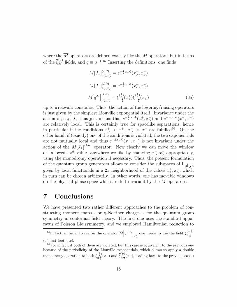
where the M operators are defined exactly like the M operators, but in terms

of the ξ(J)

M fields, and q ≡ q−1.15 Inserting the definitions, one finds

M [J+](LR)

x+>

,x−

>

= e−1

2α−Φ(x+

>, x−>)

M [J−](LR)

x+<

,x−

<

= e−1

2α−Φ(x+

<, x−<)

M[

qJ3

](LR)

x+>,x−

>

= ξ( 1

2)

− 1

2

(x+>)ξ

( 1

2)

− 1

2

(x−>) (35)

up to irrelevant constants. Thus, the action of the lowering/raising operatorsis just given by the simplest Liouville exponential itself! Invariance under theaction of, say, J+ thus just means that e−

1

2α−Φ(x+

>, x−>) and e−Jα−Φ(x+, x−)

are relatively local. This is certainly true for spacelike separations, hencein particular if the conditions x+

> > x+, x−> > x− are fulfilled16. On theother hand, if (exactly) one of the conditions is violated, the two exponentialsare not mutually local and thus e−Jα−Φ(x+, x−) is not invariant under the

action of the M [J±](LR) operator. Now clearly we can move the windowof ”allowed” x± values anywhere we like by changing x+

>, x−> appropriately,

using the monodromy operation if necessary. Thus, the present formulationof the quantum group generators allows to consider the subspaces of Γphysgiven by local functionals in a 2π neighborhood of the values x+

>, x−>, which

in turn can be chosen arbitrarily. In other words, one has movable windowson the physical phase space which are left invariant by the M operators.

7 Conclusions

We have presented two rather different approaches to the problem of con-structing moment maps - or q-Noether charges - for the quantum groupsymmetry in conformal field theory. The first one uses the standard appa-ratus of Poisson Lie symmetry, and we employed Hamiltonian reduction to

15In fact, in order to realize the operator M[

q−J3

]

x−

>

one needs to use the field ξ(− 1

2)

+ 12

(cf. last footnote).16 (or in fact, if both of them are violated; but this case is equivalent to the previous one

because of the periodicity of the Liouville exponentials, which allows to apply a double

monodromy operation to both ξ( 12)

±12

(x+) and ξ( 12)

±12

(x−), leading back to the previous case.)

18

obtain the moment map for Liouville theory from the known result for theWZW case. Our analysis was obviously incomplete as we presented only theclassical moment map. However, it is conceptually clear how to extend theanalysis to the quantum case and one expects no major technical obstacles;work on this is in progress [13]. Furthermore, an extension to general Todatheories seems both desirable and feasible.

On the other hand, in the ”intrinsic” approach working on the physicalphase space we were able to obtain a realization directly on the quantumlevel. However, this approach, which starts from a ”phenomenological” ob-servation on the structure of the R matrix, is conceptually still much less un-derstood. Its most striking feature is perhaps the position dependence of thegenerators, which suggests an embedding into a Kac-Moody type structure,though of course Liouville theory a priori just has a global SL(2) symmetry.It is intriguing that in this way one can realize a kind of BRST transforma-tions on a gauge-fixed theory without extending the phase space. Clearly, itis important to understand better the deeper meaning of this new ”weak”symmetry of the physical phase space, which leaves freely movable parts ofit invariant but never all of it. We remark that the construction can be ex-tended to Uq(sl(2)) ⊗ Uq(sl(2)) [12], where q is the deformation parameterwhich corresponds to the second screening charge α+. This symmetry is wellknown within the description of minimal models [16], where only half-integerpositive spins are relevant, but much less in the context of arbitrary spins asrequired for Liouville theory.

In ref. [14], it was shown how the second approach can also be formu-lated directly in the Bloch wave (ψ) basis, which is closely related to thestandard Coulomb gas picture of conformal field theories. Remarkably, inthis realization one finds a hidden Uq(sl(2)) × Uq(sl(2)) symmetry 17 witha nonstandard coproduct structure and an additional constraint, which de-scribes the symmetries of the Bloch wave operator algebra in the same wayas the M operators did for the ξ

(J)M fields.

Acknowledgements: The work contained in section 5 has been done incollaboration with C. Klimcik, while the results in section 6 were obtainedtogether with E. Cremmer and J.-L. Gervais. I would like to thank all ofthem for a fruitful collaboration, and B. Jurco and A. Alekseev for many

17already in the case of one screening charge !

19

helpful discussions.

References

[1] A. Alekseev, F. Faddeev, M. Semenov-Tian-Shanskii, A. Volkov, CERN-TH-5981-91, Jan. 1991. K. Gawedzki, ”Quantum Group Symmetriesin Conformal Field Theory”, Kyoto 1992 proceedings, Quantum andNoncommutative Analysis, p. 239; hep-th/9210100.

[2] O. Babelon, Phys. Lett. B215 (1988) 523.

[3] J.-L. Gervais, Comm. Math. Phys. 130 (1990) 257.

[4] L. Faddeev, N. Reshetikhin, L. Takhtadzhian, ”Quantization of LieGroups and Lie Algebras”, LOMI-E-87, 1987.

[5] F. Falceto, K. Gawedzki, lectures at the XXVIIIth Karpacz winterschool, Feb. 1992; J. Geom. Phys. 11 (1993) 251.

[6] J.-L. Gervais, J. Schnittger, Nucl. Phys. B431 (1994) 273.

[7] J.-L. Gervais, Nucl. Phys. B391 (1993) 287.

[8] A. Alekseev, I. Todorov, Nucl. Phys. B421 (1993) 413.

[9] J. Balog, L. Feher, P. Forgacs, L. O’Raifeartaigh, A. Wipf, pl B227,1989, 214. M. Bershadsky, Comm. Math. Phys. 139 (1991) 71.

[10] O. Babelon, ”From Integrable to Conformal Field Theory”, Lecturesgiven at 20th Int. GIFT seminar, Jaca, Spain, June 1989; GIFT seminar1989, p.1 and PAR-LPTHE-89-29, June 1989.

[11] J.-L. Gervais, A. Neveu, Nucl. Phys. B238 (1984) 125.

[12] E. Cremmer, J.-L. Gervais, J. Schnittger, Comm. Math.

Phys. 178 (1996) 147.

[13] C. Klimcik, J. Schnittger, work in progress.

20

[14] E. Cremmer, J.-L. Gervais, J. Schnittger, ”Hidden Uq(sl(2)) ⊗Uq(sl(2)) Quantum Group Symmetry in Two-Dimensional Gravity”,hep-th/9604131.

[15] E. Cremmer, J.-L. Gervais, J.-F. Roussel, Comm. Math.

Phys. 161 (1994) 597.

[16] L. Alvarez-Gaume, C. Gomez, G. Sierra, Nucl. Phys. B319 (1989) 155.

[17] O. Babelon, D. Bernard, Comm. Math. Phys. 149 (1992) 279; Phys.

Lett. B260 (1991) 81.

21