
CONFORMAL ANOMALY DETECTION - DiVA portal
206
DOCTORAL DISSERTATION CONFORMAL ANOMALY DETECTION Detecting abnormal trajectories in surveillance applications RIKARD LAXHAMMAR Informatics
-
Upload
khangminh22 -
Category
Documents
-
view
4 -
download
0
Transcript of CONFORMAL ANOMALY DETECTION - DiVA portal

D O C T O R A L D I S S E R T A T I O N
CONFORMAL ANOMALY DETECTION Detecting abnormal trajectories in surveillance applications
RIKARD LAXHAMMAR Informatics


CONFORMAL ANOMALY DETECTION
Detecting abnormal trajectories in surveillance applications


DOCTOR AL DISSERTATION
CONFORMAL ANOMALY DETECTION Detecting abnormal trajectories in surveillance applications
RIKARD LAXHAMMAR Informatics

This research has been supported by:
Rikard Laxhammar, 2014
Title: Conformal Anomaly Detection Detecting abnormal trajectories in surveillance applications
University of Skövde 2014, Sweden
www.his.se
Printer: Runit AB, Skövde
ISBN 978-91-981474-2-1 Dissertation Series, No. 3 (2014)

Abstract
Human operators of modern surveillance systems are confronted with an increas-ing amount of trajectory data from moving objects, such as people, vehicles, ves-sels, and aircraft. A large majority of these trajectories reflect routine traffic andare uninteresting. Nevertheless, some objects are engaged in dangerous, illegal orotherwise interesting activities, which may manifest themselves as unusual andabnormal trajectories. These anomalous trajectories can be difficult to detect byhuman operators due to cognitive limitations.
In this thesis, we have studied algorithms for the automated detection of anom-alous trajectories in surveillance applications. The main results and contributionsof the thesis are two-fold. Firstly, we propose and discuss a novel approach for an-omaly detection, called conformal anomaly detection, which is based on conformalprediction (Vovk et al.). In particular, we propose two general algorithms for an-omaly detection: the conformal anomaly detector (CAD) and the computationallymore efficient inductive conformal anomaly detector (ICAD). A key property ofconformal anomaly detection, in contrast to previous methods, is that it provides awell-founded approach for the tuning of the anomaly threshold that can be directlyrelated to the expected or desired alarm rate. Secondly, we propose and analyse twoparameter-light algorithms for unsupervised online learning and sequential detec-tion of anomalous trajectories based on CAD and ICAD: the sequential Hausdorffnearest neighbours conformal anomaly detector (SHNN-CAD) and the sequentialsub-trajectory local outlier inductive conformal anomaly detector (SSTLO-ICAD),which is more sensitive to local anomalous sub-trajectories.
We have implemented the proposed algorithms and investigated their classi-fication performance on a number of real and synthetic datasets from the videoand maritime surveillance domains. The results show that SHNN-CAD achievescompetitive classification performance with minimum parameter tuning on videotrajectories. Moreover, we demonstrate that SSTLO-ICAD is able to accuratelydiscriminate realistic anomalous vessel trajectories from normal background traffic.
Keywords: Anomaly detection, conformal prediction, trajectory analysis, videosurveillance, maritime surveillance.
I


Sammanfattning
Operatörer av moderna övervakningssystem ställs inför en allt större mängd data iform av rörelsebanor från olika typer av objekt, t.ex. människor, fordon, fartyg ochflygplan. En stor majoritet av dessa rörelsebanor motsvarar rutinmässig trafik ochär ointressant. Några av objekten är dock involverade i farlig, olovlig eller på annatsätt intressant aktivitet, vilket kan yttra sig i form av ovanliga rörelsebanor. Sådanaavvikande rörelsebanor kan vara svåra att uppräcka för en mänsklig operatör p.g.a.kognitiva begränsningar, och det finns därför ett behov av ett automatiserat stöd.
I denna avhandling studeras algoritmer for automatiserad upptäckt av avvi-kande rörelsebanor inom övervakningstillämpningar. De huvudsakliga resultatenoch bidragen hos avhandlingen är tvåfaldiga. För det första, föreslås, analyserasoch diskuteras en ny ansats till avvikelsedetektion kallad conformal anomaly de-tection, som är baserad på conformal prediction (Vovk et al.). Framförallt föreslåstvå generella algoritmer för avvikelsedetektion: conformal anomaly detector (CAD)och inductive conformal anomaly detector (ICAD), där den senare är beräknings-mässigt mer effektiv. En nyckelegenskap hos conformal anomaly detection är attdenna metod, till skillnad från tidigare metoder, erbjuder en teoretiskt välgrun-dad ansats till tröskelsättning, som direkt kan relateras till önskad eller förväntadlarmfrekvens. För det andra, förelås och analyseras två parameterlätta algorit-mer, baserade på CAD och ICAD, för oövervakad och inkrementell inlärning samtsekventiell detektion av avvikande banor: Sequential Hausdorff nearest neighboursconformal anomaly detector (SHNN-CAD) och sequential sub-trajectory local outli-er inductive conformal anomaly detector (SSTLO-ICAD). Den senare är känsligareför lokala avvikelser hos rörelsebanorna.
Vi implementerar och undersöker klassificeringsprestanda hos de två föreslagnaalgoritmerna på ett antal verkliga och syntetiska datamängder inom videoövervak-ning och sjöövervakning. Resultaten visar att SHNN-CAD uppnår konkurrenskraf-tig prestanda med minimal parametertrimning på videodata. Vidare demonstrerarvi att SSTLO-ICAD med hög noggrannhet kan särskilja realistiskt simulerade far-tygsavvikelser från verkliga fartygsrörelser som motsvarar normal bakgrundstrafik.
III


Acknowledgments
First and foremost, I would like to thank my main supervisor, Göran Falkman.You have shown great commitment to my research project at all times, and youradvice and support have been invaluable to me. There were many times when Ifelt discouraged and resigned before our supervision meetings. Yet, on each suchoccasion, I left the meeting feeling relieved and encouraged. I would also like toexpress my sincerest gratitude to Klas Wallenius, who has been my mentor atSaab. Without your support and commitment, this research project would neverhave been realised in the first place. Your advice and feedback have been highlyimportant to my research and the writing of this thesis.
This research has been supported by my employer Saab AB, and I am verygrateful and proud of the unique opportunity they have offered me. I would liketo extend special thanks to Egils Sviestins at Saab, the co-author of one of mypapers, who has given me valuable feedback on my research, including a draft ofthis thesis and all my published papers. Other Saab employees, who have givenme feedback, and with whom I have had many interesting discussions, includeMattias Björkman, Thomas Kronhamn, Martin Smedberg, and Håkan Warston.
I am also very thankful to my current and former colleagues of the GSA re-search group at the University of Skövde: Christoffer Brax, who kindly providedthe maritime dataset with labelled anomalies, and with whom I have co-authoredtwo papers and had many interesting discussions; Lars Niklasson, who has been myco-advisor; Fredrik Johansson, Anders Dahlbom, Maria Riveiro, Tina Erlandsson,and Tove Helldin. I appreciate not only your feedback and our scientific discus-sions, but also our social intercourse during lunches, coffee breaks and other socialactivities. I would also like to acknowledge Volodya Vovk, at the Royal Hollo-way University of London, for giving me valuable feedback regarding my workon conformal anomaly detection, and Stefan Arnborg, at the Royal Institute ofTechnology in Stockholm, who first introduced me to the exciting research area ofconformal prediction.
Last, but not least, I would like to thank my beloved Kajsa, for always beingthere and for putting up with, at times, an absent-minded researcher at home.
V


List of Publications
I. Laxhammar, R. (2014) Anomaly Detection. To appear in Conformal Pre-diction for Reliable Machine Learning: Theory, Adaptations, and Applica-tions (eds. Balasubramanian, V., Ho, S. and Vovk, V.), Elsevier InsightSeries, Morgan-Kaufmann Publishers, 2014.
II. Laxhammar, R. and Falkman, G. (2013) Inductive Conformal AnomalyDetection for Sequential Detection of Anomalous Sub-Trajectories. In An-nals of Mathematics and Artificial Intelligence: Special Issue on ConformalPrediction and its Applications, September 2013.
III. Laxhammar, R. and Falkman, G. (2013) Online Learning and Sequen-tial Anomaly Detection in Trajectories. In IEEE Transactions on PatternAnalysis and Machine Intelligence, volume 99, PrePrints, September 2013.
IV. Laxhammar, R. and Falkman, G. (2012) Online Detection of AnomalousSub-Trajectories - A Sliding Window Approach Based on Conformal An-omaly Detection and Local Outlier Factor. In Proceedings of the AIAI 2012Workshop on Conformal Prediction and its Applications, volume 382 of IFIPAdvances in Information and Communication Technology, pages 192–202,Berlin, 2012.
V. Holst, A., Bjurling, B., Ekman, J., Rudström, Å., Wallenius, K., Laxham-mar, R., Björkman, M., Fooladvandi, F. and Trönninger, J. (2012) A JointStatistical and Symbolic Anomaly Detection System Increasing Performancein Maritime Surveillance. In Proceedings of the 15th International Confer-ence on Information Fusion, Singapore, July 2012.
VI. Laxhammar, R. (2011) Anomaly Detection in Trajectory Data for Surveil-lance Applications. Licentiate Thesis, Örebro University, 2011.
VII. Laxhammar, R. and Falkman, G. (2011) Sequential Conformal AnomalyDetection in Trajectories based on Hausdorff Distance. In Proceedings of the14th International Conference on Information Fusion, Chicago, USA, July2011.
VII

VIII. Laxhammar, R. and Falkman, G. (2010) Conformal Prediction forDistribution-Independent Anomaly Detection in Streaming Vessel Data. InProceedings of the First International Workshop on Novel Data Stream Pat-tern Mining Techniques (ACM), Washington D.C., USA, July 2010.
IX. Laxhammar, R., Falkman, G. and Sviestins, E. (2009) Anomaly Detectionin Sea Traffic - a Comparison of the Gaussian Mixture Model and the KernelDensity Estimator. In Proceedings of the 12th International Conference onInformation Fusion, Seattle, USA, July 2009.
X. Brax, C., Niklasson, L. and Laxhammar, R. (2009) An ensemble approachfor increased anomaly detection performance in video surveillance data. InProceedings of the 12th International Conference on Information Fusion,Seattle, USA, July 2009.
XI. Brax, C., Laxhammar, R. and Niklasson, L. (2008) Approaches for detect-ing behavioural anomalies in public areas using video surveillance data. InProceedings of SPIE Electro-Optical and Infrared Systems: Technology andApplications V, Cardiff, Wales, September 2008.
XII. Laxhammar, R. (2008) Anomaly detection for sea surveillance. In Proceed-ings of the 11th International Conference on Information Fusion, Cologne,Germany, July 2008.
VIII

Abbreviations and Acronyms
AIS Automatic identification system
AUC Area under the receiver operating characteristics curve
CAD Conformal anomaly detector
CP Conformal prediction
DH-kNN-NCM Directed Hausdorff k -nearest neighbours nonconformitymeasure
DTW Dynamic time warping
ED Euclidean distance
EM Expectation-maximization
GMM Gaussian mixture model
HD Hausdorff distance
HMM Hidden Markov model
ICAD Inductive conformal anomaly detector
ICP Inductive conformal prediction
IID Independent and identically distributed
KDE Kernel density estimation
LCSS Longest common sub-sequence
LOF Local outlier factor
MAP Maximum a posterior
ML Maximum likelihood
NCM Nonconformity measure
IX

pAUC Partial area under the receiver operating characteristics curve
PDF Probability density function
ROC Receiver operating characteristics
SBAD State-based anomaly detection
SHNN-CAD Sequential Hausdorff nearest neighbours conformal anomalydetector
SOM Self-organising map
SSTLO-ICAD Sequential sub-trajectory local outlier inductive conformalanomaly detector
SSTLO-NCM Sequential sub-trajectory local outlier nonconformity measure
SVM Support Vector Machine
X

List of Symbols
δH Undirected Hausdorff distance−→δH Directed Hausdorff distance
A Nonconformity measure (NCM)
B Multi-set
ε Significance level
p p-value
α Nonconformity score
k Number of nearest neighbours
w Window (sub-trajectory) length
XI


Contents
1 Introduction 11.1 Research Question and Objectives . . . . . . . . . . . . . . . . . . 41.2 Research Methodology . . . . . . . . . . . . . . . . . . . . . . . . . 41.3 Scientific Contributions . . . . . . . . . . . . . . . . . . . . . . . . 5
1.3.1 Anomaly Detection . . . . . . . . . . . . . . . . . . . . . . . 51.3.2 Anomalous Trajectory Detection . . . . . . . . . . . . . . . 61.3.3 Conformal Prediction . . . . . . . . . . . . . . . . . . . . . 7
1.4 Publications . . . . . . . . . . . . . . . . . . . . . . . . . . . . . . . 81.5 Thesis Outline . . . . . . . . . . . . . . . . . . . . . . . . . . . . . 13
2 Background 152.1 Anomaly Detection . . . . . . . . . . . . . . . . . . . . . . . . . . . 15
2.1.1 General Aspects of Anomaly Detection . . . . . . . . . . . . 162.1.2 Statistical Anomaly Detection . . . . . . . . . . . . . . . . . 202.1.3 Other Anomaly Detection Algorithms . . . . . . . . . . . . 25
2.2 Anomalous Trajectory Detection . . . . . . . . . . . . . . . . . . . 282.2.1 Video Surveillance . . . . . . . . . . . . . . . . . . . . . . . 292.2.2 Maritime Surveillance . . . . . . . . . . . . . . . . . . . . . 33
3 The Research Gap 373.1 Anomaly Detection . . . . . . . . . . . . . . . . . . . . . . . . . . . 37
3.1.1 Inaccurate Statistical Models . . . . . . . . . . . . . . . . . 373.1.2 Parameter-laden Algorithms . . . . . . . . . . . . . . . . . . 393.1.3 Ad-hoc Anomaly Thresholds and High False Alarm Rates . 39
3.2 Anomalous Trajectory Detection . . . . . . . . . . . . . . . . . . . 413.2.1 Offline Learning . . . . . . . . . . . . . . . . . . . . . . . . 413.2.2 Offline Anomaly Detection . . . . . . . . . . . . . . . . . . 413.2.3 Insensitivity to Local Sub-Trajectory Anomalies . . . . . . 42
3.3 Identification of Key Properties . . . . . . . . . . . . . . . . . . . . 43
XIII

CONTENTS
4 Conformal Anomaly Detection 454.1 Preliminaries: Conformal Prediction . . . . . . . . . . . . . . . . . 454.2 Conformal Prediction for Multi-Class Anomaly Detection . . . . . 48
4.2.1 A Nonconformity Measure for Multi-class Anomaly Detection 484.3 Conformal Anomaly Detection . . . . . . . . . . . . . . . . . . . . 50
4.3.1 The Conformal Anomaly Detector . . . . . . . . . . . . . . 504.3.2 Offline and Online Conformal Anomaly Detection . . . . . 524.3.3 Unsupervised and Semi-Supervised Conformal Anomaly De-
tection . . . . . . . . . . . . . . . . . . . . . . . . . . . . . . 524.3.4 Importance of the Nonconformity Measure . . . . . . . . . 534.3.5 Tuning of the Anomaly Threshold . . . . . . . . . . . . . . 54
4.4 Inductive Conformal Anomaly Detection . . . . . . . . . . . . . . . 544.4.1 Offline and Semi-Offline Inductive Conformal Anomaly De-
tection . . . . . . . . . . . . . . . . . . . . . . . . . . . . . . 554.4.2 Online Inductive Conformal Anomaly Detection . . . . . . 56
4.5 Summary . . . . . . . . . . . . . . . . . . . . . . . . . . . . . . . . 58
5 Sequential Detection of Anomalous Trajectories 595.1 Sequential Conformal Anomaly Detection . . . . . . . . . . . . . . 59
5.1.1 Preliminaries: Hausdorff Distance . . . . . . . . . . . . . . 605.1.2 A Nonconformity Measure for Examples Represented as Sets
of Points . . . . . . . . . . . . . . . . . . . . . . . . . . . . . 605.1.3 The Sequential Hausdorff Nearest Neighbours Conformal An-
omaly Detector . . . . . . . . . . . . . . . . . . . . . . . . . 625.1.4 Discussion . . . . . . . . . . . . . . . . . . . . . . . . . . . . 65
5.2 Empirical Investigations . . . . . . . . . . . . . . . . . . . . . . . . 665.2.1 Accuracy of Trajectory Outlier Measures . . . . . . . . . . 675.2.2 Unsupervised Online Learning and Sequential Anomaly De-
tection Performance . . . . . . . . . . . . . . . . . . . . . . 705.2.3 Discussion . . . . . . . . . . . . . . . . . . . . . . . . . . . . 74
5.3 Summary . . . . . . . . . . . . . . . . . . . . . . . . . . . . . . . . 78
6 Sequential Detection of Anomalous Sub-Trajectories 816.1 A Nonconformity Measure for the Sequential Detection of Local
Anomalous Sub-Trajectories . . . . . . . . . . . . . . . . . . . . . . 816.1.1 Preliminaries: Local Outlier Factor . . . . . . . . . . . . . . 826.1.2 The Sequential Sub-Trajectory Local Outlier Nonconformity
Measure . . . . . . . . . . . . . . . . . . . . . . . . . . . . . 846.2 The Sequential Sub-Trajectory Local Outlier Inductive Conformal
Anomaly Detector . . . . . . . . . . . . . . . . . . . . . . . . . . . 906.3 Empirical Investigations in the Maritime Domain . . . . . . . . . . 90
6.3.1 Preliminary Investigations . . . . . . . . . . . . . . . . . . . 916.3.2 Empirical Alarm Rate . . . . . . . . . . . . . . . . . . . . . 976.3.3 Detection Delay: Simulated Anomalies . . . . . . . . . . . . 986.3.4 Classification Performance: Realistic Anomalies . . . . . . . 105
XIV

CONTENTS
6.4 Summary . . . . . . . . . . . . . . . . . . . . . . . . . . . . . . . . 129
7 Conclusion 1337.1 Contributions . . . . . . . . . . . . . . . . . . . . . . . . . . . . . . 133
7.1.1 Research Question . . . . . . . . . . . . . . . . . . . . . . . 1387.2 Future Work . . . . . . . . . . . . . . . . . . . . . . . . . . . . . . 1417.3 Generalisation . . . . . . . . . . . . . . . . . . . . . . . . . . . . . . 1427.4 Final Remarks . . . . . . . . . . . . . . . . . . . . . . . . . . . . . 143
A Performance Results: Realistic Maritime Anomalies 145A.1 Circle and Land . . . . . . . . . . . . . . . . . . . . . . . . . . . . . 146A.2 Missed Turn . . . . . . . . . . . . . . . . . . . . . . . . . . . . . . . 148A.3 Unexpected Stop . . . . . . . . . . . . . . . . . . . . . . . . . . . . 150A.4 Unusual Speed . . . . . . . . . . . . . . . . . . . . . . . . . . . . . 152A.5 Strange Manoeuvres . . . . . . . . . . . . . . . . . . . . . . . . . . 154A.6 Large Vessel in Unusual Location . . . . . . . . . . . . . . . . . . . 156A.7 Unexpected Vessel Type/Behaviour . . . . . . . . . . . . . . . . . . 158A.8 Overall Performance . . . . . . . . . . . . . . . . . . . . . . . . . . 160
References 162
XV


List of Figures
3.1 Estimated PDF for vessel position using GMM and EM . . . . . . 383.2 Illustration of global vs. local trajectory anomaly . . . . . . . . . . 43
4.1 Problem with previous k -nearest neighbours nonconformity meas-ure for anomaly detection . . . . . . . . . . . . . . . . . . . . . . . 49
5.1 Illustration of directed Hausdorff distance between two curves . . . 615.2 Plot of trajectories from the first synthetic dataset . . . . . . . . . 685.3 Plot of trajectories from the first dataset of recorded video trajectories 695.4 Plot of trajectories from the second dataset of recorded video tra-
jectories . . . . . . . . . . . . . . . . . . . . . . . . . . . . . . . . . 705.5 Plot of trajectories from the second synthetic dataset . . . . . . . . 725.6 Plots of sensitivity and precision dependent on size of the training
set during online learning and sequential anomaly detection . . . . 755.7 Plot of the mean detection delay dependent on the size of the train-
ing set during online learning and sequential anomaly detection . . 765.8 Histogram of the empirical alarm rate for the unsupervised online
SHNN-CAD . . . . . . . . . . . . . . . . . . . . . . . . . . . . . . . 77
6.1 Illustration of the local density problem . . . . . . . . . . . . . . . 836.2 Illustration of the smoothening effect of the reachability distance . 856.3 Illustration of top three anomalous vessel trajectories according to
SSTLO-NCM with w = 6 and k = 5 . . . . . . . . . . . . . . . . . 936.4 Illustration of top three anomalous vessel trajectories according to
SSTLO-NCM with w = 6 and k = 2 . . . . . . . . . . . . . . . . . 946.5 Illustration of top three anomalous vessel trajectories according to
SSTLO-NCM with w = 61 and k = 5 . . . . . . . . . . . . . . . . . 956.6 Illustration of top three anomalous vessel trajectories according to
SSTLO-NCM with w = 61 and k = 2 . . . . . . . . . . . . . . . . . 966.7 Histograms of the empirical alarm rates for different parameter val-
ues of the semi-offline SSTLO-ICAD . . . . . . . . . . . . . . . . . 996.8 Histograms of the empirical alarm rates for different parameter val-
ues of the alternative online SSTLO-ICAD . . . . . . . . . . . . . . 100
XVII

LIST OF FIGURES
6.9 Plot of the accumulated nr of anomalous trajectories detected as afunction of the nr of trajectories . . . . . . . . . . . . . . . . . . . 101
6.10 Plot of extracted vessel trajectories from port area of Gothenburg . 1026.11 Plot of simulated anomalous vessel trajectories in port area of Gothen-
burg . . . . . . . . . . . . . . . . . . . . . . . . . . . . . . . . . . . 1036.12 Geographical coverage of the dataset of recorded vessel trajectories
and realistic anomalies. . . . . . . . . . . . . . . . . . . . . . . . . 1096.13 Plot of vessel trajectories from training set and the normal test set 1106.14 Plot of maritime anomalies: vessels that circle and land. . . . . . . 1146.15 Plot of maritime anomalies: vessels that miss a turn. . . . . . . . . 1156.16 Plot of maritime anomalies: unexpected stops. . . . . . . . . . . . 1166.17 Plot of a maritime anomalies: unusual speed . . . . . . . . . . . . 1176.18 Plot of a maritime anomaly: strange manoeuvres. . . . . . . . . . . 1186.19 Plot of maritime anomalies: large vessels in unusual locations. . . . 1196.20 Plot of maritime anomalies: passenger vessels behaving strangely. . 1206.21 Plot of maritime anomalies: tankers behaving strangely. . . . . . . 1216.22 Example of ROC curves. . . . . . . . . . . . . . . . . . . . . . . . . 124
XVIII

List of Tables
1.1 Overview: research objectives, publications, thesis chapters . . . . 14
5.1 Accuracy on the first dataset of synthetic trajectories . . . . . . . . 685.2 Accuracy on the second dataset of recorded video trajectories . . . 715.3 F1-score and detection delay on the second dataset of synthetic
trajectories . . . . . . . . . . . . . . . . . . . . . . . . . . . . . . . 74
6.1 Mean detection delay on simulated anomalous vessel trajectories . 1066.2 Median detection delay on simulated anomalous vessel trajectories 1076.3 Overview of the different maritime anomaly classes. . . . . . . . . 1126.4 Average classification performance of SSTLO-NCM on set of mari-
time anomalies for different values of k. . . . . . . . . . . . . . . . 1266.5 Average classification performance of SSTLO-NCM on set of mari-
time anomalies for different sub-trajectory lengths. . . . . . . . . . 1266.6 pAUC for SSTLO-NCM and discords based on spatial trajectory
representation. . . . . . . . . . . . . . . . . . . . . . . . . . . . . . 1276.7 pAUC for SSTLO-NCM and discords based on velocity vector tra-
jectory representation. . . . . . . . . . . . . . . . . . . . . . . . . . 1276.8 Sensitivity and mean detection delay on each maritime anomaly
class for SSTLO-NCM, discords and SBAD. . . . . . . . . . . . . . 129
7.1 Overview of the identified key properties and the proposed and eval-uated algorithms in the thesis. . . . . . . . . . . . . . . . . . . . . 139
XIX


List of Algorithms
4.1 Conformal predictor . . . . . . . . . . . . . . . . . . . . . . . . . . 464.2 The Conformal Anomaly Detector (CAD) . . . . . . . . . . . . . . 514.3 The Inductive Conformal Anomaly Detector (ICAD) . . . . . . . . 555.1 The Sequential Hausdorff Nearest Neighbours Conformal Anomaly
Detector (SHNN-CAD) . . . . . . . . . . . . . . . . . . . . . . . . 646.1 K -d tree based sequential sub-trajectory local outlier nonconformity
measure (SSTLO-NCM) . . . . . . . . . . . . . . . . . . . . . . . . 876.2 Sub-trajectory neighbourhood algorithm . . . . . . . . . . . . . . . 88
XXI


Chapter 1
Introduction
Anomalous behaviour, also referred to as strange, suspicious, unusual, novel orunexpected behaviour, may indicate interesting objects or events in a wide vari-ety of domains. An important example is surveillance in the military and civilsecurity domains, where there is a clear trend towards more and more advancedsensor systems producing huge amounts of geo-spatial and temporal trajectorydata from moving objects, including people, vehicles, vessels and aircraft. Inmaritime surveillance, anomalous vessel trajectories corresponding to unexpec-ted stops, deviations from standard routes, speeding, traffic direction violationsetc., may indicate threats and dangers related to smuggling, command of a vesselwhile drunk1, collisions (Danish Maritime Authority, 2003), grounding (SwedishMaritime Safety Inspectorate, 2004), terrorism2, hijacking3, piracy4 etc. In videosurveillance of on-land activities, anomalous trajectories may indicate illegal andadverse activity related to personal assault, robbery, burglary, infrastructural sab-otage etc. The timely detection of these relatively infrequent events is criticalfor enabling pro-active measures to be taken and requires constant analysis of alltrajectories. This is typically a significant challenge for human analysts due toinformation overload, fatigue and inattention (Riveiro, 2011). At any one timein the Baltic sea, for example, there are typically 3000–4000 commercial vesselsbeing monitored by only a few human analysts5. Hence, there is need of a systemthat supports the automated analysis of all collected trajectory data and alertshuman analysts of potentially interesting targets. In this thesis, we are concernedwith the problem of the automated detection of anomalous trajectories in surveil-lance applications. The main contribution of our work is the proposal, analysisand empirical investigations of algorithms appropriate for the online detection of
1http://www.swedishwire.com/economy/5738-drunk-captain-runs-aground-in-sweden2http://www.globalsecurity.org/security/profiles/uss_cole_bombing.htm3http://news.bbc.co.uk/2/hi/uk_news/8196640.stm4http://en.wikipedia.org/wiki/Piracy_in_Somalia5http://www.idg.se/2.1085/1.376546/sjobasis-battre-an-stalmannens-
rontgensyn?utm_source=tip-friend&utm_medium=email
1

Chapter 1. Introduction
anomalous trajectories during surveillance operations.
In the research fields of data fusion (Hall and McMullen, 2004) and data min-ing (Tan et al., 2006), various computational methods that support surveillanceanalysts in detecting abnormal and interesting behaviour have been proposed(Riveiro, 2011; Brax, 2011). According to Rhodes (2009), “timely identificationand assessment of anomalous activity within an area of interest is an increasinglyimportant capability — one that falls under the enhanced situation awareness ob-jective of higher-level [data] fusion”. Signature-based methods (Patcha and Park,2007) assume that specific models for interesting behaviour, such as rules andtemplates, can be defined a priori and used for automated pattern recognitionin new data. Such models are constructed according to two main knowledge ex-traction strategies: incorporation of human expert knowledge regarding suspiciousand interesting behaviours (Edlund et al., 2006; Dahlbom et al., 2009) and su-pervised learning from labelled data of interesting and non-interesting behaviour(Fooladvandi et al., 2009) using methods from machine learning (Mitchell, 1997).Of particular interest is a general machine learning method called conformal pre-diction (Vovk et al., 2005), which provides reliable and well-calibrated measuresof confidence in the predictions made by traditional machine learning algorithms.The system’s confidence in predicting that a particular behaviour is interesting, ornon-interesting, may be important information for determining whether the situ-ation needs to be further examined by a human analyst. However, it has beenargued that signature-based methods are not sufficient, since accurate models ofall possible behaviour of interest cannot be acquired in practice (Patcha and Park,2007). This is mainly due to the lack of expert knowledge and annotated datathat covers the full spectrum of interesting behaviour, as well as practical en-gineering difficulties in encoding expert knowledge. According to Kraiman et al.(2002), “there is a need for robust, non-template-based processing techniques thatmonitor large tracking and surveillance datasets”. It has also been argued that theanalysis should be focused towards detecting “strange” and abnormal patterns thatdeviate from the expected or “normal” patterns. Such approaches, typically re-ferred to as anomaly, novelty or outlier detection methods (Chandola et al., 2009),benefit from the fact that there is usually large amounts of historical data, whichcan be exploited to learning normal behaviour. In contrast to signature-basedapproaches, these methods require less prior knowledge regarding the abnormal orinteresting behaviour. Nevertheless, signature-based methods and anomaly detec-tion methods complement each other and should be combined in order to achieveimproved overall performance (Holst et al., 2012). The remainder of the thesis isonly concerned with anomaly detection methods for detecting anomalous traject-ories.
A key issue when designing an anomaly detector is how to represent the datain which anomalies can be found. Some anomaly detection methods assume thatdata, in our case trajectories, is represented as points in a fixed-dimensional featurespace. This implies that a fixed number of features, e.g., the position at a fixednumber of points in time, has to be extracted from each trajectory or trajectory
2

segment. Other methods only assume that a similarity or dissimilarity measureis defined for pairs of trajectories or trajectory segments. The choice of featuresor similarity or dissimilarity measure essentially determines the type of anomaliesthat can be detected and is therefore very important.
Most of the previously proposed algorithms are essentially designed for offlineanomaly detection in trajectory databases. Hence, they typically assume that thecomplete trajectory has been observed before it is classified as anomalous or not.This is a limitation in surveillance applications since it delays anomaly alarmsand, thus, the ability to react to impending events. In contrast, algorithms forsequential anomaly detection allow detection in incomplete trajectories (Morrisand Trivedi, 2008a), e.g., real-time detection of anomalous trajectories as theyevolve. Moreover, learning in previously proposed algorithms is usually offline,i.e., fixed model parameters and thresholds are estimated or tuned once basedon a batch of historical data. Thus, once the anomaly detector is deployed inthe current application, it cannot leverage on new training data that is collectedincrementally. The need for online learning in the surveillance domain has beenidentified and discussed by Piciarelli and Foresti (2006) and Rhodes et al. (2007).
Generally, anomaly detection algorithms require the careful setting of multipleapplication specific parameters in order to achieve good performance; anomaloustrajectory detection is no exception to this. According to Markou and Singh(2003a), “an [anomaly] detection method should aim to minimise the number ofparameters that are user set”. Indeed, Keogh et al. (2007) argue that most datamining algorithms are more or less parameter-laden, which increases the risk ofoverfitting the model to the training data and makes implementing the algorithmsmore difficult. A central parameter of most anomaly detection algorithms is theanomaly threshold, which regulates the trade-off between the sensitivity to trueand interesting anomalies, and the rate of false alarms, i.e., detected anomaliesthat correspond to normal and uninteresting data. While achieving high sensitivityis important, it has been argued that the false alarm rate is the critical factor forthe performance of an anomaly detection system (Axelsson, 2000; Riveiro, 2011).Indeed, Riveiro (2011) argues that a high false alarm rate “may become a nuisancefor operators who might turn [the anomaly detector] off”. In many cases, anapplication specific distance or density based threshold is used to decide whethernew data is anomalous or not. The thresholds are often not normalised and seemto lack intuition, and the procedures for setting the thresholds seem to be moreor less ad-hoc. This increases the risk of high false alarm rates due to poorlycalibrated thresholds.
Various algorithms have previously been proposed for anomalous trajectorydetection in surveillance applications, such as video surveillance and maritimesurveillance. Yet, we argue that these algorithms typically suffer from drawbacksrelated to one or more of the issues discussed above: they are designed for offlineanomaly detection in trajectory databases, they are parameter-laden and they maysuffer from high false alarm rates due to ad-hoc and poorly calibrated anomalythresholds. In this thesis, we aim to bridge this gap in the research.
3

Chapter 1. Introduction
1.1 Research Question and Objectives
Following the argumentation in the last paragraph above, the overall researchquestion of this thesis is formulated as follows:
Research Question: What are appropriate algorithms for the detection of an-omalous trajectories in surveillance applications?
In order to answer this research question, the following set of objectives are iden-tified:
O1 Review and analyse previously proposed algorithms for anomaly detectionin general and anomalous trajectory detection in particular.
O2 Identify important and desirable properties of algorithms for anomalous tra-jectory detection in surveillance applications.
O3 Propose and analyse new or updated algorithms that are more appropriatefor anomalous trajectory detection in surveillance applications.
O4 Identify appropriate performance measures for evaluating algorithms for an-omalous trajectory detection in surveillance applications.
O5 Implement the proposed algorithms and evaluate the performance of newand previous algorithms on synthetic and real trajectory datasets.
1.2 Research Methodology
In order to address the research objectives stated in Section 1.1, we adopt a numberof different research methods.
Starting with O1 and O2, we perform two literature reviews and literatureanalyses (Berndtsson et al., 2002). The first is focused on algorithms for anomalydetection in general, while the second is focused on algorithms for anomaloustrajectory in surveillance applications. An important issue when undertaking aliterature analysis is how to systematically search for previously published workthat is relevant for the current research (Berndtsson et al., 2002). Therefore, weadopt a number of different search strategies based on:
• Searching the internet in general, and in scientific databases in particular, us-ing different combinations of selected keywords, such as “anomaly detection”,“surveillance”, “trajectory data” etc.
• Browsing journals and annual proceedings of selected conferences, choosing asubset of papers for further reading based on title, abstract and/or keywords.
• Backwards citation chaining from relevant papers previously found.
In order to enable the evaluation of the proposed algorithms (O5), we develop animplementation (Berndtsson et al., 2002) for each of them in MATLAB6 or Java™.
6http://www.mathworks.com
4

1.3. Scientific Contributions
An important issue when developing an implementation of an algorithm is toensure its reliability (Berndtsson et al., 2002), i.e., the robustness and correctnessof the implementation. The algorithms implemented in MATLAB are largelybased on functions and subroutines from the standard MATLAB library and theofficial Statistics toolbox7 by MathWorks, which strengthens the reliability of theimplementations.
In order to evaluate the proposed algorithms according to the identified per-formance measures (O5) , we perform a series of experiments (Berndtsson et al.,2002) using the implementations of the corresponding algorithms and different tra-jectory datasets. Machine learning algorithms are typically evaluated by measuringtheir classification performance on a labelled dataset, which is often publicly avail-able8. However, public availability of real world surveillance data is very limiteddue to confidentiality and proprietary rights. Moreover, a real-world surveillancedataset is typically unlabelled, i.e., there is no information regarding which part ofthe data is actually normal or anomalous, and includes very few, if any, true an-omalies; this may threaten the validity and reliability of experimental results andconclusions. An alternative to real world data is to simulate data, which has theadvantages that 1) the resulting data is labelled and 2) the reproducibility of exper-iments is enhanced, under the assumption that the data can more easily be madepublicly available (downloaded) or accurately re-created given the parameters anddetails of the simulation process. The main drawback of using simulated data isthat validity or generalisability may be questioned if, e.g., the simulated anomaliesdo not reflect the actual anomalies encountered in a real surveillance application.That is, we are actually measuring performance on a different problem (detectsimulated anomalies) than the one we aim to measure (detect true anomalies). Inthis thesis, we evaluate the performance of the proposed algorithms using bothreal and simulated trajectories. Moreover, we reproduce a number of previouslypublished experiments on labelled datasets.
1.3 Scientific Contributions
This thesis is based on the author’s previously published work by the author(Section 1.4), which has been further extended with new empirical results. Themain scientific contributions of the thesis, listed below, are organised accordingto the research areas anomaly detection in general, anomalous trajectory detectionand conformal prediction:
1.3.1 Anomaly Detection• Compilation of key properties of algorithms for anomaly detection and cor-
responding limitations of previous algorithms (Section 3.1).
7http://www.mathworks.com/products/statistics/8see, e.g., the UCI Machine Learning Repository: http://archive.ics.uci.edu/ml/
5

Chapter 1. Introduction
Various strengths and weaknesses of different approaches to anomaly de-tection have previously been discussed by others (see, e.g., Chandola et al.(2009)). In this thesis, we complement previous surveys by identifying anumber of key properties of any anomaly detector and the correspondinglimitations of previously proposed algorithms in the literature. While thesekey properties have been separately identified by previous authors (see, e.g.,Keogh et al., 2007; Axelsson, 2000; Riveiro, 2011), we argue that the compil-ation and overall discussion of all these properties is a contribution in itselfto the field of anomaly detection.
• Proposal, analysis and discussion of a novel algorithmic framework, known asconformal anomaly detection, with a unique set of properties that addressesthe limitations of previous approaches (Sections 4.3 and 4.4).
The conformal anomaly detection framework is one of the main contribu-tions of the thesis. The framework addresses the limitations of previousapproaches above and supports both unsupervised and semi-supervised, off-line and online anomaly detection.
1.3.2 Anomalous Trajectory Detection
• Compilation of key properties of algorithms for anomalous trajectory detec-tion and the corresponding limitations of previous work (Section 3.2).
In this thesis, we identify and discuss key properties of any algorithm foranomalous trajectory detection. These key properties have also been beenidentified by previous authors (Lee et al., 2008; Piciarelli and Foresti, 2006);nevertheless, the compilation and overall discussion of these properties is acontribution in itself within the field of anomalous trajectory detection.
• Proposal and analysis of algorithms for the sequential detection of anomal-ous trajectories that address the above limitations (Sections 5.1.3 and 6.1).
One of the main contributions of the thesis concerns the proposal and ana-lysis of two algorithms for online learning and the sequential detection ofanomalous trajectories and sub-trajectories, respectively.
• Results and discussions regarding the classification performance on labelleddatasets of real and synthetic trajectories in the domains of video surveillance(Section 5.2) and maritime surveillance (Section 6.3).
We implement the algorithms proposed for anomalous trajectory detectionand evaluate their classification performance on labelled datasets. This isdone by reproducing previously published experiments and designing newexperiments. For comparative purposes, we also implement the discordsalgorithm (Keogh et al., 2005) and investigate its performance.
6

1.3. Scientific Contributions
1.3.3 Conformal Prediction
• Extension of the conformal prediction framework for solving the anomalydetection problem (cf. Section 1.3.1) (Chapter 4).
The conformal prediction framework was originally proposed to provide reli-able measures of confidence during supervised learning and prediction (Vovket al., 2005). In this thesis, we have extended conformal prediction to thegeneral problem of semi-supervised and unsupervised anomaly detection. Wehave a described how any conformal predictor can be adopted for multi-classanomaly detection, including a discussion of its key properties. Moreover, wehave proposed the conformal anomaly detector (CAD) and the inductive con-formal anomaly detector (ICAD), which are two general anomaly detectionalgorithms based on conformal prediction (Vovk et al., 2005) and inductiveconformal prediction (Vovk et al., 2005), respectively.
• Proposal and analysis of a novel nonconformity measure (NCM) based onthe Hausdorff distance (Alt et al., 1995) (Section 5.1.2).
The NCM is the main design parameter in conformal prediction and con-formal anomaly detection. Previously proposed NCMs (Vovk et al., 2005)assume that each example is represented as a vector in a fixed-dimensionalfeature space. This may be a limitation in applications where examples arenaturally represented as sequences or sets of data points of varying length orsize, respectively. In the thesis, we propose the directed Hausdorff k -nearestneighbours nonconformity measure (DH-kNN-NCM), which is a novel NCMdesigned for examples that are represented as sets of points. One of the keyproperties of DH-kNN-NCM is that it allows for sequential calculation ofthe preliminary nonconformity score for an incomplete example, i.e., whenonly a subset of the data points or feature values is observed. In particu-lar, we prove that the sequence of preliminary nonconformity scores increasesmonotonically as the example is updated sequentially with more data points.This property will ensure that the prediction sets of any conformal predictorbased on DH-kNN-NCM will remain valid during the sequential update of anew example.
• Proposal and analysis of a novel NCM for trajectory data based on localoutlier factor (LOF) (Breunig et al., 2000) (Section 6.1.2).
As discussed above, previous NCMs are not designed for examples represen-ted as sequences of points that are updated sequentially, such as trajectories.The DH-kNN-NCM above addresses this limitation, but it is not sensitiveto local anomalous sub-trajectories. Therefore, we propose the sequentialsub-trajectory local outlier nonconformity measure (SSTLO-NCM) for thesequential detection of anomalous sub-trajectories.
7

Chapter 1. Introduction
1.4 Publications
The following list provides a summary of the author’s peer-reviewed publicationsand how they contribute to the thesis. The publications are divided into thoseof high relevance and those of less relevance for the thesis. An overview of whichpublications contribute to which objectives can be found in Table 1.1.
Publications of High Relevance for the Thesis
1. Laxhammar, R. (2008) Anomaly detection for sea surveillance. In Proceed-ings of the 11th International Conference on Information Fusion, Cologne,Germany, July 2008.
This paper presents one of the first algorithms and empirical results that havebeen published in the literature on statistical anomaly detection in vesseltraffic. In this approach, the position and velocity vector of vessels is statist-ically modelled using a cell-based Gaussian mixture model (GMM) (Mitchell,1997), whose parameters are estimated using an expectation-maximisationalgorithm (Verbeek et al., 2003). Empirical results from an explorative in-vestigation on an unlabelled dataset of recorded vessel trajectories demon-strates the type of anomalous vessel behaviour that can be detected by thealgorithm. The paper mainly contributes to the background of the thesis.
2. Laxhammar, R., Falkman, G. and Sviestins, E. (2009) Anomaly Detectionin Sea Traffic - a Comparison of the Gaussian Mixture Model and the KernelDensity Estimator. In Proceedings of the 12th International Conference onInformation Fusion, Seattle, USA, July 2009.
One of the main objectives of this paper is to empirically investigate whetherthe kernel density estimator (KDE) (Silverman, 1986) is more appropriatethan GMM (Publication 1 above) for the statistical modelling of the position-velocity vector during sequential anomaly detection in vessel trajectories. Tothis end, a new performance measure in the context of anomalous trajectorydetection is introduced, known as the detection delay, which is defined asthe expected number of observed data points prior to the successful detec-tion of an abnormal trajectory. Empirical investigations are performed on adataset of recorded vessel trajectories, which are assumed to be normal, anda set of simulated trajectories labelled abnormal. Results from preliminaryexperiments confirm the hypothesis that the KDE more accurately capturesfiner details of the normal data. Nevertheless, the detection delay for GMMand KDE on the abnormal trajectories is approximately the same and, sur-prisingly, high in absolute terms. Hence, it is concluded that the cell-basedstatistical modelling of the position-velocity vector is sub-optimal for sequen-tial anomaly detection in vessel traffic. The paper mainly contributes to O4and O5.
8

1.4. Publications
3. Laxhammar, R. and Falkman, G. (2010) Conformal Prediction for Dis-tribution-Independent Anomaly Detection in Streaming Vessel Data, In Pro-ceedings of the First International Workshop on Novel Data Stream PatternMining Techniques, Washington D.C., USA, July 2010.
Conformal prediction (CP) is a general method for supervised learning andprediction with valid confidence (Vovk et al., 2005). Given a specified signi-ficance level ε ∈ (0, 1), a conformal predictor outputs a prediction set thatincludes the true label or value with probability at least 1− ε. In this paper,we propose and discuss a novel application of CP for multi-class anomalydetection based on the idea of interpreting erroneous prediction sets as an-omalies. One of the key properties of this approach to anomaly detection isthat ε, which corresponds to a normalised and application independent an-omaly threshold, can be interpreted as an upper bound of the probability ofa false alarm. The main design parameter in CP is the nonconformity meas-ure (NCM). We adapt a previously proposed NCM (Vovk et al., 2005) basedon distance to k-nearest neighbours, making it more suitable for multi-classanomaly detection applications. As an application, we consider anomalydetection in vessel trajectories, where vessel class is predicted based on thecurrent position-velocity vector. If the prediction set does not include the ac-tual class (reported by the vessel itself), the vessel is classified as anomalous.Experiments are performed on a set of recorded vessel trajectories, whichare assumed to be normal, and a set of simulated anomalous trajectories.Results show that the detection delay on the anomalous trajectories is con-siderably less for the CP-based anomaly detector compared to the cell-basedGMM and KDE (Publication 2). The paper contributes to O1–O3 and O5.
4. Laxhammar, R. and Falkman, G. (2011) Sequential Conformal AnomalyDetection in Trajectories based on Hausdorff Distance. In Proceedings of the14th International Conference on Information Fusion, Chicago, USA, July2011.
In this paper, we extend our initial work on CP and anomaly detection (Pub-lication 3) and introduce CAD. We discuss theoretical properties of CAD,including its well-calibrated alarm rate; if the training set and new normaldata are IID, the rate of normal examples erroneously classified as anomalousis expected to be close to the specified anomaly threshold ε. Analogously toa conformal predictor, the NCM is a central parameter in CAD. We proposea novel k -nearest neighbours NCM based on the directed Hausdorff distancethat in contrast to the previous NCM allows data to be represented as setsor sequences of different sizes or lengths, respectively. We describe and ana-lyse the complexity of a sequential anomaly detection algorithm based onCAD and the proposed NCM. The classification accuracy of the algorithmis empirically investigated by reproducing two previously published experi-ments on two public datasets of labelled video trajectories. We also carryout some preliminary experiments investigating the detection delay and how
9

Chapter 1. Introduction
sensitivity to labelled anomalies increases during online learning. The papercontributes to O1–O5.
5. Laxhammar, R. (2011) Anomaly Detection in Trajectory Data for Surveil-lance Applications. Licentiate Thesis, Örebro University, 2011.
This monograph constitutes the author’s licentiate thesis and is based on theresults from Publications 1–4. It extends the previous work by providing:
• a more extensive background on the problem of anomalous trajectorydetection;
• additional and previously unpublished empirical results;
• more extensive analysis and discussions of the results from the previouswork;
• more general conclusions.
The work contributes to O1–O5 and to the background.
6. Laxhammar, R. and Falkman, G. (2012) Online Detection of Anomal-ous Sub-Trajectories - A Sliding Window Approach Based on ConformalAnomaly Detection and Local Outlier Factor. In Proceedings of the AIAI2012 Workshop on Conformal Prediction and its Applications, volume 382 ofIFIP Advances in Information and Communication Technology, pages 192-202, Springer Berlin Heidelberg, 2012.
This paper is concerned with the problem of the sequential detection of localanomalous sub-trajectories. The main result and contribution of the paperis the proposal and discussion of a novel NCM designed to detect local an-omalous sub-trajectories in the CAD framework. This NCM is based onLocal Outlier Factor (Breunig et al., 2000) and is therefore sensitive to localanomalies. The paper contributes to O1–O3.
7. Laxhammar, R. and Falkman, G. (2013) Online Learning and SequentialAnomaly Detection in Trajectories. In IEEE Transactions on Pattern Ana-lysis and Machine Intelligence, volume 99, PrePrints, September 2013.
This journal article deepens and expands on the previous results in Public-ation 4. More specially, we:
• Present an extensive discussion of limitations of previous algorithms foranomaly detection in general and the detection of anomalous trajector-ies in particular.
• Further formalise CAD and the concepts of well-calibrated alarm rateand offline vs. online and unsupervised vs. semi-supervised conformalanomaly detection.
10

1.4. Publications
• Formalise DH-kNN-NCM prove a theorem regarding the monotonicityof the p-values during the sequential update of an incomplete trajectory.This theorem implies that the alarm rate of CAD is well-calibratedduring sequential anomaly detection in incomplete trajectories.
• Re-introduce our algorithm for the sequential detection of anomaloustrajectories (Publication 4) as the sequential Hausdorff nearest neigh-bour conformal anomaly detector (SHNN-CAD). This includes a moredetailed description of the algorithm, a discussion of its properties, andthe implementation and analysis of its time complexity.
• Extend the empirical investigation of DH-kNN-NCM and SHNN-CADby including new experiments on new trajectory datasets and compar-ing it with the discords algorithm (Keogh et al., 2005).
The article contributes to O1–O5.
8. Laxhammar, R. and Falkman, G. (2013) Inductive Conformal AnomalyDetection for Sequential Detection of Anomalous Sub-Trajectories. In An-nals of Mathematics and Artificial Intelligence: Special Issue on ConformalPrediction and its Applications, September 2013.
This article is concerned with the problem of online learning and sequentialdetection of local anomalous sub-trajectories. The main contributions of thearticle are two-fold. The first is the proposal and analysis of ICAD, whichis a generalisation of CAD based on the concept of inductive conformal pre-dictors (Vovk et al., 2005). The main advantage of ICAD compared to CADis the improved computational efficiency. The second contribution of thispaper concerns the further formalisation, implementation and empirical in-vestigation of the NCM proposed in Publication 6 for the sequential detectionof anomalous sub-trajectories. The results from the empirical investigationson an unlabelled set of vessel trajectories illustrate the most anomalous tra-jectories detected for different parameter values of the NCM, and confirmthat the empirical alarm rate for ICAD is indeed well-calibrated. The articlecontributes to O1–O3 and O5.
9. Laxhammar, R. (2014) Anomaly Detection. To appear in Conformal Pre-diction for Reliable Machine Learning: Theory, Adaptations, and Applica-tions (eds. Balasubramanian, V., Ho, S. and Vovk, V.), Elsevier InsightSeries, Morgan-Kaufmann Publishers, 2014.
This invited book chapter, which is mainly based on the results from Pub-lications 7 and 8, provides a self-contained presentation of the framework ofconformal anomaly detection. This includes the presentation and discussionof CAD and ICAD, their key properties and how they operate in the un-supervised or semi-supervised mode, and the offline, semi-offline or onlinemode. The book chapter also presents DH-kNN-NCM and SHNN-CAD andhow it can be used for the application of sequential anomaly detection in the
11
Chapter 1. Introduction
trajectories. Empirical results and discussions of selected experiments fromPublication 7 are provided. The book chapter mainly contributes to O3 andO5.
Further Publications Related to the Thesis
10. Brax, C., Laxhammar, R. and Niklasson, L. (2008) Approaches for detect-ing behavioural anomalies in public areas using video surveillance data. InProceedings of SPIE Electro-Optical and Infrared Systems: Technology andApplications V, Cardiff, Wales, September 2008.
In this paper, an extended version of the cell-based GMM algorithm (Pub-lication 1) and a histogram-based anomaly detection algorithm (Brax et al.,2008) are both evaluated on a labelled set of recorded video trajectories.The author’s main contribution is the development, implementation andevaluation of the extended cell-based GMM algorithm. The paper mainlycontributes to the background of the thesis.
11. Brax, C., Niklasson, L. and Laxhammar, R. (2009) An ensemble approachfor increased anomaly detection performance in video surveillance data. InProceedings of the 12th International Conference on Information Fusion,Seattle, USA, July 2009.
This paper extends the work in Publication 10 above by considering a morecrowded scene that involves more complex behaviour. Similar to the previ-ous paper, an updated version of the cell-based GMM (Publication 1) andthe histogram-based anomaly detection algorithm (Brax et al., 2008) areevaluated on another dataset of labelled trajectories extracted from recor-ded video data. In addition to evaluating the classification performance ofeach individual anomaly detector, the combination of the two detectors isalso evaluated. Results show that a simple combination achieves better clas-sification performance than any of the two detectors by themselves. Similarto Publication 10, the author’s main contribution is the development, imple-mentation and evaluation of the extended cell-based GMM algorithm. Thepaper mainly contributes to the background of the thesis.
12. Holst, A., Bjurling, B., Ekman, J., Rudström, Å., Wallenius, K., Laxham-mar, R., Björkman, M., Fooladvandi, F. and Trönninger, J. (2012) A JointStatistical and Symbolic Anomaly Detection System Increasing Performancein Maritime Surveillance. In Proceedings of the 15th International Confer-ence on Information Fusion, Singapore, July 2012.
Algorithms for automated surveillance and detection of abnormal behaviourcan generally be categorised as symbolic or statistical. Symbolic methodstypically involve defining rules for abnormal behaviour based on expert know-ledge, while statistical methods leverage on historical data for detecting ab-normal behaviour that deviates from the normal or expected pattern. This
12

1.5. Thesis Outline
paper discusses why these two approaches complement each other and howthey can be combined in order to maximise their synergies in the maritimedomain. The author’s main contribution concerns the co-authoring of thebackground section of the paper and discussions with the first authors re-garding some of the ideas in the remaining part of the paper.
1.5 Thesis Outline
In the following, we provide an outline and brief description of each of the remain-ing chapters of the thesis. An overview of how the chapters relate to the researchobjectives and thesis publications can be found in Table 1.1.
Chapter 2: Background. This chapter provides a background to the subjectof the thesis and introduces the terminology and basic concepts that areneeded. The first part is concerned with anomaly detection in general andthe second part is focused on anomalous trajectory detection in the videosurveillance and maritime surveillance.
Chapter 3: The Research Gap. This chapter discusses limitations of previousalgorithms for anomaly detection in general and anomalous trajectory de-tection in particular. Based on these limitation, a set of key properties ofnew or updated algorithms for anomalous trajectory detection are identified.These properties constitute the main gap in the research that is addressedin the thesis.
Chapter 4: Conformal Anomaly Detection. Motivated by the discussions inthe previous chapter, chapter 4 introduces and discusses the framework ofconformal anomaly detection. We start by introducing conformal prediction(Vovk et al., 2005) before describing, at an informal level, how a conformalpredictor can be adopted for anomaly detection. In the remainder of thechapter, we propose, analyse and discuss CAD and ICAD, which are generalalgorithms for anomaly detection based on the conformal anomaly detectionframework.
Chapter 5: Sequential Detection of Anomalous Trajectories. This chap-ter is concerned with the adoption of CAD for the sequential detection ofanomalous trajectories. The main design parameter of CAD is the NCM.Hence, key properties of a NCM for detecting anomalous trajectories arefirst discussed. This is followed by the proposal of DH-kNN-NCM. Basedon DH-kNN-NCM, we then propose SHNN-CAD for online learning andthe sequential detection of anomalous trajectories. Theoretical properties ofSHNN-CAD are analysed and discussed. Finally, we investigate and discussthe classification performance of the proposed algorithms and other previousalgorithms on a number of public datasets.
13
Chapter 1. Introduction
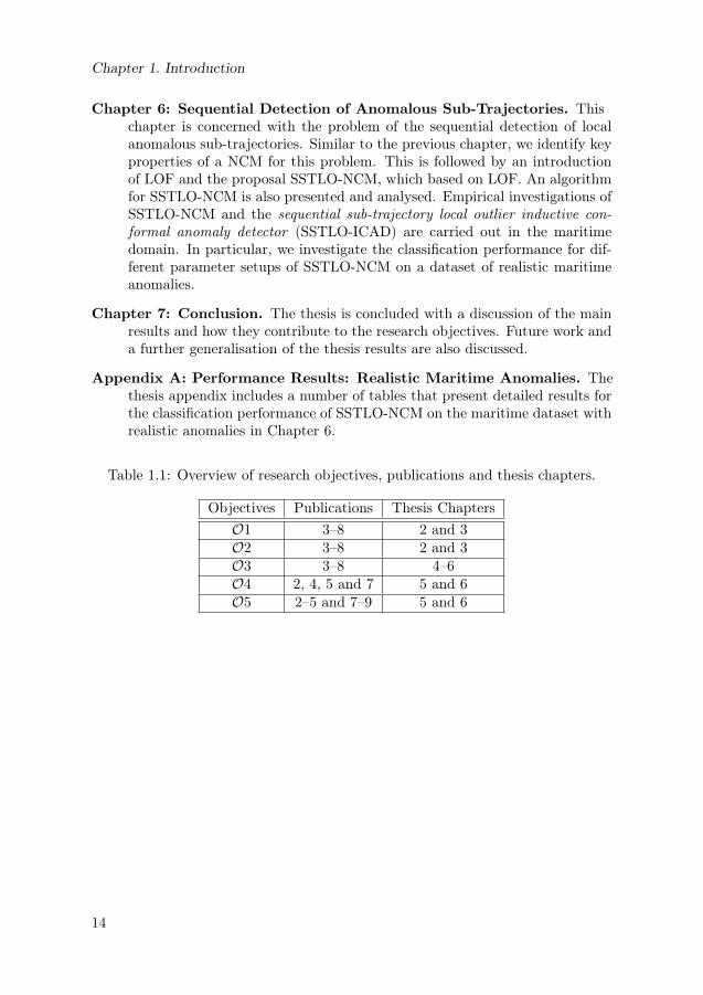
Chapter 6: Sequential Detection of Anomalous Sub-Trajectories. Thischapter is concerned with the problem of the sequential detection of localanomalous sub-trajectories. Similar to the previous chapter, we identify keyproperties of a NCM for this problem. This is followed by an introductionof LOF and the proposal SSTLO-NCM, which based on LOF. An algorithmfor SSTLO-NCM is also presented and analysed. Empirical investigations ofSSTLO-NCM and the sequential sub-trajectory local outlier inductive con-formal anomaly detector (SSTLO-ICAD) are carried out in the maritimedomain. In particular, we investigate the classification performance for dif-ferent parameter setups of SSTLO-NCM on a dataset of realistic maritimeanomalies.
Chapter 7: Conclusion. The thesis is concluded with a discussion of the mainresults and how they contribute to the research objectives. Future work anda further generalisation of the thesis results are also discussed.
Appendix A: Performance Results: Realistic Maritime Anomalies. Thethesis appendix includes a number of tables that present detailed results forthe classification performance of SSTLO-NCM on the maritime dataset withrealistic anomalies in Chapter 6.
Table 1.1: Overview of research objectives, publications and thesis chapters.
Objectives Publications Thesis ChaptersO1 3–8 2 and 3O2 3–8 2 and 3O3 3–8 4–6O4 2, 4, 5 and 7 5 and 6O5 2–5 and 7–9 5 and 6
14

Chapter 2
Background
This chapter presents a background to the subject of the thesis and introduces theterminology and basic concepts required. The first part (Section 2.1) introducesanomaly detection and provides a survey over different aspects of the problem andcommon algorithms. The second part concerns previous work related to anomaloustrajectory detection (Section 2.2).
2.1 Anomaly Detection
Anomaly detection has been identified as an important technique for detectingcritical events in a wide range of data rich domains where a majority of the data isconsidered “normal” and uninteresting (Latecki et al., 2007; Chandola et al., 2009).Yet, it is a rather fuzzy concept and domain experts may have different notions ofwhat constitutes an anomaly (Roy, 2008). Common synonyms to anomaly includeoutlier, novelty, rarity, abnormality, while other related words to anomaly includedeviating, unexpected, suspicious, interesting etc. In the academic world, more orless similar definitions of anomaly detection and the closely related concepts out-lier detection and novelty detection have been proposed by different authors withvarious backgrounds and application areas. However, the methods and algorithmsused in practice are often the same (Chandola et al., 2009).
In the statistical community, the concepts outlier and outlier detection havebeen known for quite a long time. Barnett and Lewis (1994) define an outlier ina dataset to be “an observation (or subset of observations) which appears to beinconsistent with the remainder of that set of data”. A similar definition of anoutlier was given by Hawkins (1980):
[An outlier is] an observation that deviates so much from other ob-servations as to arouse suspicion that it was generated by a differentmechanism.
15

Chapter 2. Background
This mechanism is usually assumed to follow a stationary probability distribution.Hence, outlier detection essentially involves determining whether or not a partic-ular observation has been generated according to the same distribution as the re-maining observations. Traditionally, outlier detection in the statistical communityhas been used to clean datasets before statistical models are fitted; outliers areconsidered noise and are removed to improve the quality of the statistical models.
In the data mining community, “anomalies are patterns in data that do not con-form to a well-defined notion of normal behaviour” (Chandola et al., 2009). Often,the notion of normal behaviour is captured by a normalcy model, which is inducedfrom training data. According to Portnoy et al. (2001), “anomaly detection ap-proaches build models of normal data and then attempts to detect deviations fromthe normal model in observed data”. In contrast to traditional statistical applica-tions, data mining applications are often interested in the anomalous observationsper se, since they may correspond to interesting and important events. Traditionalapplications of anomaly detection in data mining include fraud detection in com-mercial domains (Chandola et al., 2009), intrusion detection in network security(Portnoy et al., 2001), and fault detection in industrial domains (Chandola et al.,2009). Common to all these applications is that patterns of interesting behaviourare difficult, if not impossible, to define a priori, due to limited knowledge andlack of data.
According to Ekman and Holst (2008), “anomaly detection says nothing aboutthe detection approach and it actually says nothing about what to detect”. Indeed,anomaly detection, as it is usually defined, refers to a process that aims to detectsomething ; yet it says nothing in particular about what to detect. This meansthat the interpretation and impact of an anomaly is undefined within the scopeof the anomaly detector. One could argue that the definition of an anomaly isalways relative to a specific model or dataset. Therefore, it is a relative conceptrather than an absolute truth; something that appears to be deviating relative toa statistical model, or strange to a human with limited domain knowledge, may befully understandable and predictable to, e.g., some other model or human domainexpert.
2.1.1 General Aspects of Anomaly Detection
In a recent survey by Chandola et al. (2009), a number of general aspects of theanomaly detection problem are discussed. This section reviews these and otheraspects related to anomaly detection.
Input Data
Similar to other data mining algorithms, most anomaly detection algorithms as-sume that the basic input is in the form of a data point, also referred to as example,data instance, feature vector, observation, object, pattern, etc. The data point canbe univariate or multivariate, but usually has a fixed number of features, also re-ferred to as attributes or variables. These can be a mix of binary, categorical, or
16

2.1. Anomaly Detection
continuous values. However, some methods do not require explicit data points asinput; instead, pairwise distances or similarities between data points are providedin the form of a distance or similarity matrix (Chandola et al., 2009). Anotheraspect of the input is the relationship between different data points, which inmany cases is of a spatial or temporal nature. Trajectory data is an example oftime-series, where data points are temporally ordered. However, most anomalydetection techniques explicitly or implicitly assume that there is no relationshipbetween different data points, i.e., that they are independent of each other (Chan-dola et al., 2009).
Most applications of anomaly detection involve a feature extraction process;this corresponds to preprocessing the raw input data and extracting relevant fea-tures. In the context of moving object surveillance, such features may be currentspeed and location of an object, its size and previously visited locations. Thechoice of an appropriate feature model is critical in anomaly detection applica-tions, since it essentially determines the character of detected anomalies. If, forexample, we only consider the position feature of an object, it will be hard, if notimpossible, to detect anomalies related to the object’s speed, whether it is low orhigh, assuming that speed is more or less independent of position. If inappropriatefeatures are selected, the resulting anomalies may be of little or no interest. Thus,features should be selected carefully and based on available domain knowledge ofhow interesting anomalies manifest themselves.
Output
There are generally two types of output from an anomaly detector; scores andlabels (Chandola et al., 2009). Scoring techniques assign an anomaly or outlierscore to each input data point, where the score value reflects the degree to whichthe corresponding data point is considered anomalous. Output is usually a list ofanomalous data points that are sorted according to their anomaly score. Such alist may include the top-k anomalies, or a variable number of anomalies that havea score above a predefined anomaly threshold. Labelling techniques, on the otherhand, output a label for each input data point, usually normal or anomalous.Such techniques may also output the corresponding anomaly score, confidence orprobability associated with the label. More details regarding the output of differentalgorithms are discussed in Sections 2.1.2 and 2.1.3 below.
Supervised, Unsupervised and Semi-Supervised Anomaly Detection
From an application owners point of view, anomaly detection may be considered asa binary classification problem, where each data point either belongs to a normalclass or an abnormal class. The true class of a data point is typically determined bya domain expert, on the basis of his or her experience of what is normal or uninter-esting, and what is abnormal and therefore interesting. Assuming that a trainingset of data points from both the normal and abnormal class is available, where eachdata point is annotated by a label indicating whether it is normal or abnormal,
17

Chapter 2. Background
supervised learning techniques (Mitchell, 1997) are applicable. In practice, how-ever, the collection and annotation of a labelled training set for supervised learningis typically not feasible, due to the rarity and diversity of abnormal data points.Nevertheless, usually there are large amounts of unlabelled data available, which isassumed to only include a minority, if any, of abnormal data points. Thus, manyanomaly detection algorithms adopt unsupervised learning techniques (Mitchell,1997), such as density estimation or clustering, to find the most anomalous datapoints in a set of unlabelled data. These approaches are referred to as unsupervisedanomaly detection (Chandola et al., 2009). In some cases, normal training datais available, which can be used to learn one-class anomaly detectors or multi-classanomaly detectors, depending on whether the training data includes labelled datapoints from a single normal class or multiple normal classes, respectively (Chan-dola et al., 2009). One-class anomaly detectors, e.g., the one-class Support VectorMachine (SVM) (Schölkopf et al., 1999), classify unlabelled data points as eithernormal or anomalous. Multi-class anomaly detectors can, in addition to this,discriminate data points from different normal classes. Approaches that assumeall training data is labelled normal are sometimes referred to as semi-supervisedanomaly detection (Chandola et al., 2009).
Classification Performance
Assuming that data points belong to either a normal or abnormal class (as dis-cussed above), anomaly detectors are typically evaluated in terms of their classi-fication performance on a labelled evaluation set that includes data points fromboth classes. In particular, the following performance measures from the fieldsof pattern recognition and machine learning are often used to evaluate anomalydetectors:
• Accuracy (Fawcett, 2006), which is equivalent to the overall rate of correctlyclassified data points.
• True positives rate (Fawcett, 2006), also referred to as sensitivity or recall(Fawcett, 2006), which is equivalent to the rate of data points from theabnormal class that are correctly classified as anomalous.
• False positives rate (Fawcett, 2006), also known as false alarm rate (Fawcett,2006), which is equivalent to the rate of data points from the normal classthat are incorrectly classified as anomalous.
• Precision (Fawcett, 2006), which is equivalent to the fraction of the datapoints classified as anomalous that belong to the abnormal class. In otherwords, precision corresponds to the rate of anomaly detections or alarmsthat are interesting from a domain experts perspective.
Obviously, the higher the accuracy, sensitivity and precision, and the lower thefalse alarm rate, the better the performance of the anomaly detector. It shouldbe noted that acquiring a labelled evaluation set may be difficult for the same
18
2.1. Anomaly Detection
reasons that acquiring a labelled training set is difficult (see the discussion aboveregarding supervised anomaly detection).
Types of Anomalies
Chandola et al. (2009) categorise anomalies as either point anomalies, contextualanomalies or collective anomalies. Point anomalies correspond to individual datapoints that are anomalous relative to all other data points; these type of anomaliesare captured by, e.g., the definition of an outlier given by Hawkins (1980). Pointanomalies are the focus of most research within anomaly detection algorithms(Chandola et al., 2009). Contextual anomalies, also known as conditional anom-alies, are data points that are considered anomalous in a particular context. Toformalise the notion of context, each data point is defined by contextual attributesand behavioural attributes (Chandola et al., 2009). If the behavioural attributesof a data point are anomalous relative to the behaviour attributes of the subsetof data points having the same or similar contextual attributes, the correspondingdata point is considered a contextual anomaly. Examples of contextual attributescould be time of day, season and geographical location. Lastly, collective anom-alies consist of a set or sequence of related data points that are anomalous relativeto the rest of the data points. In this case, the individual data points may not beanomalous by themselves; it is the aggregation of the data points that is anom-alous. Examples of collective anomalies can found in sequence data, graph dataand spatial data (Chandola et al., 2009). Anomalous trajectories, which we areconcerned with further on in the thesis, can be considered as instances of collectiveanomalies.
Online vs. Offline Learning
Learning in most anomaly detection algorithms is essentially offline; static modelparameters are learnt from a batch of training data and then used repeatedly whenclassifying new data. In order to accurately model normalcy, a fairly large trainingset may be required, which is representative of all possible normal behaviour.However, such a dataset may not be available from the outset. Moreover, “inmany domains normal behaviour keeps evolving and a current notion of normalbehaviour might not be sufficiently representative in the future” (Chandola et al.,2009). In contrast, online learning may account for this by incrementally refiningand updating model parameters based on new data points.
Algorithms for Anomaly Detection
A number of surveys attempting to structure different algorithms for anomaly de-tection have been published during the last few years (see, e.g., Chandola et al.,2009; Patcha and Park, 2007). Chandola et al. (2009) categorise algorithms asbelonging to one or more of the following classes: classification-based techniques,parametric or non-parametric statistical techniques, nearest neighbour-based tech-niques, clustering-based techniques, spectral techniques and information theoretic
19

Chapter 2. Background
techniques. In their survey, various advantages and disadvantages of algorithmsfrom each category are discussed at length.
2.1.2 Statistical Anomaly Detection
Statistical methods for anomaly detection are based on the assumption that “nor-mal data instances occur in high probability regions of a stochastic model, whileanomalies occur in the low probability regions of the stochastic model” (Chandolaet al., 2009). It is usually assumed that normal data points constitute independentand identically distributed (IID) samples from a stationary probability distribu-tion P , which can be estimated from sample data D. Given a new data point, z,the goal is to determine whether it can be assumed to have been generated by Por not, i.e., if it is anomalous or not relative to the sample data D. Hence, thereare two practical problems: how to estimate P based on D, and how to decidewhether z is a random sample from P .
Parametric Methods and GMM
Statistical methods for estimating probability distributions can broadly be categor-ised as either parametric or non-parametric models (Markou and Singh, 2003a).Starting with the parametric models, they assume that the underlying distribu-tion belongs to a parameterised family of distributions, i.e., Pθ : θ ∈ Θ, where theparameters θ belong to a parameter space Θ and can be estimated from availablesample data D. A common and simple parameterised model in anomaly detectionapplications is theGaussian distribution (Chandola et al., 2009; Markou and Singh,2003a). Another example is the Poisson distribution (Holst et al., 2006). Morecomplex parameterised models in anomaly detection applications include variousgraphical models, such as Bayesian networks (Johansson and Falkman, 2007) andhidden Markov models (HMM) (Urban et al., 2010), and mixture models, suchas the univariate or multivariate Gaussian mixture model (GMM) (Laxhammar,2008; Ekman and Holst, 2008) and mixtures of other parameterised distributions,such as the Poisson and Gamma distributions (Ekman and Holst, 2008).
GMM is a common model for approximating continuous multi-modal distri-butions, when knowledge regarding the structure is limited; it has been used innumerous anomaly detection applications (Chandola et al., 2009). A GMM con-sists of C multivariate Gaussian densities known as mixture components. EachGaussian component ci, i = 1, . . . , C, has its own parameter values θi = (µi,Σi)and weight wi, where µi is the mean value vector, Σi is the covariance matrix andwi is a non-negative normalised mixing weight where all weights sum to one. Thetotal set of parameters for the GMM is denoted θ = {θ1, . . . , θC , w1, . . . , wC}. Theprobability density function for the multivariate GMM is given by:
p (x) =
C∑i=1
wi1
(2π)d/2√|Σi|
exp
(−1
2(x− µi)>Σ−1
i (x− µi)). (2.1)
20

2.1. Anomaly Detection
A common and relatively simple way to estimate the parameters θ of a dis-tribution Pθ based on a data sample D is to use a maximum likelihood (ML)estimator. The expectation-maximisation (EM) algorithm (Dempster et al., 1977)is a widely used ML estimator when D is incomplete and data points may havemissing values, also known as latent variables. One example of missing values isnot knowing which of the components of a mixture model that generated a datapoint. Typically, the EM algorithm starts by randomising initial values for theparameters and then incrementally estimating the values θ̂ that yield maximumlikelihood for the sample data D:
θ̂ = argmaxθ∈Θ
(D|θ) . (2.2)
More specifically, the algorithm consists of two steps, expectation and maximisa-tion, which are repeated until a certain end condition, usually a convergence condi-tion, is fulfilled. In the case of a GMM with a predefined number of components C,the expectation step involves updating the posterior probabilities p (ci |xj ) for eachdata point xj ∈ D, j = 1, . . . . , n, belonging to each component ci, i = 1, . . . , C,according to Bayes’ rule (Verbeek, 2003):
p (ci |xj ) =p (xj ; ci)wi∑
q=1,...,C
p (xj ; cq)wq, (2.3)
where
p (xj ; cq) =1
(2π)d/2√|Σq| exp
(−1
2(xj − µq)>Σ−1
q (xj − µq))
(2.4)
corresponds to the qth component distribution. This expectation of point to com-ponent correspondence is then used in the maximisation step where the parametersof each component are updated based on the ML estimation. The maximisationstep involves adjusting the parameters of each component in such a way that thecomponent better fits the data points, taking the updated posterior probabilitiesinto account. More specifically, component parameters are updated according toEquations 2.5 to 2.7 (Verbeek, 2003):
wi =1
n
n∑j=1
p (ci |xj ) , (2.5)
µi =1
nwi
n∑j=1
p (ci |xj )xj , (2.6)
Σi =1
nwi
n∑j=1
p (ci |xj ) (xj − µi) (xj − µi)> . (2.7)
The updated model is then used to calculate new posterior probabilities in theexpectation step, and so on.
21

Chapter 2. Background
The popularity of the standard EM algorithm is probably due to its relativesimplicity and fast convergence. Nevertheless, it has some disadvantages: Firstly,it is not guaranteed to converge to a global optimum; the algorithm is more orless sensitive to the parameter initialisation and may converge to different MLestimates depending on the start values (Verbeek, 2003). The standard procedureto overcome this initialisation dependence is to start the EM algorithm from sev-eral random initialisations and to retain the best result obtained (Verbeek, 2003).An extension of the standard EM algorithm calculates the maximum a posteriori(MAP) estimate based on a prior distribution, p (θ), on the parameters, thus incor-porating prior knowledge and making the algorithm less sensitive to initialisationand noisy data. Another issue is how to determine the optimal number of com-ponents, a problem which is not solved by the standard EM algorithm. Verbeekproposed an efficient and greedy version of the EM algorithm that estimates theoptimal number of components of a GMM and avoids the need for multiple runswith random parameter initialisation (Verbeek et al., 2003).
ML and MAP estimators do not include any uncertainty in the parameter es-timates; they simply calculate the most likely parameter values for a given dataset,regardless of the size of the dataset. Hence there is no information on how confid-ent we can be in the estimates. In the case of a small sample, the estimates aresusceptible to random variations in the data; this is a bad property for an anomalydetector, since it will generate a lot of false alarms by focusing on the peculiaritiesof the data too much (Holst et al., 2006). Moreover, in many applications, in-cluding anomaly detection, we are not interested in the model’s parameter valuesper se; rather, we are interested in getting an accurate and reliable estimate ofthe predictive data distribution, p (x), based on the sample data D. In this case,an alternative to ML or MAP is a fully Bayesian parameter estimation, wherethe posterior distribution for the parameter values, p (θ|D), is estimated based onthe prior distribution, p (θ), and available sample data, D, according to Bayes’theorem (Gelman et al., 2003):
p (θ|D) =p (D|θ) p (θ)´
θp (D|θ) p (θ) dθ
. (2.8)
The posterior distribution for the parameters can then be used to estimate thepredictive distribution for normal data (Holst et al., 2006):
p (x|D) =
ˆθ
p (x|θ) p (θ|D) dθ. (2.9)
Non-Parametric Methods and KDE
A general drawback of the parametric techniques is their assumption that a para-meterised model exists and that it can be accurately estimated; this is doubtful inmany applications where the true structure of the probability distribution is un-known and may be highly complex (Markou and Singh, 2003a). One approach tomitigate this problem is to resort to non-parametric methods, such as histograms
22

2.1. Anomaly Detection
or kernel density estimators (KDE), which essentially assume nothing about thestructural form of the distribution; it is instead determined from the given data(Chandola et al., 2009; Markou and Singh, 2003a).
In histogram-based methods, the feature space is assumed to be discrete andeach possible value corresponds to a bin of the histogram. The histogram is con-structed by simply counting the number of data points that fall within each ofthe bins. The unknown data distribution is then approximated by the discretedistribution of observed data points from the different bins, i.e., the relative fre-quency. A drawback of histogram methods is that continuous input data has tobe discretised. It may not be obvious how the discretisation should be done, andsubtle, yet significant, information may be lost in the process. Determining theoptimal size of the bins is a key challenge for maintaining a low false alarm (falsepositive) rate and low false negative rate in anomaly detection applications (Chan-dola et al., 2009). Histogram methods for anomaly detection in multivariate datatypically construct a separate univariate histogram for each data feature (Chan-dola et al., 2009). Thus, they do not capture the potential correlation betweendifferent features. However, there is at least one exception to this, in which thecorrelation between different attributes is accounted for by considering a variantof a multi-dimensional histogram (Brax et al., 2008).
In contrast, KDE, also known as Parzen window estimation, allows for a non-parametric estimation of a multivariate continuous distribution based on a kernelfunction (Chandola et al., 2009). The unknown distribution is approximated byplacing a kernel function K on each and every data point xi of the data sample:
p (x) =1
n
n∑i=1
1
(hi)dK
(x− xihi
), (2.10)
where n is the size of the sample data, d is the number of dimensions of the datapoints and hi is a kernel width parameter known as bandwidth (Latecki et al.,2007), window width (Ristic et al., 2008) or smoothing parameter (Markou andSingh, 2003a). The kernel function is usually a symmetric probability densityfunction, being non-negative over its domain and should integrate to unity overthe defined range (Markou and Singh, 2003a). A common kernel for anomalydetection applications is the multivariate Gaussian function with zero mean andcovariance matrix Σ (Ristic et al., 2008; Latecki et al., 2007):
K (x) =1
(2π)d/2√|Σ|
exp
(−1
2x>Σ−1x
). (2.11)
The covariance matrix Σ can be set to, e.g., the identity matrix (Latecki et al.,2007) or estimated from data as sample covariance (Ristic et al., 2008). The kernelwidth can either be fixed, i.e., the same for all data points, or adaptive, based onthe local (Latecki et al., 2007) or global (Ristic et al., 2008) distribution of thedata points. A formula for computing the optimal fixed width for the Gaussiankernel (under the assumption that the underlying PDF is Gaussian) was originallyproposed by Silverman (1986). However, a fixed kernel width is inappropriate in
23

Chapter 2. Background
applications where local data density varies (Latecki et al., 2007). In particular,a fixed kernel width is unable to satisfactorily deal with the tails of distributionswhere local density is low (Ristic et al., 2008). Therefore, kernel widths shouldbe adaptive based on the local data density, i.e., broader windows in low densityareas and narrower windows in high density areas. A two-stage approach, knownas adaptive KDE for computing adaptive window widths from the fixed optimalwidth, was proposed by Silverman (1986). Another approach where local windowwidths are based on distance to the kth nearest neighbour was presented by Lateckiet al. (2007). There are, however, at least two general drawbacks with KDEmethods: they are relatively sensitive to noise in data (Markou and Singh, 2003a)and they require a relatively large sample set for accurate density estimation.
Anomaly Detection in New Data
Assuming that P has been estimated based on a parametric or non-parametricmethod, as discussed above, various anomaly tests for a new data point z have beenproposed (Chandola et al., 2009). Some of these compute an anomaly score, whichdepends on the probability (discrete data) or probability density value (continuousdata), and classify the data point as anomalous if the score is above a particularthreshold. Often, the anomaly score is simply the inverse or negative of the datalikelihood or its logarithm. Other approaches are based on statistical hypothesistesting where the null hypothesis, H0, that z constitutes a random sample fromthe estimated distribution p (x) is tested (Chandola et al., 2009). These tests arebased on a specified test statistic and significance level, which corresponds to theconfidence in classifying a data point as anomalous.
For Gaussian models, such as the simple Gaussian distribution or mixtures ofGaussian distributions, a large number of anomaly measures and test statisticsfor classifying new data points as normal or anomalous have been proposed. Asimple technique is to calculate the number of standard deviations σ from thecorresponding mean µ and compare this distance to a threshold (Markou andSingh, 2003a). For example, in one dimension, data points located 3σ or morefurther away more from µ may be classified as anomalous, as the region µ ± 3σcontains 99.7% of all data points from the corresponding distribution (Chandolaet al., 2009). A similar anomaly measure for univariate or multivariate data is thebox plot rule, which usually defines a region that contains 99.3% of the normaldata points (Chandola et al., 2009). A well-known outlier test is Grubb’s test,where the z-score for a univariate data point is calculated and compared to anadaptive threshold based on data size and the value of a t-distribution taken at aspecified significance level (Chandola et al., 2009). Multiple variants of Grubb’stest have been proposed for multivariate data (Chandola et al., 2009). A numberof other test statistics for anomaly detection have also been proposed for univariateand multivariate data, including Student’s t-test, Hotelling’s t2-test and χ2-tests.Common to all these test statistics is the assumption that the underlying datadistribution is Gaussian.
Ekman and Holst (2008) proposed principal anomaly as “the true anomaly
24

2.1. Anomaly Detection
measure”. Assuming that X is a random variable from the probability distributionp (x), the principal anomaly of a data point z with respect to p (x) is defined asPr {p (X) ≥ p (z)}, i.e., the probability that a random sample X has a densityequal to or larger than the density of z (Ekman and Holst, 2008). This measureis attractive from a theoretical perspective, since it is normalised and does notassume that p (x) is Gaussian. However, it is typically not easy to estimate theprincipal anomaly for multivariate distributions and distributions other than theGaussian (Ekman and Holst, 2008). Therefore, Ekman and Holst (2008) proposeddeviation as an alternative anomaly measure, which is defined as:
E [log p (X)]− log p (z)
S [log p (X)], (2.12)
where E and S correspond to the expectation (mean) and standard deviation,respectively. They argue that this measure is strongly related to principal anom-aly and show how it can be easily calculated for multivariate distributions withindependent variables (Ekman and Holst, 2008).
In histograms-based methods, there are generally two approaches to anomalydetection. The first is to simply check whether a new data point falls into any one ofthe histogram bins; if it does, the data point is classified as normal, otherwise, it isanomalous (Chandola et al., 2009). The second approach assigns an anomaly scoreto each data point, based on the frequency of the corresponding bin (Chandolaet al., 2009). If frequency is below a specified threshold, the data point is classifiedas anomalous.
For other non-Gaussian distributions, such as Bayesian networks, HMM, KDE,etc., anomaly detection is usually done by checking whether the likelihood p (z),or the corresponding logarithmic likelihood, log (p (z)), for the new data pointis below an application specific anomaly threshold. A low likelihood indicatesan improbable data point and, hence, evidence against the hypothesis that itis normal. More generally, a higher anomaly likelihood threshold increases theprobability of detecting true anomalies, but also the probability of false alarms.
2.1.3 Other Anomaly Detection Algorithms
Classification-Based Methods
Classification-based methods essentially assume that a decision boundary in fea-ture space can be learnt from a training dataset, such that the decision boundaryseparates normal and anomalous data points. Depending on the number of nor-mal classes, classification-based anomaly detectors can be grouped into one-class ormulti-class anomaly detectors. Multi-class anomaly detectors assume that trainingdata includes labels from multiple normal classes. Typically, new data points areeither classified as belonging to one of the normal classes, or classified as anom-alous, if they do not fit any of the normal classes. One-class techniques assumethat all data points in the training set have the same label; they typically learn a
25

Chapter 2. Background
discriminative boundary around the training data which is used to check whethernew data points are anomalous or not.
Most of the classification-based methods for anomaly detection are based onneural networks, support vector machines (SVM) or rule-based methods (Chan-dola et al., 2009). Considering neural networks, multi-layer perceptrons are thebest-known and most widely used (Markou and Singh, 2003b). Other neuralnetworks used for anomaly detection include auto-associative networks, adaptiveresonance theory, radial basis functions and Hopfield networks (Chandola et al.,2009). Neural networks are powerful classifiers, since they can approximate arbit-rary complex decision boundaries in feature space. However, they are designed fordiscriminating between multiple known classes rather than detecting new classes(Markou and Singh, 2003b). Since they do not generate closed class boundaries,adapting them to anomaly (novelty) detection and ensuring that the generalisa-tion property of the network does not interfere with its anomaly detection abilityare fairly challenging tasks (Markou and Singh, 2003b). In other words, there istypically the risk of overfitting the model to the training data.
A number of different SVM-based methods have been applied to anomaly de-tection in the one-class setting (Chandola et al., 2009). Similar to neural networks,SVM methods are capable of learning arbitrary complex regions in input featurespace. However, they do not have the same problem of overfitting to training data,since they estimate optimal wide-margin hyperplanes in a high-dimensional fea-ture space. A key parameter of any SVM is the kernel function, e.g., a polynomialor Gaussian function, which maps input data to a high-dimensional feature spacewhere data is perfectly, or close to, linearly separable. Schölkopf et al. (1999) pro-posed a one-class SVM for novelty detection based on quantile estimation of arbit-rary distributions. The idea is to learn the boundaries in input data feature spacefor a specified quantile of the underlying distribution, based on available trainingdata. For example, estimating the boundaries for the first percentile results ina region containing approximately 99% of randomly generated data points fromthe underlying distribution. The specified quantile corresponds to the anomalythreshold; if a new data point falls outside of the region, it is considered anom-alous. The region is found by estimating the hyperplane in the high-dimensionalfeature space that maximises the distance to the origin where only a small fractionof the training data points fall between the hyperplane and the origin (Schölkopfet al., 1999).
Various methods that learn rules from normal data based on, e.g., decisiontrees, have been proposed for anomaly detection (Chandola et al., 2009). Someof these methods associate a confidence score to each rule, which is proportionalto the ratio of the number of training instances correctly classified by the ruleand the total number of training data points covered by the rule (Chandola et al.,2009). For new data points, the rule that best captures the data points is sought,and the inverse of the corresponding rule confidence is returned as the anomalyscore. If no rule that captures the new data point can be found, it is classified asanomalous.
26

2.1. Anomaly Detection
Nearest Neighbours Methods
Nearest neighbours methods for anomaly detection are based on the assumptionthat “normal data [points] occur in dense neighbourhoods, while anomalies occurfar from their closest neighbours” (Chandola et al., 2009). This assumption sug-gests that a distance or similarity measure between data points is needed. For con-tinuous features, the Euclidean distance (ED) is a popular distance measure, butother measures have also been proposed (Chandola et al., 2009). For categoricalattributes, the simple matching coefficient, or other more complex measures, areoften used (Chandola et al., 2009). Generally, distance measures used in nearestneighbours methods are required to be positive-definite and symmetric; but theyare usually not required to satisfy the triangle inequality and, hence, not requiredto be strictly metric (Chandola et al., 2009).
A number of different algorithms for calculating anomaly scores based on thenearest neighbours principle have been proposed. A common algorithm is basedon the following principle: “The anomaly score of a data [point] is defined as itsdistance to its kth nearest neighbour in a given dataset” (Chandola et al., 2009).Other variants of this principle calculate the anomaly score as the sum of thedistances to the k nearest neighbours (Eskin et al., 2002), or as the inverse ofthe number of nearest neighbours that are no more than d distance apart fromthe corresponding data point (Chandola et al., 2009). The latter algorithm hasthe flavour of kernel density estimation (Section 2.1.2) where the kernel functioncorresponds to counting the number of neighbouring data points within the hy-persphere of radius d. However, analogously to statistical methods, the nearestneighbours techniques discussed above may be suboptimal if the data has regionsof varying densities (Chandola et al., 2009). To handle this, techniques for com-puting the local density of data points, i.e., the density of data points relative totheir closest neighbours, have been proposed. One such technique is local outlierfactor (LOF) (Breunig et al., 2000), in which the anomaly score for a particulardata point is equal to the ratio of the average local density of the k nearest neigh-bours, and the local density of the data point itself. The local densities in LOFare inversely proportional to the radius of the minimum hypersphere that con-tains the k nearest neighbours. Several variants and extensions of the basic LOFalgorithm have been proposed, e.g., to handle different data types and improvecomputational efficiency.
In most cases, a threshold is applied to the anomaly score during anomalydetection. Alternatively, the n data points with the largest anomaly scores maybe returned (Chandola et al., 2009).
Clustering Methods
Clustering is essentially an unsupervised learning technique that groups similardata points into clusters. Chandola et al. (2009) categorise clustering based tech-niques for anomaly detection into three groups, depending on what assumptionsare made regarding normal and anomalous data. The first group assumes that
27

Chapter 2. Background
“normal data [points] belong to a cluster in the data, while anomalies do not be-long to any cluster”. These techniques are based on an algorithm that clustersthe data while not forcing all data points to belong to a cluster; data points thatare found not belonging to any cluster are classified as anomalous. According toChandola et al. (2009), the disadvantage of these methods is that they are designedto find clusters rather than anomalies.
The second group of clustering techniques are more focused on finding an-omalies; these are based on the assumption that “normal data [points] lie closeto their closest cluster centroid, while anomalies are far away from their closestcluster centroid” (Chandola et al., 2009). Typically, these methods first cluster thedata and then assign an anomaly score to each data point, based on the distanceto its nearest cluster centroid. Common clustering algorithms include k-meansclustering, self-organising maps (SOM), and EM (Chandola et al., 2009). In EM,clusters are represented as Gaussian components in a mixture model, i.e., similarto the estimation of a GMM (Section 2.1.2). Techniques from the second groupcan also operate in a semi-supervised mode, where new test data is compared toa cluster model learnt from previous training data (Chandola et al., 2009).
If anomalies form clusters by themselves, algorithms based on the two principlespresented above will obviously not be able to detect those anomalies. To addressthis issue, algorithms have been proposed that rely on the assumption that “normaldata [points] belong to large and dense clusters, while anomalies either belongto small or sparse clusters” (Chandola et al., 2009). These algorithms assignan anomaly score which reflects the size or density of the cluster to which thecorresponding data points belong.
2.2 Anomalous Trajectory Detection
Research related to the automated detection of anomalous trajectories has attrac-ted a lot of attention lately, much due to the increasing amounts of historical andreal-time trajectory data. There is a clear trend towards more and more advancedsensor systems producing huge amounts of trajectory data from moving objects,such as people, vehicles, vessels and animals. For example, the use of video cam-eras for public surveillance has increased dramatically since the beginning of the21th century and a significant amount of research has focused on developing objecttracking algorithms (Yilmaz et al., 2006) that produce trajectories from raw videodata. In the maritime surveillance domain, regulations regarding the mandatoryuse of AIS transponders for vessels of 300 gross tonnage or greater have resultedin a significant increase of vessel tracking data, which complements existing radartracking systems (Chang, 2004). In the domain of intelligent transportation, thewidespread use of GPS has facilitated the tracking of land-based transports.
Technically, a trajectory is generally modelled as a finite sequence of datapoints:
(χ1, t1) , . . . , (χL, tL) : ti−1 < ti, i = 2, . . . , L, (2.13)
28

2.2. Anomalous Trajectory Detection
where each χi ∈ Rd is a multi-dimensional feature vector at time point ti and wherethe total length in time of the trajectory is tL − t1 (Morris and Trivedi, 2008a).In the simple case, χi ∈ R2 represents an object’s (estimated) location in thetwo-dimensional spatial plane at time point ti. Depending on the application, thefeature space may be extended by, e.g., a third spatial dimension or the velocity.Moreover, in some applications it is assumed that the trajectory is uniformlysampled in time:
(ti+1 − ti) = (ti − ti−1) : i = 2, . . . , L− 1, (2.14)
in which case (2.13) can be further simplified to:
(χ1, . . . , χL) . (2.15)
It should be noted that in practice, (2.13) is typically the output of a trackingsystem and constitutes an estimate of the true trajectory of the object. Therefore,(2.13) may be inaccurate or incomplete due to various errors and noise introducedby the tracking system. In particular, the trajectory may appear anomalous dueto erroneous measurements and other noise.
Most of the previous work related to anomalous trajectory detection has beenpublished in the domains of video surveillance and maritime surveillance. In thefollowing two subsections, we therefore provide a survey of previous algorithmswithin each of these two domains.
2.2.1 Video Surveillance
A large amount of work related to the automated detection of anomalous traject-ories has been published in the domain of video and image processing (Morris andTrivedi, 2008a; Hu et al., 2006; Dee and Velastin, 2008). Most of these methodsinvolve trajectory clustering, where cluster models corresponding to normal pathsor routes are learnt from historical trajectories; this process is referred to as tra-jectory learning (Morris and Trivedi, 2008a) and is presented in the first part ofthis subsection. New trajectories are typically assigned an anomaly score based onthe distance to the closest cluster model, or likelihood of the most probable clustermodel; this is described in the second part of this subsection. Finally, methodsthat do not involve trajectory clustering are presented in the third and final partof this subsection.
Trajectory Learning
Trajectory learning typically consists of three steps that are sometimes combined:preprocessing of raw trajectories, clustering of preprocessed trajectories and mod-elling of trajectory clusters (Morris and Trivedi, 2008a).
The purpose of the preprocessing is to produce trajectory representations thatare suitable for clustering. A typical problem with raw trajectories is that theyare not of equal length. According to Morris and Trivedi (2008a), “steps must
29

Chapter 2. Background
be taken to ensure a meaningful comparison between differing sized inputs” and“trajectory representations should retain the intuitive notion of similarity presentin raw trajectories for meaningful clusters”. Two main techniques are used for pre-processing trajectories: normalisation and dimensionality reduction (Morris andTrivedi, 2008a). Normalisation techniques ensure that trajectories are of equallength by, e.g., extending short trajectories by zero padding (Hu et al., 2006) orby re-sampling trajectories. Dimensionality reduction techniques map trajectoriesinto a lower dimensional feature space which is computationally more manageableand enables more robust clustering given less training data (Morris and Trivedi,2008a). Examples of dimensionality reduction techniques include vector quantisa-tion, various polynomial approximations (Naftel and Khalid, 2006), parametrisedspline models (Sillito and Fisher, 2008), wavelets, HMM (Porikli, 2004), principalcomponent analysis (PCA), and spectral methods (Atev et al., 2010).
The aim of the trajectory clustering is to learn the underlying structure androutes in data by grouping similar trajectories. All clustering algorithms requirethat an appropriate similarity measure, also known as distance measure, is defined.Assuming that all the points of each trajectory are embedded as a high-dimensionalvector, the ED (Euclidean distance) between two such vectors is perhaps the mostsimple and intuitive similarity measure. However, ED requires that the prepro-cessed trajectories are of equal length, and it performs poorly if the trajectoriesare not properly aligned (Morris and Trivedi, 2008a). Other similarity measuresand modifications of ED have been proposed for relaxing alignment and lengthconstraints, such as dynamic time warping (DTW) (Morris and Trivedi, 2008a).Longest common sub-sequence (LCSS) is another similarity measure appropriatefor trajectories that are of unequal length and/or are not well-aligned (Vlachoset al., 2002). In contrast to ED and DTW, LCSS is more robust to noise in tra-jectories, since it focuses on parts of the trajectories that are similar rather thandissimilar (Vlachos et al., 2002). Other alternatives to ED include HMM-basedtrajectory distance (Porikli, 2004) and variants of the Hausdorff distance (HD)(Atev et al., 2010) (HD is described in Section 5.1.1). Different similarity meas-ures, including those presented above, were evaluated for trajectory clustering ona real-world dataset by Zhang et al. (2006). They found that a relatively simpleapproach based on representing trajectories in a PCA-based coefficient featurespace and using ED as distance measure performed the best.
A number of different algorithms have been proposed for creating and updat-ing trajectory clusters based on a specified similarity measure. Morris and Trivedi(2008a) identified five main categories based on fundamental properties of theclustering algorithm: iterative optimisation (e.g., k-means), online adaptive, hier-archical methods (agglomerate and divisive), neural networks (e.g., SOM) and co-occurrence methods. The strengths and weaknesses of each category are discussedin their survey (Morris and Trivedi, 2008a). Of particular interest are clusteringalgorithms that are online adaptive, since they enable the continuous and efficientupdate and adaption to changes in normal trajectory behaviour. Piciarelli andForesti (2006) proposed such an algorithm for online clustering of trajectories,
30

2.2. Anomalous Trajectory Detection
including a novel similarity measure tailored for the clustering algorithm.Once trajectories have been clustered, appropriate cluster models, sometimes
referred to as path models (Morris and Trivedi, 2008a) or motion patterns (Huet al., 2006), are defined. The path models correspond to compact representationsof the clusters, which enables efficient inference during, e.g., trajectory classific-ation or anomaly detection. Two main types of path models have been adopted.The first considers a complete path, from starting point to endpoint. The seconddecomposes a path into smaller atomic parts called subpaths (Morris and Trivedi,2008a). Complete path models are typically based on a centroid representation ofthe cluster, corresponding to the “average” trajectory (Morris and Trivedi, 2008a).The centroid is sometimes complemented by an envelope, which captures the exten-sion and variance of the trajectories (Morris and Trivedi, 2008a). Hu et al. (2006)represent each path model (referred to as motion pattern) as a chain of Gaussiandistributions, where the sequence of mean values and covariance matrices definethe centroid and envelope, respectively. Morris and Trivedi (2008b) proposed themodelling of each path by a HMM where each hidden state is modelled by a GMM.Model parameters for each HMM are initially estimated based on the training tra-jectories belonging to the corresponding cluster. Each HMM can also be updatedonline as new training data arrives. In the case of subpath models, these are fur-ther defined by their connections to other subpaths, which can be probabilisticallymodelled (Morris and Trivedi, 2008a). An example of a subpath structure wasproposed by Piciarelli and Foresti (2006), where each subpath is modelled as anode in a tree-like structure augmented with probabilities for node transitions. Asubpath in their approach is represented as a sequence of points, where each pointhas an associated variance, i.e., similar to Hu et al. (2006).
Anomaly Detection
For complete trajectories, anomaly detection is typically carried out by first de-termining the path model that best explains the new trajectory, i.e., having theminimal distance to the new trajectory. In the case of probabilistic models, thiscan be done on the basis of a MAP or ML analysis (Morris and Trivedi, 2008a).The corresponding distance or likelihood is then usually compared to an anom-aly threshold, analogously to general anomaly detection algorithms discussed inSection 2.1. Some algorithms, but far from all, support sequential, also knownas online (Morris and Trivedi, 2008a) or incremental (Hu et al., 2006) anomalydetection in incomplete trajectories. Morris and Trivedi (2008b) proposed an al-gorithm that monitors the likelihood for the part of the current trajectory that iswithin a sliding window of a fixed size; if this likelihood drops below a specifiedthreshold, the trajectory is classified as anomalous. Hu et al. (2006) proposed analgorithm for incremental anomaly detection in incomplete trajectories; for eachnew data point, the algorithm first updates the most probable motion pattern(trajectory cluster model) given the part of the trajectory observed so far. Thelikelihood for the new point is then calculated relative to the most probable mo-tion pattern and the point is classified as anomalous if its likelihood is below a
31

Chapter 2. Background
specified threshold. If a series of points are classified as anomalous, the trajectoryis classified as anomalous. Fu et al. (2005) proposed a sequential anomaly detec-tion algorithm that incrementally determines the MAP trajectory cluster as moredata points are observed for an incomplete trajectory. The incomplete trajectoryis classified as anomalous if it leaves the envelope of the current MAP cluster,the MAP cluster varies as more data points are observed, or the velocity of thetrajectory deviates from the corresponding velocity of the current MAP cluster.
Non-clustering Based Methods
Other approaches to trajectory anomaly detection in video surveillance have beenproposed that do not involve the clustering of trajectories as presented above (Pi-ciarelli et al., 2008; Yankov et al., 2008; Brax et al., 2008; Owens and Hunter,2000). Piciarelli et al. (2008) proposed a trajectory learning and anomaly detec-tion algorithm based on one-class SVM (Section 2.1.3), where each trajectory isrepresented by a fixed-dimensional feature vector corresponding to evenly sampledpoints from the raw trajectory. One of the main novelties of the algorithm is itsability to automatically detect and remove anomalies in the training data.
Yankov et al. (2008) proposed the application of time-series discords (Keoghet al., 2005) for detecting anomalous trajectories in a database. Assuming pre-processed trajectories or sub-trajectories of equal length, a discord is defined asthe trajectory or sub-trajectory, respectively, maximising the ED to its nearestneighbour in the database. This definition can be extended by considering thedistance to the kth nearest neighbour. Moreover, if the dataset is assumed to in-clude more than one anomalous trajectory, anomaly detection can be carried outby calculating the top-K discords.
Brax et al. (2008, 2009) proposed an algorithm based on multi-dimensionalhistograms for detecting anomalous trajectory behaviour in video surveillance.Each data point from a trajectory is represented in a discrete multi-dimensionalfeature space, referred to as a composite state space, which encompasses: currentkinematic state (position, speed and course), the object’s position relative to thecurrently closest other object, the object’s size, the state of the local environment,and the time of the day. A multi-dimensional histogram is constructed for thecomposite states of all the data points in the training set. Moreover, a separatehistogram for each possible transition from a composite state to another is alsoconstructed. Sequential anomaly detection is based on the relative frequency ofeach new data point according to the histograms. If the average frequency of themost recent data points within a sliding window is below a predefined threshold,the trajectory is classified as anomalous. One of the main features of this approachis that contextual information, i.e., time of day and state of local environment,is embedded in the state (feature) space. Moreover, the proposed method differsfrom traditional multi-histograms in that the state boundaries are set on the basisof expert knowledge rather than generated from the data itself (Brax et al., 2009).
Owens and Hunter (2000) proposed an algorithm based on SOM appropriatefor learning and sequential (online) anomaly detection in trajectory data. Each
32

2.2. Anomalous Trajectory Detection
data point from a trajectory is represented by a fixed-length feature vector encom-passing the current location, velocity, and acceleration, together with informationon the recent position. The SOM is trained using a set of feature vectors as in-put. During sequential anomaly detection, the feature vector corresponding toeach new data point is submitted to the SOM and the ED to the winning neuronis determined. If this distance exceeds a predefined threshold, the correspondingtrajectory is classified as anomalous.
Lee et al. (2008) proposed a partition-and-detect framework for the detection ofanomalous sub-trajectories in a trajectory database. A proposed two-step anomaly(outlier) detection algorithm first partitions each trajectory into a number of linesegments. Next, anomalous trajectory partitions, i.e., line segments, are detectedaccording to a combination of distance-based and density-based analysis. In thecase of distance, a combination of spatial distance and angular distance betweenline segments is used.
2.2.2 Maritime Surveillance
Maritime surveillance is another domain for which substantial work related toanomaly detection in trajectory data has been published. In contrast to videosurveillance, most of the algorithms proposed for anomaly detection in the mari-time domain do not involve the explicit clustering of trajectories as part of thelearning phase. The published papers typically provide less information on para-meter values and implementation details of the proposed algorithms. Moreover,the experiments are often described in less detail and the datasets are exclus-ively non-public. Hence, it is generally more difficult to actually implement theproposed algorithms and reproduce the experiments.
A number of methods have been proposed where learning is based on theestimation of a statistical model for the feature values of individual data pointsfrom vessel trajectories, e.g., the current location and velocity vector (Brax et al.,2010; Johansson and Falkman, 2007; Ristic et al., 2008; Kraiman et al., 2002). Inthe work by Ristic et al. (2008), vessel trajectories are first clustered on the basisof their origin, resulting in a number of motion patterns. The PDF for featurevalues of data points belonging to the same motion pattern is then estimated usingKDE. Data points from new trajectories are sequentially classified as normal oranomalous on the basis of their likelihood, which is calculated from the PDF of thecorresponding motion pattern. Kraiman et al. (2002) discuss a two-step learningalgorithm where feature values of individual data points are first clustered usingSOM and then modelled using GMM. Anomaly detection in new data is carriedout on the basis of a Bayesian analysis of the probability output of the GMM,which can be accumulated within a sliding time window. A prototypical scenariois presented where properties of the proposed algorithm are discussed. However,no details regarding the learning and anomaly detection algorithm are given.
Other statistical approaches have also been proposed based on Bayesian net-works (Johansson and Falkman, 2007) or multi-dimensional histograms (Braxet al., 2010), where point features are discretisized and anomaly scores for new
33

Chapter 2. Background
data points are calculated on the basis of their likelihood or frequency in trainingdata, respectively. Johansson and Falkman (2007) argue that one of the mainadvantages of the Bayesian network is that it enables the incorporation of humanexpert knowledge during learning. The multi-histogram method proposed by Braxet al. (2010) has the advantage that it, in contrast to the previous algorithms, cap-tures the relationship between successive data points by modelling the frequency ofdifferent state transitions. In order to suppress the effect of noise during anomalydetection, Johansson and Falkman (2007) and Brax et al. (2010) propose a slidingwindow approach where anomaly scores for individual data points are integrated,i.e., similar to Kraiman et al. (2002) described above.
Urban et al. (2010) propose a two-level approach based on a combination ofGMM and HMM for learning and anomaly detection in trajectory data. At the firstlevel, a GMM is estimated for the position feature of individual trajectory pointsbased on EM. At the second level, each component of the GMM is considereda discrete state in a HMM, which is estimated from the trajectory data usingthe Baum-Welch algorithm. Anomaly detection in new trajectories is carried outby thresholding the likelihood according to the HMM. Classification performanceof the algorithm is evaluated on a non-public simulated dataset. A similar two-level approach was proposed by Tun et al. (2007), in which clusters, referred to asregions, in the position feature space for vessel trajectories are first discovered usinga combination of density maps and Linear scale space. A HMM is then estimatedfor the transitions between different regions. Moreover, additional feature values,such as momentary course and speed, are estimated for vessel trajectories withinthe same region. A short extract from an experimental evaluation with real normaldata and simulated anomalous data show that the method can accurately detectthe anomalies.
Rhodes et al. (2005, 2007), Garagic et al. (2009), and Bomberger et al. (2006)have proposed algorithms for learning and anomaly detection in vessel traffic,based on different variants of neural networks. The first algorithm is based ona combination of online unsupervised and supervised learning, implemented by aFuzzy ARTMAP neural network, where clusters in feature space are increment-ally detected and optionally labelled by a human operator (Rhodes et al., 2005).The features considered in their application are the momentary location and thespeed of vessels. New data points are classified as anomalous, depending on theirdistance to the nearest cluster. The authors present prototypical scenarios anddiscuss qualitative properties related to the online performance of the algorithm;however, no details are given regarding parameters and implementation. In a sub-sequent paper, the authors proposed replacing the Fuzzy ARTMAP algorithm withanother mixture-based neural network algorithm with similar properties, includingunsupervised and incremental learning (Garagic et al., 2009). The performance ofthe new algorithm was compared to that of a standard mixture model based onbatch learning.
Bomberger et al. (2006) proposed an algorithm based on an associative neuralnetwork that learns to predict the future location of vessels based on their cur-
34

2.2. Anomalous Trajectory Detection
rent location, speed and course. Similar to their previously proposed algorithms,learning is incremental and unsupervised. However, features are also discretisized,where location is specified by the corresponding cell coordinates in a grid overthe surveillance area. Anomalous vessel behaviour is detected when the currentlocation (cell) of a vessel is inconsistent with the corresponding prediction. Thisalgorithm is considered to be a complement to the previous algorithms, since it isable to detect anomalous behaviour that develops over time, such as anomalousroutes. Results of the learning and prediction performance of the algorithm basedon real vessel data were presented. These results indicated that performance issensitive to local grid resolution. Hence, the authors investigated an extendedapproach in a subsequent paper, where improvement in prediction performancewas achieved by using multiple spatial scales to represent position (Rhodes et al.,2007).
The online clustering algorithm initially proposed by Piciarelli and Foresti(2006) for video surveillance (Section 2.2.1) was evaluated by Dahlbom and Nik-lasson (2007) in the domain of maritime surveillance. Dahlbom and Niklasson(2007) discuss some practical problems and issues that were discovered during ex-periments on a simulated vessel trajectories. The paper therefore concludes witha discussion regarding an alternative spline-based clustering approach.
35


Chapter 3
The Research Gap
This chapter discusses in more detail some general limitations of previous al-gorithms for anomalous trajectory detection (Sections 2.1.2–2.1.3 and Section 2.2).In the first subsection, we discuss issues that are related to anomaly detection ingeneral. The second subsection is focused on problems that are specific for thetrajectory domain. In the final subsection, we conclude with the identification of aset of key properties that need to be addressed by new or updated algorithms foranomalous trajectory detection. These properties motivate the proposal of CADand ICAD in Chapter 4, and SHNN-CAD and SSLO-ICAD in Chapters 5 and 6,respectively.
3.1 Anomaly Detection
3.1.1 Inaccurate Statistical Models
Parameterised statistical models, such as the Gaussian distribution, are attractivebecause parameter estimation is rather straightforward and there are statisticaltests that provide well-founded confidence for anomaly detection (Chandola et al.,2009). However, the accuracy of estimated models and the robustness of anomalydetection depend on whether the structural assumptions are valid. For example,fitting a Gaussian model to data generated from an approximately uniform distri-bution will result in overestimation and underestimation of the probability densityat the centre (mean) and at the tails of the distribution, respectively. This problemis illustrated by Figure 3.1, where the PDF for the geographical position of vesselswas modelled by GMM (Laxhammar et al., 2009). In the case of underestimation,examples of the normal class will be assigned a lower likelihood and, hence, aremore likely to be classified as abnormal. In the case of overestimation, the sensit-ivity to abnormal examples will decrease as there is an increased risk that subtleanomalies will be erroneously classified as normal. In many real-world applica-tions, such as traffic surveillance, where behaviour is governed by social systems
37

Chapter 3. The Research Gap
Figure 3.1: Top: plot of a recorded vessel trajectories at open sea. Bottom:PDF for vessel position estimated from recorded trajectories using GMM and EM(Laxhammar et al., 2009).
38
3.1. Anomaly Detection
and structures rather than by physical laws, the Gaussian assumption may indeedbe questioned (cf. Taleb, 2004).
3.1.2 Parameter-laden AlgorithmsMost anomaly detection algorithms require careful preprocessing and the settingof multiple application specific parameters and detection thresholds in order toachieve (near) optimal performance; anomalous trajectory detection is no excep-tion to this. In fact, Keogh et al. (2007) argue that most data mining algorithmsare more or less parameter-laden, which is undesirable for several reasons. In anextensive empirical study, they show that “in case of anomaly detection, parameter-laden algorithms are particularly vulnerable to overfitting” (Keogh et al., 2007).The risks of overfitting parameter-laden models in real-world applications are alsodiscussed by Hand (2006), who shows empirically that “the marginal gain fromcomplicated models is typically small compared to the predictive power of thesimpler models”. According to Markou and Singh (2003a), “an [anomaly] detec-tion method should aim to minimise the number of parameters that are user set”.Indeed, one may argue that the use of few parameters suppresses bias towards par-ticular types of anomalies and makes the method easier to implement for differentapplications.
3.1.3 Ad-hoc Anomaly Thresholds and High False AlarmRates
A key parameter of most anomaly detection algorithms is the anomaly threshold,which regulates the balance between the sensitivity to true and interesting an-omalies, and the rate of false alarms (Section 2.1.1). Generally, the higher thesensitivity, the higher the false alarm rate. Obviously, achieving high sensitivityis desirable. Nevertheless, it has been argued that the false alarm rate is themost critical of the two from an application perspective: According to Riveiro(2011) “the primary and most important challenge that needs to be met for using[an anomaly detection] approach [in maritime surveillance] is the development ofstrategies to reduce the high false alarm rate”. Riveiro continues arguing that“the inability of suppressing false alarms is a perennial problem that prevents thewidespread adoption of anomaly detection capabilities“ and that “this obstaclemay become a nuisance for operators that might turn [the anomaly detector] off”(Riveiro, 2011).
The false alarm rate has a major influence on the precision (Section 2.1.1),which is another critical performance measure in anomaly detection applications.If the precision is low, most of the detected anomalies are uninteresting, whichdecreases the human operators’ faith in the system and increases the risk thatthey will ignore all of the alarms, including those corresponding to true and in-teresting anomalies. It is the imbalanced class distribution in anomaly detectionapplications, where the prior probability of the abnormal class is very low, whichfurther aggravates the effect of a high false alarm rate. Indeed, the importance
39

Chapter 3. The Research Gap
of suppressing the false alarm rate in order to achieve reasonable precision washighlighted by Axelsson (2000) in the context of anomaly-based intrusion detec-tion systems. According to Axelsson, the Bayesian detection rate, which is theconditional probability that a detected anomaly corresponds to an intrusion, be-comes dominated by the false alarm rate if the prior probability of an intrusion isvery low. Therefore, “the factor limiting the performance of an [anomaly based]intrusion detection system is not the ability to correctly identify behaviour as [an-omalous], but rather the ability to suppress false alarms” Axelsson (2000). Let usfurther elaborate on this argument. Assume that:
• A is the event that the data is a true anomaly, regardless of whether it isdetected as anomalous or not.
• D is the event that the data is detected as anomalous, regardless of whetherit is a true anomaly or not.
Then, Pr (A |D ) is the conditional probability of a true anomaly given a detection,i.e., the Bayesian detection rate, which is equal to the expected precision. Basedon Bayes’ rule, Pr (A |D ) can be decomposed as:
Pr (A |D ) =Pr (D |A )Pr (A)
Pr (D)=
=Pr (D |A )Pr (A)
Pr (D |A )Pr (A) + Pr (D |¬A )Pr (¬A), (3.1)
where:
• Pr (D |A ) is the conditional probability that a true anomaly is successfullydetected as anomalous, which is equal to the expected sensitivity;
• Pr (D |¬A ) is the conditional probability that a normal data point is erro-neously detected as anomalous, which is equal to the expected false alarmrate;
• Pr (A) and Pr (¬A) are the prior probabilities of a true anomaly and normaldata, respectively.
Now, assuming that Pr (A) � Pr (¬A), which is typically the case in anomalydetection applications, it is clear from (3.1) that Pr (D |¬A ) has a major influ-ence on Pr (A |D ). To give a numerical example, assume that Pr (A) = 0.01,Pr (D |A ) = 1 and Pr (D |¬A ) = 0.01. Then, the expected precision is equal to0.50, which might be considered acceptable from a human operator’s perspective.However, if we increase the probability of a false alarm by four percentage points,Pr (D |¬A ) = 0.05, the expected precision becomes less than 0.17, even thoughthe sensitivity is still perfect. The effect of the phenomena, which is referred to asthe base-rate fallacy by Axelsson (2000), becomes more severe if the prior probab-ility of a true anomaly is even smaller. Thus, in order to achieve reasonably goodprecision, it is critical to maintain a low or very low false alarm rate.
40

3.2. Anomalous Trajectory Detection
To summarise the above, suppressing the false alarm rate is critical in orderto reduce the workload of the human operators and to decrease the risk that theanomaly detection system is considered a nuisance. In order to maximise thesensitivity, while maintaining a sufficiently low false alarm rate, it is importantthat the anomaly threshold is well-calibrated. Most algorithms define the anomalythreshold in terms of a distance, density, or data likelihood (Chandola et al., 2009).These measures are typically not normalised and the procedures for setting thethresholds seem to be more or less ad-hoc. In particular, the thresholds seem tolack any intuition and it may be difficult to predict the performance in terms of,e.g., the false alarm rate or the overall rate of detected anomalies in future data.Indeed, it has been argued that ”while [modern anomaly detection] approachesprovide impressive computationally efficient solutions on real data, it is generallydifficult to precisely relate tuning parameter choices to desired false alarm probab-ility” (Zhao and Saligrama, 2009). Hence, ad-hoc and poorly calibrated anomalythresholds increase the risk of a high false alarm rate and low precision.
3.2 Anomalous Trajectory Detection
3.2.1 Offline Learning
With a few exceptions (notably Piciarelli and Foresti (2006)), previous algorithms(e.g., Yankov et al., 2008; Lee et al., 2008) are designed for offline learning, inthe sense that all training trajectories are assumed to be available from the out-set; fixed model parameters and thresholds are estimated or tuned once, basedon a batch of training data, and then repeatedly used for anomaly detection. Incontrast, algorithms designed for online learning incrementally update the modelparameters as each new training trajectory is observed. The need for online learn-ing was highlighted by Piciarelli and Foresti (2006), who proposed an efficientonline trajectory clustering algorithm. It may be counter-argued that taking thesystem offline is not strictly necessary in the case of an offline learning process thatruns in parallel to the anomaly detector, where updated model parameters are in-troduced at specific time points. For example, Morris and Trivedi (2008b) discussregular batch-learning repetitions using an updated training set. However, it isnot clear how to determine the appropriate time point for such an update. On theone hand, minimising the learning delay, i.e., the time between successive modelupdates, may be desirable in order to maintain a more timely and accurate model.On the other hand, the computational complexity of offline learning algorithms,which is typically higher than for online algorithms, may impose restrictions onhow short a delay can be achieved in a practical application.
3.2.2 Offline Anomaly Detection
Previously proposed algorithms are mainly designed for anomaly detection in data-bases and, hence, it is often explicitly or implicitly assumed that the complete
41

Chapter 3. The Research Gap
trajectory (from start to end points) is available prior to classification. This istrue, e.g., for algorithms based on dimensionality reduction and other normalisa-tion techniques (Sillito and Fisher, 2008; Porikli, 2004; Atev et al., 2010; Khalid,2010). Moreover, most of the proposed trajectory similarity measures, includingED, DTW and LCSS (Section 2.2), are essentially designed for complete traject-ories, even though some of them (e.g., LCSS) are more robust to missing datapoints than others. In surveillance applications where trajectories are sequen-tially updated in real-time, anomaly detection is delayed until the trajectory hasterminated and, thus, the ability to react to impending events is limited.
In contrast, algorithms that are designed for sequential anomaly detection inincomplete trajectories (also known as trajectory streams (Bu et al., 2009)) enablethe timely detection of anomalies as they evolve. Examples of such algorithms in-clude various point-based anomaly detectors where a low-dimensional feature modelof the current and previous trajectory states is considered (e.g., Laxhammar, 2008;Brax et al., 2008; Owens and Hunter, 2000). However, an obvious limitation ofsuch algorithms is that they do not capture more long-term trajectory behaviour.A compromise between a point-based approach and a traditional model of com-plete trajectories is to consider a sub-trajectory model. Hu et al. (2006) proposean algorithm where each trajectory is divided into a number of fixed length andnon-overlapping subsequences of data points. Each such subsequence is then rep-resented as a high-dimensional feature vector. However, such methods typicallyinvolves more preprocessing, such as alignment and interpolation, and more para-meters, such as size of the subsequence; it may not be obvious how the size ofthe subsequence should be chosen. Moreover, there will still be a delay in anom-aly detection that is bounded by the length of the subsequence. Bu et al. (2009)developed an algorithm for online learning and sequential anomaly detection in asingle continuous trajectory stream. However, this algorithm has at least four freeparameters and it is not clear how different values affect the expected anomalydetection rate.
3.2.3 Insensitivity to Local Sub-Trajectory Anomalies
Another limitation of previously proposed algorithms for anomalous trajectory de-tection is their insensitivity to local anomalous sub-trajectories. This is illustratedby Figure 3.2, which highlights two trajectories (Tr1 and Tr2) that are anomalousat different scales. The first trajectory (Tr1) corresponds to a global anomaly thatis anomalous in its entirety, since trajectories originating from A are expected tofinish at D rather than B. Such anomalies are typically detectable by previouslyproposed algorithms. The second trajectory (Tr2) corresponds to a local anom-aly; while the overall route of (Tr2) is consistent with other trajectories, the initialsub-trajectory (red) deviates significantly from the other local sub-trajectories inthe area. Yet, most trajectory-based algorithms would probably miss this an-omaly, since the distance between the anomalous sub-trajectory and its nearbysub-trajectories is less than the distance between neighbouring sub-trajectories inother less dense areas, such as the central crossing area in Figure 3.2. The under-
42

3.3. Identification of Key Properties
Tr1
Tr2
A B
C D
Figure 3.2: Illustration of a global trajectory anomaly (Tr1), which is all red,vs. a local sub-trajectory anomaly (Tr2), where red and green correspond to theanomalous and normal part of the trajectory, respectively.
lying models and similarity measures of previous algorithms essentially considertrajectories as a whole and do not consider local variations in density. Therefore,local anomalous sub-trajectories of the type in Figure 3.2 are “smoothed out”. Infact, this limitation was previously identified by Lee et al. (2008) who argue that“a trajectory may have a long and complicated path” and that “even though someportions of a trajectory show an unusual behaviour, these differences might be av-eraged out over the whole trajectory”. Motivated by this problem, they proposedan algorithm for detecting anomalous sub-trajectories, which takes into accountthe local data density (Lee et al., 2008). However, similar to most other algorithms(Sections 3.2.1–3.2.2), their algorithm is designed for the offline detection of an-omalies in a trajectory database.
3.3 Identification of Key Properties
The limitations discussed above can be translated into a set of requirements thatshould be fulfilled by an algorithm for anomalous trajectory detection in surveil-lance applications. More specifically, we identify the following key properties:
Non-parametric The algorithm should not be based on any statistical assump-tions regarding the structure of the data distribution (cf. Section 3.1.1).
Parameter-light The algorithm should have a minimum of parameters (cf. Sec-tion 3.1.2).
Well-calibrated The algorithm should provide a principled and well-foundedapproach to the tuning of the anomaly threshold, which can be directly
43

Chapter 3. The Research Gap
related to a desired, or acceptable, rate of detected anomalies, or false alarms,in new data (cf. Section 3.1.3).
Sequential detection The algorithm should support sequential analysis of eachtrajectory and detection of anomalies with minimum delay (cf. Section 3.2.2).
Unsupervised online learning The algorithm should support automated andincremental learning from unlabelled data, without the need for human feed-back (cf. Section 3.2.1).
Multi-scale The algorithm should be sensitive to local sub-trajectory anomaliesat different scales (cf. Section 3.2.3).
Considering previous work, we argue that there is no single algorithm for anom-alous trajectory detection that fulfils all of the above requirements, Hence, thereis a clear research gap, which we aim to bridge in the following chapters.
44
Chapter 4
Conformal Anomaly Detection
In the previous section, we identified a number of general limitations of anomalydetection algorithms that need to be addressed. In this section, we introduceand discuss conformal anomaly detection, which is a novel approach to anomalydetection that addresses these issues. Conformal anomaly detection is an extensionof the conformal prediction (Vovk et al., 2005) framework, and we therefore firstprovide a brief overview of conformal prediction and its main results.
4.1 Preliminaries: Conformal Prediction
Conformal prediction (CP) is a technique that provides valid measures of con-fidence for individual predictions made by machine learning algorithms (Gam-merman and Vovk, 2007). Assume a training set z1, . . . , zl where each examplezi = (xi, yi) : i = 1, . . . , l consists of features xi ∈ X and label yi ∈ Y. Given a newexample with observed features xl+1 and a predefined significance level ε ∈ (0, 1),the conformal predictor (Algorithm 4.1) outputs a prediction set Γεl+1 ⊆ Y for thecorresponding label yl+1. The prediction set is valid at the specified significancelevel in the sense that the probability of an error, i.e., the event that the predictionset does not include the true label, is guaranteed to be less than or equal to ε:
Pr(yl+1 /∈ Γεl+1
)≤ ε, (4.1)
under the assumption that z1, . . . , zl+1 are independent and identically distributed(IID) (Vovk et al., 2005). For example, with the setting ε = 0.05, we know that theprobability that a prediction set includes the true label is at least 95%, regardlessof the structure of the underlying probability distribution, which may be unknown.That is, we have 95% confidence in the prediction set.
The central idea in CP (Algorithm 4.1) is to estimate the p-value, pY ∈ (0, 1),for each possible label Y ∈ Y of the new example zl+1 and include in the predictionset only those labels for which pY is at least as large as ε (Gammerman and Vovk,2007):
45

Chapter 4. Conformal Anomaly Detection
Algorithm 4.1 Conformal predictor
Input: NCM A, significance level ε, training set (z1, . . . , zl), new features xl+1.Output: Prediction set Γεl+1 for the new label yl+1.1: Γεl+1 ← ∅2: for all y ∈ Y do3: zl+1 ← (xl+1, y)4: for i← 1 to l + 1 do5: Bi ← {z1, . . . , zl+1} \ zi6: αi ← A (Bi, zi)7: end for8: pY ← |{i=1,...,l+1:αi≥αl+1}|
l+1
9: if pY > ε then10: Γεl+1 ← Γεl+1 ∪ y11: end if12: end for
Γεl+1 ={Y : Y ∈ Y, pY ≥ ε
}. (4.2)
In order to estimate the p-values, the concept of a nonconformity measure (NCM)is introduced, which measures how “different” an example is relative to a set ofexamples. Formally, an NCM is a real-valued function A
(B, z
)that assigns a
nonconformity score α for the example z relative to the examples in the bag (alsoknown as multi-set) B (Shafer and Vovk, 2008). For each y ∈ Y, the noncon-formity scores αi : i = 1, . . . , l + 1 for each example zi relative to the rest ofthe examples Bi = {zj : j = 1, . . . , l + 1, j 6= i} are first calculated using A, wherezl+1 = (xl+1, y). Next, pY is estimated as the ratio of the nonconformity scoresα1, . . . , αl+1 that are at least as large as αl+1:∣∣{i = 1, . . . , l + 1 : αi ≥ αl+1}
∣∣l + 1
. (4.3)
Considering an example with observed features xl+1, it is expected that any hy-pothetical label Y 6= yl+1, i.e., any label other than the true label, will result inthe corresponding αl+1 being relatively large compared to α1, . . . , αl. Hence, thep-value is expected to be very low for any label other than the true label.
The validity property of conformal predictors (4.1) can be further strengthenedby slightly modifying (4.3) to:
∣∣{i = 1, . . . , l + 1 : αi > αl+1}∣∣+ τ
∣∣{i = 1, . . . , l + 1 : αi = αl+1}∣∣
l + 1, (4.4)
where τ ∈ [0, 1] is an independent and random sample from the uniform distribu-tion (Vovk et al., 2005). The result of estimating smoothed p-values according to(4.4) is that the probability of error is now exactly equal to ε (Vovk et al., 2005):
46

4.1. Preliminaries: Conformal Prediction
Pr(yl+1 /∈ Γεl+1
)= ε. (4.5)
One of the most important properties of conformal predictors based on (4.4) isthat the successive prediction errors are independent during online learning andprediction (Gammerman and Vovk, 2007). In online learning and prediction, thetraining set is incrementally updated with the features and the label of the cur-rent test example before the prediction of the label of the next example: Assumea sequence of new examples zl+1, . . . , zN . For each n = l + 1, . . . , N , the onlineconformal predictor first outputs a prediction set for yn based on the observedfeatures xn and the training set of examples z1, . . . , zn−1 that have been observedso far. The true value of yn is then provided and zn = (xn, yn) appended to thetraining set before the label of the next example zn+1 is predicted, and so forth.Let errεn ∈ {0, 1} be an indicator variable for the event that yn /∈ Γεn. Then, thesequence of random variables errεl+1, . . . , errεN are independent and will each takevalue 1 with probability ε, under the assumption that z1, . . . , zN are IID (Gam-merman and Vovk, 2007). If N−1 is large, it follows from the law of large numbersthat the empirical error rate will be equal to ε up to statistical fluctuations. Thatis, the online conformal predictor is well-calibrated (Gammerman and Vovk, 2007).
A conformal predictor will produce valid prediction sets that satisfy (4.1) or(4.5) using any real-valued function A
(B, z
)as the NCM. However, the prediction
sets will only be small and informative if an appropriate NCM is chosen. Generally,the performance of conformal predictors is measured in terms of the size of theprediction sets, which is known as the efficiency (Gammerman and Vovk, 2007).Several NCMs based on different machine learning algorithms have previouslybeen proposed and investigated for CP, e.g., the k -nearest neighbours algorithm(Vovk et al., 2005), (kernel) ridge regression (Vovk et al., 2005), SVM (Vovk et al.,2005), neural networks (Papadopoulos et al., 2007), random forests (Devetyarovand Nouretdinov, 2010) and genetic algorithms (Lambrou et al., 2009).
A drawback of the CP framework presented above is that it may be com-putationally inefficient. Re-calculating the nonconformity score for each possiblelabel and example in the training set may become computationally unfeasible,particularly if the underlying NCM has high computational complexity. This istypically the case for NCMs based on SVM, neural networks, etc. The compu-tational inefficiency of conformal predictors is addressed by a modification of CPknown as inductive conformal prediction (ICP) (Papadopoulos, 2008; Vovk et al.,2005), which has been investigated in combination with a neural network-basedNCM (Papadopoulos et al., 2007). In general, the computational efficiency is con-siderably improved at the expense of some potential loss in prediction efficiency(Gammerman and Vovk, 2007), i.e., the prediction sets may, on average, be slightlylarger for inductive conformal predictors. Nevertheless, inductive conformal pre-dictors retain the validity properties of regular conformal predictors (Vovk et al.,2005).
47

Chapter 4. Conformal Anomaly Detection
4.2 Conformal Prediction for Multi-ClassAnomaly Detection
Consider the general supervised classification setting (Section 4.1) where eachexample zi consists of the object xi and the label yi and the task is to predictthe unknown label yl+1 based on the observed object xl+1 and the training set(z1, . . . , zl). A conformal predictor outputs a prediction set Γε (z1, . . . , zl, xl+1) ⊆Y for the label yn+1 at the specified significance level ε. Now, assuming thatthe significance level is low, say 1% or less, an interesting situation arises if theprediction set is empty; this happens if all p-values (one for each possible class) arebelow ε and it indicates that the new object xl+1 is a novelty that does not matchany of the previous objects xi : i = 1, . . . , l. An empty prediction set at significancelevel ε is equivalent to the case of a single label prediction that has credibility lessthan ε (Gammerman and Vovk, 2007). As discussed by Gammerman and Vovk(2007), “low credibility means that either the training set is non-random or thetest object is not representative of the training set”. As an example, the authorsdiscuss an Optical Character Recognition (OCR) application, where an emptyprediction set may arise if the new image corresponds to a letter while the trainingset consists of images of digits. Another interesting situation arises if a non-emptyprediction set does not include the true label. This means that the object wasrecognised but the (later observed) class label was unexpected. An example ofsuch a situation would be a badly written “7” that resembles a “1” (or vice versa).In both situations, the prediction set is incorrect, but we may suspect that thecorresponding example is an outlier according to Hawkins definition. That is, itis not a random sample from the same distribution as the training set. In general,if the new example and the training set are IID or exchangeable, we know from(4.1) that the probability of error is bounded by ε. Thus, if we classify examplesas anomalous when the corresponding prediction set is incorrect, we know thatthe specified significance level ε corresponds to an upper bound of the probabilityof an anomaly detection.
4.2.1 A Nonconformity Measure for Multi-class AnomalyDetection
Gammerman and Vovk (2007) proposed the following k -nearest neighbours NCMfor classification applications:
αi :=
∑kj=1 d
+ij∑k
j=1 d−ij
, (4.6)
where d+ij is the j th shortest distance in the object space from zi to other examples
with the same label and d−ij is the j th shortest distance from zi to examples labelleddifferently. The intuition is rather simple: It is assumed that examples of the same(normal) class are close to each other in feature space, while examples of different
48

4.2. Conformal Prediction for Multi-Class Anomaly Detection
−2 0 2 4 6 8 10 12 14 16−3
−2
−1
0
1
2
3
Figure 4.1: Illustration of the problem with the NCM based on distances to nearestneighbours of the same class and nearest neighbours of other classes discussed inSection 4.2.1
(normal) classes are further away from each other. Nevertheless, we argue thatthis NCM is suboptimal in multi-class anomaly detection applications if there arereasons to believe that normal classes overlap in the object space. The intuition ofthis argument is demonstrated with the following example, illustrated by Figure4.1:
Assume a binary label space where the two class distributions (circles and solidlight grey points) overlap in a high-density region in the object space. Consideringan example that is located in the overlapping high-density region (left solid blackpoint), we expect that the sum of the distances to its nearest neighbours willbe approximately the same for the two classes. Thus, the nonconformity scoreaccording to (4.6) would be close to 1, regardless of which class the exampleactually belongs to. Moving away from both class distributions and consideringanother example that is located far to the right (right solid black point), the ratioof the sum of the nearest neighbours distances for the two classes will approach1. Hence, the p-value of a normal point located in the overlapping high densityarea will be close to the p-value of an obviously anomalous point located far awayfrom both class distributions. In response to this problem, we propose a modifiedNCM for the case of partially overlapping class distributions:
αi :=
k∑j=1
d+ij . (4.7)
This NCM, which in contrast to (4.6) does not consider the distances to otherclasses, is expected to be more sensitive to anomalous points located far awayfrom all known classes.
Remark. The problem with using (4.6) for detecting outliers was in fact first iden-tified by Barbará and Domeniconi (2006) and later independently rediscoveredby Laxhammar and Falkman (2010). In the work by Barbará and Domeniconi(2006), a cluster-based outlier detection algorithm was proposed based on ideas
49

Chapter 4. Conformal Anomaly Detection
from transductive confidence machines (Proedrou et al., 2002), which is a precursorto conformal predictors. Given a cluster model and a new example, they proposedthe use of (4.7) to estimate the p-values for the new example belonging to eachof the corresponding clusters. If all p-values are below a specified threshold, theexample is considered to be an outlier.
4.3 Conformal Anomaly Detection
In many applications, one is only interested in detecting anomalies and not in de-termining which, if any, of the normal classes the example belongs to. In this case,it makes more sense and is computationally more efficient to only estimate the p-value for the observed label, rather than to calculate p-values for all possible labelsY ∈ Y. Moreover, the structured prediction setting discussed in Sections 4.1–4.2may be considered as a special case of the more general and “unsupervised” problemof predicting the example zl+1 based on the training set (z1, . . . , zl) (Laxhammar,2014). Hence, in the remainder of the thesis, we consider the problem of classi-fying an unlabelled example zl+1 as normal or abnormal based on a training set(z1, . . . , zl).
4.3.1 The Conformal Anomaly Detector
The conformal anomaly detector (CAD) (Algorithm 4.2) is a general algorithm foranomaly detection that is based on the framework of CP (Section 4.1). Given atest example zl+1, CAD estimates the p-value pl+1 for zl+1 relative to the trainingset (z1, . . . , zl) based on a specified NCM A. This is done by first calculating thenonconformity score αi for each example zi : i = 1, . . . , l + 1 relative to the rest{z1, . . . , zl+1} \ zi using A. Next, pl+1 is estimated according to (4.3). If pl+1 isbelow the predefined anomaly threshold ε ∈ (0, 1), zl+1 is classified as a conformalanomaly :
Anomεl+1 = 1. (4.8)
Otherwise, zl+1 is considered to be normal :
Anomεl+1 = 0. (4.9)
The definition of a conformal anomaly is consistent with the statistical defini-tion of an outlier according to Hawkins (1980). That is, a conformal anomaly cor-responds to an example zl+1 that deviates so much from (z1, . . . , zl) as to arousesuspicion that it was generated by a different mechanism. Conformal anomaly de-tection can be viewed from the perspective of statistical hypothesis testing, wherethe null hypothesis that the new example zl+1 and the training set (z1, . . . , zl)are IID is tested at significance level ε (cf. Shafer and Vovk (2008)). If the nullhypothesis is true, i.e., zl+1 and (z1, . . . , zl) are in fact IID, then ε is an upper
50

4.3. Conformal Anomaly Detection
Algorithm 4.2 The Conformal Anomaly Detector (CAD)
Input: NCM A, anomaly threshold ε, training set (z1, . . . , zl) and test examplezl+1.
Output: Indicator variable Anomεl+1 ∈ {0, 1}.
1: for i← 1 to l + 1 do2: αi ← A ({z1, . . . , zl+1} \zi, zi)3: end for4: pl+1 ← |{i=1,...,l+1:αi≥αl+1}|
l+15: if pl+1 < ε then6: Anomε
l+1 ← 17: else8: Anomε
l+1 ← 09: end if
bound of the probability of the event that the null hypothesis is rejected, i.e., thatzl+1 is classified as a conformal anomaly. Hence, for any choice of NCM A, thespecified anomaly threshold ε is an upper bound of the probability of the eventthat zl+1 is classified as a conformal anomaly:
Pr(Anomε
l+1 = 1)≤ ε, (4.10)
under the assumption that z1, . . . , zl+1 are IID. The larger the value of ε, thehigher the expected rate of detected conformal anomalies.
Analogously to CP (Section 4.1), the deterministic p-value (4.3) (line 4 ofAlgorithm 4.2) may be replaced by the corresponding smoothed p-value (4.4), inwhich case the probability of a conformal anomaly becomes exactly equal to ε:
Pr(Anomε
l+1 = 1)
= ε. (4.11)
From an application perspective, there are at least three different explana-tions for a conformal anomaly. Firstly, it may correspond to a relatively rare orpreviously unseen example generated from the same probability distribution as(z1, . . . , zl). Secondly and thirdly, it may be a “true” anomaly in the sense that itwas not generated according to the same probability distribution as (z1, . . . , zl);either zl+1 is a true novelty, or (z1, . . . , zl) itself is in fact not IID. A non-IIDtraining set may be explained by incomplete or biased data collection. In a publicvideo surveillance application, e.g., observed behaviour during early morning orlate afternoon may appear anomalous if the training set is based on data recordedduring a limited time of the day, e.g., 10 a.m. to 2 p.m. Another possible reasonfor a non-IID training set is that the underlying probability distribution has ac-tually changed. In maritime surveillance, e.g., new vessel trajectories may ariseas a result of new traffic regulations. If the rate of detected conformal anomaliessuddenly starts to deteriorate from ε in an online application, there may be reasonsto suspect that the underlying probability distribution has changed recently.
51

Chapter 4. Conformal Anomaly Detection
4.3.2 Offline and Online Conformal Anomaly Detection
Assume an initial training set (z1, . . . , zl) and a sequence of test exampleszl+1, . . . , zN . The offline CAD classifies each zn : n = l + 1, . . . , N based onthe same training set (z1, . . . , zl). In contrast, the online CAD classifies each znbased on the updated training set (z1, . . . , zn−1). That is, zn−1 is appended to thetraining set before the classification of zn. If z1, . . . , zn are IID, we know that theunconditional probability of the event that zn is classified as a conformal anom-aly is bounded by ε (Section 4.3.1). Nevertheless, the empirical rate of detectedanomalies for the offline CAD may be significantly higher than ε, even if N − l islarge, since the sequence of random variables:
Anomεl+1, . . . ,Anomε
N (4.12)
are not independent.For the online CAD, however, the empirical rate of detected anomalies is guar-
anteed to be less or equal to ε, up to statistical fluctuations. To see this, let ustemporarily assume that the deterministic p-value (line 5 of Algorithm 4.2) foreach test example zn : n = l+ 1, . . . , N is replaced by the corresponding smoothedp-value estimated according to (4.4): It has previously been shown that the se-quence of smoothed p-values pl+1, . . . , pN are independent in the online frameworkunder the assumption that zl+1, . . . , zN are IID (Vovk et al., 2005, Theorem 8.2).This implies that (4.12) are also independent and that each will take value 1 withprobability ε. The rate of detected anomalies will therefore be equal to ε, up tostatistical fluctuations. In particular, it follows from the law of large numbers that:
limN→∞
|Anomεn = 1 : n = l + 1, . . . , N |
N − l= ε. (4.13)
Now, considering the case of deterministic p-values, it is intuitively clear that therate of detected conformal anomalies must be less or equal to the correspondingrate for the case of smoothed p-values above, since the probability that each zn :n = l + 1, . . . , N is classified as a conformal anomaly is always less or equal toε. The rate of detected anomalies for the online CAD is therefore guaranteed tobe less or equal to ε, up to statistical fluctuations. Asymptotically, the rate ofdetected anomalies will never exceed ε:
lim supN→∞
|Anomεn = 1 : n = l + 1, . . . , N |
N − l≤ ε. (4.14)
We refer to this property as well-calibrated alarm rate.
4.3.3 Unsupervised and Semi-Supervised ConformalAnomaly Detection
The conformal anomaly detection framework is essentially based on an unsuper-vised learning paradigm where there is no explicit notion of normal and abnormal
52

4.3. Conformal Anomaly Detection
classes. However, from an application owner’s or domain expert’s point of view,each example is often considered to belong to either a normal or an abnormalclass (Section 2.1.1). Hence, when classifying an unlabelled example using CAD,there are generally two types of possible errors. The first error is when a normalexample is classified as a conformal anomaly, i.e., a false alarm. The second erroris when an abnormal example is not classified as a conformal anomaly.
Analogously to Eskin (2000), let us assume that examples of the normal andabnormal classes are generated according to the unknown probability distributionsPNormal and PAbnormal and that the unknown prior probability of the abnormalclass is equal to λ. The generative distribution for unlabelled examples can thenbe modelled as a mixture model :
PExamples = (1− λ)PNormal + λPAbnormal. (4.15)
Depending on whether the training set is assumed to be unlabelled or labellednormal, CAD can be considered to operate in an unsupervised or semi-supervisedanomaly detection mode, respectively (Section 2.1). The unsupervised online CADis perhaps the most interesting from both a theoretical and practical point of view;it does not require any label feedback and the overall rate of detected conformalanomalies is well-calibrated, regardless of PNormal, PAbnormal and λ. The onlyassumption is that (z1, . . . , zN ) constitutes an IID sample from PExamples, whichdoes not seem to be an impractical or otherwise unrealistic assumption in ananomaly detection application.
The semi-supervised online CAD has a similar notion of well-calibrated alarmrate: Assume that
(z′l+1, . . . , z
′Q
): Q ≤ N corresponds to the subsequence of nor-
mal test examples of the full sequence (zl+1, . . . , zN ), and that each z′n : n = l +2, . . . , Q is classified based on the updated training set
(z1, . . . , zl, z
′l+1, . . . , z
′n−1
).
Further, assume that Q − l is large and that(z1, . . . , zl, z
′l+1, . . . , z
′Q
)consti-
tutes an IID sample from PNormal. Then, the rate of the normal test examples(z′l+1, . . . , z
′Q
)that are erroneously classified as anomalous, i.e., the false alarm
rate (Section 2.1.1), will be well-calibrated. The semi-supervised approach is,however, less practical in the online mode, since it requires label feedback for eachzn : n = l + 1, . . . , N in order to know whether zn is part of
(z′l+1, . . . , z
′Q
)and,
hence, should be added to the training set before the classification of zn+1. Thesemi-supervised offline CAD mitigates this practical problem at the cost of losingthe theoretical guarantee of a well-calibrated false alarm rate.
4.3.4 Importance of the Nonconformity Measure
Regardless of whether CAD operates in the unsupervised or semi-supervised mode,classification performance is obviously dependent on the chosen NCM and how wellit discriminates between examples from PAbnormal and PNormal. In the unsuper-vised mode, classification performance is further dependent on the character ofPAbnormal; intuitively, if the abnormal examples vary greatly, i.e., PAbnormal hashigh entropy, then performance in the unsupervised mode should not be worse
53

Chapter 4. Conformal Anomaly Detection
than in the semi-supervised mode. However, if abnormal examples vary relativelylittle from each other, i.e., PAbnormal has very small entropy, then performancein the unsupervised mode may suffer as new abnormal examples might not differsignificantly from the abnormal examples in the training set.
4.3.5 Tuning of the Anomaly Threshold
The parameter ε regulates the sensitivity to abnormal examples, i.e., the propor-tion of abnormal examples that are detected as conformal anomalies. It also affectsthe precision, i.e., the proportion of abnormal examples among the detected con-formal anomalies. A higher value of ε may increase the sensitivity, but at the sametime reduce the precision due to an increased false alarm rate. As discussed inSection 3.1.3, the precision is of critical importance and is heavily influenced bythe false alarm rate in an anomaly detection application.
Considering the unsupervised CAD, it may be argued that ε should be set closeto λ from (4.15) in order to achieve a good balance between the sensitivity andprecision. Indeed, assuming an ideal NCM such that αi > αj for any examples ziand zj belonging to the abnormal and normal classes, respectively, it is intuitivelyclear that setting ε = λ will result in the sensitivity and precision both being closeto 1. Nevertheless, it may be difficult to estimate the true value of λ. An altern-ative strategy is to set ε on the basis of the rate of false alarms that is acceptable:Recall that the overall alarm rate of the unsupervised online CAD is guaranteedto be less than or close to ε under the IID assumption (Sections 4.3.2 and 4.3.3).Assuming that the sensitivity is at least as large as the false alarm rate, the falsealarm rate is also guaranteed to be less than or close to ε. Hence, ε may be setto the maximum rate of false alarms that is acceptable to the human operator.The latter strategy also applies to the case of the semi-supervised CAD, where εcorresponds to the expected false alarm rate (Section 4.3.3).
Nevertheless, setting ε < 1l+1 should always be avoided for both the unsuper-
vised and semi-supervised CAD and regardless of the NCM, since the sensitivityto abnormal examples will then be zero. To see this, assume we observe an abnor-mal example zl+1 such that αl+1 � αi : i = 1, . . . , l. From (4.3), it is clear thatpl+1 = 1
l+1 . Hence, if ε <1l+1 , then zl+1 will not be classified as anomalous, even
though it appears to be very extreme.
4.4 Inductive Conformal Anomaly Detection
A drawback of CAD is that it is computationally inefficient; in addition to calculat-ing the nonconformity score αl+1 for the test example zl+1, CAD has to recalculatethe nonconformity score for each example z1, . . . , zl in the training set. When l islarge, CAD may therefore become computationally unfeasible, especially when thecomputational complexity of the underlying NCM is relatively high. In responseto this problem, we propose the inductive conformal anomaly detector (ICAD)(Algorithm 4.3), which is an extension of CAD based on the concept of ICP (Sec-
54

4.4. Inductive Conformal Anomaly Detection
tion 4.1). Similar to ICP, the idea is to use the precomputed nonconformity scoresfor previous examples when estimating the p-value for a new test example. Morespecifically, the training set is split into the proper training set (z1, . . . , zm) of sizem < l and the calibration set (zm+1, . . . , zl) of size l−m. Further, the nonconform-ity score αi is precomputed for each example zi : i = m+1, . . . , l of the calibrationset relative to the proper training set. Given a test example zl+1, ICAD calculatesthe nonconformity score αl+1 for zl+1 relative to the proper training set. Next,pl+1 is estimated by comparing αl+1 with the precomputed nonconformity scores(αm+1, . . . , αl):
|{i = m+ 1, . . . , l + 1 : αi ≥ αl+1}|l −m
. (4.16)
Thus, the computational complexity of ICAD is reduced by a factor l as comparedto CAD. Analogously to CAD (Section 4.3.1), the probability of an inductiveconformal anomaly is bounded by ε, i.e., (4.10) is still true for ICAD.
Algorithm 4.3 The Inductive Conformal Anomaly Detector (ICAD)
Input: NCM A, anomaly threshold ε ∈ (0, 1), proper training set (z1, . . . , zm),pre-computed nonconformity scores (αm+1, . . . , αl) and test example zl+1.
Output: Indicator variable Anomεl+1 ∈ {0, 1}.
1: αl+1 ← A ({z1, . . . , zm} , zl+1)
2: pl+1 ← |{i=m+1,...,l+1:αi≥αl+1}|l−m
3: if pl+1 < ε then4: Anomε
l+1 ← 15: else6: Anomε
l+1 ← 07: end if
4.4.1 Offline and Semi-Offline Inductive ConformalAnomaly Detection
Analogously to ICP (Vovk et al., 2005), ICAD can run in an offline, semi-offline oronline mode, depending on whether the set of precomputed nonconformity scoresand the proper training set are updated or not. For each test example zn : n =l + 1, . . . , N the offline ICAD reuses the same proper training set (z1, . . . , zm)and sequence of precomputed nonconformity scores (αm+1, . . . , αl). Similar tothe offline CAD, the unconditional probability that zn is classified as a conformalanomaly is bounded by ε under the assumption that (zm+1, . . . , zl) and zn areIID. Yet, the empirical rate of detected anomalies for the offline ICAD may stillbe significantly higher than ε, since (4.12) are not independent.
In contrast, the semi-offline ICAD uses the updated sequence of nonconformityscores (αm+1, . . . , αl, . . . , αn) when classifying each test example zn : n = l +1, . . . , N . That is, the nonconformity score αn−1 for the previous example zn−1 is
55

Chapter 4. Conformal Anomaly Detection
added to the sequence of precomputed nonconformity scores before classifying zn.Analogously to the online CAD (Section 4.3.2), the online update of the calibrationset implies that the alarm rate is well-calibrated. That is, the rate of detectedanomalies is guaranteed to be less or equal to ε, up to statistical fluctuations, aslong as the calibration set is IID. To see this, let us temporarily assume that line 2of Algorithm 4.3 is replaced by the corresponding smoothed p-value estimatedaccording to:
∣∣{i = m+ 1, . . . , l + 1 : αi ≥ αl+1}∣∣+ τ
∣∣{i = m+ 1, . . . , l + 1 : αi = αl+1}∣∣
l −m.
(4.17)From Vovk et al. (2005, Theorem 8.2) it then follows that pl+1, . . . , pN are inde-pendent under the assumption that zl+1, . . . , zN are IID. Hence, (4.12) are alsoindependent and will each take value 1 with probability ε. Following the sameargument for the alarm rate of the online CAD (Section 4.3.2), it is clear that 4.14is also true for the semi-offline ICAD.
4.4.2 Online Inductive Conformal Anomaly DetectionThe online ICAD is a generalisation of the semi-offline ICAD; in addition to updat-ing the sequence of precomputed nonconformity scores, the online ICAD involvesupdating the training set at the predefined update trials:
m1,m2, . . . : l < m1 < m2 < · · · , (4.18)
i.e., similar to the online ICP (Vovk et al., 2005, Section 4.1). Assume the initialproper training set (z1, . . . , zm0), the calibration set (zm0+1, . . . , zl) and the cor-responding precomputed nonconformity scores (αm0+1, . . . αl), where m0 < l. Foreach test example zn : n = l+1, . . . ,m1, the fixed proper training set (z1, . . . , zm0
)and the updated sequence of nonconformity scores(αm0+1, . . . , αn−1) are used for the classification, i.e., similar to the semi-offlineICAD above. However, prior to the classification of the next test example zm1+1,which corresponds to the first update trial, the proper training set is updatedto (z1, . . . , zm1
) and the sequence of nonconformity scores is reset. For each sub-sequent example zn : n = m1+2, . . . ,m2, the fixed proper training set (z1, . . . , zm1
)and updated sequence of nonconformity score (αm1+1, . . . , αn−1) are used. Gener-ally, for each test example zmj+1 : j = 1, 2, . . ., the proper training set is updatedto(z1, . . . , zmj
)and the sequence of precomputed nonconformity scores is reset.
A drawback of the online approach above is that the initial sequence of p-valuesafter each update trial is not very useful. The reason for this is that the size ofthe calibration set is still too small to provide any significant p-values for newexamples; note that even if αn � αi : i = mj + 1, . . . , n− 1, the p-value for zn cannever be less than (n−mj)
−1, where mj corresponds to the most recent updatetrial. If ε < (n−mj)
−1, which is typically the case after an update trial, sensitivityto abnormal examples will suffer severely, since no conformal anomalies will be
56

4.4. Inductive Conformal Anomaly Detection
detected. Of course, this problem can be mitigated by temporarily increasing thevalue of ε, but this will disrupt the well-calibrated alarm rate and likely result inmore false alarms.
A More Practical Online Approach
In order to address the practical problem discussed above, we propose the followingalternative update strategy for the online ICAD: For each test example zmj+1 :j = 1, 2, . . ., only the subsequence
(zmj−1+1, . . . , zmj−dε−1e
)of the calibration set
is removed and added to the training set. For each zi : i = mj −⌈ε−1⌉
+ 1, . . . ,mj
that remains in the calibration set, we re-calculate αi relative to the updatedproper training set
(z1, . . . , zmj−dε−1e
). The sequence of examples zn : n = mj +
1, . . . ,mj+1 until the next update trial mj+1 is classified using the fixed propertraining set: (
z1, . . . , zmj−dε−1e)
(4.19)
and the updated sequence of nonconformity scores:(αmj−dε−1e+1, . . . , αn−1
). (4.20)
This strategy ensures that sensitivity to abnormal examples will not suffer froma too small calibration set; the number of calibration nonconformity scores isnever less than
⌈ε−1⌉. Nevertheless, the property of well-calibrated alarm rate
across different update trials is now lost; the corresponding smoothed p-valuesfrom different update trails are no longer independent, since some of the examplesare used for calibration across two or more update trails. Hence, in contrast to thestandard online inductive approach, the overall alarm rate is not guaranteed to bewell-calibrated when considering a sequence of test examples over multiple updatetrails. In practice, however, this seems to have limited impact on the empiricalalarm rate, which we investigate in Section 6.3.2.
Tuning of the Update Frequency
For simplicity, the sequence of update trails can be chosen so that:
mj = mj−1 + η : j = 1, 2, . . . , (4.21)
where the parameter η ∈ N+ regulates the frequency of the update trails. Settingη = ∞ is equivalent to the semi-offline ICAD and is obviously computationallyefficient since the training set is never updated. Nevertheless, this setting mayresult in reduced sensitivity to abnormal examples, especially if the initial trainingset is small. Conversely, setting η = 1 implies that every iteration is an updatetrail and that maximum possible sensitivity is achieved. The drawback of settingη = 1 is, of course, increased computational complexity and that the guarantee ofa well-calibrated alarm rate is completely lost.
57
Chapter 4. Conformal Anomaly Detection
4.5 Summary
In this chapter, we have presented the framework of conformal anomaly detection,which is a novel approach to anomaly detection based on conformal prediction(Section 4.1). Conformal prediction was originally developed for the problem ofsupervised learning and prediction with valid confidence. However, some of themain theoretical results of conformal prediction are also highly relevant to theproblem of anomaly detection. The key observations are two-fold: The first is thatthe p-value for an observed example is a general and useful anomaly measure andthat the significance level ε, when used as an anomaly threshold, corresponds to anupper bound of the unconditional probability of detecting an anomaly. The secondkey observation is that the smoothed p-values for a sequence of IID examples areindependent in the online framework, which implies that the rate of detectedanomalies can be regulated by the setting of ε.
In Section 4.2, the application of a supervised conformal predictor for multi-class anomaly detection is discussed. This includes the proposal and discussionof an updated k -nearest neighbours NCM that is more appropriate for multi-class anomaly detection applications than previous k -nearest neighbours basedNCMs. In Section 4.3.1, CAD is formalised, which is a general algorithm forone-class anomaly detection. The main idea of CAD is to estimate the p-valuefor a test example relative to a training set based on a specified NCM. If the p-value is below the predefined anomaly threshold ε, the example is classified as aconformal anomaly. Offline, online, unsupervised and semi-supervised conformalanomaly detection are formalised and properties related to the alarm rate andthe classification performance in the different modes discussed. One of the keyproperties of the online CAD is that the overall alarm rate and the false alarm rateare well-calibrated in the unsupervised and the semi-supervised mode, respectively.Moreover, the effect of the NCM and ε on the classification performance of CAD isdiscussed. In the unsupervised mode, ε should generally be close to the estimatedprior probability of an abnormal example. Alternatively, ε may be set to themaximum rate of false alarms that is acceptable. The latter strategy also appliesin the semi-supervised mode.
One of the main drawbacks of CAD is that it is computationally inefficient.In response to this, ICAD is proposed (Section 4.4), which is based on ICP (Sec-tion 4.1) and, hence, is computationally more efficient than CAD. Analogously toICP, ICAD can operate in an offline, semi-offline or online mode. The semi-offlineand online ICAD are well-calibrated in the same sense as the online CAD. How-ever, the sensitivity of the online ICAD after an update trial may suffer severelyif the calibration set is too small. In order to address this, an alternative onlineprotocol for ICAD is proposed, where the size of the calibration set is bounded.This ensures that the sensitivity does not deteriorate after an update trial, but atthe loss of the theoretical guarantee of a well-calibrated alarm rate.
58

Chapter 5
Sequential Detection ofAnomalous Trajectories
In the previous chapter, we are concerned with the general problem of anom-aly detection, for which we propose the conformal anomaly detection framework,including CAD and ICAD. In this chapter, we adopt CAD for the problem ofthe sequential detection of anomalous trajectories. This includes the proposalof the directed Hausdorff k-nearest neighbours nonconformity measure (DH-kNN-NCM), which is a novel NCM designed for examples that are represented as setsof points and sequentially updated, such as trajectories. Based on DH-kNN-NCM,we propose and investigate the sequential Hausdorff nearest neighbours conformalanomaly detector (SHNN-CAD) for online learning and the sequential detectionof anomalous trajectories. This includes empirical investigations on a set of pub-lic datasets of synthetic and real video trajectories. The algorithms and empiricalresults of this chapter have previously been published in Laxhammar and Falkman(2013a).
5.1 Sequential Conformal Anomaly Detection
The only design parameter of CAD is the NCM. In principle, any real-valued func-tion A
(B, z
)that adequately discriminates between examples from the normal and
abnormal classes would be appropriate. Assuming that each example representsa complete trajectory, most, if not all, of the previously proposed trajectory sim-ilarity measures (Section 2.2) would be applicable as NCMs for offline conformalanomaly detection in a trajectory database. However, the application of CAD forsequential anomaly detection in trajectories imposes some further requirementson the NCM. That is, it should enable the computation of a preliminary non-conformity score for a partially observed trajectory; otherwise, anomaly detectionis delayed until the complete trajectory has been observed. Further, the p-value
59

Chapter 5. Sequential Detection of Anomalous Trajectories
for an incomplete trajectory should monotonically decrease as the trajectory issequentially updated; if this is not true, the online CAD is no longer guaranteedto have a well-calibrated alarm rate (Section 4.3.2). These requirements are notfulfilled by previous NCMs (e.g., Vovk et al., 2005) or other trajectory similaritymeasures proposed for anomaly detection.
In order to address these requirements, we propose DH-kNN-NCM for sequen-tial conformal anomaly detection in trajectories, which is based on a k -nearestneighbours NCM in combination with the directed Hausdorff distance (DHD) (Sec-tion 5.1.1). One of the key properties of DHD is that examples, in our case traject-ories, are represented as point sets of arbitrary size, which may be incrementallyupdated. That is, trajectories are not required to be complete or normalised tofixed-dimensional feature vectors. Moreover, DHD has some properties that canbe used to prove the monotonicity of the p-values during the sequential update ofan incomplete trajectory using DH-kNN-NCM (Theorem 1).
5.1.1 Preliminaries: Hausdorff Distance
Generally speaking, the Hausdorff distance is a dissimilarity measure for two setsof points in a metric space. It is a well-known distance measure in the field ofcomputational geometry and image processing, where it has been applied for shapematching and shape recognition (Alt, 2009). Given two sets of points A,B ⊆ Rd,the Directed Hausdorff Distance (DHD),
−→δ H , from A to B is defined as:
−→δ H (A,B) = max
a∈A
{minb∈B{dist (a, b)}
}, (5.1)
where distance between points is measured by some metric dist (a, b), typicallyED. That is,
−→δH (A,B) corresponds to the maximum distance from a point in A
to the closest point in B. Assuming that the point sets represent different shapes,the DHD captures the degree to which shape A resembles some part of shape B.Hence, it is a natural distance measure when A is incomplete, since it does notrequire that every part of B is matched with some part of A. The DHD betweentwo polygonal curves is illustrated in Figure 5.1. It should be noted that theDHD is not a metric since it is not symmetric; the reverse
−→δH (B,A) is in general
different from−→δH (A,B).
5.1.2 A Nonconformity Measure for ExamplesRepresented as Sets of Points
We propose the following extension of (4.7) based on DHD: Assume a bag ofunlabelled examples {z1, . . . , zn} where each zi ⊆ Rd : i = 1, . . . , n is representedby a non-empty set of points in a d-dimensional space. DH-kNN-NCM for zi
60

5.1. Sequential Conformal Anomaly Detection
A
B
!
δ HA,B( )
!
δ HB,A( )
Figure 5.1: Illustration of the directed Hausdorff distances between two polygonalcurves A and B.
relative to {z1, . . . , zn} \ zi is defined as:
αi =
k∑j=1
−→δH (zi, NN (zi, {z1, . . . , zn} \ zi, j)) , (5.2)
where NN (zi, {z1, . . . , zn} \ zi, j) ∈ {z1, . . . , zn}\zi corresponds to the jth nearestneighbour to zi according to (5.1). One of the key properties of (5.2) is that thepreliminary p-value p̂l+1 for an incomplete test example z∗l+1 ⊂ zl+1 monotonicallydecreases as more points are included from zl+1; this property is formalised byTheorem 1, which is proven below:
Theorem 1. Assume that z∗i and z∗∗i are non-empty subsets of zi such that z∗i ⊂z∗∗i ⊂ zi. Then, the corresponding preliminary p-values p̂i and p̂′i and the final p-value pi for the ith example relative to {z1, . . . , zn}\zi, estimated according to (5.2),must satisfy p̂i ≥ p̂′i ≥ pi. That is, the p-value for a subset of zi monotonicallydecreases as more points are included in the subset.
Proof. From (5.1) it is clear that−→δH (z∗i , z) ≤
−→δH (z∗∗i , z) ≤
−→δH (zi, z) for any
z ∈ {z1, . . . , zn}; the maximum distance from any point a ∈ A to the closest pointin B monotonically increases as more points are added to A. Thus, the sum in(5.2) also monotonically increases as more points are considered from zi. Thepreliminary nonconformity scores α̂i and α̂′i and the final nonconformity score αifor the ith example relative to {z1, . . . , zn}\zi, calculated according to (5.2), musttherefore satisfy:
α̂i ≤ α̂′i ≤ αi. (5.3)
Further, considering (5.1) we see that the distance from each point a from a fixedset A to the closest point in B monotonically decreases as more points are ad-ded to B. Hence, it follows that
−→δH (zj , z
∗i ) ≥
−→δH (zj , z
∗∗i ) ≥
−→δH (zj , zi) for any
zj ∈ {z1, . . . , zn}. Consequently, the sum in (5.2) also monotonically decreases asmore points are considered from zi. This implies that preliminary nonconform-ity scores α̂j and α̂′j and the final nonconformity score αj for any other example
61
Chapter 5. Sequential Detection of Anomalous Trajectories
zj ∈ {z1, . . . , zn} \ zi relative to {z1, . . . , zn} \ zj , calculated according to (5.2),must satisfy:
α̂j ≥ α̂′j ≥ αj . (5.4)
From (5.3) and (5.4), it follows that:
|{α̂j ≥ α̂i}| ≥∣∣{α̂′j ≥ α̂′i}∣∣ ≥ |{αj ≥ αi}| : j = 1, . . . , n.
Hence, the corresponding p-values must satisfy p̂i ≥ p̂′i ≥ pi.
A consequence of Theorem 1 is that a well-calibrated alarm rate is maintainedfor any conformal anomaly detector based on (5.2), when the new example issequentially updated with new points. Note that this would not be the case if weused another NCM based on, e.g., the average (instead of maximum) distance tothe closest point of the other set.
Nearest neighbours methods are relatively easy to implement, require little inthe way of tuning and often perform quite well (Russel and Norvig, 2003). Inparticular, nearest neighbours methods are appropriate for online learning, sincethey do not require an extensive update of model parameters when new trainingdata is added (compared to, e.g., neural networks and SVMs). Moreover, nearestneighbours algorithms have some strong consistency results; the asymptotic errorrate is less than twice the Bayes error rate, which corresponds to the minimumachievable error rate given the distribution of the data (Duda and Hart, 1973).
5.1.3 The Sequential Hausdorff Nearest NeighboursConformal Anomaly Detector
Based on (5.2), we propose SHNN-CAD (Algorithm 5.1) for sequential anomalydetection applications. Given:
• the anomaly threshold ε,
• the number of nearest neighbours k to consider,
• the training set (z1, . . . , zl), where zi ⊆ Rd : i = 1, . . . , l,
• the distance matrix H, where each element Hi,j : i = 1, . . . , l, j = 1, . . . , kcorresponds to the DHD from zi to its jth-nearest neighbour among:
(z1, . . . , zi−1, zi+1, . . . , zl) ,
• the empty priority queue Q (Goodrich and Tamassia, 1998),
• the test example zl+1 = {x1 ∪ x2 ∪ · · · ∪ xL} observed as a sequence of dis-junct subsets x1, . . . , xL such that xi ∩ xj = ∅ : i, j = 1, . . . , L ∧ j 6= i,
SHNN-CAD sequentially updates the classification of zl+1 and outputs:
62

5.1. Sequential Conformal Anomaly Detection
• the sequence of indicator variables Anomεl+1,1, . . . ,Anomε
l+1,L, where eachAnomε
l+1,i : i = 1, . . . , L− 1 corresponds to the preliminary classification ofzl+1 based on the subset {x1 ∪ · · · ∪ xi} ⊂ zl+1, and Anomε
l+1,L correspondsto the final classification of zl+1,
• the vector (h1, . . . , hl) where hi : i = 1, . . . , l corresponds to the DHD fromzl+1 to zi,
• the vector (h′1, . . . , h′l) where h′i : i = 1, . . . , l corresponds to the DHD from
zi to zl+1.
The algorithm works as follows. For each zi : i = 1, . . . , l, the DHD from zl+1
to zi, hi, is initialised to zero and the sum of the distances to the (k − 1)-nearestneighbours of zi is precomputed (lines 1–4 of Algorithm 5.1). The following nestedloops (lines 5–31) are then repeated for each xj : j = 1, . . . , L and zi : i =1, . . . , l: First, hi is updated as the DHD from {x1 ∪ · · · ∪ xj} to zi, which iscalculated in an incremental manner based on the distance from {x1 ∪ · · · ∪ xj−1}to zi calculated in the previous iteration (line 7). If Q, which stores the current k-nearest neighbour distances to {x1 ∪ · · · ∪ xj}, contains less than k distance values,hi is simply inserted into Q (line 9). If Q contains k distance values and hi is lessthan the current kth nearest neighbour distance, the maximum distance value in Qis removed and hi is inserted into Q (lines 12–13). The DHD from zi to zl+1, h′i, isupdated as the distance from zi to {x1 ∪ · · · ∪ xj}. The preliminary nonconformityscore α̂i for zi is then updated depending on whether h′i is smaller than the DHDfrom zi to its kth-nearest neighbour in the training set (lines 16–21). Next, thek distance values are extracted from Q and α̂l+1 is updated as the sum of thesedistances (lines 23–24). Finally, the preliminary p-value and the classification ofthe test example are updated (lines 25–30).
In the case of the unsupervised online SHNN-CAD, zl+1 is added to the trainingset when x1, . . . , xL have been observed. This is also true for the semi-supervisedonline SHNN-CAD, if zl+1 is assumed to belong to the normal class. If zl+1 isadded to the training set, then:
1. the sorted distances to the k-nearest neighbours of each z1, . . . , zl, i.e., rows1 to l of H, are updated based on h′ (output of Algorithm 5.1),
2. the sorted distances to the k-nearest neighbours of zl+1 are extracted fromh (output of Algorithm 5.1) and appended as the last row of H.
The updated training set (z1, . . . , zl+1) and the updated distance matrix H arethen provided as input to SHNN-CAD when classifying the next test example zl+2.
Implementation and Complexity Analysis
A natural approach to implementing SHNN-CAD for sequential anomaly detec-tion in trajectories is to adopt a polyline representation; each trajectory (2.13) is
63

Chapter 5. Sequential Detection of Anomalous Trajectories
Algorithm 5.1 The Sequential Hausdorff Nearest Neighbours ConformalAnomaly Detector (SHNN-CAD)
Input: Anomaly threshold ε, number of nearest neighbours k, training set(z1, . . . , zl), distance matrix H, empty priority queue Q, sequence of updatesx1, . . . , xL of test example zl+1
Output: Sequence of indicator variables Anomεl+1,1, . . . ,Anomε
l+1,L, distance vec-tors (h1, . . . , hl) and (h′1, . . . , h
′l).
1: for i← 1 to l do2: vi ← sum{Hi,1, . . . ,Hi,k−1}3: hi ← 04: end for5: for j ← 1 to L do6: for i← 1 to l do7: hi ← max
{−→δH (xj , zi) , hi
}8: if i ≤ k then9: Q.insertElement(hi)
10: else11: if Q.maxElement() > hi then12: Q.removeMaxElement()13: Q.insertElement(hi)14: end if15: end if16: h′i ←
−→δH (zi, {x1 ∪ · · · ∪ xj})
17: if h′i < Hi,k then18: α̂i ← vi + h′i19: else20: α̂i ← vi +Hi,k
21: end if22: end for23: (h∗1, . . . , h
∗k)← Q.removeAllElements()
24: α̂l+1 ← sum{h∗1, . . . , h∗k}25: p̂l+1 ← |{i=1,...,l+1:α̂i≥α̂l+1}|
l+126: if p̂l+1 < ε then27: Anomε
l+1,j ← 128: else29: Anomε
l+1,j ← 030: end if31: end for
64

5.1. Sequential Conformal Anomaly Detection
represented by an example:
zi = {x1 ∪ x2 ∪ · · · ∪ xLi} , (5.5)
where x1 = χ1 and
xj = {χj−1 + s · (χj − χj−1) : s ∈ (0, 1]} (5.6)
for j = 2, . . . , Li. That is, the first subset x1 represents the first trajectorypoint and each remaining subset xj represents the set of all points along theline segment that connects χj−1 and χj . This approach allows for the efficientcompression of trajectories and the exact calculation of (5.1) with time complex-ity O ((Li + Lj) log (Li + Lj)) based on algorithms from computational geometry(Alt, 2009), where Li and Lj are the number of line segments of the correspond-ing trajectories. Moreover, assuming that Q is implemented as a heap basedon a binary tree, the time complexity of insertElement (), removeMaxElement (),maxElement () and removeAllElements () in Algorithm 5.1 isO (log (k)), O (log (k)),O (1), and O (k), respectively, where k is the number of elements of the queue(Goodrich and Tamassia, 1998).
Based on the assumptions above, the time complexity of Algorithm 5.1 canbe analysed as follows: The sections corresponding to lines 7, 8–15, 16 and 17–21 have complexity O (Li log (Li)), O (log (k)), O ((Li + j) log (Li + j)) and O (1),respectively. Thus, the overall complexity of the inner loop (lines 6–22), whichcorresponds to a trajectory update, is:
O (l log (k) + (L1 + j) log (L1 + j) + (Ll + j) log (Ll + j) =
= O (l log (k) + l · Lmax log (Lmax)) , (5.7)
where Lmax is the maximum number of line segments among all of the trajectories.The sections corresponding to lines 23, 24 and 25 have complexity O (k), O (k) andO (l), respectively. Since l > k, the complexity of each iteration of the outer loop(lines 5–31), i.e., the update of the classification of zn based on xj , is equivalent to(5.7). Further, the pre-computations (lines 1–4) have complexity O (l · k). Thus,the overall time complexity of Algorithm 5.1 is:
O(l · Lmax log (k) + l · L2
max log (Lmax) + l · k). (5.8)
Assuming that Lmax > k, which is typically the case, (5.8) is reduced to:
O(l · L2
max log (Lmax)). (5.9)
5.1.4 DiscussionAn alternative approach to the continuous polyline representation (5.6) is to onlyconsider the end points of the line segments:
xj = {χj} : j = 1, . . . , L. (5.10)
65

Chapter 5. Sequential Detection of Anomalous Trajectories
This representation corresponds to a less detailed model of the actual trajectory,but allows for a more simple implementation of the DHD.
In contrast to previously proposed algorithms (Section 2.2), we argue thatSHNN-CAD fulfils all of the key properties identified in Section 3.3, except for themulti-scale property: Firstly, SHNN-CAD is non-parametric, since it is based onthe conformal anomaly detection framework and a nearest neighbour-based NCM.Secondly, SHNN-CAD offers a well-founded approach to the tuning of the anomalythreshold ε (Section 4.3.5), and it has a well-calibrated alarm rate in the onlinemode (Section 4.3.2 and Theorem 1). Apart from the anomaly threshold, thereis only one free parameter k; hence, SHNN-CAD is parameter-light. Finally, thealgorithm is designed for sequential anomaly detection in incomplete trajectoriesand it supports unsupervised online learning.
It should also be noted that SHNN-CAD requires no particular preprocessing ornormalisation of the trajectories. Further, due to intrinsic properties of the DHD,it may be argued that SHNN-CAD is not only robust to future data points of thetrajectory that have not yet been observed; it is also robust to previous data pointsthat are missing. Assuming that the trajectories are output of a tracking system(Section 2.2), some data points may be missing due to delayed track initialisation,re-initialisation of a previous track that was lost, etc.
The DHD is by definition insensitive to the ordering of the data points. Thus,if only position is included in the point feature model, this may result in contra-intuitive matching. An example is two objects that follow the same path but travelin opposite directions. This could be addressed by simply extending the pointfeature model and incorporating the current velocity vector, which would alsocapture the speed of the object. Nevertheless, this would require that the differentfeatures are further normalised. In the empirical investigations that follow in thischapter, we have only considered the two-dimensional feature space comprisingthe current position.
5.2 Empirical Investigations
In this section, we first implement and investigate the accuracy of DH-kNN-NCM(Section 5.1.2) on three public datasets of labelled trajectories (Section 5.2.1).Next, we implement the unsupervised online SHNN-CAD (Sections 4.3.2–4.3.3and Section 5.1.3) and investigate its classification performance on a larger pub-lic dataset of labelled trajectories (Section 5.2.2). For simplicity, we implementan algorithm for calculating (5.1) that only considers the finite set of points ofthe trajectories. That is, we have not implemented an algorithm for calculatingthe exact DHD between two trajectories represented as polylines, where all theintermediate points along the line segments are considered (Section 5.1.4).
For comparative purposes, we also implement and investigate the performanceof the time-series discords algorithm (Keogh et al., 2005), which was originallyproposed by Keogh et al. for detecting anomalies in time-series data. The dis-cords algorithm is parameter-light and has been demonstrated to have competitive
66

5.2. Empirical Investigations
classification performance on a wide range of time-series databases (e.g., Keoghet al., 2005), including trajectory datasets (Yankov et al., 2008; Piciarelli et al.,2008). Hence, we use the discords algorithm as a benchmark for evaluating therelative performance of DH-kNN-NCM and SHNN-CAD in all of the followingexperiments.
All algorithms are implemented in Java™ and executed on a Macbook Pro 2.66GHz Intel Core 2 Duo processor with 8 GB of RAM.
5.2.1 Accuracy of Trajectory Outlier MeasuresIn this subsection, we investigate the accuracy of DH-kNN-NCM and the discordsalgorithm by reproducing three previously published experiments on three differentdatasets of labelled trajectories. The main objective is to investigate how accur-ately DH-kNN-NCM discriminates complete abnormal trajectories from completenormal trajectories, compared to previously proposed trajectory outlier measures.
Synthetic Trajectories
The first experiment was originally published by Piciarelli et al. (2008) who invest-igated the accuracy of an outlier measure based on one-class SVM on a syntheticdataset. The dataset1 was created by the authors and consists of 1000 randomlygenerated trajectory subsets. Each subset contains 260 two-dimensional trajector-ies of length 16 without any time information. Of the 260 trajectories, 250 belongto five different clusters and are labelled normal. The remaining 10 are straytrajectories that do not belong to any cluster and are labelled abnormal (see Fig-ure 5.2 for a plot of one of the subsets). For each of the 1000 subsets, the authorscalculated the outlier score for each of the 260 trajectories relative to the remain-ing 259. The error rate was calculated by averaging over the number of normaltrajectories among the top-10 trajectories with the highest outlier scores. We re-peat this procedure for DH-kNN-NCM, where the outlier score for each trajectoryis calculated according to (5.2). Further, we calculate the top-ten discords, whereeach trajectory corresponds to a subsequence. The average accuracy, i.e., 1 minusthe corresponding average error rate, for all three algorithms are summarised inTable 5.1.
First Set of Recorded Video Trajectories
In the second experiment, we investigate accuracy on a public dataset of 239recorded video trajectories2 that were extracted from IR surveillance videos usinga motion detection and tracking algorithm (Pokrajac et al., 2007). The trajectoriesare three-dimensional, where the third dimension corresponds to the time stamp,and each trajectory has length five. Of the 239 trajectories, 237 are labelled normaland two are labelled abnormal (see Figure 5.3). We calculate the nonconformity
1http://avires.dimi.uniud.it/papers/trclust/2www.cs.umn.edu/~aleks/inclof
67

Chapter 5. Sequential Detection of Anomalous Trajectories
−1.5 −1 −0.5 0 0.5 1 1.5
−1
−0.5
0
0.5
1
1.5
X
Y
Figure 5.2: Plot of trajectories from one of the 1000 subsets of synthetic tra-jectories used to evaluate the accuracy of different trajectory outlier measures(Section 5.2.1). Grey trajectories (250) are labelled normal and black trajectories(10) are labelled abnormal.
Table 5.1: Average accuracy on the synthetic trajectories (Section 5.2.1).
# of most similar neighbours consideredOutlier Measure k = 1 k = 2 k = 3 k = 4 k = 5
DH-kNN-NCM 96.51% 97.09% 97.05% 96.95% 96.77%SVM
(Piciarelli et al., 2008) 96.30%*
Discords(Keogh et al., 2005) 97.06%
* Accuracy results for SVM are 1 minus the corresponding error rate reported by Pi-ciarelli et al. (2008).
68

5.2. Empirical Investigations
Figure 5.3: Plot of the 239 trajectories from the first set of recorded video tra-jectories (Section 5.2.1). Grey corresponds to normal trajectories while solid anddashed black corresponds to the two abnormal trajectories.
score for each of the 239 trajectories relative to the rest according to (5.2) for k =1, . . . , 5. Since it is not obvious how the time dimension should be normalised whenusing DH-kNN-NCM, we only consider the two-dimensional spatial location of eachtrajectory point. Sorting the resulting nonconformity scores, the two trajectorieslabelled abnormal have the top-two largest nonconformity scores, regardless of k.Furthermore, the top-two discords (for the two-dimensional representation) alsocorrespond to the abnormal trajectories. Hence, similar to previous algorithms(Pokrajac et al., 2007), DH-kNN-NCM and discords achieve perfect accuracy onthis dataset.
Second Set of Recorded Video Trajectories
The second set, which is known as the LAB-dataset (Khalid, 2010), consists of 152trajectories labelled normal and 8 trajectories labelled abnormal. The trajector-ies contain no time stamps and are of varying length, where the maximum andaverage length is 425 and 192 points, respectively (Figure 5.4). The trajectorieswere extracted from a video recording where people were tracked in a controlledlaboratory environment. Movements were planned so that normal trajectories canbe grouped into four clusters and the abnormal trajectories deliberately variedfrom the normal trajectories. Analogously to the experimental setup describedby Khalid (2010), we evaluate the accuracy of DH-kNN-NCM and the discords al-gorithm as follows: We first construct a training set by randomly sampling without
69

Chapter 5. Sequential Detection of Anomalous Trajectories
0 50 100 150 200 250 300
50
100
150
200
250
X
Y
Figure 5.4: Plot of the second set of recorded video trajectories, also known as theLAB-dataset (Khalid, 2010) (Section 5.2.1). Grey trajectories (152) are labellednormal and black trajectories (8) are labelled abnormal.
replacement half of the 152 normal trajectories. The remaining 76 normal traject-ories and the eight abnormal trajectories are used as the test set. For each testtrajectory, the nonconformity score relative to the training set is estimated ac-cording to (5.2). Moreover, the top-eight discords among the test trajectories arecalculated relative to the training set, where each trajectory in the training andtest sets is normalised to length 50, based on linear interpolation; note that thediscords algorithm requires that the trajectories have the same length. Analog-ously to the previous experiments in this subsection, accuracy is calculated as thefraction of the top-eight nonconforming test trajectories and the top-eight discordsthat are labelled abnormal. This procedure is repeated 100 times. The averageaccuracy for DH-kNN-NCM with k = 1, . . . , 5 and the discords algorithm is sum-marised in Table 5.2. Note that the results reported by Khalid (2010) are basedon a single run, i.e., not the average of 100 experiments.
5.2.2 Unsupervised Online Learning and SequentialAnomaly Detection Performance
In this subsection, we investigate the sequential classification performance of theunsupervised online SHNN-CAD and the discords algorithm on a relatively largesynthetic dataset. The objectives of the experiment are to:
1. Investigate how the sensitivity and precision depends on the size of the train-ing set and the value of ε.
70

5.2. Empirical Investigations
Table 5.2: Average accuracy on the 100 test sets that were randomly sampled fromthe second set of labelled video trajectories (Section 5.2.1).
# of nearest neighbours consideredk = 1 k = 2 k = 3 k = 4 k = 5
DH-kNN-NCM 87.9% 88.3% 87.3% 85.9% 84.1%Discords 98.6%
m-Mediods (Khalid, 2010) 100%*
* The results for m-Mediods were reported by Khalid (2010) and are, in contrast tothe results of the other two algorithms, based on only one test set.
2. Investigate how the detection delay, i.e., the number of observed trajectorypoints prior to the detection of an abnormal trajectory, depends on the sizeof the training set and the value of ε. Recall that a low detection delay isadvantageous, since it enables an earlier response in a real-time surveillanceapplication (Section 3.2.2).
3. Investigate the relative performance of SHNN-CAD vs. discords.
4. Validate that the rate of detected anomalies (both normal and abnormaltrajectories) is indeed well-calibrated for SHNN-CAD.
Note that the order of objectives above does not reflect any particular priority orsimilar.
The Dataset
For this experiment, we generated a public dataset of synthetic trajectories3 usingthe publicly available trajectory generator software4 written by C. Piciarelli. Thedataset contains 100 random trajectory sequences, where each sequence consists of2000 two-dimensional trajectories of length 16 that are labelled normal or abnor-mal. Each sequence, which is independent of the other 99 sequences, was createdas follows. First, a set of 2000 normal trajectories from 10 different trajectorycluster seeds and another set of 1000 abnormal trajectories from 1000 differentcluster seeds were created using the trajectory generator with the randomnessparameter set to the default value 0.7. Next, a sequence of 2000 trajectories wascreated by randomly permuting the 2000 normal trajectories. Finally, each of thenormal trajectories was independently and with probability 1% replaced by anabnormal trajectory, which was randomly sampled without replacement from theset of abnormal trajectories. Hence, the trajectory generation process is consistentwith (4.15) where λ = 0.01. A subset of the normal trajectories and all abnormaltrajectories from the first sequence are shown in Figure 5.5.
3https://www.researchgate.net/profile/Rikard_Laxhammar/4http://avires.dimi.uniud.it/papers/trclust/create_ts2.m
71

Chapter 5. Sequential Detection of Anomalous Trajectories
−2 −1 0 1
−2
−1.5
−1
−0.5
0
0.5
1
1.5
2
X
Y
Figure 5.5: Plot of trajectories from the first sequence of synthetic trajectoriesused in the online learning and sequential anomaly detection experiments (Sec-tion 5.2.2). Grey trajectories (300) are labelled normal and black trajectories (17)are labelled abnormal. Note that for clarity, only 300 of 1983 normal trajectoriesare plotted.
72

5.2. Empirical Investigations
Design
For SHNN-CAD, we fix k = 2 since it was shown to give the best accuracy resultsfor DH-kNN-NCM on all of the previous datasets (Table 5.1–5.2). For each of the100 sequences of 2000 trajectories, we allocate the first three trajectories as aninitial training set and calculate the corresponding distance matrixM of size 3×3(Section 5.1.3); note that three is the minimum size of the training set for which(5.2) is defined when k = 2. The remaining 1997 trajectories are sequentiallyclassified by the unsupervised online SHNN-CAD (Algorithm 5.1). The wholeprocess is repeated for three different anomaly thresholds: ε = 0.005, 0.01 and0.02. The choice of ε = 0.01 is motivated by the discussion in Section 4.3.5, i.e.,that the anomaly threshold should be set close to λ. Nevertheless, the exact valueof λ may be unknown and, hence, we also investigate the performance for ε = 0.005and 0.02. Moreover, in order to avoid the problem of zero sensitivity when thesize of the training set is relatively small (Section 4.3.5), the anomaly threshold isdynamically re-tuned to (l + 1)
−1 as long as l < ε−1.The experiment is also reproduced for a brute-force implementation of an on-
line version of the top-k discords algorithm. According to the general definition(Keogh et al., 2005), the top-k discords of a time-series correspond to the top-knon-overlapping subsequences of predefined length m that have the largest dis-tances to their nearest non-overlapping match. In previous work (Piciarelli et al.,2008; Yankov et al., 2008) and in the previous experiments of this paper, eachsubsequence simply corresponds to a complete and normalised trajectory of fixedlengthm. However, since we are now concerned with sequential anomaly detectionin incomplete trajectories, we need to consider a subsequence length that is lessthan the full length of the trajectories. Setting m to a low value may decreasethe detection delay but may also decrease the sensitivity to abnormal trajectorieswhen the length of the abnormal part is greater than m. In these experiments, weconsider m = 4, 8 and 12, which correspond to a quarter, a half and three quartersof the full trajectory, respectively. For each update j = m, . . . , 16 of trajectoryi = 4, . . . , 2000, the subsequence χij−m+1, . . . , χ
ij is extracted, added to the train-
ing set of previous subsequences and classified as abnormal or normal dependingon whether it is among the top-k discords of the updated training set. Intuitively,k should be chosen depending on the expected number of discords in the trainingset. Assuming that approximately 1% of all trajectories are abnormal and thateach abnormal trajectory corresponds to one discord, k is dynamically tuned basedon the number of trajectories observed so far, i.e., k = d0.01ie. Nevertheless, theprior probability of an abnormal trajectory may be unknown and abnormal tra-jectories may include more than one discord, especially when m is relatively small.Hence, we also investigate performance when k = d0.005ie and d0.02ie.
Results
In order to evaluate the relative performance of SHNN-CAD vs. discords (objective3), we calculate the average F1-score and the average detection delay for each
73

Chapter 5. Sequential Detection of Anomalous Trajectories
Table 5.3: Average F1-score and mean detection delay for the online learning andsequential anomaly detection experiments (Section 5.2.2).
F1 Detection delay*
ε = 0.005 0.53 12.7SHNN-CAD ε = 0.01 0.75 10.3
ε = 0.02 0.62 8.0
m = 4 0.46 10.2k = d0.005ie m = 8 0.58 10.6
m = 12 0.62 12.8m = 4 0.62 8.8
Discords k = d0.01ie m = 8 0.74 9.7m = 12 0.76 12.3m = 4 0.63 7.3
k = d0.02ie m = 8 0.65 8.9m = 12 0.60 12.1
* The maximum possible detection delay is 16, since this is the length of eachtrajectory.
combination of the detectors’ parameters (Table 5.3). The F1-score correspondsto an evenly weighted combination of sensitivity and precision:
F1 =2 · sensitivity · precisionsensitivity + precision
, (5.11)
and it is therefore useful for comparing the overall classification performance ofmultiple anomaly detectors. In order to address objective 1, we estimate logisticregression models for the sensitivity and precision, respectively, dependent on thesize of the training set (Figure 5.6). The coefficients of the logistic regressionmodels for the sensitivity are estimated on the basis of the final classificationresults for the subset of trajectories that are labelled abnormal. In the case ofthe precision, the coefficients are estimated on the basis of the true label for thosetrajectories that are detected as anomalous. Further, in order to address objective2, we estimate a linear regression model for the detection delay dependent on thecurrent size of the training set (Figure 5.7). Finally, a histogram of the overallalarm rate for SHNN-CAD ε = 0.01 is shown in Figure 5.8 (objective 4). Theaverage processing time for each sequence of 2000 trajectories was 19.1 secondsfor SHNN-CAD with ε = 0.01 and 45.0 seconds for discords with m = 8 andk = d0.01ie.
5.2.3 Discussion
For the first two datasets (Section 5.2.1), it is clear that DH-kNN-NCM is an ac-curate outlier measure, regardless of k (Table 5.1). On the third dataset, however,results for DH-kNN-NCM were slightly worse compared to discords (Table 5.2),
74

5.2. Empirical Investigations
0 200 400 600 800 1000 1200 1400 1600 1800 20000
0.1
0.2
0.3
0.4
0.5
0.6
0.7
0.8
0.9
1
Size of training set
Se
nsitiv
ity
SHNN−CAD, eps=0.005
SHNN−CAD, eps=0.01
SHNN−CAD, eps=0.02
Discords, k=0.01i, m=8
0 200 400 600 800 1000 1200 1400 1600 1800 20000
0.1
0.2
0.3
0.4
0.5
0.6
0.7
0.8
0.9
1
Size of training set
Pre
cis
ion
SHNN−CAD, eps=0.005
SHNN−CAD, eps=0.01
SHNN−CAD, eps=0.02
Discords, k=0.01i, m=8
Figure 5.6: Plots of the sensitivity (upper plot) and precision (lower plot) depend-ent on the size of the training set according to the logistic regression models, whichare estimated on the basis of the online learning and sequential anomaly detectionresults (Section 5.2.2).
75

Chapter 5. Sequential Detection of Anomalous Trajectories
0 200 400 600 800 1000 1200 1400 1600 1800 2000
2
4
6
8
10
12
14
16
Size of training set
Me
an
de
tectio
n d
ela
y
SHNN−CAD, ε=0.005, s=3
SHNN−CAD, ε=0.01, s=3.5
SHNN−CAD, ε=0.02, s=3.2
Discords, k=0.01i, m=8, s=2.5
Figure 5.7: Plot of the mean detection delay dependent on the size of the trainingset according to the linear regression models, which are estimated on the basisof the online learning sequential anomaly detection results (Section 5.2.2). Thevariable s in the legend is an unbiased estimate of the standard deviation of theerror term of the linear regression model.
76

5.2. Empirical Investigations
0 0.005 0.01 0.015 0.02 0.025 0.030
2
4
6
8
10
12
14
16
18
Anomaly detection rate
Nr
of se
qu
en
ce
s
Figure 5.8: Histogram of the empirical alarm rate (both normal and abnormaltrajectories) for the unsupervised online SHNN-CAD with ε = 0.01. Each datapoint corresponds to the average anomaly detection rate for one of the 100 randomsequences of trajectories (Section 5.2.2). The corresponding histograms for ε =0.005 and ε = 0.02 have a similar structure with the mean value close to 0.005 and0.02, respectively.
which indicates that the latter has some edge over the former in the case of com-plete trajectories. Nevertheless, the advantage of DH-kNN-NCM becomes clearwhen we consider the results for SHNN-CAD during online learning and sequen-tial anomaly detection:
Considering Table 5.3, it is clear that the best classification performance forSHNN-CAD (F1 = 0.75) is achieved when ε = 0.01. This confirms our hypothesisthat ε should be close to λ (Section 4.3.5). The best classification performance forSHNN-CAD is approximately the same as the best results for discords: F1 = 0.74and F1 = 0.76 when k = d0.01ie and m = 8, 12, respectively. The detectiondelay for SHNN-CAD with ε = 0.01 is also similar to that of discords with m = 8(10.3 and 9.7 points, respectively). However, the detection delay for discords withm = 12 is considerably higher (12.3 points). Hence, we select k = d0.01ie andm = 8 when we further investigate how sensitivity, precision and detection delaydepend on the size of the training set5 (Figure 5.6–5.7).
Examining Figure 5.6, it is clear that the sensitivity and precision improve asmore unlabelled training data is accumulated. In particular, there is generally alarge increase in precision. Considering the end of the curves, i.e., at the pointwhere the size of the training set approaches 2000, we see that the sensitivityand precision are still, in most cases, increasing, albeit at a slower rate. Thisindicates that the anomaly detectors may still benefit from more training data but
5For clarity and brevity, we omit more detailed results for the remaining parameter values ofdiscords in Figures 5.6–5.7.
77

Chapter 5. Sequential Detection of Anomalous Trajectories
are approaching the point where they may be considered fully trained. Comparingthe sensitivity for SHNN-CAD ε = 0.01 and discords, we see that the latter initiallyhas a slight advantage until the size of the training set is 700. From that point,the sensitivity of SHNN-CAD becomes superior and increases more rapidly thanfor discords. When the size of the training set has reached 2000, the sensitivity ofSHNN-CAD and discords is approximately 0.9 and 0.8, respectively. In the case ofprecision, the difference is more subtle; SHNN-CAD has an initial advantage, butit is passed by discords after the size of the training set has reached 400. Whenthe size of the training set reaches 2000, the precision of both SHNN-CAD anddiscords is close to 1, with a slight advantage to discords.
The expected detection delay generally decreases as more training is accu-mulated, with the exception of SHNN-CAD with ε = 0.005 (Figure 5.7). Theexplanation for this exception is not obvious. Nevertheless, the same pattern wasobserved for discords with k = d0.005ie. This suggests that for low anomalythresholds, the detection delay generally increases as the training set grows.
It should be noted that all the parameter values may have a significant im-pact on performance for both SHNN-CAD and discords. However, the discordsalgorithm involves the tuning of one more parameter than SHNN-CAD, i.e., thelength of the subsequence m. Moreover, the choice of k for discords may not beas straightforward as the choice of ε for SHNN-CAD, since the optimal value ofthe former may depend on m. For example, the best classification performancefor m = 8, 12 is achieved with k = d0.01ie. But for m = 4, the classificationperformance and the detection delay are both superior with k = d0.02ie.
Finally, considering Figure 5.8, we see that the alarm rate for each of the 100sequences is close to the specified anomaly threshold. Hence, the alarm rate of theonline unsupervised SHNN-CAD is indeed well-calibrated in practice.
5.3 Summary
In this chapter, we have adopted the framework of conformal anomaly detection(Chapter 4) for the sequential detection of anomalous trajectories. The sequentialanomaly detection setting imposes some further requirements that are not ful-filled by previously proposed NCM. Therefore, DH-kNN-NCM is proposed, whichis a novel NCM based on the directed Hausdorff distance for examples that arerepresented as sets of points. A key property of DH-kNN-NCM is that it en-ables the calculation of a preliminary nonconformity score for an incomplete ex-ample and that this score monotonically increases as the example is updated withmore points. Further, for each of the remaining examples, the corresponding non-conformity score monotonically decreases as the incomplete example is updated.This implies that a well-calibrated alarm rate is maintained for any conformalanomaly detector based on DH-kNN-NCM when the new example, e.g., a traject-ory, is sequentially updated. Based on DH-kNN-NCM and CAD, a general andparameter-light algorithm for sequential anomaly detection applications is presen-ted, called SHNN-CAD. The implementation of SHNN-CAD for the sequential
78
5.3. Summary
detection of anomalous trajectories is discussed and a corresponding complexityanalysis presented. Compared to previous algorithms, the main advantages ofSHNN-CAD are that it is distribution independent and parameter-light, requiresno preprocessing of trajectories, supports online learning and sequential anomalydetection, is well-calibrated and offers a well-founded approach to the tuning ofthe anomaly threshold.
In the empirical investigations of this chapter, we have first implemented andevaluated the accuracy of DH-kNN-NCM on three public and labelled datasets ofsynthetic and recorded video trajectories. For comparative purposes, we have alsoimplemented and evaluated the discords algorithms, which is another parameter-light algorithm previously proposed for detecting anomalous trajectories. On thefirst two datasets, the results show that DH-kNN-NCM is a competitive outliermeasure, regardless of the parameter value k. However, the results show that DH-kNN-NCM performs worse than discords on the third dataset. This indicates thatthe discords algorithm has some edge over DH-kNN-NCM in the case of completetrajectories. The unsupervised online learning and sequential anomaly detectionperformance of SHNN-CAD and discords on a relatively large dataset of synthetictrajectories is also investigated. The best overall classification performance forSHNN-CAD is achieved when ε = 0.01, which confirms our hypothesis that εshould be set close to the expected prior probability of an anomaly. It is clear fromthe results that both sensitivity and precision improve as more unlabelled trainingdata is accumulated. Considering the results for the discords algorithm, the bestoverall performance is approximately the same as for SHNN-CAD. However, whenthe training set grow relatively large, the sensitivity of SHNN-CAD is superior todiscords, while precision is approximately the same for both algorithms. Generally,the anomaly threshold has a significant impact on the performance for both SHNN-CAD and discords. However, the tuning of the anomaly threshold for discordsis not as straightforward as for SHNN-CAD. Moreover, the discords algorithmrequires the tuning of an additional parameter, i.e., the length of the sub-trajectoryand the optimal choice of anomaly threshold may be dependent on this parameter.
79


Chapter 6
Sequential Detection ofAnomalous Sub-Trajectories
As discussed in Section 3.2.3, previous algorithms are generally not sensitive tolocal anomalous sub-trajectories. This is also true for SHNN-CAD, which wehave investigated in the previous chapter. In this chapter, we therefore proposethe sequential sub-trajectory local outlier inductive conformal anomaly detector(SSTLO-ICAD) for the sequential detection of local anomalous sub-trajectories.SSTLO-ICAD is the combination of ICAD and the sequential sub-trajectory localoutlier nonconformity measure (SSTLO-NCM), which is a novel NCM that is basedon local outlier factor (LOF) (Breunig et al., 2000) and, hence, is sensitive to localanomalous sub-trajectories. The performance of SSTLO-ICAD and SSTLO-NCMis empirically investigated on a number of different datasets from the maritimedomain. In particular, the classification performance of SSTLO-NCM is evaluatedon a labelled dataset of real vessel trajectories and realistically simulated anom-alies. The chapter is based on previously published results in Laxhammar andFalkman (2013b) that have been updated and extended with new theoretical andempirical results in the thesis.
6.1 A Nonconformity Measure for the SequentialDetection of Local AnomalousSub-Trajectories
Adopting the framework of inductive conformal anomaly detection (Section 4.4),we assume that each example z represents a uniformly sampled trajectory (2.15).We are interested in an NCM for calculating the sequence of preliminary noncon-formity scores α̂1, . . . , α̂L−1 and the final nonconformity score α for the sequentiallyupdated trajectory:
81
Chapter 6. Sequential Detection of Anomalous Sub-Trajectories
(χn1 , . . . , χns ) : s = 1, . . . , Ln (6.1)
relative to the bag of m trajectories:
B ={(χ1
1, . . . , χ1L1
), . . . ,
(χm1 , . . . , χ
mLm
)}(6.2)
where n > m. In addition to accurately discriminating between abnormal andnormal trajectories, we argue that this NCM should have the following properties:
1. It should be sensitive to local features of the trajectory at different scales.That is, it should be able to discriminate anomalous sub-trajectories thatmay be smoothed out if the trajectory is considered as a whole (cf. Leeet al., 2008).
2. It should consider the local density and variance of the neighbourhood of sub-trajectories. For example, it should account for the fact that the distancebetween vessel sub-trajectories in some areas, e.g., harbours, is relativelysmall compared to other less trafficked areas.
3. The sequence α̂1, . . . , α̂L−1, α should monotonically increase:
α̂1 ≤ · · · ≤ α̂L−1 ≤ α. (6.3)
Since the precomputed nonconformity scores of the calibration set (Section 4.4) areindependent of the current test trajectory, (6.3) is a sufficient condition for ensuringthat the online and semi-offline ICAD (Section 4.4.1–4.4.2) are well-calibrated.
6.1.1 Preliminaries: Local Outlier Factor
LOF (Breunig et al., 2000) is a powerful density-based outlier measure that hasshown good results in a wide range of anomaly detection applications (Chandolaet al., 2009). The main advantage of LOF is that it does not suffer from thelocal density problem (Janssens and Postma, 2009), as illustrated in Figure 6.1:Assume that C1 and C2 are two clusters with low and high densities, respectively,and that x1 and x2 are two anomalous data points located in low and high dens-ity areas of the feature space, respectively. Clearly, x1 is easily detected by, e.g.,a standard nearest neighbour method, since it has the largest nearest neighbourdistance among all points from C1 and C2. However, this is not true for x2, sinceits nearest neighbour distance is approximately equal to or less than the corres-ponding nearest neighbour distances of the normal points belonging to C1. LOFaddresses this problem by considering the neighbourhood density of x2 in relationto the neighbourhood densities of the k-nearest neighbours to x2. Analogously toJanssens and Postma (2009), we describe the three steps involved when calculatingLOF for each data point xi ∈ D:
82

6.1. A NCM for the Sequential Detection of Local Anomalous Sub-Trajectories
x1
x2
C1 C2
Figure 6.1: Illustration of the local density problem in 2D, where C1 and C2
correspond to two clusters with different densities, and x1 and x2 correspond toanomalous data points in low and high density areas, respectively.
1. The first step involves determining the neighbourhood of each data point:Let the neighbourhood border distance of xi be defined as:
distborder (xi, k) = dist (xi,NN (xi, k)) , (6.4)
where dist is a distance function and NN (xi, k) corresponds to the kthnearest neighbour to xi in D. Then, the neighbourhood of xi is given by:
N (xi, k) = {xj ∈ D \ xi : dist (xi, xj) ≤ distborder (xi, k)} . (6.5)
Note that in the absence of ties, N (xi, k) is simply the set of k nearestneighbours to xi.
2. The second step involves estimating the neighbourhood density of each datapoint: Let the reachability distance from xi to xj be defined as:
distreach (xi, xj , k) = max {distborder (xj , k) , dist (xi, xj)} . (6.6)
Then, the neighbourhood density of xi is defined as:
ρ (xi, k) =|N (xi, k)|∑
xj∈N (xi,k)
distreach (xi, xj , k). (6.7)
The use of distreach (xi, xj , k) instead of dist (xi, xj) in (6.7) has a smoothen-ing effect on the neighbourhood density, which is illustrated in Figure 6.2.The larger the value of k, the larger is the smoothening effect.
3. In the third and final step, the local outlier factor for each data point iscalculated by comparing its neighbourhood density with the neighbourhooddensities of its neighbouring data points:
83

Chapter 6. Sequential Detection of Anomalous Sub-Trajectories
LOF (xi, k) =
∑xj∈N (xi,k)
ρ (xj , k)
ρ (xi, k) |N (xi, k)|. (6.8)
Generally, a data point that lies deep inside a cluster will have a local outlier factorclose to 1, while a data point that lies relatively far from the nearest cluster willhave a high local outlier factor (Breunig et al., 2000).
6.1.2 The Sequential Sub-Trajectory Local OutlierNonconformity Measure
The key idea of SSTLO-NCM is to consider the set of all sub-trajectories of fixedlength w ∈ N+ as high-dimensional data points (feature vectors) and adopt theframework of LOF (Section 6.1.1). That is, each uniformly sampled sub-trajectory:(
χij , . . . , χij+w−1
): j = 1, . . . , Li − w + 1 (6.9)
from each trajectory i = 1, 2, . . . ,m in (6.2) and i = n is embedded as a high-dimensional feature vector xij ∈ Rw·d. The preliminary nonconformity score α̂s orthe final nonconformity score α for (6.1) relative to (6.2) is recursively defined as:
SSTLO-NCM(
(χn1 , . . . , χns ) , B,w, k
)=
=
max
{LOF
(xns−w+1, k
),
SSTLO-NCM((χn1 , . . . , χ
ns−1
), B,w, k
)}s > w
LOF (xn1 , k) s = w
0 s < w
, (6.10)
where B is defined according to (6.2), xns−w+1 is the embedded feature vector cor-responding to the sub-trajectory
(χns−w+1, . . . , χ
ns
), LOF
(xns−w+1, k
)and
LOF (xn1 , k) are defined according to (6.8), and ρ(xij , k
)is defined according to
(6.7). In other words, the nonconformity score of a trajectory is equivalent tothe maximum LOF score of its sub-trajectories observed so far. However, in or-der to avoid “self-matching” in the sense that the neighbourhood of an embeddedsub-trajectory xij includes another sub-trajectory xij′ from the same trajectory i,or “multiple-matching” in the sense that the neighbourhood includes two or moresub-trajectories xi
′
j′ , xi′
j′′ , . . . from the same trajectory i′, we re-define the neigh-bourhood (6.5) for an embedded sub-trajectory xij as:
N ij =
{x ∈ Dij : dist
(xij , x
)≤ distborder
(xij , k
)}, (6.11)
where:
Dij =⋃
i′=1,...m:i′ 6=i
{xi′
j′ : j′ ∈ arg minj′=1,...,Li′+1−w
dist(xij , x
i′
j′
)}(6.12)
84

6.1. A NCM for the Sequential Detection of Local Anomalous Sub-Trajectories
Figure 6.2: The use of the reachability distance (6.6) has a smoothening effect onthe neighbourhood density. The upper subfigure shows a plot of the neighbourhooddensity according (6.7), where the data points are indicated by the white squares,and k = 3. The lower subfigure shows a plot of the density based on the samedata points and k = 3, but with the reachability distance replaced by the standarddistance. The shades of grey reflect the density; the darker the shade, the higherthe density. Note that for comparative purposes, the grey scale is normalised inthe two subfigures.
85

Chapter 6. Sequential Detection of Anomalous Sub-Trajectories
corresponds to the set of aligned sub-trajectories to xij and includes exactly onesub-trajectory for each other trajectory i′ 6= i. Assuming that there are no ties,(6.11) is equivalent to the k nearest sub-trajectories to xij from k different traject-ories.
Implementation
Assuming an exhaustive nearest neighbours search strategy, the calculation ofthe neighbourhood is the computationally most intensive step of LOF (Goldstein,2012). One approach to reduce the complexity of the nearest neighbours searchis to index the feature vectors using, e.g., a k -d tree (Friedman et al., 1977). Inthis work, we therefore propose and investigate a k -d tree-based implementationof SSTLO-NCM (Algorithm 6.1).
Given:
• the neighbourhood size k,
• the sub-trajectory length w,
• the k-d tree T , which stores the training set:{x1
1, . . . , x1L1+1−w, . . . , x
m1 , . . . , x
mLm+1−w
}(6.13)
of embedded sub-trajectory feature vectors that have been extracted from(6.2) based on w, and
• the maximum number of sub-trajectories λmax of any trajectory in (6.2),
Algorithm6.1 outputs the sequence of preliminary nonconformity scoresα̂1, . . . , α̂L−1 and the final nonconformity score α for the sequence of trajectorypoints χn1 , . . . , χnL. For the first s = 1, . . . , w − 1 points, the nonconformity scoreis set to zero (line 3 of Algorithm 6.1). For each of the remaining s = w, . . . , Lpoints, the nonconformity score is calculated according to the following steps:
1. First, the embedded sub-trajectory xns−w+1 is extracted (line 5) and thecorresponding neighbourhood Nn
s−w+1 calculated (line 6) based on the sub-trajectory neighbourhood algorithm (STNA) (Algorithm 6.2).
2. This is followed by the calculation of the neighbour density ρns−w+1 forxns−w+1 (line 12) based on the sum of the reachability distance to its k-nearest neighbours (lines 7–11).
3. Next, the neighbour density of each of the k-nearest neighbours to xns−w+1
is calculated (lines 14–19).
4. Finally, the LOF score for xns−w+1 is calculated (line 23), based on its ownneighbourhood density (line 12) and the sum of the neighbourhood densitiesof its k nearest neighbours (line 21). Generally, the current nonconformityscore is set to the maximum of the current LOF score and the previous
86

6.1. A NCM for the Sequential Detection of Local Anomalous Sub-Trajectories
Algorithm 6.1 k -d tree based SSTLO-NCM (sequential sub-trajectory local out-lier nonconformity measure)
Input: Sequence of trajectory points χn1 , . . . , χnL, sub-trajectory length w, neigh-bourhood size k, set of embedded sub-trajectory feature vectors stored as k -dtree T , upper bound λmax of the number of sub-trajectories per trajectory.
Output: Sequence of preliminary nonconformity scores α̂1, . . . , α̂L−1 and finalnonconformity score α.
1: for s← 1 to L do2: if s < w then3: α̂s ← 04: else5: xns−w+1 ←
(χns−w+1, . . . , χ
ns
)6: Nn
s−w+1 ←STNA(xs−w+1, k, T, λmax)7: distSum← 08: for each xij ∈ Nn
s−w+1 do9: N i
j ←STNA(xij , k, T, λmax
)10: distSum← distSum+ max
{maxx∈N i
j
{dist
(x, xij
)}, dist
(xns−w+1, x
ij
)}11: end for12: ρns−w+1 ← k/distSum13: densitySum← 014: for each xij ∈ Nn
s−w+1 do15: distSum← 016: for each xi
′
j′ ∈ N ij do
17: N i′
j′ ←STNA(xi′
j′ , k, T, λmax
)18: distSum← distSum+ max
{maxx∈N i′
j′
{dist
(x, xi
′
j′
)}, dist
(xij , x
i′
j′
)}19: end for20: ρij ← k/distSum
21: densitySum← densitySum+ ρij22: end for23: LOF ← densitySum/
(k · ρns−w+1
)24: if s == w then25: α̂s ← LOF26: else27: α̂s ← max (α̂s−1, LOF )28: end if29: end if30: end for31: α← α̂L
87

Chapter 6. Sequential Detection of Anomalous Sub-Trajectories
Algorithm 6.2 Sub-trajectory neighbourhood algorithm (STNA)
Input: Embedded sub-trajectory xij , neighbourhood size k, set of embedded sub-trajectories stored as k -d tree T , upper bound λmax for number of sub-trajectories per trajectory.
Output: Sub-trajectory neighbourhood N ij .
1: N ij ← ∅
2: I ← i3: v ← 14: V ← T .nearestNeighbourSearch
(xij , k · λmax + 1
)5: while
∣∣N ij
∣∣ < k do6: xi
′
j′ ← V.getElementAt(v)7: if i′ /∈ I then8: N i
j ← N ij ∪ xi
′
j′
9: I ← I ∪ i′10: end if11: v ← v + 112: end while
nonconformity score (line 27). However, in the special case that w = 1 ands = 1, the first nonconformity score is simply set to the current LOF score.
The search strategy of STNA (Algorithm 6.2) is to first extract a list of embeddedsub-trajectories V from the k-d tree T , such that V is sorted in ascending orderaccording to the distance to xij and V is guaranteed to include the k-nearest sub-trajectories to xij from k different trajectories (line 4 of Algorithm 6.2). Theneighbourhood N i
j of xij is then incrementally calculated by iterating over V andadding each embedded sub-trajectory xi
′
j′ from V if no other sub-trajectory fromthe same trajectory i′ has previously been added to N i
j (lines 5–12). The iterativeprocedure is repeated until the size of N i
j has reached k. In order to guaranteethat V contains nearby sub-trajectories from at least k distinct trajectories otherthan i, the range for the nearest neighbours search in T is set to k · λmax + 1neighbours, where λmax is an input parameter corresponding to an upper boundof the number of sub-trajectories of any trajectory i = 1, . . . ,m. That is, thelength of V is k · λmax + 1.
Complexity Analysis
In theory, the worst-case computational complexity of the nearest neighbourssearch in a k -d tree is linear in the number of elements of the tree (Friedmanet al., 1977), i.e., the same as for the exhaustive k -nearest neighbours search. Inpractice, however, the search in a k -d tree is usually significantly faster than thecorresponding exhaustive search; the expected complexity of the search is logar-ithmic in the number of elements of the tree (Friedman et al., 1977). Hence, the
88
6.1. A NCM for the Sequential Detection of Local Anomalous Sub-Trajectories
expected complexity of the nearest neighbours search in T (line 4 of Algorithm 6.2)is O (log (m · λavg)), where m is the number of trajectories in (6.2) and λavg is theaverage number of sub-trajectories per trajectory. The iterative calculation ofthe neighbourhood based on V (lines 5–12 of Algorithm 6.2) has worst-case com-plexity O (k · λmax). Hence, the expected complexity of STNA is no worse thanO (log (m · λavg) + k · λmax).
Considering Algorithm 6.1, line 6, the first inner loop (lines 8–11) and thesecond inner loop (lines 14–22) have complexity:
• O (log (m · λavg) + k · λmax),
• O (k (log (m · λavg) + k · λmax)), and
• O(k2 (log (m · λavg) + k · λmax)
),
respectively. The remainder of each iteration of the outer loop (lines 1–30) hasconstant complexity. Thus, the expected complexity of calculating each noncon-formity score α̂s : s = w, . . . , L is:
O(k2 log (m · λavg) + k3 · λmax
)(6.14)
and the overall complexity of Algorithm 6.1 is:
O(L · k2 log (m · λavg) + L · k3 · λmax
)(6.15)
The computational complexity of constructing T from (6.13) is:
O (w · d ·m · λavg · log (m · λavg)) (6.16)
(Friedman et al., 1977), where m · λavg corresponds to the number of elements ofthe tree and w · d corresponds to the dimension of each element. However, thecomputational time required for constructing T is less important than the time ittakes to search T , since T is constructed only once in the case of the offline andsemi-offline ICAD (Section 4.4.1), or re-constructed during each update trial inthe online mode (Section 4.4.2).
Discussion and Analysis
SSTLO-NCM considers all sub-trajectories of length w and will assign a relativelyhigh nonconformity score to a trajectory whenever any of its sub-trajectories isanomalous, regardless of whether the remaining part of the trajectory is perfectlynormal. The parameter w corresponds to the scale of the anomalous sub-trajectoryand, depending on the application, it might be appropriate to run multiple anom-aly detectors in parallel using different values of w. Hence, SSTLO-NCM fulfilsproperty 1 (see introduction of Section 6.1). A sub-trajectory will be assigned alarge LOF score if the local density is relatively small compared to the local density
89

Chapter 6. Sequential Detection of Anomalous Sub-Trajectories
of the nearest sub-trajectories from other trajectories. Therefore, SSTLO-NCMfulfils property 2.
From (6.11) and (6.12), it is clear that none of the embedded sub-trajectoriesxn1 , . . . , x
ns−w+1 are included in any neighbourhood:
N ij : i = 1, . . . ,m, j = 1, . . . , Li.
This implies that each and every ρ(xij , k
)is independent of xn1 , . . . , xns−w+1 and,
hence, LOF (xn1 , k) , . . . ,LOF(xns−w, k
)are independent of each other. Since α̂s is
equal to the maximum of LOF (x1, k) , . . . ,LOF (xs−w+1, k), it follows that (6.3)is true and SSTLO-NCM fulfils property 3.
6.2 The Sequential Sub-Trajectory Local OutlierInductive Conformal Anomaly Detector
Following the results and discussion in Section 6.1, we propose SSTLO-ICAD forthe sequential detection of local anomalous sub-trajectories, where SSTLO-ICADis equivalent to Algorithm 4.3 such that A is implemented by Algorithm 6.1. Incontrast to previous algorithms, including SHNN-CAD, we argue that SSTLO-ICAD addresses all of the key properties in Section 3.3. Since SSTLO-NCM fulfilsproperty 3 in Section 6.1, SSTLO-ICAD is guaranteed to be well-calibrated inthe semi-offline and online modes (Section 4.4.1–4.4.2)1. As a result of the factthat SSTLO-NCM does not involve any assumptions regarding the probabilitydistribution of the trajectories, SSTLO-ICAD is purely non-parametric. Further,SSTLO-NCM is obviously designed for the sequential analysis of trajectories, andthe property of unsupervised online learning is naturally inherited from ICAD.Finally, SSTLO-NCM fulfils properties 1 and 2 in Section 6.1. Hence, in contrastto SHNN-CAD, SSTLO-ICAD is sensitive to local anomalous trajectories at dif-ferent scales. This additional property comes at the expense of an additional scaleparameter w, which is the sub-trajectory length.
6.3 Empirical Investigations in the MaritimeDomain
In this section, we empirically investigate SSTLO-NCM and SSTLO-ICAD ona number of different trajectory datasets from the maritime domain. We startby investigating the most anomalous trajectories detected in an unlabelled set ofvessel trajectories for different parameter values of SSTLO-NCM (Section 6.3.1).This is followed by the investigation of the empirical alarm rate of SSTLO-ICAD
1Note that the online CAD (Algorithm 4.2) based on SSTLO-NCM is not guaranteed to bewell-calibrated; there is no guarantee that the nonconformity score for a trajectory of the trainingset does not increase as (6.1) is updated with more points and, hence, the p-value of (6.1) is notguaranteed to monotonically decrease.
90

6.3. Empirical Investigations in the Maritime Domain
on the same dataset (Section 6.3.2). In Section 6.3.3, we reproduce a previouslypublished experiment where the detection delay of SSTLO-NCM is evaluated on aset of simulated anomalous vessel trajectories. In the final subsection, we evaluatethe classification performance of SSTLO-NCM on a labelled trajectory datasetthat includes realistic maritime anomalies (Section 6.3.4).
We implement Algorithms 6.1 and 6.2 in Java™ based on the publicly availablek -d tree implementation by Rednaxela2. Similar to the empirical investigationsin the previous chapter (Section 5.2), we also implement the discords algorithm(Keogh et al., 2005) in Java™ and investigate its classification performance forcomparative purposes. However, we extend the previous implementation of thediscords algorithm by incorporating the same k-d tree implementation as abovefor indexing the sub-trajectories of the training set and speeding up the nearestneighbours searches of the discords algorithm. All algorithms are executed on aMacbook Pro 2.66 GHz Intel Core 2 Duo processor with 8 GB of RAM.
6.3.1 Preliminary InvestigationsIn this subsection, we investigate the anomalous trajectories detected by SSTLO-NCM on a dataset of unlabelled vessel trajectories. The objective of this exper-iment is to investigate the character of the most anomalous trajectories detectedfor different values of k and w.
Dataset and Preprocessing
The dataset consists of 7211 uniformly sampled vessel trajectories:{(χi1, . . . , χ
iLi
): i = 1, . . . , 7211
}, (6.17)
where each trajectory point χij ∈ R2 : j = 1, . . . , Li represents the vessel’s positionin the two-dimensional plane at some time point. The trajectories have been ex-tracted from a database of recorded AIS3 data, which was originally provided bySaab AB in cooperation with the Swedish Maritime Administration. The data-base corresponds to approximately three weeks of recorded vessel traffic along thewestern coast of Sweden. The data is unlabelled in the sense that there is noinformation whether a particular trajectory belongs to the normal or abnormalclass. Nevertheless, the AIS data includes information regarding the vessel type,i.e., whether the corresponding vessel is a tanker, cargo vessel, passenger ship,pilot, etc.
Each row in the database corresponds to a vessel report that contains, amongstother things, the MMSI (Maritime Mobile Service Identity) of the correspondingvessel, the current time and the current geographical position in latitudinal and
2https://bitbucket.org/rednaxela/knn-benchmark/src/tip/ags/utils/dataStructures/trees/thirdGenKD/
3Automatic Identification System (AIS). For more information, see, e.g.,http://www.imo.org/ourwork/safety/navigation/pages/ais.aspx.
91

Chapter 6. Sequential Detection of Anomalous Sub-Trajectories
longitudinal coordinates. We transform each geographical position to the two-dimensional plane and extract only those vessel reports that are within a specifiedrectangle of size 40×35 km, located outside the port area of Gothenburg, Sweden.Further, we extract trajectories from each vessel by tracking it based on the MMSI,which is assumed to uniquely identify each vessel. Since stationary vessels are notassumed to be of interest, we apply an exponential moving average filter withparameter value α = 0.12 and only initiate a trajectory if the filtered speed valueexceeds 0.6 knots. If a vessel leaves the specified rectangle, or if the filtered speedvalue drops below 0.3 knots, the current trajectory is terminated. During track-ing, the trajectory is uniformly re-sampled where the distance in time betweensuccessive data points is 60 seconds. The experimental dataset is defined as thesubset of 7211 trajectories, such that the length in time of each trajectory is atleast 5 minutes and the distance between the start and end points is at least 1km. The choice of the preprocessing parameter values above was found to generatetrajectories that correspond to natural vessel routes that are not too short andtypically terminate in harbour areas.
Design
For each combination of the parameter values k = 2 or k = 5, and w = 6 orw = 61, we investigate the trajectories having the top-three highest nonconformityscores according to SSTLO-NCM. The length of the sub-sequences correspond to 5minutes and 1 hour, where the former is considered to be very short and capturesthe momentary behaviour of the vessel, while the latter reflects more of the routeof the vessel. Hence, they capture different aspects of the vessel behaviour andmay be considered to complement each other. For each trajectory:(
χi1, . . . , χiLi
): i = 1, . . . , 7211 (6.18)
we calculate the final nonconformity score αi relative to the remaining set oftrajectories: {(
χj1, . . . , χjLj
): j = 1, . . . , 7211, j 6= i
}, (6.19)
according to (6.10). The sequence of nonconformity scores α1, . . . , α7211 are thensorted in descending order. For each combination of parameter values, the threetrajectories having the top-three nonconformity scores are shown in Figures 6.3–6.6.
Analysis of Results
Let us start by considering the results in Figure 6.3, where k = 5 and w = 6(5 minutes). It is clear from the overview that the three sub-trajectories with thehighest nonconformity scores are located in areas where traffic is relatively denseand follows well-defined sea lanes. The first and the second sub-trajectory, whichare almost identical, seem to follow an infrequent path. The third sub-trajectory
92

6.3. Empirical Investigations in the Maritime Domain
Figure 6.3: Illustration of the three trajectories (blue) having the top-three noncon-formity scores relative to the remaining trajectories (black) according to SSTLO-NCM, with w = 6 (5 minutes) and k = 5. The left and the right columns of plotsshow an overview and a zoomed-in view, respectively, of each of the top-three non-conforming trajectories. Each red sub-trajectory corresponds to the sub-trajectorythat has the largest LOF score. The green sub-trajectories are the k-nearest neigh-bours to the corresponding red sub-trajectory.
93

Chapter 6. Sequential Detection of Anomalous Sub-Trajectories
Figure 6.4: Illustration of the three trajectories (blue) having the top-three noncon-formity scores relative to the remaining trajectories (black) according to SSTLO-NCM, with w = 6 (5 minutes) and k = 2. The top plot shows an overview andthe two bottom plots show a zoomed-in view of the top-three nonconforming tra-jectories. Each red sub-trajectory corresponds to the sub-sequence that has thelargest LOF score. The green sub-trajectories are the k-nearest neighbours to thecorresponding red sub-trajectory.
94

6.3. Empirical Investigations in the Maritime Domain
Figure 6.5: Illustration of the three trajectories (blue) having the top-three noncon-formity scores relative to the remaining trajectories (black) according to SSTLO-NCM, with w = 61 (1 hour) and k = 5. The left and the right columns of plotsshow an overview and a zoomed-in view, respectively, of each of the top-three non-conforming trajectories. Each red sub-trajectory corresponds to the sub-sequencethat has the largest LOF score. The green sub-trajectories are the k-nearest neigh-bours to the corresponding red sub-trajectory.
95

Chapter 6. Sequential Detection of Anomalous Sub-Trajectories
Figure 6.6: Illustration of the three trajectories (blue) having the top-three noncon-formity scores relative to the remaining trajectories (black) according to SSTLO-NCM, with w = 61 (1 hour) and k = 2. The left and the right columns of plotsshow an overview and a zoomed-in view, respectively, of each of the top-three non-conforming trajectories. Each red sub-trajectory corresponds to the sub-sequencethat has the largest LOF score. The green sub-trajectories are the k-nearest neigh-bours to the corresponding red sub-trajectory.
96

6.3. Empirical Investigations in the Maritime Domain
also follows a relatively infrequent path; four of its five nearest neighbours (green)correspond to slow moving sub-trajectories located north in a very dense area.Interestingly, all three nonconforming sub-trajectories belong to three differentrescue vessels; the behaviour of this vessel type, which constitutes a small minorityof all vessels in this area, is likely to be different from the tankers, cargo andpassenger vessels, which constitute the majority of all trajectories.
Considering the smaller neighbour size, i.e., k = 2 (Figure 6.4), we see thatone of the top-three nonconforming sub-trajectories is located close to the noncon-forming sub-trajectories in Figure 6.3. The other two sub-trajectories, however,are quite different; they correspond to two slow moving vessels that are about tomoor in or leave a harbour area. At first, these results may seem strange, sincethe location of the vessels seems perfectly normal. However, the reason for thehigh LOF scores of these sub-trajectories is that the neighbourhood density oftheir neighbouring sub-trajectories is extremely large in this very dense area. Thistype of problem is generally mitigated by increasing the value of k which has asmoothing effect.
When w = 61 (Figures 6.5–6.6), i.e., when sub-trajectories correspond to onehour, we see that the most nonconforming sub-trajectories correspond to uniqueroutes that are clearly different from all other trajectories. In particular, some ofthe sub-trajectories pass isolated areas far from the closest sea lane. This mightbe explained by the fact that the corresponding vessels are of the minority vesseltype, pilot, rescue, and fishing vessel, respectively, the behaviour of which differsfrom the majority vessel types, cargo, tankers, and passenger vessels. However, incontrast to the case when w = 6, the choice of k seems to have less impact on thecharacter of the detected anomalies.
To summarise, the sub-trajectories with the highest nonconformity scores cor-respond to unique or infrequent routes, sometimes in areas with no previous vesseltraffic, and appear anomalous with respect to the local neighbourhood. They be-long to odd vessel types, such as pilots, rescue vessels and fishing boats, which mayexplain their anomalous nature. Regarding the choice of k, it seems that smallvalues, such as 2, should be avoided when w is relatively small.
6.3.2 Empirical Alarm Rate
In this section, we investigate the empirical alarm rate of the unsupervised SSTLO-ICAD in the semi-offline mode (Section 4.4.1) and in the alternative online mode(Section 4.4.2) on the set of unlabelled vessel trajectories used in the previousexperiment (Section 6.3.1). The main objective of the experiment is to determinewhether the alarm rate is well-calibrated in practice, i.e., whether it is less thanor close to the specified anomaly threshold ε.
Design
We generate 100 random permutations of the set of 7211 unlabelled vessel tra-jectories (6.17) (Section 6.3.1). For each such sequence, the first 1111 trajectories
97

Chapter 6. Sequential Detection of Anomalous Sub-Trajectories
are allocated to the initial proper training set and the nonconformity scores areprecomputed for the following 100 trajectories. The remaining sequence of 6000trajectories is classified by the unsupervised SSTLO-ICAD. The anomaly thresholdε is set to 1%, which is assumed to correspond to a reasonable alarm rate in ananomaly detection application. The neighbourhood parameter k is set to 2 or 5and the sub-sequence length w is set to 6 (5 minutes) or 61 (1 hour), i.e., fourdifferent parameter setups are evaluated similar to the previous experiment (Sec-tion 6.3.1). The procedure is repeated on the same 100 random permutations forthe semi-offline and the alternative online version of ICAD with η = 100.
Analysis of Results
The mean of the distribution of the alarm rates for the semi-offline SSTLO-ICAD(Figure 6.7) is between 0.0095 and 0.0097 for each of the different parameter val-ues. This is expected since the alarm rate of the semi-offline SSTLO-ICAD isguaranteed to be less or equal to ε, up to statistical fluctuations, under the as-sumption that the examples are IID (Section 4.4.1). More interesting, however,are the results for the alternative online SSTLO-ICAD in Figure 6.8; the meanof the distribution of the alarm rates is equal to 0.0069 for all values of k and w.Further, the alarm rate never exceeds 0.01 for any of the 100 sequences. Hence, thealarm rate of the alternative online SSTLO-ICAD is well-calibrated in practice,although it is not guaranteed to be well-calibrated in theory (Section 4.4.2). Fur-ther, examining the detailed results in Figure 6.9 for the first of the 100 randomsequences, we see that the total number of alarms (blue) never exceeds the upperbound of the expected number of alarms for a well-calibrated anomaly detector(solid black line) and that the alarm rate is close to constant (dashed black).
6.3.3 Detection Delay: Simulated Anomalies
In this subsection, we reproduce a previously published experiment (Laxhammaret al., 2009) in which the detection delay on a set of simulated anomalous traject-ories was investigated. The main objectives of the experiment are to:
• Investigate whether SSTLO-NCM is more sensitive to the anomalous ves-sel trajectories, in terms of less detection delay, compared to the discordsalgorithm and other previously proposed algorithms (Laxhammar, 2011).
• Investigate how different values of k and w affect the detection delay ofSSTLO-NCM.
Dataset
The original dataset used in this experiment consists of a training set of 2310unlabelled vessel trajectories and a test set of 1000 vessel trajectories labelledabnormal (Laxhammar, 2011). Each trajectory (2.15) is four-dimensional whereχi ∈ R4 represents the longitude, latitude, speed (knots) and course (degrees)
98

6.3. Empirical Investigations in the Maritime Domain
0 0.005 0.01 0.015 0.020
5
10
15
20
25
30
35
Alarm rate
Fre
qu
en
cy
Semi−offline SSTLO−ICAD, k=2, w=6
0 0.005 0.01 0.015 0.020
5
10
15
20
25
30
35
Alarm rate
Fre
quency
Semi−offline SSTLO−ICAD, k=2, w=61
0 0.005 0.01 0.015 0.020
5
10
15
20
25
30
35
Alarm rate
Fre
qu
en
cy
Semi−offline SSTLO−ICAD, k=5, w=6
0 0.005 0.01 0.015 0.020
5
10
15
20
25
30
35
Alarm rate
Fre
quency
Semi−offline SSTLO−ICAD, k=5, w=61
Figure 6.7: Histograms of the empirical alarm rates of the semi-offline SSTLO-ICAD with ε = 0.01 on each of the 100 sequences of unlabelled trajectories (Sec-tion 6.3.2). First and second rows correspond to the cases when k = 2 and k = 5,respectively. First and second columns correspond to the cases when w = 6 andw = 61, respectively. The mean of the alarm rates for the top-left, top-right,bottom-left and bottom-right histograms is 0.0097, 0.0095, 0.0096 and 0.0095,respectively.
99

Chapter 6. Sequential Detection of Anomalous Sub-Trajectories
0 0.005 0.01 0.015 0.020
5
10
15
20
25
30
35
Alarm rate
Fre
quency
Alternative online ICAD, k=2, w=6
0 0.005 0.01 0.015 0.020
5
10
15
20
25
30
35
Alarm rate
Fre
quency
Alternative online ICAD, k=2, w=61
0 0.005 0.01 0.015 0.020
5
10
15
20
25
30
35
Alarm rate
Fre
quency
Alternative online ICAD, k=5, w=6
0 0.005 0.01 0.015 0.020
5
10
15
20
25
30
35
Alarm rate
Fre
quency
Alternative online ICAD, k=5, w=61
Figure 6.8: Histograms of the empirical alarm rates of the alternative onlineSSTLO-ICAD with ε = 0.01 and η = 100 on each of the 100 sequences of unla-belled trajectories (Section 6.3.2). First and second rows correspond to the caseswhen k = 2 and k = 5, respectively. First and second columns correspond to thecases when w = 6 and w = 61, respectively. The mean of the alarm rates is equalto 0.0069 for all of the four cases above.
100

6.3. Empirical Investigations in the Maritime Domain
0 1000 2000 3000 4000 5000 60000
10
20
30
40
50
60
Observed Trajectories
Nu
mb
er
of
De
tecte
d A
no
ma
lies
Figure 6.9: Plot of the accumulated number of anomalous trajectories detected(y-axis) as a function of the number of observed trajectories. The black solid linecorresponds to the expected upper bound of the accumulated number of anomaliesfor a well-calibrated anomaly detector with ε = 0.01. The blue graph correspondsto the actual result for the unsupervised alternative online SSTLO-ICAD on thefirst random sequence of 6000 unlabelled vessel trajectories (Section 6.3.2), wherek = 5, w = 61, ε = 0.01 and η = 100. The dashed line corresponds to the averagerate of detected anomalies, i.e., the straight line from (0, 0) to (45, 6000).
101

Chapter 6. Sequential Detection of Anomalous Sub-Trajectories
Figure 6.10: Screen image captured from Google Earth where the 2888 unlabelledtrajectories extracted from the AIS database have been superimposed on a photo(copyright 2009 Lantmäteriet/Metria) of the port area of Gothenburg. The sizeof the area is approximately 12× 8 km.
of the vessel at time point i. The training set was randomly sampled withoutreplacement from a set of 2888 unlabelled vessel trajectories, which were extractedfrom the same AIS database as in Section 6.3.1 but from a smaller area of size12 × 8 km outside the port of Gothenburg (Figure 6.10). The trajectories weregeographically sampled every 200 meters and terminated or initiated wheneverthe corresponding vessel left or entered the area, respectively, or when the vesselremained stationary for more than 5 minutes or started to move again, respectively(Laxhammar et al., 2009).
Each trajectory from the test set consists of an initial unlabelled segment:
χ1, . . . , χb, (6.20)
which is followed by an abnormal segment:
χb, . . . , χL, (6.21)
where L = b + 100. The unlabelled segment was constructed by first randomlysampling a trajectory with replacement among the remaining 578 unlabelled tra-jectories that were not part of the training set. A breakpoint χb : 1 ≤ b < L′ wasthen randomly selected and (6.20) extracted as the unlabelled segment, where L′is the length of sampled trajectory. The abnormal segment (6.21) is a randomwalk which was generated as follows: Starting at χb, new values for the speedand course are randomly sampled from the uniform distributions over [0, 30] and
102

6.3. Empirical Investigations in the Maritime Domain
Figure 6.11: Plot of three randomly selected trajectories from the test set of 1000abnormal trajectories. The unlabelled segments of the test trajectories are greenand the simulated abnormal segments are red (Section 6.3.3). The blue trajectories(2310) belong to the training set. Note that only the first 20 points from theabnormal segments have been plotted for clarity.
[0, 360), respectively. Next, the latitudinal and longitudinal coordinates for eachχi : i = b+ 1, . . . , L are calculated by projecting the next position 200 m ahead ofχi−1 based on the current course. Thus, the sampling distance of (6.21) is equalto that of (6.20). For each χi : i = b+1, . . . , L, there is also a 10% probability thatnew values for the speed and course are sampled from the uniform distributionsabove, independently of each other. If the trajectory is about to leave the samplingarea (Figure 6.10), a new course is sampled, which ensures that the trajectory doesnot leave the area. A sample of the test trajectories are illustrated in Figure 6.11.
Preprocessing
In the reproduced experiments of this work, each trajectory of the original trainingand test sets above has been further preprocessed as follows: First, we project thegeographical position (latitude and longitude) of each χi ∈ R4 : i = 1, . . . , Lto the two-dimensional spatial plane. Next, we set the timestamp t1 of the firstprojected trajectory point χ′1 ∈ R2 to zero and estimate the remaining timestamps4
4Note that the original timestamp of each vessel report of the AIS database was discardedduring the previous extraction of the trajectories from the AIS database (Laxhammar, 2011);
103

Chapter 6. Sequential Detection of Anomalous Sub-Trajectories
ti : i = 2, . . . , L for each projected trajectory point χ′i ∈ R2 according to:
ti = ti−1 +
∥∥χ′i − χ′i−1
∥∥(vi + vi−1) /2
, (6.22)
where vi is the momentary speed of the vessel extracted from χi. Finally, weresample the points (χ′1, t1) , . . . , (χ′L, tL) based on linear interpolation in timewith constant sampling rate dt.
Design
Analogously to the original experiment (Laxhammar, 2011), we investigate thedetection delay for SSTLO-NCM on each of the 1000 abnormal test trajectories asfollows: Starting with (6.20), we incrementally calculate the sequence of prelimin-ary nonconformity scores α̂i : i = b+1, b+2 . . . for each update χ′i of the incompletetest trajectory (χ′1, . . . , χ
′i) relative to the training set of 2310 trajectories based on
Algorithm 6.1. The detection delay for the test trajectory is defined as j−b, wherej > b is the index of the first point χ′j for which the corresponding preliminarynonconformity score α̂j ≥ αThreshold. That is, the detection delay corresponds tothe number of observed points from (6.21) prior to anomaly detection. The anom-aly threshold αThreshold is calibrated by calculating the nonconformity scores foreach of the 1000 unlabelled test segments (6.20) relative to the training set, sortingthe scores and setting αThreshold equal to the 10th largest nonconformity score.Hence, similar to the original experiment, the non-normalised anomaly thresholdαThreshold is calibrated so that 1% of the unlabelled test segments are classifiedas anomalous.
The procedure above is repeated for each combination of k = 1, . . . , 9 and:
(w, dt) = (4, 10) , (7, 10) , (7, 20) , (10, 20) , (10, 30) , (11, 30) , (6.23)
which correspond to the sub-trajectory lengths 0.5, 1, 2, 3, 4 and 5 minutes,respectively. The choices of w and dt are done such that the dimension of eachsub-trajectory feature vector (Section 6.1.2) is at most 22, which ensures thatthe curse of dimensionality and the computational complexity of the k-nearestneighbour searches are suppressed. The corresponding mean and median detectiondelay are reported in Tables 6.1 and 6.2.
We also repeat the above procedure for the discords algorithm where the lengthof each subsequence corresponds to w. Analogously to SSTLO-NCM above, wecalibrate the anomaly threshold by first calculating the nearest neighbour distanceof the sub-trajectory discord for each of the 1000 unlabelled test segments relativeto the training set. The 1000 discord distances are then sorted and the anomalythreshold set to the 10th largest distance. The discord distance for the incompletetest trajectory (χ′1, . . . , χ
′i) : i = b + 1, b + 2, . . . relative to the training set is
there was no need for this information in the original experiments (Laxhammar, 2011) since thecell-based GMM and KDE algorithms do not consider the timestamp of each point (in contrastto SSTLO-NCM and the discords algorithm).
104

6.3. Empirical Investigations in the Maritime Domain
incrementally updated and the detection delay defined as the index j−b of the firstpoint χ′j for which the discord distance equals or exceeds the anomaly threshold.Results for the mean and median detection delay of the discords algorithm aresummarised in Tables 6.1 and 6.2.
Discussion
To start with, it is clear that the performance of both SSTLO-NCM and discordsimproves as the length of the sub-trajectories decreases; the lowest detection delayis achieved when (w, dt) = (4, 10), which corresponds to half a minute and isthe smallest length of the sub-trajectories in these experiments. This could tosome extent be explained by the fact that when tb < (w − 1) · dt, i.e., when thetime point tb for the corresponding breakpoint χ′b is less than the time length ofthe sub-trajectory, there is a lower bound on the detection delay that is equal to(w − 1) · dt− tb.
It is not very surprising that the performance of the discords algorithm isapproximately the same as the performance of the cell-based GMM and KDE(right-side columns of Tables 6.1 and 6.2) when (w − 1) · dt is small, since the lat-ter are point-based anomaly detectors (Section 3.2.2) and the former can also beconsidered point-based when w → 1 and dt→ 0. Nevertheless, SSTLO-NCM out-performs both discords and the cell-based GMM and KDE when the sub-trajectorylength is two minutes or less and k ≤ 4. This is most likely explained by the factthat SSTLO-NCM, in contrast to the other algorithms, takes into account the localdensity of the sub-trajectories. Examining Figure 6.10, we see that the local trafficdensity (blue) varies greatly in different areas. As argued in our previous work(Laxhammar, 2011, Section 5.4.5), the relatively infrequent, yet normal, vesselroutes are marginalised by the GMM and KDE, which consider the global density.Considering the longer sub-trajectories of a length of two or more minutes, we seethat SSTLO-NCM consistently outperforms discords, regardless of k.
It interesting to note that the value of k seems to have significant impact onthe detection delay and that the optimal choice of k is dependent on the lengthof the sub-trajectory. In particular, it seems that the optimal value for k is closeto 3 when the sub-trajectory length is two minutes or less, but increases when thelength is three minutes or more.
6.3.4 Classification Performance: Realistic Anomalies
In this final subsection, we evaluate the classification performance of SSTLO-NCMand the discords algorithm on a labelled dataset that includes realistic anomaliesfrom a number of different maritime anomaly classes. The main objectives of theexperiment are to investigate:
• whether SSTLO-NCM is capable of detecting realistic anomalies in the mari-time domain with reasonable classification performance,
105

Chapter 6. Sequential Detection of Anomalous Sub-Trajectories
Table
6.1:Mean
detectiondelay
(number
oftrajectory
points)for
SSTLO
-NCM,discords
andcell-based
GMM/K
DE
(Laxhammar
etal.,2009)
onthe
simulated
anomalous
vesseltrajectories(Section
6.3.3).The
numbers
inbold
indicatethe
bestresult
foreach
sub-trajectorylength
ofSST
LO-N
CM.
SSTLO
-NCM
Discords
Cell-based
GMM
Cell-based
KDE
k=
1k
=2
k=
3k
=4
k=
5k
=6
k=
7k
=8
k=
9w
=4,
dt
=10
9.0
8.07.2
7.210.1
10.615.6
15.8
14.8
10.1
w=
7,dt
=10
13.87.3
7.4
7.99.2
10.412.0
13.1
13.9
11.6
w=
7,dt
=20
8.5
7.5
8.4
8.38.3
9.2
9.510.0
9.6
10.2
11.310.1
w=
10,dt
=20
11.410.7
10.610.1
9.3
9.5
10.2
9.810.2
13.5
w=
9,dt
=30
13.211.4
10.59.6
10.3
10.08.9
8.6
9.5
17.7
w=
11,dt
=30
13.315.2
13.012.7
12.7
12.111.3
10.2
11.5
18.6
106

6.3. Empirical Investigations in the Maritime Domain
Tab
le6.2:
Median
detectiondelay(num
berof
trajectory
points)forSS
TLO
-NCM,discords
andcell-ba
sedGMM/K
DE
(Lax
hammar
etal.,2009)on
thesimulated
anom
alou
svessel
trajectories
(Section
6.3.3).The
numbe
rsin
bold
indicate
the
best
resultforeach
sub-trajectory
leng
thof
SSTLO
-NCM.
SSTLO
-NCM
Discords
Cell-b
ased
GMM
Cell-b
ased
KDE
k=
1k
=2
k=
3k
=4
k=
5k
=6
k=
7k
=8
k=
9
w=
4,dt
=10
65
44
66
99
97
w=
7,dt
=10
94
45
66
78
8.5
8
w=
7,dt
=20
54
55
56
66
68
7.5
7
w=
10,
dt
=20
76
76
66
77
711
w=
9,dt
=30
97
76
77
66
714
w=
11,
dt
=30
910
99
99
87
914.
5
107

Chapter 6. Sequential Detection of Anomalous Sub-Trajectories
• how different parameter values of SSTLO-NCM affect the classification per-formance,
• the relative performance of SSTLO-NCM, discords and SBAD (Brax, 2011),which is a previously proposed anomaly detection algorithm that was evalu-ated on the same dataset by Brax (2011).
Dataset
The dataset used in the experiments of this subsection was originally created byBrax (2011), who used it to investigate the classification performance of differentanomaly detectors in the maritime domain. In the following, we will describe thedataset and the original preprocessing according to Brax (2011).
A set of 8867 unlabelled trajectories was extracted from an AIS database cor-responding to 50 days of vessel traffic continuously recorded from the 2nd February2010 to the the 6th April 2010, in an area outside the port of Gothenburg, Sweden,as indicated by Figure 6.12. Each vessel report that was extracted from the AISdatabase includes MMSI, timestamp, position in latitude and longitude coordin-ates, speed (knots), course over ground, vessel type and vessel length (meters).Similar to Section 6.3.1, the trajectories were formed by grouping vessel reports ac-cording to MMSI. Duplicate reports, or reports from locations outside the samplingarea (Figure 6.12), were excluded. In order to reduce the size of the dataset evenfurther, vessel reports were resampled every 100 meters in case the speed wasgreater than 0.01 knots, or every 60 seconds in case the speed was less than 0.01knots. Moreover, only vessel reports corresponding to cargo, tanker, and passengervessels were extracted, which was motivated by the fact that these are the mostinteresting vessels to monitor for surveillance operators (Brax, 2011). Finally, tra-jectories were split into two whenever the time difference between two successivereports was greater than 30 minutes.
The above set of 8867 unlabelled trajectories was randomly split into a trainingset of size 7980 and an evaluation set of size 887. The training set was used to trainanomaly detectors and tune their parameters. The evaluation set was used to cre-ate a normal test set of 604 vessel trajectories labelled normal and an anomaloustest set of 604 vessel trajectories labelled abnormal. The trajectories of the normaltest set were randomly sampled without replacement from the evaluation set. Fig-ure 6.13 shows an overview of the trajectories from the training set and the normaltest set. The anomalous test set was developed by Brax (2011) in collaborationwith maritime subject matter experts from the Swedish Maritime Administration.A list of potentially interesting anomaly classes was first compiled on the basis ofpreviously published work resulting from two maritime security workshops (vanLaere and Nilsson, 2009; Roy, 2008). These anomaly classes were then discussedtogether with the subject matter experts. Based on their feedback, the list ofanomaly classes was further refined. Finally, a number of instances for each ofthe anomaly classes was created by Brax (2011). In this work we consider seven
108

6.3. Empirical Investigations in the Maritime Domain
Figure 6.12: Geographical coverage of the dataset of recorded vessel trajector-ies and realistic anomalies (Section 6.3.4). The image was originally exportedfrom Google Earth (Brax, 2011) (©2010 Tele Atlas, ©2010 Europa Technologies,©2010 Google, Data SIO, NOAA, U.S. Navy, NGA, GEBCO). Reproduced fromBrax (2011) with permission.
109

Chapter 6. Sequential Detection of Anomalous Sub-Trajectories
−5 −4 −3 −2 −1 0 1
x 104
6.36
6.37
6.38
6.39
6.4
6.41
6.42x 10
6
Figure 6.13: Plot of the 7980 vessel trajectories of the training set (blue) and the604 vessel trajectories from the normal test set (green).
110

6.3. Empirical Investigations in the Maritime Domain
anomaly classes5, which are summarised in Table 6.3. In the following, we brieflydescribe the seven anomaly classes and how the corresponding trajectory instanceswere created (Brax, 2011).
1. The circle and land class aims to simulate a vessel whose rudder is malfunc-tioning or whose officer on the bridge has fallen asleep. It is based on areal incident during which the vessel went in circles before running ashore.The trajectory instances of this class were handcrafted, i.e., the position,speed, course, and timestamps were manually calculated. Since this is atime-consuming process, only two instances were created (Figure 6.14).
2. The missed turn anomaly class simulates the situation when a vessel followsthe shipping lane but misses a turn and travels towards shallows. Similar toabove, only two such instances were manually calculated (Figure 6.15), bothof which correspond to two high-risk areas where, according to the subjectmatter experts, vessels may miss a turn.
3. The unexpected stop class reflects the situation when a vessel suddenly makesa suspicious stop for approximately 50 minutes before resuming its regularroute. Each of the 100 instances of this class (Figure 6.16) was automaticallygenerated as follows. First, a trajectory was randomly sampled with replace-ment from the evaluation set. A trajectory point outside of the normal an-choring areas was then randomly selected as the stopping point. Finally, anadditional 50 points were inserted at the stopping position, with 60 secondsbetween each one, and the timestamp of the remaining trajectory points wasupdated accordingly.
4. The unusual speed class corresponds to the case of a vessel that for a limitedtime travels relatively slowly or fast, with respect to other vessels in thesame area or of the same type. Each of the 100 instances of this class wasautomatically generated as follows: A trajectory was randomly sampled withreplacement from the evaluation set. Next, a sub-sequence of length 50 wasrandomly selected from the corresponding trajectory. Finally, the speed ofevery point of the sub-sequence was either increased or decreased by 90%with equal probability. Two of the instances are illustrated in Figure 6.17.The length of the abnormal segment is between 2–10 minutes for 74 of thetrajectories. For the remaining 26 trajectories, the average length of theabnormal segment is 66 minutes; these correspond to unusually slow speedsegments.
5. The strange manoeuvres class includes 100 instances of strange and erraticvessel behaviour, where a vessel repeatedly changes its course during a lim-ited time frame. Each instance is created by randomly sampling a traject-ory with replacement from the evaluation set. The trajectory is modified
5The eighth and last anomaly class in Brax (2011) is concerned with normal vessel movementsat unusual time points of the day and is considered out of the scope of the thesis.
111

Chapter 6. Sequential Detection of Anomalous Sub-Trajectories
Table
6.3:Overview
ofthe
differentmaritim
eanom
alyclasses
inthe
anomalous
testset
ofvessel
trajectoriesused
inSection
6.3.4.Anom
alyClass
Nr.
oftest
trajectoriesDescription
Illustration
Circle
andland
2Vesselthat
suddenlystarts
totravelin
circlesand
eventuallyruns
aground.Figure
6.14
Missed
turn2
Vesselthat
followsthe
shippinglane
towards
aport
butmisses
thenorm
alturn
andtravels
towards
shallows.
Figure
6.15
Unexpected
stop100
Vesselthat
unexpectedlystops
for50
minutes.
Figure
6.16
Unusualspeed
100
Vesselthat
temporarily
travelsslow
er/fasterwith
respectto
thenorm
alspeedof
othervessels
inthe
samearea
and/orof
thesam
etype.
Figure
6.17
Strangemanoeuvres
100Erratic
vesselbehaviour;repeatedchange
ofcourse
with
highfrequency.
Figure
6.18
Largevesselin
unusuallocation100
Largevessellocated
inan
areausually
nottraffi
ckedby
largevessels.
Figure
6.19
Unexpected
vesseltype/behaviour100
Strangevesselbehaviour
forgiven
vesseltype;behaviourmore
similar
tobehaviour
ofanother
vesseltype.Figures
6.20–6.21
112

6.3. Empirical Investigations in the Maritime Domain
by skewing a random number of consecutive points from a randomly selec-ted start point. More specifically, each point is skewed by translating it4d meters perpendicular to the current course, where 4d is independentlysampled from the uniform distribution on [−500, 500]. An example of thestrange manoeuvre instances is shown in Figure 6.18. The distribution ofthe time length of the 100 abnormal segments is unimodal with the meanvalue close to 11 minutes and the standard deviation equal to 3.7.
6. The large vessel in unusual location class simulates the situation when alarge vessel is located in an area that is usually not trafficked by large vessels.Each of the 100 instances of this class (Figures 6.19) was generated by firstrandomly sampling a trajectory from the evaluation set such that the size ofthe corresponding vessel is small, and then changing the size to large.
7. The unexpected vessel type/behaviour class reflects the case when observedvessel behaviour is inconsistent with the reported vessel type, or it is moresimilar to the behaviour of another type. The 100 instances of this class weregenerated in similar fashion as above; a trajectory was randomly sampledfrom the evaluation set and its corresponding type randomly changed toanother vessel type. For example, if the sampled trajectory is of type cargovessel, the type would be changed to tanker or passenger vessel or some othertype not present in the training set, such as pilot, fishing vessel, etc. Thenumber of test trajectories where the corresponding false vessel type is cargo,tanker or passenger vessel is 13, 11 and 16, respectively. The type of eachof the remaining 60 test trajectories is neither cargo, tanker or passengervessel. Figures 6.20–6.21 illustrate the subsets of the 100 test trajectorieswhere the unexpected type is passenger vessel and tanker, respectively.
For more details regarding the datasets and the preprocessing above, the reader isreferred to Brax (2011).
Preprocessing
In this work, we have further preprocessed the trajectories from the training setand the two test sets above in a similar way as in Section 6.3.3: First, the geograph-ical position of each trajectory point has been projected to the two-dimensionalspatial plane. Second, the timestamps have been re-calculated. The original data-sets above include timestamps for each trajectory point, which have been directlyextracted from the AIS database. However, a closer examination of the datasetreveals that these timestamps are not always consistent and reliable; the time dif-ference between some of the trajectory points is relatively large, even though thecorresponding geographical distance is small. This could be explained by, amongstother things, the unsynchronised internal clocks of the different AIS base stationsthat register the same vessel report. Therefore, we have initialised the timestampof the first point of each trajectory to zero and estimated the timestamp of the
113

Chapter 6. Sequential Detection of Anomalous Sub-Trajectories
−5 −4 −3 −2 −1 0 1
x 104
6.36
6.37
6.38
6.39
6.4
6.41
6.42x 10
6
−8000 −6000 −4000 −2000 0 2000
6.386
6.388
6.39
6.392
6.394
6.396
x 106
Figure 6.14: Overview (top) and zoomed-in view (bottom) of the two circle andland anomalies (Section 6.3.4), where red and green correspond to the abnormaland normal segments, respectively, and the blue trajectories correspond to thetraining set. The lengths of the top and bottom abnormal segments are 14 and 38minutes, respectively.
114

6.3. Empirical Investigations in the Maritime Domain
−5 −4 −3 −2 −1 0 1
x 104
6.36
6.37
6.38
6.39
6.4
6.41
6.42x 10
6
−10000 −8000 −6000 −4000 −2000 0 2000
6.382
6.384
6.386
6.388
6.39
6.392
6.394
6.396
x 106
Figure 6.15: Overview (top) and zoomed-in view (bottom) of the two missed turnanomalies (Section 6.3.4), where red and green correspond to the abnormal andnormal segments, respectively, and the blue trajectories correspond to the trainingset. The lengths of the left and right abnormal segments are 7 and 15 minutes,respectively.
115

Chapter 6. Sequential Detection of Anomalous Sub-Trajectories
−5 −4 −3 −2 −1 0 1
x 104
6.36
6.37
6.38
6.39
6.4
6.41
6.42x 10
6
Figure 6.16: Plot of the 100 anomalous trajectories involved in unexpected stops(Section 6.3.4). Red and green correspond to the unexpected stops and the normalsegments, respectively, and the blue trajectories correspond to the full training set.
116

6.3. Empirical Investigations in the Maritime Domain
−5 −4 −3 −2 −1 0 1
x 104
6.36
6.37
6.38
6.39
6.4
6.41
6.42x 10
6
−2.4 −2.2 −2 −1.8 −1.6 −1.4
x 104
6.361
6.362
6.363
6.364
6.365
6.366
6.367
6.368
6.369
6.37
6.371
x 106
Figure 6.17: Overview (top) and zoomed-in view (bottom) of two arbitrarily se-lected trajectories from the set of 100 unusual speed anomalies (Section 6.3.4).Red and green correspond to the abnormal and normal segments, respectively,and the blue trajectories correspond to the full training set. In order to visual-ise the relative speed of the normal and abnormal segments, the two trajectorieshave been uniformly sampled in time and the velocity vectors between successivepoints plotted. Note that the left and the right abnormal segments correspond tohigh-speed and low-speed segments, respectively, which is indicated by the lengthof the velocity vectors.
117

Chapter 6. Sequential Detection of Anomalous Sub-Trajectories
−5 −4 −3 −2 −1 0 1
x 104
6.36
6.37
6.38
6.39
6.4
6.41
6.42x 10
6
−2.4 −2.2 −2 −1.8 −1.6 −1.4
x 104
6.362
6.364
6.366
6.368
6.37
6.372
6.374
x 106
Figure 6.18: Overview (top) and zoomed-in view (bottom) of an arbitrarily selectedtrajectory from the set of 100 strange manoeuvre anomalies (Section 6.3.4). Redand green correspond to the abnormal and normal segments, respectively, and theblue trajectories correspond to the full training set.
118

6.3. Empirical Investigations in the Maritime Domain
−5 −4 −3 −2 −1 0 1
x 104
6.36
6.37
6.38
6.39
6.4
6.41
6.42x 10
6
Figure 6.19: Plot of the 100 anomalous trajectories corresponding to large vesselsin unusual locations (red) (Section 6.3.4). The blue trajectories are the subset ofthe training set for which the size of the corresponding vessel is large.
119

Chapter 6. Sequential Detection of Anomalous Sub-Trajectories
−5 −4 −3 −2 −1 0 1
x 104
6.36
6.37
6.38
6.39
6.4
6.41
6.42x 10
6
Figure 6.20: Plot of the subset of passenger vessel trajectories (red) from the set ofunexpected vessel type/behaviour anomalies (Section 6.3.4). The blue trajectoriesare the subset of the training set for which the (true) type of the correspondingvessel is passenger vessel.
120

6.3. Empirical Investigations in the Maritime Domain
−5 −4 −3 −2 −1 0 1
x 104
6.36
6.37
6.38
6.39
6.4
6.41
6.42x 10
6
Figure 6.21: Plot of the subset of tanker trajectories (red) from the set of unex-pected vessel type/behaviour anomalies (Section 6.3.4). The blue trajectories arethe subset of the training set for which the (true) type of the corresponding vesselis tanker vessel.
121

Chapter 6. Sequential Detection of Anomalous Sub-Trajectories
remaining points according to (6.22). Finally, each trajectory has been uniformlyresampled in time with sampling rate dt.
In addition to the previous feature model, where each χi = (xi, yi) : i =1, . . . , Li represents the location of the vessel in the two-dimensional plane atti, we also investigate a velocity-based feature model such that χi = (vxi, vyi)represents the velocity vector of the vessel in the two-dimensional plane at ti. Thus,we estimate the velocity vector (vxi, vyi) for each point (xi, yi) of the uniformlysampled trajectories according to:
vxi =
{|xi−xi−1|
dt i = 2, . . . , L|x2−x1|dt i = 1
(6.24)
and
vyi =
{|yi−yi−1|
dt i = 2, . . . , L|y2−y1|dt i = 1
. (6.25)
Each preprocessed trajectory is annotated by type ∈ {cargo,tanker,passenger}and size ∈ {small,medium, large}. The vessel size is discretisized based on thevessel length, similar to Brax (2011), i.e., small, medium and large correspond tovessels of length less than 120 meters, between 120 and 200 meters and more than200 meters, respectively. Further, the abnormal segment of each test trajectoryfrom anomaly classes 3–5 is also annotated.
In addition to the main training set DTrain of size 7980, the following sixsubsets of the training set are extracted:
• DCargoTrain, which corresponds to the subset of 3420 trajectories such that type =
cargo.
• DTankerTrain , which corresponds to the subset of 2558 trajectories such that
type = tanker.
• DPassengerTrain , which corresponds to the subset of 2002 trajectories such that
type = passenger.
• DLargeTrain, which corresponds to the subset of 828 trajectories such that size =
large.
• DMediumTrain , which corresponds to the subset of 2746 trajectories such that
size = medium.
• DSmallTrain, which corresponds to the subset of 4388 trajectories such that size =
small.
From the anomalous test set of size 604, the seven subsets DiAnom : i = 1, . . . , 7,
corresponding to the abnormal trajectories from anomaly classes 1–7 (Table 6.3)have been extracted. Note that the total number of trajectories from the sevenanomalous subsets is 504; the remaining 100 anomalous test trajectories belong tothe eighth and last anomaly class that is not used in this work (Footnote 5).
122

6.3. Empirical Investigations in the Maritime Domain
Performance Measures
In the original experiments by Brax (2011), each trajectory from the normal andanomalous test sets was classified on the basis of the training set using differentvariants of the state-based anomaly detector (SBAD) (Brax, 2011). Classificationperformance was measured in terms of the sensitivity on the anomalous test setfor the predefined false alarm rates 0.05 and 0.01, i.e., the threshold of the corres-ponding anomaly detector was calibrated so that approximately 5% or 1% of thenormal test trajectories were classified as anomalous. In this work, we considerthe receiver operating characteristics (ROC) curve (Fawcett, 2006) for each anom-aly detector, which describes the general relationship between the sensitivity andthe false alarm rate. Further, we consider the area under the ROC curve (AUC)(Fawcett, 2006), which summarises the classification performance over all possiblethresholds and, hence, is a more general performance measure than the sensitivityand false alarm rate.
Estimating ROC graphs is a general approach to tuning and evaluating binaryclassifiers in machine learning and data mining (Fawcett, 2006). A ROC curvefor a binary scoring-based classifier, in our case a scoring-based anomaly detector(Section 2.1.1), is a two-dimensional curve in which the sensitivity, also known asthe true positives rate (tpr)(Fawcett, 2006), is plotted on the Y axis and the falsealarm rate, also known as false positives rate (fpr) (Fawcett, 2006), is plotted onthe X axis. Thus, a ROC curve visualises the relative tradeoff between tpr ∈ [0, 1]and fpr ∈ [0, 1] for each possible anomaly threshold. Given a labelled test set, theROC curve for an anomaly detector can be estimated on the basis of the rankingof the test examples according to their anomaly scores (Fawcett, 2006). In the caseof SSTLO-NCM, the anomaly scores are equivalent to the nonconformity scoresfor each test example relative to the training set.
AUC is a standard measure for the classification performance of binary scoring-based classifiers (Fawcett, 2006). The larger the AUC, the better the overallclassification performance over all possible thresholds. AUC corresponds to aportion of the area of the unit square and, thus, its value will always be within [0, 1].Intuitively, the AUC of an anomaly detector is equivalent to the probability thatthe anomaly detector will rank a random example from the abnormal class higherthan a random example from the normal class (Fawcett, 2006). Nevertheless,the partial AUC (pAUC) (Narasimhan and Agarwal, 2013) has been proposedas an alternative to AUC in binary classification applications when only a sub-range of the ROC curve is of practical interest, e.g., fpr ∈ [0, 0.01]. We arguethat anomaly detection is an example of such an application. As discussed inSections 3.1.3 and 4.3.5, it is important that precision is not too low, for thecorresponding anomaly detection system to be of any practical use. Assumingthat the rate of true anomalies is very low, say less than 1%, any false alarmrate greater than 1% implies that precision will be less than 50%, regardless ofthe sensitivity. That is, the precision becomes dominated by the false alarm rate(Section 4.3.5). Hence, we consider the pAUC for fpr ∈ [0, 0.01], which is alsonormalised to be within [0, 1]. It is important to note that pAUC may be larger
123

Chapter 6. Sequential Detection of Anomalous Sub-Trajectories
tpr
fpr
1
1 0 0.05
B A
Figure 6.22: Example of ROC curves for two anomaly detectors A and B, suchthat pAUC fpr ∈ [0, 0.05] is greater for A, even though B has greater AUC.
for an anomaly detector A compared to an anomaly detector B, even though AUCfor B is greater than for A. This is illustrated by Figure 6.22.
Design
In these experiments, we estimate ROC curves according to the algorithm proposedby Fawcett (2006) and report the corresponding AUC and pAUC for fpr ∈ [0, 0.01]on each of the anomaly classes 1–7 and for different parameter setups of SSTLO-NCM and discords. The general procedure is to first calculate the anomaly scorefor each of the 604 normal test trajectories relative to the training set. For eachanomaly class, we then calculate the anomaly scores for the corresponding subsetof abnormal test trajectories relative to the training set. The ROC curve for aparticular anomaly class is estimated on the basis of the ranking of the subset ofabnormal test trajectories and the 604 normal test trajectories according to thecorresponding anomaly scores. In the case of SSTLO-NCM, the anomaly score fora test trajectory is equivalent to the corresponding nonconformity score relativeto the training set. For the discords algorithm, the anomaly score for a trajectoryis equivalent to the nearest neighbour distance of its top sub-trajectory discordrelative to the training set.
For anomaly classes 1–5, DTrain is used when calculating the anomaly scorefor each test trajectory. Nevertheless, for anomaly classes 6 and 7, we obviouslyneed to take into account the actual size and type of the vessels, respectively,in order to achieve good classification performance. Therefore, in the case ofanomaly class 6, we calculate the anomaly score for each normal or abnormal
124

6.3. Empirical Investigations in the Maritime Domain
test trajectory of type t ∈ {cargo,tanker, passenger} relative to DtTrain, i.e., the
subset of the training set that only includes vessels of type t. In other words, weconsider three separate and independent anomaly detectors, one for each type ofvessel, which are based on different subsets of the training set. Analogously, foranomaly class 7, we calculate the anomaly score for each test trajectory of sizes ∈ {small,medium, large} relative to Ds
Train.In addition to AUC and pAUC, we also investigate the sensitivity and the
detection delay for fpr = 0.01, which may be considered a typical operating pointfor an anomaly detector. The sensitivity for fpr = 0.01 was also investigated byBrax (2011), for different variants of SBAD. In order to measure the detectiondelay, we have to define an anomaly threshold that corresponds to the operatingpoint fpr = 0.01. This is done by simply sorting the corresponding 604 anomalyscores of the normal test trajectories and setting the threshold equal to the 7th
largest score.Two different trajectory representations are investigated. The first is referred
to as the spatial trajectory representation and corresponds to the standard modelwhere each χi = (xi, yi) : i = 1, . . . , Li represents the location of the vessel attime ti. The second is referred to as the velocity-based trajectory representationwhere each χi = (vxi, vyi) represents the velocity vector of the vessel at timeti. The procedure for calculating the ROC curves and detection delay for eachanomaly class is repeated for each combination of the spatial and velocity-basedtrajectory representations and the following pairs of sub-trajectory lengths andsampling distances:
(w, dt) = (3, 30) , (11, 30) , (11, 60) , (11, 120) , (11, 180) , (6.26)
which correspond to 1, 5, 10, 20 and 30 minutes, respectively. These sub-trajectorylengths have been arbitrarily chosen. Nevertheless, they are assumed to reflect arange of different anomaly scales that may be relevant in maritime surveillanceapplications. Among the anomalous test sets, 3.2% of the trajectories have atotal length less than 30 minutes and are therefore not detectable when the sub-trajectory length is 30 minutes. Hence, considering a larger sub-trajectory lengthwould imply that more than 3.2% of the anomalous test trajectories are not de-tectable.
Results and Discussion
The complete results for SSTLO-NCM and discords on each anomaly class, includ-ing all combinations of parameters and trajectory representations, can be foundin Appendix A. The sections of the appendix are organised according to the sevenanomaly classes 1–7, where the last section presents the average results over allanomaly classes. For each section (anomaly class), there are two subsections corres-ponding to the spatial and the velocity vector-based representations, respectively.Further, for each subsection, there are four tables that presents AUC, pAUC, sens-itivity, and mean detection delay, respectively, for each combination of parameters
125

Chapter 6. Sequential Detection of Anomalous Sub-Trajectories
Table 6.4: Performance results of SSTLO-NCM for each value of k, averaged overall the sub-trajectory lengths (6.26) and all anomaly classes 1–7.
k (size of neighbourhood)1 2 3 4 5
Spatial AUC 0.86 0.88 0.87 0.89 0.89trajectory pAUC 0.39 0.41 0.40 0.37 0.38
representation Detection delay (s) 1371 1083 1096 1044 1336Velocity AUC 0.88 0.88 0.89 0.89 0.89trajectory pAUC 0.44 0.44 0.44 0.44 0.45
representation Detection delay (s) 1046 1002 930 964 930
Table 6.5: Performance results of SSTLO-NCM for each sub-trajectory length,averaged over k = 1, . . . , 5 and all anomaly classes 1–7.
Sub-trajectory length (minutes)1 5 10 20 30
Spatial AUC 0.82 0.91 0.92 0.91 0.82trajectory pAUC 0.49 0.42 0.45 0.34 0.26
representation Detection delay (s) 894 806 921 1359 1949Velocity AUC 0.87 0.92 0.92 0.89 0.83trajectory pAUC 0.44 0.51 0.51 0.36 0.40
representation Detection delay (s) 298 435 854 1450 1835
of SSTLO-NCM and discords. In the remainder of this subsection, we present anddiscuss selected results that have been extracted from the tables in Appendix A.
Let us first examine Table 6.4, which presents the average classification per-formance of SSTLO-NCM for the different choices of k. For the spatial repres-entation, there seems to be a slight advantage for k = 2 in terms of the averagepAUC. However, for the velocity vector representation, the choice of k does notseem to have any significant impact on the overall classification performance. Fur-ther, consider Table 6.5, which presents the average classification performance ofSSTLO-NCM for the different choices of the sub-trajectory length. In contrast tok, it is clear that the choice of the sub-trajectory length has a significant impacton the overall classification performance of SSTLO-NCM, especially pAUC anddetection delay. In the following, we fix k = 2 and investigate, in more detail, howthe performance on each particular anomaly class depends on the choice of thesub-trajectory length and the trajectory representation (Tables 6.6–6.7).
In the case of the spatial trajectory representation (Table 6.6), pAUC for an-omaly classes 1–2 and 6–7 generally decreases as the sub-trajectory length in-creases; the best performance for SSTLO-NCM and discords is achieved for thesmallest sub-trajectory length, i.e., one minute. For anomaly classes 3 and 5the reverse is true, i.e., the performance generally increases as the sub-trajectory
126

6.3. Empirical Investigations in the Maritime Domain
Table 6.6: pAUC for SSTLO-NCM (k = 2) and discords based on the spatialtrajectory representation.
Anomaly class Detector Sub-trajectory length (minutes)1 5 10 20 30
1. Circle and land SSTLO-NCM 1.00 1.00 1.00 0.36 0.43Discords 1.00 0.86 0.43 0.21 0.29
2.Missed turn SSTLO-NCM 0.93 0.50 0.50 0.43 0.00Discords 0.92 0.50 0.50 0.00 0.00
3.Unexpected stop SSTLO-NCM 0.00 0.03 0.20 0.21 0.31Discords 0.00 0.10 0.26 0.16 0.33
4.Unusual speed SSTLO-NCM 0.01 0.08 0.15 0.10 0.08Discords 0.01 0.06 0.06 0.03 0.03
5. Strangemanoeuvres SSTLO-NCM 0.00 0.02 0.05 0.04 0.05Discords 0.00 0.00 0.01 0.01 0.01
6. Large vessel in SSTLO-NCM 0.81 0.73 0.68 0.66 0.56unusual location Discords 0.62 0.62 0.61 0.50 0.487.Unexpected vessel SSTLO-NCM 0.76 0.74 0.74 0.69 0.66type/behaviour Discords 0.80 0.75 0.73 0.74 0.75
Table 6.7: pAUC for SSTLO-NCM (k = 2) and discords based on the velocityvector trajectory representation.
Anomaly class Detector Sub-trajectory length (minutes)1 5 10 20 30
1. Circle and land SSTLO-NCM 0.74 0.74 1.00 0.70 0.94Discords 0.71 0.86 1.00 1.00 1.00
2.Missed turn SSTLO-NCM 0.29 0.29 0.00 0.00 0.00Discords 0.29 0.21 0.00 0.00 0.00
3.Unexpected stop SSTLO-NCM 0.15 0.20 0.18 0.11 0.08Discords 0.18 0.11 0.10 0.14 0.18
4.Unusual speed SSTLO-NCM 0.33 0.52 0.49 0.33 0.36Discords 0.39 0.33 0.32 0.20 0.18
5. Strangemanoeuvres SSTLO-NCM 0.52 0.72 0.77 0.31 0.20Discords 0.55 0.69 0.75 0.15 0.04
6. Large vessel in SSTLO-NCM 0.36 0.50 0.48 0.42 0.40unusual location Discords 0.34 0.43 0.55 0.56 0.527.Unexpected vessel SSTLO-NCM 0.66 0.65 0.65 0.67 0.70type/behaviour Discords 0.66 0.65 0.66 0.69 0.71
127

Chapter 6. Sequential Detection of Anomalous Sub-Trajectories
length increases; the best performance for both anomaly detectors is achieved forsub-trajectories of length 30 minutes. For anomaly class 4, the best performancefor both anomaly detectors is achieved for medium length sub-trajectories, i.e., 10minutes.
The pattern for the velocity vector representation (Table 6.7) is quite differ-ent from that of the spatial representation above, with the exception of anomalyclass 2, for which 1 minute is still the best choice of sub-trajectory length. Foranomaly classes 1 and 5, the best performance is achieved for medium length sub-trajectories, i.e., 10 minutes. Considering anomaly classes 3–4, pAUC is largestfor the relatively short sub-trajectories, i.e., 1–5 minutes, while the reverse is truefor anomaly class 7. Finally, the optimal sub-trajectory length for anomaly class 6is close to 5 minutes for SSTLO-NCM and close to 20 minutes for discords; this isthe only anomaly class for which the optimal sub-trajectory length is considerablydifferent for the two anomaly detectors based on the velocity representation.
The main conclusions from the results in Tables 6.6–6.7 are two-fold. Firstly,the classification performance of SSTLO-NCM and discords is highly dependenton the choice of sub-trajectory length and the choice of trajectory representation(spatial or velocity). Secondly, the optimal choice of trajectory representation andsub-trajectory length is not the same for all the anomaly classes. This suggeststhat multiple instances of SSTLO-NCM (or discords), based on different trajectoryrepresentations and sub-trajectory lengths, should be combined in order to achievethe best possible performance over all anomaly classes. In particular, consideringthe results for SSTLO-NCM in Tables 6.6–6.7, it would be interesting to investigatea combination of the spatial representation with sub-trajectory length 1 minuteand the velocity representation with sub-trajectory length 5–10 minutes.
Examining Tables A.59 and A.63 in the appendix, we observe that the bestoverall sensitivity of SSTLO-NCM, tpr = 0.70, is achieved for the velocity rep-resentation with k = 2 and the sub-trajectory length of 5 minutes. Analogously,the best overall sensitivity for discords, tpr = 0.67, is achieved for the velocityrepresentation and the sub-trajectory length of 1 minute. In Table 6.8, we presentthe detailed sensitivity and mean detection delay results on each of the anomalyclasses for these two setups of SSTLO-NCM and discords, together with the corres-ponding best results for SBAD reported by Brax (2011). The results demonstratethat SSTLO-NCM and discords, when properly tuned, have more or less similarperformance on most of the anomaly classes and are very competitive compared toSBAD. In particular, SSTLO-NCM and discords clearly outperform SBAD on an-omaly classes 1–2 and 4. Assuming that the anomaly classes are equally frequentand that the overall frequency of abnormal trajectories is 0.01, the operating pointtpr = 0.70 and fpr = 0.01 implies that precision is equal to 0.414. In a practicalsurveillance application, this implies that 1.7% of all vessel trajectories generate analarm and that close to every second alarm corresponds to an interesting anomaly.
Considering SSTLO-NCM vs. discords, the results do not indicate whetherthere is any significant difference in the classification performance on each of theanomaly classes. Therefore, future work should investigate whether there are any
128

6.4. Summary
Table 6.8: Sensitivity and mean detection delay in seconds (within parentheses)for fpr = 0.01 on each anomaly class.
Anomaly class SSTLO-NCMa Discordsb SBADc
1. Circle and land 1.00 (282) 1.00 (282) 02.Missed turn 0.50 (633) 0.50 (603) 03.Unexpected stop 0.35 (341) 0.33 (384) 0.294.Unusual speed 0.76 (253) 0.67 (158) 0.045. Strangemanoeuvres 0.98 (107) 0.84 (45) 0.976. Large vessel in unusual location 0.62 (776) 0.63 (226) 0.787.Unexpected vessel type/behaviour 0.69 (503) 0.72 (158) 0.78a Velocity vector representation with k = 2 and sub-trajectory length 5 minutes.b Velocity vector representation with sub-trajectory length 1 minute.c Results for anomaly classes 1–5 correspond to the best results for the joint position,speed and course state model reported in Brax (2011, Table A.13), while results foranomaly classes 6–7 correspond to the best results for the joint position, speed, course,vessel size and type state model reported in Brax (2011, Table A.16). No results for thedetection delay of SBAD were reported by Brax (2011).
statistically significant differences between the performance of SSTLO-NCM anddiscords on each of the anomaly classes. It may be pointed out that adoptingthe discords algorithm as a NCM for trajectories in the framework of ICAD isstraightforward; the nonconformity score of a test trajectory is simply the nearestneighbour distance of its sub-trajectory discord relative to the sub-trajectories ofthe training set.
6.4 Summary
In this chapter, we have proposed and investigated SSTLO-NCM for the sequen-tial detection of local anomalous sub-trajectories. SSTLO-NCM is a novel NCMthat is based on LOF and is therefore sensitive to local anomalous sub-trajectories.The key intuition of SSTLO-NCM is to consider the set of all sub-trajectories ofpredefined length w as high-dimensional feature vectors in the LOF framework.The nonconformity score for a test trajectory is equal to the largest LOF scoreamong its sub-trajectories relative to the training set. Apart from the neighbour-hood parameter k, the only design parameter of SSTLO-NCM is w, which corres-ponds to the scale of the anomalous sub-trajectories. An important property ofSSTLO-NCM is that the sequence of nonconformity scores for a test trajectorymonotonically increases; this implies that the alarm rate of the semi-offline and theonline SSTLO-ICAD is guaranteed to be well-calibrated. In general, LOF involvesa large number of nearest neighbours searches, which may be computationally verydemanding. Therefore, a k-d tree-based algorithm for SSTLO-NCM is presented,including an analysis of its computational complexity.
In the empirical section, an explorative investigation of the performance of
129

Chapter 6. Sequential Detection of Anomalous Sub-Trajectories
SSTLO-NCM, for different values of k and w, on a recorded dataset of unlabelledvessel trajectories is first presented. The results show that the most anomaloussub-trajectories correspond to unique or infrequent vessel routes, sometimes inareas with no previous vessel traffic. Further, these trajectories typically belongto vessel types other than cargo ships and passenger liners, such as pilots, rescuevessels and fishing boats, which may explain the anomalous nature. In the fol-lowing experiment, the empirical alarm rate of the unsupervised SSTLO-ICAD,in the semi-offline mode and the alternative online mode, is investigated on 100randomly permuted sequences of the trajectories used in the previous experiment.As expected, the empirical alarm rate on each of the 100 sequences is either lessthan or close to the specified anomaly threshold ε in the semi-offline mode, i.e., theunsupervised semi-offline SSTLO-ICAD is indeed well-calibrated in practice. Moreinterestingly, however, are the results for the alternative online mode; none of the100 empirical alarm rates exceed ε, even though the alarm rate is not guaranteedto be well-calibrated in the alternative online mode.
A previously published experiment has also been reproduced, where the detec-tion delay is investigated on a dataset of simulated anomalous vessel trajectories.The anomalous trajectories each consist of a normal segment, which was sampledfrom a real vessel trajectory, and an abnormal segment, which was generated ac-cording to a random walk. In addition to SSTLO-NCM, we have also implementedand evaluated the discords algorithm. The results show that the lowest detectiondelay for SSTLO-NCM and discords is achieved for the smallest sub-trajectorylength, which is 30 seconds. Further, for sub-trajectory lengths up to two minutesand k ≤ 4, SSTLO-NCM outperforms both discords and two other previous an-omaly detectors. This is explained by the fact that SSTLO-NCM, in contrast tothe other algorithms, takes into account the local density of the sub-trajectories.Considering sub-trajectories of lengths of two or more minutes, SSTLO-NCM con-sistently outperforms discords, regardless of k. Nevertheless, the results indicatethat the value of k has a significant impact on the detection delay and that theoptimal choice of k is dependent on the length of the sub-trajectory.
In the final experiments, the classification performance of SSTLO-NCM andthe discords algorithm are evaluated on a labelled dataset that includes realisticanomalies from a number of different maritime anomaly classes. In addition tothe traditional spatial trajectory representation, the performance of a velocityvector-based trajectory representation is investigated. The ROC curve is estim-ated and AUC, pAUC (for fpr ∈ [0, 0.01]), sensitivity, and mean detection delay(for fpr = 0.01) calculated on each anomaly class and for each combination ofk = 1, . . . , 5 and sub-trajectory lengths of 1, 5, 10, 20 and 30 minutes. The mainconclusions from the results are three-fold: Firstly, the choice of k has limitedor no impact on the overall classification performance on the anomaly classes.Secondly, the classification performance of SSTLO-NCM and discords is highlydependent on the choice of sub-trajectory length and the choice of trajectory rep-resentation (spatial or velocity), especially in the critical range of fpr ∈ [0, 0.01].Thirdly, the optimal choice of trajectory representation and sub-trajectory length
130

6.4. Summary
is not the same for all anomaly classes. This suggests that multiple instancesof SSTLO-NCM (or discords), based on different trajectory representations andsub-trajectory lengths, should be combined in order to achieve the best possibleperformance over all anomaly classes (see Section 7.2). Nevertheless, the best over-all sensitivity for SSTLO-NCM when fpr = 0.01 is 0.70, which is achieved withthe velocity representation, k = 2 and sub-trajectory length 5 minutes. The resultsdemonstrate that SSTLO-NCM and discords, when properly setup, have more orless similar performance on most of the anomaly classes and are very competitivecompared to previous results for SBAD (Brax, 2011). In addition to investigatingthe combination of different trajectory representations and sub-trajectory lengths,future work should investigate whether there are any statistically significant dif-ferences between the performance of SSTLO-NCM and discords on each of theanomaly classes.
131

Chapter 7
Conclusion
In this final chapter, we discuss the main conclusions and contributions of thethesis (Section 7.1). This is followed by a discussion of future work (Section 7.2)and how the results of the thesis generalise to other domains (Section 7.3). Finalremarks are given in Section 7.4.
7.1 Contributions
The discussion of the conclusions and contributions is organised according to theresearch objectives and the research question that were defined in Sections 1.1. Wefirst discuss how each of the research objectives O1–O5 has been fulfilled. Basedon these results, we elaborate on an answer to the research question (Section 7.1.1).
O1: Review and analyse previously proposed algorithms for anomalydetection in general and anomalous trajectory detection in particular.
In this thesis, we have undertaken a literature study in which previously pro-posed models and algorithms for anomaly detection in general (Section 2.1) andanomalous trajectory detection in particular (Section 2.2) have been reviewed. Asubstantial portion of the review is based on two recently published surveys byChandola et al. (2009) on anomaly detection in general and Morris and Trivedi(2008a) on anomalous trajectory detection in video surveillance. The surveys havebeen complemented by studying other literature related to anomaly detection ingeneral and anomalous trajectory detection, including algorithms for anomaly de-tection in the maritime domain (e.g., Bomberger et al., 2006; Brax et al., 2010;Dahlbom and Niklasson, 2007; Johansson and Falkman, 2007; Kraiman et al.,2002; Ristic et al., 2008; Tun et al., 2007).
In addition to constituting an updated overview of the research area, the liter-ature study serves as a basis for the analysis of previous work, which includes theidentification and discussion of key limitations of previous algorithms for anomaly
133

Chapter 7. Conclusion
detection in general and anomalous trajectory detection in particular (Chapter 3).To summarise, previous algorithms typically suffer from one or more of the follow-ing limitations:
• They are based on unrealistic or inaccurate statistical models, e.g., the Gaus-sian distribution, which decreases the sensitivity to true anomalies and in-creases the false alarm rate.
• They are more or less parameter-laden, which makes implementing and tun-ing the algorithms more difficult and increases the risk of overfitting themodels.
• They are based on ad-hoc and application-specific anomaly thresholds thatare difficult to tune, which may result in too high false alarm rates and lowprecision.
• They are designed for offline learning and anomaly detection in trajectorydatabases, which delays the detection of potential anomalies and makes up-dating the training set in a real-time surveillance application less straight-forward.
• They are insensitive to local sub-trajectory anomalies.
O2: Identify important and desirable properties of algorithms foranomalous trajectory detection in surveillance applications.
In conjunction with the analysis of previous algorithms and the identification oftheir principal limitations in O1, a number of key properties of new or updatedalgorithms for anomalous trajectory detection in surveillance applications are iden-tified. These properties, which constitute the research gap that is addressed in thethesis, are presented in Section 3.3 and summarised in Table 7.1. It should benoted that each property has been explicitly or implicitly identified and discussedby previous authors in related research fields (Keogh et al., 2007; Lee et al., 2008;Piciarelli and Foresti, 2006; Rhodes et al., 2005; Zhao and Saligrama, 2009). Never-theless, the compilation and further discussion of all these properties in the contextof anomaly detection in general and anomalous trajectory detection in particularis a contribution by itself. Furthermore, it should be stressed that we do not claimthat the list of properties in Section 3.3 is exhaustive; there are certainly otherimportant properties of algorithms for the detection of anomalous trajectories insurveillance applications. In particular, high sensitivity to the true anomalies thatwe are interested in detecting, and low computational complexity, are obviouslyimportant properties. The former is discussed in O4 and empirically evaluated inO5, while the latter is analysed for the proposed algorithm in O3.
134

7.1. Contributions
O3: Propose and analyse new or updated algorithms that are moreappropriate for anomalous trajectory detection in surveillanceapplications.
In this thesis, two novel algorithms for online learning and the sequential detectionof anomalous trajectories are proposed and analysed. The first algorithm, SHNN-CAD, fulfills all of the key properties identified in O2 (Section 3.3), except themulti-scale property. The second algorithm, SSTLO-ICAD, fulfills all of the keyproperties in O2. Both algorithms are based on the framework of conformal an-omaly detection (Chapter 4), which is an extension of conformal prediction (Vovket al., 2005) that has been developed in the thesis.
SHNN-CAD is an instance of CAD, which is a general algorithm for one-classanomaly detection introduced in Section 4.3.1. The only parameters of CAD arethe anomaly threshold ε and, possibly, the parameters of the chosen NCM. InSections 4.3.2–4.3.3, offline, online, unsupervised and semi-supervised conformalanomaly detection are formalised and properties related to the alarm rate in thedifferent modes discussed. One of the key properties of the online CAD is that theoverall alarm rate and the false alarm rate are guaranteed to be well-calibrated, i.e.,less than or close to the predefined anomaly threshold ε, in the unsupervised andthe semi-supervised mode, respectively; the only assumption is that the examplesare IID. The effect of the NCM and ε on the classification performance of CADis also discussed (Section 4.3.5). In the unsupervised mode, ε should generallybe close to the prior probability of an abnormal example. In the semi-supervisedmode, ε should be as small as possible while still maintaining reasonable sensitivity.
One of the main drawbacks of CAD is that it is computationally inefficient.In response to this, ICAD is proposed (Section 4.4), which is based on ICP (Sec-tion 4.1) and, hence, is computationally more efficient than CAD. Analogously toICP, ICAD can operate in an offline, semi-offline or online mode. The semi-offlineand online ICAD are well-calibrated in the same sense as the online CAD. How-ever, the sensitivity of the online ICAD after an update trial may suffer severely asthe size of the calibration set is small. In order to address this, we have proposedan alternative online protocol for ICAD where the size of the calibration set isbounded. This ensures that the sensitivity does not deteriorate after an updatetrial, but at the loss of the theoretical guarantee of a well-calibrated alarm rate.
In Chapter 5, CAD is adopted for the sequential detection of anomalous tra-jectories. The sequential anomaly detection setting imposes requirements that arenot fulfilled by the previously proposed NCMs. Therefore, DH-kNN-NCM is pro-posed, which is a novel NCM based on the directed Hausdorff distance for examplesthat are represented as sets of points, such as trajectories. A key property of DH-kNN-NCM is that it enables the calculation of a preliminary nonconformity scorefor an incomplete example and that this score monotonically increases as the ex-ample is updated with more points. This implies that a well-calibrated alarm rateis maintained for any conformal anomaly detector based on DH-kNN-NCM whenthe new example, e.g., a trajectory, is sequentially updated. Based on DH-kNN-NCM and CAD, a general and parameter-light algorithm for sequential anomaly
135

Chapter 7. Conclusion
detection applications is presented, called SHNN-CAD. The implementation ofSHNN-CAD for the sequential detection of anomalous trajectories is discussed anda corresponding complexity analysis provided. Compared to previous algorithms,the main advantages of SHNN-CAD are that it is distribution independent andparameter-light, requires no preprocessing of trajectories, supports online learn-ing and sequential anomaly detection, is well-calibrated, and offers a well-foundedapproach to the tuning of the anomaly threshold. However, similar to previousalgorithms, SHNN-CAD is not sensitive to local anomalous sub-trajectories.
In Chapter 6, SSTLO-ICAD is proposed for the sequential detection of localanomalous sub-trajectories. This algorithm is based on SSTLO-NCM, which isa novel NCM that is sensitive to local anomalous sub-trajectories. Apart fromthe neighbourhood parameter k, the only design parameter of SSTLO-NCM is w,which corresponds to the scale of the anomalous sub-trajectories. Similar to DH-kNN-NCM, the sequence of nonconformity scores for a test trajectory monotonic-ally increases. This implies that the alarm rates of the semi-offline and the onlineSSTLO-ICAD are guaranteed to be well-calibrated. In general, LOF involves alarge number of nearest neighbours searches, which may be computationally verydemanding. Therefore, a k-d tree-based algorithm for SSTLO-NCM is presentedand analysed.
O4: Identify appropriate performance measures for evaluatingalgorithms for anomalous trajectory detection in surveillanceapplications.
In this work, we consider anomaly detection as a binary classification problem(Section 2.1.1). Hence, we have used standard performance measures from thefields of pattern recognition and machine learning (Fawcett, 2006), such as ac-curacy, sensitivity, precision, false alarm rate (fpr) and AUC, for evaluating theclassification performance of different anomaly detectors on labelled datasets. Dueto the low frequency of true anomalies in surveillance applications, we argue thatsuppressing the false alarm rate is critical, in order to achieve acceptable precision(Section 3.1.3). Therefore, the sensitivity for fpr = 0.01 and the pAUC (Narasim-han and Agarwal, 2013) for fpr ∈ [0, 0.01] (Section 6.3.4) are proposed and usedas performance measures; as far as we know, pAUC has never previously beenused to evaluate the classification performance of anomaly detectors.
In the case of sequential anomaly detection, it is also important to minimisethe time, or the number of data points, required to accurately detect anomaliesin incomplete trajectories. Detection delay, which is a well-known performancemeasure in the domain of change-detection (Ho and Wechsler, 2010), is thereforeproposed as a complement to the classification performance measures above, whenevaluating sequential anomaly detectors. As far as we know, detection delay hasnever previously been used as a performance measure in the domain of trajectoryanomaly detection.
136

7.1. Contributions
O5: Implement the proposed algorithms and evaluate the performanceof new and previous algorithms on synthetic and real trajectorydatasets.
Based on the identified performance measures from O4, we have implemented andevaluated the proposed algorithms from O3 on a number of labelled datasets withreal and synthetic trajectories (Sections 5.2 and 6.3).
In Section 5.2.1, the accuracy of DH-kNN-NCM is investigated on three publicand labelled datasets of synthetic and recorded video trajectories. For comparativepurposes, we have also implemented and evaluated the discords algorithm, whichis another parameter-light algorithm previously proposed for detecting anomaloustrajectories. On two of the datasets, the results show that DH-kNN-NCM is acompetitive outlier measure, regardless of the parameter value k. On the thirddataset, however, results for DH-kNN-NCM are slightly worse compared to dis-cords, which indicates that the latter has some edge over the former in the case ofcomplete trajectories. The unsupervised online learning and sequential anomalydetection performance of SHNN-CAD and discords is also investigated on a rel-atively large dataset of synthetic trajectories (Section 5.2.2), where the frequencyof true anomalies is approximately 0.01. The best overall classification perform-ance for SHNN-CAD is achieved when ε = 0.01, which confirms our hypothesisthat ε should be set close to the expected prior probability of an anomaly. Theresults show that both sensitivity and precision improve as more unlabelled train-ing data is accumulated. Comparing the results of SHNN-CAD and discords, thebest overall performance is approximately the same for both algorithms. How-ever, when the training set is relatively large, the sensitivity of SHNN-CAD issuperior to that of discords, while precision is approximately the same for bothalgorithms. Generally, the anomaly thresholds have a significant impact on theperformance for both SHNN-CAD and discords. However, the tuning of the anom-aly threshold for discords is not as straightforward as for SHNN-CAD. Moreover,the discords algorithm requires tuning of an additional parameter, i.e., the lengthof the sub-trajectory. As expected, the empirical alarm rate of the unsupervisedonline SHNN-CAD is either less than or close to the specified anomaly thresholdε, i.e., SHNN-CAD is indeed well-calibrated in practice.
In Section 6.3.1, the character of the most anomalous trajectories detectedby SSTLO-NCM, for different values of k and w, is investigated on a recordeddataset of unlabelled vessel trajectories. Further, the empirical alarm rate of theunsupervised SSTLO-ICAD, in the semi-offline mode and in the alternative onlinemode, is investigated on 100 randomly permuted sequences of the trajectories usedin the previous experiment. As expected, the empirical alarm rate on each of the100 sequences is either less than or close to the specified anomaly threshold ε inthe semi-offline mode, i.e., the unsupervised semi-offline SSTLO-ICAD is indeedwell-calibrated in practice. More interestingly, however, are the results for thealternative online mode; none of the 100 empirical alarm rates exceed ε, eventhough the alarm rate is not guaranteed to be well-calibrated in the alternativeonline mode.
137

Chapter 7. Conclusion
We have also reproduced a previously published experiment where the detec-tion delay is investigated on a dataset of simulated anomalous vessel trajectories.The anomalous trajectories each consist of a normal segment, which was sampledfrom a real vessel trajectory, and an abnormal segment, which was generated ac-cording to a random walk. In addition to SSTLO-NCM, we also implementedand evaluated the discords algorithm. The results show that the lowest detectiondelay for SSTLO-NCM and discords is achieved for the sub-trajectory length of 30seconds, which was the smallest length evaluated. In addition, for sub-trajectorylengths up to two minutes and k ≤ 4, SSTLO-NCM outperforms both discordsand two other previous anomaly detectors. This is explained by the fact thatSSTLO-NCM, in contrast to the other algorithms, takes into account the localdensity of the sub-trajectories. Considering sub-trajectories of lengths of two ormore minutes, SSTLO-NCM consistently outperforms discords, regardless of k.Nevertheless, the results indicate that the value of k has a significant impact onthe detection delay and that the optimal choice of k is dependent on the length ofthe sub-trajectory.
In the final experiments, the classification performance of SSTLO-NCM andthe discords algorithm is evaluated on a labelled dataset that includes realisticallysimulated anomalies from a number of different maritime anomaly classes. Inaddition to the traditional spatial trajectory representation, the performance ofa velocity vector-based trajectory representation is investigated. AUC, pAUC,sensitivity, and mean detection delay are reported for each anomaly class and foreach combination of k = 1, . . . , 5 and sub-trajectory lengths of 1, 5, 10, 20, and30 minutes. The main conclusions from the results are three-fold. Firstly, thechoice of k has limited or no impact on the overall classification performance onall the anomaly classes. Secondly, the classification performance of SSTLO-NCMand discords is highly dependent on the choice of sub-trajectory length and thechoice of trajectory representation (spatial or velocity), especially in the criticalrange fpr ∈ [0, 0.01]. Thirdly, the optimal choice of trajectory representationand sub-trajectory length is not the same for all anomaly classes. This suggeststhat multiple instances of SSTLO-NCM (or discords), based on different trajectoryrepresentations and sub-trajectory lengths, should be combined in order to achievethe best possible performance over all anomaly classes. Nevertheless, the bestoverall sensitivity for SSTLO-NCM and fpr = 0.01 is 0.70, which is achieved withthe velocity representation, k = 2 and sub-trajectory length of 5 minutes. Theresults demonstrate that SSTLO-NCM and discords, when properly setup, performsimilarly on most of the anomaly classes and are very competitive compared toprevious results for SBAD (Brax, 2011).
7.1.1 Research Question
The aim of the thesis is to address the following research question:
What are appropriate algorithms for the detection of anomaloustrajectories in surveillance applications?
138

7.1. Contributions
Tab
le7.1:
Overview
ofthekeyprop
erties
identifiedinO2(Section
3.3),thealgorithmsprop
osed
inO3an
daselectionof
previous
algorithmsevalua
tedinO5. SH
NN-C
AD
SSTLO
-ICAD
Top
-Kdiscords
(Keogh
etal.,
2005)
Cell-b
ased
GMM
(Lax
hammar,
2008)
SBAD
(Brax,
2011)
1:Non
-param
etric
Yes
Yes
Yes
No
Yes
2:Param
eter-ligh
tYes
Yes
Yes
No
No
3:Well-c
alibrated
Yes
Yes
No
No
No
4:Sequ
ential
detection
Yes
Yes
Yes
Yes
Yes
5:Unsup
ervisedon
linelearning
Yes
Yes
Yes
*No
Yes
6:Multi-scale
No
Yes
Yes
No*
*No*
*
*The
top-K
discords
algorithm,a
sdescribe
din
Keogh
etal.(2005);Yan
kovet
al.(2008
),isdesign
edforoffl
inedetectionof
anom
alou
strajectories
inda
taba
ses.
Nevertheless,
asdiscussedin
thethesis,itis
relatively
straightforw
ardto
applyto
theon
linelearning
setting.
**The
cell-ba
sedGMM
andSB
AD
areessentially
point-ba
sedan
omalyde
tectors,i.e.,they
dono
tmod
eltrajectories
orsub-trajectories.Hence,
they
are,
bydefin
ition,
notmulti-scale.
139

Chapter 7. Conclusion
Let us therefore elaborate on an answer to this question based on the resultspresented in the thesis.
To start with, we have identified a set of key properties of new or updated al-gorithms for detecting anomalous trajectories in surveillance applications. Theseproperties, together with a selection of the algorithms that have been investigatedin the thesis, are summarised in Table 7.1. In contrast to many of the algorithmsthat have previously been proposed for detecting anomalous trajectories, the al-gorithms in Table 7.1 all support sequential anomaly detection in incomplete tra-jectories (property 4). Further, all algorithms in Table 7.1, with the exceptionof the cell-based GMM, are non-parametric (property 1) and support unsuper-vised online learning (property 5). A drawback of SBAD (Brax, 2011) and otherpreviously proposed algorithms is that they require the setting of many applica-tion specific parameters, compared to SHNN-CAD, SSTLO-ICAD and the top-Kdiscords algorithm, which are parameter-light (property 2). The top-K discordsalgorithm, which was previously proposed by Yankov et al. (2008) for detectinganomalous trajectories, has all but one of the key properties. Nevertheless, thediscords algorithm lacks a well-founded approach to the tuning of the anomalythreshold K during online learning and sequential anomaly detection, and thereare no guarantees regarding the alarm rate. In fact, none of the previous algorithmsprovide any valid guarantees regarding the alarm rate during online learning andsequential anomaly detection. Hence, the property of a well-calibrated alarm rateis unique for SHNN-CAD and SSTLO-ICAD. The main limitation of SHNN-CADis that it is not multi-scale (property 6). Thus, the only algorithm that has all ofthe key properties in Table 7.1 is SSTLO-ICAD.
The results from the experiments on the video trajectory datasets indicate thatthe discords algorithm is more accurate than SHNN-CAD in the case of offlineanomaly detection in complete trajectories. Nevertheless, SHNN-CAD achievescompetitive classification performance with minimum parameter tuning duringunsupervised online learning and sequential anomaly detection. Furthermore, thealarm rate of SHNN-CAD is also well-calibrated in practice. Hence, we concludethat SHNN-CAD is an appropriate algorithm for online learning and the sequentialdetection of anomalous trajectories in video surveillance applications, assumingthat anomalies do not occur at different scales.
The experimental results on the dataset with realistic maritime anomaliesdemonstrate that when the sub-trajectory length is well-tuned, SSTLO-NCM iscompetitive to the discords algorithm. Further, SSTLO-NCM is competitive to,or outperforms, the cell-based GMM and SBAD. Assuming that the rate of abnor-mal trajectories is approximately equal to 1%, SSTLO-NCM can achieve an overallsensitivity of 70%, while maintaining a precision of 41%; this level of performancemay be argued to be of practical use in a real surveillance system. Finally, ithas been demonstrated that the empirical alarm rate of SSTLO-ICAD is well-calibrated in practice. Thus, we conclude that SSTLO-ICAD is an appropriatealgorithm for the detection of anomalous sub-trajectories in maritime surveillance.
140

7.2. Future Work
7.2 Future Work
In this section, we list a number of directions for future work, based on the resultsand conclusions of the thesis:
• Investigation of hierarchical NCMs based on multiple instances of SSTLO-NCM, which are each based on different trajectory representations and sub-trajectory lengths.From the results of the experiments on the maritime dataset with realisticanomalies (Section 6.3.4), it is clear that the optimal choice of trajectoryrepresentation (spatial or velocity vector-based) and sub-trajectory lengthis not the same for all anomaly classes. This suggests that a hierarchicalNCM based on different combinations of trajectory representations and sub-trajectory lengths should be adopted, in order to achieve improved overallclassification performance. One such approach is to define the overall non-conformity score of a trajectory as the product of the nonconformity scoresfor a number of different sub-trajectory lengths and trajectory represent-ations. In addition to the two-dimensional spatial representation and thetwo-dimensional velocity vector representation, a joint four-dimensional po-sition and velocity vector representation should be investigated.
• Statistical analysis of differences in classification performance for SSTLO-NCM based on different values of k.The results from the experiment on the simulated anomalous vessel traject-ories in Section 6.3.3 indicate that the choice of k has a significant impacton the detection delay for SSTLO-NCM. However, considering the resultsin Section 6.3.4, the choice of k seems to have limited or no impact onthe overall classification performance of SSTLO-NCM on all the maritimeanomaly classes. Hence, further investigating to what extent k affects theclassification performance for the optimal sub-trajectory length on each ofthe anomaly classes would be interesting.
• Investigate whether the categorisation of trajectories based on, e.g., vesseltype and/or vessel size has a significant impact on classification performancein general.When evaluating the classification performance on anomaly classes 6–7 inSection 6.3.4, we considered six different subsets of the training set thatcorresponds to vessels of type cargo, tanker or passenger ship, or vessels ofsize small, medium or large, respectively. Each test trajectory was classifiedon the basis of the corresponding subset of the training set for which thevessel type or size was the same. Obviously, this is necessary in order tobe able to detect anomalous trajectories from anomaly classes 6–7. Theremaining anomaly classes 1–5 are not explicitly conditioned on the type orsize of the corresponding vessel. Hence, the complete training set was usedwhen classifying the test trajectories from anomaly classes 1–5 in this work.
141

Chapter 7. Conclusion
Nevertheless, categorising the training set as above might increase the overallclassification performance on all anomaly classes if each of the subsets aresufficiently large.
• Statistical analysis of differences in classification performance of SSTLO-NCM and discords.The results from the experiments on the maritime dataset with realistic an-omalies (Section 6.3.4) show that the classification performance of SSTLO-NCM and discords is competitive and, for some anomaly classes, superiorto previous algorithms. However, for most anomaly classes, the perform-ance of SSTLO-NCM and discords is quite similar. Therefore, future workshould investigate whether there are any statistically significant differencesbetween the performance of SSTLO-NCM and discords on each of the an-omaly classes.
• Investigations of long-term learning strategies for addressing population-drift(Hand, 2006) and complexity issues related to the increasing size of the train-ing set.An important aspect that is not addressed in this work is long-term learningstrategies. If no data pruning strategy is used, online learning and anomalydetection may eventually become intractable due to the size of the trainingset. Moreover, parts of the training set may become obsolete or invalid dueto changes of the underlying data distribution, known as population drift(Hand, 2006). For example, the extension of the sea lanes and the speed ofvessels that follow the sea lanes may change as an effect of new or updatedtraffic regulations. A possible approach to detecting population drift in theframework of conformal anomaly detection is to adopt the martingale frame-work proposed by Ho and Wechsler (2010). More specifically, a martingaleis used for sequentially testing the hypothesis that the sequence of examplesobserved so far is IID, where the martingale is sequentially updated basedon the p-values of the new examples. If the value of the martingale exceeds apredefined threshold λ, the hypothesis that the examples are IID is rejectedand the training set may be re-initialised with the most recent examples.A key property of the martingale approach is that 1/λ is equivalent to theprobability of a false alarm (Ho and Wechsler, 2010), i.e., the probability ofdetecting population-drift when, in fact, there is none.
7.3 Generalisation
Assuming that an appropriate NCM is defined, CAD and ICAD are applicable invirtually any unsupervised or semi-supervised, online or offline, anomaly detectionproblem. In fact, any existing anomaly or outlier detection algorithm, which hasbeen proved to have good classification performance in the current applicationdomain, may potentially be adopted as a NCM in the conformal anomaly detection
142

7.4. Final Remarks
framework. The main benefit of such a wrapper strategy is that it mitigatesthe problems with ad-hoc anomaly thresholds and offers theoretical guaranteesregarding the calibration of the false alarm rate or the overall alarm rate. Hence,an interesting path for future work is to investigate NCMs that are appropriatefor other data types than trajectories.
Considering DH-kNN-NCM and SSTLO-NCM, we argue that these NCMs areapplicable in other anomaly detection domains where examples are naturally rep-resented as sets or sequences of varying length, such as multi-dimensional time-series data. Further, from the perspective of conformal prediction, DH-kNN-NCMand SSTLO-NCM may be useful for supervised classification applications. Forexample, SSTLO-NCM may potentially be used to predict the vessel type (cargo,passenger, fishing, etc.) based on the observed trajectory.
7.4 Final Remarks
Detecting abnormal trajectories is important in many applications, such as videosurveillance and maritime surveillance, since these trajectories may correspond toearly indications of dangerous, illegal or otherwise interesting situations. Variousalgorithms have previously been proposed to assist analysts in detecting anomaloustrajectories. However, as discussed in the thesis, these algorithms typically sufferfrom one or more limitations. One of these limitations is that they are oftenparameter-laden, which means that they require the careful setting of multipleapplication specific parameters. This makes it more difficult to implement thealgorithms and achieve good performance in real applications. In particular, itmay be difficult to calibrate ad-hoc anomaly thresholds in order to strike a goodbalance between the sensitivity to true anomalies and the rate of false or otherwiseuninteresting alarms. A poorly calibrated threshold may result in a high falsealarm rate and low precision, which increases the risk that the operator simplyignores the system. Conversely, if the threshold is unbalanced in the oppositedirection, sensitivity may become unnecessarily low, which increases the risk ofmissing true and interesting anomalies.
Another limitation of previous algorithms is that they are essentially designedfor offline anomaly detection in trajectory databases, i.e., they typically assumethat all trajectories are available from the outset and that each trajectory is com-plete. This is obviously a limitation in a real-time surveillance application wheretrajectories are observed in sequence and each trajectory is sequentially updated.As a result, the detection of anomalous trajectories is delayed until the trajectoryis complete and, hence, the ability to respond proactively to impending situationsis reduced. Further, the anomaly detector’s ability to efficiently leverage on newtraining data is limited.
In this thesis, we have developed a novel and non-parametric framework foranomaly detection called conformal anomaly detection. In particular, we have pro-posed two general anomaly detection algorithms: CAD and the computationallymore efficient ICAD. These two algorithms have only two parameters each: the
143

Chapter 7. Conclusion
anomaly threshold ε and the NCM, which measures how different an example is,e.g., a trajectory, relative to a set of examples. CAD and ICAD can be used forunsupervised or semi-supervised, offline or online anomaly detection. However, theunsupervised online CAD (or ICAD) is perhaps of most practical interest, since itmay benefit from online learning and does not require the true class label (normalor abnormal) for each example (trajectory) in the training set. Furthermore, theunsupervised online CAD is well-calibrated in the sense that the overall empir-ical alarm rate is guaranteed to be close to or less than the predefined anomalythreshold ε. As a rule of thumb, ε should be set close to the estimated frequencyof true anomalies in data.
The main challenge when applying CAD or ICAD is the choice of an appro-priate NCM. It is critical that the NCM is able to accurately discriminate normalexamples (trajectories) from the examples of the abnormal classes that we areinterested in detecting. In principal, any scoring-based anomaly detector, whichhas been shown to have good classification performance in the current applicationdomain, may be adopted as NCM. In this thesis, we have proposed and empiricallyinvestigated the performance of two novel and, more or less, parameter-light NCMsfor complete or incomplete trajectories. The first, which is called DH-kNN-NCM,is appropriate in applications where the trajectories are of roughly the same lengthand are confined to a limited geographical area, such as video surveillance of publicareas, etc. It has only one free parameter, which does not seem to be critical forthe classification performance. The second, which is called SSTLO-NCM, is moresensitive to local anomalous sub-trajectories. It is therefore appropriate in wide-area surveillance applications, such as maritime surveillance, where the length andextension of trajectories vary greatly and where anomalies may occur at multiplescales. However, SSTLO-NCM involves the tuning of an additional parameter,which corresponds to the length of the sub-trajectories; the optimal value of thisparameter has been found to not be the same for all the maritime anomaly classesinvestigated in the thesis. Further, the choice of trajectory representation, i.e., thefeatures of each trajectory point, such as the current position and velocity, mayhave a significant impact on the classification performance for different anomalyclasses. Therefore, in order to achieve improved overall performance on all anom-aly classes, a hierarchal version of SSTLO-NCM, based on multiple sub-trajectorylengths and trajectory representation, should be further investigated. Neverthe-less, it may be pointed out that an alternative to DH-kNN-NCM and SSTLO-NCMis to adopt the discords algorithm (Keogh et al., 2005) as NCM, especially if thereis no particular reason to believe that the local density of sub-trajectories differssignificantly. Indeed, the discords algorithm is also parameter-light and has beenshown to have, more or less, similar classification performance as DH-kNN-NCMand SSTLO-NCM, in most of the experiments of this thesis.
144

Appendix A
Classification PerformanceResults: Realistic MaritimeAnomalies
In this appendix, we present the complete results from the experiments in Sec-tion 6.3.4. The first seven sections of the appendix correspond to the detailedresults for the seven anomaly classes 1–7. The last section presents the averageresults over all anomaly classes. For each section, there are two subsections cor-responding to the results for the spatial trajectory representation and the velocityvector-based trajectory representation, respectively. In each subsection, there arefour tables that present AUC, pAUC (for tpr ∈ [0.01]), sensitivity, and mean de-tection delay (for tpr = 0.01, respectively, for each combination of parameters ofSSTLO-NCM and discords.
145

Appendix A. Performance Results: Realistic Maritime Anomalies
A.1 Circle and Land
Spatial Trajectory Representation
Table A.1: AUC
SSTLO-NCM Discordsk = 1 k = 2 k = 3 k = 4 k = 5
w = 3, dt = 30 1.000 1.000 1.000 1.000 1.000 1.000w = 11, dt = 30 0.999 1.000 1.000 0.998 0.998 0.998w = 11, dt = 60 0.999 1.000 1.000 1.000 1.000 0.990w = 11, dt = 120 0.984 0.993 0.993 0.991 0.993 0.985w = 11, dt = 180 0.988 0.993 0.993 0.992 0.993 0.972
Table A.2: Partial AUC for fpr ∈ (0, 0.01)
SSTLO-NCM Discordsk = 1 k = 2 k = 3 k = 4 k = 5
w = 3, dt = 30 1.000 1.000 1.000 1.000 1.000 1.000w = 11, dt = 30 0.929 1.000 1.000 0.786 0.786 0.857w = 11, dt = 60 0.929 1.000 1.000 1.000 1.000 0.429w = 11, dt = 120 0.429 0.357 0.357 0.214 0.357 0.214w = 11, dt = 180 0.143 0.429 0.429 0.286 0.357 0.286
Table A.3: Sensitivity (tpr) for fpr = 0.01
SSTLO-NCM Discordsk = 1 k = 2 k = 3 k = 4 k = 5
w = 3, dt = 30 1.000 1.000 1.000 1.000 1.000 1.000w = 11, dt = 30 1.000 1.000 1.000 1.000 1.000 1.000w = 11, dt = 60 1.000 1.000 1.000 1.000 1.000 0.500w = 11, dt = 120 0.500 1.000 1.000 0.500 1.000 0.500w = 11, dt = 180 0.500 0.500 1.000 0.500 0.500 0.500
Table A.4: Mean detection delay (seconds) for fpr = 0.01
SSTLO-NCM Discordsk = 1 k = 2 k = 3 k = 4 k = 5
w = 3, dt = 30 777 702 672 672 672 717w = 11, dt = 30 672 372 417 417 417 702w = 11, dt = 60 537 417 417 537 567 1031w = 11, dt = 120 1691 687 1347 523 1347 1811w = 11, dt = 180 1031 1031 897 1031 1031 1031
146

A.1. Circle and Land
Velocity Trajectory Representation
Table A.5: AUC
SSTLO-NCM Discordsk = 1 k = 2 k = 3 k = 4 k = 5
w = 3, dt = 30 0.998 0.997 0.997 0.997 0.997 0.997w = 11, dt = 30 0.997 0.998 0.997 0.997 0.997 0.998w = 11, dt = 60 1.000 1.000 1.000 1.000 1.000 1.000w = 11, dt = 120 0.998 0.996 0.996 0.996 0.998 1.000w = 11, dt = 180 0.999 0.999 0.999 0.999 1.000 1.000
Table A.6: Partial AUC for fpr ∈ (0, 0.01)
SSTLO-NCM Discordsk = 1 k = 2 k = 3 k = 4 k = 5
w = 3, dt = 30 0.857 0.714 0.714 0.714 0.714 0.714w = 11, dt = 30 0.714 0.857 0.714 0.714 0.714 0.857w = 11, dt = 60 1.000 1.000 1.000 1.000 1.000 1.000w = 11, dt = 120 0.786 0.643 0.643 0.643 0.786 1.000w = 11, dt = 180 0.929 0.929 0.929 0.929 1.000 1.000
Table A.7: Sensitivity (tpr) for fpr = 0.01
SSTLO-NCM Discordsk = 1 k = 2 k = 3 k = 4 k = 5
w = 3, dt = 30 1.000 1.000 1.000 1.000 1.000 1.000w = 11, dt = 30 1.000 1.000 1.000 1.000 1.000 1.000w = 11, dt = 60 1.000 1.000 1.000 1.000 1.000 1.000w = 11, dt = 120 1.000 1.000 1.000 1.000 1.000 1.000w = 11, dt = 180 1.000 1.000 1.000 1.000 1.000 1.000
Table A.8: Mean detection delay (seconds) for fpr = 0.01
SSTLO-NCM Discordsk = 1 k = 2 k = 3 k = 4 k = 5
w = 3, dt = 30 297 282 282 282 282 282w = 11, dt = 30 282 282 282 282 282 297w = 11, dt = 60 417 417 417 417 417 327w = 11, dt = 120 1047 447 387 387 387 387w = 11, dt = 180 717 717 627 627 537 447
147

Appendix A. Performance Results: Realistic Maritime Anomalies
A.2 Missed Turn
Spatial Trajectory Representation
Table A.9: AUC
SSTLO-NCM Discordsk = 1 k = 2 k = 3 k = 4 k = 5
w = 3, dt = 30 0.999 0.999 0.999 0.999 0.999 0.999w = 11, dt = 30 0.951 0.979 0.986 0.985 0.983 0.993w = 11, dt = 60 0.987 0.994 0.990 0.992 0.992 0.978w = 11, dt = 120 0.969 0.980 0.982 0.975 0.977 0.905w = 11, dt = 180 0.437 0.509 0.557 0.570 0.603 0.700
Table A.10: Partial AUC for fpr ∈ (0, 0.01)
SSTLO-NCM Discordsk = 1 k = 2 k = 3 k = 4 k = 5
w = 3, dt = 30 0.929 0.929 0.929 0.929 0.929 0.929w = 11, dt = 30 0.500 0.500 0.500 0.500 0.500 0.500w = 11, dt = 60 0.500 0.500 0.500 0.500 0.500 0.500w = 11, dt = 120 0.429 0.429 0.429 0.429 0.429 0.000w = 11, dt = 180 0.000 0.000 0.000 0.000 0.000 0.000
Table A.11: Sensitivity (tpr) for fpr = 0.01
SSTLO-NCM Discordsk = 1 k = 2 k = 3 k = 4 k = 5
w = 3, dt = 30 1.000 1.000 1.000 1.000 1.000 1.000w = 11, dt = 30 0.500 0.500 0.500 0.500 0.500 0.500w = 11, dt = 60 0.500 0.500 0.500 0.500 0.500 0.500w = 11, dt = 120 0.500 0.500 0.500 0.500 0.500 0.000w = 11, dt = 180 0.000 0.000 0.000 0.000 0.000 0.000
Table A.12: Mean detection delay (seconds) for fpr = 0.01
SSTLO-NCM Discordsk = 1 k = 2 k = 3 k = 4 k = 5
w = 3, dt = 30 241 241 241 241 241 241w = 11, dt = 30 243 213 213 213 213 303w = 11, dt = 60 333 273 273 273 273 453w = 11, dt = 120 393 393 393 393 393 NaNw = 11, dt = 180 NaN NaN NaN NaN NaN NaN
148

A.2. Missed Turn
Velocity Trajectory Representation
Table A.13: AUC
SSTLO-NCM Discordsk = 1 k = 2 k = 3 k = 4 k = 5
w = 3, dt = 30 0.743 0.737 0.733 0.731 0.728 0.796w = 11, dt = 30 0.807 0.769 0.800 0.818 0.833 0.796w = 11, dt = 60 0.877 0.857 0.827 0.809 0.739 0.781w = 11, dt = 120 0.656 0.579 0.690 0.752 0.782 0.727w = 11, dt = 180 0.446 0.466 0.455 0.461 0.454 0.788
Table A.14: Partial AUC for fpr ∈ (0, 0.01)
SSTLO-NCM Discordsk = 1 k = 2 k = 3 k = 4 k = 5
w = 3, dt = 30 0.286 0.286 0.286 0.286 0.286 0.286w = 11, dt = 30 0.357 0.286 0.357 0.286 0.214 0.214w = 11, dt = 60 0.000 0.000 0.000 0.000 0.000 0.000w = 11, dt = 120 0.000 0.000 0.000 0.000 0.000 0.000w = 11, dt = 180 0.000 0.000 0.000 0.000 0.000 0.000
Table A.15: Sensitivity (tpr) for fpr = 0.01
SSTLO-NCM Discordsk = 1 k = 2 k = 3 k = 4 k = 5
w = 3, dt = 30 0.500 0.500 0.500 0.500 0.500 0.500w = 11, dt = 30 0.500 0.500 0.500 0.500 0.500 0.500w = 11, dt = 60 0.000 0.000 0.000 0.000 0.000 0.000w = 11, dt = 120 0.000 0.000 0.000 0.000 0.000 0.000w = 11, dt = 180 0.000 0.000 0.000 0.000 0.000 0.000
Table A.16: Mean detection delay (seconds) for fpr = 0.01
SSTLO-NCM Discordsk = 1 k = 2 k = 3 k = 4 k = 5
w = 3, dt = 30 603 603 603 603 603 603w = 11, dt = 30 633 633 693 693 693 723w = 11, dt = 60 NaN NaN NaN NaN NaN NaNw = 11, dt = 120 NaN NaN NaN NaN NaN NaNw = 11, dt = 180 NaN NaN NaN NaN NaN NaN
149

Appendix A. Performance Results: Realistic Maritime Anomalies
A.3 Unexpected Stop
Spatial Trajectory Representation
Table A.17: AUC
SSTLO-NCM Discordsk = 1 k = 2 k = 3 k = 4 k = 5
w = 3, dt = 30 0.492 0.505 0.508 0.513 0.510 0.620w = 11, dt = 30 0.802 0.837 0.849 0.856 0.856 0.806w = 11, dt = 60 0.852 0.890 0.900 0.899 0.900 0.854w = 11, dt = 120 0.899 0.925 0.924 0.926 0.926 0.888w = 11, dt = 180 0.909 0.913 0.914 0.919 0.923 0.899
Table A.18: Partial AUC for fpr ∈ (0, 0.01)
SSTLO-NCM Discordsk = 1 k = 2 k = 3 k = 4 k = 5
w = 3, dt = 30 0.000 0.000 0.000 0.000 0.000 0.000w = 11, dt = 30 0.013 0.026 0.064 0.060 0.054 0.010w = 11, dt = 60 0.063 0.199 0.186 0.131 0.107 0.026w = 11, dt = 120 0.080 0.207 0.196 0.160 0.199 0.163w = 11, dt = 180 0.231 0.314 0.233 0.159 0.156 0.327
Table A.19: Sensitivity (tpr) for fpr = 0.01
SSTLO-NCM Discordsk = 1 k = 2 k = 3 k = 4 k = 5
w = 3, dt = 30 0.000 0.000 0.000 0.000 0.000 0.000w = 11, dt = 30 0.020 0.130 0.150 0.140 0.140 0.020w = 11, dt = 60 0.120 0.270 0.270 0.250 0.200 0.050w = 11, dt = 120 0.120 0.360 0.310 0.290 0.350 0.280w = 11, dt = 180 0.380 0.420 0.360 0.330 0.240 0.530
Table A.20: Mean detection delay (seconds) for fpr = 0.01
SSTLO-NCM Discordsk = 1 k = 2 k = 3 k = 4 k = 5
w = 3, dt = 30 NaN NaN NaN NaN NaN NaNw = 11, dt = 30 3642 768 1597 1231 1435 5669w = 11, dt = 60 666 1037 1435 1028 866 1722w = 11, dt = 120 1702 1907 1837 2148 1841 1411w = 11, dt = 180 1836 1629 1465 1551 1579 1205
150

A.3. Unexpected Stop
Velocity Trajectory Representation
Table A.21: AUC
SSTLO-NCM Discordsk = 1 k = 2 k = 3 k = 4 k = 5
w = 3, dt = 30 0.706 0.753 0.783 0.787 0.794 0.889w = 11, dt = 30 0.920 0.921 0.917 0.913 0.907 0.921w = 11, dt = 60 0.914 0.905 0.895 0.889 0.893 0.909w = 11, dt = 120 0.868 0.893 0.902 0.895 0.895 0.908w = 11, dt = 180 0.853 0.879 0.885 0.888 0.889 0.903
Table A.22: Partial AUC for fpr ∈ (0, 0.01)
SSTLO-NCM Discordsk = 1 k = 2 k = 3 k = 4 k = 5
w = 3, dt = 30 0.174 0.147 0.150 0.136 0.140 0.183w = 11, dt = 30 0.196 0.197 0.199 0.153 0.146 0.113w = 11, dt = 60 0.187 0.184 0.141 0.136 0.126 0.104w = 11, dt = 120 0.054 0.106 0.101 0.097 0.099 0.144w = 11, dt = 180 0.101 0.076 0.113 0.133 0.156 0.179
Table A.23: Sensitivity (tpr) for fpr = 0.01
SSTLO-NCM Discordsk = 1 k = 2 k = 3 k = 4 k = 5
w = 3, dt = 30 0.310 0.310 0.310 0.290 0.300 0.330w = 11, dt = 30 0.300 0.350 0.320 0.270 0.250 0.240w = 11, dt = 60 0.280 0.340 0.200 0.210 0.180 0.190w = 11, dt = 120 0.110 0.200 0.180 0.230 0.250 0.200w = 11, dt = 180 0.130 0.110 0.170 0.180 0.220 0.210
Table A.24: Mean detection delay (seconds) for fpr = 0.01
SSTLO-NCM Discordsk = 1 k = 2 k = 3 k = 4 k = 5
w = 3, dt = 30 598 503 503 576 322 384w = 11, dt = 30 801 341 367 319 96 189w = 11, dt = 60 1565 1160 807 1103 891 660w = 11, dt = 120 2156 2231 2033 1993 2250 1410w = 11, dt = 180 1644 2628 2057 2533 2330 1847
151

Appendix A. Performance Results: Realistic Maritime Anomalies
A.4 Unusual Speed
Spatial Trajectory Representation
Table A.25: AUC
SSTLO-NCM Discordsk = 1 k = 2 k = 3 k = 4 k = 5
w = 3, dt = 30 0.572 0.573 0.576 0.571 0.564 0.694w = 11, dt = 30 0.814 0.836 0.844 0.848 0.848 0.785w = 11, dt = 60 0.834 0.867 0.870 0.866 0.865 0.775w = 11, dt = 120 0.794 0.828 0.823 0.822 0.817 0.737w = 11, dt = 180 0.755 0.773 0.762 0.758 0.761 0.704
Table A.26: Partial AUC for fpr ∈ (0, 0.01)
SSTLO-NCM Discordsk = 1 k = 2 k = 3 k = 4 k = 5
w = 3, dt = 30 0.017 0.014 0.014 0.016 0.020 0.013w = 11, dt = 30 0.059 0.080 0.076 0.073 0.064 0.059w = 11, dt = 60 0.064 0.146 0.154 0.120 0.107 0.063w = 11, dt = 120 0.050 0.102 0.106 0.111 0.129 0.033w = 11, dt = 180 0.069 0.077 0.071 0.043 0.034 0.033
Table A.27: Sensitivity (tpr) for fpr = 0.01
SSTLO-NCM Discordsk = 1 k = 2 k = 3 k = 4 k = 5
w = 3, dt = 30 0.040 0.020 0.020 0.020 0.030 0.020w = 11, dt = 30 0.090 0.130 0.140 0.140 0.110 0.070w = 11, dt = 60 0.100 0.190 0.220 0.210 0.170 0.080w = 11, dt = 120 0.060 0.160 0.160 0.180 0.190 0.050w = 11, dt = 180 0.090 0.120 0.110 0.090 0.070 0.070
Table A.28: Mean detection delay (seconds) for fpr = 0.01
SSTLO-NCM Discordsk = 1 k = 2 k = 3 k = 4 k = 5
w = 3, dt = 30 972 36 36 36 2736 36w = 11, dt = 30 492 342 970 976 361 140w = 11, dt = 60 1180 770 900 1523 1639 1605w = 11, dt = 120 1971 1314 1595 1608 1360 792w = 11, dt = 180 4533 2679 2730 3197 2728 2003
152

A.4. Unusual Speed
Velocity Trajectory Representation
Table A.29: AUC
SSTLO-NCM Discordsk = 1 k = 2 k = 3 k = 4 k = 5
w = 3, dt = 30 0.818 0.909 0.913 0.917 0.917 0.953w = 11, dt = 30 0.953 0.955 0.954 0.954 0.954 0.949w = 11, dt = 60 0.934 0.945 0.944 0.944 0.944 0.937w = 11, dt = 120 0.896 0.902 0.903 0.897 0.897 0.889w = 11, dt = 180 0.863 0.867 0.865 0.861 0.859 0.848
Table A.30: Partial AUC for fpr ∈ (0, 0.01)
SSTLO-NCM Discordsk = 1 k = 2 k = 3 k = 4 k = 5
w = 3, dt = 30 0.347 0.329 0.360 0.346 0.369 0.387w = 11, dt = 30 0.460 0.520 0.526 0.510 0.494 0.333w = 11, dt = 60 0.511 0.487 0.479 0.487 0.466 0.319w = 11, dt = 120 0.239 0.331 0.357 0.370 0.404 0.197w = 11, dt = 180 0.311 0.364 0.431 0.461 0.473 0.176
Table A.31: Sensitivity (tpr) for fpr = 0.01
SSTLO-NCM Discordsk = 1 k = 2 k = 3 k = 4 k = 5
w = 3, dt = 30 0.580 0.620 0.660 0.660 0.670 0.670w = 11, dt = 30 0.660 0.760 0.740 0.740 0.710 0.550w = 11, dt = 60 0.640 0.690 0.650 0.640 0.600 0.510w = 11, dt = 120 0.360 0.440 0.480 0.540 0.580 0.290w = 11, dt = 180 0.420 0.430 0.490 0.550 0.550 0.240
Table A.32: Mean detection delay (seconds) for fpr = 0.01
SSTLO-NCM Discordsk = 1 k = 2 k = 3 k = 4 k = 5
w = 3, dt = 30 189 119 100 96 99 158w = 11, dt = 30 210 253 195 194 192 98w = 11, dt = 60 773 741 747 712 877 234w = 11, dt = 120 874 774 632 535 552 529w = 11, dt = 180 1087 818 696 663 587 930
153
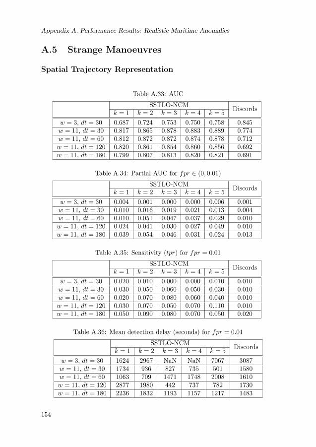
Appendix A. Performance Results: Realistic Maritime Anomalies
A.5 Strange Manoeuvres
Spatial Trajectory Representation
Table A.33: AUC
SSTLO-NCM Discordsk = 1 k = 2 k = 3 k = 4 k = 5
w = 3, dt = 30 0.687 0.724 0.753 0.750 0.758 0.845w = 11, dt = 30 0.817 0.865 0.878 0.883 0.889 0.774w = 11, dt = 60 0.812 0.872 0.872 0.874 0.878 0.712w = 11, dt = 120 0.820 0.861 0.854 0.860 0.856 0.692w = 11, dt = 180 0.799 0.807 0.813 0.820 0.821 0.691
Table A.34: Partial AUC for fpr ∈ (0, 0.01)
SSTLO-NCM Discordsk = 1 k = 2 k = 3 k = 4 k = 5
w = 3, dt = 30 0.004 0.001 0.000 0.000 0.006 0.001w = 11, dt = 30 0.010 0.016 0.019 0.021 0.013 0.004w = 11, dt = 60 0.010 0.051 0.047 0.037 0.029 0.010w = 11, dt = 120 0.024 0.041 0.030 0.027 0.049 0.010w = 11, dt = 180 0.039 0.054 0.046 0.031 0.024 0.013
Table A.35: Sensitivity (tpr) for fpr = 0.01
SSTLO-NCM Discordsk = 1 k = 2 k = 3 k = 4 k = 5
w = 3, dt = 30 0.020 0.010 0.000 0.000 0.010 0.010w = 11, dt = 30 0.030 0.050 0.060 0.050 0.030 0.010w = 11, dt = 60 0.020 0.070 0.080 0.060 0.040 0.010w = 11, dt = 120 0.030 0.070 0.050 0.070 0.110 0.010w = 11, dt = 180 0.050 0.090 0.080 0.070 0.050 0.020
Table A.36: Mean detection delay (seconds) for fpr = 0.01
SSTLO-NCM Discordsk = 1 k = 2 k = 3 k = 4 k = 5
w = 3, dt = 30 1624 2967 NaN NaN 7067 3087w = 11, dt = 30 1734 936 827 735 501 1580w = 11, dt = 60 1063 709 1471 1748 2008 1610w = 11, dt = 120 2877 1980 442 737 782 1730w = 11, dt = 180 2236 1832 1193 1157 1217 1483
154

A.5. Strange Manoeuvres
Velocity Trajectory Representation
Table A.37: AUC
SSTLO-NCM Discordsk = 1 k = 2 k = 3 k = 4 k = 5
w = 3, dt = 30 0.950 0.968 0.983 0.982 0.982 0.989w = 11, dt = 30 0.993 0.994 0.994 0.994 0.994 0.994w = 11, dt = 60 0.993 0.996 0.996 0.996 0.995 0.992w = 11, dt = 120 0.954 0.975 0.980 0.982 0.980 0.961w = 11, dt = 180 0.918 0.936 0.931 0.934 0.934 0.909
Table A.38: Partial AUC for fpr ∈ (0, 0.01)
SSTLO-NCM Discordsk = 1 k = 2 k = 3 k = 4 k = 5
w = 3, dt = 30 0.597 0.524 0.510 0.500 0.493 0.553w = 11, dt = 30 0.687 0.716 0.759 0.724 0.679 0.691w = 11, dt = 60 0.823 0.774 0.735 0.726 0.691 0.750w = 11, dt = 120 0.201 0.310 0.337 0.343 0.340 0.146w = 11, dt = 180 0.191 0.204 0.263 0.283 0.311 0.043
Table A.39: Sensitivity (tpr) for fpr = 0.01
SSTLO-NCM Discordsk = 1 k = 2 k = 3 k = 4 k = 5
w = 3, dt = 30 0.850 0.820 0.830 0.830 0.810 0.840w = 11, dt = 30 0.950 0.980 0.980 0.970 0.930 0.960w = 11, dt = 60 0.950 0.980 0.950 0.910 0.850 0.940w = 11, dt = 120 0.340 0.470 0.530 0.660 0.620 0.250w = 11, dt = 180 0.260 0.280 0.360 0.380 0.440 0.080
Table A.40: Mean detection delay (seconds) for fpr = 0.01
SSTLO-NCM Discordsk = 1 k = 2 k = 3 k = 4 k = 5
w = 3, dt = 30 79 33 37 57 39 45w = 11, dt = 30 249 107 148 196 173 108w = 11, dt = 60 396 380 446 437 435 392w = 11, dt = 120 951 1006 996 993 1014 1079w = 11, dt = 180 1623 1633 1287 1282 1197 1526
155

Appendix A. Performance Results: Realistic Maritime Anomalies
A.6 Large Vessel in Unusual Location
Multi-class anomaly detection based on vessel size.
Spatial Trajectory Representation
Table A.41: AUC
SSTLO-NCM Discordsk = 1 k = 2 k = 3 k = 4 k = 5
w = 3, dt = 30 0.966 0.977 0.939 0.979 0.979 0.974w = 11, dt = 30 0.959 0.968 0.889 0.973 0.979 0.965w = 11, dt = 60 0.967 0.946 0.873 0.963 0.965 0.959w = 11, dt = 120 0.944 0.871 0.847 0.930 0.943 0.941w = 11, dt = 180 0.873 0.795 0.779 0.878 0.893 0.890
Table A.42: Partial AUC for fpr ∈ (0, 0.01)
SSTLO-NCM Discordsk = 1 k = 2 k = 3 k = 4 k = 5
w = 3, dt = 30 0.690 0.806 0.757 0.739 0.729 0.621w = 11, dt = 30 0.727 0.730 0.716 0.520 0.669 0.620w = 11, dt = 60 0.709 0.683 0.681 0.526 0.624 0.609w = 11, dt = 120 0.754 0.660 0.593 0.510 0.506 0.501w = 11, dt = 180 0.570 0.563 0.417 0.420 0.551 0.477
Table A.43: Sensitivity (tpr) for fpr = 0.01
SSTLO-NCM Discordsk = 1 k = 2 k = 3 k = 4 k = 5
w = 3, dt = 30 0.770 0.880 0.800 0.900 0.910 0.740w = 11, dt = 30 0.760 0.780 0.790 0.600 0.790 0.730w = 11, dt = 60 0.740 0.700 0.720 0.550 0.680 0.720w = 11, dt = 120 0.800 0.670 0.670 0.520 0.520 0.680w = 11, dt = 180 0.700 0.620 0.480 0.450 0.560 0.620
Table A.44: Mean detection delay (seconds) for fpr = 0.01
SSTLO-NCM Discordsk = 1 k = 2 k = 3 k = 4 k = 5
w = 3, dt = 30 693 996 996 670 653 628w = 11, dt = 30 969 993 1206 902 941 865w = 11, dt = 60 1188 996 1364 1035 1056 1168w = 11, dt = 120 1947 1496 1977 1604 1567 1654w = 11, dt = 180 2494 2183 2760 1896 1961 2183
156

A.6. Large Vessel in Unusual Location
Velocity Trajectory Representation
Table A.45: AUC
SSTLO-NCM Discordsk = 1 k = 2 k = 3 k = 4 k = 5
w = 3, dt = 30 0.825 0.833 0.836 0.834 0.853 0.911w = 11, dt = 30 0.905 0.905 0.907 0.900 0.896 0.898w = 11, dt = 60 0.896 0.895 0.899 0.895 0.888 0.894w = 11, dt = 120 0.873 0.878 0.879 0.877 0.875 0.894w = 11, dt = 180 0.834 0.838 0.829 0.826 0.824 0.858
Table A.46: Partial AUC for fpr ∈ (0, 0.01)
SSTLO-NCM Discordsk = 1 k = 2 k = 3 k = 4 k = 5
w = 3, dt = 30 0.356 0.361 0.363 0.364 0.353 0.341w = 11, dt = 30 0.529 0.494 0.506 0.503 0.501 0.427w = 11, dt = 60 0.490 0.479 0.527 0.499 0.529 0.547w = 11, dt = 120 0.441 0.423 0.344 0.353 0.369 0.557w = 11, dt = 180 0.421 0.397 0.397 0.371 0.414 0.517
Table A.47: Sensitivity (tpr) for fpr = 0.01
SSTLO-NCM Discordsk = 1 k = 2 k = 3 k = 4 k = 5
w = 3, dt = 30 0.650 0.640 0.640 0.610 0.610 0.630w = 11, dt = 30 0.610 0.620 0.610 0.620 0.600 0.610w = 11, dt = 60 0.590 0.580 0.630 0.600 0.570 0.570w = 11, dt = 120 0.450 0.550 0.510 0.580 0.560 0.570w = 11, dt = 180 0.480 0.470 0.460 0.480 0.490 0.540
Table A.48: Mean detection delay (seconds) for fpr = 0.01
SSTLO-NCM Discordsk = 1 k = 2 k = 3 k = 4 k = 5
w = 3, dt = 30 240 262 244 411 411 296w = 11, dt = 30 733 776 870 787 1066 829w = 11, dt = 60 1595 1443 1310 1240 1308 1115w = 11, dt = 120 3176 3065 2915 2654 2376 1400w = 11, dt = 180 3818 3780 3510 3784 3696 1910
157

Appendix A. Performance Results: Realistic Maritime Anomalies
A.7 Unexpected Vessel Type/Behaviour
Multi-class anomaly detection based on vessel type.
Spatial Trajectory Representation
Table A.49: AUC
SSTLO-NCM Discordsk = 1 k = 2 k = 3 k = 4 k = 5
w = 3, dt = 30 0.927 0.940 0.944 0.946 0.947 0.948w = 11, dt = 30 0.913 0.928 0.928 0.928 0.927 0.929w = 11, dt = 60 0.903 0.918 0.920 0.921 0.919 0.917w = 11, dt = 120 0.853 0.897 0.911 0.905 0.903 0.921w = 11, dt = 180 0.835 0.875 0.887 0.891 0.890 0.908
Table A.50: Partial AUC for fpr ∈ (0, 0.01)
SSTLO-NCM Discordsk = 1 k = 2 k = 3 k = 4 k = 5
w = 3, dt = 30 0.757 0.759 0.769 0.757 0.751 0.801w = 11, dt = 30 0.750 0.741 0.737 0.720 0.707 0.751w = 11, dt = 60 0.724 0.741 0.717 0.716 0.703 0.727w = 11, dt = 120 0.690 0.686 0.699 0.693 0.687 0.737w = 11, dt = 180 0.657 0.651 0.661 0.647 0.646 0.746
Table A.51: Sensitivity (tpr) for fpr = 0.01
SSTLO-NCM Discordsk = 1 k = 2 k = 3 k = 4 k = 5
w = 3, dt = 30 0.760 0.770 0.780 0.800 0.790 0.810w = 11, dt = 30 0.770 0.760 0.770 0.750 0.750 0.780w = 11, dt = 60 0.730 0.750 0.750 0.750 0.720 0.770w = 11, dt = 120 0.690 0.700 0.730 0.720 0.730 0.770w = 11, dt = 180 0.670 0.660 0.690 0.690 0.690 0.780
Table A.52: Mean detection delay (seconds) for fpr = 0.01
SSTLO-NCM Discordsk = 1 k = 2 k = 3 k = 4 k = 5
w = 3, dt = 30 251 362 411 404 349 397w = 11, dt = 30 566 589 728 701 670 664w = 11, dt = 60 1027 926 970 899 832 845w = 11, dt = 120 1400 1459 1514 1515 1440 1582w = 11, dt = 180 1916 1893 2251 2264 2270 2038
158

A.7. Unexpected Vessel Type/Behaviour
Velocity Trajectory Representation
Table A.53: AUC
SSTLO-NCM Discordsk = 1 k = 2 k = 3 k = 4 k = 5
w = 3, dt = 30 0.859 0.865 0.875 0.883 0.881 0.873w = 11, dt = 30 0.868 0.876 0.878 0.881 0.886 0.865w = 11, dt = 60 0.874 0.859 0.864 0.874 0.881 0.871w = 11, dt = 120 0.871 0.848 0.865 0.871 0.881 0.879w = 11, dt = 180 0.853 0.844 0.865 0.872 0.878 0.868
Table A.54: Partial AUC for fpr ∈ (0, 0.01)
SSTLO-NCM Discordsk = 1 k = 2 k = 3 k = 4 k = 5
w = 3, dt = 30 0.661 0.657 0.657 0.659 0.656 0.664w = 11, dt = 30 0.656 0.653 0.654 0.654 0.650 0.650w = 11, dt = 60 0.689 0.653 0.647 0.657 0.650 0.657w = 11, dt = 120 0.669 0.674 0.670 0.661 0.671 0.694w = 11, dt = 180 0.696 0.699 0.687 0.699 0.716 0.711
Table A.55: Sensitivity (tpr) for fpr = 0.01
SSTLO-NCM Discordsk = 1 k = 2 k = 3 k = 4 k = 5
w = 3, dt = 30 0.710 0.700 0.700 0.710 0.710 0.720w = 11, dt = 30 0.690 0.690 0.690 0.690 0.690 0.690w = 11, dt = 60 0.710 0.680 0.670 0.670 0.660 0.700w = 11, dt = 120 0.680 0.680 0.690 0.670 0.690 0.720w = 11, dt = 180 0.720 0.710 0.710 0.730 0.770 0.730
Table A.56: Mean detection delay (seconds) for fpr = 0.01
SSTLO-NCM Discordsk = 1 k = 2 k = 3 k = 4 k = 5
w = 3, dt = 30 137 235 228 232 232 158w = 11, dt = 30 477 503 469 463 481 375w = 11, dt = 60 1052 928 964 1365 861 918w = 11, dt = 120 1505 1498 1583 1481 1590 1500w = 11, dt = 180 2232 2173 2170 2266 2333 2061
159

Appendix A. Performance Results: Realistic Maritime Anomalies
A.8 Overall Performance
Average performance over all the anomalous trajectories in Section A.1–A.7.
Spatial Trajectory Representation
Table A.57: AUC
SSTLO-NCM Discordsk = 1 k = 2 k = 3 k = 4 k = 5
w = 3, dt = 30 0.806 0.817 0.817 0.823 0.823 0.869w = 11, dt = 30 0.894 0.916 0.910 0.924 0.926 0.893w = 11, dt = 60 0.908 0.927 0.918 0.931 0.931 0.884w = 11, dt = 120 0.895 0.908 0.905 0.916 0.916 0.867w = 11, dt = 180 0.800 0.809 0.815 0.833 0.841 0.823
Table A.58: Partial AUC for fpr ∈ (0, 0.01)
SSTLO-NCM Discordsk = 1 k = 2 k = 3 k = 4 k = 5
w = 3, dt = 30 0.485 0.501 0.496 0.491 0.491 0.481w = 11, dt = 30 0.427 0.442 0.444 0.383 0.399 0.400w = 11, dt = 60 0.428 0.474 0.469 0.433 0.439 0.338w = 11, dt = 120 0.351 0.355 0.344 0.306 0.336 0.237w = 11, dt = 180 0.244 0.298 0.265 0.227 0.253 0.269
Table A.59: Sensitivity (tpr) for fpr = 0.01
SSTLO-NCM Discordsk = 1 k = 2 k = 3 k = 4 k = 5
w = 3, dt = 30 0.513 0.526 0.514 0.531 0.534 0.511w = 11, dt = 30 0.453 0.479 0.487 0.454 0.474 0.444w = 11, dt = 60 0.459 0.497 0.506 0.474 0.473 0.376w = 11, dt = 120 0.386 0.494 0.489 0.397 0.486 0.327w = 11, dt = 180 0.341 0.344 0.389 0.304 0.301 0.360
Table A.60: Mean detection delay (seconds) for fpr = 0.01
SSTLO-NCM Discordsk = 1 k = 2 k = 3 k = 4 k = 5
w = 3, dt = 30 760 884 471 405 1953 851w = 11, dt = 30 1188 602 851 739 649 1418w = 11, dt = 60 856 733 976 1006 1034 1205w = 11, dt = 120 1712 1319 1301 1218 1247 1497w = 11, dt = 180 2341 1875 1883 1849 1798 1657
160

A.8. Overall Performance
Velocity Trajectory Representation
Table A.61: AUC
SSTLO-NCM Discordsk = 1 k = 2 k = 3 k = 4 k = 5
w = 3, dt = 30 0.843 0.866 0.874 0.876 0.879 0.915w = 11, dt = 30 0.920 0.917 0.921 0.922 0.924 0.917w = 11, dt = 60 0.927 0.922 0.918 0.915 0.906 0.912w = 11, dt = 120 0.873 0.867 0.888 0.896 0.901 0.894w = 11, dt = 180 0.824 0.833 0.833 0.835 0.834 0.882
Table A.62: Partial AUC for fpr ∈ (0, 0.01)
SSTLO-NCM Discordsk = 1 k = 2 k = 3 k = 4 k = 5
w = 3, dt = 30 0.468 0.431 0.434 0.429 0.430 0.447w = 11, dt = 30 0.514 0.532 0.531 0.506 0.486 0.469w = 11, dt = 60 0.529 0.511 0.504 0.501 0.494 0.482w = 11, dt = 120 0.341 0.355 0.350 0.352 0.381 0.391w = 11, dt = 180 0.379 0.381 0.403 0.411 0.439 0.375
Table A.63: Sensitivity (tpr) for fpr = 0.01
SSTLO-NCM Discordsk = 1 k = 2 k = 3 k = 4 k = 5
w = 3, dt = 30 0.657 0.656 0.663 0.657 0.657 0.670w = 11, dt = 30 0.673 0.700 0.691 0.684 0.669 0.650w = 11, dt = 60 0.596 0.610 0.586 0.576 0.551 0.559w = 11, dt = 120 0.420 0.477 0.484 0.526 0.529 0.433w = 11, dt = 180 0.430 0.429 0.456 0.474 0.496 0.400
Table A.64: Mean detection delay (seconds) for fpr = 0.01
SSTLO-NCM Discordsk = 1 k = 2 k = 3 k = 4 k = 5
w = 3, dt = 30 306 291 285 322 284 275w = 11, dt = 30 484 413 432 419 426 374w = 11, dt = 60 966 845 782 879 798 608w = 11, dt = 120 1618 1504 1424 1341 1361 1051w = 11, dt = 180 1854 1958 1725 1859 1780 1454
161


References
H. Alt. The Computational Geometry of Comparing Shapes. In H. Albers,S.and Alt and S. Näher, editors, Efficient Algorithms, volume 5760 of LectureNotes in Computer Science, pages 235–248. Springer Berlin / Heidelberg, 2009.
H. Alt, B. Behrends, and J. Blömer. Approximate matching of polygonal shapes.Annals of Mathematics and Artificial Intelligence, 13(3-4):251–265, 1995.
S. Atev, G. Miller, and N. Papanikolopoulos. Clustering of Vehicle Trajector-ies. IEEE Transactions on Intelligent Transportation Systems, 11(3):647–657,September 2010.
S. Axelsson. The base-rate fallacy and the difficulty of intrusion detection. ACMTransactions on Information and System Security (TISSEC), 3(3):185–205, Au-gust 2000.
D. Barbará and C. Domeniconi. Detecting outliers using transduction and stat-istical testing. In Proceedings of the 12th Annual SIGKDD International Con-ference on Knowledge Discovery and Data Mining, 2006.
V. Barnett and T. Lewis. Outliers in Statistical Data. John Wiley and Sons, Inc.,third edition edition, 1994.
M. Berndtsson, J. Hansson, B. Olsson, and B. Lundell. Planning and Implementingyour Final Year Project - with Success!: A Guide for Students in ComputerScience and Information Systems. Springer, 2002.
N. Bomberger, B. J. Rhodes, M. Seibert, and A. Waxman. Associative learning ofvessel motion patterns for maritime situation awareness. In Proceedings of the9th International Conference on Information Fusion, 2006.
C. Brax. Anomaly Detection in the Surveillance Domain. PhD thesis, ÖrebroUniversity, 2011.
C. Brax, L. Niklasson, and M. Smedberg. Finding behavioral anomalies in publicareas using video surveillance data. In Proceedings of the 11th InternationalConference on Information Fusion, Cologne, Germany, July 2008.
163

REFERENCES
C. Brax, L. Niklasson, and R. Laxhammar. An ensemble approach for increasedanomaly detection performance in video surveillance data. In Proceedings of the12th International Conference on Information Fusion, pages 694–701, Seattle,July 2009.
C. Brax, A. Karlsson, S. Andler, R. Johansson, and L. Niklasson. Evaluating pre-cise and imprecise state-based anomaly detectors for maritime surveillance. InProceedings of the 13th International Conference on Information Fusion, 2010.
M. M. Breunig, H. P. Kriegel, R. T. Ng, and J. Sander. LOF: Identifying Density-Based Local Outliers. In Proceedings of the 2000 ACM SIGMOD InternationalConference on Management of Data, pages 93–104, 2000.
Y. Bu, L. Chen, and D. Wai-Chee Fu, A. Liu. Efficient anomaly monitoring overmoving object trajectory streams. In Proceedings of the 15th ACM SIGKDDinternational conference on Knowledge discovery and data mining, 2009.
V. Chandola, A. Banerjee, and V. Kumar. Anomaly detection: A survey. ACMComputing Surveys, 41(3):1–58, 2009.
S. Chang. Development and analysis of AIS applications as an efficient tool forvessel traffic service. In Proceedings of Ocean’04. MTS/IEEE Techno-Ocean:Bridges across the Oceans, volume 4, pages 2249–2253, 2004.
A. Dahlbom and L. Niklasson. Trajectory clustering for coastal surveillance. InProceedings of the 10th International Conference on Information Fusion, Quebeccity, Canada, July 2007.
A. Dahlbom, L. Niklasson, and G. Falkman. Situation recognition and hypothesismanagement using petri nets. In Proceedings of the 6th International Conferenceon Modeling Decisions for Artificial Intelligence, 2009.
Danish Maritime Authority. Casualty report - collision between Chinese bulkcarrier FU SHAN HAI and Cypriot container vessel GDYNIA, 2003.
H. Dee and S. Velastin. How close are we to solving the problem of automatedvisual surveillance?: A review of real-world surveillance, scientific progress andevaluative mechanisms. Machine Vision and Applications, 19(5-6):329–343,September 2008.
A. P. Dempster, N. M. Laird, and D. B. Rubin. Maximum likelihood from incom-plete data via the em algorithm. Journal of the Royal Statistical Society, seriesB, 39:1–38, 1977.
D. Devetyarov and I. Nouretdinov. Prediction with Confidence Based on a RandomForest Classifierlearning for medical diagnosis. In Proceedings of 6th IFIP WG12.5 International Conference: Artificial Intelligence Applications and Innova-tions (AIAI), volume 339 of IFIP Advances in Information and CommunicationTechnology, pages 37–44. Springer, 2010.
164

REFERENCES
R. Duda and P. Hart. Pattern Classification and Scene Analysis. John Wiley andSons, Inc., 1973.
J. Edlund, M. Grönkvist, A. Lingvall, and E. Sviestins. Rule-based situationassessment for sea surveillance. In B. V. Dasarathy, editor, Proceedings of theSPIE Multisensor, Multisource Information Fusion: Architectures, Algorithms,and Applications, volume 6242, April 2006.
J. Ekman and A. Holst. Incremental stream clustering and anomaly detection.Technical Report T2008:1, Swedish Institute of Computer Science (SICS), 2008.
E. Eskin. Anomaly detection over noisy data using learned probability distribu-tions. In Proceedings of the 7th International Conference on Machine Learning,pages 255–262, 2000.
E. Eskin, A. Arnold, M. Prerau, L. Portnoy, and S. Stolfo. A geometric frame-work for unsupervised anomaly detection. In Proceedings of the Conference onApplications of Data Mining in Computer Security, 2002.
T. Fawcett. An introduction to ROC analysis. Pattern Recognition Letters - Specialissue: ROC analysis in pattern recognition, 27(8):861–874, June 2006.
F. Fooladvandi, C. Brax, P. Gustavsson, and M. Fredin. Signature-based activ-ity detection based on bayesian networks acquired from expert knowledge. InProceedings of the 12th International Conference on Information Fusion, 2009.
J. Friedman, J. Bentley, and R. Finkel. An Algorithm for Finding Best Matchesin Logarithmic Expected Time. ACM Transactions on Mathematical Software,3(3):209–226, September 1977.
Z. Fu, W. Hu, and T. Tan. Similarity based vehicle trajectory clustering andanomaly detection. In Proceedings of IEEE International Conference on ImageProcessing, 2005.
A. Gammerman and V. Vovk. Hedging predictions in machine learning. TheComputer Journal, 50(2):151–163, 2007. ISSN 0010-4620.
D. Garagic, B. J. Rhodes, N. Bomberger, and M. Zandipour. Adaptive mixture-based neural network approach for higher-level fusion and automated behaviormonitoring. In Proceedings of the IEEE International conference on Commu-nications, 2009.
A. Gelman, J. B. Carlin, H. S. Stern, and D. B. Rubin. Bayesian Data Analysis.Chapman and Hall/CRC, 2003.
M. Goldstein. FastLOF: An Expectation-Maximization based Local Outlier detec-tion algorithm. In Proceedings of the 21st International Conference on PatternRecognition, pages 2282–2285, 2012.
165
REFERENCES
M. Goodrich and R. Tamassia. Data Structures and Algorithms in JAVA. JohnWiley and Sons, Inc., 1998.
D. Hall and S. McMullen. Mathematical Techniques in Multisensor Data Fusion.Artech House Inc., Boston, 2004.
D. Hand. Classifier technology and the illusion of progress. Statistical Science, 21(1):1–14, 2006.
D. Hawkins. Identification of Outliers. Chapman and Hall, London, 1980.
S. Ho and H. Wechsler. A martingale framework for detecting changes in datastreams by testing exchangeability. IEEE Transactions on Pattern Analysisand Machine Intelligence, 32(12), December 2010.
A. Holst, J. Ekman, and S. Larsen. Abnormality detection in event data andcondition counters on regina trains. In Proceedings of the IET InternationalConference on Railway Condition Monitoring 2006 (RCM 2006), 29-30 Novem-ber 2006, Birmingham, UK, 2006.
A. Holst, B. Bjurling, J. Ekman, Å. Rudström, K. Wallenius, R. Laxhammar,M. Björkman, F. Fooladvandi, and J. Trönninger. A Joint Statistical and Sym-bolic Anomaly Detection System Increasing Performance in Maritime Surveil-lance. In Proceedings of the 15th International Conference on Information Fu-sion, pages 1919–1926, 2012.
W. Hu, X. Xiao, Z. Fu, D. Xie, T. Tan, and S. Maybank. A system for learn-ing statistical motion patterns. IEEE Transactions on Pattern Analysis andMachine Intelligence, 28(9):1450–1464, September 2006.
J. Janssens and E. Postma. One-class classification with LOF and LOCI: Anempirical comparison. In Proceedings of the 18th Belgian-Dutch Conference onMachine Learning, 2009.
F. Johansson and G. Falkman. Detection of vessel anomalies - a bayesian networkapproach. In Proceedings of 3rd International Conference on Intelligent Sensors,Sensor Networks and Information Processing, 2007.
E. Keogh, J. Lin, and A. Fu. Hot sax: Efficiently finding the most unusual timeseries subsequence. In Proceedings of the 5th IEEE International Conference onData Mining, 2005.
S. Keogh, E.and Lonardi, C. Ratanamahatana, L. Wei, S.-H. Lee, and J. Handley.Compression-based data mining of sequential data. Data Mining and KnowledgeDiscovery, 14(1):99–129, 2007.
S. Khalid. Motion-based behaviour learning, profiling and classification in thepresence of anomalies. Pattern Recognition, 43(1):173–186, 2010.
166

REFERENCES
J. Kraiman, S. Arouh, and M. Webb. Automated anomaly detection processor. InA. Sisti and D. Trevisani, editors, Proceedings of SPIE: Enabling Technologiesfor Simulation Science VI, volume 4716, pages 128–137, July 2002.
A. Lambrou, H. Papadopoulos, and A. Gammerman. Evolutionary ConformalPrediction for Breast Cancer Diagnosis. In Proceedings of 9th InternationalConference on Information Technology and Applications in Biomedicine, pages1–4, 2009.
L. J. Latecki, A. Lazarevic, and D. Pokrajac. Outlier Detection with KernelDensity Function. In Proceedings of the 5th international conference on MachineLearning and Data Mining in Pattern Recognition, pages 61–75, 2007.
R. Laxhammar. Anomaly detection for sea surveillance. In Proceedings of the 11thInternational Conference on Information Fusion, pages 1–8, Cologne, Germany,July 2008.
R. Laxhammar. Anomaly Detection in Trajectory Data for Surveillance Applica-tions. Studies from the school of science and technology at Örebro university;19. Örebro university, 2011.
R. Laxhammar. Anomaly Detection. In V. Balasubramanian, S. Ho, and V. Vovk,editors, Conformal Prediction for Reliable Machine Learning: Theory, Adapta-tions, and Applications, Elsevier Insight Series. Morgan-Kaufmann Publishers,2014.
R. Laxhammar and G. Falkman. Conformal prediction for distribution-independent anomaly detection in streaming vessel data. In Proceedings of theFirst International Workshop on Novel Data Stream Pattern Mining Techniques,pages 47–55. Association for Computing Machinery (ACM), 2010.
R. Laxhammar and G. Falkman. Online Learning and Sequential Anomaly De-tection in Trajectories. IEEE Transactions on Pattern Analysis and MachineIntelligence, 99(PrePrints), 2013a. doi: http://doi.ieeecomputersociety.org/10.1109/TPAMI.2013.172.
R. Laxhammar and G. Falkman. Inductive Conformal Anomaly Detection for Se-quential Detection of Anomalous Sub-Trajectories. Annals of Mathematics andArtificial Intelligence: Special Issue on Conformal Prediction and its Applica-tions, September 2013b.
R. Laxhammar, G. Falkman, and E. Sviestins. Anomaly detection in sea traffic - acomparison of the gaussian mixture model and the kernel density estimator. InProceedings of the 12th International Conference on Information Fusion, pages756–763, Seattle, USA, July 2009.
J. Lee, J. Han, and X. Li. Trajectory outlier detection: A partition-and-detectframework. In Proceedings of the 24th IEEE International Conference on DataEngineering (ICDE), pages 140–149, 2008.
167

REFERENCES
M. Markou and S. Singh. Novelty detection: a review - part 1: statistical ap-proaches. Signal Processing, 83(12):2481–2497, December 2003a.
M. Markou and S. Singh. Novelty detection: a review - part 2: neural networkbased approaches. Signal Processing, 83(12):2499–2521, December 2003b.
T. Mitchell. Machine Learning. McGraw-Hill, New York, 1997.
B. Morris and M. Trivedi. A survey of vision-based trajectory learning and ana-lysis for surveillance. IEEE Transactions on Circuits and Systems for VideoTechnology, 18(8):1114–1127, August 2008a.
B. Morris and M. Trivedi. Learning and classification of trajectories in dynamicscenes: A general framework for live video analysis. In Proceedings of IEEEFifth International Conference on Advanced Video and Signal Based Surveil-lance, 2008b.
A. Naftel and S. Khalid. Classifying spatiotemporal object trajectories using un-supervised learning in the coefficient feature space. Multimedia Systems, 12(3):227–238, 2006.
H. Narasimhan and S. Agarwal. A Structural SVM Based Approach for OptimizingPartial AUC. In Proceedings of the 30th International Conference on MachineLearning, pages 516–524, 2013.
J. Owens and A. Hunter. Application of the self-organising map to trajectoryclassification. In Proceedings of the 3rd IEEE International Workshop on VisualSurveillance, 2000.
H. Papadopoulos. Inductive Conformal Prediction: Theory and Application toNeural Networks. In P. Fritzsche, editor, Tools in Artificial Intelligence. InTech,2008.
H. Papadopoulos, V. Vovk, and A. Gammerman. Conformal prediction with neuralnetworks. In Proceedings of the 19th IEEE International Conference on Toolswith Artificial Intelligence, volume 2, pages 388–395, 2007.
A. Patcha and J. Park. An overview of anomaly detection techniques: Existingsolutions and latest technological trends. Computer Networks: The Interna-tional Journal of Computer and Telecommunications Networking, 2007.
C. Piciarelli and G. Foresti. On-line trajectory clustering for anomalous events de-tection. Pattern Recognition Letters - Special issue on vision for crime detectionand prevention, 27, 2006.
C. Piciarelli, C. Micheloni, and G. Foresti. Trajectory-based anomalous eventdetection. IEEE Transactions on Circuits and Systems for Video Technology,18(11):1544–1554, November 2008.
168

REFERENCES
D. Pokrajac, A. Lazarevic, and L. Latecki. Incremental local outlier detectionfor data streams. In IEEE Symposium on Computational Intelligence and DataMining (CIDM), 2007.
F. Porikli. Trajectory Distance Metric Using Hidden Markov Model Based Repres-entation. In Proceedings of 6th IEEE International Workshop on PerformanceEvaluation of Tracking and Surveillance (PETS), 2004.
L. Portnoy, E. Eskin, and S. Stolfo. Intrusion detection with unlabeled data usingclustering. In Proceedings of ACM CSS Workshop on Data Mining Applied toSecurity (DMSA-2001), 2001.
K. Proedrou, I. Nouretdinov, V. Vovk, and A. Gammerman. Transductive Con-fidence Machines for Pattern Recognition. In Proceedings of the 13th EuropeanConference on Machine Learning, pages 381–390, 2002.
B. Rhodes. Anomaly detection and behavior prediction: Higher-level fusion basedon computational neuroscientific principles. In Sensor and Data Fusion. InTech,2009.
B. Rhodes, N. Bomberger, M. Seibert, and A. Waxman. Maritime situation monit-oring and situation awareness using learning mechanisms. In Proceedings of theMilitary Communications Conference 2005, Atlantic City, NJ, USA, October2005.
B. Rhodes, N. Bomberger, and M. Zandipour. Probabilistic associative learningof vessel motion patterns at multiple scales for maritime situation awareness. InProceedings of the 10th International Conference on Information Fusion, Que-bec, Canada, July 2007.
B. Ristic, B. La Scala, M. Morelande, and N. Gordon. Statistical analysis of motionpatterns in ais data: Anomaly detection and motion prediction. In Proceedingsof the 11th International Conference on Information Fusion, Cologne, Germany,July 2008.
M. Riveiro. Visual Analytics for Maritime Anomaly Detection. PhD thesis, ÖreboUniversity, 2011.
J. Roy. Anomaly detection in the maritime domain. In C. S. Halvorson, D. Lehr-feld, and T. T. Saito, editors, Proceedings of the SPIE Optics and Photonics inGlobal Homeland Security IV, volume 6945, Orlanda, USA, March 2008.
S. Russel and P. Norvig. Artificial Intelligence: A Modern Approach. PearsonEducation, second edition edition, 2003.
B. Schölkopf, R. Williamson, A. Smola, J. Shawe-Taylor, and J. Platt. SupportVector Method for Novelty Detection. In Advances In Neural Information Pro-cessing Systems 12, pages 582–588. 1999.
169

REFERENCES
G. Shafer and V. Vovk. A Tutorial on Conformal Prediction. Journal of MachineLearning Research, 9:371–421, March 2008.
R. R. Sillito and R. B. Fisher. Semi-supervised learning for anomalous trajectorydetection. In Proceedings of the British Machine Vision Conference (BMVC),pages 1034–1044, 2008.
B. W. Silverman. Density Estimation for Statistics and Data Analysis. Chapmanand hall, 1986.
Swedish Maritime Safety Inspectorate. Dry Cargo Vessel OOSTERBRUG -Grounding in Malmö, 2004.
N. Taleb. Fooled by Randomness: The Hidden Role of Chance in the Markets andin Life. Penguin Books, 2004.
P. Tan, M. Steinbach, and V. Kumar. Introduction to Data Mining. Addision-Wesley, 2006.
M. H. Tun, G. S. Chambers, T. Tan, and T. Ly. Maritime port intelligence usingais data. In Recent advances in security technology, 2007.
S. Urban, M. Jakob, and M. Pechoucek. Probabilistic modeling of mobile agents’trajectories. In Proceedings of the International Workshop on Agents and DataMining Interaction (ADMI), 2010.
J. van Laere and M. Nilsson. Evaluation of a workshop to capture knowledgefrom subject matter experts in maritime surveillance. In Proceedings of the 12thInternational Conference on Information Fusion, pages 171–178, 2009.
J. J. Verbeek. Mixture Models for Clustering and Dimension Reduction. PhDthesis, University of Amsterdam, Department of Computer Science, 2003.
J. J. Verbeek, N. Vlassis, and B. Kröse. Efficient greedy learning of gaussianmixture models. Neural Comput., 15(2):469–485, 2003. ISSN 0899-7667.
M. Vlachos, G. Kollios, and D. Gunopoulos. Discovering similar multidimensionaltrajectories. In Proceedings of the 18th IEEE International Conference on DataEngineering, 2002.
V. Vovk, A. Gammerman, and G. Shafer. Algorithmic Learning in a RandomWorld. Springer-Verlag New York, Inc., Secaucus, NJ, USA, 2005. ISBN0387001522.
D. Yankov, E. Keogh, and U. Rebbapragada. Disk aware discord discovery: findingunusual time series in terabyte sized datasets. Knowl. Inf. Syst., 17(2):241–262,November 2008.
A. Yilmaz, O. Javed, and M. Shah. Object tracking: A survey. ACM ComputingSurveys, 38(4), 2006.
170

REFERENCES
Z. Zhang, K. Huang, and T. T. Comparison of similarity measures for trajectoryclustering in outdoor surveillance scenes. In Proceedings of 18th InternationalConference on Pattern Recognition (ICPR), 2006.
M. Zhao and V. Saligrama. Anomaly Detection with Score functions based onNearest Neighbor Graphs. In Advances in Neural Information Processing Sys-tems 22, pages 2250–2258. 2009.
171


PUBLICATIONS IN THE DISSERTATION SERIES


PUBLICATIONS IN THE DISSERTATION SERIES 1. Berg Marklund, Björn (2013) Games in formal educational settings: Obstacles for the
development and use of learning games, Informatics. Licentiate Dissertation, ISBN 978-91-981474-0-7
2. Aslam, Tehseen (2013) Analysis of manufacturing supply chains using system dynamics and multi-objective optimization, Informatics. Doctoral Dissertation, ISBN 978-91981474-1-4
3. Laxhammar, Rikard (2014) Conformal anomaly detection: Detecting abnormal trajecto-ries in surveillance applications, Informatics. Doctoral Dissertation, ISBN 978-91-981474-2-1


V
RIKARD LAXHAMMAR Rikard Laxhammar obtained his MSc in Computer Science and Engineering in 2007 from the Royal Institute of Tech-nology, Sweden. In cooperation with Saab AB, Sweden, he was an industrial PhD student at University of Skövde, Sweden, from 2008 to 2013. Rikard has been employed by Saab since 2007 and worked part-time as a software engi-neer during his PhD studies. His main research interests and expertise are machine learning and anomaly detection. In his PhD thesis, Rikard investigates algorithms for the automated detection of abnormal motion patterns in sur-veillance applications. In the maritime domain, for exam-ple, abnormal vessel trajectories may indicate potentially dangerous situations related to sea safety and security. One of the main scientific contributions of the thesis is the de-velopment of a new method for anomaly detection, called conformal anomaly detection, which is based on the ma-chine learning theory of conformal prediction (Vovk et al.).
ISBN 978-91-981474-2-1
Dissertation Series, No. 3 (2014)
RIK
AR
D L
AX
HA
MM
AR
CO
NF
OR
MA
L AN
OM
ALY
DE
TE
CT
ION
2014