CUDA SPEED UP OPTION (FINANCIAL)PRICING BY USING BINOMIAL PRICING

TREE METHOD

By

Xiaoyu Ma

Submitted for the MSc in ComputerScience

The University of Hull

2012/9/4

ABSTRACT

Financial customers use computer technology very

widely in every aspect. In this project, there is a

analysis to compare different GPGPU technologies,

which to find the reason why chose CUDA to

accelerate option pricing operation. The content

covers from the real requirement from the evolution

of GPGPU technology to an implement of the binomial

tree algorithm. At last, it will give the

performance result for using GPGPU on the computing.

There are many different kinds of parallel computing

technology, but in financial field, which one is a

better choice for Option Pricing. Multi-core CPU is

the current main stream computing tools, but GPU

computing technology grows very quickly recent

years. Compare with traditional CPU, GPU has many

new futures making it is suitable for high-density

calculation.

TABLE OF CONTENTS

Chapter I: Introduction...........................1Chapter II: Project Background.....................3

Traditional Parallel Accelerating Technologies. .3GPGPU Parallel Accelerating Technologies........6Introduce NVIDIA GPU Hardware..................11Introduce CUDA Technology......................21Introduce Binomial Tree Method for Option Pricing...............................................30

Chapter III: Program Development..................36Program Requirement Analyze....................36Software Development Prepare...................37Software Design................................39Software Implement.............................40Software Performance Test......................63Software Improvement...........................65Self Assessment................................65Conclusion.....................................66

Appendix : Task List.............................67Appendix : Gantt Chart for Time Management........68References And Bibliography.......................75

i

C h a p t e r 1

INTRODUCTION

There are four main targets in this project.

Firstly, I will find the difference between CPU and

GPU platform on parallel computing technology. When

face the heavy computing task, the traditional

single thread CPU computing approach is limited of

its power and hardware physical character, but

parallel computing technology could provide more

computing power.

Secondly, to implement the option pricing model

based on binomial tree algorithms running on CPU and

GPU. Further more, to implement a binomial tree

algorithms code on Intel X86 CPU and on Nvidia GPU.

During the process of development, the code

optimization is very important as well, which the

optimization step should be included, especially on

the GPU side.

1

Thirdly, it is very essential that understanding how

to write hybrid code. Finally, though the

performance testing to demonstrate that GPGPU

technology has better performance to accelerate the

option pricing computing.

Higher performance means less input of computing

resource, saving more time and earning more benefit.

Especially in some crucial units or companies, such

like people working in these filed: energy,

earthquake, weather analyze, molecular dynamics, DNA

analyze and financial computing field and so on.

Therefore, finding a way to speed up these

calculations is very meaningful.

There are many accelerating technologies could be

chosen from various candidates. To choose a suitable

technology, the developer should think of their

advantages and disadvantages, and evaluate the most

accurate one for current project. The main processor

market is divided by three component including CPU

2

technology represented by Intel, GPGPU technology

represented by Nvidia and AMD, and special processer

provider like IBM, Tilera, ARM and so on. After some

years’ development, the CPU reaches a bottleneck of

performance. But recent years, GPGPU technology has

a great development, which brings the traditional

Graphics Processor to General-purpose computing.

Because GPU is used widely and good performance

under low cost, GPGPU is the most widely used

accelerating technology in many applications. This

important point is that people could get GPGPU

technology more easily than other accelerating

technologies, and get very good cost and efficiency

rate.

3

4

C h a p t e r 2

PROJECT BACKGROUND

2.1 Traditionnel Parallel Accelerating Technologies

The traditional method enhencing the computing power

is to increase the performance of CPU. When the

computer having one or two single core CPU gets the

bottleneck of performance, cluster technologies had

been developed. OpenMPI is a commoon cluster

technology to resolve computing problems. OpenMP is

the technology to use multi-core CPU fully, which

can use all cores in the CPU by a simple way.

2.1.1 OpenMPI

OpenMPI is a early technology used for clusters

application, and be used widely by many TOP500

supercomputers. This kind of accelerating technology

allows the applications runs on many computers

parallel, which could enhance all the computing

power.

5

This technology is a developed programming

technology, but it has some disadvantages including:

very difficulty of installation, complex

configuration and the compatibility between

different versions. And when the clusters become

bigger, some new problem will come out. For example,

when the number of computing node is big, it is very

important to control the delay of communications

between each node. In terms of the cost perspective,

the common customers can not afford a cluster

facility , which restrict the usage of this

technology service for more people. Therefore,

OpenMPI is not a good candidate technology for

common use.

2.1.1 OpenMP

Following by the huge development of multi-core CPU,

OpenMP was developed, which is anther open free

parallel accelerating technology. OpenMP is an

compiler API, which support multi-platform shared

memory multiprocessing programming on most processor

architectures. OpenMP programming model is portable

and scalable, which gives developers a flexible

6

interface for using parallel technology. This

accelerating technology covers from the standard

home use computer to supercomputer products.

The application could use OpenMP and OpenMPI

together, and through the extension of OpenMP for

non-shared memory computing system. For a common

computing filed, OpenMP is the easiest technology to

use. This is a diagram to describe how it works.

During the process of program, the program logic

could be parallel running automatically. The classic

example is speed up for loop. OpenMP could work well

on CPU, because of its working environment; it is

suitable for the most customers. The performance of

OpenMP depends on how many cores in the CPU. The

7

picture expresses an example for the effect of

accelerating computing.

Obviously, more number of cores mean more

performance. The main stream of compiler products

provide full support of OpenMP, and most develop

tools have the full ability of debug. Therefore,

OpenMP is a easy way to accelerate program by

parallel technology.

But OpenMP has a bottleneck of its performance.

Because the performance is based on the number of

cores, but there is a little of cores used in CPU,

which means that it is hard to enhance the power too

much on this way. Why CPU is hard to be more

8

powerful. The answer is that in current CPU

architecture, it is very complex for core design,

because CPU should process variety of kinds of task,

rather than computing. So that, too much size of

transistor be used for non-computing circuit, and

these make CPU do the computing inefficiently. This

circuit picture shows the complexity of the main

stream CPU that is produced by Intel.

From this diagram, it is clear that each core is a

complex, which offers the comprehensive functions.

Therefore, CPU can be the head of the computer

system, rather than a good calculator for computing.

Essentially, OpenMP the parallel accelerating

technology based on number of cores, has a

performance limit, despite it has some good

advantages.

9

The traditional way increasing the number of cores

in CPU has some restrictions including architecture,

production process and the final customer

requirement., there must be some new ways to

overcome these problems.

2.2 GPGPU Parallel Accelerating Technologies

Because the performance of CPU is restricted by its

architecture design when process a huge of mass

data, it is hardly to increase the number of cores

for computing. Therefore, another way is to add a

second computing processor into computing system.

GPGPU solution could satisfy this requirement, which

it is very effective as well. GPU is used for

graphic rendering work previously. It has many small

and simple structure processors. So that GPU’s

pipeline architecture is very suitable for parallel

computing. Another reason is that the price of GPU

is acceptable; rather then the professional

processors cost too much money.

10

this diagram shows the difference of design between

GPU and CPU

2.2.1 Early GPGPU Development

The general method of using GPU to do some parallel

computing is to use Shader Language, which is used

for graphic processor pipeline programming. Shader

Language is very powerful; it is the main graphics

technology that gives the power controlling GPU to

developer directly. But using Shader Language to

develop general-purpose program, which is a very

difficult thing. Firstly, this language is designed

for graphic programming; it is lack of some

important factors for general use. Secondly, there

are three main kinds of Shader Language to be chosen

for developers, including HLSL, GLSL and CG. They

are not compatible each other.

11

HLSL was created by Microsoft; it only works on

windows operations system platform with DirectX

graphic application interface. GLSL was created by

the OpenGL organization, it give developers the

ability of controlling the graphic pipeline cross-

different platforms. Actually, GLSL is used widely

covering range from graphic workstation to mobile

application such like data virtual applications,

mobile 3D games and so on. CG is created by Nvidia,

only works on its graphic processors and some game

consoles, but it is a cross platform technology as

well as GLSL. Traditionally, Shader development is

very unfriendly to developers, which makes many

obstacles to develop general-purpose application.

Therefore, the developers need a better way to use

GPU’s parallel character.

Shader Language cannot be used individually; it must

be integrated with other graphic programming

including OpenGL and DirectX. OpenGL is an open

source and free graphic programming interface. This

is big obstacle for general purpose programmer,

12

because most of the developers are not professional

graphic developer. When they decide to use GPU to

accelerate their application, they have to study new

knowledge, which will increase their workload.

Although OpenGL and DirectX are high level graphic

package technology, they are not designed for

general-purpose computing. Using graphic development

program will cause very inefficient development, so

that there are a little developers choosing this

way. In the early years, using GPU to compute

general problems was restricted in academic fields

and some top-end labs; it had not been spread widely

among most of the developers all over the world.

Therefore, some developers start to develop a new

way to release the power of graphic processor unit.

There was a reasonable approach that using these

graphic development API to develop a general-purpose

API. At first, BrookGPU a GPU project in Stanford

University and Lib Sh in Waterloo Computer Lab were

the most essential projects. They opened the door of

GPU general-purpose computing. BrookGPU was born in

13

Stanford, who submitted a concept of Stream

Programming. Furthermore, the data is boxed to set,

which is non-individual. One Kernel or multi Kernel

Running the Data consist of a Kernel chain. The

detail of parallel is hided, which means the

developer did not need to tell system some details

that what is loop or how to store data in texture

memory. BrookGPU was the original prototype of the

GPGPU, but it is not enough for satisfying

developers’ requirements. These methods did not

decline the difficulty of using them.

2.2.2 Modern GPGPU Technology

Obviously, wherever BrookGPU or Shader cannot

satisfy the huge requirements from developers. When

in the year 2005, Nvidia started to join GPGPU

field. They hired Ian Buck, a man is a GPGPU

professional people in charge of designing the CUDA

(Compute Unified Device Architecture), the first

programming API for GPGPU computing. And Nvidia

designed new GPU to support this new technology.

14

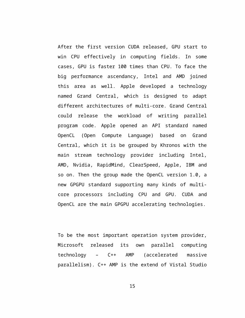
After the first version CUDA released, GPU start to

win CPU effectively in computing fields. In some

cases, GPU is faster 100 times than CPU. To face the

big performance ascendancy, Intel and AMD joined

this area as well. Apple developed a technology

named Grand Central, which is designed to adapt

different architectures of multi-core. Grand Central

could release the workload of writing parallel

program code. Apple opened an API standard named

OpenCL (Open Compute Language) based on Grand

Central, which it is be grouped by Khronos with the

main stream technology provider including Intel,

AMD, Nvidia, RapidMind, ClearSpeed, Apple, IBM and

so on. Then the group made the OpenCL version 1.0, a

new GPGPU standard supporting many kinds of multi-

core processors including CPU and GPU. CUDA and

OpenCL are the main GPGPU accelerating technologies.

To be the most important operation system provider,

Microsoft released its own parallel computing

technology – C++ AMP (accelerated massive

parallelism). C++ AMP is the extend of Vistal Studio

15

and C++ language, which it can help the developer to

adapt the parallel heterogeneous computing

environment. It uses C++ language grammar, and will

be released in the next version of Visual Studio.

Attentively, C++ AMP is an open standard like

OpenCL, which allow other compliers to integrate it.

2.2.3 Compare CUDA and OpenCL

Actually, OpenCL is an API for parallel programming

on heterogeneous computing system. During the

process of development of OpenCL, it worked on

Nvidia platform. It is used to call computing

resources on CPU and GPU, release their power to

make applications running faster.

CUDA is an original designed architecture, and its

instruments are very suitable for parallel

computing. The architecture of CUDA supports many

API such like OpenCL and DirectX and programming

languages like C, C++, Fortan and so on.

16

Because Nvidia GPU is used widely, after CUDA

released, it get much support from entertainment

providers, some important enterprise users and

academic users. For example, almost, all the video

applications are using CUDA to speed up their

performance, such like Adobe, Apple. In academic

fields, CUDA be used to accelerating Molecular

dynamics application. And in financial field, CUDA

also plays a crucial role in some products. In terms

of cost, technology support and other reasons, CUDA

is the best choice in current time for production

environment. The developer can get all information

and support from Nvidia web site, which is very

useful to spread this technology. Compared with

OpenCL support, there are sufficient documents,

example code and develop tools for learning and

developing CUDA application. Although OpenCL get

many supports of companies, there is not enough

support as much as CUDA has.

17

2.3 Introduce NVIDIA GPU Hardware

2.3.1 Introduce the early Nvidia GPU

In August 1998, Nvidia released its new generation

product Geforece 256 a revolutionary in the GPU

history. It had a most important character that

could program for geometric calculation, which means

it can reduce a huge workload for CPU. This was the

mark that the beginning of general-purpose computing

of GPU. In the next generation GPU GeForce6800, it

enhanced and expanded the power and functions of

GPU. Furthermore, vertex program started to access

texture directly, and it support dynamic branch.

Fragment program supported branch operations

including loop operation and subroutine. The new

hardware brought a great breakthrough for general-

purpose computing on GPU.

18

This diagram shows the architecture of GeForece7800

having three kinds of programmable engines for

different environment.

2.3.2 Introduce Nvidia G80 GPU

The architecture of G80 was the most important

change for using GPU to do GP computing. At the same

time, Microsoft released version 10 of DerectX,

which used unified Shader architecture to replace of

the traditional render pipeline architecture. It was

a significant change that there is only one kind of

the processor in GPU having strong ability of

computing. There are hundred of cores in the GPU,

too much more than CPU.

19

This picture introduces the G80’s unified Shader

architecture, it has 128 ALU individually could be

used for multiple purposes, and speed of computing

is much faster than CPU.

2.3.3 Introduce Nvidia G92 and GT200 GPU

The next two generation GPU were G92 and GT200,

which had some new features for general-purpose

computing. It was the first time to submit new

concepts “Gaming Beyond” and “Computing Beyond”. And

GT200 is the first GPU supporting Double-precision

float calculation, a great promotion. Because the

double precision is the necessary condition in many

science computing projects. Two new characters were

included into the products, both SIMT and shared

20

memory reduce the difficulty of the development of

general-purpose computing application.

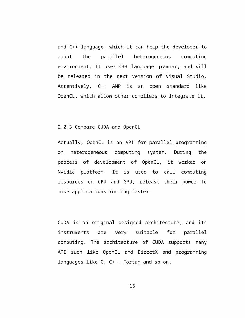
2.3.4 Introduce Nvidia Fermi GPU

Fermi (GK100) is the name of current mainstream

product of Nvidia, which was a revolutionary product

in the history of GPU. This chip has 512

microprocessors; each processor can execute a

floating point or integer instruction per clock for

one thread. There are six 64-bit memory partitions,

a 384-bit memory interface together, and supporting

a total of 6GB of GDDR5 DRAM memory. This chip

communicates with motherboard by PCI-Express

interface.

21

Fermi has 16 SM are positioned around with L2 cache.

4 SM consist of 1 GPC, and 1 SM has 32 processors.

Fermi Streaming Multiprocessor (SM)

Especially, it has third generation streaming

multiprocessor. The processor replaces the original

Shader processor, and has a fully pipelined integer

arithmetic logic unit (ALU) and floating point unit

(FPU).

22

Fermi support new floating-point standard IEEE 754-

2008, and provides the fused multiply-add (FMA)

instruction for both single and double precision

mathematic calculation. Compare with GT200, Fermi is

more accurate than it on FMA operation. And the ALU

in Fermi support full 32-bit precision for all

instructions, rather than 24-bit be supported in

GT200. The integer ALU is optimized to support 64-

bit and extended precision operation efficiently as

well. A variety of instruments containing Boolean,

shift, move, compare, convert, bit-filed extract,

bit-reverse insert and population count are

supported by hardware. In terms of these upgrade,

Fermi have a big improvement for GPGPU computing.

23

Fermi’s double precision performance up to 4.2x

faster than GT200.

Fermi could reach the peak of the performance of its

hardware, because it has two warp schedulers and two

instruction units.

Fermi enlarges the size of shared memory and L1

Cache. There are 64 KB shared memory be configured

as 48 KB of Shared memory with 16 KB of L1 cache or

24

16 KB of Shared memory with 48 KB of L1 cache. The

shared memory makes threads to cooperate in the same

block to reduces off-chip traffic greatly; this is

very significant way to increase the performance of

applications. Fermi is the first GPU to support

Error Correcting Code (ECC) for the protection of

data in memory.

2.3.5 Introduce Nvidia Kepler GPU

Kepler architecture brings some new features could

enhance the ability of calculation for HPC and many

other fields and simplify the difficulty of writing

parallel program. Kepler provides computing of over

1 TFlop double precision and 80% of DGEMM

efficiency, which is greater than Fermi’s 60 – 65%.

25

Kepler has new four kinds of new features including

Dynamic Parallelism, Hyper-Q, Grid Management Unit

and GPUDirect, which make Kepler reduce the

consummation of electricity. Furthermore, Dynamic

Parallelism could make GPU using some special

accelerating hardware path to create its new task,

and synchronous computing results, schedule task.

Hyper-Q is the technology that allow multi-host core

applications running on the same GPU, which to

decline CPU idle time and increase the utilization

of GPU. Grid Management Unit is a management and

schedule system, which make GPU to control grid more

flexibility. GPUDirect provides the ability of the

communication between the GPU in single computer and

another GPU in different environments, and do not

need to be controlled by CPU and through system

memory.

Kepler architecture incudes 15 SMX units and six 64-

bit memory.

26

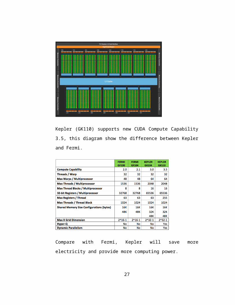
Kepler (GK110) supports new CUDA Compute Capability

3.5, this diagram show the difference between Kepler

and Fermi.

Compare with Fermi, Kepler will save more

electricity and provide more computing power.

27

Each Kepler SMX unit has 192 single precision CUDA

cores, which each core is consisted of ALU. Kepler

supports IEEE 754-2008 standard single and double

precision computing including the fused multiply-add

(FMA) operation.

One of the targets of design for Kepler is to

increase the GPU’s double precision performance

significantly, since double precision is the heart

28

of most of the HPC applications. Kepler also retains

the special function units (SFUs) for fast

transcendental operations as Fermi, and providing 8x

the number of this kinds of unit of Fermi.

2.3.6 Introduce Nvidia Tesla

Tesla is the computing module designed for server,

which could support high reliability and performance

under a low energy consummation. The main stream of

Tesla products is Tesla M-Class Computing Modules,

which are consisted of M2090, M2070/M2075 and M2050.

All the products based on Fermi architecture, have

512 cores, 448 cores and 448 cores, and built-in 6

GigaBytes, 6 GigaBytes and 3 GigaBytes memory. They

have 665 Gflops, 515 Gflops and 515 Gflops peak

double precision floating point performance

respectively.

The new generations of Tesla products are Tesla K10

and Tesla K20 based on Kepler architecture, which

29

focus on single precision computing and double

precision computing respectively. Both K10 and K20

are support the basic special characters including

ECC, L1 and L2 caches, dual DMA engines.

This is the difference of specific between Tesla K10

and K20.

2.4 Introduce CUDA Technology

2.4.1 what is CUDA

CUDA (Compute Unified Device Architecture) is a

parallel computing architecture invented by Nvidia

on its graphics processors products. It enables

increases the computing performance by using the

computing capability of the graphics processing

unit. CUDA can be used in many fields needing strong

30

computing service support, which includes Biology,

Fluid Mechanics, Molecular dynamics, Financial

analyze, Chemical formula, Finite Element Analysis

and so on. CUDA is friendly for software developers

to write parallel program running on million of

Nvidia GPU, which service for scientists and

researchers. This technology provides a variety of

support for standard programming languages including

C, C++, Fortran, Java, Python and so on.

2.4.2 CUDA History

Accompanied by the G80 the first generation product

for support CUDA released in 2006, Nvidia published

CUDA Beta version. In June 2007, CUDA 1.0 version

and Tesla series product were published. In the end

of 2007, CUDA 1.1 version released and brought some

new features such like Asynchronous execution, Data

copy, GPU SLI and so on.

31

When the GTX200 series products published, CUDA

upgraded to version 2.0. This version expanded new

features including Double-precision calculations,

profile analyzer and 3D Texture.

In Sept 2010, Nvidia published CUDA 3.2 version.

This version had a big update including new math

library contain CUSPARSE and CURAND, enhance the

efficacy of existing library. From this version,

CUDA started to support 6GB memory on board of

Quadro (a series graphics cards for professional

users) or Tesla product. Another significant

improvement is that it is the first time Nvidia

provided comprehensive developing tools to all

developers for free. These tools covered the main

platform Windows. Linux and MaxOSX. Especially, this

version corresponded Fermi architecture, the

developer could get hardware debug support.

One year later, Nvidia published the next version of

CUDA, its version number is 4.0. First, Uniform

32

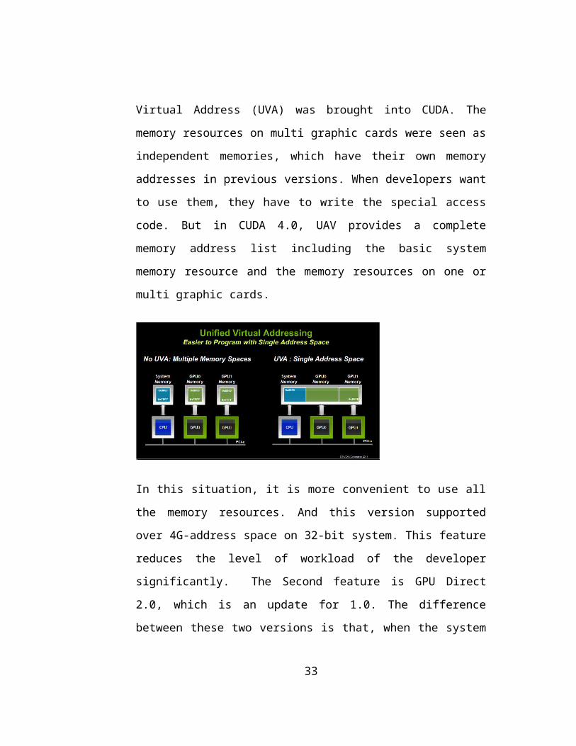
Virtual Address (UVA) was brought into CUDA. The

memory resources on multi graphic cards were seen as

independent memories, which have their own memory

addresses in previous versions. When developers want

to use them, they have to write the special access

code. But in CUDA 4.0, UAV provides a complete

memory address list including the basic system

memory resource and the memory resources on one or

multi graphic cards.

In this situation, it is more convenient to use all

the memory resources. And this version supported

over 4G-address space on 32-bit system. This feature

reduces the level of workload of the developer

significantly. The Second feature is GPU Direct

2.0, which is an update for 1.0. The difference

between these two versions is that, when the system

33

has more than one graphic card, data copy from one

to another, just need copy one time rather than

twice, the first copy from one card’s memory to main

memory and the second copy from main memory to

another card’s memory. This will save the time

consumed on data transfer and increase the

performance of the application.

The third item is a new C++ develop library named

Thrust, which includes C++ Templatized Algorithms

and Data Structures. This library could help the

developer having no experience on CUDA development

to write the program accelerated by GPU. Compared

with Standard Template Library (STL) and Intel

34

Threading Building Blocks the speed of parallel

sorting algorithms is faster 5 or 100 times than

their implements.

In 2012, Nvidia published the newest version of

CUDA. The biggest updates from the previous version

are both better support for development tools and

support the newest GK110 series product. It is the

first time for CUDA developers to get the official

Integrated Development Environment (IDE) Nsight

Eclips, which provide a good development support

under both MacOSX and Linux. For windows platform

developers, the original Visual Studio Nsight

Environment gets more function’s update. One of the

most important updates is that Nsight support single

GPU debug. In the previous version, if the developer

wants to debug the CUDA program, they need to

prepare two GPU cards, one for display and another

for debugging. The development tools performance

profiler analyzer and example code updated as well.

35

After 4 year’s growth, although some GPGPU

technologies released, like OpenCL and C++AMP, CUDA

is the most widely used technology for real

production environment.

2.4.3 Introduce CUDA Develop Tools

Nvidia provides the professional develop tools to

common developers including programmers, students,

researchers and many people who get interesting at

this technology.

In the previous versions, Windows platform get the

comprehensive develop support, but Linux and MacOSX

do not get the same treatment.

On Windows, the developer could use Night Visual

Studio Edition the official compiling and debugging

tools for Visual Studio a official C++/C IDE

generated by Microsoft, which integrated with CUDA

SDK, debugger and performance visual Profiler

together.

36

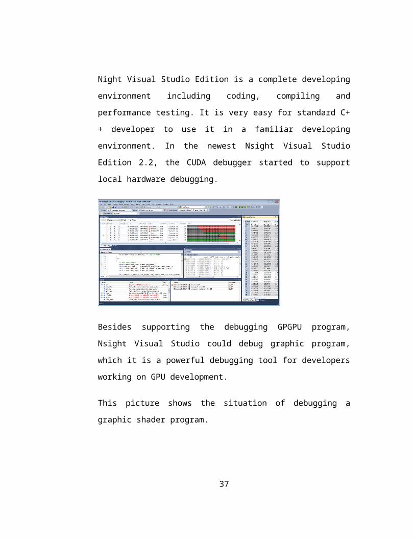
Night Visual Studio Edition is a complete developing

environment including coding, compiling and

performance testing. It is very easy for standard C+

+ developer to use it in a familiar developing

environment. In the newest Nsight Visual Studio

Edition 2.2, the CUDA debugger started to support

local hardware debugging.

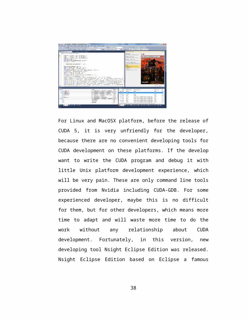
Besides supporting the debugging GPGPU program,

Nsight Visual Studio could debug graphic program,

which it is a powerful debugging tool for developers

working on GPU development.

This picture shows the situation of debugging a

graphic shader program.

37

For Linux and MacOSX platform, before the release of

CUDA 5, it is very unfriendly for the developer,

because there are no convenient developing tools for

CUDA development on these platforms. If the develop

want to write the CUDA program and debug it with

little Unix platform development experience, which

will be very pain. These are only command line tools

provided from Nvidia including CUDA-GDB. For some

experienced developer, maybe this is no difficult

for them, but for other developers, which means more

time to adapt and will waste more time to do the

work without any relationship about CUDA

development. Fortunately, in this version, new

developing tool Nsight Eclipse Edition was released.

Nsight Eclipse Edition based on Eclipse a famous

38

open source IDE used for many program languages

development.

And Nvidia also provides Profile the standard

performance test tool for free on these platforms to

CUDA developers.

Basically, the developer could write the GPGPU

program with the assist from these powerful tools,

which reduce the hard level of development.

39

2.4.4 CUDA Programming Model

The programming running on GPU is difference from on

common CPU. The CUDA thread is extremely

lightweight, which means the cost to create, destroy

threads and switch between them are very fast, and

much faster than CPU threads. Further more, the

number of CUDA threads could be thousands rather

than single digits on CPU. Therefore, using CUDA to

do parallel work is very effective.

Before the development, the developer should

understand the concept of CUDA architecture model,

which will be very helpful for their development.

CUDA includes two main models both programming model

and memory model. Both of them base on the hardware

architecture. Understanding CUDA programming model

means the developer need to understands CUDA Kernel

and Thread. Kernel is the parallel portions of an

application executed on the device that is the GPU

or other parallel computing device in the common

situation. In the same time, there is only one of

kernel executing, and there are many threads execute

40

each kernel instance. This concept is difficult to

understand. In a another words, a kernel is a

special programming code executed by all the

threads, all the threads execute the same code. Each

thread has its own ID used to be distinguished from

other threads. The ID could be used to mark memory

address and control program logic.

.

Threads are divided into many blocks a thread

running management unit in CUDA programming model. A

thread block is a batch of threads. In the block,

the threads can cooperate with each other by sharing

data through shared memory and synchronizing their

execution logic, which is a powerful feature of

CUDA.

41

.

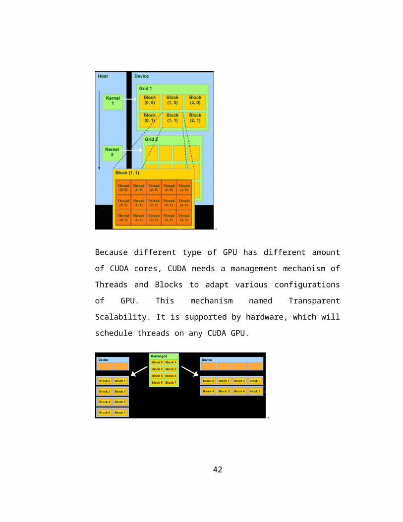
Because different type of GPU has different amount

of CUDA cores, CUDA needs a management mechanism of

Threads and Blocks to adapt various configurations

of GPU. This mechanism named Transparent

Scalability. It is supported by hardware, which will

schedule threads on any CUDA GPU.

.

42

Another essential model is CUDA memory model.

Because Nvidia GPU is designed for GPGPU computing

and graphic application, to understand the memory

model is very helpful for development. As above

known, there are five kinds of memory model on the

GPGPU system including Host (CPU) memory, Global

(device) memory, Shared memory, Local memory and

Register. Registers be used in the thread field.

There are some registers be used for per thread. All

the number of register based on the running hardware

and its architecture. For example, in Fermi

architecture, 32768 registers could be used for per

block. Local memory is an another type memory for

thread, which is located in the on board memory. In

the common situation, Local memory is a kind of

supplement for the lack of register, which means

when the number of register is not enough for use;

the complier will allocate the temp variables to

Local memory. Shared memory is the key for threads

share data in the same block; it has very fast speed

of access. Although this type memory has a high

speed, its size is restricted to very low; in Fermi

there are 48KB for per block. Global memory is the

43

on board memory, it has the biggest size among all

the five kinds of memory. Any thread could access

Global memory. Host memory is the main system

memory.

2.5 Introduce Binomial Tree Method for Option

Princing

2.5.1 Option Pricing Methods

The option is a security, which gives its owner the

right to sell or buy in a fixed number of shares,

goods or stocks at a fixed price at any time for

American Option or a fixed time for European Option.

There are two kinds of options, one is call option,

another is put option. A call option gives the

rights to buy the shares; a put option gives the

rights to sell the shares. This is the difference

between call and put option, which cause different

model design for option pricing.

44

After a long time of development of financial

market, the people invented some useful methods to

price option. For example, there are binomial tree,

Black-Scholes model and Monte Carlo simulation.

Binomial Tree pricing is the most important method.

The implement of Binomial Tree method based on the

paper <<Option Pricing: A simplified Approach>>

whose authors are Cox, Ross and Rubinstein, which

released in 1979.

2.5.2 the principle of one step of binomial tree

method

The mathematic logic will give the developer a clear

understanding about the binomial tree method for

computing option pricing. Assume using a stock to be

the example. The example stock’s current price

equals and its option price equals . The

assumption is that the validity of the option is ,

during this time the stock’s price could jump up to

a new price higher than before, or down to a new

price ( > 1, < 1). When the stock’s price

increasing, the rate of increasing of the stock’s

price is - 1; when the stock’s price decreasing,

45

the rate of decreasing of the stock’s price is 1 -

. If the stock’s price rise to , set the

assumption of option’s price is ; if the stock’s

price decline to , set the assumption of option’s

price is .

So that, there is an assumption

that combination consisted of stock and

call option for generating a value of in no risk

range. If the stock’s price rise, in the end of the

validity, the option’s value is:

If the stock’s price decline, in the end of the

validity, the option’s value is:

46

When the two values equal to each other, the

equation is:

Transform:

In this situation, this combination is risk free,

and the yield must equal to Risk-free interest rate.

If define the Risk-free interest rate equal to ,

the current value of this combination is:

And the cost of consist the combination is:

Therefore, get this formula:

Then get

47

And import the above formula

to get the final formula and though a simplify

process, then get

In this formula

From the formula above, the analyst could calculate

the option price in the beginning.

2.5.3 the principle of two or more steps of binomial

tree method

Assume the original stock’s price is ; in each

step of binomial tree, the stock’s price could rise

up to time, or down to time. Assume the Risk-

48

free interest rate is , the length of time step is

year.

Because the length of time step is rather than ,

the formula above be changed to

Repeat computing to get:

49

Finally, to get the option pricing formula:

Make sure the value of both and :

And

Therefore, could transfer the formula to:

And

50

C H A P T E R 3

PROGRAM DEVELOPMENT

3.1 Program Requirement Analyze

The most important target of this program is used to

implement a programming algorithm, which could use

GPU to accelerate the option pricing method, and

verify this way is more efficient. So that,

basically, it is very clear to understand the

target.

Basic and Necessary Implement Target

1. The Common CPU version of Binomial Tree Option

Pricing Method

2. The GPGPU version of Binomial Tree Option Pricing

Method

3. The Comparison result of the performance

4. Finding a way to integrate C++ program with CUDA

C code fragments

51

The target of add functions

1. The program should have a GUI interface, which

could display a bar chart that distinguishes the

difference of the performance for these two

calculating ways.

The development process model

Because this is an implement program of algorithm,

which it does not need a complex interface business

logic and graphic object rendering. Therefore, the

prototype development loop is very suitable for this

kind of program.

3.2 Software Development Prepare

3.2.1 make sure the development environment

Running CUDA needs a special hardware environment,

which means the graphic card supporting CUDA is a

necessary condition. Here is the configuration

development.

CPU: i3-2100 with 3GB RAM

52

GPU: GTS-450 with 1 GB RAM on board

Software environment:

Operation System: Windows7 64bit

Develop tools: Visual Studio 2010 with Nsight Visual

Studio Edition

This configuration could allow developers to debug

the CUDA program on their developing machine.

3.2.2 Version Control

Version control is very important for development.

In terms of current version control service, GIT is

much better than SVN. And there are some good GIT

service for free on the internet, for example,

Github, Bitbucket and so on. Bitbucket is chosen for

this development, which provides version control

service for private project and free.

After the process of configuration, the final web

address of git store is

git@bitbucket.org:maxiaoyu/optionspricing.git

53

3.3 Software Design

The UML of the program

54

This UML diagram shows the structure of the

implement of this CUDA algorithm. All the logic

control is located in the main. For a C++ program,

the object class is used widely, but the CUDA kernel

program is written by C language. So that, the first

55

problem need to be resolved is that make the C

kernel program working together with C++ object-

oriented code. Using a class to package a C

interface function, which is a good solution for

this problem. For example, in this program, the

class gpu1_binomial_option_pricng and

gpu2_binomial_option_pricing call the C functions

provided by gpu1_kernel and gpu2_kernel

respectively.

3.4 Software Implement

3.4.1 the main logic of environment checking

In the main function the entrance of the program,

all the logic the function call here. There are six

main steps in the program including query CUDA

device, generating option data, using CPU to

computing the option price, using GPU to computing

option price and compare the result and their

performance.

56

In the first step, it is very important to make sure

the CUDA running environment. Therefore, the

CUDA_Device class is used for this task. The

function QueryDevice will check the running

environmeny, even though the current hardware

supports it, which is a common necessary work for

all CUDA program. The program could not guarantee

the hardware and software environment satisfy the

requirement, which is the reason. CUDA API has the

special structure named cudaDeviceProp that contain

much information about hardware environment.

57

The QueryDevice function will check these items

including:

1. Compute capability: a number point the computing

function characters supported by the GPU. For

example, if the number over and equal 1.3, which

means the GPU and its driver support double

precision computing and Shared Memory atom

operation.

2. Clock rate: the core speed for GPU

3. Device Copy Overlap: this item express a

important hardware specific function, which allow

the hardware to copy data when the core computing

data. This function based on DMA technology, and

it is the basis of Stream technology a advanced

technology to improve the GPU’s performance.

4. KernelExecTimeoutEnabled: for operation system,

graphic card is very important, it cannot run a

program too long to react back to operation

system. So that, there is mechanism to prevent

the GPU dead happen, that is the kernel executing

time out mechanism. When the GPU run a code too

58

long, the operation will kill the GPU work and

reset GPU to be controlled by CPU.

5. Total Global Memory: this item show the size of

the memory on graphic card.

6. Total Constant Memory: it shows the size of

constant memory, which is a very small high speed

and read only memory. For Fermi architecture,

there is 64 KB constant memory totally.

These items could tell developers the specific

hardware performance.

The code segment:

cudaDeviceProp prop; for(int i = 0;i<DeviceCount;i++) {

HANDLE_ERROR( cudaGetDeviceProperties(&prop,i));printf(" --- general Information for Device %d ---\n",i); printf( "Name: %s\n", prop.name );printf( "Compute capability: %d.%d\n", prop.major, prop.minor ); printf( "Device support double precision: " ); if(prop.major>=2||prop.minor>=3)

support_double_precision_ = true; if(support_double_precision_)

printf( "Supported\n" );else

printf( "Unsupported\n" );

59

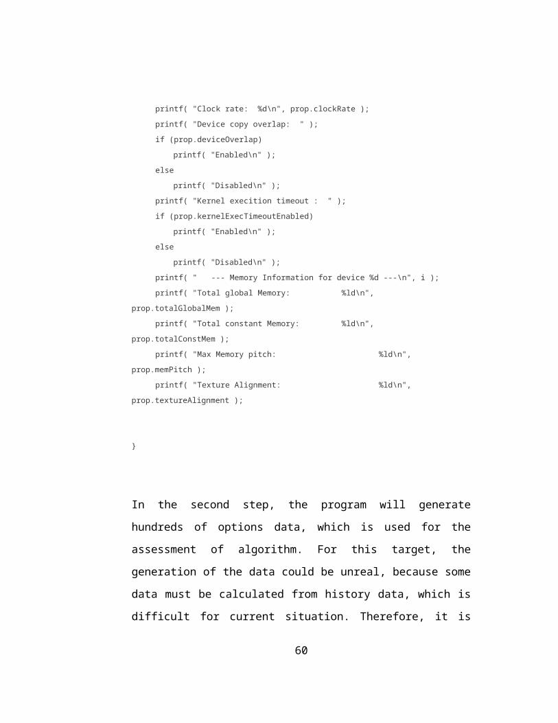
printf( "Clock rate: %d\n", prop.clockRate );printf( "Device copy overlap: " );if (prop.deviceOverlap)

printf( "Enabled\n" );else

printf( "Disabled\n" ); printf( "Kernel execition timeout : " ); if (prop.kernelExecTimeoutEnabled)

printf( "Enabled\n" ); else

printf( "Disabled\n" ); printf( " --- Memory Information for device %d ---\n", i );printf( "Total global Memory: %ld\n",

prop.totalGlobalMem );printf( "Total constant Memory: %ld\n",

prop.totalConstMem );printf( "Max Memory pitch: %ld\n",

prop.memPitch );printf( "Texture Alignment: %ld\n",

prop.textureAlignment );

}

In the second step, the program will generate

hundreds of options data, which is used for the

assessment of algorithm. For this target, the

generation of the data could be unreal, because some

data must be calculated from history data, which is

difficult for current situation. Therefore, it is

60

necessary to simulate data from a suitable range. In

terms of the current situation, there are five kinds

of data need to be estimated, including stock price,

target price for option executing time, time for how

long to keep it, Risk-free bank interest rates and

option volatility rate. The function

GenerateRandData in charge of producing a rand

number under a restriction. In this program, there

are 512 option data were generated by the program.

Assume the data under these ranges:

1. stock price (S) located in between 5.0 and 30.0

2. target price (X) located in between 1.0 and 100.0

3. the keep time located in between 0.25 and 2.0

4. set Risk-free bank interest rate to 0.06f

5. set option volatility rate to 0.10f.

because the Risk-free bank interest rate is a

different variable based on different banks and the

option volatility rate must be calculated from the

previous data, set them a fix value respectively.

61

Code Segment:

//stock price option_data[index].S = GenerateRandData(5.0f,30.0f); //target price option_data[index].X = GenerateRandData(1.0f,100.0f); //time option_data[index].T = GenerateRandData(0.25,2.0f); //No risk bank rate option_data[index].R = 0.06f; //rmuina bodong rate option_data[index].V = 0.10f;

3.4.2 the implement of CPU logic

Class CPU_Binomial_Option_Pricing implemented the

main part of CPU code for binomial tree algorithm.

Because CPU is single thread, so the 512 options

will be priced one by one, which means it is a

sequence work.

62

As above known, the binomial tree algorithm is a

backtracking method, therefore, the first task is to

computing the final option price. In terms of the

binomial tree growing type, the one step option

price could be calculated by this formula:

63

is the total number of steps, is the current

step, is the target stock price. Here is hard to

understand, to assume only one step will help

developer to make clear this formula. In one step

, , ,

Then, could expand the one step to multi-step

formula above.

So that the one step could be boxed by a function,

named calculateFinalCallOptionPrice, here is to

computing call option.

The code segments is:

double CPU_Binomial_Option_Pricing::calculateFinalCallOptionPrice(const double& S,const double& X,const double& vDt,const int& i){

double d = S * exp(vDt * (2.0 * i - NUM_STEPS)) - X; return (d > 0) ? d : 0;

}

64

After the calculation, the calculation of the one

step in the all steps is finished.

The next task is using loop to computing each result

from the previous step for option’s pricing. In the

memory, all the data of a option is stored in a

array. After the final estimate value, one option

data could do the backtracking work.

For example, here is a two-step option pricing.

If there are N steps, there must be N+1 elements be

generated in the last. And after one step of

backtracking, the number of elements be used for

computing reduce one.

So that, the second loop do the backtracking work.

Code segments:

65

for(int indexofstep = NUMBER_OF_STEPS; indexofstep > 0; indexofstep --)

for(int itemindex = 0; j <= indexofstep - 1; itemindex ++) option_cache[itemindex] = puMulDf *

option_cache[itemindex + 1] + pdMulDf * option_cache[itemindex];

In the deepest operation, the code expresses the

formula

For using CPU to calculate the option’s price, the

elements are processed one by one.

3.4.3 the implement of GPU version

The next step is to use CUDA to change the single

thread computing to parallel computing.

Obviously, the loop could be parallelization. But

using CUDA to do the parallel is a little different

from common programming.

This is the flow chart for this kind of CUDA

version.

66

In this parallel version, there are two places to be

processed in GPU, one is the calculation of

estimating data, and another one is the calculation

of each step.

Because by using the formula

could get the value directly, if the computing need

N step, the final result will have N + 1 elements.

67

Therefore, theoretically, the fast parallel approach

is that use N+1 threads to do the work. But

actually, there is a better way to release the power

of hardware.

Traditionally, there are many threads working from 0

to N+1 elements. When the size of elements is bigger

than the maximum of thread number supported by

hardware, it is impossible to finish the work. In

terms of the ability of CUDA scale ability, there is

a method could make the thread work for the

unlimited tasks.

“i” is the thread ID, can be used in the CUDA

program. If “i” expressed one common thread ID from

a limited number range, and i+1, i+2, ….. i+N (N is

68

unlimited) can express unlimited number range.

Therefore, for example, the CUDA program can use

limited thread to calculate unlimited computing

task.

Code Segment:

static __global__ void calculateFinalCallOptionPriceG1(double *call,int step, double S, double X, double vDt){

int tid = threadIdx.x; for(int i = tid; i<=step; i+=CACHE_SIZE) {

double d = S * exp(vDt * (2.0 * i - NUM_STEPS)) - X; call[i] = (d > 0) ? d : 0;

} __syncthreads();

}

This code is a kernel, must be called in a common C

environment. The CUDA organizes threads in a special

way. In the previous chapter, the content introduce

the CUDA running ways that CUDA allocate threads

into many blocks, each block has the same mode of

management of threads. But, each thread could

control its logic by distinguish its own ID.

Therefore, for this situation, there is only one

69

option data need to be generated, and the number of

steps is not bigger than the limited of the thread

restriction of the block. Using one block having

some enough threads could satisfy this requirement.

Code Segment:

calculateFinalCallOptionPriceG1<<<1,CACHE_SIZE>>>(temp_option_data,NUM_STEPS,S, X, vDt);

Explain: <<<1,CACHE_SIZE>>>, the position of 1 is

used to set the management of grid, which means how

the current grid be organized by block in 2D; the

position of CACHE_SIZE is used to set the management

of block, which means how the management of threads

in a block in 3D ways. In current setting

environment, the setting of it is that there is only

one block and this block has CACHE_SIZE (256)

threads

Based on the same way, the kernel program could do a

parallel computing for each step on the binomial

tree backtracking calculation. The CPU code could be

rewrite to the GPU code.

70

Code Segment:

static __global__ void binomialOptionsKernel1(double *call, int border, double puMulDf, double pyMulDf) { int tid = threadIdx.x; for(int i = tid; i<=border - 1; i+=CACHE_SIZE) { double a1 = puMulDf * call[i+1]; double a2 = pyMulDf * call[i]; __syncthreads(); call[i] = a1 + a2; __syncthreads(); } }

And for all the backtracking computing of an option

pricing, the code could simplify to this one.

Code Segment:

for(int i = NUMBER_OF_STEPS; i > 0; i--) { binomialOptionsKernel1<<<1,CACHE_SIZE>>>(temp_option_data, i, puMulDf, pdMulDf); }

<<<1,CACHE_SIZE>>> give CUDA core the same setting

for computing like the last operation.

71

Finally, the 512 option pricing works are processed

one by one as well. The CUDA function

“__syncthreads()” is very important for program,

which guarantee all the threads finish the executing

code before this command, then executes the next

codes. In this program, it avoids the different

threads get wrong data because of different

executing order.

Although CUDA be used in current program, does it

really play the essential role? Actually, after the

test, the speed of GPU method is slower than the

implemented by CPU. The test result of performance

will be expressed in the next chapter. Why does a

worse result after using CUDA? Is there any way to

improve the performance? Go back the check the

architecture of the GPU version code, ostensibly, it

use CUDA to accelerate the speed, but it has some

problems.

Here lists some apparent problems.

72

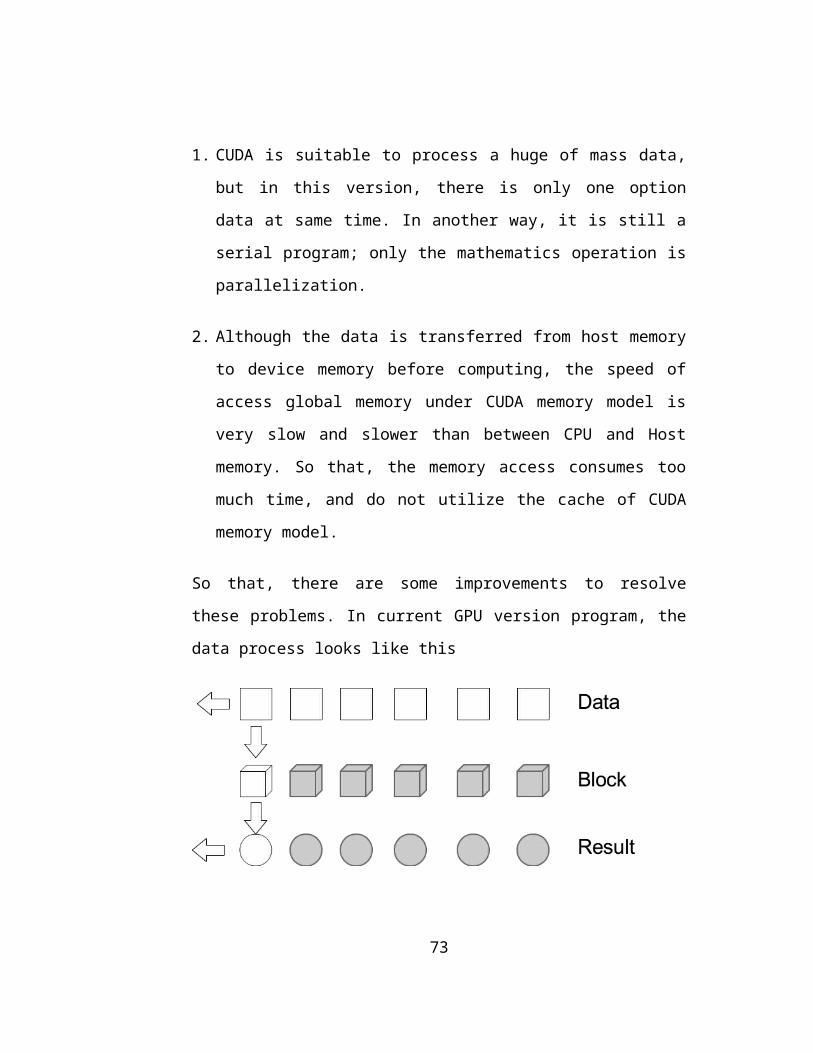
1. CUDA is suitable to process a huge of mass data,

but in this version, there is only one option

data at same time. In another way, it is still a

serial program; only the mathematics operation is

parallelization.

2. Although the data is transferred from host memory

to device memory before computing, the speed of

access global memory under CUDA memory model is

very slow and slower than between CPU and Host

memory. So that, the memory access consumes too

much time, and do not utilize the cache of CUDA

memory model.

So that, there are some improvements to resolve

these problems. In current GPU version program, the

data process looks like this

73

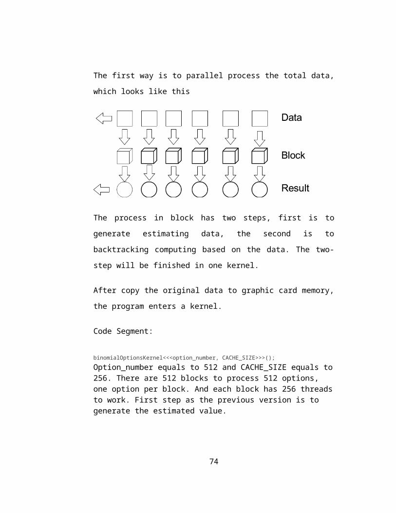
The first way is to parallel process the total data,

which looks like this

The process in block has two steps, first is to

generate estimating data, the second is to

backtracking computing based on the data. The two-

step will be finished in one kernel.

After copy the original data to graphic card memory,

the program enters a kernel.

Code Segment:

binomialOptionsKernel<<<option_number, CACHE_SIZE>>>();Option_number equals to 512 and CACHE_SIZE equals to256. There are 512 blocks to process 512 options, one option per block. And each block has 256 threadsto work. First step as the previous version is to generate the estimated value.

74

Here, this process function is not a single kernel

function, it is called in kernel function, so that,

it is a device function, and its content is the same

as the single kernel function.

Code Segment:

__device__ inline double calculateFinalCallOptionPriceG2 (double S, double X, double vDt, int i){

double d = S * exp(vDt * (2.0 * i - NUM_STEPS)) - X; return (d > 0) ? d : 0;

}

This is a device function, can only be called in

kernel functions and other device functions, and

must be executed in GPU.

Code Segment:

75

for(int i = tid; i <= NUM_STEPS; i += CACHE_SIZE)d_Call[i] = calculateFinalCallOptionPriceG2 (S, X, vDt, i);

This diagram shows how this device executed in the

GPU.

In each step of the loop, the number of the node of

the binomial tree is increasing, and the number of

GPU threads increasing as well. So that, this can

guarantee there are enough threads to support the

parallel computing.

After this step, one block has the all-estimating

data for one option, the next is to use backtracking

76

method to calculate the price of the option. As

above known, the formula

is implemented by CPU code

Call[j] = puByDf * Call[j + 1] + pdByDf * Call[j];and GPU function binomialOptionsKernel1 . In the previousGPU version, only one option and one block workingin the same time. But in this version, there are 512blocks working concurrently, so the next is to usethe hardware cache under CUDA memory model tooptimize the calculation in single one block.

There are four kinds of memory on the GPU; registersare allocated by NVCC compiler, the left areconstant memory, shared memory and global memory.Using the three kinds of memory is very important.After the first step of computing, the estimateddata stored in the global memory. In the secondstep, the algorithm should use the shared memory asmuch as possible, because its access speed is muchfaster than global memory.

Another important point is how to compute the optionprice in block concurrently. For one step of backtracking, the process likes this

77

Each node is processed by one thread. Therefore,

could guarantee to maximize the using of threads.

The memory change is like this

After one time operation, the sum of data will

reduce one. But there is a new question is that the

data stored in global memory, which means the

program will waste too much time on reading and

writing from global memory. The solution is that

move the temp computing result from global memory to

shared memory. So that, the data need to be copied

to shared memory before computing.

78

Code Segment:

callA[tid] = d_Call[c_base + tid];

The data is processed in shared memory. To keep a

high speed computing, it is helpful to prepare two

arrays in the shared memory in the current block.

79

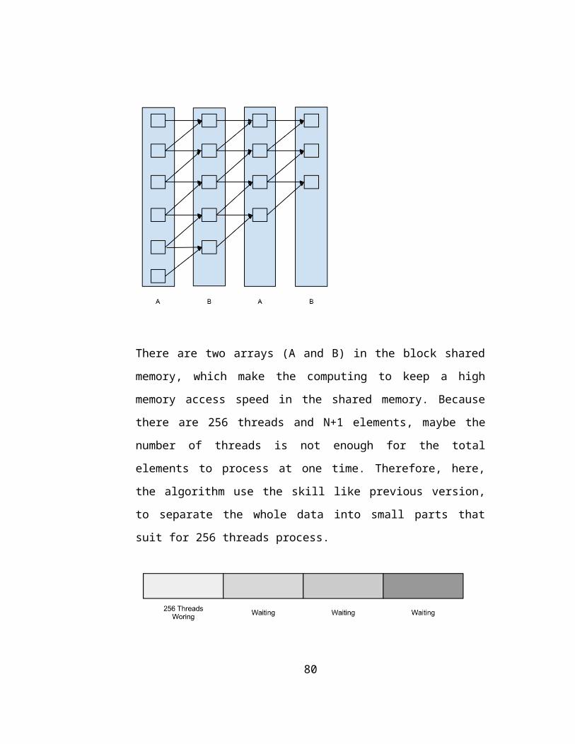
There are two arrays (A and B) in the block shared

memory, which make the computing to keep a high

memory access speed in the shared memory. Because

there are 256 threads and N+1 elements, maybe the

number of threads is not enough for the total

elements to process at one time. Therefore, here,

the algorithm use the skill like previous version,

to separate the whole data into small parts that

suit for 256 threads process.

80

Is there any way to accelerate the computing speed

from the algorithm of binomial tree again? Go back

the special binomial tree model.

Because the binomial tree is very special, there are

ways to accelerate the process speed. From this

diagram, this is a binomial tree with ten nodes. The

first thing need to be clear is that make sure the

direction of computing is from left to right.

81

If get the result of node 5 that needs node 1 and 2,

expand it to node 6, which needs node 2 and 3. So

that the node 5 and the node 6 share the node 2.

If get the result of node 8 that needs node 1,2,3,5

and 6. And getting the result of 9 needs 2,3,4,6 and

7. There is a principle here that if the level of

the two nearest nodes increases one level, the left

node will share its children nodes besides the left

children to its right node.

Therefore, in each block operation, the program do

not need to compute the node value one level by one

level, the height of each part of the level could

82

higher than two. So the abstract algorithm image

looks like this.

For the previous design, assume there are two

threads in one block, the image is

For the second design having multi-level computed

by many thread could provides more powerful

computing ability, which looks like this

83

Obviously, this design increase the capacity of data

in each step, because the computing happens at

shared memory, which guarantee the access speed. In

the shared memory, the computing model looks like

this

84

The computing happens at the two shared memory

spaces respectively.

Code Segment:

for(int i = NUMBER_OF_STEPS; i > 0; i -= CACHE_DELTA) for(int window_base = 0; window_base < i; window_base += CACHE_STEP){

int window_begin_point = min(CACHE_SIZE - 1, i - window_base);int window_end_point = window_begin_point - CACHE_DELTA;__syncthreads();if(tid <= window_begin_point)

shared_cacheA[tid] = base_point_in_All_Call[window_base + tid];

for(int windowitemindex = window_begin_point - 1; windowitemindex >= window_end_point;)

{__syncthreads();shared_cacheB[tid] = puMulDf * shared_cacheA[tid + 1]

+ pdMulDf * shared_cacheA[tid];windowitemindex --;__syncthreads();shared_cacheA[tid] = puMulDf * shared_cacheB[tid + 1]

+ pdMulDf * shared_cacheB[tid];windowitemindex --;

}__syncthreads();if(tid <= window_end_point)

base_point_in_All_Call[window_base + tid] = shared_cacheA[tid];}

85

After performance testing, the result is better than the previous version and CPU version.

3.5 Software Performance Test

On GTX450

CPU GPU1 GPU20

1

2

3

4

5

6

Running Time

Running Time

CPU, GPU1 and GPU2 spend 4s, 5.565s and 0.243s

respectively.

Obviously, GPU2 has a great performance superiority,

which it is faster 16.46 times than CPU and 22.90

times than GPU1 respectively. So that, this result

86

maybe verify the design defect of GPU1, which means

memory read and write operation spend too much time.

The next is to use Nvidia Compute Visual Profiler

the official performance checking tool to check the

detail of the code among CPU, GPU1 and GPU2 the

three implements of binomial tree.

By using Nvidia Compute Visual Profiler, more

details of the difference of the performance between

the two versions GPU1 and GPU2 will be shown.

On GTX560

CPU GPU1 GPU20

0.51

1.52

2.53

3.54

4.5

Running Time

Running Time

87

GPU1 get a better performance, because GTX560 has

384 cores, which is double number of cores than

GTX560. More cores means more block runs at the same

time.

The GPU Time Compare Result

This diagram shows that GPU2 version uses too much

GPU time than GPU1 version, which means GPU2 version

the GPU hardware is used fully.

The CPU Time Compare Result

The Compare of the instructions executed

88

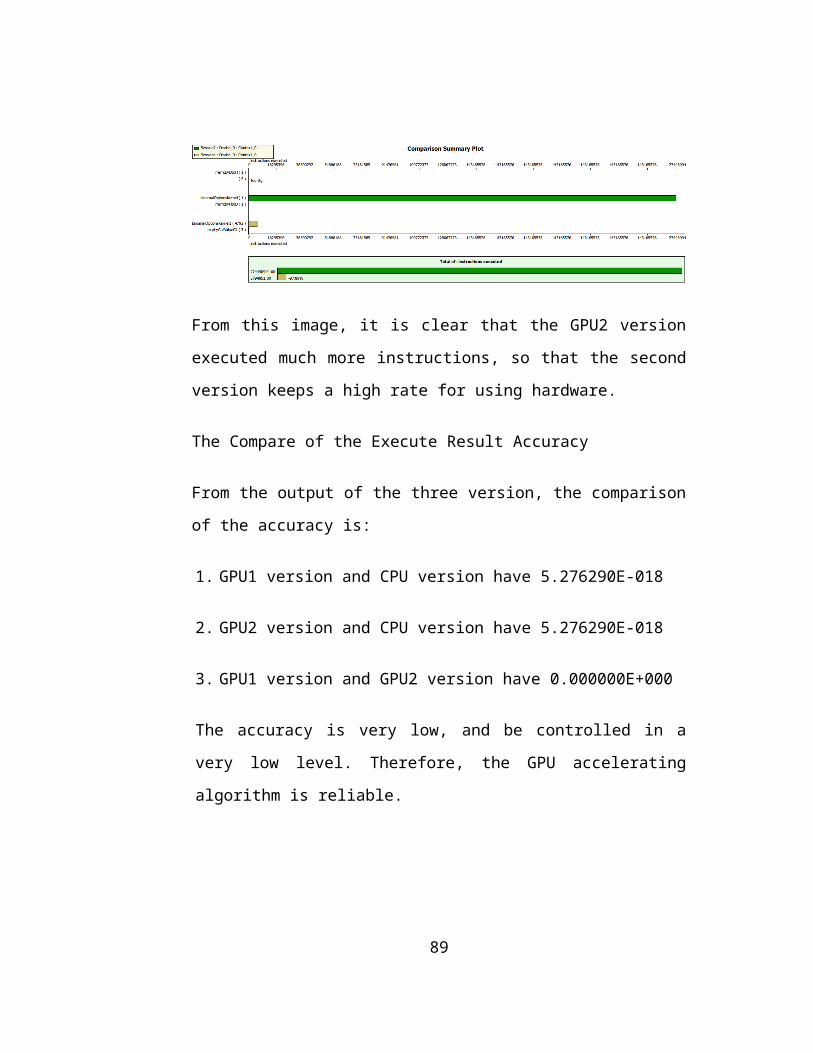
From this image, it is clear that the GPU2 version

executed much more instructions, so that the second

version keeps a high rate for using hardware.

The Compare of the Execute Result Accuracy

From the output of the three version, the comparison

of the accuracy is:

1. GPU1 version and CPU version have 5.276290E-018

2. GPU2 version and CPU version have 5.276290E-018

3. GPU1 version and GPU2 version have 0.000000E+000

The accuracy is very low, and be controlled in a

very low level. Therefore, the GPU accelerating

algorithm is reliable.

89

3.6 Software Improvement

Although the algorithm has been implemented and

running on the current main stream GPU architecture,

there are still some placement could be improved.

First, in the real situation, the number of option

is hard to control, sometime it is big, and sometime

it is small. When it is big, this algorithm is fine,

but when it is small, the hardware resource will

waste too much. Because Fermi architecture cannot

execute multi-kernel concurrently, so this problem

cannot be correct on this architecture. But in the

Kepler K110 architecture, this point could be

improved, which Kepler could launch multi-kernel to

optimize the implement of the algorithm.

Better GPU has better performance, current hardware

is GTX450 having 192 cores, but if executes on

GTX560 having 384 cores will get better time.

Because more cores means more block could run

concurrently.

90

3.7 Self Assessment

This project is a personal work. This project stands

at above both financial knowledge and computer

programming technology. Before the development, I

had to self-teaching the financial knowledge, and

read many references. To be a computer science

student, learning an untouched course is very

difficult, especially integrated with much math

information. Finally, I understood the knowledge.

It is the first time for me to develop a GPU

program, which is different from the common graphic

C++ program or other web, mobile application. This

kind of application focus on the data operation and

the implement of algorithm, therefore, it does not

have beautiful user interface. During the process of

the application, I understand the GPU programming

deeply, and understand how develop a real GPGPU

program. By the way, this project give me the fist

experience on financial computing project

development.

91

3.8 Conclusion

In this chapter, though diagram, code segments and

description to show three different kinds of

implement of the binomial tree option pricing

algorithm. Depends on the CUDA technology, the

traditional serial CPU algorithm could be

accelerated by GPGPU computing technology. Finally,

by the performance test verified GPGPU technology is

very helpful for accelerating Option Pricing by

binomial tree method.

92

A p p e n d i c e s

4.1 Task list

This a cross-filed project, there are many task need

to do. Before software development, the first thing

is learning the financial knowledge.

Development Prepare Task

1. Studying Financial Background knowledge

a) Basic Concept

b) The relationship between different area

2. Studying Option Knowledge

a) Basic Concept

b) Calculation Method

i. Binomial Tree Method

ii. Black-Sholes Method

3. Studying CUDA

93

a) Basic Knowledge

b) Programming Model

4. Algorithm Design

a) CPU version Design

b) GPU version Design

Development Task

1. Requirement Design

a) Make Clear Target

b) Understand how to implement

2. Software Design

a) Program Structure Design

3. Software Implement

a) CPU implement

b) GPU implement

c) Performance Compare

94

4.2 Gantt Chart for Time Management

95

REFERENCES AND BIBLIOGRAPHY

[1] John C. Hull, 2005, FUNDAMENTALS OF FUTURES AND

OPTIONS MARKETS

[2] John C. COX, Stephen A. ROSS, Mark RUBUNSTEIN,

July 1979, OPTION PRICING : A SIMPLIFIED

APPROACH, Massachusetts Institute of Technology,

Cambridge, MA 02139, USA Stanford University,

Stanford, CA 94305, USA, Yale University, New

Haven, CT 06520, USA, University of California,

Berkeley, CA 94720, USA

[3] Nathan Whitehead, Alex Fit-Florea, 2011,

Precision & Performance : Floating Point and

IEEE 754 Compliance for NVIDIA GPUs

[4] Nvidia Corporation, May 2011, Compute Visual

Profiler

[5] Nvidia Corporation, 2008, CUDA Programming Model

Overview

[6] Nvidia Corporation, 2006, CUDA Programming Model

Overview

96

[7] David Kirk, 2006-2008, NVIDIA and Web-mei Hwu,

Chapter 2 CUDA Programming Model

[8] Nvidia Corporation, 2011, The ‘Super’ Computing

Company From Super Phones to Super Computers

[9] Tim C. Schroeder, 2011, Peer-to-Peer & Unified

Virtual Addressing CUDA Webinar

[10] Peter N. Glaskowsky, 2009, NVIDIA’s Fermi : The

First Complete GPU Computing Architecture

[11] Nvidia Corporation, August 2011, TESLA M-CLASS

GPU COMPUTING MODULES

[12] Nvidia Corporation, March 2012, SDK CODE SAMPEL

GUIDE TO NEW FEATURES IN CUDA TOOLKIT v4.2

[13] Nvidia Corporation, January 2012, GETTING

STARTED WITH CUDA SDK SAMPLES

[14] Nvidia Corporation, May 2012, NVIDIA CUDA C

Programming Guide

[15] Nvidia Corporation, April 2012, NVIDIA CUDA

GETTING STARTED GUIDE FOR MICOSOFT WINDOWS

97

[16] Nvidia Corporation, January 2012, CUDA API

REFERENCE MANUAL Version 4.1

[17] Nvidia Corporation, May 2011, FERMI

COMPATIBILITY GUIDE FOR CUDA APPLICATIONS

[18] Nvidia Corporation, May 2011, TUNING CUDA

APPLICATIONS FOR FERMI

[19] Nvidia Corporation, 2012, NVIDIA’s Next

Generation CUDA Compute Architecture : Kepler

GK110

[20] Nvidia Corporatin, May 2012, KEPLER

COMPATIBILITY GUIDE FOR CUDA APPLICATIONS

[21] Jason Sanders, Edward Kandrot, 2010, CUDA BY

EXAMPLE An Introduction to General-Purpose GPU

Programming [source code] book.h

98

4