The binomial transform and the analysis of skip lists�

Patricio V. Pobletea,∗,1, J. Ian Munrob, Thomas Papadakisc,2

aDepartment of Computer Science, University of Chile, Casilla 2777, Santiago, ChilebDepartment of Computer Science, University of Waterloo, Waterloo, Ont., Canada N2L 3G1cLegato Systems (Canada) Inc, 3390 South Service Road, Burlington, Ont., Canada L7N 3J5

Abstract

To any sequence of real numbers 〈an〉n�0, we can associate another sequence 〈as〉s �0, which Knuth calls its binomial transform.This transform is defined through the rule

as = Bsan =∑n

(−1)n( s

n

)an.

We study the properties of this transform, obtaining rules for its manipulation and a table of transforms, that allow us to invert manytransforms by inspection.

We use these methods to perform a detailed analysis of skip lists, a probabilistic data structure introduced by Pugh as an alternativeto balanced trees. In particular, we obtain the mean and variance for the cost of searching for the first or the last element in the list(confirming results obtained previously by other methods), and also for the cost of searching for a random element (whose variancewas not known).

We obtain exact solutions, although not always in closed form. From them we are able to find the corresponding asymptoticexpressions.

Keywords: Binomial transform; Skip lists; Analysis of algorithms

� This research was supported in part by the Natural Sciences and Engineering Research Council of Canada under Grant no. A-8237, the InformationTechnology Research Centre of Ontario, and FONDECYT(Chile) under Grants 1950622 and 1981029.The publisher apologizes to the authors and editors for the unacceptable delay in printing this article. This happened due to a change in supportsystems for the journal and represents an exceptional case for which the publisher, nevertheless, takes full responsibility.∗ Corresponding author.

E-mail address: ppoblete@dcc.uchile.cl (P.V. Poblete).1 Part of this work was done while the author was on sabbatical at the University of Waterloo.2 Part of this work was done while the author was a post doctoral fellow at the University of Waterloo.

P.V. Poblete et al.

1. Introduction

The inversion formula

an =∑k

(−1)k(

n

k

)bk ⇐⇒ bn =∑

k

(−1)k(

n

k

)ak (1)

plays an important rôle in the analysis of some algorithms and data structures, and in the solution of many combinatorialproblems [19,8].

In [11] Knuth used this relation to define a transform, mapping sequences of real numbers onto sequences of realnumbers. Even though the experience with other similar transforms indicates that they can be powerful tools, in thiscase the concept does not seem to have been developed, and the literature is lacking in tables of binomial transforms,rules for their manipulation, inversion, etc.

In this paper, we develop the theory of the binomial transform, and show how it can be applied to analyze theperformance of skip lists, a probabilistic data structure introduced by Pugh [18,14].

Using the binomial transform, we give alternative derivations for some known results and solve an open problem.Our results give exact expressions for the relevant performance measures, as functions of n (the number of keys in thedata structure). This is useful, because it allows us to check the consistency of our solutions, by comparing them to thevalues obtained by numerical evaluation of the corresponding recurrence equations for small values of n. From theseexact expressions it is easy to obtain asymptotic expressions. As a possible drawback, the manipulations required forthe analysis may become complicated, and often require the use of a symbolic algebra system.

2. Notation

We generally follow the notational conventions of [8]. In particular, for any Boolean expression C, [C] denotes afunction that has the value 1 if C is true, and 0 otherwise. If �(x) is the Gamma function, �(x) is its logarithmic derivative(�(x) = �′(x)/�(x)). The harmonic numbers are defined as Hn =∑1�k �n

1k

. Equivalently, Hn = �(n+1)+�, where

� = 0.5772 . . . is Euler’s constant. Asymptotically, Hn = ln n+ �+O( 1n). The harmonic numbers can be generalized

to noninteger arguments by the formula Hx = ∑k �1 ( 1k− 1

k+x), and it can be shown that Hx = �(x + 1) + �. The

second-order harmonic numbers H(2)n are defined as H

(2)n =∑1�k �n

1k2 , and their limiting value is H

(2)∞ = �2

6 . The

rising and falling factorial powers are defined as xn = x(x + 1) · · · (x + n − 1) and xn = x(x − 1) · · · (x − n + 1),respectively. They can be extended to negative exponents by means of the relation x−n = 1/(x−1)n. In addition to thestandard binomial coefficients, we also use a notation for the symmetric binomial coefficients (i, j) = (i+j

i

) = (i+jj

).

The equivalent formula (x, n) = (x + 1)n/n! extends this to the case of one noninteger argument. The notation

Qr(m, n) denotes the Q functions [11], defined as Qr(m, n) = ∑0� j �n(j, r)

nj

mj , for r �0. The notation B(x, y)

denotes the Beta function (B(x, y) = �(x)�(y)/�(x + y)). The operator Dx denotes a partial derivative with respectto x. Whenever the variables p and q are used, it will be assumed that p + q = 1. Finally, throughout the paper, eachoccurrence of the symbol �(·) will denote a (possibly different) periodic function, usually of very small amplitude andmean 0 (see Section 3.8).

3. The binomial transform

3.1. Definition

For any sequence of real numbers 〈an〉n�0 we define its binomial transform as the sequence 〈as〉s �0, where

as = Bsan =∑n

(−1)n(

s

n

)an. (2)

Note that, since s is a nonnegative integer, the binomial coefficients vanish for n < 0 or n > s. Therefore the actualrange of the summation is really 0�n�s, but we prefer to write it as an unconstrained sum to simplify notation.

P.V. Poblete et al.

Furthermore, we will always assume that an = 0 for all n < 0, and as = 0 for all s < 0. For example, when we write“an = 1” we actually mean “an = [n�0].”

Another interesting formulation can be given if we rewrite the definition of the transform using the operators Zan =a0, Ean = an+1, Ian = an and �an = (E− I)an = an+1 − an. In terms of these operators, we have

Bs ≡ Z∑k

(−1)k(

s

k

)Ek ≡ Z(I− E)s ≡ Z(−�)s .

3.2. Inverse transform

Because of the inversion formula (1), it is easy to see that we can recover an from as by using the same formula (2),with the rôles of n and s reversed. Thus,

an = Bnas =∑s

(−1)s(

n

s

)as . (3)

3.3. Relation with other transforms

For any sequence of real numbers 〈an〉n�0, its Poisson Transform [7,15] can be defined as

Pxan = e−x ∑n�0

an

xn

n!(this corresponds to the case m = 1 in [7,15]). For any function f (x), its Mellin Transform [12,4,6] is defined as

Msf (x) =∫ ∞

0f (x)xs−1 dx.

It is not hard to prove that the following formal identity holds between these two transforms and the binomial transform:

Bsan = 1

�(−s)M−sPxan.

The binomial transform is also related to the exponential generating function. If A(z) is the egf of the sequence an,then ezA(−z) is the egf of the transformed sequence.

3.4. Rules for the manipulation of binomial transforms

The following is a list of useful rules for the manipulation of binomial transforms. For the sake of clarity and easeof reference, the proofs for these properties have been collected in Appendix A.R1. Bs(�an + �bn) = �Bsan + �Bsbn (Linearity).

R2. Bsan+1n+1 = − as+1

s+1 .

R3. Bs

∑0�k<n ak = −as−1, Bs

∑0�k �n ak = as − as−1,

Bsan−1 = −∑0� t<s at , Bs(an − an−1) =∑0� t � s at .

R4. Bs1

n+1

∑0�k �n ak = as

s+1 , Bsan

n+1 = 1s+1

∑0� t � s at .

R5. Bs(an+1 − an) = −as+1, Bsan+1 = as − as+1.

R6. Bs(nk)an−k = (−1)k(

sk)as−k (or equivalently, Bsn

kan−k = (−1)kskas−k).

R7. Bsnan = s(as − as−1), Bsn(an − an−1) = sas .

For the following three properties, recall our convention that p + q = 1:

R8. Bs

∑k (

nk)pkqn−kak = psas .

R9. Bs

∑k (

nk)pkqn−kakbn−k =∑k (

sk)pkqs−kakbs−k.

P.V. Poblete et al.

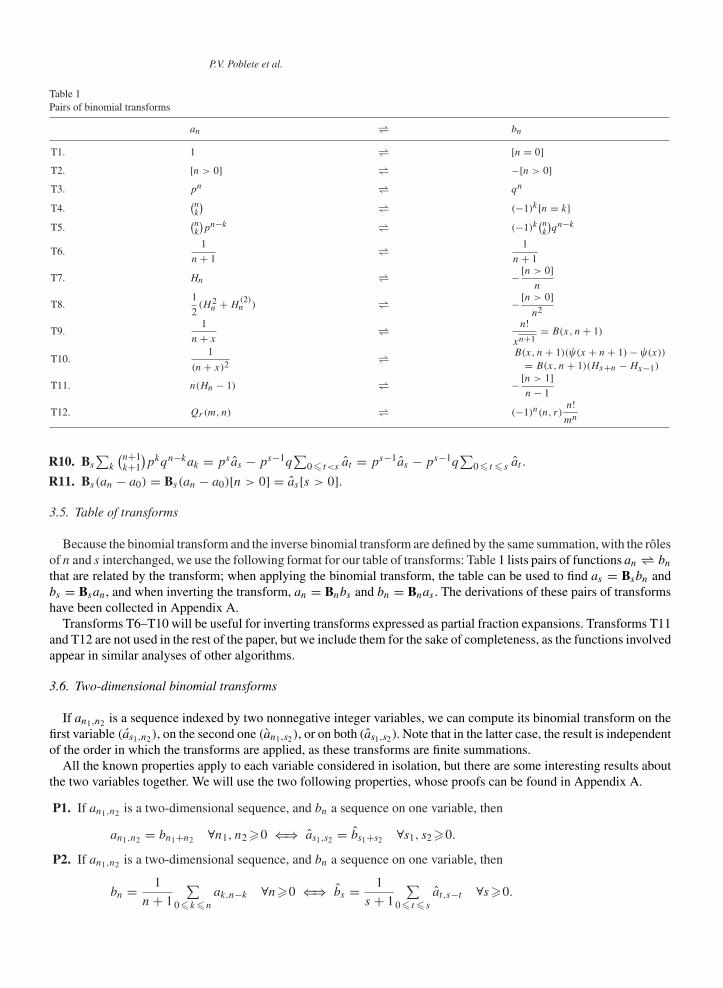
Table 1Pairs of binomial transforms

an ⇀↽ bn

T1. 1 ⇀↽ [n = 0]T2. [n > 0] ⇀↽ −[n > 0]T3. pn ⇀↽ qn

T4.(nk

)⇀↽ (−1)k[n = k]

T5.(nk

)pn−k ⇀↽ (−1)k

(nk

)qn−k

T6.1

n+ 1⇀↽

1

n+ 1

T7. Hn ⇀↽ −[n > 0]n

T8.1

2(H 2

n +H(2)n ) ⇀↽ −[n > 0]

n2

T9.1

n+ x⇀↽

n!xn+1

= B(x, n+ 1)

T10.1

(n+ x)2⇀↽

B(x, n+ 1)(�(x + n+ 1)− �(x))

= B(x, n+ 1)(Hx+n −Hx−1)

T11. n(Hn − 1) ⇀↽ −[n > 1]n− 1

T12. Qr(m, n) ⇀↽ (−1)n(n, r)n!mn

R10. Bs

∑k

(n+1k+1

)pkqn−kak = psas − ps−1q

∑0� t<s at = ps−1as − ps−1q

∑0� t � s at .

R11. Bs(an − a0) = Bs(an − a0)[n > 0] = as[s > 0].

3.5. Table of transforms

Because the binomial transform and the inverse binomial transform are defined by the same summation, with the rôlesof n and s interchanged, we use the following format for our table of transforms: Table 1 lists pairs of functions an ⇀↽ bn

that are related by the transform; when applying the binomial transform, the table can be used to find as = Bsbn andbs = Bsan, and when inverting the transform, an = Bnbs and bn = Bnas . The derivations of these pairs of transformshave been collected in Appendix A.

Transforms T6–T10 will be useful for inverting transforms expressed as partial fraction expansions. Transforms T11and T12 are not used in the rest of the paper, but we include them for the sake of completeness, as the functions involvedappear in similar analyses of other algorithms.

3.6. Two-dimensional binomial transforms

If an1,n2 is a sequence indexed by two nonnegative integer variables, we can compute its binomial transform on thefirst variable (as1,n2), on the second one (an1,s2), or on both (as1,s2 ). Note that in the latter case, the result is independentof the order in which the transforms are applied, as these transforms are finite summations.

All the known properties apply to each variable considered in isolation, but there are some interesting results aboutthe two variables together. We will use the two following properties, whose proofs can be found in Appendix A.

P1. If an1,n2 is a two-dimensional sequence, and bn a sequence on one variable, then

an1,n2 = bn1+n2 ∀n1, n2 �0 ⇐⇒ as1,s2 = bs1+s2 ∀s1, s2 �0.

P2. If an1,n2 is a two-dimensional sequence, and bn a sequence on one variable, then

bn = 1

n+ 1

∑0�k �n

ak,n−k ∀n�0 ⇐⇒ bs = 1

s + 1

∑0� t � s

at,s−t ∀s�0.

P.V. Poblete et al.

3.7. Numerical computation of binomial transforms

In the course of solving a problem using binomial transforms, one is often performing complex manipulations, eithermanually or with the aid of a symbolic algebra system, or more likely with a mix of the two. As a consequence, oneis likely to feel (or indeed to be) error prone, and it is very helpful to be able to evaluate some functions and theirtransforms numerically, as a consistency check. However, it may be cumbersome to use the definition of the transformfor this computation, as it involves binomial coefficients that may become quite large. We will see that there is a simplerecurrence that will let us simplify this process.

Using rule R5 and replacing s by s − 1 and n by n+ k, we have that Bsan+k = Bs−1an+k − Bs−1an+k+1. DefiningAs,k = Bsan+k , we have the recurrence As,k = As−1,k − As−1,k+1, with the boundary condition A0,k = ak . Thetransform as can be obtained as as = As,0.

For example, the following table illustrates numerically the relation Bs[n>0]

n= −Hs . Note that the input sequence

〈an〉n�0 goes in the first row, and the output sequence 〈as〉s �0 appears in the first column.

If we want to compute the as sequentially, a single array suffices to implement this process. The following algorithmcomputes a0, a1, . . . given a0, a1, . . . using an array L, that satisfies the invariant L[k] = As−k,k:

for s = 0, 1, . . . doL[s] ← as

for k = s − 1, s − 2, . . . , 0 doL[k] ← L[k] − L[k + 1]

as ← L[0]

3.8. Oscillating functions

Consider the function

1

s + �,

where � is an imaginary parameter. From transform T9, we know that its inverse is

B(�, n+ 1) = n!�n+1

,

which is asymptotically a periodic function of log n, since B(�, n+ 1) ∼ �(�)e−� ln n.In our applications, we will encounter functions of the form

Fn = 1

ln p

∑k �=0

B(�k, n+ 1) = Bn

1

ln p

∑k �=0

1

s + �k

,

where �k = 2�ikln p

, p is a real parameter (0 < p < 1), and the summation ranges over all negative and positive integers.

Besides this basic function, several others related to it will appear, and it will be convenient to define a family

P.V. Poblete et al.

of functions

F [r]n =1

ln p

∑k �=0

�rkB(�k, n+ 1)

such that

F [r]s =1

ln p

∑k �=0

�rk

s + �k

.

This way of generalizing Fn is a natural one, if we observe that multiplying n!/�n+1k by �r

k simply cancels or adds theappropriate factors, yielding

F [r]n =1

ln p

∑k �=0

n!(�k + r)n−r+1

.

The three values of r that will appear often are 1, 0 and −1. The corresponding functions and their transforms are:

F[1]n = 1

ln p

∑k �=0

�kB(�k, n+ 1), F[1]s = 1

ln p

∑k �=0

�k

s + �k

,

F[0]n = 1

ln p

∑k �=0

B(�k, n+ 1), F[0]s = 1

ln p

∑k �=0

1

s + �k

,

F[−1]n = 1

ln p

∑k �=0

B(�k, n+ 1)

�k − 1, F

[−1]s = 1

ln p

∑k �=0

1

(�k − 1)(s + �k).

Note that, by using a partial fraction expansion, we can rewrite F[−1]s as

F [−1]s = 1

s + 1

1

ln p

∑k �=0

(1

�k − 1− 1

s + �k

).

But 1ln p

∑k �=0

1�k−1 = 1

2 + pq+ 1

ln p(as can be seen by setting s = −1 in expansion E1 in Appendix A, and using the

fact that∑

k �=01

�k+1 = −∑

k �=01

�k−1 ), so we have that

F[0]s

s + 1= −F [−1]

s + 1

s + 1

(1

2+ p

q+ 1

ln p

). (4)

Other summations involving the �k that will be useful are∑

k �=01�k= 0, 1

ln2 p

∑k �=0

1�2

k

= − 112 , and 1

ln2 p

∑k �=0

1(�k−1)2

= p

q2 − 1ln2 p

, which follows from formula 4.3.92 of [1].

Sometimes we will need to restrict these F functions to [n > 0], or their transforms to [s > 0]. Observing that thefunction �rB(�, n+ 1)[n > 0] can be rewritten as

�rB(�, n+ 1)[n > 0] = �r

(B(�, n+ 1)− [n = 0]

�

)

and that its transform is

�r

(1

s + �− 1

�

)= −(�+ 1)r−1 s

s + �,

we can then obtain the following general expression:

BsF[r]n [n > 0] = − 1

ln p

∑k �=0

(�k + 1)r−1 s

s + �k

.

P.V. Poblete et al.

Note that for the case r = 1, this implies that

BsF[1]n [n > 0] = −sF [0]s . (5)

On the other hand, if r �0, we can write

F [r]s [s > 0] = F [r]s − F[r]0 [s = 0],

which implies that

BnF[r]s [s > 0] = F [r]n − F

[r]0 .

The F functions are asymptotic to periodic functions of log n. If p is not too small (say, p > .3), 3 these are functionsof very small amplitude (less than 10−3). Using the notation of [13], we have that

F [r]n ∼ −fr,1/p(n),

where

fr,1/p(n) = − 2

ln p

∑k �1 {�(r − �k)e

−�k ln n}

.

See [13,14] for further discussion of the f functions, and for a table of values for different values of p.Consider now the effect of differentiating the equation

Bn

�r

s + �= �rB(�, n+ 1)

with respect to �. Using the differential operator D� (derivative with respect to �), we have that

D�Bn

�r

s + �=−�rB(�, n+ 1)(H�+n −H�+r−1)

=−�rB(�, n+ 1)Hn + �rB(�, n+ 1)(Hn −H�+n +H�+r−1).

Since Hn−H�+n = O( 1n), the second term is another asymptotically periodic function of log n. Based on it, we define

a new family of functions

G[r]n =1

ln2 p

∑k �=0

�rkB(�k, n+ 1)(Hn −H�k+n +H�k+r−1).

These functions are also asymptotically periodic functions of log n, and in the range of values of interest for p they areof very small amplitude.

Let us consider now some particular cases. For r = 0, we have that

D�1

s + �= − 1

(s + �)2= Ds

1

s + �

and therefore

Bn

Ds F[0]s

ln p= −F

[0]n Hn

ln p+G[0]n .

Note that Ds F[0]s

ln p

∣∣∣s=0= 1

12 , so

Bn

Ds F[0]s

ln p[s > 0] = −F

[0]n Hn

ln p+G[0]n −

1

12. (6)

3 The case of very small p is not very interesting for skip lists, as the data structure degenerates into a linear linked list.

P.V. Poblete et al.

Table 2Special values for the F and G functions

n = 0 n = 1

F[−1]n

1

2+ p

q+ 1

ln p0

F[0]n 0

1

2+ p

q+ 1

ln p

F[1]n ∞ − 1

2− p

q− 1

ln p

G[−1]n − 1

12− p

q2+ 1

ln2 p− 1

12− p

q2+ 1

ln2 p

G[0]n

1

12

1

12+ p

q2+ 1

2 ln p+ p

q ln p

G[1]n 0 − p

q2− 1

2 ln p− p

q ln p

We can also find an identity related to the case r = −1. From the equations1

s + 1

1

(s + �)2= 1

(�− 1)2(s + 1)− 1

(�− 1)2(s + �)− 1

(�− 1)(s + �)2

= 1

(�− 1)2(s + 1)+ D�

(1

(�− 1)(s + �)

)we have that

Bn

1

s + 1

Ds F[0]s

ln p= F

[−1]n Hn

ln p−G[−1]

n − 1

n+ 1

(p

q2− 1

ln2 p

)

and also

Bn

1

s + 1

Ds F[0]s

ln p[s > 0] = F

[−1]n Hn

ln p−G[−1]

n − 1

n+ 1

(p

q2− 1

ln2 p

)− 1

12.

To complete this discussion of oscillating functions we present in Table 2 some special values for these functions.Note: As we have stated, this paper will focus on the application of these techniques to the analysis of algorithms, and

in particular to the analysis of skip lists. The statistics associated with these algorithms usually involve terms consistingof linear combinations or squares of the oscillating functions studied in this section. For reasonable values of p, thecontribution of these terms decreases dramatically as n increases, and asymptotically they are periodic functions of ln n

of very small amplitude (but nonvanishing), with a period that depends on p. In our theorems, we give the exact formfor all these terms, and additionally we provide asymptotic expressions. In these asymptotic expressions, we lump thecontribution of all the oscillatory terms into a term we denote as �(·), in a manner analogous to the O(·) notation. Eachoccurrence of the � symbol will denote a possibly different periodic function of very small amplitude.

4. Analysis of skip lists

4.1. Review of the data structure and known results

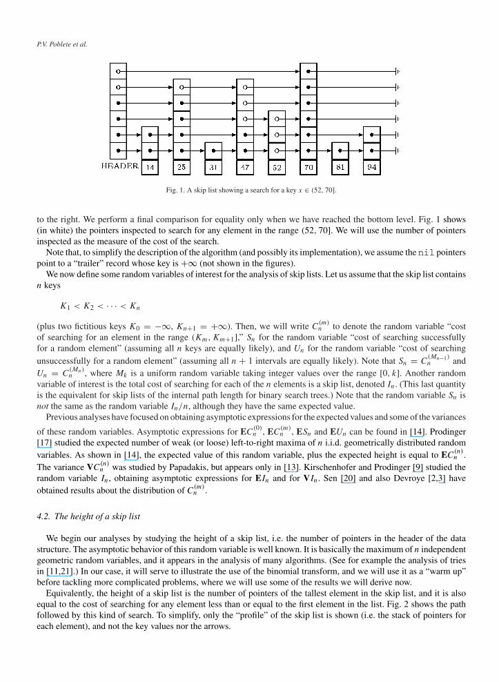
A (probabilistic) skip list [18] is a generalization of a linked list. Elements are stored in order of increasing key value,and the records are linked into several lists (see Fig. 1).

The bottom such list links all elements, and each successive list links a subset of the elements in the list below it. Foreach element in a given list, the decision to link it into the next level list is made probabilistically: a (possibly biased)coin is flipped, and if it lands “heads” the element is included in the next level list. In our analyses we will assume thatthe coin has probability p of landing “heads,” and probability q = 1− p of landing “tails.”

To search for a given element x, we start at the header of the top list, and compare x to the key of the next record. Ifx is less than or equal to that key, we move down to the pointer one level below. If not, we advance to the next pointer

P.V. Poblete et al.

Fig. 1. A skip list showing a search for a key x ∈ (52, 70].

to the right. We perform a final comparison for equality only when we have reached the bottom level. Fig. 1 shows(in white) the pointers inspected to search for any element in the range (52, 70]. We will use the number of pointersinspected as the measure of the cost of the search.

Note that, to simplify the description of the algorithm (and possibly its implementation), we assume the nil pointerspoint to a “trailer” record whose key is +∞ (not shown in the figures).

We now define some random variables of interest for the analysis of skip lists. Let us assume that the skip list containsn keys

K1 < K2 < · · · < Kn

(plus two fictitious keys K0 = −∞, Kn+1 = +∞). Then, we will write C(m)n to denote the random variable “cost

of searching for an element in the range (Km, Km+1],” Sn for the random variable “cost of searching successfullyfor a random element” (assuming all n keys are equally likely), and Un for the random variable “cost of searchingunsuccessfully for a random element” (assuming all n + 1 intervals are equally likely). Note that Sn = C

(Mn−1)n and

Un = C(Mn)n , where Mk is a uniform random variable taking integer values over the range [0, k]. Another random

variable of interest is the total cost of searching for each of the n elements is a skip list, denoted In. (This last quantityis the equivalent for skip lists of the internal path length for binary search trees.) Note that the random variable Sn isnot the same as the random variable In/n, although they have the same expected value.

Previous analyses have focused on obtaining asymptotic expressions for the expected values and some of the variances

of these random variables. Asymptotic expressions for EC(0)n , EC

(m)n , ESn and EUn can be found in [14]. Prodinger

[17] studied the expected number of weak (or loose) left-to-right maxima of n i.i.d. geometrically distributed randomvariables. As shown in [14], the expected value of this random variable, plus the expected height is equal to EC

(n)n .

The variance VC(n)n was studied by Papadakis, but appears only in [13]. Kirschenhofer and Prodinger [9] studied the

random variable In, obtaining asymptotic expressions for EIn and for VIn. Sen [20] and also Devroye [2,3] haveobtained results about the distribution of C

(m)n .

4.2. The height of a skip list

We begin our analyses by studying the height of a skip list, i.e. the number of pointers in the header of the datastructure. The asymptotic behavior of this random variable is well known. It is basically the maximum of n independentgeometric random variables, and it appears in the analysis of many algorithms. (See for example the analysis of triesin [11,21].) In our case, it will serve to illustrate the use of the binomial transform, and we will use it as a “warm up”before tackling more complicated problems, where we will use some of the results we will derive now.

Equivalently, the height of a skip list is the number of pointers of the tallest element in the skip list, and it is alsoequal to the cost of searching for any element less than or equal to the first element in the list. Fig. 2 shows the pathfollowed by this kind of search. To simplify, only the “profile” of the skip list is shown (i.e. the stack of pointers foreach element), and not the key values nor the arrows.

P.V. Poblete et al.

Fig. 2. The height of a skip list.

Let Pn(z) be the probability generating function for the random variable “height of the skip list.” Since p is theprobability that we keep adding pointers when inserting an element, then if we remove the bottom layer of pointers theprobability that i elements will still have a nonempty stack of pointers, while j are left with no pointers is (i, j)piqj ,where i + j = n. Therefore,

Pn(z) = z∑

i,j �0i+j=n

(i, j)piqjPi(z) ∀n > 0

and P0(z) = 1.Whenever we have an equation xn = n valid for n > 0, we can extend it to cover the case n = 0 by changing it

into xn = [n > 0]n + [n = 0]x0 = [n�0]n + [n = 0](x0 − 0). Applying this rule to this equation, we get

Pn(z) = z∑

i,j �0i+j=n

(i, j)piqjPi(z)+ (1− z)[n = 0] ∀n�0.

Applying the binomial transform, we get

Ps(z) = zpsPs(z)+ (1− z)

or, equivalently

(1− zps)Ps(z) = (1− z). (7)

Note that we avoid taking the obvious step of solving this equation for Ps(z), because this would not be correct for thecase z = 1, s = 0.

Now, to compute the average and the variance we have to differentiate Eq. (7) and evaluate at z = 1. Let us introducethe notation an = P ′n(1), bn = P ′′n (1). Note that the average is given by an, and the variance by bn+an−a2

n. Observingthat Ps(1) = [s = 0] (because Pn(1) = 1), we obtain

as = [s > 0]ps − 1

and

bs = 2psas

1− ps= − 2ps

(ps − 1)2[s > 0].

Alternatively, we could have solved Eq. (7) to find Ps(z) = 1−z1−zps , but this would have been correct only for s > 0.

From this we would have obtained expressions for as and bs , that would also be valid only for s > 0 (the difference

from the correct ones being the lack of the factor “[s > 0]”). Noting that a0 = a0 = 0 and b0 = b0 = 0, we could thenuse the technique employed earlier to extend the solutions to expressions valid for all s�0.

P.V. Poblete et al.

To invert these transforms the following expansions are useful (see Appendix A for their derivations):

E1.1

ps − 1= −1

2+ 1

s ln p+ 1

ln p

∑k �=0

1

s + �k

= −1

2+ 1

ln p+ F

[0]s .

E2.ps

(ps − 1)2= 1

s2 ln2 p+ 1

ln2 p

∑k �=0

1

(s + �k)2= 1

s2 ln2 p− Ds F

[0]s

ln p,

where �k = 2�ikln p

. Using E1, we have

as =(−1

2+ 1

s ln p

)[s > 0] + F [0]s

and applying the inverse transform we find the following (exact) expression for the expected height of a skip list forall n�0:

an = − Hn

ln p+ 1

2 [n > 0] + F [0]n .

Let us look now at the variance. Using E2, we have that

bs =(− 2

s2 ln2 p+ 2

ln pDs F

[0]s

)[s > 0] = − 2

s2 ln2 p[s > 0] + 2

ln pDs F

[0]s −

1

6[s = 0].

Applying the inverse transform, we have that, for n�0,

bn = H 2n +H

(2)n

ln2 p− 1

6− 2

ln pF [0]n Hn + 2G[0]n .

Using this, and after some simplification, we obtain the following result:

Theorem 1. The expected value of the height of a skip list is

EC(0)n =−

Hn

ln p+ 1

2[n > 0] + F [0]n for all n�0

= log1/p n+ 1

2− �

ln p+ �(log n)+ O

(1

n

),

and its variance is equal to

VC(0)n =

H(2)n

ln2 p+ 1

12− 1

4[n = 0] − (F [0]n )2 + 2G[0]n for all n�0

= �2

6 ln2 p+ 1

12+ �(log n)+ �(log n)2 + O

(1

n

).

Note that the �(log n)2 term has a nonzero mean value. We do not have a closed form for it, but for usual values of p

its contribution is negligible (e.g., 10−11 for p = 12 ).

4.3. Searching for +∞

Let us now turn our attention to the opposite end of the data structure. A search for “+∞” is (on the average) themost expensive one. We analyze now the cost of that search.

We will use the same notation as before, but the random variable we are studying is “number of pointers inspectedwhen searching for +∞.” (We redefine Pn, an and bn accordingly.) Fig. 3 shows the path followed in this case.

Consider the search path from right to left. At the rightmost end, there is some number, say k, of elements of height 1,all of whose bottom-level pointers had to be traversed during the search. In addition, the bottom-level pointer belongingto the element immediately preceding them was also traversed. Note that this last element must be of height > 1. If we

P.V. Poblete et al.

Fig. 3. Searching for +∞ in a skip list.

now erase the bottom layer of pointers, all k rightmost elements will disappear. Of the other n− k elements, some ofthem, say i, were of height > 1, and the remaining ones, say j , were of height 1, so the latter also disappear. These i andj elements may be intermixed in any of (i − 1, j) possible orders, because one of the i “tall” elements is constrainedto be in the rightmost position.

Therefore, the generating function for the search cost is

Pn(z) = ∑i,j,k �0

i+j+k=n

(i − 1, j)piqj+kPi(z)zk+1 ∀n > 0. (8)

Note that our previous argument assumes that there is at least one element of height > 1 (i.e. i > 0), but it is easy toverify that the equation we obtained holds also for the case i = 0 (which implies j = 0, k = n).

The boundary condition is P0(z) = 1 and, as before, we can fix the equation to hold for all n�0 by adding toEq. (8) the term (1− z)[n = 0].

After the substitution h = i − 1+ j , we can obtain the following somewhat simpler form:

Pn(z) = ∑0� i �n

piqn−iPi(z)gi,n(z)+ (1− z)[n = 0] ∀n�0, (9)

where

gi,n(z) = ∑i−1�h�n−1

(h

i − 1

)zn−h.

The summation defining the function gi,n(z) does not seem to have a simple closed form, but its derivatives at z = 1are not hard to find. It can be shown by induction that

gi,n(1)=(

n

i

),

g(k)i,n (1)= k!

(n+ 1

i + k

)∀k�1.

Differentiating Eq. (9) to find the average an = P ′n(1), we get

an = ∑0� i �n

piqn−i

((n

i

)ai +

(n+ 1

i + 1

))− [n = 0]

= ∑0� i �n

(n

i

)piqn−iai + 1− qn+1

p− [n = 0].

Note that this equation holds for all n�0, but in itself does not determine a unique value for a0. Therefore, we willhave to handle the boundary condition a0 = 0 separately. Applying the transform and using rule R8, we have

as = psas + [s = 0]p− qps−1 − 1.

P.V. Poblete et al.

Again, this equation holds for s = 0, but it does not determine a0. To work around this problem, we will solve theequation for s �= 0, getting

as = q

p+ 1

p(ps − 1)

and then fix it to incorporate the boundary condition. The resulting solution is

as =(

q

p+ 1

p(ps − 1)

)[s > 0]

= [s > 0]sp ln p

+(

1

2p− 1

)[s > 0] + F

[0]s

p. (10)

Applying the inverse transform, we find that the expected cost of searching for +∞ is

an = − Hn

p ln p+(

1− 1

2p

)[n > 0] + F

[0]n

p

for all n�0.To find the variance, we differentiate Eq. (9) twice and set z = 1, obtaining

bn = ∑0� i �n

piqn−i

((n

i

)bi + 2

(n+ 1

i + 1

)ai + 2

(n+ 1

i + 2

))

= ∑0� i �n

(n

i

)piqn−ibi + 2

∑0� i �n

(n+ 1

i + 1

)piqn−iai + 2q

p2(1− qn − npqn)

with b0 = 0.Applying the binomial transform and using rules R8 and R10, we get

bs = psbs + 2psas − 2ps−1q∑

0� t<s

at + 2q

p2[s = 0] − 2qps−2 + 2sq2ps−2.

Solving this first for s > 0, and then introducing the boundary condition b0 = 0, we obtain

bs =(− 2ps

p2(ps − 1)2+ 2qps

p2(ps − 1)

∑1� t � s

1

pt − 1

)[s > 0]. (11)

The summation can be expanded as follows:

∑1� t � s

1

pt − 1=− ∑

1� t � s

(1+ ∑

k �1pkt

)

=−s − ∑k �1

pk(1− pks)

1− pk

=−s − ∑k �1

1− pks

p−k − 1.

Replacing this in (11), we get

bs =(− 2ps

p2(ps − 1)2− 2qsps

p2(ps − 1)− 2q

p2

∑k �1

ps(1− pks)

(ps − 1)(p−k − 1)

)[s > 0]

=(− 2ps

p2(ps − 1)2− 2qs

p2

(1+ 1

ps − 1

)− 2q

p2

∑k �1

ps(1− pks)

(ps − 1)(p−k − 1)

)[s > 0].

Note that

ps(1− pks)

ps − 1= −(ps + p2s + · · · + pks) = −k + ∑

1� j �k

(1− pjs).

P.V. Poblete et al.

Therefore,

bs =(− 2ps

p2(ps − 1)2− 2qs

p2

(1+ 1

ps − 1

)+ 2q

p2

∑k �1

k

p−k − 1− 2q

p2

∑1� j �k

1− pjs

p−k − 1

)[s > 0].

We are almost ready to apply the inverse transform to this function. The first two terms have known expansions, and thesummation in the third term is convergent. We will denote �(p) =∑k �1

kp−k−1

(for instance, �( 12 ) ≈ 2.744 . . .). We

will consider the fourth term in more detail later. For the time being, let us denote ds = −∑1� j �k (1−pjs)/(p−k−1)

(note that this is a double summation).Using our known expansions, we have that

bs =(− 2

p2

(1

s2 ln2 p− Ds F

[0]s

ln p

)− 2q

p2

(s

2+ 1

ln p+ sF [0]s

)+ 2q

p2�(p)+ 2q

p2ds

)[s > 0],

whose inverse transform is

bn =(

H 2n +H

(2)n

p2 ln2 p− 1

6p2− 2F

[0]n Hn

p2 ln p+ 2

p2G[0]n

+ q

p2[n = 1] + 2q

p2 ln p+ 2q

p2F [1]n −

2q

p2�(p)+ 2q

p2dn

)[n > 0].

Before stating our results for this section, we need to study the behavior of the function dn, whose transform is definedby the double summation

ds = − ∑1� j �k

1− pjs

p−k − 1.

Applying the inverse transform, we have that

dn = − ∑1� j �k

[n = 0] − (1− pj )n

p−k − 1= ∑

1� j �k

(1− pj )n

p−k − 1[n > 0].

Clearly, this function is always nonnegative for p < 1. For an upper bound, observe that p�1 implies that p−j −1�p(p−(j+1) − 1), and this in turn implies that 1

p−(j+1)−1� p

p−j−1. Therefore, 1

p−(j+k)−1� pk

p−j−1and

∑k � j

1

p−k − 1= ∑

k �0

1

p−(j+k) − 1� 1

p−j − 1

∑k �0

pk = pj

q(1− pj )

and

dn � 1

q

∑j �1

pj (1− pj )n−1[n > 0] = 1

q

∑j �1

((1− pj )n−1 − (1− pj )n).

To finish computing this bound, we now go back to the transformed domain. Since rule R7 allows us to find thetransform of functions of the form n(an − an−1), it turns out to be simpler to bound ndn rather than dn. We have that

Bs

∑j �1

n((1− pj )n−1 − (1− pj )n

)= −s

∑j �1

pjs[s > 0] = sps

ps − 1[s > 0].

Inverting this transform, we get

ndn � 1

q

(−1

2[n = 1] − 1

ln p− F [1]n

)[n > 0]

and therefore dn = O( 1n).

P.V. Poblete et al.

The following theorem summarizes the results obtained in this section:

Theorem 2. The expected value of the cost of searching for +∞ in a skip list is

EC(n)n =−

Hn

p ln p+(

1− 1

2p

)[n > 0] + F

[0]n

pfor all n�0

= 1

plog1/p n+ 1− 1

2p− �

p ln p+ �(log n)+ O

(1

n

)

and its variance is

VC(n)n =−

q

p2 ln pHn + q

p2[n = 1] +

(H

(2)n

p2 ln2 p+ 1

2p− 5

12p2+ 2q

p2 ln p− 2q

p2�(p)

+ q

p2F [0]n −

(F[0]n )2

p2+ 2q

p2F [1]n +

2

p2G[0]n +

2q

p2dn

)[n > 0] for all n�0

= q

p2log1/p n

+ �2

6p2 ln2 p+ 1

2p− 5

12p2+ q(2− �)

p2 ln p− 2q

p2�(p)

+ �(log n)+ �(log n)2 + O

(1

n

)as n→∞,

where �(p) =∑k �1k

p−k−1.

4.4. Searching for an arbitrary element

We consider now a more general case. Suppose the element we are looking for is not necessarily the first or the lastone in the list, but an arbitrary one (see Fig. 4). If we assume that the rank of the element is known to us, we can viewthe list as partitioned in two sections: the left part, of size n1 contains all elements smaller than the given one; the rightpart, of size n2, contains all elements greater than or equal to the given one. (Of course, n1 + n2 = n.)

Generalizing our notation, we write Pn1,n2(z) for the probability generating function of the search cost. In a similarway, we write an1,n2 and bn1,n2 .

Note that we have already studied the cases n1 = 0 (height of the skip list, or cost of searching for the first element)and n2 = 0 (cost of searching for +∞). Also note that this means that we already know the results for the case s1 = 0and for the case s2 = 0 in the transformed domain.

The recurrence equation for Pn1,n2(z) is

Pn1,n2(z) =∑

i,j,k,�,m�0i+j+k=n1�+m=n2

(i − 1, j)piqj+kzk+1(�, m)p�qmPi,�(z)+ (1− z)[n1 = 0][n2 = 0]

with P0,0(z) = 1.This can be rewritten as

Pn1,n2(z) =∑

0� i �n10���n2

piqn1−igi,n1(z)

(n2

�

)p�qn2−�Pi,�(z)+ (1− z)[n1 = 0][n2 = 0].

Applying a binomial transform to n2, we get

Pn1,s2(z) = ps2∑

0� i �n1

piqn1−igi,n1(z)Pi,s2(z)+ (1− z)[n1 = 0][s2 �0].

P.V. Poblete et al.

Fig. 4. Searching for an arbitrary element.

It does not seem possible to simplify this further, so we differentiate this equation to obtain equations for the moments:

an1,s2 = ps2

( ∑0� i �n1

(n1

i

)piqn1−i ai,s2 +

1− qn1+1

p[s2 = 0]

)− [n1 = 0][s2 �0].

We now apply the transform to n1, using rule R8 to obtain

as1,s2 = ps1+s2 as1,s2 +1

p[s1 = 0][s2 = 0] − q

pps1 [s2 = 0] − [s1 �0][s2 �0].

We solve this equation first assuming s1 + s2 > 0, and then introducing the boundary condition a0,0 = 0. The result is

as1,s2 =q

p

(1+ 1

ps1 − 1

)[s1 > 0][s2 = 0] + 1

ps1+s2 − 1[s1 + s2 > 0].

This expression resembles the one we found for as when studying the problem of searching for +∞ (Eq. (10)). In ourcurrent notation, Eq. (10) can be rewritten as

as,0 =(

q

p+ 1

p(ps − 1)

)[s > 0].

Using this connection with our earlier results, we can rewrite as1,s2 as follows:

as1,s2 = qas1,0[s2 = 0] + pas1+s2,0 − q[s1 �0][s2 > 0]and computing its inverse (using property P1) we find that the average search cost is

an1,n2 = qan1,0 + pan1+n2,0 + q[n1 = 0][n2 > 0]=(−Hn1+n2

ln p+ 1

2+ F

[0]n1+n2

)[n1 + n2 > 0] + q

p

(−Hn1

ln p− 1

2+ F [0]n1

)[n1 > 0]

for n1, n2 �0.Let us look now at the variance. We have

bn1,s2 = ps2∑

0� i �n1

piqn1−i

((n1

i

)bi,s2 + 2

(n1 + 1

i + 1

)ai,s2 + 2

(n1 + 1

i + 2

)[s2 = 0]

)

= ps2∑

0� i �n1

(n1

i

)piqn1−i bi,s2 + 2ps2

∑0� i �n1

(n1 + 1

i + 1

)piqn1−i ai,s2

+ 2q

p2(1− qn1 − n1pqn1)[s2 = 0]

P.V. Poblete et al.

with b0,0 = 0. Applying the transform to n1, we get

bs1,s2 = ps1+s2 bs1,s2 + 2ps1+s2 as1,s2 − 2qps1+s2−1 ∑0� t<s1

at,s2

+(

2q

p2[s1 = 0] − 2qps1−2 + 2s1q

2ps1−2)[s2 = 0].

Solving this equation, we obtain

bs1,s2 =−2q

p

ps1

(ps1 − 1)2[s1 > 0][s2 = 0] + 2q2

p2

ps1

ps1 − 1

∑1� t<s1

1

pt − 1[s2 = 0][s1 > 0]

− 2ps1+s2

(ps1+s2 − 1)2[s1 + s2 > 0] + 2q

p

ps1+s2

ps1+s2 − 1

∑s2 � t<s1+s2

1

pt − 1[t > 0][s1 + s2 > 0].

As we did for as1,s2 , this can be expressed in terms of bs,0 from (11). In terms of this function, bs1,s2 can be expressedas follows:

bs1,s2 = qbs1,0[s2 = 0] + pbs1+s2,0 −2q

p

ps1+s2

ps1+s2 − 1

∑1� t<s2

1

pt − 1[s1 + s2 > 0].

From this expression, we can obtain an explicit formula for bn1,n2 (and therefore for the variance) using the definitionof the inverse transform, but we have been unable to find a closed form. In spite of this, the expression we have foundhere for bs1,s2 will enable us in the next section to find the variance of the cost of searching for a random element.

Therefore, we state only our results for the expected cost:

Theorem 3. The expected cost of searching for an element in the range (Km, Km+1] in a skip list is

EC(m)n =

(− Hn

ln p+ 1

2+ F [0]n

)[n > 0] + q

p

(−Hm

ln p− 1

2+ F [0]m

)[m > 0] for all 0�m�n

= log1/p n+ q

plog1/p m+ 1− 1

2p− �

p ln p+ �(log n)+ �(log m)+ O

(1

m

)+ O

(1

n

)as m, n→∞.

4.5. Searching for a random element

We consider the case of an unsuccessful search for a random element. When the search stops, the list has been splitin (n1, n2) elements as in the previous section, and the n+ 1 possible splits are equally likely.

If we write Pn(z) to denote the probability generating function for the search cost, we have that

Pn(z) = 1

n+ 1

∑0�k �n

Pk,n−k(z)

where the P in the right-hand side is from the previous section. Using property P2 of two-dimensional binomialtransforms, we have that a similar relationship holds between their transforms:

ˆP s(z) = 1

s + 1

∑0� t � s

Pt,s−t (z).

Similar equations hold for an and bn.Using this and the results from the previous section we can analyze the cost of this search. For the average, using

(4) we get

ˆas =(

p + q

s + 1

)as,0 − qs

s + 1

=(

1

sp ln p− 1

2+ F [0]s −

q

pF [−1]

s + 1

p(s + 1)

)[s > 0],

P.V. Poblete et al.

and therefore the average cost for the unsuccessful search for a random element is

an = − Hn

p ln p+ 1− 1

2p+ q

p ln p− 1

2[n = 0] + F [0]n −

q

pF [−1]

n + 1

p(n+ 1).

Consider now the variance. We have

ˆbs = 1

s + 1

∑0� t � s

bt,s−t

= 1

s + 1

∑0� t � s

(qbt,0[s − t = 0] + pbs,0 − 2q

p

ps

ps − 1

∑1� r<s−t

1

pr − 1[s > 0]

)

=(

p + q

s + 1

)bs,0 − 2q

p

ps

ps − 1

1

s + 1

∑1� r � s

s − r

pr − 1[s > 0],

where

bs,0 =(− 2

p2

ps

(ps − 1)2+ 2q

p2

ps

ps − 1

∑1� r � s

1

pr − 1

)[s > 0].

Replacing this in the previous expression and simplifying, we get

ˆbs =(− 2

p2

(p + q

s + 1

)ps

(ps − 1)2+ 2q

p2

1

s + 1

ps

ps − 1

∑1� r � s

1+ pr

pr − 1

)[s > 0].

We use now the expansion 1pr−1 = −1−∑k �1 pkr , obtaining

ˆbs =(− 2

p2

(p + q

s + 1

)ps

(ps − 1)2+(− q

ps + 2q

p2(p�(p)− 1)

(1− 1

s + 1

))ps

ps − 1

−2q

p2

ps

ps − 1

(p∑

k �1

1− pks

p−k − 1+ 1

s + 1

∑k �1

1− pks

p−k − 1+ p

s + 1

∑k �1

1− pks

(p−k − 1)2

))[s > 0],

where �(p) =∑k �11

p−k−1. Now we substitute ps

ps−1 (1− pks) = −k +∑1� j �k (1− pjs), to obtain

ˆbs =(− 2

p2

(p + q

s + 1

)ps

(ps − 1)2+(− q

ps + 2q

p2(p�(p)− 1)

(1− 1

s + 1

))ps

ps − 1

+ 2q

p2

(p�(p)+ �(p)+ p�(p)

s + 1

)+ 2q

p2(pds + es + pfs)

)[s > 0],

where �(p) = ∑k �1

kp−k−1

, �(p) = ∑k �1

k

(p−k−1)2 , ds = −∑1� j �k1−pjs

p−k−1, es = − 1

s+1

∑1� j �k

1−pjs

p−k−1, and

fs = − 1s+1

∑1� j �k

1−pjs

(p−k−1)2 .

We can now use our known expansions to get ˆbs in a form suitable for inverting the transform, and from it we canobtain bn. The resulting expressions are quite lengthy, so we will omit them and state our final results in the followingtheorem:

Theorem 4. The expected value of the cost of an unsuccessful search in a skip list is

EUn =− Hn

p ln p+ 1− 1

2p+ q

p ln p− 1

2[n = 0] + F [0]n −

q

pF [−1]

n + 1

p(n+ 1)for all n�0

= 1

plog1/p n+ 1− 1

2p+ q − �

p ln p+ �(log n)+ O

(1

n

)

P.V. Poblete et al.

and the variance is

VUn =− q

p2 ln pHn

+(

H(2)n

p2 ln2 p+ 1

2p− 5

12p2+ 3q

p2 ln p+ q(1+ p)

p2 ln2 p− 2q�(p)

p ln p− 2q(1+ p)�(p)

p2− 2q�(p)

p

+(

q(p − 2)

p2− 2q

p ln p+ 2q�(p)

p

)F [0]n +

(q(p − 3)

p2+ 2q2

p2 ln p+ 2q�(p)

p

)F [−1]

n

−(

F [0]n −q

pF [−1]

n

)2

+ q

pF [1]n +

2

pG[0]n −

2q

p2G[−1]

n + q

2p[n = 1]

+(

p2 − 6p + 3

qp2− 2q

p2 ln p− 2�(p)

p+ 2q�(p)

p2+ 2q�(p)

p− 2

pF [0]n +

2q

p2F [−1]

n

)1

n+ 1

+ 2

p2 ln p

Hn

n+ 1+ 2q

pdn + 2q

p2en + 2q

pfn − 1

p2(n+ 1)2

)[n > 0] for all n�0

= q

p2log1/p n

+ �2

6p2 ln2 p+ 1

2p− 5

12p2+ q(3− �)

p2 ln p+ q(1+ p)

p2 ln2 p− 2q�(p)

p ln p− 2q(1+ p)�(p)

p2− 2q�(p)

p

+ �(log n)+ �(log n)2 + O

(log n

n

)

where �(p) =∑k �11

p−k−1, �(p) =∑k �1

kp−k−1

, �(p) =∑k �1k

(p−k−1)2 .

Note that the first line in the huge expression for the variance is the leading term, that coincides with that of thevariance of the cost of searching for+∞. The second line shows the constant term, while lines 3–4 contain the oscillatingpart. We already know that dn = O( 1

n). A similar analysis shows that en = O(

log nn

) and fn = O( 1n). Therefore, the

three final lines contain terms that are either transient, or can be bounded by O(log n

n).

5. Conclusions and further work

We believe the main contribution of this paper is the development of a theory of the binomial transform, that brings itto a level comparable to that of other, better known, tools for solving recurrence equations. We have shown its usefulnessby deriving a number of results for the behavior of (probabilistic) skip lists. These results confirm previously knownasymptotic results. In one case (variance of the search cost for a random element) we have solved a problem that wasstill open. While we do not claim that this method is always better than alternative ones, there are certainly cases wherethe binomial transform should be the method of choice. Since no method is uniformly best, the availability of a newtool should enhance our chances of solving a given problem.

There are several ways in which this work can be continued. One obvious line of development is the application ofthis transform to the analysis of other problems. Some preliminary results indicate that some hashing algorithms canbe analyzed using the binomial transform. Another interesting line of research is to try to find ways of writing downthe equations in the domain of the binomial transform (the “s domain”) directly from the algorithm being analyzed,without going through the intermediate step of writing down recurrence equations. This is the approach that Flajoletand his group have been investigating for several kinds of generating functions, with great success (for instance,see [5]).

P.V. Poblete et al.

Acknowledgments

We thank Hosam Mahmoud for many illuminating discussions on the topic of this paper and related issues, and alsofor his very useful comments on a preliminary draft. We are grateful to the anonymous referees for their suggestions, thatgreatly improved the paper. One of the authors (Poblete) thanks the Department of Computer Science of the Universityof Waterloo, for hosting him during a sabbatical year, when this work began. A preliminary version of this paper waspresented at the Third Annual European Symposium on Algorithms, Corfu, Greece, 1995 [16].

Appendix A

A.1. Rules for the manipulation of binomial transforms

R1. Bs(�an + �bn) = �Bsan + �Bsbn.

Proof. Direct from the definition. �

R2. Bsan+1n+1 = − as+1

s+1 .

Proof. Bsan+1n+1 =

∑n (−1)n

(sn

) an+1n+1 =

∑n (−1)n 1

s+1

(s+1n+1

)an+1 = − as+1

s+1 . �

R3. Bs

∑0�k<n ak = −as−1.

Proof. Define the operator San = ∑0�k<n ak . This operator satisfies �S ≡ I. In terms of these operators, we haveBsS ≡ −Z(−�)s−1 ≡ −Bs−1.

Bs

∑0�k �n

ak = as − as−1.

Proof. Bs(I+ S) ≡ Bs − Bs−1.

Bsan−1 = − ∑0� t<s

at Bs(an − an−1) = ∑0� t � s

at .

Proof. These are mirror images of the two previous formulas. �

R4. Bs1

n+1

∑0�k �n ak = as

s+1 .

Proof. Direct from rules R3 and R2 above.

Bs

an

n+ 1= 1

s + 1

∑0� t � s

at .

Proof. This is the mirror image of the previous formula. �

R5. Bs(an+1 − an) = −as+1.

Proof. Bs� ≡ −Z(−�)s+1 ≡ −Bs+1.

Bsan+1 = as − as+1.

Proof. This is the mirror image of the previous formula. �

R6. Bsnkan−k = (−1)kskas−k .

P.V. Poblete et al.

Proof. Bsnkan−k =∑n�k (−1)n

(sn

)nkan−k = (−1)ksk

∑n�k (−1)n−k

(s−kn−k

)an−k. �

R7. Bsnan = s(as − as−1).

Proof. Bsnan = BsEnan−1 − Bsan = (−sas−1 + (s + 1)as)− as .

Bsn(an − an−1) = sas .

Proof. This is the mirror image of the previous formula. �

R8. Bs

∑k (

nk)pkqn−kak = psas .

Proof.∑

n,k (−1)n(sn

)(nk

)pkqn−kak =∑k (−1)k

(sk

)akp

k∑

n (−1)n−k(s−kn−k

)qn−k = psas . �

R9. Bs

∑k (

nk)pkqn−kakbn−k =∑k (

sk) pkqs−kakbs−k .

Proof.∑

n,k (−1)n(sn

)(nk

)pkqn−kakbn−k =∑k

(sk

)pkak(−1)k

∑n

(s−kn−k

)(−1)n−kqn−kbn−k . But the inner summation

is just Bs−kqnbn, and we can write it as a convolution using the mirror image of rule R8 so the whole summation can

be rewritten as∑

k,j (−1)k(sk

)(s−kj

)ps−j qj akbj =∑j

(sj

)ps−j qj bj

∑k

(s−jk

)(−1)kak , and now the inner summation

is equal to as−j . The result follows by making the change of variable k = s − j . �

R10. Bs

∑k

(n+1k+1

)pkqn−kak = psas − ps−1q

∑0� t<s at .

Proof. Bs

∑k

(n+1k+1

)pkqn−kak = Bs

∑k

((nk

)+ ( nk+1

))pkqn−kak = psBs(an + q

pan−1). �

R11. Bs(an − a0) = Bs(an − a0)[n > 0] = as[s > 0].

Proof. as[s > 0] = as − a0[s = 0] = as − a0[s = 0] = Bs(an − a0) = Bs(an − a0)[n > 0]. �

A.2. Table of transforms

T1. 1 ⇀↽ [n = 0].

Proof. Bs[n�0] =∑n�0 (−1)n(sn) = [s = 0]. �

T2. [n > 0]⇀↽ −[n > 0].

Proof. Bs[n > 0] = Bs([n�0] − [n = 0]) = [s = 0] − [s�0] = −[s > 0]. �

T3. pn ⇀↽ qn.

Proof. Bspn =∑n(−1)n(

sn)pn = (1− p)s. �

T4. (nk) ⇀↽ (−1)k[n = k].

Proof. Bs(nk) = Bs(

nk)[n�0] = (−1)k(

sk)[s − k = 0]. �

T5. (nk)pn−k ⇀↽ (−1)k(

nk)qn−k .

Proof. Bs(nk)pn−k = (−1)k(

sk)(1− p)s−k. �

P.V. Poblete et al.

T6. 1n+1

⇀↽1

n+1 .

Proof. From rule R2 with an = [n > 0]. �

T7. Hn ⇀↽ −[n>0]n

.

Proof. BsHn = BsS [n�0]n+1 = −[n−1�0]

n. �

T8. 12 (H 2

n +H(2)n ) ⇀↽ −[n>0]

n2 .

Proof. From formula (6.21) of [8], Bs12 (H 2

n +H(2)n ) = BsSHn+1

n+1 = −[s>0]s2 . �

T9. 1n+x

⇀↽n!

xn+1= B(x, n+ 1).

Proof. From exercise 1.2.6–48 of [10] or formula (5.41) of [8], we have that∑

n(−1)n(sn) 1n+x= s!

xs+1. �

T10. 1(n+x)2

⇀↽ B(x, n+ 1)(�(x + n+ 1)− �(x)).

Proof. Differentiate the previous formula with respect to x. �

T11. n(Hn − 1) ⇀↽ −[n>1]n−1 .

Proof. From rule R7 and from transform T7. �

T12. Qr(m, n) ⇀↽ (−1)n(n, r) n!mn .

Proof. BsQr(m, n) = ∑n(−1)n(

sn)∑

k �0(k, r) nk

mk =∑

k �0(r+1)k

mk

∑n (−1)n(

sn)(

nk). But the inner summation is

equal to [s = k]. The result follows. �

A.3. Properties of two-dimensional binomial transforms

P1. an1,n2 = bn1+n2 ∀n1, n2 �0 ⇐⇒ as1,s2 = bs1+s2 ∀s1, s2 �0.

Proof. as1,s2 =∑

n1,n2(−1)n1+n2(

s1n1

)(s2n2

)an1,n2 =∑

n (−1)nbn

∑n1+n2=n (

s1n1

)(s2n2

). Now use Vandermonde’s con-

volution formula to replace the inner summation by(s1+s2

n

). The result follows. �

P2. bn = 1n+1

∑0�k �n ak,n−k ∀n�0 ⇐⇒ bs = 1

s+1

∑0� t � s at,s−t ∀s�0.

Proof. bs = ∑n(−1)n

n+1

(sn

)∑i+j=n ai,j = ∑i,j

(−1)i+j

i+j+1

(s

i+j

)ai,j = 1

s+1

∑i,j (−1)i+j

(s+1

i+j+1

)ai,j . Now, using formula

1.2.6–25 from [10], we replace(

s+1i+j+1

)by∑

0�k � s

(s−k

i

)(kj

). The results follows after interchanging the order of the

two summations. �

A.4. Useful expansions

E1. 1ps−1 = − 1

2 + 1s ln p+ 1

ln p

∑k �=0

1s+�k

.

Proof. We use the identities 1ps−1 = 1

2 (coth(s ln p

2 ) − 1), that follows from the definition coth x = ex+e−x

ex−e−x , and

− 12y+ �

2 coth �y =∑n�1y

n2+y2 (formula 6.3.13 in [1]), and using partial fraction decomposition. �

P.V. Poblete et al.

E2. ps

(ps−1)2 = 1s2 ln2 p

+ 1ln2 p

∑k �=0

1(s+�k)

2 .

Proof. Differentiate the previous formula with respect to s. �

References

[1] M. Abramowitz, I.A. Stegun, Handbook of Mathematical Functions, Dover, New York, 1972.[2] L. Devroye, Expected time analysis of skip lists, Technical Report, School of Computer Science, McGill University, Montreal, 1990.[3] L. Devroye, A limit theory for random skip lists, Ann. Appl. Probab. 2 (3) (1992) 597–609.[4] P. Flajolet, X. Gourdon, Ph. Dumas, Mellin transforms and asymptotics: harmonic sums, Theor. Comput. Sci. 144 (1–2) (1995) 3–58.[5] P. Flajolet, B. Salvy, P. Zimmermann, Automatic average-case analysis of algorithms, Theor. Comput. Sci. 79 (1) (1991) 37–109.[6] P. Flajolet, R. Sedgewick, Mellin transforms and asymptotics: finite differences and Rice’s integrals, Theor. Comput. Sci. 144 (1–2) (1995)

101–124.[7] G.H. Gonnet, J.I. Munro, The analysis of a linear probing sort by the use of a new mathematical transform, J. Algorithms 5 (4) (1984)

451–470.[8] R.L. Graham, D.E. Knuth, O. Patashnik, Concrete Mathematics, Addison-Wesley, Reading, MA, 1989.[9] P. Kirschenhofer, H. Prodinger, The path length of random skip lists, Acta Inform. 31 (8) (1994) 775–792.

[10] D.E. Knuth, The Art of Computer Programming, vol. 1: Fundamental Algorithms, Addison-Wesley, Reading, MA, 1997.[11] D.E. Knuth, The Art of Computer Programming, vol. 3: Sorting and Searching, Addison-Wesley, Reading, MA, 1998.[12] H. Mellin, Über den Zusammenhang zwischen den Linearen Differential- und Differenzengleichungen, Acta Math. 25 (1902) 139–164.[13] T. Papadakis, Skip lists and probabilistic analysis of algorithms, Ph.D. Thesis, University of Waterloo, Waterloo, Ontario, Canada, May 1993.

[Available as Technical Report CS-93-28.][14] T. Papadakis, J.I. Munro, P.V. Poblete, Average search and update costs in skip lists, BIT 32 (1992) 316–332.[15] P.V. Poblete, Approximating functions by their Poisson transform, Inform. Process. Lett. 23 (3) (1986) 127–130.[16] P.V. Poblete, J.I. Munro, T. Papadakis, The binomial transform and its application to the analysis of skip lists, in: Thirds Annual European

Symposium on Algorithms—ESA’95, Lecture Notes in Computer Science, vol. 979, 1995, pp. 554–569.[17] H. Prodinger, Combinatorics of geometrically distributed random variables: left-to-right maxima, Discrete Math. 153 (1996) 253–270.[18] W. Pugh, Skip lists: a probabilistic alternative to balanced trees, Comm. ACM 33 (6) (1990) 668–676.[19] J. Riordan, Combinatorial Identities, Wiley, New York, 1968.[20] S. Sen, Some observations on skip lists, Inform. Process. Lett. 39 (4) (1991) 173–176.[21] W. Szpankowski, V. Rego, Yet another application of a binomial recurrence. Order statistics, Computing 43 (1990) 401–410.