This article appeared in a journal published by Elsevier. The attachedcopy is furnished to the author for internal non-commercial researchand education use, including for instruction at the authors institution

and sharing with colleagues.

Other uses, including reproduction and distribution, or selling orlicensing copies, or posting to personal, institutional or third party

websites are prohibited.

In most cases authors are permitted to post their version of thearticle (e.g. in Word or Tex form) to their personal website orinstitutional repository. Authors requiring further information

regarding Elsevier’s archiving and manuscript policies areencouraged to visit:

http://www.elsevier.com/authorsrights

Author's personal copy

Converting pH 1:1 H2O and 1:2CaCl2 to 1:5 H2O to contribute to aharmonized global soil database☆

Zamir Libohova a,⁎, Skye Wills a, Nathan P. Odgers b, Richard Ferguson a, Rick Nesser a, James A. Thompson c,Larry T. West a, Jonathan W. Hempel a

a U.S. Department of Agriculture-Natural Resources Conservation Service, 100 Centennial Mall North, Lincoln, NE 68508, USAb The University of Sydney, Faculty of Agriculture and Environment, Biomedical Building C81, University of Sydney, New South Wales 2006, Australiac West Virginia University, Division of Plant and Soil Sciences, PO Box 6108, Morgantown, WV 26506-6108, USA

a b s t r a c ta r t i c l e i n f o

Article history:Received 28 September 2012Received in revised form 13 August 2013Accepted 16 August 2013Available online 5 October 2013

Keywords:Soil pHPedotransfer functionsGlobalSoilMap

The GlobalSoilMap initiative calls for the generation of continuous maps for soil properties, including pH in a 1:5suspension of soil in water (pH 1:5W) based on a standard method, ISO 10390. The United States Department ofAgriculture-Natural Resources Conservation Service (USDA-NRCS) employs a 1:1 suspension of soil in water(pH 1:1W), and a 1:2 suspension of soil in CaCl2 (0.01 M) (pH 1:2CaCl2) for routine pH analysis (Soil Survey Staff,2009). The objective of this study was to determine the most efficient way to convert these pH values to theGlobalSoilMap standard. For this analysis, 563 soil samples from the USDA-NRCS-National Soil Survey Center(NSSC) soil archive, which had been previously analysed for pH 1:1W and pH 1:2CaCl2, were selected for determi-nation of pH 1:5W, pH 1:5CaCl2 and electrical conductivity (EC) in 1:2 suspension of soil in water (EC 1:2W). Thesamples represented 11 soil orders, 8mineralogy classes, 5 family particle size classes, 4 geneticmaster horizons,and 7 depth intervals. For each category, 25–30 samples were selected to represent a comprehensive pH range.Regression analysis showed strong and significant relationships (R2 N 0.92) between pH methods across allcategories. The simple linear regression equation, pH 1:5W = −0.51 + 1.06 pH 1:1W, had an RMSE = 0.44pH units. Smoothing spline, did not significantly improve pH 1:5W predictions, nor did the incorporation of EC.Genetic horizons and soil depth intervals did not have a significant effect on pH 1:5W. The linear regressionmodels for predicting pH 1:5W using pH 1:1W or pH 1:2CaCl2 as predictors emerged as the best candidates for astandard pedotransfer function. Using pedotransfer functions such as these will allow for the simple conversionof existing measured and estimated pH 1:1W or pH 1:2CaCl2 values from NRCS databases to the GlobalSoilMapstandard of pH 1:5W.

Published by Elsevier B.V.

1. Introduction

Soil pH, which is an importantmeasure of soil acidity, nutrient avail-ability, and soil productivity, is considered amaster variable (Brady andWeil, 1999). Soil pH influences many biogeochemical processes in thesoil. Furthermore, pH is measured during typical analysis of soil sam-ples, and is indirectly used as a key property in soil classification systems(Soil Survey Staff, 1999). TheUSDA-NRCS Kellogg Soil Science Laborato-ry (KSSL) routinely determines pH 1:1W and/or pH 1:2CaCl2 (Miller andKissel, 2010; Soil Survey Staff, 2009). As of 2012, 300,000 samples frommore than 50,000 pedons from across the United States and around theworld have been analysed. This data is available through various portalssuch as Web Soil Survey (USDA-NRCS, 2011). These two methods areamong many different laboratory procedures used to assess soil pH in

soils around theworld, withmethods varying in the ratio of soil to solu-tion (e.g., 1:1, 1:2, 1:5) and the salt used in the solution (e.g., none, CaCl2,KCl). The GlobalSoilMap initiative calls for the generation of continuousmaps of soil pH 1:5W (pHmeasured for a ratio of 1 part soil and 5 partswater solutions) for the entire world for standard depth increments(0–5, 5–15, 15–30, 30–60, 60–100, and 100–200 cm) (GlobalSoilMap,2012).

In the absence of a single, universally-used method for determiningsoil pH, the GlobalSoilMap specifications refer to the soil science litera-ture for functions to convert between the various pH methods(GlobalSoilMap, 2012), including the work of Conyers and Davey(1988), Bruce et al. (1989), Aitken and Moody (1991), and Miller andKissel (2010) (Table 1). In most of this work, the relationships devel-oped for converting between methods were based on relatively smallor geographically-limited sample sets. For example, Bruce et al. (1989)used 182 soil samples and Aitken and Moody (1991) used 90 samplesto develop relationships for converting between pH 1:5CaCl2 andpH 1:5W for acidic soils in Australia. Conyers and Davey (1988) devel-oped relationships for converting between pH 1:5CaCl2 and pH 1:5W

Geoderma 213 (2014) 544–550

☆ For inquiring about the data used in this article, please check webmaster@lin.usda.gov.⁎ Corresponding author.

0016-7061/$ – see front matter. Published by Elsevier B.V.http://dx.doi.org/10.1016/j.geoderma.2013.08.019

Contents lists available at ScienceDirect

Geoderma

j ourna l homepage: www.e lsev ie r .com/ locate /geoderma

Author's personal copy

based on 11 soil samples from Australia. Miller and Kissel (2010)analysed 120 soil samples from 33 US states and two Canadian prov-inces and developed relationships for various methods includingpH 1:1W, pH 1:1CaCl2, pH 1:2W, pH 1:2CaCl2, and pH of saturated pasteextract. Large datasets were used for two studies relating pH 1:5W and1:5CaCl2. Ahern et al. (1995) developed relationships based on 7894soil samples and Henderson and Bui (2002) based on 70,465 soil sam-ples both from Australia. We know of no studies that have developedrelationships for converting from pH 1:1W and 1:2CaCl2 to pH 1:5W in-cluding those cited by GlobalSoilMap. While a few studies have investi-gated the influence of factors such as soil depth on pH (Bruce et al.,1989) the authors found none that evaluate the relationship of soilorder, texture and mineralogy to soil pH.

Many researchers have found that the relationship betweenpH 1:5W and pH 1:5CaCl2 is not linear across the entire range of mea-sured soil pH values (Ahern et al., 1995; Aitken and Moody, 1991;Bruce et al., 1989; Henderson and Bui, 2002). Various mechanismshave been offered in soil science literature to explain the non-linearity, such as: (i) calcium carbonate buffering for high soil pH; (ii)displacement and hydrolysis of Al3+ from exchange sites by CaCl2 forlow soil pH (Little, 1992), and (iii) variable charge theory (Aitken andMoody, 1991). Thiswork has resulted in thedevelopment of various cal-ibration equations from linear functions to higher-order polynomialsand spline functions (Ahern et al., 1995; Aitken and Moody, 1991;Bruce et al., 1989; Conyers and Davey, 1988; Henderson and Bui,2002; Little, 1992; Miller and Kissel, 2010; Minasny et al., 2011).When comparing pH 1:5W and pH 1:5CaCl2 methods, Aitken andMoody (1991) found a quadratic function to fit the data better than asimple linear regression, but Ahern et al. (1995) found that the quadrat-ic function was not suitable for a wide range of pH values. Little (1992)found a cubic function that best described the relationships for pH's b5and N7. Henderson and Bui (2002) found the smoothing spline functionwith six degrees of freedom to be a better fit for a wide range of pHvalues from 2.5 to 10.5. More recently, Minasny et al. (2011) includedelectrical conductivity (EC) in the prediction of pH1:5CaCl2 from 1:5W,which improved predictions for acid and alkaline pH values.

The National Cooperative Soil Characterization Database (SCDB)contains data on more than 50,000 soil samples (National CooperativeSoil Survey, 2011). This extensive database affords an excellent oppor-tunity to establish relationships between methods of soil pH measure-ment using soil samples that represent many soil orders, mineralogyand family particle size classes, as well as different genetic horizonsand soil depths, which have not been the case for the other studies.

The objectives of this studywere to (i) develop statistical relationshipsbetween soil pH 1:1W, 1:2CaCl2, EC and 1:5W using a variety of methods,

and to (ii) discern the influence, if any, of other categorical soil variableson those relationships. The development of these relationships will en-able the conversion of soil pH 1:1W and pH 1:2CaCl2 as routinely deter-mined by the National Soil Science Center-Kellogg Soil ScienceLaboratory (NCSS-KSSL) to the soil pH 1:5W required to meetGlobalSoilMap specifications. The selected pedotransfer functions willbe used to convert the State Soil Geographic STATSGO2 (Soil SurveyStaff, 2011a,b) database pH values to pH1:5W that will then be used togenerate predictive soil pHmaps that conform to theGlobalSoilMap spec-ifications similar to the ones produced by Odgers et al. (2012) for soil or-ganic carbon.

2. Material and methods

2.1. Soil samples

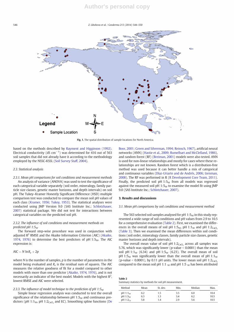
A total of 563 soil samples representing 98 pedons from the SCDB andphysically archived at the KSSL that had been previously analysed forsoil pH 1:1W and pH 1:2CaCl2 were selected for determination of soilpH 1:5W, pH 1:5CaCl2, and EC. In this paper, only the results for the con-version of soil pH 1:1W and pH 1:2 CaCl2 to pH 1:5W will be presentedalong with the influence of EC. The soil samples represented 11 soil or-ders (Alfisols, Andisols, Aridisols, Entisols, Gelisols, Histosols, Inceptisols,Mollisols, Spodosols, Ultisols, and Vertisols; Soil Survey Staff, 1999); 8mineralogy classes (Amorphic, Glassy, Glassy over amorphic, Halloysitic,Isotic, Kaolinitic, Mixed, and Smectitic; Soil Survey Staff, 2010); 5 familyparticle size classes (Clayey, Coarse loamy, Fine loamy, Fine silty, andSandy; Schoeneberger et al., 2012), 4 genetic master soil horizons(O, A, B, and C) (Soil Survey Staff, 1999); and 7 depth intervals(0–10 cm, 10–15 cm, 15–30 cm, 30–60 cm, 60–100 cm, 100–200 cm,and 200–350 cm). Each class had 25 to 30 samples that represented acomprehensive range of soil pH values from 2.9 to 10.5 and a wide geo-graphic distribution (Fig. 1). The spatial distribution of point locationsshows uneven representation of the southwestern US because thedeserts have not been sampled as intensively as the agricultural areas.However, an adequate sample size of 24 samples from Aridisols repre-sents soils of high importance for agriculture.

2.2. Analytical procedures

All soil samples had been previously analysed for pH 1:1W and1:20.01 MCaCl2 according to the methods used by the KSSL (Soil SurveyStaff, 2009). It was assumed that the likelihood of major changes inthe pH is very low for dried samples that are stored in closed containersand at room temperatures. pH1:5W and pH 1:5CaCl2 were determined

Table 1Models for relating various pH methods.

No. obs. Predicted Predictor(s) Model R2 Source

11583 pH 1:5Caa pH 1:5W, EC1:5W Linear 0.94 Minasny et al. (2011)

11583 pH 1:5Ca pH 1:5W, EC1:5W Curvilinear 0.95 Minasny et al. (2011)120 pH 1:1W pH 1:1Ca

b, EC1:1WExponential 0.99 Miller and Kissel (2010)

120 pH 1:2W pH 1:1Ca, EC1:1W Exponential 0.98 Miller and Kissel (2010)70465 pH 1:5Ca pH 1:5W Smoothing spline 0.96 Henderson and Bui (2002)7894 pH 1:5Ca pH 1:5W Linear 0.93 Ahern et al. (1995)7894 pH 1:5Ca pH 1:5W Second order polynomial 0.93 Ahern et al. (1995)7894 pH 1:5Ca pH 1:5W Third order polynomial 0.94 Ahern et al. (1995)1342 pH 1:5Ca pH 1:5W Linear 0.89 Little (1992)1342 pH 1:5Ca pH 1:5W Second order polynomial Na Little (1992)1342 pH 1:5Ca pH 1:5W Third order polynomial Na Little (1992)90 pH 1:5Ca pH 1:5W Linear 0.88 Aitken and Moody (1991)90 pH 1:5Ca pH 1:5W Second order polynomial 0.92 Aitken and Moody (1991)90 pH 1:5Ca pH 1:5W Linear 0.90 Aitken and Moody (1991)90 pH 1:5Ca pH 1:5W Second order polynomial 0.94 Aitken and Moody (1991)182 pH 1:5Ca pH 1:5W Linear 0.68 Bruce et al. (1989)11 pH 1:5Ca pH 1:5W Linear 0.99 Conyers and Davey (1988)

a pH (1:5 0.01 m CaCl2).b pH (1:1 0.01 m CaCl2).

545Z. Libohova et al. / Geoderma 213 (2014) 544–550

Author's personal copy

based on the methods described by Rayment and Higginson (1992).Electrical conductivity (dS cm−1) was determined for 416 out of 563soil samples that did not already have it according to the methodologyemployed by the NSSC-KSSL (Soil Survey Staff, 2004).

2.3. Statistical analysis

2.3.1. Mean pH comparisons for soil conditions and measurement methodsAn analysis of variance (ANOVA)was used to test the significance of

each categorical variable separately (soil order, mineralogy, family par-ticle size classes, genetic master horizons, and depth intervals) on soilpH. The Tukey–Kramer Honestly Significant Difference (HSD) multiplecomparison test was conducted to compare the mean soil pH values ofeach class (Kramer, 1956; Tukey, 1953). The statistical analyses wereconducted using JMP Version 9.0 (SAS Institute Inc.; Schlotzhauer,2007) statistical package. We did not test for interactions betweencategorical variables on the predicted soil pH.

2.3.2. The influence of soil conditions and measurement methods onpredicted pH 1:5W

The forward step-wise procedure was used in conjunction withadjusted R2 RMSE and the Akaike Information Criterion (AIC) (Akaike,1974, 1976) to determine the best predictors of pH 1:5W. The AICexpression is:

AIC ¼ N lnRe þ 2p

where N is the number of samples, p is the number of parameters in themodel being evaluated and Re is the residual sum of squares. The AICmeasures the relative goodness of fit for a model compared to othermodels with more than one predictor (Akaike, 1974, 1976), and is notnecessarily an indicator of the best model. Models with the highest R2,lowest RMSE and AIC were selected.

2.3.3. The influence of model technique to the prediction of pH 1:5WSimple linear regression analysis was conducted to test the overall

significance of the relationship between pH 1:5W and continuous pre-dictors (pH 1:1W, pH 1:2CaCl2 and EC). Smoothing spline functions (De

Boor, 2001; Green and Silverman, 1994; Reinsch, 1967), artificial neuralnetworks (ANN) (Hastie et al., 2009; Rumelhart andMcClelland, 1986),and random forest (RF) (Breiman, 2001) models were also tested. ANNis used for non-linear relationships andmostly for caseswhere these re-lationships are not known. Random forest which is a distribution-freemethod was used because it can better handle a mix of categoricaland continuous variables (Díaz-Uriarte and de Andrés, 2006; Izenman,2008). The RF was performed in R (R Development Core Team, 2011).Finally, the predicted soil pH 1:5W from all models was regressedagainst the measured soil pH 1:5W to examine the model fit using JMP9.0 (SAS Institute Inc.; Schlotzhauer, 2007).

3. Results and discussions

3.1. Mean pH comparisons by soil conditions and measurement method

The563 selected soil samples analysed for pH 1:5W in this study rep-resented a wide range of soil conditions and pH values from 2.9 to 10.5for a comprehensive evaluation (Table 2). First, we examined the differ-ences in the overall means of soil pH 1:5W, pH 1:1W and pH 1:2CaCl2(Table 3). Then we examined the mean differences within soil condi-tions (soil order, mineralogy classes, family particle size classes, geneticmaster horizons and depth intervals).

The overall mean value of soil pH 1:2CaCl2 across all samples was5.76, which was significantly lower (p-value b 0.0001) than the meansoil pH 1:1W (6.34) and pH 1:5W (6.23). The overall mean of soilpH 1:5W was significantly lower than the overall mean of pH 1:1W(p-value b 0.0001), by 0.11 pH units. The lower mean soil pH 1:2CaCl2compared to the mean soil pH 1:1 W and pH 1:5 W has been attributed

Fig. 1. The spatial distribution of sample locations for North America.

Table 2Summary statistics by methods for soil pH measurement.

Method Mean St. dev. Min. Median Max.

pH 1:1W 6.2 1.5 3.5 6.0 10.4pH 1:5W 6.3 1.3 3.4 6.2 10.5pH 1:2Ca 5.8 1.4 2.9 5.6 10.5

546 Z. Libohova et al. / Geoderma 213 (2014) 544–550

Author's personal copy

to the ionic strength of the soil solution (Aitken and Moody, 1991;Conyers and Davey, 1988; Miller and Kissel, 2010). Addition of salts tothe solution lowers the pH due to the exchange of Ca2+ with H+ andAl3+ on solid surfaces (Kissel et al., 2009; Miller and Kissel, 2010;Pierre et al., 1970; Schofield and Taylor, 1955). The lower mean of soilpH 1:5W compared to the mean of pH 1:1W has been attributed to a di-lution effect (Aitken andMoody, 1991; Conyers and Davey, 1988;Millerand Kissel, 2010). For example, Keaton (1938) and Davis (1943) foundthat increasing the water:soil ratio from 1:10 to 10:1 resulted in adecrease of 0.40 pH units.

For all methods of soil pH determination, there were significant dif-ferences between the means of the soil order, mineralogy, and familyparticle size classes; however, there were no significant differences be-tween the means of the genetic master horizons and depth intervals(Table 3). The lack of difference between depths and genetic masterhorizons is likely due to the variability of parent materials and otherfactors with depth across the dataset. Bruce et al. (1989) found thatthe pH1:5 W had the same modal range (5.0–5.5) for 91 surface andsubsurface samples from acid soil in Queensland, Australia.

Multiple-comparisons of mean pH values (results not shown) showthat the mean soil pH of Aridisols was significantly higher than themean soil pH of the other soil orders for all methods of soil pH determi-nation. Ultisols (4.61–5.27), Spodosols (4.27–4.86), and Histosols(4.83–5.69) had the lowest soil pH. The higher mean value of Aridisolsfor all pHmeasurementmethods compared to other soil orders is likelydue to the accumulation of water-soluble minerals. In environments,with a general lack of precipitation where Aridisols are typicallyfound, these more soluble minerals do not leach out of the profile,with compounds such as calcium carbonate driving higher pH values(Buol et al., 2003; Soil Survey Staff, 2010). Ultisols generally undergointense weathering and leaching of primaryminerals that contain calci-um, magnesium and potassium. This leads to relatively acidic soil pHvalues (Buol et al., 2003; Soil Survey Staff, 2010). The subsurface accu-mulation of humus–aluminiumand humus–iron complexes is partly re-sponsible for low pH values of Spodosols (Buol et al., 2003; Soil SurveyStaff, 2010), whereas Histosols found in rain-dependent raised bogscan have soil pH values that vary between 3 and 5.5 (Buol et al., 2003;Soil Survey Staff, 2010).

The overall mean soil pH of the smectitic soils was significantlyhigher than that of the other mineralogy classes for all methods of soilpH determination. The mean pH values were 7.19 for pH 1:2CaCl2 to7.81 for pH 1:5W. The overall mean soil pH of clayey soils was signifi-cantly higher than the overall mean soil pH of soils in the other familyparticle size classes, for all methods of soil pH determination. Themean pH values were 6.29 for pH 1:2CaCl2 and 6.91 for pH 1:5W. Thehigher pH values for Vertisols have been linked to their predominatelysmectitic mineralogy and finer soil texture (Chan et al., 1988; Danget al., 1994a,b; Uehara and Keng, 1974). For example, Dang et al.(1994a,b) found that the mean pH 1:5 W for 14 Vertisols soil samplesin Queensland, Australia was 8.5 (7.5–9.0) with a mean smectitic claycontent of 75% (57–91%). Chan et al. (1988) also found the meanpH 1:5 W for 9 Vertisols soil samples to be 7.8 (6.7–8.8)which is highercompared to other soil orders. For this study, 42% of the smectitic sam-ples belonged to Vertisols, which had also the highest pH values for all

pHmeasurementmethods. Also 50% of clayey soils sampleswere smec-titic which explains partly the higher pH values compared to other fam-ily particle size classes. The differences between mineralogy classescould not be explained completely by soil order or in the case of familyparticle size class bymineralogy differences. In this study, it was difficultto separate these effects.

3.2. The influence of model technique on the prediction of pH 1:5W

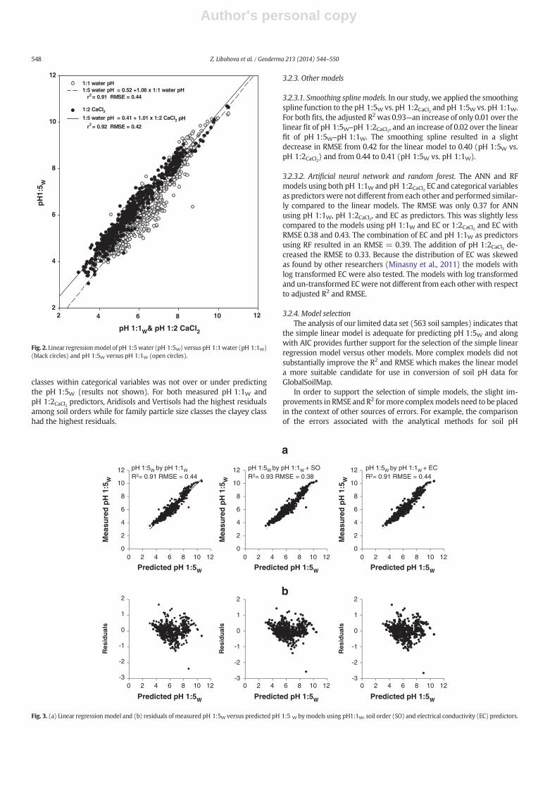
3.2.1. Linear regression modelsSimple linear regression of the pH 1:5W on pH 1:1W and pH 1:2CaCl2

revealed highly significant linear relationships (Table 4). The slope ofthe regression lines for pH 1:5W–pH 1:1W was 1.06 with an RMSE of0.44 pH units, and for pH 1:5W–pH 1:2CaCl2 was 1.01 with an RMSE of0.42 pH units. In each case, more than 90% of the variability in soilpH 1:5W was explained by pH 1:1W or pH 1:2CaCl2.

3.2.2. Multiple linear regression modelsThe AIC along with adjusted R2 and RMSE determined the statistical

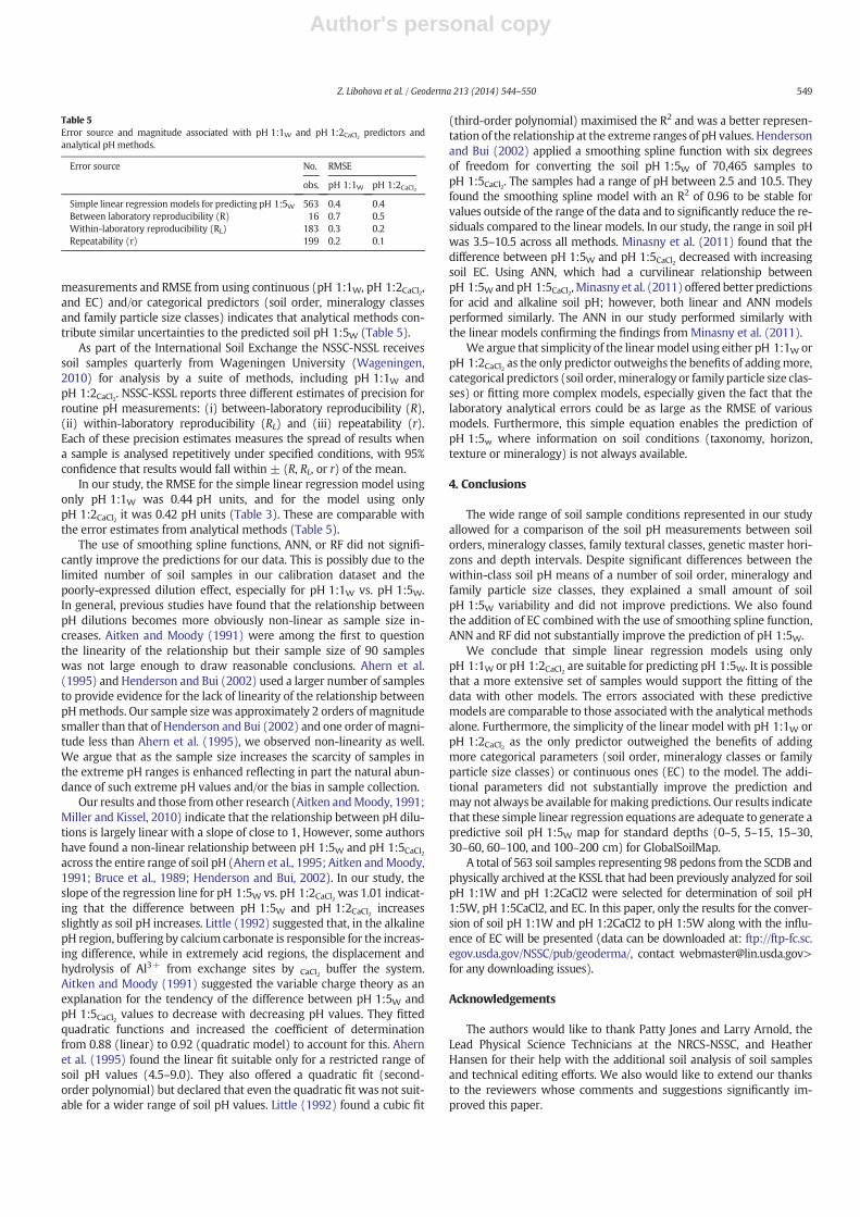
model that minimized the loss of information while keeping the num-ber of model parameters (predictors) at minimum. The “best” modelresulting from the step-wise forward procedure that included all con-tinuous and categorical variableswas the onewith pH 1:1W, pH 1:2CaCl2,soil order, mineralogy class, family particle size class, and soil depthwith adjusted R2 0.95 and RMSE 0.33. This model was a slight improve-ment compared to the simple linear regression model with onlypH 1:1W as a predictor with an R2 of 0.91 and RMSE of 0.44 or 1:2CaCl2with an R2 of 0.92 and RMSE of 0.42 (Fig. 2). The addition of EC(Fig. 3a) as a predictor did not improve the prediction at all. Thedecrease of the AIC by the addition of categorical variables to pH 1:5Wvs. pH 1:1W and pH 1:5W pH 1:2CaCl2 models was highly variable. Thelargest decrease in AIC was observed for mineralogy class (192,pH 1:1W) followed by soil order (184, pH 1:1W). However, for themin-eralogy classwhichwas the best case scenario the adjusted R2 increasedby only 0.03 while RMSE decreased by only 0.07 pH units.

Overall, our results indicate that categorical variables did notsubstantially improve predictions over linear regression with other pHmeasures. Ahern et al. (1995) found similar results when comparingthe influence of surface (0–0.1 m), subsurface (0.1–0.2 m; 0.2–0.3 m)and subsoil (N0.3 m) depth categories on the relationship betweenpH 1:5W and pHCaCl2. The distribution of the residual errors between

Table 3Analysis of variance (ANOVA) for the significance of classes and/or grouped mean pHvalues within each soil condition.

pH 1:5W pH 1:1W pH 1:2CaCl2

Soil conditions F ratio Prob N F F ratio Prob N F F ratio Prob N F

Soil order 37.88 b0.0001 38.89 b0.0001 32.07 b0.0001Mineralogy class 28.03 b0.0001 23.21 b0.0001 22.80 b0.0001Family particle size class 6.68 b0.0001 3.84 0.0041 4.98 0.0006Genetic master horizon 0.61 0.6000 0.94 0.4198 0.49 0.6825Depth intervals 0.63 0.7000 0.81 0.5600 0.92 0.4747

Table 4Model parameter influence on predicted pH 1:5W from the forward step-wise procedure.

Model parameters Adjusted R2 RMSE P value AIC

pH 1:1W 0.91 0.44 b0.0001 676pH 1:2CaCl2 0.92 0.42 b0.0001 621pH 1:1W & 1:2CaCl2 0.93 0.40 b0.0001 570pH 1:1W & soil order 0.94 0.37 b0.0001 489pH 1:2CaCl2 & soil order 0.95 0.35 b0.0001 441pH 1:1W & 1:2CaCl2 & soil order 0.96 0.33 b0.0001 383pH 1:1W & mineralogy class 0.94 0.39 b0.0001 484pH 1:2CaCl2 & soil mineralogy 0.94 0.38 b0.0001 473pH 1:1W & 1:2CaCl2 & mineralogy class 0.95 0.36 b0.0001 433pH 1:1W & family particle size class 0.92 0.43 b0.0001 650pH 1:2CaCl2 & family particle size class 0.93 0.41 b0.0001 596pH 1:1W & 1:2CaCl2 & family particle size class 0.94 0.38 b0.0001 526pH 1:1W & genetic master horizons 0.92 0.44 b0.0001 655pH 1:2CaCl2 & genetic master horizons 0.93 0.42 b0.0001 590pH 1:1W & 1:2CaCl2 & genetic master horizons 0.94 0.38 b0.0001 546pH 1:1W & Soil depth intervals 0.92 0.44 b0.0001 685pH 1:2CaCl2 & soil depth intervals 0.92 0.41 b0.0001 620pH 1:1 W & 1:2CaCl2 & soil depth intervals 0.93 0.40 b0.0001 572pH 1:1W & electrical conductivity 0.91 0.44 b0.0001 676pH 1:2CaCl2 & electrical conductivity 0.92 0.42 b0.0001 621pH 1:2W & 1:2CaCl2 & electrical conductivity 0.93 0.40 b0.0001 575

RMSE Root Mean Square Error.AIC Akaike Information Criterion.

547Z. Libohova et al. / Geoderma 213 (2014) 544–550

Author's personal copy

classes within categorical variables was not over or under predictingthe pH 1:5W (results not shown). For both measured pH 1:1W andpH 1:2CaCl2 predictors, Aridisols and Vertisols had the highest residualsamong soil orders while for family particle size classes the clayey classhad the highest residuals.

3.2.3. Other models

3.2.3.1. Smoothing spline models. In our study, we applied the smoothingspline function to the pH 1:5W vs. pH 1:2CaCl2 and pH 1:5W vs. pH 1:1W.For both fits, the adjusted R2 was 0.93—an increase of only 0.01 over thelinear fit of pH 1:5W–pH 1:2CaCl2, and an increase of 0.02 over the linearfit of pH 1:5W–pH 1:1W. The smoothing spline resulted in a slightdecrease in RMSE from 0.42 for the linear model to 0.40 (pH 1:5W vs.pH 1:2CaCl2) and from 0.44 to 0.41 (pH 1:5W vs. pH 1:1W).

3.2.3.2. Artificial neural network and random forest. The ANN and RFmodels using both pH 1:1W and pH 1:2CaCl2 EC and categorical variablesas predictorswere not different from each other and performed similar-ly compared to the linear models. The RMSE was only 0.37 for ANNusing pH 1:1W, pH 1:2CaCl2, and EC as predictors. This was slightly lesscompared to the models using pH 1:1W and EC or 1:2CaCl2 and EC withRMSE 0.38 and 0.43. The combination of EC and pH 1:1W as predictorsusing RF resulted in an RMSE = 0.39. The addition of pH 1:2CaCl2 de-creased the RMSE to 0.33. Because the distribution of EC was skewedas found by other researchers (Minasny et al., 2011) the models withlog transformed EC were also tested. The models with log transformedand un-transformed ECwere not different from each other with respectto adjusted R2 and RMSE.

3.2.4. Model selectionThe analysis of our limited data set (563 soil samples) indicates that

the simple linear model is adequate for predicting pH 1:5W and alongwith AIC provides further support for the selection of the simple linearregression model versus other models. More complex models did notsubstantially improve the R2 and RMSE which makes the linear modela more suitable candidate for use in conversion of soil pH data forGlobalSoilMap.

In order to support the selection of simple models, the slight im-provements in RMSE andR2 formore complexmodels need to be placedin the context of other sources of errors. For example, the comparisonof the errors associated with the analytical methods for soil pH

2 4 6 8 10 122

4

6

8

10

121:1 water pH1:5 water pH = 0.52 +1.06 x 1:1 water pH r2 = 0.91 RMSE = 0.44

1:2 CaCl21:5 water pH = 0.41 + 1.01 x 1:2 CaCl2 pH

r2 = 0.92 RMSE = 0.42

pH

1:5 W

pH 1:1W& pH 1:2 CaCl2

Fig. 2. Linear regressionmodel of pH 1:5water (pH 1:5W) versus pH 1:1water (pH 1:1W)(black circles) and pH 1:5W versus pH 1:1W (open circles).

0

2

4

6

8

10

12

Mea

sure

d p

H 1

:5W

Predicted pH 1:5W Predicted pH 1:5W Predicted pH 1:5W

Predicted pH 1:5W Predicted pH 1:5W Predicted pH 1:5W

pH 1:5W by pH 1:1W

R2= 0.91 RMSE = 0.44

0

2

4

6

8

10

12

0 2 4 6 8 10 120 2 4 6 8 10 12 0 2 4 6 8 10 12

0 2 4 6 8 10 120 2 4 6 8 10 12 0 2 4 6 8 10 12

pH 1:5W by pH 1:1W + SOR2= 0.93 RMSE = 0.38

0

2

4

6

8

10

12 pH 1:5W by pH 1:1W + ECR2= 0.91 RMSE = 0.44

Res

idu

als

Mea

sure

d p

H 1

:5W

Res

idu

als

Mea

sure

d p

H 1

:5W

Res

idu

als

-3

-2

-1

0

1

2

-3

-2

-1

0

1

2

-3

-2

-1

0

1

2b

a

Fig. 3. (a) Linear regressionmodel and (b) residuals of measured pH 1:5W versus predicted pH 1:5 W bymodels using pH1:1W, soil order (SO) and electrical conductivity (EC) predictors.

548 Z. Libohova et al. / Geoderma 213 (2014) 544–550

Author's personal copy

measurements and RMSE from using continuous (pH 1:1W, pH 1:2CaCl2,and EC) and/or categorical predictors (soil order, mineralogy classesand family particle size classes) indicates that analytical methods con-tribute similar uncertainties to the predicted soil pH 1:5W (Table 5).

As part of the International Soil Exchange the NSSC-NSSL receivessoil samples quarterly from Wageningen University (Wageningen,2010) for analysis by a suite of methods, including pH 1:1W andpH 1:2CaCl2. NSSC-KSSL reports three different estimates of precision forroutine pH measurements: (i) between-laboratory reproducibility (R),(ii) within-laboratory reproducibility (RL) and (iii) repeatability (r).Each of these precision estimates measures the spread of results whena sample is analysed repetitively under specified conditions, with 95%confidence that results would fall within ± (R, RL, or r) of the mean.

In our study, the RMSE for the simple linear regression model usingonly pH 1:1W was 0.44 pH units, and for the model using onlypH 1:2CaCl2 it was 0.42 pH units (Table 3). These are comparable withthe error estimates from analytical methods (Table 5).

The use of smoothing spline functions, ANN, or RF did not signifi-cantly improve the predictions for our data. This is possibly due to thelimited number of soil samples in our calibration dataset and thepoorly-expressed dilution effect, especially for pH 1:1W vs. pH 1:5W.In general, previous studies have found that the relationship betweenpH dilutions becomes more obviously non-linear as sample size in-creases. Aitken and Moody (1991) were among the first to questionthe linearity of the relationship but their sample size of 90 sampleswas not large enough to draw reasonable conclusions. Ahern et al.(1995) and Henderson and Bui (2002) used a larger number of samplesto provide evidence for the lack of linearity of the relationship betweenpHmethods. Our sample sizewas approximately 2 orders of magnitudesmaller than that of Henderson and Bui (2002) and one order of magni-tude less than Ahern et al. (1995), we observed non-linearity as well.We argue that as the sample size increases the scarcity of samples inthe extreme pH ranges is enhanced reflecting in part the natural abun-dance of such extreme pH values and/or the bias in sample collection.

Our results and those from other research (Aitken andMoody, 1991;Miller and Kissel, 2010) indicate that the relationship between pH dilu-tions is largely linear with a slope of close to 1, However, some authorshave found a non-linear relationship between pH 1:5W and pH 1:5CaCl2across the entire range of soil pH (Ahern et al., 1995; Aitken andMoody,1991; Bruce et al., 1989; Henderson and Bui, 2002). In our study, theslope of the regression line for pH 1:5W vs. pH 1:2CaCl2 was 1.01 indicat-ing that the difference between pH 1:5W and pH 1:2CaCl2 increasesslightly as soil pH increases. Little (1992) suggested that, in the alkalinepH region, buffering by calcium carbonate is responsible for the increas-ing difference, while in extremely acid regions, the displacement andhydrolysis of Al3+ from exchange sites by CaCl2 buffer the system.Aitken and Moody (1991) suggested the variable charge theory as anexplanation for the tendency of the difference between pH 1:5W andpH 1:5CaCl2 values to decrease with decreasing pH values. They fittedquadratic functions and increased the coefficient of determinationfrom 0.88 (linear) to 0.92 (quadratic model) to account for this. Ahernet al. (1995) found the linear fit suitable only for a restricted range ofsoil pH values (4.5–9.0). They also offered a quadratic fit (second-order polynomial) but declared that even the quadratic fit was not suit-able for a wider range of soil pH values. Little (1992) found a cubic fit

(third-order polynomial) maximised the R2 and was a better represen-tation of the relationship at the extreme ranges of pH values. Hendersonand Bui (2002) applied a smoothing spline function with six degreesof freedom for converting the soil pH 1:5W of 70,465 samples topH 1:5CaCl2. The samples had a range of pH between 2.5 and 10.5. Theyfound the smoothing spline model with an R2 of 0.96 to be stable forvalues outside of the range of the data and to significantly reduce the re-siduals compared to the linear models. In our study, the range in soil pHwas 3.5–10.5 across all methods. Minasny et al. (2011) found that thedifference between pH 1:5W and pH 1:5CaCl2 decreased with increasingsoil EC. Using ANN, which had a curvilinear relationship betweenpH 1:5W andpH 1:5CaCl2,Minasny et al. (2011) offered better predictionsfor acid and alkaline soil pH; however, both linear and ANN modelsperformed similarly. The ANN in our study performed similarly withthe linear models confirming the findings from Minasny et al. (2011).

We argue that simplicity of the linearmodel using either pH 1:1W orpH 1:2CaCl2 as the only predictor outweighs the benefits of addingmore,categorical predictors (soil order,mineralogy or family particle size clas-ses) or fitting more complex models, especially given the fact that thelaboratory analytical errors could be as large as the RMSE of variousmodels. Furthermore, this simple equation enables the prediction ofpH 1:5w where information on soil conditions (taxonomy, horizon,texture or mineralogy) is not always available.

4. Conclusions

The wide range of soil sample conditions represented in our studyallowed for a comparison of the soil pH measurements between soilorders, mineralogy classes, family textural classes, genetic master hori-zons and depth intervals. Despite significant differences between thewithin-class soil pH means of a number of soil order, mineralogy andfamily particle size classes, they explained a small amount of soilpH 1:5W variability and did not improve predictions. We also foundthe addition of EC combined with the use of smoothing spline function,ANN and RF did not substantially improve the prediction of pH 1:5W.

We conclude that simple linear regression models using onlypH 1:1W or pH 1:2CaCl2 are suitable for predicting pH 1:5W. It is possiblethat a more extensive set of samples would support the fitting of thedata with other models. The errors associated with these predictivemodels are comparable to those associated with the analytical methodsalone. Furthermore, the simplicity of the linear model with pH 1:1W orpH 1:2CaCl2 as the only predictor outweighed the benefits of addingmore categorical parameters (soil order, mineralogy classes or familyparticle size classes) or continuous ones (EC) to the model. The addi-tional parameters did not substantially improve the prediction andmay not always be available formaking predictions. Our results indicatethat these simple linear regression equations are adequate to generate apredictive soil pH 1:5W map for standard depths (0–5, 5–15, 15–30,30–60, 60–100, and 100–200 cm) for GlobalSoilMap.

A total of 563 soil samples representing 98 pedons from the SCDB andphysically archived at the KSSL that had been previously analyzed for soilpH 1:1W and pH 1:2CaCl2 were selected for determination of soil pH1:5W, pH 1:5CaCl2, and EC. In this paper, only the results for the conver-sion of soil pH 1:1W and pH 1:2CaCl2 to pH 1:5W along with the influ-ence of EC will be presented (data can be downloaded at: ftp://ftp-fc.sc.egov.usda.gov/NSSC/pub/geoderma/, contact webmaster@lin.usda.gov>for any downloading issues).

Acknowledgements

The authors would like to thank Patty Jones and Larry Arnold, theLead Physical Science Technicians at the NRCS-NSSC, and HeatherHansen for their help with the additional soil analysis of soil samplesand technical editing efforts. We also would like to extend our thanksto the reviewers whose comments and suggestions significantly im-proved this paper.

Table 5Error source and magnitude associated with pH 1:1W and pH 1:2CaCl2 predictors andanalytical pH methods.

Error source No. RMSE

obs. pH 1:1W pH 1:2CaCl2

Simple linear regressionmodels for predicting pH 1:5W 563 0.4 0.4Between laboratory reproducibility (R) 16 0.7 0.5Within-laboratory reproducibility (RL) 183 0.3 0.2Repeatability (r) 199 0.2 0.1

549Z. Libohova et al. / Geoderma 213 (2014) 544–550

Author's personal copy

References

Ahern, C.R., Baker, D.E., Aitken, R.L., 1995. Models for relating pH measurements in waterand calcium chloride for a wide range of pH, soil types and depths. Plant Soil 171,47–52.

Aitken, R.L., Moody, P.W., 1991. Interrelations between soil pH measurements in variouselectrolytes and soil solution pH in acidic soils. Aust. J. Soil Res. 29, 483–491.

Akaike, H., 1974. A new look at the statistical model identification. IEEE Trans. Autom.Control. 19 (6), 716–723. http://dx.doi.org/10.1109/TAC.1974.1100705.

Akaike, H., 1976. An information criterion (AIC). Math. Sci. 14 (153), 5–9.Brady, N.C., Weil, R.R., 1999. The Nature and Properties of Soil, 12th edition. Prentice-Hall,

Inc., New Jersey.Breiman, L., 2001. Random forests. Mach. Learn. 45 (1), 5–32.Bruce, R.C., Warrell, L.A., Bell, L.C., Edwards, D.G., 1989. Chemical attributes of some Queens-

land acid soils. I. Solid and solution phase compositions. Aust. J. Soil Res. 27, 333–351.Buol, S.W., Southhard, R.J., Graham, R.C., McDaniel, P.A., 2003. Soil Genesis and Classifica-

tion, 5th edition. Iowa State Press, Ames, Iowa.Chan, K.Y., Belloti,W.D., Roberts, W.P., 1988. Changes in surface soil properties of Vertisols

under dryland cropping in a semi-arid environment. Aust. J. Soil Res. 26, 509–518.Conyers, M.K., Davey, B.G., 1988. Observations on some routinemethods for soil pH deter-

mination. Soil Sci. 145, 29–36.Dang, Y.P., Dalal, R.C., Edwards, D.G., Tiller, K.G., 1994a. Kinetics of zinc desorption from

Vertisols. Soil Sci. Soc. Am. J. 58, 1392–1399.Dang, Y.P., Tiller, K.G., Dalal, R.C., Edwards, D.G., 1994b. Zinc speciation in soil solution of

Vertisols. Aust. J. Soil Res. 34, 369–383.Davis, L.E., 1943. Measurements of pH with the glass electrode as affected by soil mois-

ture. Soil Sci. 56, 405–422.De Boor, C., 2001. A Practical Guide to Splines, Revised edition. Springer.R Development Core Team, 2011. R: A Language and Environment for Statistical Comput-

ing. R Foundation for Statistical Computing, Vienna, Austria.Díaz-Uriarte, R., de Andrés, S.A., 2006. Gene selection and classification of microarray

data using random forest. BMC Bioinformatics 3 (7). http://dx.doi.org/10.1186/1471-2105-7-3.

GlobalSoilMap, 2012. Specifications, Version 1 GlobalSoilMap.Net Products. Release 2.2.Green, P.J., Silverman, B.W., 1994. Nonparametric Regression and Generalized Linear

Models. CRC Press.Hastie, T., Tibshirani, R., Friedman, J., 2009. The Elements of Statistical Learning: Data Min-

ing, Inference and Prediction, Springer Series in Statistics, 2nd ed. Springer-Verlag,New York.

Henderson, B.L., Bui, E.N., 2002. An improved calibration curve between soil pHmeasuredin water and CaCl2. Aust. J. Soil Res. 40, 1399–1405.

Izenman, A.J., 2008. Modern Multivariate Statistical Techniques Regression, Classficationand Maniforl Learning. Springer Series in Statistics, New York.

Keaton, C.M., 1938. A theory explaining the relation of soil–water ratios to pH values. SoilSci. 46, 259–265.

Kissel, D.E., Sonon, L., Vendrell, P.F., Isaac, R.A., 2009. Salt concentration and measurementof soil pH. Commun. Soil Sci. Plant Anal. 40, 179–187.

Kramer, C.Y., 1956. Extension of multiple range tests to group means with unequal num-ber of replications. Biometrics 12, 307–310.

Little, I.P., 1992. The relationship between soil pH measurements in calcium chloride andwater suspensions. Aust. J. Soil Res. 307, 587–592.

Miller, R.O., Kissel, D.E., 2010. Comparison of soil pH methods on soils of North America.Soil Sci. Soc. Am. J. 74, 310–316.

Minasny, B., McBratney, A.B., Brough, D.M., Jacquier, D., 2011. Models relating soil pHmeasurements in water and calcium chloride that incorporate electrolyte concentra-tion. Eur. J. Soil Sci. http://dx.doi.org/10.1111/j.1365-2389.2011.01386.x.

National Cooperative Soil Survey, 2011. National Cooperative Soil Characterization Database.Available online at http://ncsslabdatamart.sc.egov.usda.gov (Accessed [July 2011]).

Odgers, N.P., Libohova, Z., Thompson, J.A., 2012. Equal-area spline functions applied to a leg-acy soil database to create weighted-means maps of soil organic carbon at a continentalscale. Geoderma 189–190, 153–163. http://dx.doi.org/10.1016/j.geoderma.2012.05.026.

Pierre, W.H., Meisinger, J., Birchett, J.R., 1970. Cation–anion balance in crops as a factor indetermining the effect of nitrogen fertilizer on soil acidity. Agron. J. 62, 106–112.

Rayment, G.E., Higginson, F.R., 1992. Australian laboratory handbook of soil and waterchemical methods. Australian Soil and Land Survey Handbook, vol. 3. Inkata Press,Melbourne.

Reinsch, Ch.H., 1967. Smoothing by spline functions. Numer. Math. 10, 177–183.Rumelhart, D., McClelland, J., 1986. Parallel Distributed Processing. MIT Press, Cambridge,

Mass.Schlotzhauer, S.D., 2007. Elementary Statistics Using JMP. SAS Institute Inc., Cary, NC.Schoeneberger, P.J., Wysocki, D.A., Benham, E.C., Soil Survey Staff, 2012. Field Book for

Describing and Sampling Soils, Version 3.0. Natural Resources Conservation Service,National Soil Survey Center, Lincoln, NE.

Schofield, R.K., Taylor, A.W., 1955. The measurement of soil pH. Soil Sci. Soc. Am. Proc. 19,164–167.

Soil Survey Staff, 1999. Soil Taxonomy, A Basic System of Soil Classification for Makingand Interpreting Soil Surveys, 2nd edition.

Soil Survey Staff, 2004. Soil Survey Laboratory MethodsManual. In: Burt, R. (Ed.), Soil Sur-vey Investigations Report No. 42, Version 4.0. U.S. Department of Agriculture, NaturalResources Conservation Service.

Soil Survey Staff, 2009. Soil Survey Field and Laboratory Methods Manual. In: Burt, R.(Ed.), Soil Survey Investigations Report No. 51, Version 1.0. U.S. Department of Agri-culture, Natural Resources Conservation Service.

Soil Survey Staff, 2010. Keys to Soil Taxonomy, 11th edition. U.S. Department of Agricul-ture, Natural Resources Conservation Service, Washington, D.C.

Soil Survey Staff, 2011a. Natural Resources Conservation Service, United StatesDepartment of Agriculture. Soil Survey Geographic (SSURGO) Database. (http://sdmdataaccess.nrcs.usda.gov/. [Accessed Dec 2011]).

Soil Survey Staff, 2011b. Natural Resources Conservation Service, United States Depart-ment of Agriculture. Web Soil Survey. (Available online at http://websoilsurvey.nrcs.usda.gov/. [Accessed Aug 2011]).

Tukey, J.W., 1953. Some selected quick and easy methods of statistical analysis. Trans. N.Y. Acad. Sci. 16 (2), 88–97.

Uehara, G., Keng, J.Ch., 1974. Management implications of soil mineralogy in LatinAmerica. Presented at Symposium on Management of Tropical Soils, Cali, Columbia(21 pp.).

United States Department of Agriculture, Natural Resources Conservation Service, 2011.National Cooperative Soil Survey, National Cooperative Soil Characterization Data-base. Available online at http://ncsslabdatamart.sc.egov.usda.gov (Accessed on Janu-ary 2011).

Wageningen, 2010. Evaluating Programs for Analytical Laboratories International Soil An-alytical Exchange Quarterly Reports. 1–4.

550 Z. Libohova et al. / Geoderma 213 (2014) 544–550