This article appeared in a journal published by Elsevier. The attachedcopy is furnished to the author for internal non-commercial researchand education use, including for instruction at the authors institution

and sharing with colleagues.

Other uses, including reproduction and distribution, or selling orlicensing copies, or posting to personal, institutional or third party

websites are prohibited.

In most cases authors are permitted to post their version of thearticle (e.g. in Word or Tex form) to their personal website orinstitutional repository. Authors requiring further information

regarding Elsevier’s archiving and manuscript policies areencouraged to visit:

http://www.elsevier.com/copyright

Author's personal copy

The crucial relationship among energy commodity prices: Evidence from theSpanish electricity market

Victor Moutinho a,n, Joel Vieira a, Antonio Carrizo Moreira b

a Department of Economics, Management and Industrial Engineering, University of Aveiro, Campus universitario de Santiago, 3810-193 Aveiro, Portugalb Department of Economics, Management and Industrial Engineering, GOVCOPP, University of Aveiro, Campus universitario de Santiago, 3810-193 Aveiro, Portugal

a r t i c l e i n f o

Article history:

Received 25 March 2011

Accepted 19 June 2011Available online 27 July 2011

Keywords:

Commodities

Electricity and fuel prices

Co-integration

a b s t r a c t

The main purpose of this article is twofold to analyze: (a) the long-term relation among the

commodities prices and between spot electricity market price and commodity prices, and (b) the

short-term dynamics among commodity prices and between electricity prices and commodity prices.

Data between 2002 and 2005 from the Spanish electricity market was used. Econometric methods were

used in the analysis of the commodity spot price, namely the vector autoregression model, the vector

error correction model and the granger causality test. The co-integration approach was used to analyze

the long-term relationship between the common stochastic trends of four fossil fuel prices. One of the

findings in the long-term relation is that the prices of fuel and the prices of Brent are intertwined,

though the prices of Brent ten to ‘‘move’’ to reestablish the price equilibrium. Another finding is that the

price of electricity is explained by the evolution of the natural gas series.

& 2011 Elsevier Ltd. All rights reserved.

1. Introduction

The recent volatility of the price of crude oil–gas, fuel oil–coal,fuel oil–gas and gas–coal has led some to question whether or nota stable long-term relationship between the prices of crude oiland other commodities truly exists. However, in the long run, it isimportant to account for electricity generating technologies con-sidering that fuels compete on a cost basis in electricity produc-tion. In order to understand why coal, crude oil and gas pricessometimes diverge from their long-term equilibrium, it is alsoimportant to control for various short-term factors that establishtrends in the prices of electricity and other commodities.

Theories suggest that fuel substitution capabilities within theelectricity sector, either at plant level or grid level, shouldcontribute to the co-movement of commodity energy productprices. In addition, substitutability between crude oil, coal and gasproducts in the industrial sector, through direct use and cogen-eration of electricity, can also influence the commodity pricerelationship. In Spain, the total electricity output consists ofthermal power, hydroelectricity and nuclear power, amongothers. Thermal power accounts for over 80% of the total gen-erating capacity whilst hydroelectricity accounts for around 15%

(Crampes and Fabra, 2005). Therefore, the fluctuation of oil andcoal prices has a great impact on the electric power industry.

Since 1997, Spain has gradually liberalized the electricitymarket. Therefore, fuel, gas and coal prices should fully reflecttheir resource costs, production costs, environmental costs, andmarket supply and demand situations. This is an adjustment ofthe irrational commodity prices in the market economy. Anincrease in the price of electricity could lead to an increase inthe price level in the whole economy, since the connectionbetween the prices of fuel, gas and electricity has not yet beenimplemented. The price of electricity does not reflect theincreases of fuel prices. Thus, the increased costs caused by eachcommodity price should be absorbed by the power companiesthemselves.

Fuel cost is the most important cost item in thermal powerplants, accounting for 70% of the variable costs (Crampes andFabra, 2005). The increase in coal prices, especially when used forelectricity generation, directly increases the operating costs of theenterprise and reduces corporate profits. Under such a dramaticprice increase, the costs for electric power firms increased vastly,and many electric power companies incurred losses (Crampes andFabra, 2005). In this case, an increase in the price of electricity inorder to improve the operating conditions of power firms was anecessary measure. This ensures power supply and alleviates thecoal–electricity price contradiction. It is also very important toanalyze the impact of the coal price increase in the electric powersector, in particular, on the total costs for the electric powersector when the electricity price policy was being developed.

Contents lists available at ScienceDirect

journal homepage: www.elsevier.com/locate/enpol

Energy Policy

0301-4215/$ - see front matter & 2011 Elsevier Ltd. All rights reserved.

doi:10.1016/j.enpol.2011.06.043

n Corresponding author. Tel.: þ351927674330; fax: þ351234370215.

E-mail addresses: vmoutinho@ua.pt (V. Moutinho), jmv@ua.pt (J. Vieira),

amoreira@ua.pt (A. Carrizo Moreira).

Energy Policy 39 (2011) 5898–5908

Author's personal copy

A certain degree of non-constant volatility and a strongconnection to the seasonal cycle are important characteristics ofSpanish electricity spot market pricing. Mean reversion is knownas the process by which prices return to a seasonal level afterfluctuations. When there are particularly large increases, they arelabeled jumps. In extreme cases, they are labeled spikes (Crampesand Fabra, 2005), which are abrupt or unanticipated price peaksthat cross a certain threshold for a certain length of time. Asreferred by Jensen and Wobben (2009), these characteristics canbe traced back to the cost of storing electricity and the fact thatrandomly occurring outages in generation and infrastructurecapabilities have a more extreme effect on the price. However,Jensen and Wobben (2009), also refer to the fact that electricitymarkets are often able to correct strained supply conditionswithin 24 h, which is the time period between day-ahead auc-tions. This occurs due to additional imports and the activation ofadditional power sources.

Also important in spot market prices is the low installed pricerate, usually 0 per unit. This is the case of Brent, oil, gas, carbonand fuel oil since they have limited storage capabilities.

This paper addresses the following questions: (1) is there aunique long-term relationship among commodity prices andbetween spot electricity price and commodity prices? If so, whatis the nature of those relationships? (2) What are the short-termdynamics among commodity prices and between electricityprices and commodity prices? In what direction do they flow?(3) How important are the pricing strategies in each commoditymarket in explaining the variations in the Spanish spot electricityprices?

To the best of our knowledge, the causal relationship amonggas, oil, coal and fuel in the electric Spanish market has not yetbeen studied. The purpose of this paper is firstly, to analyze thecausal relationship among commodity prices and secondly, toanalyze if the price relation between gas, oil, coal and fuel capturepossible different long or short-term dynamics on the prices ofelectricity. The existence of a co-integration relationship providesarbitraging opportunities among the various commodities. This iscrucial for pricing electricity involving a couple of commodities aswell as investments options. We investigate the price dynamicsamong commodity prices and between electricity and commodityprices as well as major sources (fuel oil, gas, coal, Brent) byestimating a causal model for the price dynamics. In this sense,Spanish reservoir levels and Spanish electricity production fromwind mills are treated as exogenous variables. Moreover, if thereis a short-term departure from the long-run equilibrium forceswill act to bring prices back into their long-run equilibrium.

2. Relevant literature

The relationship between fuel fossil prices has been largelyinvestigated using different sets of historical data and differentmethodologies. De Vany and Walls (1995) analyze the degree ofregional co-integration in the North American gas markets anddescribe the dynamic evolution of the prices within these mar-kets. These illustrate a growing level of interconnections betweenmarkets as well as an increase of the shock absorbing velocity ofprices within gas markets, thus, decreasing the efficiency ofarbitration mechanisms. On other hand, the Engle–Granger co-integration tests (Engle and Granger, 1987) have evidenced theintegration of natural gas spot prices as well as, the expansion ofaccess to gas reservations through network connections betweenregional American markets.

King and Cuc (1996) analyze the strength of the co-integrationof spot prices between different gas producers’ basins in eightregional markets in North America. These were studied between

the mid-1980s to the mid-1990s. The inferred results on theanalysis of the varying parameter indicate an emerging priceconvergence within regional markets allowing for the pricearbitrage within the eight North American regional markets.However, the same results also demonstrate a blunt division ofthe East–West regional natural gas prices. Serletis and Herbert(1999) use North American natural gas, fuel oil and power pricesfrom 1996 to 1997 to show that natural gas prices and fuel oilprices are co-integrated, whereas power price series appear to bestationary.

Asche et al. (2000) investigate the co-integration degree of gasmarkets for France, Germany and Belgium. Their results demon-strate that the national gas markets of France, Germany andBelgium are highly integrated. Between January 1990 and Decem-ber 1999, they investigated the time series of Norwegian, Dutchand Russian gas and the export prices to Germany, concludingthat the German market is integrated. The results of Johansen’smulti-varied model show that the three gas supplier countriescompete closely in the same markets as prices move in the samedirection through time but in different levels of range.

Gjolberg (2001) examine the existence of a medium and longterm correlation between electricity and fuel oil in Europe.However, natural gas, crude oil and electricity prices result inco-integration. Crude oil is identified as having a leading rolebetween 1995 and 1998, in other words, during an interim periodafter the deregulation of the UK gas market in 1995.

Ewing et al. (2002) using daily indexes from April 1, 1996 toOctober 29, 1999, evidence the behavior of stock prices in majorcompanies within the oil and natural gas markets. Their bivariatemodel indicates significant diffusion of volatility from the naturalgas sector to the oil sector. They also demonstrate that volatility isoften interpreted as a proxy for information flow.

Emery and Liu (2002), using daily data from March 29, 1996 toMarch 31, 2000, note that future prices of electricity and naturalgas are co-integrated.

Asche et al. (2002) analyzed the integration of Norwegian,Dutch and Russian natural gas markets. For this purpose, theyapplied Johansen’s multi-varied methodology in order to con-struct econometric models for monthly exportation prices fromthose countries to Germany (from January 1990 to December1997). . The results demonstrate that the suppliers/producers ofgas in the three markets compete between them in the Germanmarket. Furthermore, the prices of their long-term relations,although different in proportional price range levels, have atendency to move in the same direction over time.

From April 1997 to July 2000, Bessembinder and Lemmon(2002) studied the volatility of the electricity market in Pennsyl-vania, New Jersey and Maryland (PJM), concluding that thisvolatility was approximately 34% per day. By comparing thisvalue to the daily volatility of the S&P 500 profitability index, it ispossible to conclude that the observed value of the volatility inthe PJM market is higher than the observed value in S&P 500index (5.7% a day on S&P 500 daily profitability during one of themost volatile months, October 1987).

Huisman and Mahieu (2003) demonstrate that the evolution ofelectricity prices present a high daily volatility. It is normal toobserve daily volatilities of 29% in the electricity market asopposed to the annual volatility of 20% in financial assets.

Serletis and Rangel-Ruiz (2004) infer that deregulation hasweakened the relationship between U.S. crude oil and natural gasprices, thus, rejecting the hypothesis of common and co-depen-dent cycles between the prices. This leads them to conclude thatthe prices have been ‘‘decoupled’’.

Goodstein (2004) reveals that forward market prices do notconstitute a prediction for future price levels. Future prices, addedwith the spot prices, inform the market about the availability

V. Moutinho et al. / Energy Policy 39 (2011) 5898–5908 5899

Author's personal copy

(productionþstocks) of commodities. The spreads (spot pricesless future prices) will be positive when the stocks are low andnegative when the stocks are high.

Jin and Jorion (2006) extended Rajgopal’s work (1999) byadding the hedging factor. Therefore, they concluded that thisweakens the relation between the stocks’ profitability and thecrude (oil) and gas prices. However, after analyzing 119 gas andcrude oil industry firms they did not find any evidence to supportthe idea that hedging affects company values.

Asche et al. (2006), observe differences in the relationshipbetween prices and time period through a co-integration analysisand using monthly wholesale prices on crude oil, natural gas andelectricity. They found an integrated market during the period ofderegulation in the United Kingdom and before the gas marketwas physically linked to the European continental market (fromJanuary 1995 to June 1998). Furthermore, fuel source prices mayin turn respond to changes in electricity prices.

Panagiotidis and Rutledge (2007) analyze the relationshipbetween UK wholesale gas prices and Brent oil price. Usingrecursive techniques, co-integration is shown over the entiresample period (1996–2003). Moreover they conclude that thisco-integrating relationship is not affected by the opening of theBacton–Zeebrugge gas Interconnector between the United King-dom and continental Europe.

Henriques and Sadorsky (2008), through a four variable vectorauto-regression model, study the empirical relation betweenalternative energy stock prices, technology and stock prices, oilprices and interest rates. They demonstrate that technology stockprices and oil prices each Granger-cause the stock price ofalternative energy companies.

Chemarin et al. (2008) analyze the role of green certificates inthe electricity production market, taking into account (a) theexistence of cross participation between the French carbonmarket and the electricity spot market, and (b) the natural gasand crude spot prices. In their analysis, they include the climateconditions of France and the other countries. Through the appli-cation of the GARCH bi-assorted time series econometric models,they show that both markets are co-integrated

Mohammadi (2009) finds a stable long-term relation betweenreal prices for electricity and coal, a bi-directional long-termcausality between coal and electricity prices, and an insignificantlong-term relation between electricity and crude oil and/ornatural gas prices. He also finds no evidence of asymmetriesin the adjustment of electricity prices to deviations fromequilibrium.

Mjelde and Bessler (2009) show that electricity prices in USelectricity market, during peak time, influence natural gas prices,which in turn influence crude oil. They also demonstrate that inthe long run, price is revealed in the fuel sources market with theexception of uranium. In the study they use dynamic priceinformation flows among US electricity wholesale spot pricesand the prices of the major electricity fuel sources: natural gas,crude oil, coal and uranium.

Ferkingstad et al. (2011) demonstrate that the oil price, coalprice and EUR/USD exchange rate are non-stationary. On theother hand, Nordic and German electricity prices, as well asBritish and Zeebrugge gas prices are stationary. Contrary toMjelde and Bessler’s (2009) study, Ferkingstad et al. (2011) findonly positive innovation shock responses, for example, fromnatural gas to coal as opposed to a negative response in the USstudy. They also found a strong connection between gas andelectricity prices as well as a causal link from (Zeebrugge) gasprices to the electricity markets. The US study, however, reachesthe opposite conclusion.

Choi and Hammoudeh (2010) study the dynamic correlationrelationships in order to identify, over time, the commodity and

stock market correlations. They infer that Brent and WTI crudehave a more volatile persistence as a response to geopoliticalcrises, while copper is more sensitive to financial crises. They alsoconclude that S&P 500 index is sensitive to both financial andgeopolitical crises.

He et al. (2010) analyze the influence of coal-price adjustmenton the electric power industry as well as the influence ofelectricity price adjustment on the macroeconomic environmentof China. They demonstrate that an increase in the price ofelectricity has an adverse influence on the total output; electricityprice increases have a contra-stationary effect on economicdevelopment whereas coal price increase causes a rise in the costof the electric power industry. However, the influence graduallydescends with the increase in coal price.

3. Relevant aspects of OMEL electricity market structure

Spanish electricity sector operators depend mainly on theircapability to set prices in the wholesale market. This capacity toset marginal prices in the wholesale market, held by two majorgenerators, cannot be solely explained by their vast installedcapacity to produce electric energy in relation to the globalcapacity of the Spanish market. Moreover, it is necessary to takeinto account the structure of their respective scientific parks andproduction mix. Therefore, setting supply prices in the ‘‘pool’’, forthe different hourly periods, is significantly conditioned bydifferences between the production technologies used by thepower plants that generate the installed power of the system.

As a consequence of the characteristics of these differentproduction technologies, coal plants set prices during periods oflow (off-peak) demand, while hydroelectric plants set pricespredominantly during peak hours. As a result, Endesa generatesabout 57% of electricity production from coal whereas lberdrola

clearly dominates the adjustable hydroelectric production. There-fore, both companies normally set the marginal prices for themarket.

Endesa and Iberdrola play a pivotal role in the Spanish whole-sale market. Their capacity is approximately equal to the excess ofsupply that exists in the market, namely, during peak demandperiods. Consequently, the combined supply of the other produ-cers is insufficient to meet demand. Therefore, ‘‘pivot’’ companiescan increase their prices in accordance with this demand withoutgenerally being expelled from the market. Several structuralmarket characteristics allow for a strategic coordination amongoperators: for example, a market with homogenous and relativelytransparent products where fluctuations in prices are detectedalmost immediately. Small electricity companies and other opera-tors, as a whole, do not meet the necessary conditions to set theprices in the majority of hourly periods. In addition to Endesa

and Iberdrola, other Spanish companies, namely, Union Fenosa,

Hidrocantabrico and Viesgo use, in the majority of hourly periods,the prices set by the two dominant operators. As previouslymentioned, the two main Spanish operators, Endesa and Iberdrola,set the prices at about 60% to 80% of the offering price. Given thatthe quantities offered above the marginal price are not sold in thedaily market, other operators tend to bid at zero price, aware thatEndesa and Iberdrola’s bids are necessary to meet the demandduring almost all hourly periods. This is because they are awarethat all the electricity they offer will be sold in the daily market atthe marginal price set in the ‘‘pool’’ (and not at the price at whichthe electricity was offered). Therefore, the two biggest operatorscan use their important production ‘‘mix’’ to present flexible bidsaccordingly to estimations of supply and demand. On the otherhand, small operators such as Union Fenosa and Hidrocantabrico,whose production mix is small, have less capacity to present

V. Moutinho et al. / Energy Policy 39 (2011) 5898–59085900

Author's personal copy

competitive or flexible bids. For these operators, the decision tobid production at zero price constitutes the easiest way to sell thelargest possibly quantity, as they know that Endesa and Iberdrola

will raise their prices.In spite of the current shared dominant position, the price

levels in the Spanish market are being affected by an increase inthe supply of low-cost energy within the ‘‘pool’’. This decrease inprices might indicate the weakening of the shared dominantposition. However, the results of the market study reveal thatthis is mainly due to a strictly conjectural situation and that itdoes not significantly change the duopolistic structure of thereference market or the evaluation of the market power shared bythe two main operators. It also does not change the comfortablesituation of small operators as price takers.

4. Data and methodology

We focus on the Spanish electricity wholesale market andtheir major fuel sources (oil, coal, gas). We used the daily spotprices for Brent, fuel, coal, gas and the OMEL’s electricity marketfrom January 2002 until December 2005. We define the naturallogarithms of the real prices for the four fossil prices included theelectricity price. The nominal price of electricity is measured asthe average retail price in wholesale OMEL market (cents perkilowatt hour daily), for coal as average physical price (API, pershort ton), for natural gas as euro per thousand cubic feet atwellhead (Gas Zeebrugge) and for crude oil as euro per barrel firstpurchase price (Brent crude, IPE). All series are given in EUR.

In this study we opted to use econometric methods usuallyapplied in the analysis of commodity spot prices, namely thevector autoregression (VAR) model, the vector error correctionmodel (VECM) and the Granger causality test.

4.1. Vector autoregression model

The multivariate model has the advantage of being more generaland less constraining as it allows for the possibility of simultaneousinfluence among the different variables and the existence of multi-ple linear independent co-integration vectors. The general formula-tion of a multiequational model is known as Vector Autoregressive(VAR) model and its specification is given by

ztðnxlÞ¼ A1ðnxnÞ

zt�1ðnxlÞþ A2ðnxnÞ

zt�2ðnxlÞþ � � � þ Ap

ðnxnÞ

zt�pðnxlÞ

þCDtþet ð4:1Þ

in which zt represents the vector of n jointly determined variables,the Ai matrixes contain the parameters associated to each zt� i

vector, Dt represents the vector of deterministic variables—

constant, trend, seasonal dummy variable, pulse or shift dummyvariable—and C represents the vector of coefficients associated toeach of the deterministic components. et represents the residualcomponent, i.e. a random variable vector with normal distribution.As et � INð0;SÞ, this equation can be rewritten in order to have aclearer and more direct interpretation: it is a VECM-type represen-tation, which is a mere transformation of the original VAR formula-tion that allows distinguishing short and long-term relations.

4.2. Vector error correction model

The VECM can be generically expressed as

Dzt ¼Pzt�1þG1Dzt�1þG2Dzt�2þ � � � þGp�1Dzt�pþCDþet ð4:2Þ

where Dzt represents the vector of the first differences of thevector zt, Gi ¼�IþA1þA2þ � � � þAi with i¼ 1,2,. . .,p�1 andP¼�IþA1þA2þ � � � þAp. On the other hand, matrix P can bedecomposed in two matrixes (a and b) so that VECM has the

following representation:

DztðnxlÞ¼ aðnxðn�1ÞÞ

b0ððnxn�1ÞÞ

zt�1ðnxlÞþ G1ðnxnÞ

Dzt�1ðnxlÞþG2Dzt�2þ � � � þGpDzt�pþCDtþet

ð4:3Þ

where b represents the long-term coefficient matrix also knownas co-integration space, a represents the convergence speed of thedifferent variables for the equilibrium situation and matrixes Gcontain the coefficients associated to the different zt�1 thatrepresent the non-included short-term adjustments of the long-term relation.

According to Engle and Granger’s (1987) definition, the n

variables of a vector zt ¼ ½z1t ,z2t ,. . .,zpt�0 are known as co-inte-

grated of order ðd,bÞ½zt � CIðd,bÞ� if:

i. All variables are integrated of order d, i.e., if zt equals I(d).ii. There is one vector b¼ ðb1,b2,. . .,bpÞ in which b0zt ¼ b1z1t ,þ

b2z2t ,þ � � � þbpzpt is a linear combination with integrationorder (d�b), in which d4b40.

in which the matrix P¼�IþA1þA2þ � � � þAp included in theVECM equation can be decomposed in P¼ ab0 in which arepresents the adjustment speed towards equilibrium and b thematrix with the co-integration vectors or, alternatively, thecoefficients of the long-term relationship. We will find co-inte-gration in the case there are rr ðn�1Þ columns in b that arelinearly independent and, when Ið1Þ, then b0z : ðn�1Þ. Then, if thetrace of P is rr ðn�1Þ then there are r co-integration vectors.

The co-integration tests related with the Johansen approachconsist in estimating the Eigenvalues (l) associated to each of thehypotheses regarding the co-integration vectors: r¼0, r¼1,r¼2,y,r¼n�1. In order to prove the co-integration existence itnecessary to prove that there is at least one lia0 in whichi¼ 1,2,. . .,n�1.

The most usual and robust test, according to Harris and Sollis(2003), is the trace test defined by

ltrac-o ¼�TXn

i ¼ rþ1

Lnð1�liÞ^

r¼ 1,2,. . .,n�1 ð4:4Þ

in which the null hypothesis is: H0:li¼0 with i¼ rþ1,. . .,n. Thetest is sequentially run beginning for the hypothesis of the tracetest being zero, i.e. r¼0, against the alternative hypothesis ofrZ1. In H0 is not rejected, the sequence of tests is interrupted andthe existence of no co-integration vector is supported. If H0 isrejected, the sequence continues testing rr1 against r41.

Whenever H0 is rejected, the sequence goes on until H0:rr1(n�1). If one of the tests does not reject the null hypothesis thetest stops and one can conclude that there are as many co-integration vectors as the number of rejections of the nullhypotheses that occurred in the sequence test.

The critical values regarding the trace test vary according thespecification given to VECM, in terms of deterministic compo-nents. In the case of small-size samples it is advisable to correctthe test statistics substituting �T for �(T�nk) in Eq. (4.4), inwhich k is the number of lags considered (Harris and Sollis, 2003).

4.3. Granger causality

After defining VAR it is important to proceed with causalitytests because they help in the identification of interdependencerelations among variables and in deciding whether a multiequa-tional approach can give way to a uniequational one. The conceptof Granger causality can be helpful in the specification of VAR andVECM models as it underpins the decision in whether or not acertain dependent variable could be used in VAR (Harris andSollis, 2003; Ghosh, 2002).

V. Moutinho et al. / Energy Policy 39 (2011) 5898–5908 5901

Author's personal copy

One variable, for example, y is said to Granger-cause x if thevalues yt�1 contain information that helps in foreseeing the valuext. Assuming a model of this type:

yt

xt

" #¼Xp

i ¼ 1

a11,ia12,i

a21,ia22,i

" #Yt�1

xt�i

" #þCDt

u1,t

u2,t

" #

The null hypothesis of the yt not Granger-cause the xt variablemay be tested according to the following restriction:

a21,i ¼ 0, i¼ 1,2,. . .,p

H0 is tested versus H1 in order to find at least one a21,i differentthan zero, in which case there is at least one past observation of yt

that explains xt.For the application of this type of tests the deterministic

components of the regression must be correctly specified. Accord-ingly, this formulation must be previously addressed so that theVAR possesses the appropriate statistical properties. As someproblems may arise due to some non-stationary variables, theVAR should be reformulated towards a VECM specification typeso that the restrictions embrace stationary variables as wellas potential co-integration vectors. The new formulation is thefollowing one:

Dyt

Dxt

" #¼

a1

a2

" #½b1b2�

yt�1

xt�1

" # Xp ¼ 1

i ¼ 1

y11,iy12,i

y21,iy22,i

" #Dyt�i

Dxt�i

" #þCDt

u1,t

u2,t

" #

and the non-Granger-cause from x to y is tested according to

a1 ¼ 0 and g12,i ¼ 0, i¼ 1,2,. . .,p

With this new situation it is necessary to prove y weakerogeneity vis-�a-vis the co-integration vector and the lack ofrelevance of the inclusion of lagged effects. In the bivariate case,the Granger causality test is useful the worthiness of the inclusionof x in the VECM modeling of y behavior.

5. Empirical results

5.1. Relationships between fossil prices: co-integration results and

discussion

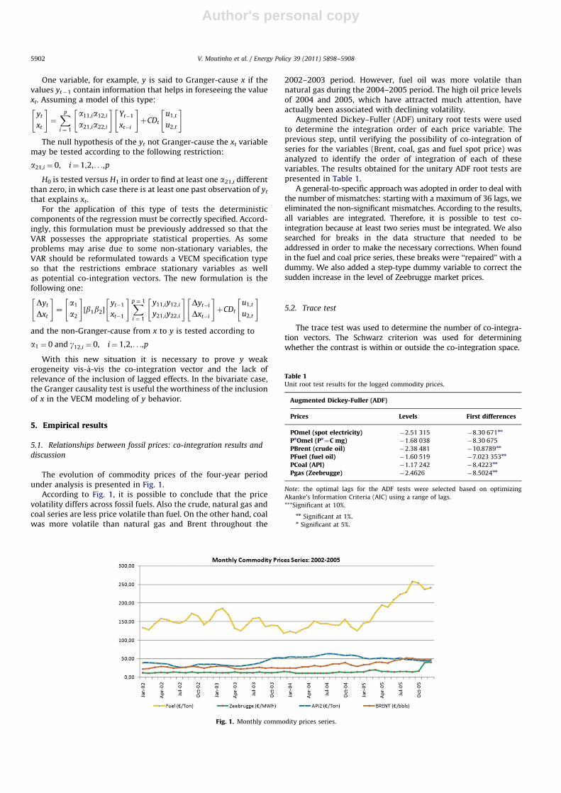
The evolution of commodity prices of the four-year periodunder analysis is presented in Fig. 1.

According to Fig. 1, it is possible to conclude that the pricevolatility differs across fossil fuels. Also the crude, natural gas andcoal series are less price volatile than fuel. On the other hand, coalwas more volatile than natural gas and Brent throughout the

2002–2003 period. However, fuel oil was more volatile thannatural gas during the 2004–2005 period. The high oil price levelsof 2004 and 2005, which have attracted much attention, haveactually been associated with declining volatility.

Augmented Dickey–Fuller (ADF) unitary root tests were usedto determine the integration order of each price variable. Theprevious step, until verifying the possibility of co-integration ofseries for the variables (Brent, coal, gas and fuel spot price) wasanalyzed to identify the order of integration of each of thesevariables. The results obtained for the unitary ADF root tests arepresented in Table 1.

A general-to-specific approach was adopted in order to deal withthe number of mismatches: starting with a maximum of 36 lags, weeliminated the non-significant mismatches. According to the results,all variables are integrated. Therefore, it is possible to test co-integration because at least two series must be integrated. We alsosearched for breaks in the data structure that needed to beaddressed in order to make the necessary corrections. When foundin the fuel and coal price series, these breaks were ‘‘repaired’’ with adummy. We also added a step-type dummy variable to correct thesudden increase in the level of Zeebrugge market prices.

5.2. Trace test

The trace test was used to determine the number of co-integra-tion vectors. The Schwarz criterion was used for determiningwhether the contrast is within or outside the co-integration space.

Fig. 1. Monthly commodity prices series.

Table 1Unit root test results for the logged commodity prices.

Augmented Dickey-Fuller (ADF)

Prices Levels First differences

POmel (spot electricity) �2.51 315 �8.30 671nn

PnOmel (Pn¼C mg) �1.68 038 �8.30 675

PBrent (crude oil) �2.38 481 �10.8789nn

PFuel (fuel oil) �1.60 519 �7.023 353nn

PCoal (API) �1.17 242 �8.4223nn

Pgas (Zeebrugge) �2.4626 �8.5024nn

Note: the optimal lags for the ADF tests were selected based on optimizing

Akanke’s Information Criteria (AIC) using a range of lags.

***Significant at 10%.

nn Significant at 1%.n Significant at 5%.

V. Moutinho et al. / Energy Policy 39 (2011) 5898–59085902

Author's personal copy

This test is performed sequentially starting with the assump-tion that the trace P is zero, i.e., r¼0, against the alternativehypothesis rZ1. If H0 is rejected then it is tested rr1 againstr41. Whenever the null hypothesis is rejected, the test continuesuntil H0:rr1(n�1). If no test rejects the null hypothesis, the teststops and it is concluded that there are as many co-integratingvectors as rejections of the null hypotheses, occurring as a resultof the test.

According to the achieved outputs, the statistics tests and thecritical values for different ranks (when the constant is within theco-integration space) are shown in Table 2.

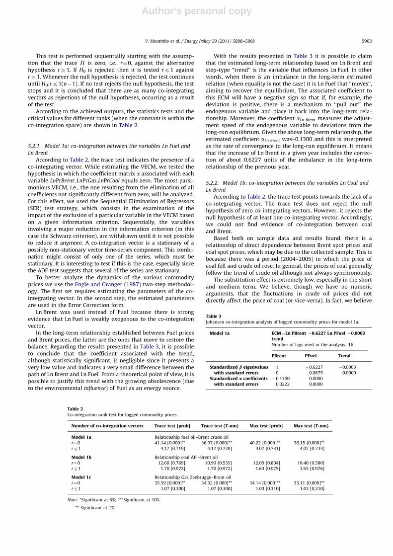
5.2.1. Model 1a: co-integration between the variables Ln Fuel and

Ln Brent

According to Table 2, the trace test indicates the presence of aco-integrating vector. While estimating the VECM, we tested thehypothesis in which the coefficient matrix a associated with eachvariable LnPrBrent; LnPrGas,LnPrCoal equals zero. The most parsi-monious VECM, i.e., the one resulting from the elimination of allcoefficients not significantly different from zero, will be analyzed.For this effect, we used the Sequential Elimination of Regressors(SER) test strategy, which consists in the examination of theimpact of the exclusion of a particular variable in the VECM basedon a given information criterion. Sequentially, the variablesinvolving a major reduction in the information criterion (in thiscase the Schwarz criterion), are withdrawn until it is not possibleto reduce it anymore. A co-integration vector is a stationary of apossibly non-stationary vector time-series component. This combi-nation might consist of only one of the series, which must bestationary. It is interesting to test if this is the case, especially sincethe ADF test suggests that several of the series are stationary.

To better analyze the dynamics of the various commodityprices we use the Engle and Granger (1987) two-step methodol-ogy. The first set requires estimating the parameters of the co-integrating vector. In the second step, the estimated parametersare used in the Error Correction form.

Ln Brent was used instead of Fuel because there is strongevidence that Ln Fuel is weakly exogenous to the co-integrationvector.

In the long-term relationship established between Fuel pricesand Brent prices, the latter are the ones that move to restore thebalance. Regarding the results presented in Table 3, it is possibleto conclude that the coefficient associated with the trend,although statistically significant, is negligible since it presents avery low value and indicates a very small difference between thepath of Ln Brent and Ln Fuel. From a theoretical point of view, it ispossible to justify this trend with the growing obsolescence (dueto the environmental influence) of Fuel as an energy source.

With the results presented in Table 3 it is possible to claimthat the estimated long-term relationship based on Ln Brent andstep-type ‘‘trend’’ is the variable that influences Ln Fuel. In otherwords, when there is an imbalance in the long-term estimatedrelation (when equality is not the case) it is Ln Fuel that ‘‘moves’’,aiming to recover the equilibrium. The associated coefficient tothis ECM will have a negative sign so that if, for example, thedeviation is positive, there is a mechanism to ‘‘pull out’’ theendogenous variable and place it back into the long-term rela-tionship. Moreover, the coefficient aLn Brent measures the adjust-ment speed of the endogenous variable to deviations from thelong-run equilibrium. Given the above long-term relationship, theestimated coefficient aLn Brent was–0.1300 and this is interpretedas the rate of convergence to the long-run equilibrium. It meansthat the increase of Ln Brent in a given year includes the correc-tion of about 0.6227 units of the imbalance in the long-termrelationship of the previous year.

5.2.2. Model 1b: co-integration between the variables Ln Coal and

Ln Brent

According to Table 2, the trace test points towards the lack of aco-integrating vector. The trace test does not reject the nullhypothesis of zero co-integrating vectors. However, it rejects thenull hypothesis of at least one co-integrating vector. Accordingly,we could not find evidence of co-integration between coaland Brent.

Based both on sample data and results found, there is arelationship of direct dependence between Brent spot prices andcoal spot prices, which may be due to the collected sample. This isbecause there was a period (2004–2005) in which the price ofcoal fell and crude oil rose. In general, the prices of coal generallyfollow the trend of crude oil although not always synchronously.

The substitution effect is extremely low, especially in the shortand medium term. We believe, though we have no numericarguments, that the fluctuations in crude oil prices did notdirectly affect the price of coal (or vice-versa). In fact, we believe

Table 2Co-integration rank test for logged commodity prices.

Number of co-integration vectors Trace test [prob] Trace test (T-nm) Max test [prob] Max test (T-nm)

Model 1a Relationship fuel oil–Brent crude oil

r¼0 41.14 [0.000]nn 36.97 [0.000]nn 40.22 [0.000]nn 36.15 [0.000]nn

rr1 4.17 [0.719] 4.17 [0.720] 4.07 [0.731] 4.07 [0.733]

Model 1b Relationship coal API–Brent oil

r¼0 12.60 [0.769] 10.90 [0.535] 12.09 [0.804] 10.46 [0.580]

rr1 1.70 [0.972] 1.70 [0.972] 1.63 [0.975] 1.63 [0.976]

Model 1c Relationship Gas Zeebrugge–Brent oil

r¼0 35.59 [0.000]nn 34.52 [0.000]nn 34.14 [0.000]nn 33.11 [0.000]nn

rr1 1.07 [0.300] 1.07 [0.300] 1.03 [0.310] 1.03 [0,310]

Note: *Significant at 5%; ***Significant at 10%.

nn Significant at 1%.

Table 3Johansen co-integration analysis of logged commodity prices for model 1a.

Model 1a ECM¼Ln PBrent �0.6227 Ln PFuel �0.0003trendNumber of lags used in the analysis: 16

PBrent PFuel Trend

Standardized b eigenvalueswith standard errors

1 �0.6227 �0.0003

0 0.0875 0.0000

Standardized a coefficientswith standard errors

�0.1300 0.0000

0.0222 0.0000

V. Moutinho et al. / Energy Policy 39 (2011) 5898–5908 5903

Author's personal copy

that the harmonious oscillation between both energy products isbased on the worldwide pressure of demand for energy.

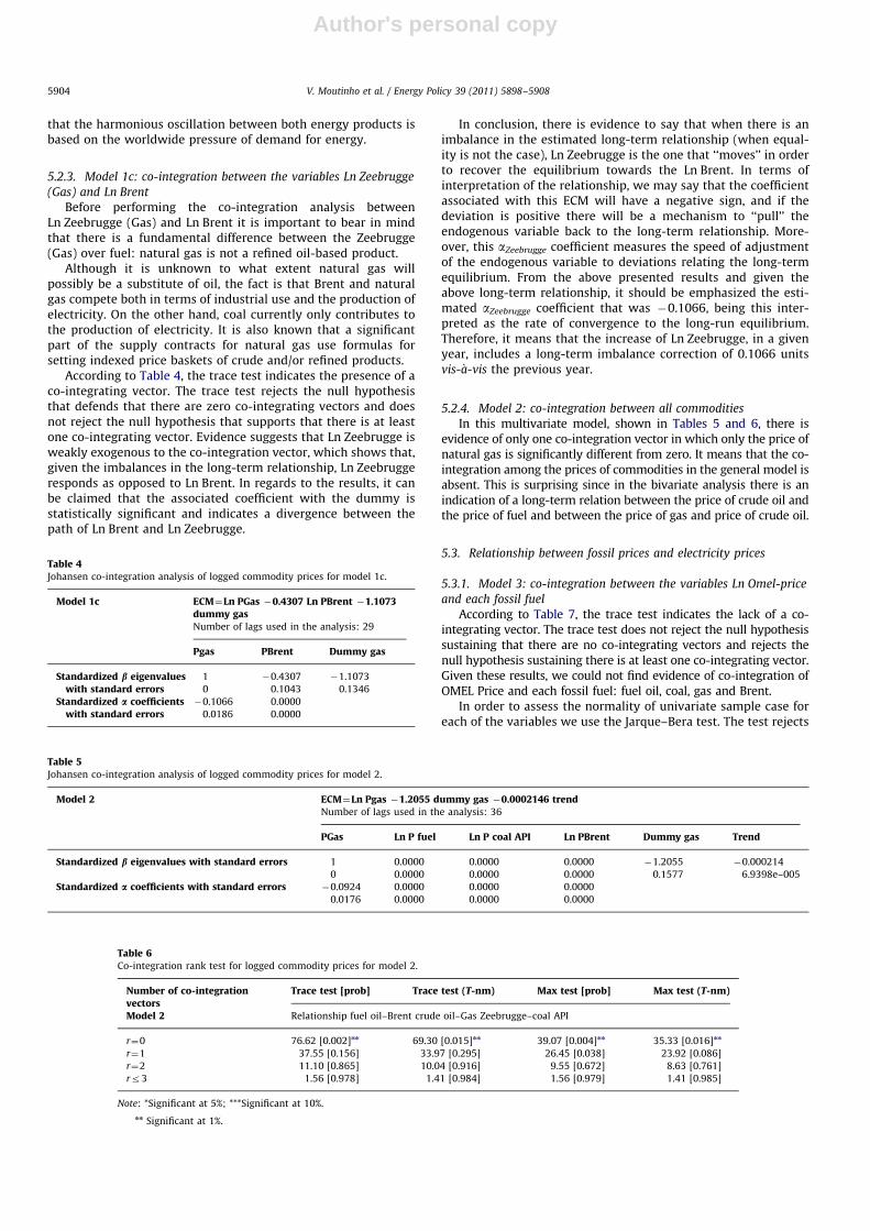
5.2.3. Model 1c: co-integration between the variables Ln Zeebrugge

(Gas) and Ln Brent

Before performing the co-integration analysis betweenLn Zeebrugge (Gas) and Ln Brent it is important to bear in mindthat there is a fundamental difference between the Zeebrugge(Gas) over fuel: natural gas is not a refined oil-based product.

Although it is unknown to what extent natural gas willpossibly be a substitute of oil, the fact is that Brent and naturalgas compete both in terms of industrial use and the production ofelectricity. On the other hand, coal currently only contributes tothe production of electricity. It is also known that a significantpart of the supply contracts for natural gas use formulas forsetting indexed price baskets of crude and/or refined products.

According to Table 4, the trace test indicates the presence of aco-integrating vector. The trace test rejects the null hypothesisthat defends that there are zero co-integrating vectors and doesnot reject the null hypothesis that supports that there is at leastone co-integrating vector. Evidence suggests that Ln Zeebrugge isweakly exogenous to the co-integration vector, which shows that,given the imbalances in the long-term relationship, Ln Zeebruggeresponds as opposed to Ln Brent. In regards to the results, it canbe claimed that the associated coefficient with the dummy isstatistically significant and indicates a divergence between thepath of Ln Brent and Ln Zeebrugge.

In conclusion, there is evidence to say that when there is animbalance in the estimated long-term relationship (when equal-ity is not the case), Ln Zeebrugge is the one that ‘‘moves’’ in orderto recover the equilibrium towards the Ln Brent. In terms ofinterpretation of the relationship, we may say that the coefficientassociated with this ECM will have a negative sign, and if thedeviation is positive there will be a mechanism to ‘‘pull’’ theendogenous variable back to the long-term relationship. More-over, this aZeebrugge coefficient measures the speed of adjustmentof the endogenous variable to deviations relating the long-termequilibrium. From the above presented results and given theabove long-term relationship, it should be emphasized the esti-mated aZeebrugge coefficient that was �0.1066, being this inter-preted as the rate of convergence to the long-run equilibrium.Therefore, it means that the increase of Ln Zeebrugge, in a givenyear, includes a long-term imbalance correction of 0.1066 unitsvis-�a-vis the previous year.

5.2.4. Model 2: co-integration between all commodities

In this multivariate model, shown in Tables 5 and 6, there isevidence of only one co-integration vector in which only the price ofnatural gas is significantly different from zero. It means that the co-integration among the prices of commodities in the general model isabsent. This is surprising since in the bivariate analysis there is anindication of a long-term relation between the price of crude oil andthe price of fuel and between the price of gas and price of crude oil.

5.3. Relationship between fossil prices and electricity prices

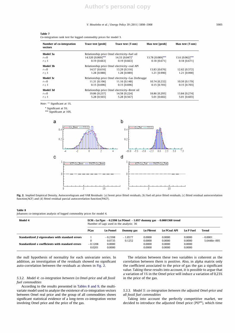
5.3.1. Model 3: co-integration between the variables Ln Omel-price

and each fossil fuel

According to Table 7, the trace test indicates the lack of a co-integrating vector. The trace test does not reject the null hypothesissustaining that there are no co-integrating vectors and rejects thenull hypothesis sustaining there is at least one co-integrating vector.Given these results, we could not find evidence of co-integration ofOMEL Price and each fossil fuel: fuel oil, coal, gas and Brent.

In order to assess the normality of univariate sample case foreach of the variables we use the Jarque–Bera test. The test rejects

Table 4Johansen co-integration analysis of logged commodity prices for model 1c.

Model 1c ECM¼Ln PGas �0.4307 Ln PBrent �1.1073dummy gasNumber of lags used in the analysis: 29

Pgas PBrent Dummy gas

Standardized b eigenvalueswith standard errors

1 �0.4307 �1.1073

0 0.1043 0.1346

Standardized a coefficientswith standard errors

�0.1066 0.0000

0.0186 0.0000

Table 5Johansen co-integration analysis of logged commodity prices for model 2.

Model 2 ECM¼Ln Pgas �1.2055 dummy gas �0.0002146 trendNumber of lags used in the analysis: 36

PGas Ln P fuel Ln P coal API Ln PBrent Dummy gas Trend

Standardized b eigenvalues with standard errors 1 0.0000 0.0000 0.0000 �1.2055 �0.000214

0 0.0000 0.0000 0.0000 0.1577 6.9398e–005

Standardized a coefficients with standard errors �0.0924 0.0000 0.0000 0.0000

0.0176 0.0000 0.0000 0.0000

Table 6Co-integration rank test for logged commodity prices for model 2.

Number of co-integrationvectors

Trace test [prob] Trace test (T-nm) Max test [prob] Max test (T-nm)

Model 2 Relationship fuel oil–Brent crude oil–Gas Zeebrugge–coal API

r¼0 76.62 [0.002]nn 69.30 [0.015]nn 39.07 [0.004]nn 35.33 [0.016]nn

r¼1 37.55 [0.156] 33.97 [0.295] 26.45 [0.038] 23.92 [0.086]

r¼2 11.10 [0.865] 10.04 [0.916] 9.55 [0.672] 8.63 [0.761]

rr3 1.56 [0.978] 1.41 [0.984] 1.56 [0.979] 1.41 [0.985]

Note: *Significant at 5%; ***Significant at 10%.

nn Significant at 1%.

V. Moutinho et al. / Energy Policy 39 (2011) 5898–59085904

Author's personal copy

the null hypothesis of normality for each univariate series. Inaddition, an investigation of the residuals showed no significantauto-correlation between the residuals as shown in Fig. 2.

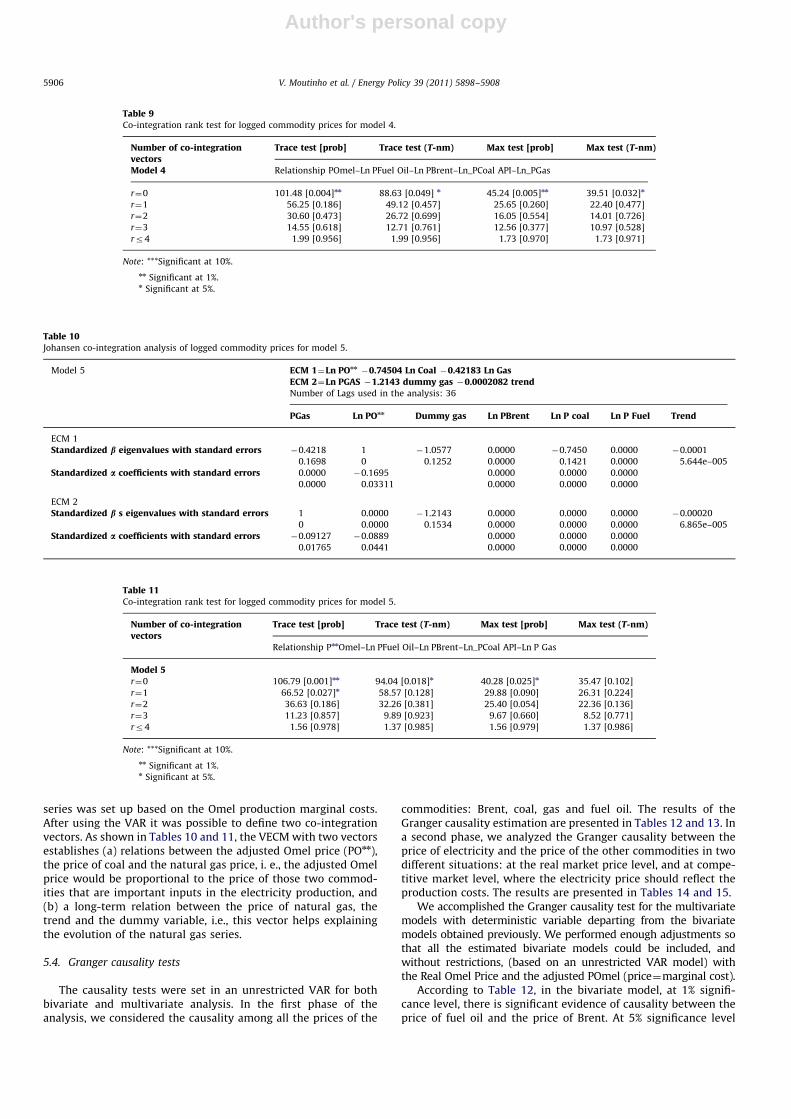
5.3.2. Model 4: co-integration between Ln Omel-price and all fossil

fuel commodities

According to the results presented in Tables 8 and 9, the multi-variate model used to analyze the existence of co-integration vectorsbetween Omel real price and the group of all commodities showssignificant statistical evidence of a long-term co-integration vectorinvolving Omel price and the price of the gas.

The relation between these two variables is coherent as thecorrelation between them is positive. Also, in alpha matrix onlythe coefficient associated to the price of gas the gas a significantvalue. Taking these results into account, it is possible to argue thata variation of 1% in the Omel price will induce a variation of 0,23%in the price of the gas.

5.3.3. Model 5: co-integration between the adjusted Omel-price and

all fossil fuel commodities

Taking into account the perfectly competitive market, wedecided to introduce the adjusted Omel price (POnn), which time

Table 7Co-integration rank test for logged commodity prices for model 3.

Number of co-integrationvectors

Trace test [prob] Trace test (T-nm) Max test [prob] Max test (T-nm)

Model 3a Relationship price Omel electricity–fuel oil

r¼0 14.520 [0.069]nnn 14.33 [0.047]n 13.78 [0.089]nnn 13.6 [0.062]nnn

rr1 0.19 [0.663] 0.19 [0.663] 0.18 [0.671] 0.18 [0.671]

Model 3b Relationship price Omel electricity–coal API

r¼0 14.57 [0.616] 13.29 [0.316] 13.83 [0.676] 12.62 [0.372]

rr1 1.28 [0.988] 1.28 [0.989] 1.21 [0.990] 1.21 [0.990]

Model 3c Relationship price Omel electricity–Gas Zeebrugge

r¼0 11.31 [0.196] 11.16 [0.148] 10.74 [0.232] 10.59 [0.179]

rr1 0.15 [0.696] 0.15 [0.696] 0.15 [0.703] 0.15 [0.703]

Model 3d Relationship price Omel electricity–Brent oil

r¼0 19.86 [0.237] 14.58 [0.224] 18.86 [0.295] 13.84 [0.274]

rr1 5.28 [0.565] 5.28 [0.567] 5.01 [0.602] 5.01 [0.603]

Note: ** Significant at 1%.

n Significant at 5%.nnn Significant at 10%.

Fig. 2. Implied Empirical Density, Autocorrelogram and VAR Residuals: (a) brent price fitted residuals, (b) fuel oil price fitted residuals, (c) fitted residual autocorrelation

function(ACF) and (d) fitted residual parcial autocorrelation function(PACF).

Table 8Johansen co-integration analysis of logged commodity prices for model 4.

Model 4 ECM¼Ln Pgas �0.2398 Ln POmel �1.057 dummy gas �0.0001368 trendNumber of Lags used in the analysis: 36

PGas Ln Pomel Dummy gas Ln PBrent Ln PCoal API Ln P Fuel Trend

Standardized b eigenvalues with standard errors 1 �0.2398 �1.0577 0.0000 0.0000 0.0000 �0.0001

0 0.0735 0.1252 0.0000 0.0000 0.0000 5.6448e–005

Standardized a coefficients with standard errors �0.1208 0.0000 0.0000 0.0000 0.0000

0.0201 0.0000 0.0000 0.0000 0.0000

V. Moutinho et al. / Energy Policy 39 (2011) 5898–5908 5905

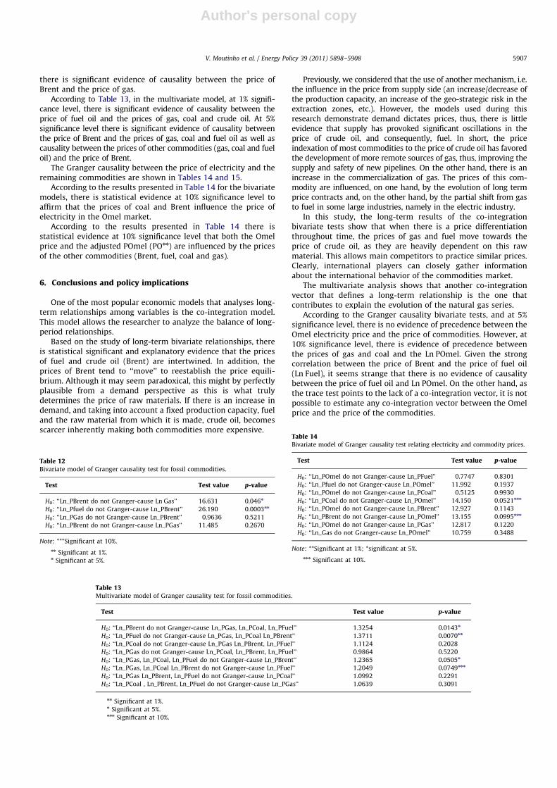
Author's personal copy

series was set up based on the Omel production marginal costs.After using the VAR it was possible to define two co-integrationvectors. As shown in Tables 10 and 11, the VECM with two vectorsestablishes (a) relations between the adjusted Omel price (POnn),the price of coal and the natural gas price, i. e., the adjusted Omelprice would be proportional to the price of those two commod-ities that are important inputs in the electricity production, and(b) a long-term relation between the price of natural gas, thetrend and the dummy variable, i.e., this vector helps explainingthe evolution of the natural gas series.

5.4. Granger causality tests

The causality tests were set in an unrestricted VAR for bothbivariate and multivariate analysis. In the first phase of theanalysis, we considered the causality among all the prices of the

commodities: Brent, coal, gas and fuel oil. The results of theGranger causality estimation are presented in Tables 12 and 13. Ina second phase, we analyzed the Granger causality between theprice of electricity and the price of the other commodities in twodifferent situations: at the real market price level, and at compe-titive market level, where the electricity price should reflect theproduction costs. The results are presented in Tables 14 and 15.

We accomplished the Granger causality test for the multivariatemodels with deterministic variable departing from the bivariatemodels obtained previously. We performed enough adjustments sothat all the estimated bivariate models could be included, andwithout restrictions, (based on an unrestricted VAR model) withthe Real Omel Price and the adjusted POmel (price¼marginal cost).

According to Table 12, in the bivariate model, at 1% signifi-cance level, there is significant evidence of causality between theprice of fuel oil and the price of Brent. At 5% significance level

Table 9Co-integration rank test for logged commodity prices for model 4.

Number of co-integrationvectors

Trace test [prob] Trace test (T-nm) Max test [prob] Max test (T-nm)

Model 4 Relationship POmel–Ln PFuel Oil–Ln PBrent–Ln_PCoal API–Ln_PGas

r¼0 101.48 [0.004]nn 88.63 [0.049] n 45.24 [0.005]nn 39.51 [0.032]n

r¼1 56.25 [0.186] 49.12 [0.457] 25.65 [0.260] 22.40 [0.477]

r¼2 30.60 [0.473] 26.72 [0.699] 16.05 [0.554] 14.01 [0.726]

r¼3 14.55 [0.618] 12.71 [0.761] 12.56 [0.377] 10.97 [0.528]

rr4 1.99 [0.956] 1.99 [0.956] 1.73 [0.970] 1.73 [0.971]

Note: ***Significant at 10%.

nn Significant at 1%.n Significant at 5%.

Table 10Johansen co-integration analysis of logged commodity prices for model 5.

Model 5 ECM 1¼Ln POnn�0.74504 Ln Coal �0.42183 Ln Gas

ECM 2¼Ln PGAS �1.2143 dummy gas �0.0002082 trendNumber of Lags used in the analysis: 36

PGas Ln POnn Dummy gas Ln PBrent Ln P coal Ln P Fuel Trend

ECM 1

Standardized b eigenvalues with standard errors �0.4218 1 �1.0577 0.0000 �0.7450 0.0000 �0.0001

0.1698 0 0.1252 0.0000 0.1421 0.0000 5.644e–005

Standardized a coefficients with standard errors 0.0000 �0.1695 0.0000 0.0000 0.0000

0.0000 0.03311 0.0000 0.0000 0.0000

ECM 2

Standardized b s eigenvalues with standard errors 1 0.0000 �1.2143 0.0000 0.0000 0.0000 �0.00020

0 0.0000 0.1534 0.0000 0.0000 0.0000 6.865e–005

Standardized a coefficients with standard errors �0.09127 �0.0889 0.0000 0.0000 0.0000

0.01765 0.0441 0.0000 0.0000 0.0000

Table 11Co-integration rank test for logged commodity prices for model 5.

Number of co-integrationvectors

Trace test [prob] Trace test (T-nm) Max test [prob] Max test (T-nm)

Relationship PnnOmel–Ln PFuel Oil–Ln PBrent–Ln_PCoal API–Ln P Gas

Model 5r¼0 106.79 [0.001]nn 94.04 [0.018]n 40.28 [0.025]n 35.47 [0.102]

r¼1 66.52 [0.027]n 58.57 [0.128] 29.88 [0.090] 26.31 [0.224]

r¼2 36.63 [0.186] 32.26 [0.381] 25.40 [0.054] 22.36 [0.136]

r¼3 11.23 [0.857] 9.89 [0.923] 9.67 [0.660] 8.52 [0.771]

rr4 1.56 [0.978] 1.37 [0.985] 1.56 [0.979] 1.37 [0.986]

Note: ***Significant at 10%.

nn Significant at 1%.n Significant at 5%.

V. Moutinho et al. / Energy Policy 39 (2011) 5898–59085906

Author's personal copy

there is significant evidence of causality between the price ofBrent and the price of gas.

According to Table 13, in the multivariate model, at 1% signifi-cance level, there is significant evidence of causality between theprice of fuel oil and the prices of gas, coal and crude oil. At 5%significance level there is significant evidence of causality betweenthe price of Brent and the prices of gas, coal and fuel oil as well ascausality between the prices of other commodities (gas, coal and fueloil) and the price of Brent.

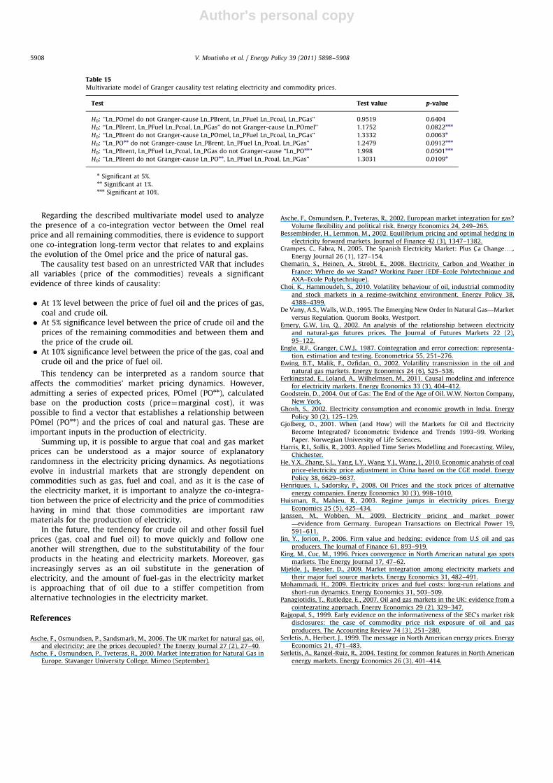
The Granger causality between the price of electricity and theremaining commodities are shown in Tables 14 and 15.

According to the results presented in Table 14 for the bivariatemodels, there is statistical evidence at 10% significance level toaffirm that the prices of coal and Brent influence the price ofelectricity in the Omel market.

According to the results presented in Table 14 there isstatistical evidence at 10% significance level that both the Omelprice and the adjusted POmel (POnn) are influenced by the pricesof the other commodities (Brent, fuel, coal and gas).

6. Conclusions and policy implications

One of the most popular economic models that analyses long-term relationships among variables is the co-integration model.This model allows the researcher to analyze the balance of long-period relationships.

Based on the study of long-term bivariate relationships, thereis statistical significant and explanatory evidence that the pricesof fuel and crude oil (Brent) are intertwined. In addition, theprices of Brent tend to ‘‘move’’ to reestablish the price equili-brium. Although it may seem paradoxical, this might by perfectlyplausible from a demand perspective as this is what trulydetermines the price of raw materials. If there is an increase indemand, and taking into account a fixed production capacity, fueland the raw material from which it is made, crude oil, becomesscarcer inherently making both commodities more expensive.

Previously, we considered that the use of another mechanism, i.e.the influence in the price from supply side (an increase/decrease ofthe production capacity, an increase of the geo-strategic risk in theextraction zones, etc.). However, the models used during thisresearch demonstrate demand dictates prices, thus, there is littleevidence that supply has provoked significant oscillations in theprice of crude oil, and consequently, fuel. In short, the priceindexation of most commodities to the price of crude oil has favoredthe development of more remote sources of gas, thus, improving thesupply and safety of new pipelines. On the other hand, there is anincrease in the commercialization of gas. The prices of this com-modity are influenced, on one hand, by the evolution of long termprice contracts and, on the other hand, by the partial shift from gasto fuel in some large industries, namely in the electric industry.

In this study, the long-term results of the co-integrationbivariate tests show that when there is a price differentiationthroughout time, the prices of gas and fuel move towards theprice of crude oil, as they are heavily dependent on this rawmaterial. This allows main competitors to practice similar prices.Clearly, international players can closely gather informationabout the international behavior of the commodities market.

The multivariate analysis shows that another co-integrationvector that defines a long-term relationship is the one thatcontributes to explain the evolution of the natural gas series.

According to the Granger causality bivariate tests, and at 5%significance level, there is no evidence of precedence between theOmel electricity price and the price of commodities. However, at10% significance level, there is evidence of precedence betweenthe prices of gas and coal and the Ln POmel. Given the strongcorrelation between the price of Brent and the price of fuel oil(Ln Fuel), it seems strange that there is no evidence of causalitybetween the price of fuel oil and Ln POmel. On the other hand, asthe trace test points to the lack of a co-integration vector, it is notpossible to estimate any co-integration vector between the Omelprice and the price of the commodities.

Table 12Bivariate model of Granger causality test for fossil commodities.

Test Test value p-value

H0: ‘‘Ln_PBrent do not Granger-cause Ln Gas’’ 16.631 0.046n

H0: ‘‘Ln_Pfuel do not Granger-cause Ln_PBrent’’ 26.190 0.0003nn

H0: ‘‘Ln_PGas do not Granger-cause Ln_PBrent’’ 0.9636 0.5211

H0: ‘‘Ln_PBrent do not Granger-cause Ln_PGas’’ 11.485 0.2670

Note: ***Significant at 10%.

nn Significant at 1%.n Significant at 5%.

Table 13Multivariate model of Granger causality test for fossil commodities.

Test Test value p-value

H0: ‘‘Ln_PBrent do not Granger-cause Ln_PGas, Ln_PCoal, Ln_PFuel’’ 1.3254 0.0143n

H0: ‘‘Ln_PFuel do not Granger-cause Ln_PGas, Ln_PCoal Ln_PBrent’’ 1.3711 0.0070nn

H0: ‘‘Ln_PCoal do not Granger-cause Ln_PGas Ln_PBrent, Ln_PFuel’’ 1.1124 0.2028

H0: ‘‘Ln_PGas do not Granger-cause Ln_PCoal, Ln_PBrent, Ln_PFuel’’ 0.9864 0.5220

H0: ‘‘Ln_PGas, Ln_PCoal, Ln_PFuel do not Granger-cause Ln_PBrent’’ 1.2365 0.0505n

H0: ‘‘Ln_PGas, Ln_PCoal Ln_PBrent do not Granger-cause Ln_PFuel’’ 1.2049 0.0749nnn

H0: ‘‘Ln_PGas Ln_PBrent, Ln_PFuel do not Granger-cause Ln_PCoal’’ 1.0992 0.2291

H0: ‘‘Ln_PCoal , Ln_PBrent, Ln_PFuel do not Granger-cause Ln_PGas’’ 1.0639 0.3091

nn Significant at 1%.n Significant at 5%.nnn Significant at 10%.

Table 14Bivariate model of Granger causality test relating electricity and commodity prices.

Test Test value p-value

H0: ‘‘Ln_POmel do not Granger-cause Ln_PFuel’’ 0.7747 0.8301

H0: ‘‘Ln_Pfuel do not Granger-cause Ln_POmel’’ 11.992 0.1937

H0: ‘‘Ln_POmel do not Granger-cause Ln_PCoal’’ 0.5125 0.9930

H0: ‘‘Ln_PCoal do not Granger-cause Ln_POmel’’ 14.150 0.0521nnn

H0: ‘‘Ln_POmel do not Granger-cause Ln_PBrent’’ 12.927 0.1143

H0: ‘‘Ln_PBrent do not Granger-cause Ln_POmel’’ 13.155 0.0995nnn

H0: ‘‘Ln_POmel do not Granger-cause Ln_PGas’’ 12.817 0.1220

H0: ‘‘Ln_Gas do not Granger-cause Ln_POmel’’ 10.759 0.3488

Note: **Significant at 1%; *significant at 5%.

nnn Significant at 10%.

V. Moutinho et al. / Energy Policy 39 (2011) 5898–5908 5907

Author's personal copy

Regarding the described multivariate model used to analyzethe presence of a co-integration vector between the Omel realprice and all remaining commodities, there is evidence to supportone co-integration long-term vector that relates to and explainsthe evolution of the Omel price and the price of natural gas.

The causality test based on an unrestricted VAR that includesall variables (price of the commodities) reveals a significantevidence of three kinds of causality:

� At 1% level between the price of fuel oil and the prices of gas,coal and crude oil.� At 5% significance level between the price of crude oil and the

prices of the remaining commodities and between them andthe price of the crude oil.� At 10% significance level between the price of the gas, coal and

crude oil and the price of fuel oil.

This tendency can be interpreted as a random source thataffects the commodities’ market pricing dynamics. However,admitting a series of expected prices, POmel (POnn), calculatedbase on the production costs (price¼marginal cost), it waspossible to find a vector that establishes a relationship betweenPOmel (POnn) and the prices of coal and natural gas. These areimportant inputs in the production of electricity.

Summing up, it is possible to argue that coal and gas marketprices can be understood as a major source of explanatoryrandomness in the electricity pricing dynamics. As negotiationsevolve in industrial markets that are strongly dependent oncommodities such as gas, fuel and coal, and as it is the case ofthe electricity market, it is important to analyze the co-integra-tion between the price of electricity and the price of commoditieshaving in mind that those commodities are important rawmaterials for the production of electricity.

In the future, the tendency for crude oil and other fossil fuelprices (gas, coal and fuel oil) to move quickly and follow oneanother will strengthen, due to the substitutability of the fourproducts in the heating and electricity markets. Moreover, gasincreasingly serves as an oil substitute in the generation ofelectricity, and the amount of fuel-gas in the electricity marketis approaching that of oil due to a stiffer competition fromalternative technologies in the electricity market.

References

Asche, F., Osmundsen, P., Sandsmark, M., 2006. The UK market for natural gas, oil,and electricity: are the prices decoupled? The Energy Journal 27 (2), 27–40.

Asche, F., Osmundsen, P., Tveteras, R., 2000. Market Integration for Natural Gas inEurope. Stavanger University College, Mimeo (September).

Asche, F., Osmundsen, P., Tveteras, R., 2002. European market integration for gas?Volume flexibility and political risk. Energy Economics 24, 249–265.

Bessembinder, H., Lemmon, M., 2002. Equilibrium pricing and optimal hedging inelectricity forward markets. Journal of Finance 42 (3), 1347–1382.

Crampes, C., Fabra, N., 2005. The Spanish Electricity Market: Plus C- a Changey,.Energy Journal 26 (1), 127–154.

Chemarin, S., Heinen, A., Strobl, E., 2008. Electricity, Carbon and Weather inFrance: Where do we Stand? Working Paper (EDF–Ecole Polytechnique andAXA–Ecole Polytechnique).

Choi, K., Hammoudeh, S., 2010. Volatility behaviour of oil, industrial commodityand stock markets in a regime-switching environment. Energy Policy 38,4388–4399.

De Vany, A.S., Walls, W.D., 1995. The Emerging New Order In Natural Gas—Marketversus Regulation. Quorum Books, Westport.

Emery, G.W, Liu, Q., 2002. An analysis of the relationship between electricityand natural-gas futures prices. The Journal of Futures Markets 22 (2),95–122.

Engle, R.F., Granger, C.W.J., 1987. Cointegration and error correction: representa-tion, estimation and testing. Econometrica 55, 251–276.

Ewing, B.T., Malik, F., Ozfidan, O., 2002. Volatility transmission in the oil andnatural gas markets. Energy Economics 24 (6), 525–538.

Ferkingstad, E., Loland, A., Wilhelmsen, M., 2011. Causal modeling and inferencefor electricity markets. Energy Economics 33 (3), 404–412.

Goodstein, D., 2004. Out of Gas: The End of the Age of Oil. W.W. Norton Company,New York.

Ghosh, S., 2002. Electricity consumption and economic growth in India. EnergyPolicy 30 (2), 125–129.

Gjolberg, O., 2001. When (and How) will the Markets for Oil and ElectricityBecome Integrated? Econometric Evidence and Trends 1993–99. WorkingPaper. Norwegian University of Life Sciences.

Harris, R.I., Sollis, R., 2003. Applied Time Series Modelling and Forecasting. Wiley,Chichester.

He, Y.X., Zhang, S.L., Yang, L.Y., Wang, Y.J., Wang, J., 2010. Economic analysis of coalprice-electricity price adjustment in China based on the CGE model. EnergyPolicy 38, 6629–6637.

Henriques, I., Sadorsky, P., 2008. Oil Prices and the stock prices of alternativeenergy companies. Energy Economics 30 (3), 998–1010.

Huisman, R., Mahieu, R., 2003. Regime jumps in electricity prices. EnergyEconomics 25 (5), 425–434.

Janssen, M., Wobben, M., 2009. Electricity pricing and market power—evidence from Germany. European Transactions on Electrical Power 19,591–611.

Jin, Y., Jorion, P., 2006. Firm value and hedging: evidence from U.S oil and gasproducers. The Journal of Finance 61, 893–919.

King, M., Cuc, M., 1996. Prices convergence in North American natural gas spotsmarkets. The Energy Journal 17, 47–62.

Mjelde, J., Bessler, D., 2009. Market integration among electricity markets andtheir major fuel source markets. Energy Economics 31, 482–491.

Mohammadi, H., 2009. Electricity prices and fuel costs: long-run relations andshort-run dynamics. Energy Economics 31, 503–509.

Panagiotidis, T., Rutledge, E., 2007. Oil and gas markets in the UK: evidence from acointegrating approach. Energy Economics 29 (2), 329–347.

Rajgopal, S., 1999. Early evidence on the informativeness of the SEC’s market riskdisclosures: the case of commodity price risk exposure of oil and gasproducers. The Accounting Review 74 (3), 251–280.

Serletis, A., Herbert, J., 1999. The message in North American energy prices. EnergyEconomics 21, 471–483.

Serletis, A., Rangel-Ruiz, R., 2004. Testing for common features in North Americanenergy markets. Energy Economics 26 (3), 401–414.

Table 15Multivariate model of Granger causality test relating electricity and commodity prices.

Test Test value p-value

H0: ‘‘Ln_POmel do not Granger-cause Ln_PBrent, Ln_PFuel Ln_Pcoal, Ln_PGas’’ 0.9519 0.6404

H0: ‘‘Ln_PBrent, Ln_PFuel Ln_Pcoal, Ln_PGas’’ do not Granger-cause Ln_POmel’’ 1.1752 0.0822nnn

H0: ‘‘Ln_PBrent do not Granger-cause Ln_POmel, Ln_PFuel Ln_Pcoal, Ln_PGas’’ 1.3332 0.0063n

H0: ‘‘Ln_POnn do not Granger-cause Ln_PBrent, Ln_PFuel Ln_Pcoal, Ln_PGas’’ 1.2479 0.0912nnn

H0: ‘‘Ln_PBrent, Ln_PFuel Ln_Pcoal, Ln_PGas do not Granger-cause ’’Ln_POnn’’ 1.998 0.0501nnn

H0: ‘‘Ln_PBrent do not Granger-cause Ln_POnn, Ln_PFuel Ln_Pcoal, Ln_PGas’’ 1.3031 0.0109n

n Significant at 5%.nn Significant at 1%.nnn Significant at 10%.

V. Moutinho et al. / Energy Policy 39 (2011) 5898–59085908