Measuring the Effect of Oil Prices on Wheat Futures Prices

1

Measuring the Effect of Oil Prices on Wheat Futures Prices*

Phillip A. Cartwright 1 Professor of Economics ESG Management School 25, rue Saint Ambroise 75011 Paris FRANCE

Natalija Riabko Market Analyst Market Studies Department FranceAgriMer 12 rue Henri Roi‐Tanguy 93555 Montreuil‐sous‐Bois cedex FRANCE

Abstract

This research is part of an ongoing program focused on understanding the relationships between

energy prices and prices of food commodities. Acknowledging the many empirical tests of efficient

markets, this study lends insight into the empirical validity of reverse regressions hypothesizing that

spot prices today help to predict forward rates in the future. The study is interesting for reasons of

economics and political science and well as for the statistical implications. This paper analyzes

empirically the possible relationship between wheat futures prices and spot oil prices considering the

importance of the effects of temporal aggregation and alternative model specification for the

understanding of the empirical relationships between the two markets (e.g., wheat and oil).

Evidence relevant to this analysis indicates that model specification and time series aggregation over daily, weekly and monthly aggregations will most certainly influence standard errors on parameter estimates as standard errors are likely to increase with aggregation. Therefore, t‐ratios are likely to change as well. Further, while goodness‐of‐fit measures might increase with aggregation, forecast accuracy with macro‐level aggregations might deteriorate owing to information loss. The results indicate the presence of contemporaneous causality between the variables of interest,

however, the presence of strict causality is mixed and the results do vary with units of time

aggregation. From an economics perspective, these results suggest that wheat and oil prices are

interrelated, but the extent of these relationships depends on model specification and data

aggregation. Hence, policies with implications for energy of wheat commodity prices such as oil‐for‐

food programs should take account of these relationships.

Key Words: wheat prices, crude oil prices, temporal aggregation, causal structure, forecasting

JEL Classifications: Q1, Q4, G1, D4, C1

1 Corresponding author: Professor Phillip A. Cartwright, ESG Management School, 25 rue Saint Ambroise, 75011, Paris, France. Email: [email protected]. Natalija Riabko, DBA, is Market Analyst, France AgriMer, Paris, France. Email: [email protected]. * The authors wish to thank James L. Smith, Southern Methodist University; C.F. Lee, Rutgers University; Octavio Escobar, ESG Management School; Ted Bos, University of Alabama‐Birmingham; and Josse Roussel, Université Paris Dauphine for helpful comments and criticisms.

2

1. Introduction

The primary purpose of this paper is too lend insight into the empirical validity of reverse regressions

hypothesizing that spot prices today help to predict forward rates in the future and the importance

of temporal aggregation in estimating such relationships. The study is interesting for reasons of

economics and political science as well as for econometrics and statistics. It is generally understood

that fluctuations in oil prices can endanger economic and political stability. Following Posner (2013),

these effects can be exacerbated to the extent that they are related to other commodities prices,

particularly those of food commodities. Hypothesizing transmission of effects from energy markets

to food commodity prices seems perfectly reasonable given the importance of energy as an input to

the growing, harvesting and transportation costs. Such cross‐market fluctuations are likely to be

particularly destabilizing for net importers of agricultural commodities including Middle Eastern

countries which import large quantities of wheat and corn. It is well known that the Middle East is of

critical importance for global oil production. It also imports a third of globally traded cereals. Middle

Eastern states consider food imports a strategic liability (Woertz, 2013).

As this research is focused on analyzing empirically the possible effects of oil prices on wheat futures

contract prices at a future point in time and to consider the effect of temporal aggregation on any

such relationship, the paper does not seek to directly address the issues concerning efficiency of

markets nor does it take on the task of determining price response to “fundamentals” such as

weather as in the work by Pindyck (2001) or Roll (1984). Further, while commodity prices such as

wheat and oil exhibited considerable volatility over the period of study (for example, the price of oil

rising from 70 USD in 2006 to over 140 USD in 2008, declining to just under 40 USD in 2009 and

rising to near 110 USD in 2011), this work does not address the possible rolls of basic supply and

demand shifts versus the roll of speculation (Knittel and Pindyck, 2013).

Earlier work has focused on the relationship between the energy sector and agricultural commodities

has been published by Baffles (2007), Muhammad and Kebede (2009) and Saghaian (2010). Baffels

3

(2007) reports that among non‐energy commodities, oil prices have the highest pass‐through to food

commodities and fertilizers. Muhammed and Kebede (2009) find that the emerging ethanol market

has integrated oil and corn prices. Saghaian (2010) using time‐series and directed graph theory

approaches, finds a correlation between oil and commodity prices, but the evidence of a (Granger)

causal link is mixed. In a different, but related context, Roberts and Schlenker (2013) estimate

elasticities for caloric energy from the most prominent food commodities and consider price and

quantity implication arising from the expansion of ethanol demand.

Temporal aggregation has been a frequent topic of past and recent research in economics and

finance. Problems of temporal aggregation arise frequently in economics and econometric analysis

as a consequence of using macro or aggregated data to estimate underlying micro, or disaggregate

relationships. Results from research indicate that effects of temporal aggregation can adversely

impact statistical estimation, inference and dynamic lag structures. Evidence relevant to this analysis

(Zellner and Montmarquette, 1971; Engle, R.F. and Liu, T.C., 1972; Rowe, 1976; Cartwright and Lee,

1987; Marcellino, 1999; Silvestrini and Veredas, 2005) indicates that time series aggregation will

most certainly influence standard errors on parameter estimates as standard errors are likely to

increase with aggregation. Therefore, t‐ratios are likely to change as well. While goodness‐of‐fit

measures might increase with aggregation, forecast accuracy with macro‐level aggregations might

deteriorate owing to information loss due to the averaging of observations associated with an

underlying micro‐level structure. Generally, the results show adverse effects of temporal

aggregation on statistical estimation, inference and on dynamic lag structures.

Following Silvestrini and Veredas (2005), aggregation of time series raises many issues relevant for

the practitioner. For example, if a time series can be characterized by a particular specification at one

level of aggregation, what is the correct specification at an alternative aggregation? If data are

available at both micro and macro levels of aggregation, which series should be modeled? If

information loss owing to aggregation is of concern, how best measure the information loss?

4

Following this Introduction, Section 2 provides a description of the data. In order to develop

understanding of the consequences of aggregation when modeling commodities futures contract

price data, models are estimated and evaluated at increasingly higher levels of temporal aggregation;

daily, weekly and monthly. Section 3 reports results from feasible generalized least squares (FGLS)

modeling. Models are estimated excluding and including the spot oil price. In addition, the model

including the oil price is estimated using a random coefficient framework (Swamy, 1970). Following

the early work of Cartwright and Lee (1987), analysis is made based upon aggregation and estimated

basic errors of the coefficients.

Section 4 addresses issues of time series dynamics and causality. In order to gain further

understanding of model estimation and performance, a time series approach is applied to the data

for the U.S. and France. The results for GARCH applications at the daily, weekly and monthly

aggregation levels are reported including diagnostics and forecast measures. The summary and

conclusions from the empirical work appear in the final section.

2. Data

Data are collected on futures wheat contract price and spot prices for the United States and France.

These markets are considered to be the largest for which reliable market data are available on a daily

weekly and monthly basis. .

Data are collected on a daily basis beginning on 1 January 2006 through 31 December 2011. This

period was chosen so as to begin the analysis prior to the onset of the financial crisis beginning in

2008 and ending with the final period of availability. The empirical analysis is based on the daily,

weekly and monthly FOB prices for U.S. Soft Red Winter (Gulf ports), and French Soft Wheat (Rouen)

as well as on the corresponding products futures prices. All the price series are quoted in nominal

USD per ton. The US daily spot prices and U.S. daily futures rates were taken from the International

Grain Council (IGC) data base which corresponds to Eurostat data. The French daily spot prices and

5

French daily futures prices were taken from the International Grain Council (IGC) data base which

also corresponds to Eurostat data.

The ICE Brent Crude daily spot rates and daily futures rates were taken from the International Grain

Council (IGC) data base which corresponds to International Exchange (ICE) data. The ICE Brent Crude

Futures contract is a deliverable contract based on EFP delivery with an option to cash settlement.

Data have been aggregated from daily data (n=1538) to weekly (n=308) and monthly data series

(n=68) in order to guarantee correspondence between the series over time.

3. Basic and Random Coefficient Models

3.1 Basic and Extended Models

Since the 1970s, empirical research on financial markets behavior and performance has emphasized

the efficient market hypothesis, which states that given a particular financial contract with developed

forward and spot markets, the forward price reflects all information possessed by persons active in

that market. Therefore, in an open market, the forward price should be an unbiased predictor of the

future spot price (Dornbusch, 1976). Empirical tests of this relationship take the form of a regression

1) )()()( kttfkts k

where

s (t) = the spot price on contracts of wheat at period t

f (t) = the average of the 30‐day forward contract price recorded at period t‐1

ε (t) = error disturbance assumed distributed normal and independently with zero mean

variance σ2

k number of periods into the future from the time period t.

The efficient market hypothesis implies that the estimate of the constant term is not significantly

different from zero and the estimate of β is not significant different from 1.0.

6

Note that f k(t) is 30‐day forward price. Weekly and monthly data series were constructed from daily

data averaging not only time intervals taking into account multiple contracts week‐ends and trading

holidays.

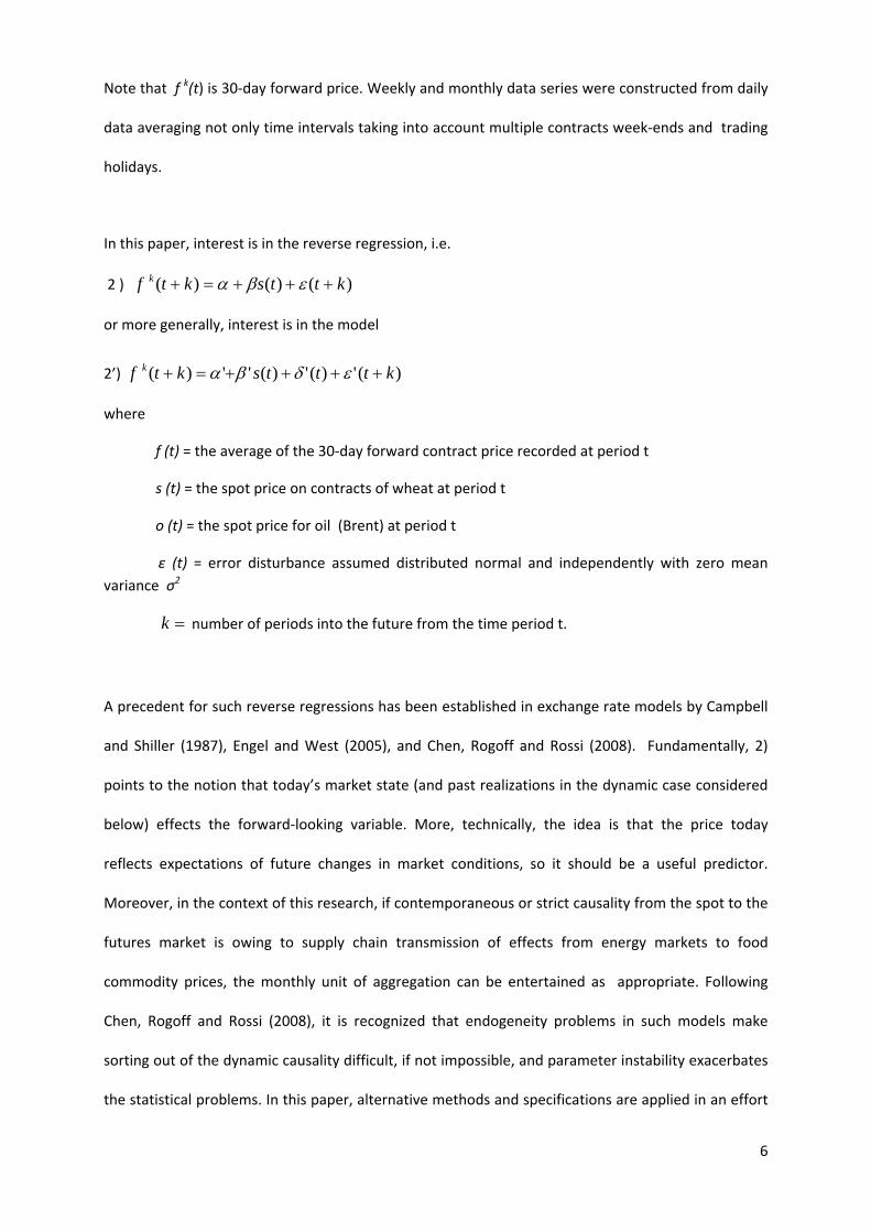
In this paper, interest is in the reverse regression, i.e.

2 ) )()()( kttsktf k

or more generally, interest is in the model

2’) )(')(')('')( ktttsktf k

where

f (t) = the average of the 30‐day forward contract price recorded at period t

s (t) = the spot price on contracts of wheat at period t

o (t) = the spot price for oil (Brent) at period t

ε (t) = error disturbance assumed distributed normal and independently with zero mean

variance σ2

k number of periods into the future from the time period t.

A precedent for such reverse regressions has been established in exchange rate models by Campbell

and Shiller (1987), Engel and West (2005), and Chen, Rogoff and Rossi (2008). Fundamentally, 2)

points to the notion that today’s market state (and past realizations in the dynamic case considered

below) effects the forward‐looking variable. More, technically, the idea is that the price today

reflects expectations of future changes in market conditions, so it should be a useful predictor.

Moreover, in the context of this research, if contemporaneous or strict causality from the spot to the

futures market is owing to supply chain transmission of effects from energy markets to food

commodity prices, the monthly unit of aggregation can be entertained as appropriate. Following

Chen, Rogoff and Rossi (2008), it is recognized that endogeneity problems in such models make

sorting out of the dynamic causality difficult, if not impossible, and parameter instability exacerbates

the statistical problems. In this paper, alternative methods and specifications are applied in an effort

7

to gain insight into the issues of aggregation, acknowledging that the issues of causal interpretation

are not resolved.

3.1.1 Daily Data

United States

The daily futures contract price data for the United States are shown in Figure 1. The spot price data

is plotted in Figure 2. For the U.S. futures market, the results of the basic model show a Durbin‐

Watson statistic of .071 indicating the presence of first‐order autocorrelation justifying the

application of feasible generalized least squares (FGLS) using the STATA prais command (Prais and

Winsten, 1954).

Figure 1. U.S., Wheat Futures Price, Daily, 2006 – 2011

$/mton

Time

Figure 2. U.S., Wheat Spot Price, Daily, 2006‐2011

8

$/mton

Time

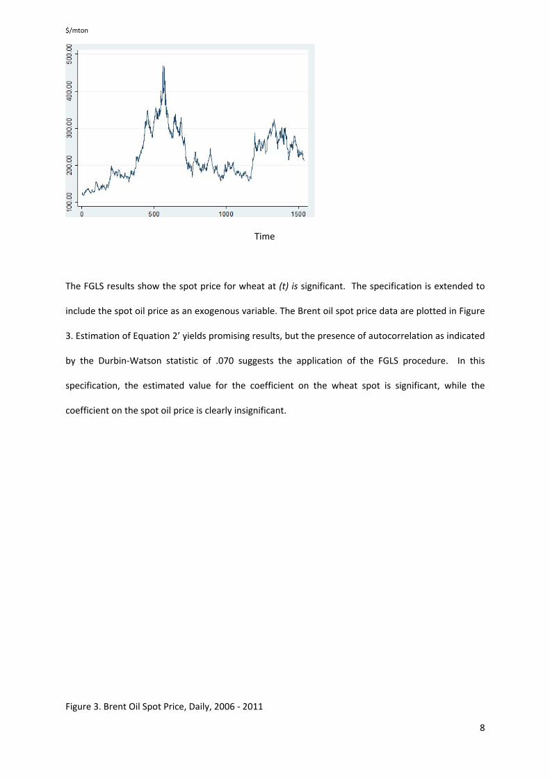
The FGLS results show the spot price for wheat at (t) is significant. The specification is extended to

include the spot oil price as an exogenous variable. The Brent oil spot price data are plotted in Figure

3. Estimation of Equation 2’ yields promising results, but the presence of autocorrelation as indicated

by the Durbin‐Watson statistic of .070 suggests the application of the FGLS procedure. In this

specification, the estimated value for the coefficient on the wheat spot is significant, while the

coefficient on the spot oil price is clearly insignificant.

Figure 3. Brent Oil Spot Price, Daily, 2006 ‐ 2011

9

$/bbl

Time

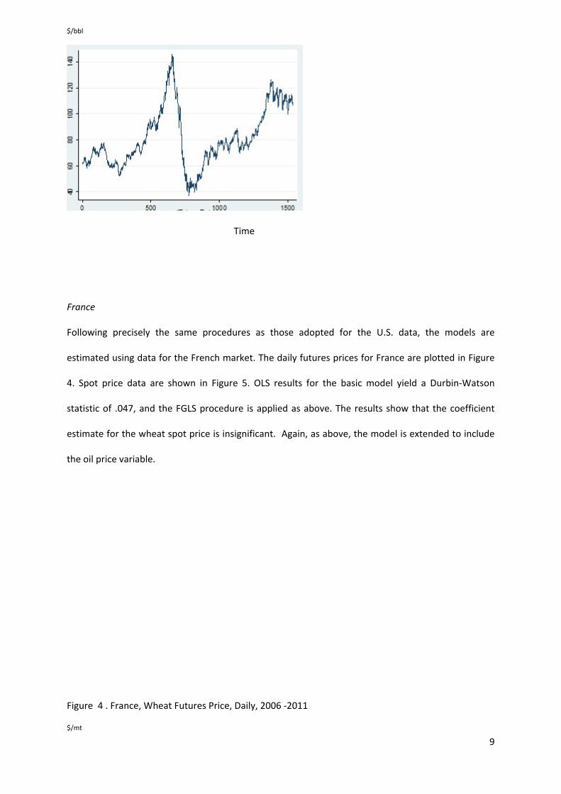
France

Following precisely the same procedures as those adopted for the U.S. data, the models are

estimated using data for the French market. The daily futures prices for France are plotted in Figure

4. Spot price data are shown in Figure 5. OLS results for the basic model yield a Durbin‐Watson

statistic of .047, and the FGLS procedure is applied as above. The results show that the coefficient

estimate for the wheat spot price is insignificant. Again, as above, the model is extended to include

the oil price variable.

Figure 4 . France, Wheat Futures Price, Daily, 2006 ‐2011

$/mt

10

Time

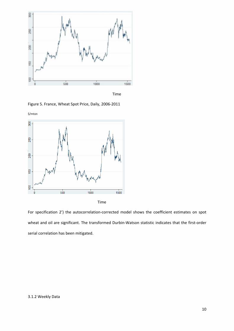
Figure 5. France, Wheat Spot Price, Daily, 2006‐2011

$/mton

Time

For specification 2’) the autocorrelation‐corrected model shows the coefficient estimates on spot

wheat and oil are significant. The transformed Durbin‐Watson statistic indicates that the first‐order

serial correlation has been mitigated.

3.1.2 Weekly Data

11

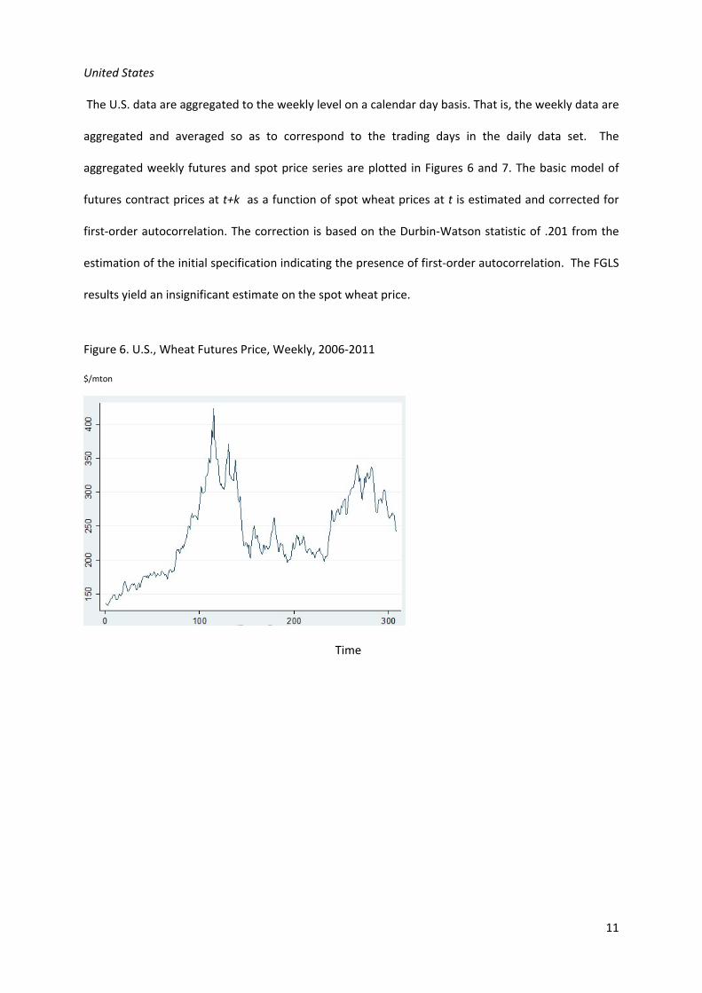
United States

The U.S. data are aggregated to the weekly level on a calendar day basis. That is, the weekly data are

aggregated and averaged so as to correspond to the trading days in the daily data set. The

aggregated weekly futures and spot price series are plotted in Figures 6 and 7. The basic model of

futures contract prices at t+k as a function of spot wheat prices at t is estimated and corrected for

first‐order autocorrelation. The correction is based on the Durbin‐Watson statistic of .201 from the

estimation of the initial specification indicating the presence of first‐order autocorrelation. The FGLS

results yield an insignificant estimate on the spot wheat price.

Figure 6. U.S., Wheat Futures Price, Weekly, 2006‐2011

$/mton

Time

12

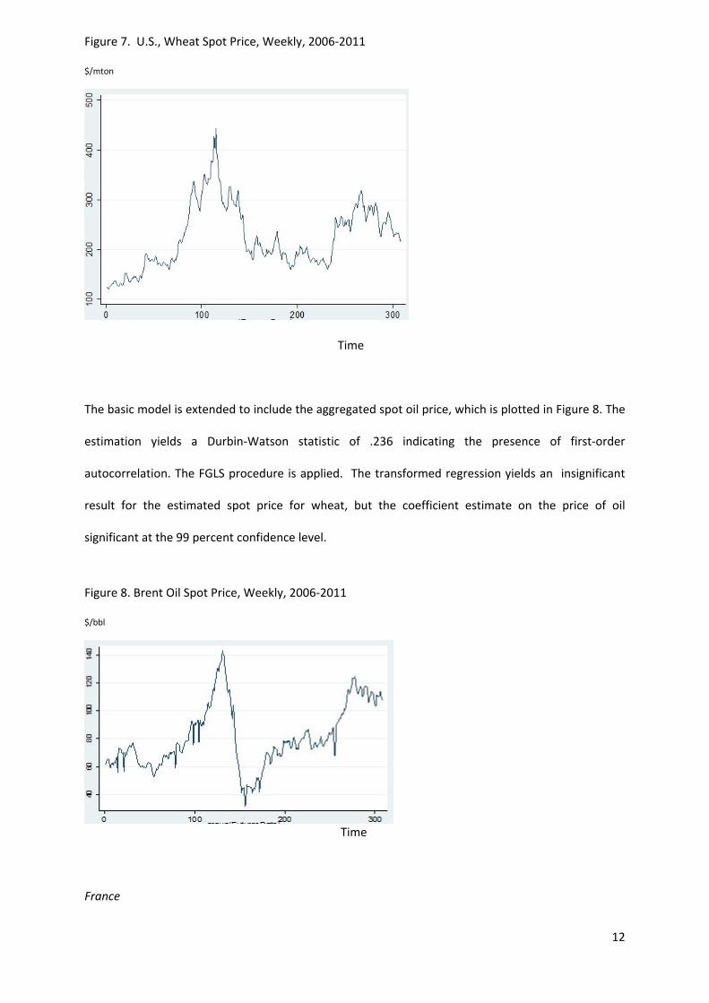
Figure 7. U.S., Wheat Spot Price, Weekly, 2006‐2011

$/mton

Time

The basic model is extended to include the aggregated spot oil price, which is plotted in Figure 8. The

estimation yields a Durbin‐Watson statistic of .236 indicating the presence of first‐order

autocorrelation. The FGLS procedure is applied. The transformed regression yields an insignificant

result for the estimated spot price for wheat, but the coefficient estimate on the price of oil

significant at the 99 percent confidence level.

Figure 8. Brent Oil Spot Price, Weekly, 2006‐2011

$/bbl

Time

France

13

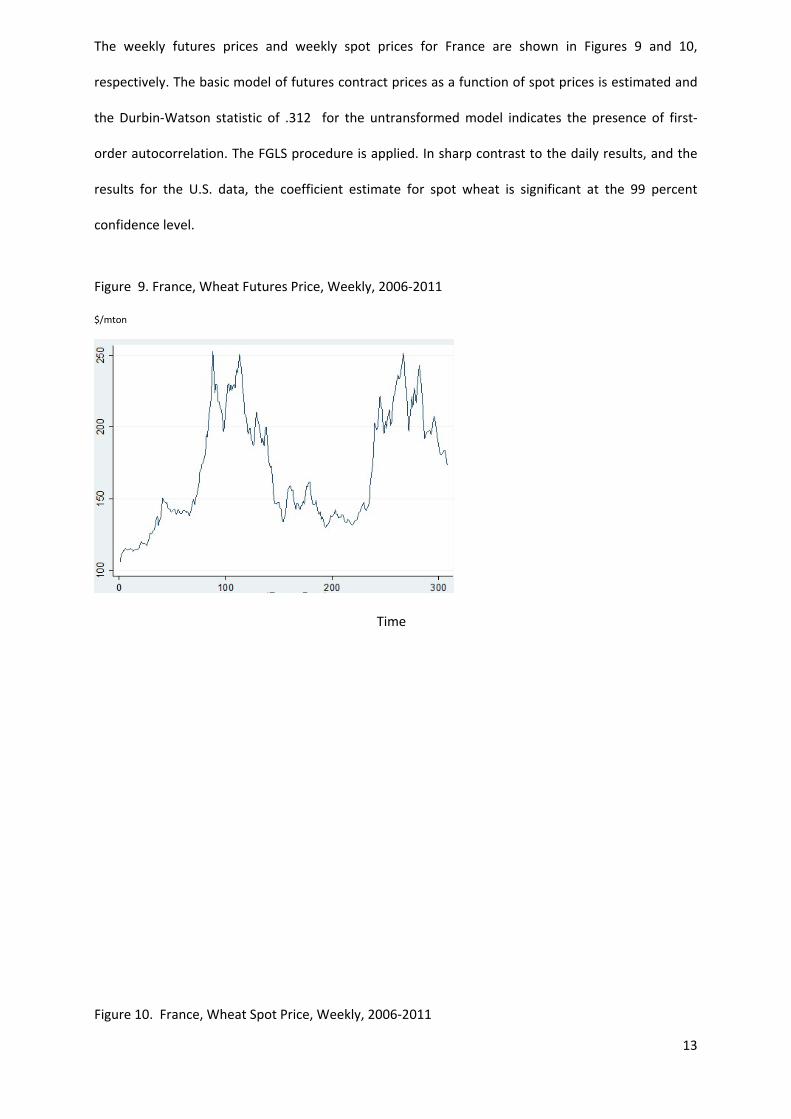
The weekly futures prices and weekly spot prices for France are shown in Figures 9 and 10,

respectively. The basic model of futures contract prices as a function of spot prices is estimated and

the Durbin‐Watson statistic of .312 for the untransformed model indicates the presence of first‐

order autocorrelation. The FGLS procedure is applied. In sharp contrast to the daily results, and the

results for the U.S. data, the coefficient estimate for spot wheat is significant at the 99 percent

confidence level.

Figure 9. France, Wheat Futures Price, Weekly, 2006‐2011

$/mton

Time

Figure 10. France, Wheat Spot Price, Weekly, 2006‐2011

14

$/mt

Time

The model is extended to include the oil price variable. While the initial results from the model

appear promising; the presence of autocorrelation as indicated by the Durbin‐Watson statistic of

.314 suggests application of the FGLS procedure. In contrast to the case using daily data and the U.S.

weekly data, both of the coefficient estimates for the spot price variable and the oil variable are

significant at the 99 percent confidence level. The standard errors of the estimates have also

increased markedly as predicted by theory and shown in Table 1.

3.1.3 Monthly Data

United States

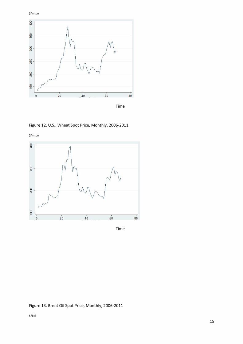
The U.S. monthly futures and spot prices are shown in Figure 11 and Figure 12, respectively. The spot

oil price data are plotted in Figure 13. Estimation of the initial specification indicates first‐order

autocorrelation with the Durbin‐Watson statistic of .841.

Figure 11. U.S., Wheat Futures Price, Monthly, 2006‐2011

15

$/mton

Time

Figure 12. U.S., Wheat Spot Price, Monthly, 2006‐2011

$/mton

Time

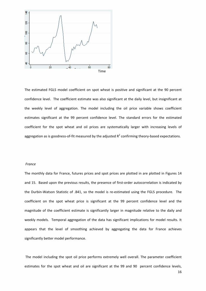
Figure 13. Brent Oil Spot Price, Monthly, 2006‐2011

$/bbl

16

Time

The estimated FGLS model coefficient on spot wheat is positive and significant at the 90 percent

confidence level. The coefficient estimate was also significant at the daily level, but insignificant at

the weekly level of aggregation. The model including the oil price variable shows coefficient

estimates significant at the 99 percent confidence level. The standard errors for the estimated

coefficient for the spot wheat and oil prices are systematically larger with increasing levels of

aggregation as is goodness‐of‐fit measured by the adjusted R2 confirming theory‐based expectations.

France

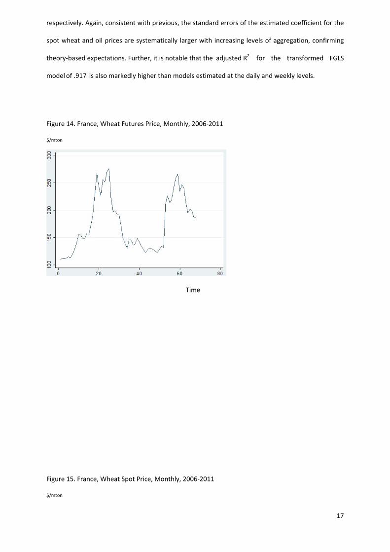
The monthly data for France, futures prices and spot prices are plotted in are plotted in Figures 14

and 15. Based upon the previous results, the presence of first‐order autocorrelation is indicated by

the Durbin‐Watson Statistic of .841, so the model is re‐estimated using the FGLS procedure. The

coefficient on the spot wheat price is significant at the 99 percent confidence level and the

magnitude of the coefficient estimate is significantly larger in magnitude relative to the daily and

weekly models. Temporal aggregation of the data has significant implications for model results. It

appears that the level of smoothing achieved by aggregating the data for France achieves

significantly better model performance.

The model including the spot oil price performs extremely well overall. The parameter coefficient

estimates for the spot wheat and oil are significant at the 99 and 90 percent confidence levels,

17

respectively. Again, consistent with previous, the standard errors of the estimated coefficient for the

spot wheat and oil prices are systematically larger with increasing levels of aggregation, confirming

theory‐based expectations. Further, it is notable that the adjusted R2 for the transformed FGLS

model of .917 is also markedly higher than models estimated at the daily and weekly levels.

Figure 14. France, Wheat Futures Price, Monthly, 2006‐2011

$/mton

Time

Figure 15. France, Wheat Spot Price, Monthly, 2006‐2011

$/mton

18

Time

3.2 Random Coefficient Model

3.2.1 Daily Data

In this section, the data for the U.S. and France are pooled in order to estimate the random

coefficient model as original proposed by Swamy (1970). The algorithm xtrc in STATA is used for this

procedure. It is hypothesized that there exists parameter heterogeneity, which is treated as

stochastic variation. For purposes of this research, the focus is on testing the nonconstancy of

parameters over markets. It might also be on interest to test the model for constancy over time as

well as groups for reasons which are evident based on the time series analysis below. The model as

proposed by Hsiao (1974, 1975) might well be applied in future research. A detailed discussion of the

model can be found in Judge, et al. (1985).

The daily data are as above indicating the use of n=3016 (2 x 1508) covering the periods 2006 – 2011.

Based on the Wald test, the coefficients are jointly significant and the test of parameter constancy as

proposed by Swamy (1970) confirms randomness in the parameter estimates. The coefficient

estimate for the spot oil price is not significant, however. Practically, this result rejects the

homogeneity of the combined or pooled market. That is, under the assumption of one efficient

market, the expectation is that the parameters would be stable indicating market homogeneity.

Given a priori knowledge of the autocorrelation based upon estimation of the single country models,

19

a time trend variable was introduced into the specification. This had marginal effect on the estimates

of the coefficients for spot wheat and oil, but the estimate on the time trend, while small (.010) is

significant at the 99 percent confidence level.

3.2.2 Weekly Data

The weekly aggregated data are as previously indicated and n=608 (2 x304) covering the periods

2006 – 2011. Again, the estimate for the oil spot price is significant. As is the case for the daily data,

for the weekly model, based on the Wald test, the coefficients are jointly significant and the test of

parameter constancy as proposed by Swamy (1970) confirms nonconstancy of the parameter

estimates. While the spot wheat variable is significant 99 percent confidence level the coefficient

estimate for the spot price is not significant. As for the weekly data, a linear time trend variable is

included. Addition of the trend variable does not substantially alter the results recorded without it,

however, the coefficient estimate is significant at the 1 percent significance level.

3.2.3 Daily Data

The monthly aggregated data are as previously indicated and n=134 (2 x 67). The coefficient

estimates are significant at the 90 percent confidence level or better and the results confirm

nonconstancy of the parameters.

The results to this point are summarized in Table 1. To this point, the results suggest a relationship

between the wheat futures price at period t+k and the spot wheat price at period t consistent with

the reverse regression specification. However, this relationship varies considerably with temporal

aggregation. The spot oil price is generally significant across levels of aggregation. These results

certainly seem to confirm the results of Saghaian (2010) that the markets are correlated, but this

does not constitute a claim of causality. Moreover, the temporal aggregation interval is important in

detecting any such relationship. Generally, temporal aggregation results in increased standard errors

on the estimated coefficients and impacts the goodness‐of‐fit. It is noteworthy that there is

20

considerable statistical heterogeneity between the markets, which suggests that even where a

correlation between futures and spot wheat prices is detected, the correlation is not necessarily

stable over the U.S. and French markets.

Table 1. Summary Temporal Aggregation Effects, U.S. and France, 2006-2011*

Daily n=1508 Weekly n=304 Monthly n=68 United States

β δ β δ β δ

Basic Model (FGLS)

.039** (.021)

‐.022 (.050)

.290*** (.093)

Extended Model (FGLS) Adj R2

.039** (.020) .118

.020 (.078)

‐.002 ( .048) .085

.638*** (.117)

.311** (.093)

.211

.715*** (.286)

France

Basic Model (FGLS)

.001 (.021)

.104*** (.046)

.772*** (.030)

Extended Model (FGLS) Adj R2

‐.002 (.021) .046

.032 (.044)

.119*** (.044) .074

‐.154*** (.070)

.760 *** (.029) .812

.125 *** (.067)

Random Coefficient Model (Pooled)

.538 *** (.054)

.897*** (.389)

.632*** (.038)

.681 (.340)

.700*** (.015)

.171 (.174)

*Standard errors are shown below the regression coefficient estimates in parentheses. **Indicates significance at the 10 percent level or better. ***Indicates significance at the 5 percent level or better.

4. Dynamic Models

21

It is well‐known that intertemporal effects in financial models are prevalent. Intertemporal effects

have been recognized at least since the work of Merton (1976) and Black (1976). As these papers

demonstrate the inadequacy of static models, this research extends the results above to estimate a

dynamic formulation of 2’) shown in Equation3.

3) )('')('')('')1('')( ktttsktfktf kk

Where f (t+k‐1) indicates the lagged dependent variable at time t+k‐1. The coefficient 0≥ <1 and

the error term is assumed to have zero expectation and constant variance.

The model is well‐known in economics and finance as a lagged dependent variable (LDV) model, or

more specifically, Equation 3) is a restricted form of the autoregressive distributed lag (ADL) in which

the specification above implies an infinite geometric lag on the variables s(t) and o(t) based upon

application of a Koyck (1954) transformation. A more detailed discussion of the infinite geometric lag

is provided by Judge, Griffiths, Hill, Lütkepohl and Lee (1985).

Based on the results above, there is reason a priori to expect autocorrelation in the residuals giving

rise to issues potentially more complex than those considered in conjunction with the basic model.

This is troublesome as the estimates are likely to be biased and inconsistent. For this reason, an

alternative approach to estimation, GARCH, is applied. Following the work of Engle (2002) and

Bollerslev, Engle, and Nelson (1994), the MGARCH procedure is applied to estimate the parameters

the multivariate generalized autoregressive heteroscedastic model. In this procedure the conditional

variances are modeled as univariate generalized autoregressive conditionally heteroscedastic models

and the covariances are modeled as nonlinear functions of the conditional variances (Engle, 2002). It

is believed that this procedure (STATA mgarch dcc) provides sufficient generality or flexibility for

purposes of this paper. While the models are estimated over alternative levels of aggregation, Drost

and Nijman (1993) have shown that classical GARCH assumptions are not robust to the specification

of the sampling interval. Issues concerning time series modelling of commodity prices, and oil prices

in particular, can be found in the papers by Chen and Lin (2014) and Bopp and Lady (1991).

22

4.1 Daily Data

United States

Applying general procedure for tie series methods, the autocorrelation (ACF) and partial

autocorrelation functions (PACF) for the U.S. futures data are estimated (Granger and Newbold,

1986). The ACF shows significant values at long lags, while PACF exhibits a significant value at lag 1.

The clear indication is that the futures data are non‐stationary and the data first‐differenced. The

first‐differenced series is shown in Figure 16 as an indication of the behavior of the differenced

series. The ACF for the first‐differenced data has a significant value at lag 1 and the PACF decays

rapidly.

Figure 16. First Differences, U.S., Wheat Futures Prices, Daily, 2006‐2011

$/mton

Time

Based on the Phillips‐Perron test for a unit root, the model to be estimated is based on the data

series as in the previous sections, but first differenced. The relationship of interest is the futures price

f k (t+k) as a function of f k (t+k‐1), s (t) and o (t) for each market individually. In order to understand

the empirical relationships between the differenced variables of interest, pairwise Granger (1969)

causality tests. For the U.S., testing variables up to lag 3 gives indications of causal relationships

between the differenced U.S. futures price on the lagged values of the variable itself, as well as weak

23

evidence of causality from the futures variable, the differenced U.S. spot price, and the differenced

oil price variable. There is also considerable evidence of endogeneity amongst the variables of

interest. That is, evidence that the spot wheat and oil prices are at lease contemporaneously related

even if strict causality is not indicated. In particular, there is evidence of strong causality from both

the futures price and the spot price to the differenced oil price.

Using the STATA mgarch dcc algorithm, a GARCH (1, 1) model is estimated. The multivariate dcc‐

GARCH model of Engle (2002) allows the conditional correlations to be time varying. Overall the

model performs reasonably well. The differenced oil price variable is significant. The ARCH and

GARCH terms are significant at any level of confidence. A logarithmic transformation was applied,

but the results indicating persistent heteroscedasticity were not significant altered. This is an

observation to be held for comparison with the models for weekly and monthly data.

To test the ex‐post forecasting accuracy of the U.S. model, the sample is divided into two periods,

estimating the model over the first 1129 observations and holding out the remaining 379

observations for forecasting. The mean squared forecast error for the estimation period is 27.77. The

mean squared forecast error for the hold‐out sample period is 30.08, yielding an in‐sample to hold‐

out ratio of .902.

France

The procedures applied to the U.S. daily data are followed precisely using the data for France. As

above based on the ACF and PACF for the data series on the prices for futures contracts, the data are

first differenced. The results for the Phillips‐Perron test for a unit root suggest estimation with first

differences of the series for France, although differences of logarithms might also be considered.

Based on the Granger causality tests, it appears that the differenced futures series is caused by the

lagged values of itself the differenced spot price series, but not the differenced oil price series.

There is considerable causality as between the differenced spot price, the futures price variables

and the difference oil price. Despite some ambiguity in the choice of transformation, the GARCH (1,

24

1) specification is estimated. As reported in Table 2, excepting for the ARCH and GARCH terms, the

model has very little explanatory power at least as a consequence of inclusion of the lagged futures

price spot price and oil variables.

As in the previous subsection, in order to test the forecasting accuracy of the model, the sample is

divided into two periods; the first 1127 observations and holding out the remaining 381 observations

for ex‐post forecasting. Reestimation of the model over the indicated sample period does yield a

coefficient estimate on spot oil significant at the 95 percent confidence level. The mean squared

forecast error for the estimation period is 6.25. The mean squared forecast error for the hold‐out

sample period is 15.03, yielding an in‐sample to out‐of‐sample mean squared error ratio of ratio of

.416. The result is not unusual given the generally poor performance of the model.

4.2 Weekly Data

United States

The weekly aggregated time series data for the U.S. have an ACF which decays slowly and becomes

insignificant only at long lags. The PACF shows a significant values at lag 1. The series clearly

indicates significant heteroscedasticity. The Peron‐Philips test for a unit root indicates estimation

with the first‐differenced series shown in Figure 17.

Figure 17. First‐Differences, U.S., Wheat Futures Prices, Weekly, 2006‐2011

$/mton

25

Time

The Granger causality tests are run for the differenced futures price, the futures price lagged 1

period, the spot price and the oil price variable. The results indicate that the differenced futures price

is Granger‐caused by its own lagged value as well as the differenced spot wheat price and the

differenced spot oil price. Further, There is evidence that the differenced futures price, the

differenced spot wheat price and differenced spot oil price is Granger caused by the other variables

under consideration. Thus, as expected, endogeneity is an issue.

A GARCH (1, 1) model is estimated using the weekly U.S. data. The model seems to perform quite

well relative to the daily model with the exception of the pronounced period of variation between

periods 100 and 150. In order to test the forecasting accuracy of the model, the first 226

observations are used for estimation and the remaining 78 observations are used to test one‐step

ahead forecasting accuracy. The mean squared error of the forecasts over the estimation period is

95.19. Interestingly, and owing to the volatility toward the end of the estimation period, the mean‐

squared forecast error for the hold‐out period is 78.05 resulting in the in‐sample to out‐of‐sample

error ratio of 1.22.

France

26

The weekly aggregated time series data for France have an ACF which decays and becomes

insignificant at long lags. The PACF shows two significant values at lags 1 and 2. On the basis of this

result and the Phillips‐Perron test, first differences of the series are used for estimation purposes.

The results from the Granger causality tests are consistent with findings reported for the U.S. weekly

data. The GARCH (1, 1) specification is applied to the weekly French data. That is, while there is

indication of causality from the differenced lagged futures, spot and oil prices, the reverse is also

indicated. In order to test the forecasting accuracy of the weekly model, the first 226 observations

are used for estimation purposes and one‐step ahead forecasts are generated for the remaining 78

observations. The mean squared forecast error for the in‐sample estimation is 29.46. The mean

squared forecast error for the out‐of‐sample horizon is 50.75. The in‐sample to out‐of‐sample mean

squared error ratio is .580.

4.3 Monthly Data

United States

The time series are applied to the monthly U.S. data. Based on the patterns of the ACF and PACF for

the data series on the prices for futures contracts, the data are first differenced. The first‐

differenced series for the U.S. is shown in Figure 18. The ACF and PACF both show significant values

at lag 1 and decay rapidly according to a sinusoidal pattern. Consistent with previous findings, the

data series show causality from the differenced and lagged futures, spot and oil variables, but there

is also pronounced evidence of two‐way causal relationships.

27

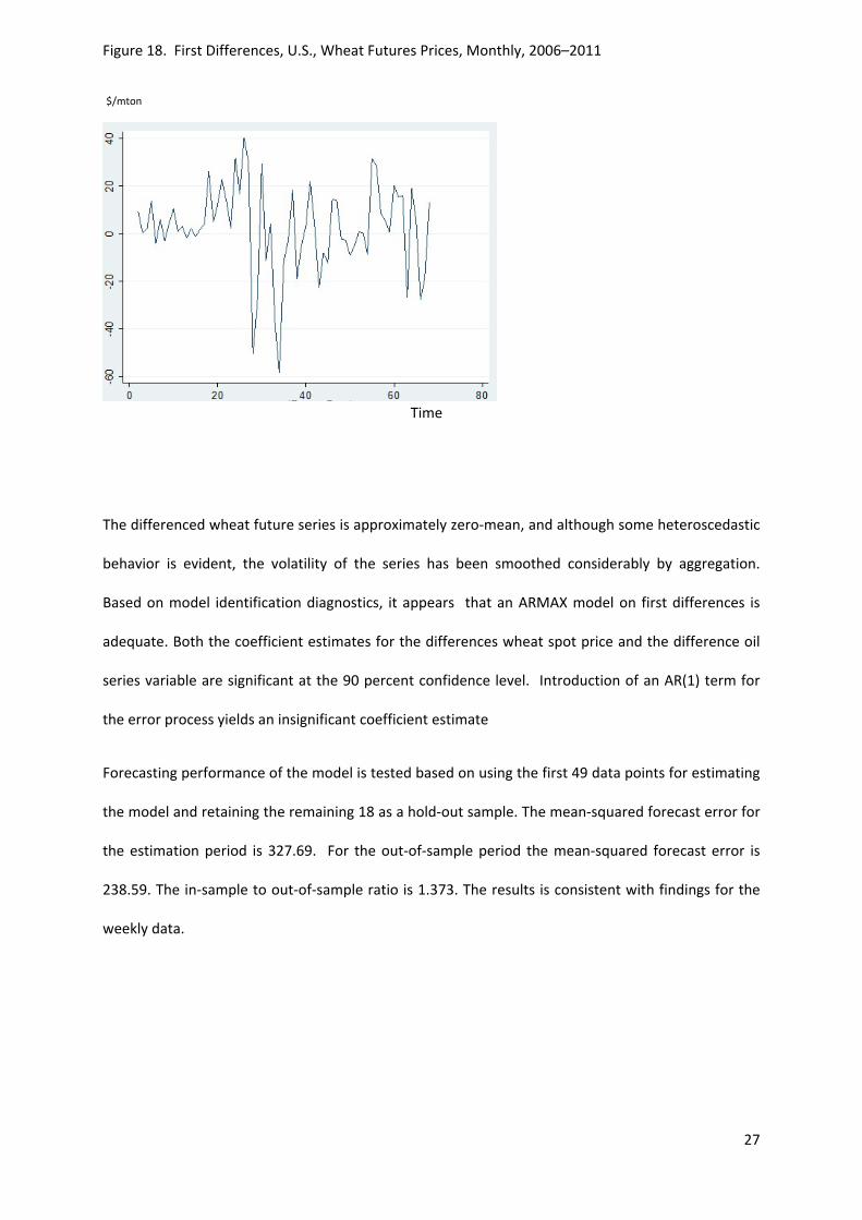
Figure 18. First Differences, U.S., Wheat Futures Prices, Monthly, 2006–2011

$/mton

Time

The differenced wheat future series is approximately zero‐mean, and although some heteroscedastic

behavior is evident, the volatility of the series has been smoothed considerably by aggregation.

Based on model identification diagnostics, it appears that an ARMAX model on first differences is

adequate. Both the coefficient estimates for the differences wheat spot price and the difference oil

series variable are significant at the 90 percent confidence level. Introduction of an AR(1) term for

the error process yields an insignificant coefficient estimate

Forecasting performance of the model is tested based on using the first 49 data points for estimating

the model and retaining the remaining 18 as a hold‐out sample. The mean‐squared forecast error for

the estimation period is 327.69. For the out‐of‐sample period the mean‐squared forecast error is

238.59. The in‐sample to out‐of‐sample ratio is 1.373. The results is consistent with findings for the

weekly data.

28

France

Applying the time series procedures to the monthly data for France yields an ACF which exhibits a

sinusoidal pattern with the estimated values decreasing at increasing lags. The PACF exhibits a

significant value at lag 1. Diagnostic checks indicate first‐differencing of the data series. Testing the

series for the presence of a unit root suggests the series is stationary.

Granger causality tests estimated on the pairwise basis show evidence of two‐way causality between

the differenced spot price and the differenced futures price. There is also significant evidence of

causality from the differenced wheat futures and spot price to the differenced oil price. As with the

U.S. data, model identification is somewhat problematic, but it appears as though the ARMAX

specification with and AR(1) error term is adequate. It is somewhat surprising that the coefficient

estimate on the differenced spot price is negative and significant.

In order to compare the model with other time series specifications on the basis of forecast error,

the monthly model is estimated using the first 49 data periods and the remaining 18 are used for ex‐

post forecasting. The in‐sample mean squared forecast error is 17.93. The one‐step ahead forecasts

are generated for the 17 observations of the hold‐out sample. The mean squared forecast error for

the one‐step ahead forecasts over the hold‐out sample is 110.08, yielding an in‐sample to out‐of‐

sample ratio of .163. Thus, the ratio is considerably smaller than the daily or weekly ratios. The poor

out‐of‐sample performance is due to very large prediction errors in periods 58, 59 and 62.

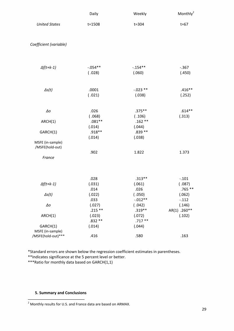
The results from estimation of the dynamic models is shown in Table 2. The sample sizes for the

daily, weekly and monthly modes are 1538, 308 and 68, respectively. The symbol Δ denotes first‐

difference of the series. These results show standard errors of the coefficients increasing with

aggregation levels. In terms of forecasting performance, the results are ambiguous. For the U.S.

models out‐of‐sample squared forecast error is greater that in‐sample squared error, but in sample

squared error exceeds out‐of‐sample for the weekly and monthly models. For France, the data

exhibit different behaviors at different levels of aggregation. This is consistently with the findings of

Drost and Nijman (1993).

Table 2 . Summary Temporal Aggregation Effects, GARCH (n, p) U.S. and France, 2006‐2011

29

Daily Weekly Monthly2

United States t=1508 t=304 t=67

Coefficient (variable)

Δf(t+k‐1) ‐.054** ( .028)

‐.154** (.060)

‐.367 (.450)

Δs(t) .0001 ( .021)

‐.023 ** (.038)

.416** (.252)

Δo .026 ( .068)

.375** ( .106)

.614** (.313)

ARCH(1) .081** (.014)

.162 ** (.044)

GARCH(1) .918** (.014)

.839 ** (.038)

MSFE (in‐sample) /MSFE(hold‐out)

.902 1.822 1.373 France

Δf(t+k‐1)

.028

(.031) .313** (.061)

‐.101 ( .087)

Δs(t) .014

(.022) .026

( .050) .765 ** (.062)

Δo .033

(.027) ‐.012**

( .042) ‐.112

(.146)

ARCH(1) .215 **

(.023) .319** (.072)

AR(1) .260** (.102)

GARCH(1) .832 ** (.014)

.717 ** (.044)

MSFE (in‐sample) /MSFE(hold‐out)*** .416 .580 .163

*Standard errors are shown below the regression coefficient estimates in parentheses. **Indicates significance at the 5 percent level or better. ***Ratio for monthly data based on GARCH(1,1)

5. Summary and Conclusions

2 Monthly results for U.S. and France data are based on ARMAX.

30

This paper analyzes empirically the possible relationship between wheat futures prices and spot oil

prices as well as the effects of temporal aggregation on the specification of alternative models of

wheat futures contract prices, and consequently, on the understanding of the empirical relationship

between the two markets (e.g., wheat and oil). Alternative models have been specified and tested.

Key observations from this research include the fact that the wheat futures price and the spot oil

prices are correlated as pointed out by Saghaian (2010). The fact that the random coefficient model

leads to the rejection of the null hypothesis of parameter constancy does bring into question the

stability of that correlation, however.

As to causality is seems clear that temporal aggregation does impact the relationships between the

variables as well as the model coefficient estimates, standard errors and forecasting accuracy. With

respect to coefficient estimates and the associated standard errors, consistent with theory, standard

errors tend to increase with the level of aggregation, so there are coincident implications for

accuracy and inference. Forecast accuracy is also impacted by aggregation, although in the context

of this paper, the results are mixed as concerns relative accuracy as measured by ratios of mean

squared forecast errors using selected periods for model estimation and computing one‐step ahead

forecast for a hold‐out sample. The hypothesis that the monthly unit of aggregation is “optimal”

based upon supply chain dynamics relating energy markets to food commodity prices does not find

unequivocal support in this research suggesting future research

As concerns market homogeneity, at least for the specification tested in this research, it appears that

conventional ordinary least squares (OLS) models using pooled data will be misspecified owing to

nonconstancy of the parameter estimates indicated by application of the Swamy (1970) random

coefficient model. Finally, consideration of a dynamic specification confirms the importance of

intertemporal effects.

31

From a practical perspective, it is clear that so‐call reverse regressions can be useful for

understanding and predicting prices of futures contracts and the relationship, contemporaneous and

causal, to other markets. However, the degree or significance of the relationship varies and

awareness of the effects of temporal aggregation are required owing to the deterioration of

coefficient estimates as aggregation increases. Such aggregation effects impact understanding the

relationship between markets. With respect to forecasting, this research points clearly toward the

importance of using historical data to test forecast accuracy for specific series at alternative

aggregation levels before generating out‐of‐sample predictions. As concerns future research, the

authors intend to extend the analysis with respect to methodology by applying the approach taken in

this paper to understanding the relationships between other energy prices and those of other food

commodities.

REFERENCES

Baffles, J. (2007), “Oil Spills on Other Commodities”, Resources Policy, 32, pp. 126‐134.

Black, S. (1976), “Rational Response to Shocks in a Dynamic Model of Capital Asset Pricing,” American Economic Review, 66, pp. 767‐779.

Bollerslev, T., Engle, R.F. and Nelson, DB. (1994), “ARCH Models”, in Handbook of Econometrics; Volume IV, ed. R.F. Engle and D.L. McFadden, New York: Elsevier.

Campbell, J.Y. and Shiller, R.S. (1987), “Cointegration and Tests of Present Value Models”, Journal of Political Economy, 95 (5), pp. 1062‐1088.

Cartwright, P. and Lee C.F. (1987), “Time Aggregation and the Estimation of the Market Model: Empirical Evidence”, Journal of Economic and Business Statistics, 5, pp. 131‐143.

Chen, S.W. and Lin, S.M. (2013), “Non‐linear Dynamics in International Resource Markets: Evidence from Regime Switching Approach”, Research in International Business and Finance, 30, pp. 233‐247. Chen, Y., Rogoff, K. and Rossi, B. (2008), “Can Exchange Rates Forecast Commodity Prices?”, National Bureaus of Economic Research, Working Paper 13901. Dornbusch, R. (1976), “Expectations and Exchange Rate Dynamics,” Journal of Political Economy, December, pp. 1161‐1176.

Drost, F.C. and Nijman, T.E. (1993), “Temporal Aggregation of GARCH Processes,” Econometrica, 61, pp. 909‐927.

32

Durbin, J.C. (1970), “Testing for Serial Correlation in Least Squares Regressions When Some of the Regressors are Lagged Dependent Variables”, Econometrica, 38, pp. 410‐421.

Engel, C. and West, K.D. (2005), “Exchange Rates and Fundamentals”, Journal of Political Economy, 113, pp. 485‐517. Engle, R.F. (2002), “Dynamic Conditional Correlation: A Simple Class of Multivariate Generalized Autoregressive Conditional Heteroscedasticity Models”, Journal of Business and Economic Statistics,20, pp. 339‐350. Engle, R.F. and Liu, T.C. (1972), "Effects of Aggregation Over Time on Dynamic Characteristics of an Econometric Model", pp.673‐728, in Econometric Models of Cyclical Behaviour, ed. B.G.Hickman New York: Columbia University Press. Granger, C.W.J. and Newbold, P. (1986), Forecasting Economic Time Series, 2nd ed., London: Academic Press. Granger, C.W.J. (1969). "Investigating Causal Relations by Econometric Models and Cross‐spectral Methods". Econometrica 37 (3), pp. 424–438. Hsiao, C. (1974), “Statistical Inference for a Model with both Random and Cross‐Sectional and Time Series Effects”, International Economic Review, 15, pp. 12‐30. Hsiao, C. (1975), “Some Estimation Methods for a Random Coefficient Model”, Econometrica, 43, pp. 305‐325. Index Mundi (2013), “Crude Net Balance by Country, 2009”. Available at

http://www.indexmundi.com/blog/index.php/2013/05/03/crude‐oil‐exports‐and‐imports‐by‐country/ International Grains Council (2013), Information Services. Available at http://www.igc.int. Accessed November 1, 2013. Judge, G.G., Griffith, W.E., Hill, R.C., Lütkepohl, H. and Lee, T.C. (1985), The Theory and Practice of Econometrics, 2nd edition, New York: John Wiley. Knittel, C.R. and Pindyck, R. (2013), “The simple Economics of Commodity Price Speculation”, MIT Center for Energy and Environmental Policy Research, CEEPR WP 2013‐06. Koyck, L. M. (1954), Distributed Lags and Investment Analysis, Amsterdam: North‐Holland. Marcellino, M. (1999), “Some Consequences of Temporal Aggregation in Empirical Analysis”, Journal of Business and Economic Statistics, 17, 1, pp. 129‐136. Merton, R.C. (1976), “An Intertemporal Capital Asset Pricing Model”, Econometrica, 41, pp. 867‐887. Muhammed, A. and Kebede, E. (2009), “The Emergence of an Agro‐Energy Sector: Is Agriculture Importing Instability from the Oil Sector?”, Choices, 24, 1, pp. 12‐15. Pindyck, R. (2001), “Dynamics of Commodity Spot and Futures Markets: A Primer”, The Energy Journal, 22, 3, pp. 1‐29. Posner, R. (2013), “Commodity Price Fluctuations‐Posner”, The Becker‐Posner Blog. August 4, 2013. Available at http://www.becker‐posner‐blog.com/2013/08/commodity‐price‐fluctuationsposner.html. Accessed July 23, 2013.

33

Prais, S. J., and Winsten, C.B. (1954). “Trend estimators and serial correlation”. Working paper 383, Cowles Commission. Available at http://cowles.econ.yale.edu/P/ccdp/st/s‐0383.pdf. Accessed October 15, 2013. Roberts, M.J. and Schlenker, W. (2013), “Identifying Supply and Demand Elasticties of Agricultural Commodities: Implications for the US Ethanol Mandate”, The American Economic Review, 103, 6, pp. 2265‐2295. Robledo, C.W. (2002), Dynamic Econometric Modeling of the U.S. Wheat Grain Market, Ph.D. Dissertation, The Department of Agricultural Economics and Agribusiness, Louisiana State University and Agricultural and Mechanical College. Roll, R. (1984), “Orange Juice and the Weather”, American Economic Review, 74, pp. 861‐880. Rowe, R. (1976), “The Effects of Temporal Aggregation Over Time on T‐Ratios and R2’s”, International Economic Review, 17, pp. 751‐757.

Saghaian, S. H. (2010), “The imt of the Oil Sector on Commodity Prices: Correlation or Causation”, Journal of Agricultural and Applied Economics, 42, 3, pp. 477‐485.

Silvestrini, A. and Veredas, D. ( 2005), "Temporal Aggregation of Univariate Linear Time Series

Models”, Core Discussion Papers 2005059, Université catholique de Louvain, Center for Operations

Research and Econometrics (CORE).

Slate Magazine (2012, “Agricultural Exports and Imports”. Available at http://www.slate.com/articles/technology/future_tense/2012/06/a_map_of_farmers_in_the_u_s_and_world_.html. STATA, Longitudinal Data/Panel Data, Release 12 (1985‐2011), College Station: Stata Press. STATA, Time Series, Release 12 (1985‐2011), College Station: Stata Press. Swamy, P.A.V.B. (1970), “Efficient Inference in a Random Coefficient Regression Model”, Econometrica, 38, pp. 311‐ 323. Woertz, E. (2013), “Oil For Food: Big Business in the Middle East”, The World Financial Review. Available at http://www.worldfinancialreview.com/?p=2773. Accessed October 23, 2013. Zellner, A. and Montmarquette, C. (1971), “A Study of Some Aspects of Temporal Aggregation Problems in Economics and Statistics”, The Review of Economics and Statistics, 53, pp. 335‐342.

Measuring the Effect of Oil Prices on Wheat Futures Prices

Documents

Transcript of Measuring the Effect of Oil Prices on Wheat Futures Prices