Deregulation of wholesale petrol prices: what happened to capital city petrol prices

Deregulation of wholesale petrol prices: whathappened to capital city petrol prices?

Alistair Davey†

Wholesale petrol prices were deregulated in August 1998. This paper will quantify theeffect associated with the deregulation of wholesale petrol prices on relative retailprices for unleaded petrol in Adelaide, Melbourne and Sydney. This is done throughBox–Jenkins autoregressive integrated moving average methodology coupled withBox and Tiao intervention analysis. Weekly price data will be used for Adelaide,Melbourne, and Sydney. It finds that from the beginning of 1999, deregulationcoincided with relatively lower retail petrol prices for all three cities. In the absence ofany other possible alternative explanation for the simultaneous fall in relative retailpetrol prices across all three cities, it is concluded that this change was most likelyassociated with deregulation. These results suggest that regulation of wholesale petrolprices were ineffectual in terms of constraining capital city retail petrol prices at thevery least and may have actually contributed towards relatively higher retail petrolprices. This also suggests that future policy interventions designed to constrain pricesin the downstream petroleum industry should be very carefully considered.

Key words: competition, deregulation, petrol prices.

1. Introduction

Wholesale petrol prices were subject to either price control or price surveil-lance mechanisms by either the Commonwealth or state governments fromFebruary 1940 until July 1998. The regulation was usually justified over con-cern about the degree of effective competition in the downstream petroleumindustry and the need to protect against monopolistic pricing (Royal Com-mission on Petroleum 1976, p. 347). The regulation had generally been basedon setting a maximum wholesale price calculated by a formula estimating thecost of importing fuel to the Australian seaboard and the associated costs ofdistribution. However, in July 1998, the Commonwealth Governmentannounced that it was deregulating wholesale petrol prices from the begin-ning of August 1998 (Costello and Moore 1998).The only previous study of deregulation came to a negative assessment of

its consequences. Based on a partial adjustment model comparing wholesalepetrol prices during a period of regulation to a period following deregulation,Delpachitra and Beal (2002) concluded that deregulation had benefited oilcompanies more than consumers and had not increased price competition.

†Alistair Davey (email: [email protected]), is Senior Consultant with ACILTasman, Canberra, Australia.

� 2010 The AuthorJournal compilation � 2010 Australian Agricultural and Resource Economics Society Inc. and Blackwell Publishing Asia Pty Ltddoi: 10.1111/j.1467-8489.2009.00480.x

The Australian Journal of Agricultural and Resource Economics, 54, pp. 81–98

The Australian Journal of

Journal of the AustralianAgricultural and ResourceEconomics Society

The purpose of this paper is to quantify the impact of deregulation on rela-tive retail prices for unleaded petrol in Adelaide, Melbourne and Sydney.This will be investigated through a time series or before-and-after analysiswith any difference in relative retail petrol prices before and after deregula-tion being interpreted as the effect of the policy change.The structure of this paper is as follows. Section 2 will provide a brief out-

line of the downstream petroleum industry in Australia in capital cities.Section 3 describes the data to be used in this study. Section 4 will provide themodel specification. Section 5 will present the results and Section 6 willprovide the conclusions.

2. Australian downstream petroleum industry

The Australian downstream petroleum industry is dominated by fourvertically integrated companies that operate in oil refining, petroleum prod-uct distribution and wholesale, and retailing sectors: Caltex, BP, Mobil andShell (collectively known as the oil majors). The oil majors operate whollyowned wholesale or distribution companies separate from their refiningoperations through which they distribute petrol to retailers. The oil majors’distribution companies typically supply their own branded retail servicestation networks as well as other metropolitan area customers. In 2000,around 90 per cent of retail service stations were part of branded networks ofthe oil majors (Australian Institute of Petroleum 2006, p. 18).To gain access to petrol supply in states where they did not possess a refin-

ery, the oil majors used supply swap arrangements known as refineryexchange agreements (REAs) where product was exchanged between them ona litre-for-litre basis. While this enabled the oil majors to save on transporta-tion costs, the Australian Competition and Consumer Commission (ACCC)(1996, p. 31) opined that REAs ‘may have potentially anti-competitiveeffects’. In January 2000, REAs for the Mobil Port Stanvac refinery nearAdelaide were terminated although they remained in place for other cities(Cummins 1999).An independent refers to market participants that are not vertically inte-

grated from refining to retailing, although they are sometimes reliant on oilmajors for fuel supply. Despite accounting for less than 10 per cent of retailservice stations throughout Australia, independent retailers have traditionallyhad a stronger presence within capital cities. In 1996, the ACCC (1996, p. 77)observed that independent retailers imposed a significant competitive con-straint on the oil majors’ retail petrol pricing.Given the absence of an independently operated fuel import terminal in

Adelaide, independent petrol wholesalers and retailers were entirely depen-dent on supply from the oil majors to sustain their operations. However,independently operated fuel import terminals near Melbourne and in Sydneycould supply independent wholesalers and retailers with imported fuel. In1996, the ACCC (1996, p. 57) expressed optimism regarding the ongoing

82 A. Davey

� 2010 The AuthorJournal compilation � 2010 Australian Agricultural and Resource Economics Society Inc. and Blackwell Publishing Asia Pty Ltd

capacity of independent petrol imports to impose a competitive constraint onthe oil majors.Within major capital cities, the ACCC (1996, p. 77) has observed there are

regular retail petrol price cycles. These price cycles generally follow a recur-ring sawtooth pattern where prices rise rapidly and then steadily decreaseover time (ACCC 2005, p. 6).There are several different types of retail service stations operating in

Australia’s capital cities:

• Company operated stations.• Commission agent stations that sell branded petrol at prices set by theirfuel supplier with the operator receiving a fixed commission on petrol sales.

• Franchise stations where the franchisee has a contractual agreement with afranchisor. The majority of sites owned by the oil majors during this studywere operated through franchise agreements.

• Dealer-owned stations where the operator has an agreement with a sup-plier to carry a supplier’s brand.

If the oil major were able to exercise any market power at the wholesalelevel, then it would reduce their profitability to have franchised service sta-tions also exercising market power as double marginalisation would occur.Double marginalisation occurs wherever market power is exercised at succes-sive vertical stages of production. For example, with petrol, if market poweris exercised at the distribution and wholesale level and then again at the retaillevel, the petrol wholesaler will mark up the product and the petrol retailerwill then take the wholesale price and mark it up again. This double mark-upresults in lower total sales and lower total profit than if wholesaler and retai-ler were vertically integrated.To avoid double marginalisation, Rose (1999, pp. 18–19) argued the oil

majors seek to maximise competition among firms operating at the retail levelthrough utilising multiple sources of distribution such as franchisees, com-pany-owned sites, commission agent sites and independents. This is consis-tent with the observations of Roarty and Barber (2004) that petrol retailing isa low-margin business.To prevent double marginalisation, the oil majors are probably forcing the

retail petrol price down to marginal cost. On this basis, competition withinretail petrol markets would approximate perfect competition where price isequated to marginal cost. If petrol is retailed at marginal cost, then retail pet-rol prices should convey information regarding the interactions of partici-pants in wholesale petrol markets and should closely follow and reflectchanges in wholesale petrol prices.

3. Data construction

To undertake a direct analysis of any price effect associated with deregulationwould require wholesale price data both before and after deregulation.

Deregulation of wholesale petrol prices 83


However, wholesale price data is not generally available because of high com-mercial sensitivity (Delpachitra and Beal 2002, p. 60).This arguably leaves the retail price as the only other price indicator

available to undertake the analysis. As concluded in Section 2, if petrol isretailed at marginal cost, then prices should closely follow and reflect changesin wholesale prices. Unlike wholesale prices, retail prices are publiclyavailable information. Therefore, deregulation will be tested through its effecton the retail price of regular unleaded petrol sold in Adelaide, Melbourneand Sydney. Provided all other things are equal (the ceteris paribusassumption), the effect of deregulation on wholesale petrol markets inAdelaide, Melbourne and Sydney should be measurable through changes inretail petrol prices.However, the ceteris paribus assumption is often violated as retail petrol

prices are subject to influences aside from structural change affecting capitalcity wholesale petrol markets. These other influences include the internationalcrude oil price, which is the major input into petrol production, and refiningmargins, the difference between refined petroleum product prices and crudeoil prices.To extricate these other influences from the retail petrol price, a notional

industry margin (NIM) has been constructed by subtracting a proxy for thewholesale petrol price unaffected by developments in Australian wholesalepetrol markets from the retail petrol price. The NIM estimates the totalnotional margin accruing to petrol suppliers at various stages in the supplychain. Thus, assuming that petrol is retailed at marginal cost, the level of theNIM should reflect developments and changes in capital city wholesale mar-ket conditions and generally provide an indication of the returns accruing tothe oil majors.Weekly average retail unleaded petrol price data (RP) was obtained from

market research company Informed Sources. The proxy used for the whole-sale unleaded petrol price was the import parity indicator price (IPI) calcu-lated by the ACCC.1 The IPI was the instrument used by the ACCC to set themaximum wholesale petrol price under regulation. The calculation of the IPIis composed of three components:

• The import parity component – the ‘landed cost’ for ex-refinery petrolstock from Singapore (incorporating the spot price for fuel, freight,wharfage, insurance and loss, and the Australian/US dollar exchangerate);

• The assessed local component – reflecting influences such as downstreamterminalling, marketing and distribution costs as well as return on assetsemployed in that sector; and

• Excise and state subsidies, and the goods and services tax (GST) (ACCC2001, p. 10).

1 The IPI was provided to the researcher by the ACCC on a confidential basis.

84 A. Davey


Singapore is considered the appropriate benchmark for Australian petrolprices as it is the closest major refining and marketing centre and the mostcommon source for imported petrol.An adjustment was made to the IPI to remove the local component

because, more often than not, the NIM calculated from an IPI including thelocal component was negative. Persistent ongoing negative NIM observationsare a perverse result, as firms cannot continue in business indefinitely if theycannot cover their costs. This suggests the local component of the IPI, thatwas 7.1 cents per litre (cpl), had probably been set too high. Rather thanhaving a data series consisting largely of negative NIM observations, it wasconsidered preferable to remove the local component from the IPI. Removal,however, does not change the relativities between the NIM observations.The Commonwealth Government levies an excise tax on petrol sales, set at

a particular rate in cpl. Responsibility for paying the excise rests withrefiners.2 Refiners pass the cost of the excise on to buyers of petrol, so thatthe excise is eventually passed on to consumers. Because petrol excise isapplied on the basis of a fixed amount, the excise applying to both the IPIand the RP is the same. Consequently, in calculating the NIM, the impact ofpetrol excise is removed when subtracting the IPI from the RP.The Commonwealth Government introduced a GST on 1 July 2000 which

applied to petrol. The GST is an ad valorem tax set at 10 per cent. Because theGST is applied to each transaction in a supply chain on an ad valorem basis,any difference between the IPI and the RP will result in a discrepancy in theamount of GST applying to the IPI when compared with the RP. Becausethe amount of GST applying to the IPI and the RP could differ, the level ofthe NIM could either increase or decrease directly as a result of the imposi-tion of the GST, thus resulting in a distortion in the estimation of the NIM.An adjustment was made to both the IPI and the RP to remove the GSTimpact on the NIM.Until August 1997, all state governments except Queensland levied busi-

ness franchise fees on the sale of petrol. In New South Wales, Victoria andSouth Australia, the petrol franchise fee was levied in two parts. The first partwas a flat nominal fee imposed on retailers who purchased their petrol from alicensed wholesaler (Gabbitas and Eldridge 1998, p. 231). The second partwas a fee payable as a given percentage of the declared value – in this case theprice in cpl as determined by the state government (Gabbitas and Eldridge1998, p. 231). The variable component of the petrol franchise fee applying inSydney in 1997 was 7.88 cpl, in Melbourne it was 9.28 cpl at the start of 1997and fell to 7.67 cpl on 1 June 1997 and in Adelaide it was 9.77 cpl at the begin-ning of the year and rose to 9.85 cpl on 1 July 1997 (Australian Institute ofPetroleum 1998).On 5 August 1997, a High Court ruling on the legality of tobacco business

franchise fees in New South Wales cast doubt on the constitutional validity

2 Customs duty is levied on comparable imports at the same rate.



of petrol franchise fees. Consequently, all state governments ceased their col-lection. On 6 August 1997, the Commonwealth Government announcedsafety net arrangements whereby it would increase the rate of petrol exciselevied and return the revenue collected to the states.Each state had set a different level for its petrol franchise fee, but because

the Commonwealth Government is unable to discriminate between statesunder the Constitution, the Commonwealth Government increased its exciserate by 8.1 cpl across the board. A condition of the Commonwealth Govern-ment’s safety net arrangements was that petrol prices not increase because ofthis arrangement. To meet this condition, the New South Wales Governmentprovided an interim subsidy of 0.22 cpl to petrol wholesalers from August1997 until November 1997 and the Victorian Government provided a subsidyof 0.43 cpl to petrol wholesalers from August 1997 until July 2007.To account for the period in which petrol franchise fees applied, the rele-

vant amount of the variable rate of the petrol franchise fee applying in eachcity has been added to the IPI (as the IPI was provided exclusive of petrolfranchise fees). To account for the interim subsidies, 0.22 cpl has been sub-tracted from the IPI for Sydney between August and November 1997, and0.43 cpl has been subtracted from the IPI in Melbourne from August 1997onwards, rising to 0.473 from July 2000 to account for the imposition of theGST.After the adjustments described were made, the NIM was estimated

through the following equation:

NIM ¼ RP� IPI ð1Þ

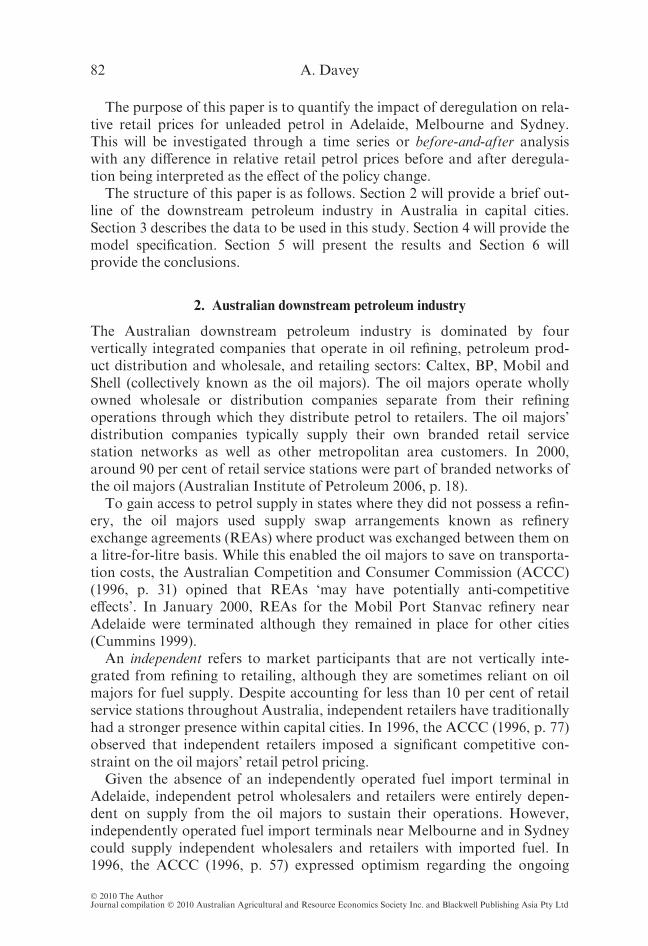
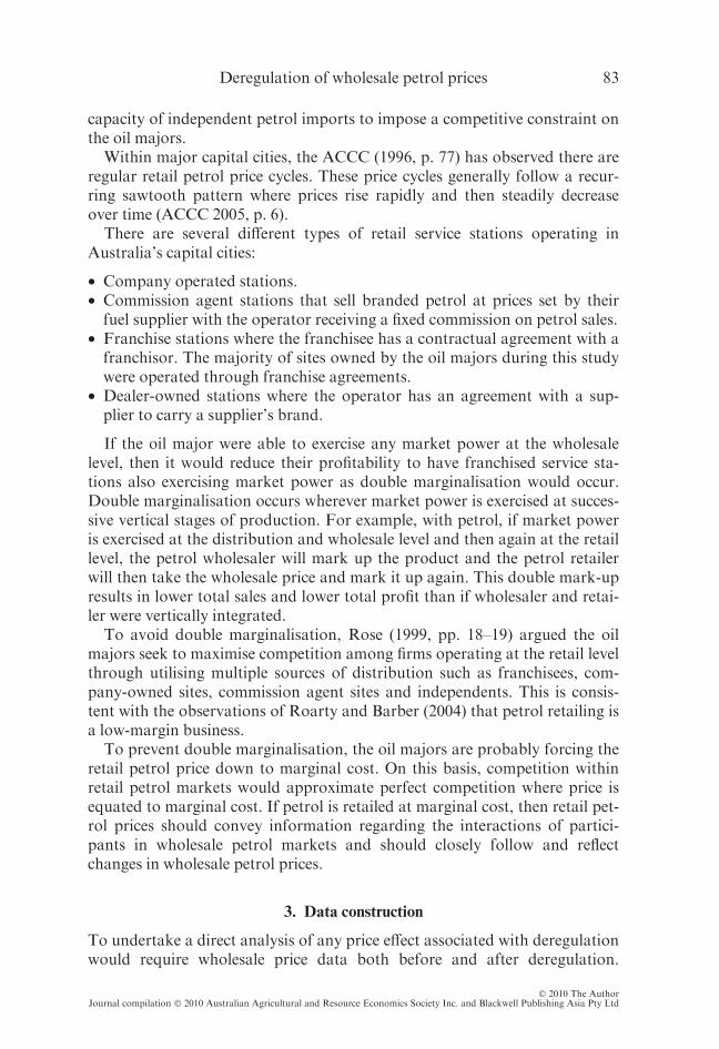
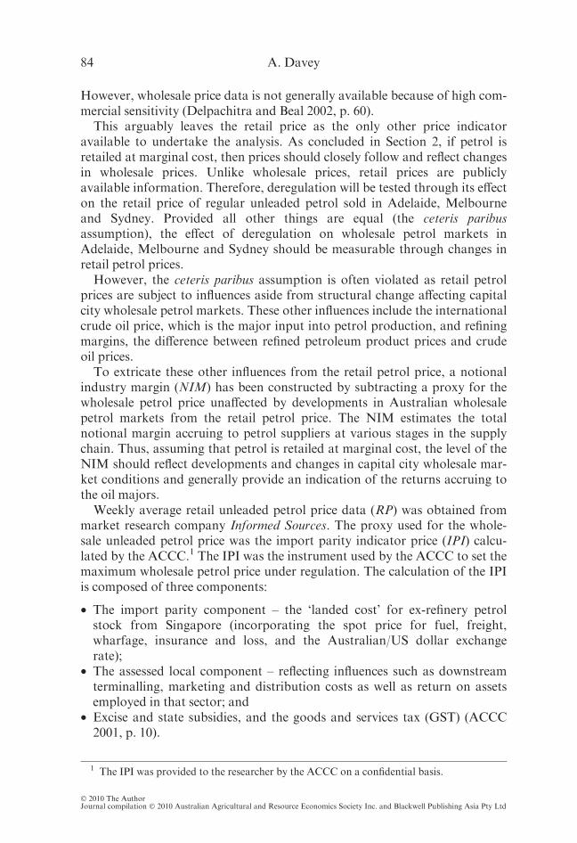
The NIM data set for Adelaide covers the period from the week beginning 30June 1997 until the week beginning 3 June 2002, representing 13 monthsbefore deregulation and 46 months after. The NIM data set for Melbournecovers the period from the week beginning 6 January 1997 until the weekbeginning 23 July 2001, representing 19 months before deregulation and36 months after. The NIM data set for Sydney covers the period from theweek beginning 6 January 1997 until the week beginning 24 June 2002, repre-senting 19 months before deregulation and 47 months after. It was decided toconclude the study for Melbourne and Sydney to control for the influence ofother events that could result in structural change. For Melbourne, this arisesfrom the regulatory imposition of terminal gate pricing in Victoria in August2001. For Sydney, this arises from the termination of REAs in July 2002.Figures 1, 2 and 3 shows that the NIM in all three cities oscillates through

time.For all three cities, the pattern of the NIM data displays no obvious

signs of seasonality although the trend appears to be heading down-wards over time with the exception of Adelaide from March 2001onwards, suggesting that deregulation generally coincided with fallingaverage levels for the NIM.

86 A. Davey


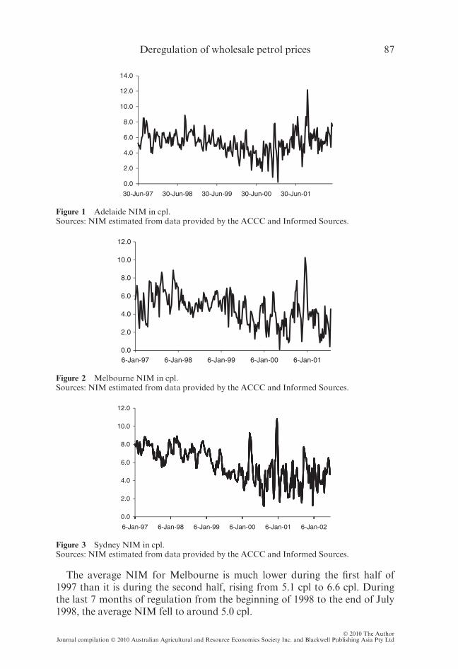
The average NIM for Melbourne is much lower during the first half of1997 than it is during the second half, rising from 5.1 cpl to 6.6 cpl. Duringthe last 7 months of regulation from the beginning of 1998 to the end of July1998, the average NIM fell to around 5.0 cpl.

0.0

2.0

4.0

6.0

8.0

10.0

12.0

6-Jan-97 6-Jan-98 6-Jan-99 6-Jan-00 6-Jan-01 6-Jan-02

Figure 3 Sydney NIM in cpl.Sources: NIM estimated from data provided by the ACCC and Informed Sources.

0.0

2.0

4.0

6.0

8.0

10.0

12.0

6-Jan-97 6-Jan-98 6-Jan-99 6-Jan-00 6-Jan-01

Figure 2 Melbourne NIM in cpl.Sources: NIM estimated from data provided by the ACCC and Informed Sources.

0.0

2.0

4.0

6.0

8.0

10.0

12.0

14.0

30-Jun-97 30-Jun-98 30-Jun-99 30-Jun-00 30-Jun-01

Figure 1 Adelaide NIM in cpl.Sources: NIM estimated from data provided by the ACCC and Informed Sources.



The average NIM for Sydney during regulation from January 1997 untilthe end of July 1998 is less volatile than for Melbourne, averaging around 7.3cpl. In Adelaide, during regulation from the beginning of July 1997 until theend of July 1998, the NIM averaged around 5.9 cpl.During the first period of deregulation from the beginning of August 1998

to the end of December 1998, the average level of the NIM rose in bothAdelaide and Melbourne, while it fell marginally in Sydney. The averageNIM for Adelaide rose to around 6.3 cpl. This rise may be related to a firethat occurred at the Port Stanvac refinery on 2 August 1998, which closeddown the refinery for 2 months. According to the Department of PrimaryIndustries and Resources South Australia (1999, p. 41), petrol stocksremained tight for 2 months following the fire. The average NIM for Mel-bourne rose to 5.5 cpl, which could be related to a reduced level of petrol dis-counting following the interruption of Victorian crude oil supplies from BassStrait in late September 1997 (Shiel 1998). In Sydney, the average NIM fellmarginally to 7.2 cpl.During the first half of 1999, the average NIM fell below the level recorded

during the entire period of regulation across all three cities. The average NIMfell to 5.5 cpl in Adelaide, 4.9 cpl in Melbourne and 6.3 cpl in Sydney.From mid-1999 onwards, the average NIM fell further across all three cit-

ies. From July 1999 until the end of July 2001, the average NIM was 3.6 cplin Melbourne. From July 1999 until the end of June 2002, the average NIMwas 4.6 cpl in Sydney. From July 1999 until the end of February 2001, theaverage NIM for Adelaide was 4.3 cpl, however, the average NIM rose to 5.9cpl coinciding with the introduction of tighter fuel standards in South Austra-lia.During 2000, there are several spikes in the NIM that stand out. There was

a spike in mid to late March in Sydney, which coincided with newspaperreports of discussions between the two locally based refiners in Caltex andShell about a possible merger of their refinery operations (Macleay 2000).There is a spike occurring in Melbourne during and in the aftermath of ablockade of Melbourne fuel terminal facilities at the end of September 2000(ACCC 2000). Finally, there is a spike in Melbourne and Sydney, and to a les-ser extent in Adelaide, occurring over the Christmas 2000 and New Year holi-day period coinciding with a period of unexpected refinery shutdowns on theAustralian eastern seaboard (PM Program 2000). There is also a spike in theNIM for Adelaide in October 2001 coinciding with a maintenance strike atthe Port Stanvac refinery that eventually forced the South Australian Gov-ernment to impose petrol rationing (Eccles 2001).

4. Model specification

To test whether there is a statistically significant difference in the average levelof the NIM before and after deregulation, a regression model was con-structed. To build a structural model for estimating the NIM would require a

88 A. Davey


reasonably complete knowledge and understanding of the NIM determina-tion process. Given the NIM is determined through the decisions and interac-tions of numerous wholesale and retail market participants, the informationrequirements arguably preclude one from attempting to build a structuralmodel.As an alternative to a structural model, an empirical model was con-

structed for the NIM using Box–Jenkins methodology, also known as auto-regressive integrated moving average (ARIMA) modelling. In ARIMAmodelling, a variable is explained by its own past, or lagged, values and sto-chastic error terms. While not providing a behavioural explanation for thetime path of the NIM, an ARIMA model should capture any underlying sys-tematic time series patterns in the data.Modelling of the NIM time series would appear to be well-suited to

ARIMA modelling. The number of observations for Melbourne is 238, forAdelaide it is 258 and for Sydney it is 286. Box et al. (1994, p. 17) maintainthat ARIMA models should only be used when at least 50 and preferably 100or more observations are available.Autoregressive integrated moving average models can also be extended

to enable the intervention analysis proposed by Box and Tiao (1975) to beutilised. Under intervention analysis, an indicator (or dummy) variable isincluded in the model, which takes only the values of 0 and 1 to denote thenon-occurrence and occurrence of the intervention as long as the timing ofthe intervention is known. Intervention analysis will be used to test for theimpact of deregulation on the NIM. The impact of regulation is generallymeasured by a dummy variable, indicating whether the observation occursduring the period of regulation or in an unregulated environment (Joskowand Rose 1989, p. 1458).One criticism sometimes made of ARIMA models is that they can be

prone to disturbances because of ‘special’ events which it is claimed caninvalidate the approach (Gregg 1980, p. 82). However, Jenkins (1979)has shown that intervention analysis can also be used to control forsuch disturbances provided satisfactory evidence exists to prove the exis-tence of an associated event. In this regard, intervention analysis willalso be used to control for the several short-term events impacting uponthe level of the NIM, namely the merger discussions between Shell andCaltex in Sydney in late March 2000, the blockade of Melbourne fuelterminals in September 2000, the reported fuel shortages along the Aus-tralian eastern seaboard during a period when there were a series ofunexpected refinery shutdowns in December 2000, and the maintenancestrike at the Port Stanvac refinery in October 2001. It will also be usedto control for any impact on the NIM arising from the termination ofREAs in regard to the Adelaide Port Stanvac refinery at the beginningof 2000 and the introduction of tighter fuel standards for South Austra-lia in March 2001.



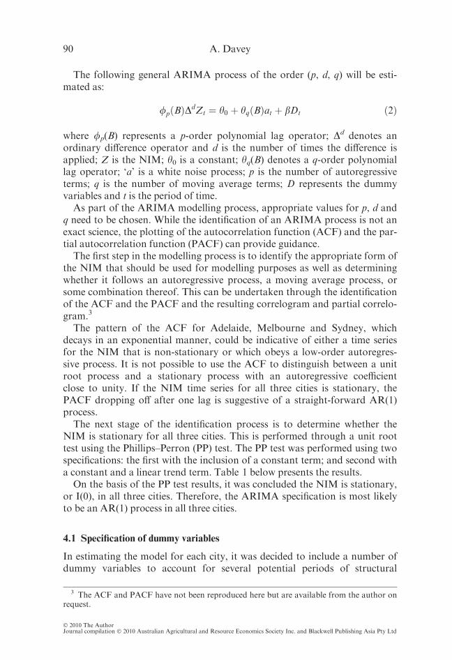
The following general ARIMA process of the order (p, d, q) will be esti-mated as:

/pðBÞDdZt ¼ h0 þ hqðBÞat þ bDt ð2Þ

where /p(B) represents a p-order polynomial lag operator; Dd denotes anordinary difference operator and d is the number of times the difference isapplied; Z is the NIM; h0 is a constant; hq(B) denotes a q-order polynomiallag operator; ‘a’ is a white noise process; p is the number of autoregressiveterms; q is the number of moving average terms; D represents the dummyvariables and t is the period of time.As part of the ARIMA modelling process, appropriate values for p, d and

q need to be chosen. While the identification of an ARIMA process is not anexact science, the plotting of the autocorrelation function (ACF) and the par-tial autocorrelation function (PACF) can provide guidance.The first step in the modelling process is to identify the appropriate form of

the NIM that should be used for modelling purposes as well as determiningwhether it follows an autoregressive process, a moving average process, orsome combination thereof. This can be undertaken through the identificationof the ACF and the PACF and the resulting correlogram and partial correlo-gram.3

The pattern of the ACF for Adelaide, Melbourne and Sydney, whichdecays in an exponential manner, could be indicative of either a time seriesfor the NIM that is non-stationary or which obeys a low-order autoregres-sive process. It is not possible to use the ACF to distinguish between a unitroot process and a stationary process with an autoregressive coefficientclose to unity. If the NIM time series for all three cities is stationary, thePACF dropping off after one lag is suggestive of a straight-forward AR(1)process.The next stage of the identification process is to determine whether the

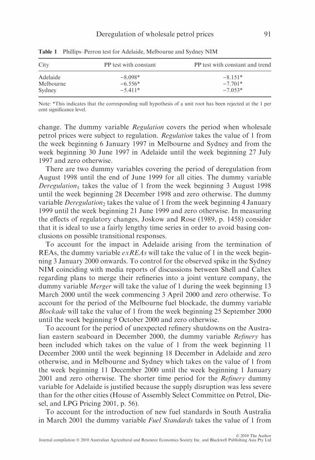
NIM is stationary for all three cities. This is performed through a unit roottest using the Phillips–Perron (PP) test. The PP test was performed using twospecifications: the first with the inclusion of a constant term; and second witha constant and a linear trend term. Table 1 below presents the results.On the basis of the PP test results, it was concluded the NIM is stationary,

or I(0), in all three cities. Therefore, the ARIMA specification is most likelyto be an AR(1) process in all three cities.

4.1 Specification of dummy variables

In estimating the model for each city, it was decided to include a number ofdummy variables to account for several potential periods of structural

3 The ACF and PACF have not been reproduced here but are available from the author onrequest.

90 A. Davey


change. The dummy variable Regulation covers the period when wholesalepetrol prices were subject to regulation. Regulation takes the value of 1 fromthe week beginning 6 January 1997 in Melbourne and Sydney and from theweek beginning 30 June 1997 in Adelaide until the week beginning 27 July1997 and zero otherwise.There are two dummy variables covering the period of deregulation from

August 1998 until the end of June 1999 for all cities. The dummy variableDeregulation1 takes the value of 1 from the week beginning 3 August 1998until the week beginning 28 December 1998 and zero otherwise. The dummyvariable Deregulation2 takes the value of 1 from the week beginning 4 January1999 until the week beginning 21 June 1999 and zero otherwise. In measuringthe effects of regulatory changes, Joskow and Rose (1989, p. 1458) considerthat it is ideal to use a fairly lengthy time series in order to avoid basing con-clusions on possible transitional responses.To account for the impact in Adelaide arising from the termination of

REAs, the dummy variable exREAs will take the value of 1 in the week begin-ning 3 January 2000 onwards. To control for the observed spike in the SydneyNIM coinciding with media reports of discussions between Shell and Caltexregarding plans to merge their refineries into a joint venture company, thedummy variableMerger will take the value of 1 during the week beginning 13March 2000 until the week commencing 3 April 2000 and zero otherwise. Toaccount for the period of the Melbourne fuel blockade, the dummy variableBlockade will take the value of 1 from the week beginning 25 September 2000until the week beginning 9 October 2000 and zero otherwise.To account for the period of unexpected refinery shutdowns on the Austra-

lian eastern seaboard in December 2000, the dummy variable Refinery hasbeen included which takes on the value of 1 from the week beginning 11December 2000 until the week beginning 18 December in Adelaide and zerootherwise, and in Melbourne and Sydney which takes on the value of 1 fromthe week beginning 11 December 2000 until the week beginning 1 January2001 and zero otherwise. The shorter time period for the Refinery dummyvariable for Adelaide is justified because the supply disruption was less severethan for the other cities (House of Assembly Select Committee on Petrol, Die-sel, and LPG Pricing 2001, p. 56).To account for the introduction of new fuel standards in South Australia

in March 2001 the dummy variable Fuel Standards takes the value of 1 from

Table 1 Phillips–Perron test for Adelaide, Melbourne and Sydney NIM

City PP test with constant PP test with constant and trend

Adelaide )8.098* )8.151*Melbourne )6.556* )7.701*Sydney )5.411* )7.053*

Note: *This indicates that the corresponding null hypothesis of a unit root has been rejected at the 1 percent significance level.



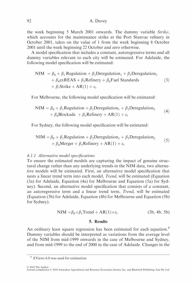
the week beginning 5 March 2001 onwards. The dummy variable Strike,which accounts for the maintenance strike at the Port Stanvac refinery inOctober 2001, takes on the value of 1 from the week beginning 8 October2001 until the week beginning 22 October and zero otherwise.A model specification that includes a constant, autoregressive terms and all

dummy variables relevant to each city will be estimated. For Adelaide, thefollowing model specification will be estimated:

NIM ¼ b0 þ b1 Regulationþ b2Deregulation1 þ b3Deregulation2

þ b4exREASþ b5Refineryþ b6Fuel Standards

þ b7StrikeþARð1Þ þ et

ð3Þ

For Melbourne, the following model specification will be estimated:

NIM ¼ b0 þ b1Regulationþ b2Deregulation1 þ b3Deregulation2

þ b4Blockade þ b5RefineryþARð1Þ þ etð4Þ

For Sydney, the following model specification will be estimated:

NIM ¼ b0 þ b1Regulationþ b2Deregulation1 þ b3Deregulation2

þ b4Mergerþ b5RefineryþARð1Þ þ etð5Þ

4.1.1 Alternative model specificationsTo ensure the estimated models are capturing the impact of genuine struc-tural change rather than any underlying trends in the NIM data, two alterna-tive models will be estimated. First, an alternative model specification thatnests a linear trend term into each model, Trend, will be estimated (Equation(3a) for Adelaide, Equation (4a) for Melbourne and Equation (5a) for Syd-ney). Second, an alternative model specification that consists of a constant,an autoregressive term and a linear trend term, Trend, will be estimated(Equation (3b) for Adelaide, Equation (4b) for Melbourne and Equation (5b)for Sydney).

NIM ¼b0þb1TrendþARð1Þþet (3b, 4b, 5b)

5. Results

An ordinary least square regression has been estimated for each equation.4

Dummy variables should be interpreted as variations from the average levelof the NIM from mid-1999 onwards in the case of Melbourne and Sydney,and from mid-1999 to the end of 2000 in the case of Adelaide. Changes in the

4 EViews 6.0 was used for estimation.

92 A. Davey


average level of the NIM can also be interpreted as changes in the relativeretail price of unleaded petrol.The estimated Ljung and Box Q-statistics for serial correlation (up to 20

lags) were not statistically significant for any equation except for Equation(3b) (5 lags) and Equation (5b) (18 lags). The Breusch–Godfrey Lagrangemultiplier test for serial correlation (Breusch–Godfrey LM test) up to 4 lagswere not statistically significant for any equation.However, the White heteroskedasticity test for all equations reveals that

the null hypothesis for the non-presence of heteroskedasticity has tobe rejected at least at the 5 per cent level suggesting that all models containheteroskedasticity. While the presence of heteroskedasticity in the regressiondoes not cause bias nor inconsistency in the parameter estimates, it doesinvalidate the standard errors, t-statistics, and F-statistics because the stan-dard errors and the confidence intervals calculated will be too narrow.According to Engle (2001, p. 158), provided the sample size is large, robust

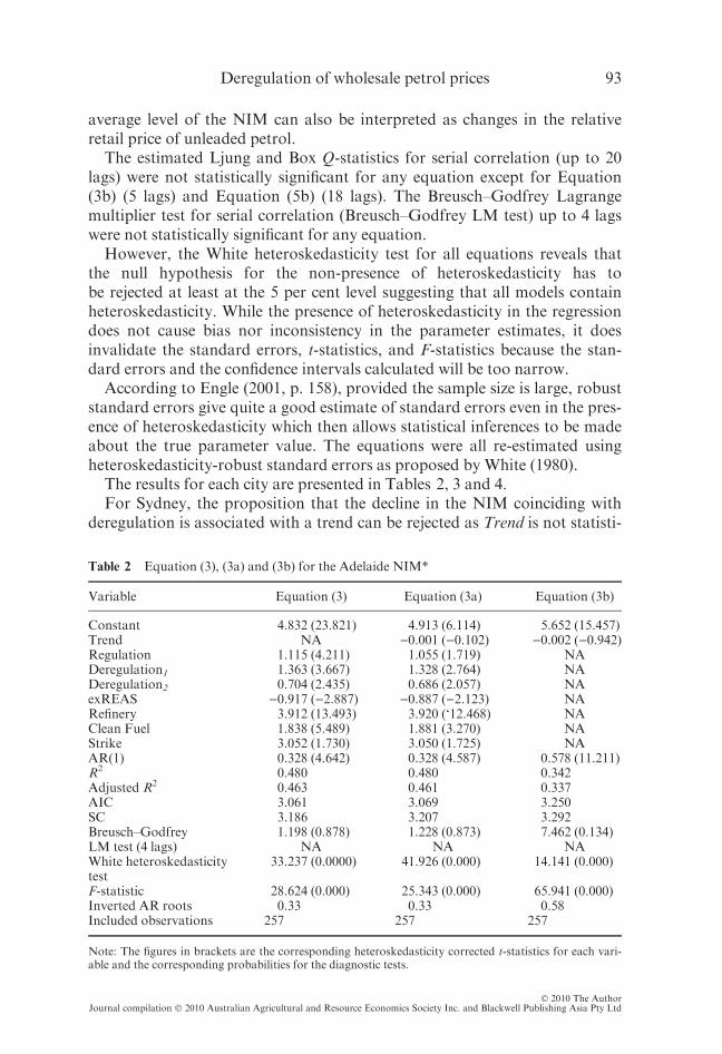
standard errors give quite a good estimate of standard errors even in the pres-ence of heteroskedasticity which then allows statistical inferences to be madeabout the true parameter value. The equations were all re-estimated usingheteroskedasticity-robust standard errors as proposed by White (1980).The results for each city are presented in Tables 2, 3 and 4.For Sydney, the proposition that the decline in the NIM coinciding with

deregulation is associated with a trend can be rejected as Trend is not statisti-

Table 2 Equation (3), (3a) and (3b) for the Adelaide NIM*

Variable Equation (3) Equation (3a) Equation (3b)

Constant 4.832 (23.821) 4.913 (6.114) 5.652 (15.457)Trend NA )0.001 ()0.102) )0.002 ()0.942)Regulation 1.115 (4.211) 1.055 (1.719) NADeregulation1 1.363 (3.667) 1.328 (2.764) NADeregulation2 0.704 (2.435) 0.686 (2.057) NAexREAS )0.917 ()2.887) )0.887 ()2.123) NARefinery 3.912 (13.493) 3.920 (‘12.468) NAClean Fuel 1.838 (5.489) 1.881 (3.270) NAStrike 3.052 (1.730) 3.050 (1.725) NAAR(1) 0.328 (4.642) 0.328 (4.587) 0.578 (11.211)R2 0.480 0.480 0.342Adjusted R2 0.463 0.461 0.337AIC 3.061 3.069 3.250SC 3.186 3.207 3.292Breusch–GodfreyLM test (4 lags)

1.198 (0.878)NA

1.228 (0.873)NA

7.462 (0.134)NA

White heteroskedasticitytest

33.237 (0.0000) 41.926 (0.000) 14.141 (0.000)

F-statistic 28.624 (0.000) 25.343 (0.000) 65.941 (0.000)Inverted AR roots 0.33 0.33 0.58Included observations 257 257 257

Note: The figures in brackets are the corresponding heteroskedasticity corrected t-statistics for each vari-able and the corresponding probabilities for the diagnostic tests.



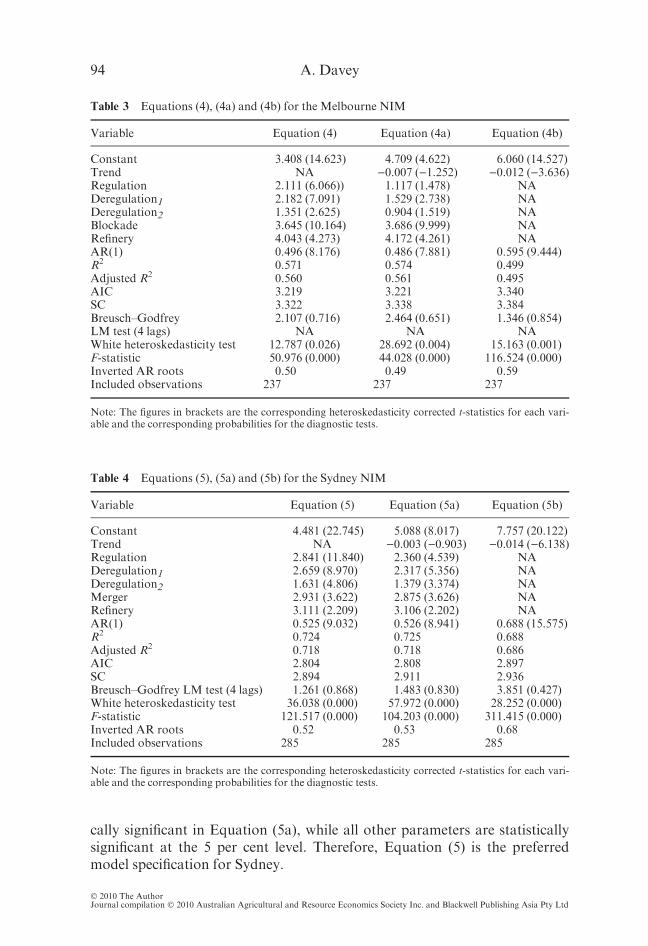
cally significant in Equation (5a), while all other parameters are statisticallysignificant at the 5 per cent level. Therefore, Equation (5) is the preferredmodel specification for Sydney.

Table 3 Equations (4), (4a) and (4b) for the Melbourne NIM


Constant 3.408 (14.623) 4.709 (4.622) 6.060 (14.527)Trend NA )0.007 ()1.252) )0.012 ()3.636)Regulation 2.111 (6.066)) 1.117 (1.478) NADeregulation1 2.182 (7.091) 1.529 (2.738) NADeregulation2 1.351 (2.625) 0.904 (1.519) NABlockade 3.645 (10.164) 3.686 (9.999) NARefinery 4.043 (4.273) 4.172 (4.261) NAAR(1) 0.496 (8.176) 0.486 (7.881) 0.595 (9.444)R2 0.571 0.574 0.499Adjusted R2 0.560 0.561 0.495AIC 3.219 3.221 3.340SC 3.322 3.338 3.384Breusch–GodfreyLM test (4 lags)

2.107 (0.716)NA

2.464 (0.651)NA

1.346 (0.854)NA

White heteroskedasticity test 12.787 (0.026) 28.692 (0.004) 15.163 (0.001)F-statistic 50.976 (0.000) 44.028 (0.000) 116.524 (0.000)Inverted AR roots 0.50 0.49 0.59Included observations 237 237 237


Table 4 Equations (5), (5a) and (5b) for the Sydney NIM


Constant 4.481 (22.745) 5.088 (8.017) 7.757 (20.122)Trend NA )0.003 ()0.903) )0.014 ()6.138)Regulation 2.841 (11.840) 2.360 (4.539) NADeregulation1 2.659 (8.970) 2.317 (5.356) NADeregulation2 1.631 (4.806) 1.379 (3.374) NAMerger 2.931 (3.622) 2.875 (3.626) NARefinery 3.111 (2.209) 3.106 (2.202) NAAR(1) 0.525 (9.032) 0.526 (8.941) 0.688 (15.575)R2 0.724 0.725 0.688Adjusted R2 0.718 0.718 0.686AIC 2.804 2.808 2.897SC 2.894 2.911 2.936Breusch–Godfrey LM test (4 lags) 1.261 (0.868) 1.483 (0.830) 3.851 (0.427)White heteroskedasticity test 36.038 (0.000) 57.972 (0.000) 28.252 (0.000)F-statistic 121.517 (0.000) 104.203 (0.000) 311.415 (0.000)Inverted AR roots 0.52 0.53 0.68Included observations 285 285 285


94 A. Davey


For Equations (3a) and (4a), neither the Trend nor the Regulation termsare statistically significant, hence resort must be made to comparing Equa-tions (3) and (4) against the alternative model specifications of Equations (3b)and (4b), respectively, to determine the preferred model specification forAdelaide and Melbourne. For Adelaide, the model specification in Equation(3b) can be rejected as the Trend term is not statistically significant, leavingEquation (3) as the preferred model specification.For Melbourne, resort must be made to choosing the preferred model spec-

ification based on the Akaike information criterion (AIC) and the Schwarzcriterion (SC) – with smaller values being preferred. Given smaller AIC andSC values for Equation (4) when compared with Equation (4b), it is con-cluded that Equation (4) is a better fit for the data than Equation (4b) and onthat basis is the preferred model specification for Melbourne.All explanatory variables for the preferred model specifications for each

city are statistically significant at less than the 1 per cent level with the excep-tion of Deregulation2 for Equation (4) and Refinery for Equation (5) whichare statistically significant at less than the 5 per cent level, and Strike forEquation (4) which is statistically significant at the 10 per cent level. Theinverted AR roots for all equations has a modulus of less than 1, suggestingthe estimated models are all stationary.The positive sign on the Regulation explanatory variable in all three cities

suggests that the regulation of wholesale petrol prices was associated with rel-atively higher retail petrol prices than was the case following deregulationafter an adjustment period. The modelling suggests that retail prices eventu-ally fell by 1.1 cpl in Adelaide, by 2.1 cpl in Melbourne and by 2.8 cpl in Syd-ney following deregulation.Sensitivity analysis was also conducted through running a series of alterna-

tive model specifications for each city. First, the autoregressive terms wereremoved from each model. Second, a basic model specification consisting of aconstant term coupled with the Regulation, Deregulation1 and Deregulation2terms both with and without the autoregressive terms was run for each city.Third, a model specification that separated out the impact of a higher averageNIM for Melbourne recorded during the second half of 1997 from the rest ofthe period of regulation was run. The main finding that retail petrol priceseventually fell in all three cities following deregulation is robust under allalternative model specifications.

6. Conclusions

The eventual fall in the average NIM following deregulation lends itself totwo possible explanations: first that the reduction was directly associated withderegulation; and second that there was some other structural change thatoccurred simultaneously across all three cities.While increased competition from independent petrol importers may

provide an alternative explanation for the fall in the average level of the NIM



following deregulation, it is unlikely to be the major factor. This is becausethere were already independently operated fuel import terminals near Mel-bourne and in Sydney able to receive imported petrol from overseas prior toJanuary 1997, so any impact from independent petrol imports was presum-ably already present from the beginning of the sample period. Furthermore,increased competition from independent petrol importers does not explainwhy the average NIM also fell in Adelaide which did not have access to anyindependent petrol imports.For Adelaide, another alternative source of structural change may be asso-

ciated with the termination of REAs from the beginning of 2000. However,even if this event was associated with a decrease in the average NIM, it hadalready fallen following deregulation prior to the beginning of 2000.The major shortcoming with trying to identify alternative sources of struc-

tural change to explain the fall in the average NIM following deregulation isthe inability to identify any alternative event that occurred simultaneouslyacross all three cities. In the absence of an alternative explanation, it is con-cluded that the fall in the average NIM was most likely associated with dereg-ulation.If deregulation was associated with relatively lower retail petrol prices, one

possible explanation is that it reduced production costs, which were eventu-ally competed away by market participants during the first half 1999 andpassed on to consumers in the form of relatively lower retail petrol prices.While the statistical significance of certain dummy variables (Merger andexREAs) are suggestive of potential competition problems in the downstreampetroleum industry, the eventual reduction in relative retail petrol prices fol-lowing deregulation suggests that capital city retail petrol markets are com-petitive to some extent, if not immediately in the short term, then at least inthe medium term in that retail petrol prices eventually adjusted to reflect pos-sible changes in the cost structure at the wholesale level. If capital city retailpetrol markets were not at least competitive in the medium term, then relativeretail petrol prices should not have fallen following deregulation, with whole-sale market participants, principally the oil majors, simply pocketing anyreduction in production costs following deregulation.5

The results of this study suggest that consumers in Adelaide, Melbourneand Sydney enjoyed relatively lower retail petrol prices following deregula-tion than would have otherwise been the case if regulation had continued andwere unambiguously better off as a result. An important policy implication isthat it suggests that not only was regulation an ineffectual policy instrumentin terms of constraining the pricing behaviour of the oil majors, but that theregulation probably imposed increased production costs that were ultimatelypaid for by consumers through relatively higher retail petrol prices. This also

5 Given that it is widely believed that demand for petrol is highly price inelastic, it would beirrational for profit maximising firms to reduce their prices unless they were engaging in pricecompetition.

96 A. Davey


suggests that future policy interventions designed to constrain prices in thedownstream petroleum industry should be very carefully considered.

References

Australian Competition and Consumer Commission (1996). Inquiry into the PetroleumProducts Declaration, vol. 1, Main Report. AGPS, Australian Competition and ConsumerCommission, Canberra.

Australian Competition and Consumer Commission (2000). Report on the Movement in FuelPrices in the September Quarter 2000. Canberra.

Australian Competition and Consumer Commission (2001). Reducing Fuel Variability: Discus-

sion Paper. Australian Competition and Consumer Commission, Canberra.Australian Competition and Consumer Commission (2005). Understanding Petrol Pricing inAustralia: Answers to Some Frequently Asked Questions. Australian Competition and Consu-mer Commission, Canberra.

Australian Institute of Petroleum (1998). Oil and Australia Statistical Review 1997. AustralianInstitute of Petroleum, Melbourne.

Australian Institute of Petroleum (2006). Submission to the Inquiry into Future Oil Supply and

Alternate Transport Fuels. Australian Institute of Petroleum, Canberra.Box, G.E.P. and Tiao, G.C. (1975). Intervention analysis with applications to economic andenvironmental problems, Journal of the American Statistical Association 70(349), 70–79.

Box, G.E.P., Jenkins, G.M. and Reinsel, G. (1994). Time Series Analysis: Forecasting and Con-trol. 3rd edn. Prentice Hall, Englewood Cliffs, NJ.

Costello, P. and Moore, J. (1998). Petroleum Marketing Reforms, media release. Joint State-ment by the Australian Government Treasurer and the Minister for Industry, Science and

Tourism, Melbourne, 20 July.Cummins, K. (1999). Mobil to halve Port Stanvac production, The Australian FinancialReview, 30 Dec (p. 3).

Delpachitra, S. and Beal, D. (2002). Petrol prices disparity: did the removal of price surveil-lance create price competition? Economic Papers 21, 56–65.

Eccles, D. (2001). Petrol rationed, The Advertiser, 17 Oct (p. 1).

Engle, R. (2001). GARCH 101: The use of ARCH/GARCH models in applied econometrics,The Journal of Economic Perspectives 15, 157–168.

Gabbitas, O. and Eldridge, D. (1998). Directions for State Tax Reform. Productivity Commis-

sion Staff Research Paper, AusInfo, Melbourne.Gregg, D.P. (1980). Reviewed work: practical experiences with modelling and forecasting timeseries by G.M. Jenkins, Journal of the Royal Statistical Society Series A (General) 143,81–82.

House of Assembly Select Committee on Petrol, Diesel, and LPG Pricing (2001). Official Han-sard Report: Monday 28 May 2001 at 4.25pm. Parliament of South Australia, Adelaide.

Jenkins, G.M. (1979). Practical Experiences with Modelling and Forecasting Time Series. Gwi-

lyn Jenkins & Partners, St Helier, Jersey.Joskow, J.L. and Rose, N.L. (1989). The effects of economic regulation, in Schmalensee, R.and Willig, R.D. (eds), Handbook of Industrial Organization. Elsevier Science Publishers

B.V., Amsterdam, pp. 1449–1506.Macleay, J. (2000). Shell, Caltex weigh refinery merger, The Australian, 15 Mar (p. 25).PM Program (2000). Petrol prices remain high over Christmas, ABC Radio, 22 Dec.

Primary Industries and Resources South Australia (1999). PIRSA Annual Report 1998–99.Primary Industries and Resources South Australia, Adelaide.

Roarty, M. and Barber, S. (2004). Petrol Pricing in Australia: Issues and Trends. Current IssuesBrief No. 10 2003-04, Information and Research Services, Parliamentary Library, Depart-

ment of Parliamentary Services, Canberra.



Rose, J. (1999). The ACCC and the market power of the oil majors – Part 1, Trade PracticesLaw Journal 7, 17–30.

Royal Commission on Petroleum (1976). Fourth Report: The Marketing and Pricing of Petro-leum Products in Australia. AGPS, Canberra.

Shiel, F. (1998). Longford slows fuel price war, The Age, 7 Oct (p. 7).White, H. (1980). A heteroskedasticity-consistent covariance matrix estimator and a direct testfor heteroskedasticity, Econometrica 48, 817–838.

98 A. Davey


Deregulation of wholesale petrol prices: what happened to capital city petrol prices

Documents

Transcript of Deregulation of wholesale petrol prices: what happened to capital city petrol prices