University of New OrleansScholarWorks@UNO

University of New Orleans Theses and Dissertations Dissertations and Theses

5-20-2011

Two Essays on Oil Futures MarketsIman AdeinatUniversity of New Orleans

Follow this and additional works at: http://scholarworks.uno.edu/td

This Dissertation is brought to you for free and open access by the Dissertations and Theses at ScholarWorks@UNO. It has been accepted for inclusionin University of New Orleans Theses and Dissertations by an authorized administrator of ScholarWorks@UNO. The author is solely responsible forensuring compliance with copyright. For more information, please contact scholarworks@uno.edu.

Recommended CitationAdeinat, Iman, "Two Essays on Oil Futures Markets" (2011). University of New Orleans Theses and Dissertations. Paper 1289.

Two Essays on Oil Futures Markets

A Dissertation

Submitted to the Graduate Faculty of the University of New Orleans in partial fulfillment of the

requirements for the degree of

Doctor of Philosophy in

Engineering and Applied Science Engineering Management

by

Iman Adeinat

B.S. University of Jordan, Jordan, 2003 M.S. University of New Orleans, USA, 2007

May, 2011

ii

Copyright 2011, Iman Adeinat

iii

Dedication

This dissertation is dedicated to my husband, Naseem who provided me with undying love and

support during these years. Without your patience and unwavering support and encouragement,

I could not have accomplished my research.

iv

Acknowledgment

I would like thank all the people who assisted and supported me during my study. First and foremost, I would like to express my gratitude to my co-chair and advisor, Prof. Peihwang Philip Wei for his careful guidance and mentoring. He exemplifies the high quality scholarship to which I aspire. Many thanks to my co-chair, Dr. Jay Hunt and my committee members, Prof. Norma Mattie, Prof. Tumulesh Solanky, and Dr. Ilhan Demiralp. They provided excellent advice and insightful commentary. Special thanks go to my dad, Prof. Mohammed Adeinat and my mom, Mrs. Asma’ Kamal who

taught me to love learning and always provided support and encouragement throughout my studies. To my sisters Duaa and Rajaa and brothers Hamza and Bashar who always gave their support across the miles. Of course, the greatest support of all came from husband and my best friend, Dr. Naseem. I am forever thankful for your greatest supports through the ups and down of emotions, and to all the sacrifices you have made for me to be able to complete this dissertation. My sons Zeid, Farris, and Majd thank you for letting your mama finish her dissertations. Finally, I would like to extend my thanks to Prof. Dinah Payne, and all the incredible people I was fortunate to work with at the Center for Hazards Assessment, Response and Technology (UNO-CHART).

v

Table of contents

List of Figures .................................................................................................................................. vi

List of Tables .................................................................................................................................. vii

Abstract .......................................................................................................................................... viii

Introduction ....................................................................................................................................... 1

Chapter 1 ........................................................................................................................................... 3

1. Introduction ............................................................................................................................ 3

2. Literature Review................................................................................................................... 6

2.1. Relationships among the Crude Oil Futures Markets ..................................................... 6

2.2. Role of Trading Cost and Trading Activity on Information Share................................. 8

3. Data ...................................................................................................................................... 12

4. Estimating the Contribution to Discovery by Markets and the Estimated Information Share ... 14

5. Method to Analyze the Role of Trading Cost and Trading Activity on Information Share 20

6. Empirical Analysis of the Role of Trading Characteristics on Information Share .............. 27

7. Robustness of the Regression Analysis ............................................................................... 35

8. Conclusion ........................................................................................................................... 37

References ................................................................................................................................... 40

Appendix A ................................................................................................................................. 44

Appendix B ................................................................................................................................. 46

Chapter 2 ......................................................................................................................................... 47

Introduction ................................................................................................................................. 47

1. Literature Review................................................................................................................. 50

2. Data ...................................................................................................................................... 56

3. Oil Backwardation ............................................................................................................... 58

4. Factors Affecting Backwardation ........................................................................................ 64

5. Conclusion ........................................................................................................................... 80

References ................................................................................................................................... 82

Appendix A ................................................................................................................................. 85

Appendix B ................................................................................................................................. 87

Vita .................................................................................................................................................. 88

vi

List of Figures

Chapter 1

Figure 1: WTI and Brent Oil Futures Trading Cost ...................................................................... 25

Figure 2: WTI and Brent Oil Futures Volatility ........................................................................... 27

Chapter 2

Figure 1:Crude Oil Spot Price and Strong Backwardation in Oil Futures .................................... 60

Figure 2: Crude Oil Spot Price and Weak Backwardation in Oil Futures .................................... 62

Figure 3: OPEC Crude Oil Production and Quota ........................................................................ 65

Figure 4: Realized Volatility for Oil Futures ................................................................................ 69

Figure 5: Crude Oil Weak Backwardation and the United States Oil Fund (USO) Trading Volume .......................................................................................................................................... 79

vii

List of Tables

Chapter 1

Table 1: Oil Futures Contract Specification ................................................................................. 13

Table 2: Summary Statistics of Prices .......................................................................................... 14

Table 3: Stationary Tests .............................................................................................................. 16

Table 4: Johansen Cointegration Test ........................................................................................... 17

Table 5: Estimating Market Interactions Using Error Correction Model ..................................... 19

Table 6: Summary Statistics of Explanatory Variables Used in Regression Analysis ................. 29

Table 7: Regression Analysis of Share of Price Discovery .......................................................... 32

Table 8: Granger Causality Wald Tests between Information Share and Trading Costs ............. 35

Chapter 2

Table 1: Summary Statistics of Futures Prices ............................................................................. 57

Table 2: Summary Statistics of Oil Backwardation ...................................................................... 59

Table 3: Regression Analysis of Weak Backwardation ................................................................ 70

Table 4: Regression Analysis of Strong Backwardation .............................................................. 74

Table 5: Role of Oil Fund on Backwardation--Regression Analysis ........................................... 76

viii

Abstract

The first chapter of this dissertation estimates the relative contributions of two major

exchanges on crude oil futures to the price discovery process-- Chicago Mercantile Exchange

(CME) and Intercontinental Exchange (ICE), using trade-by-trade data in 2008. The study also

empirically analyzes the effects of trading characteristics on the information share of these two

markets. Trading characteristics examined in the study include trading volume, trade size, and

trading costs. On average, CME is characterized by greater volume and trade size but also

slightly greater bid-ask spread. CME leads the process of price discovery and this leadership is

caused by relative trade size and volatility before the financial crisis of 2008; however post-crisis

period this leadership is caused by trading volume. Moreover, this study presents evidence that,

in times of large uncertainty in the market, the market maker charges a greater bid-ask spread for

the more informative market.

The second chapter examines the influence of expected oil price volatility, the behavior

of the Organization of Petroleum Exporting Countries (OPEC), and the US Dollar exchange rate

volatility on the backwardation of crude oil futures during the period from January 1986 to

December 2008. The results indicate that oil futures are strongly and weakly backwardated 57%

and 69% of the time, respectively. The regression analysis of weak backwardation shows that oil

volatility, OPEC overproduction (difference between quota and the actual production), and the

volatility of the US Dollar against the Japanese Yen have a positive significant effect on oil

backwardation, while OPEC production quota imposed on its members has a negative significant

effect on oil backwardation. However the volatility of US Dollar against the British Pound has

no significant effect on oil backwardation. The regression analysis of strong backwardation

produces qualitatively the same results except that volatility has no effect. In a sub-period

ix

analysis, evidence also indicates that trading volume of oil funds and backwardation are

negatively related, suggesting that oil funds increase the demand of futures relative to that of

spot.

Keywords: Oil futures, price discovery, trading characteristics, bid-ask spread, financial crisis, backwardation, OPEC, oil funds, and exchange rate.

Introduction

This dissertation consists of two essays. The first essay of my dissertation examines the

contributions of Chicago Mercantile Exchange’s (CME) and Intercontinental Exchange (ICE)’s

Futures Europe oil futures contracts to the price discovery process, using trade-by-trade data in

2008. The study also analyzes the effects of trading characteristics on the information share of

these two markets. Specifically, the study examines trading volume, trade size, and trading costs.

Since bid and ask prices are either unavailable or nonbinding in futures market, the study

estimates the daily effective bid-ask spread using Hasbrouck (2004) Gibbs estimator that is based

on the Roll’s (1984) model and Bayesian estimation. Furthermore, the essay compare the periods

before and after September 2008, when the collapse of housing finance produced a global

liquidity crunch.

The first essay find that the information share of CME and trading characteristics that

most affect information share vary substantially between pre and post crisis periods. During the

pre-crisis period, relative trade size and volatility are positively related to CME’s information

share. After the crisis, however, CME’s share drops to 87%. Moreover, trade size is no longer a

significant explanatory variable for information share; rather, trading volume is. During liquidity

crunch it is reasonable to expect that trading might contain a great degree of noise thus trade size

carries no credible information. A broader market, as represented by greater volume, would be

more informative. The essay also find evidence that during period of great uncertainty, market

makers set greater spreads to more informed market, as a protection for greater likelihood of

adverse selection problem (i.e., trading with more informed traders).

1

2

The second essay of my dissertation examines the influence of expected oil price

volatility, the behavior of the Organization of Petroleum Exporting Countries (OPEC), and the

US Dollar exchange rate volatility on oil futures backwardation during January 1986 –December

2006. Additionally, the impact of oil fund activity is examined; since oil funds are relatively

new however, the analysis involving oil fund activity utilizes a much shorter sample period

(April 2006- December 2008). Studying these factors can improve our understanding of the spot-

futures relation.

The second essay shows that oil futures generally exhibit backwardation. In specific, it

shows that oil futures are strongly and weakly backwardated 57% and 69% of the time,

respectively, during the period from January 1986 to December 2008. The study builds on

Litzenberger and Rabinowitz (1995) theory that offer an explanation for the backwardation in oil

futures based on the option pricing theory.

Furthermore, the essay finds that OPEC production quota imposed on its members has a

negative significant effect on weak and strong backwardation, while the OPEC member’s

overproduction (difference between quota and the actual production) and the uncertainty of US

Dollar exchange rate against the Japanese Yen have a positive significant effect on oil

backwardation. The results also indicate a negative association between the United States Oil

Fund (USO) volume and backwardation.

3

Chapter 1

Analyzing the Role of Trading Cost and Trading Activity on Information Share: The Case

of Crude Oil Futures Traded on CME and ICE

1. Introduction

Oil is without doubt among the most important commodities and oil futures is among the

most liquid futures contracts in the world. During 2008–9, the West Texas Intermediate (WTI)

light, sweet crude oil futures traded on the Chicago Mercantile Exchange’s (CME) Globex

electronic trading platform and the Brent crude oil futures traded on Intercontinental Exchange

(ICE)’s Futures Europe are ranked first and second, respectively, among the top 20 energy

futures and options traded in the world.1 The competition between the two markets has also

increased in recent years2. Therefore, it should be interesting to examine the interactions between

these two markets.

The main goal of this study is to estimate the contributions of CME and Brent-ICE oil

futures contracts to the price discovery process by utilizing the common factor components

(CFC) model of Gonzalo and Granger (1995), which is based on the vector error correction

model. The study also analyzes the effects of trading characteristics on the information share of

these two markets. Specifically, the study examines trading volume, trade size, and trading costs.

Since bid and ask prices are either unavailable or nonbinding in futures market, the study

1 The ranking was based on the number of contracts traded and/or cleared in terms of energy futures and options. The total numbers of traded light, sweet crude oil futures contracts on CME were around 135 million and 137 million contracts in 2008 and 2009, respectively, whereas the total numbers of traded Brent Crude Oil Futures contracts on ICE were around 68 million and 74 million contracts in 2008 and 2009, respectively.

2 For instance, on February 3, 2006, ICE started trading WTI crude oil (a U.S. energy commodity) futures on its electronic platform in London. Since then, the ICE market share of WTI futures has increased.2 As a counter-action, on September 5, 2006 the New York Mercantile Exchange (NYMEX) launched its electronically traded contracts on CME.

4

estimates the daily effective bid-ask spread using Hasbrouck (2004) Gibbs estimator that is based

on the Roll’s (1984) model and Bayesian estimation.

The only other study that analyzes the price discovery between these two markets is a

working paper by Figuerola and Gonzalo (2009). In their study they explore the price discovery

in New York Mercantile Exchange (NYMEX) and International Petroleum Exchange (IPE) that

was later acquired by ICE in 2001. They used Figuerola and Gonzalo (2010)’s3 model to assess

the contribution of each market to the price discovery process. Empirical results indicate that

NYMEX makes a larger contribution to price discovery than IPE. They also argue that these

results are likely determined by the relative liquidity in the two closely related markets.

However, their study uses relative volume as a proxy for liquidity and liquidity arguably has

many dimensions. Moreover, Johnson (2008) theoretically and empirically shows that volume is

a noisy estimator of liquidity.

Brunetti and Gilbert (2000) and Kaufmann and Ullman (2009) examine the relationship

between crude oil futures markets; however, they focus on determining the lead/lag relationship

and the causal relationships between crude oil futures markets to determine which market

dominates the others. In general, these studies indicate that NYMEX crude oil futures is the

dominant market in crude oil futures and that it is the leader in the price discovery process.

However, none examines the reasons for this dominance, although they argue that it might be

due to the fact that NYMEX crude oil futures has longer history and higher trading volume than

other markets.

3 Figuerola and Gonzalo (2010) use a general equilibrium model of the term structure of commodity markets that

takes account of endogenous convenience yields to capture the existence of backwardation (contango) structures, leading to the Gonzalo-Granger Permanent Transitory decomposition.

5

Another important objective of this study is to study whether a market’s share of price

discovery varies with the general level of liquidity. Accordingly, the sample period is chosen to

be 2008. The global financial crisis began to take hold in late 2008 and it is possible that the

resulting liquidity crunch altered the effects of trading on the relative informativeness of markets.

It should be noted that the volatility of oil market is high; for example, oil price ranged from $50

to $147 during the 2007–2008 period.

In sum, my contributions are to examine the relative contributions of crude oil futures

contracts traded on CME and ICE in the price discovery process and to assess the effects of

trading characteristics on the information share. The results of this study should provide

implications for the role of trading characteristics on the relative leadership of markets. No less

importantly, this study estimates bid-ask spread thus can examine the impact of trading costs on

information share. This study will use the Gibbs estimator as described in Hasbrouck (2004) to

estimate the effective bid ask spread in crude oil futures market. Moreover, this study analyzes

whether the importance of trading cost and trading activity vary with market conditions,

especially whether their effects change under liquidity crunch.

The remainder of the paper is organized as follows. Section two provides a more

systematic review of the literature on the relationship among crude oil futures markets and also

discusses the potential role of trading costs and trading activity on market share of information

discovery. Section three describes the data. Section four presents the estimation of market’s

contribution to price discovery. Section five presents the regression methodology to assess the

role of trading cost and trading activity on relative price leadership between the two markets, and

section six gives the results. Section seven presents robustness check for the regression analysis.

Section eight offers concluding remarks.

6

2. Literature Review

This section reviews the related studies and is divided into two subsections. Subsection

2.1 reviews the prior studies that examine the relation among crude oil futures markets. This is

followed by subsection 2.2, which discusses the potential role of trading costs and trading

activity on market share of information discovery.

2.1. Relationships among the Crude Oil Futures Markets

Previous studies investigate the causal relationship and the price discovery process

between futures and spot prices for crude oil. Silvapulle and Moosa (1999) investigate the casual

relationship between the spot and futures prices for West Texas Intermediate (WTI) light, sweet

crude oil in the U.S. Using linear causality testing, they find that futures prices lead spot prices.

On the other hand, when using a nonlinear causality test, they show that there is a bidirectional

interaction of the futures and spot prices. They argue that these results suggest a simultaneous

reaction to new information.

Kaufmann and Ullman (2009) also examine the causal relationships among crude oil

prices from markets in North America, Europe, Africa, and the Middle East on both the spot

market and futures markets. They argue that the existence of causal relationships is consistent

with the implication of imperfect markets, in which changes may first appear in the price of one

or more markets, as new information about the supply/demand balance becomes available, and

these changes may subsequently spread to all markets. They analyze 90 bivariate casual

relationships for 10 spot and futures markets.4 Of the 90 estimated error correction models, they

find 21 statistically significant relationships. The map of these 21 relationships shows two 4 These markets include: WTI far month futures of U.S., WTI near month futures of U.S., WTI spot of U.S., Brent

far month futures of London, Brent near month futures of London, Brent spot of London, Dubai near month futures of United Arab Emirates (UAE), Dubai spot of UAE, Bonny spot of Nigeria, and Maya spot of Mexico.

7

gateways for innovations, by which they mean a crude oil market that ―Granger causes‖ the price

of other crude oil markets but is not ―Granger caused‖ by the price of other crude oil market.

One innovation gateway is originated in Dubai spot prices and the other innovation gateway is

originated from the WTI-far month futures contract traded in NYMEX.

Brunetti and Gilbert (2000) model the volatility of the two closely related markets,

NYMEX and IPE (now ICE) crude oil futures markets. Their results imply that IPE volatility

reacts to shocks to NYMEX volatility much more strongly than NYMEX does to the IPE; thus,

the dominant volatility linkage is from NYMEX to the IPE. Moosa (2002) confirms the

leadership of the petroleum futures market in the price discovery process. He uses the daily spot

and futures prices of WTI crude oil between January 2, 1985 and July 11, 1996 in a system of

two seemingly unrelated time series equations and allows the coefficients to be time-varying; his

empirical results indicate that 60% of the price discovery function is performed in the futures

markets. Also, an earlier study by Schwarz and Szakmary (1994) finds evidence that the futures

prices for crude oil traded on the NYMEX leads the crude oil spot prices. Specifically, they find

that crude oil futures lead the price discovery process for the sample period of January 1, 1984,

to May 15, 1991. Schwarz and Szakmary (1994) findings suggest that the futures market in

crude oil is the dominant market for price leadership. Moreover, they argue that these findings

are consistent with the tremendous growth and success of the energy futures contracts traded at

the NYMEX.

Rappaport (2000) argues that energy futures facilitate price discovery, in which exchange

provides a centralized, open, liquid forum for buyers and sellers to conduct business, and by

which the prices of all transactions conducted therein are publicly disseminated. Moreover

energy futures contracts improve liquidity and price transparency since they permit hedging, by

8

giving market participants the ability to shift their exposure to other participants who are more

willing to bear that risk. Rappaport (2000) also points out the increasingly important role of the

NYMEX energy futures contracts and argues that it becomes the world’s most actively traded

contract for a physical commodity and a worldwide pricing benchmark.

2.2. Role of Trading Cost and Trading Activity on Information Share

Fleming, Ostdiek, and Whaley (1996) argue that in perfectly frictionless and rational

markets, new information should be reflected in the prices of all markets simultaneously.

However, the magnitude of trading costs differ among these markets, and thus price discovery

will tend to occur in the lowest-cost market, as it generates the highest net profit. Their trading

cost hypothesis suggests that markets with the lowest trading cost will provide the leadership in

price discovery; this hypothesis differs from the leverage hypothesis that states that price

discovery occurs in derivative markets because futures and options require smaller capital

outlays. Fleming et al. (1996) assess the magnitude of trading costs in the stock, stock option,

index option, and index futures markets by analyzing the bid ask spread and trading volume data

during March 1991. According to their trading cost hypothesis, markets with the lowest trading

costs should lead the price discovery. Empirically, they find S&P 100 index options lead the

underlying S&P 100 index and S&P 500 index futures leads the S&P 500 stock index. Since

trading S&P 500 futures costs around 3% of the cost of trading an equivalent stock portfolio, the

results are largely consistent with the trading cost hypothesis. They also find that S&P 500

futures prices lead slightly the prices of both S&P 100 index put and call options. This result is

consistent with the fact that the direct trading costs in the S&P 100 option market are higher than

9

those in the S&P 500 futures market. Overall, the results provide support for the trading cost

hypothesis.

Other studies, most of which look at equity-related markets, find empirical evidence that

supports the trading cost hypothesis. For example, Eun and Sabherwal (2003) examine price

discovery for a sample of Canadian stocks listed on both Toronto Stock Exchange (TSE) and

U.S. exchange. They find a negative relationship between the TSE share of price discovery and

the ratio of quoted spreads on the U.S. exchange and the TSE. A lower ratio of spreads implies a

greater competitive threat faced by the TSE market makers from the U.S. market makers; hence

their findings support the trading cost hypothesis. Other studies that examine stock index futures

and their respective cash market (see Kim, Szakmary, and Schwarz, 1999) and that oversee stock

index futures and index options (e.g., Hsieh, Lee, & Yuan, 2008; De Jong & Donders, 1998) also

find support for the trading cost hypothesis.

Easley and O'Hara (1987) market structure research has given greater attention to the

effect of asymmetric information on market prices. They propose a generalized model in which

the market maker does not know whether any of the traders are informed or whether all of them

are uninformed. They show that trade size introduce an adverse selection problem into security

trading. It is because informed traders prefer to trade large amounts at any given price provided

that they wish to trade. As a result, the larger the trade size, the more likely that the market

makers trade with informed traders. The optimal pricing strategies for the market makers is then

to quote bid and ask prices depending on trade size, specifically quoting larger spread for larger

trades. Therefore, trade size affects security prices by changing traders’ perception of the true

value of the underlying asset.

10

Some studies suggest a link between volatility and price discovery. For example,

Martens (1998) studies the German bund futures traded at LIFFE (floor trading system) and the

Deutsch Terminborse (DTB) (electronic trading system). He finds that in periods of high

volatility the German bund futures traded on LIFFE make a larger contribution to price discovery

than the electronically traded German bund futures contracts traded on the DTB; however, in

periods of low volatility the DTB German bund futures is more efficient although it has smaller

volume share. Martens (1998) argues that his results are consistent with the fact that open outcry

has an advantage over electronic trading systems in volatile periods because floor traders can

observe the actions of other traders; which, in turn, helps the floor traders to react faster.

A recent study by Schlusche (2009) also confirms Martens (1998) findings, using the

German blue chip index DAX: Exchange traded funds (ETFs) and index futures. He uses the

VECM model and the common factor component weights of Gonzalo and Granger (1995), to

assess the price leadership. Schlusche (2009) finds evidence that futures markets lead the process

of price discovery, and that this leadership is caused by volatility and not liquidity (measured as

relative liquidity). He also shows that, from low to high volatility periods, the share of price

leadership of the DAX index futures contracts decreases, whereas trading volume increases

relative to the DAX-ETF market. He argues that, in periods of high volatility, trading volume,

number of contracts traded, and the relative volume in the DAX index futures contracts increase,

causing a shift in informational efficiency in favor of the ETF. Thus, his findings support

Martens (1998)’s results that volatility is a factor in the price discovery process. Franke and

Hess (2000) also provide empirical evidence that support volatility is a factor in the price

discovery process while studying the Bund futures traded on LIFFE and DTB from 1991 to

1995.

11

On the other hand, Ates and Wang (2005) fail to find support for volatility as a

determinant of price discovery. In their study, they examine the price discovery between regular

index futures (floor trading system) and E-mini index futures (electronic trading system) in the

S&P 500 and NASDAQ 100 index futures using both the information shares of Hasbrouck

(1995) and the common factor weights of Gonzalo and Granger (1995)’s techniques. They find

that since 1998, the contribution made by E-mini index futures has been greater than the regular

index futures. Furthermore, they investigate the determinants of the rate of price discovery

process using regression analysis and find evidence that relative liquidity (measured by market

shares and the ratio of bid-ask spreads) and operational efficiency (measured by market activity)

jointly determine the rate of price discovery process. On the other hand, they find that volatility

(measured by daily high-low volatility estimate and daily realized volatility) is statistically

insignificant.

Other studies also suggest trading systems matter in terms of price discovery. Hasbrouck

(2003) and Ates and Wang (2005), among others, examine price discovery under alternative

trading systems in the U.S. exchanges. They find that the electronic trading system leads the

price discovery process compared with other trading systems, namely open-outcry. They argue

these results are consistent with the advantages offered by the electronic trading system;

specifically, it offers faster speed and accuracy of processing transactions, lower trading cost,

and more liquidity. In addition, Tse, Bandyopadhyay, and Shen (2006) argue that electronic

trading offers an advantage of anonymous trading.

12

3. Data

This study uses intraday data to analyze the effects of trading characteristics on the

information share of price discovery between the West Texas Intermediate (WTI) light, sweet

crude oil futures (electronic) traded on CME (WTI-CME hereafter) and the Brent crude oil

futures (electronic) traded on ICE Futures of London (Brent-ICE hereafter). The study covers

the year 2008, from January 2 to December 31. The year 2008 was a very volatile year, which is

suitable for this study since it investigates information flow between the U.S. and UK markets

and greater volatility might reflect greater information flow. The data are purchased from Tick

Data Inc.

The continuous series of futures prices is generated by using the midpoint of the bid and

ask quotes at five-minute intervals, which results in 75,952 observations spanning from January

2008 to December 2008. To assess market contribution however, the methodology requires both

markets to be open at the same time, hence the total number of 5-minute observations (intervals)

declines to 47,568 for the 257 trading days in my sample. That is, the analysis excludes 28,168

(37%) observations when the two markets are not simultaneously open. Table 1 shows the

trading times as well as contract specifications for the two markets. The CME trades the light

sweet crude oil futures contracts in units of 1,000 barrels, with a minimum price fluctuation of

$0.01 per barrel, with a physical settlement. The electronic trading is conducted on the CME

Globex trading platform and runs from 5:00 p.m. to 4:15 p.m. CST, Sunday through Friday, with

a 45-minute break each day beginning at 4:15 p.m. The ICE Futures trades Brent crude oil

futures contracts of 1,000 barrels with a minimum price fluctuation of $0.01 per barrel with cash

settlement. In April 2005, ICE transferred Brent crude oil futures floor trading to an electronic

13

trading system. The electronic trading starts at 7:00 p.m. CST and closes at 5:00 p.m. CST the

following day.

Table 1: Oil Futures Contract Specification

The table reports the contract specification of the West Texas Intermediate (WTI) light, sweet crude oil futures of U.S. and Brent crude oil futures of UK.

West Texas Intermediate (WTI)

light, sweet crude oil futures

Brent Crude Futures

Trading hours Sunday - Friday 6:00 p.m. - 5:15

p.m.(Eastern time) with a 45-minute break each day beginning at 5:15 p.m. (Eastern time)

Open 01:00 London local time (23.00 on Sundays) Close 23:00 London local time.

Contract unit 1,000 barrels 1,000 barrels Price quotation U.S. Dollars and Cents per barrel U.S. dollars and cents per barrel Trading

Period/Strip

Crude oil futures are listed nine years forward using the following listing schedule: consecutive months are listed for the current year and the next five years; in addition, the June and December contract months are listed beyond the sixth year. Additional months will be added on an annual basis after the December contract expires, so that an additional June and December contract would be added nine years forward, and the consecutive months in the sixth calendar year will be filled in.

A maximum of 72 consecutive months will be listed. In addition, 6 contract months comprising of June and December contracts will be listed for an additional three calendar years. Twelve additional contract months will be added each year on the expiry of the prompt December contract month.

Settlement Type Physical The ICE Brent Crude futures

contract is a deliverable contract based on EFP delivery with an option to cash settle, i.e the ICE Brent Index price for the day following the last trading day of the futures contract.

Venue CME Globex, CME ClearPort

ICE Clear Europe

14

Table 2 provides summary statistics of the logarithm futures price for the two markets.

The price series in both markets show positive kurtosis, indicating a leptokurtic, or fat tail. Also,

the price series in both markets have non-normal distribution, according to the Jarque-Bera (J-B)

test. The large ² values of J-B test statistics for return series are most likely due to the large

values of the kurtosis coefficients estimated.

Table 2: Summary Statistics of Prices

The table summarizes the 5-min logarithm futures prices of West Texas Intermediate (WTI) light, sweet crude oil futures traded on CME (WTI-CME) and the Brent crude oil futures traded on ICE Futures of London (Brent-ICE). The notation ―a‖ refers to significance at 1% level.

WTI-CME Brent-ICE

Mean 4.548 4.536

Variance 0.116 0.117

Skewness -1.125a -1.031a

Kurtosis 0.323a 0.081a

Jarque-Bera 10275.687a 8484.861a

4. Estimating the Contribution to Discovery by Markets and the Estimated Information Share

Hasbrouck (1995)’s5 information shares and Gonzalo and Granger (1995)’s

6 common

factor component model are the two methods most commonly utilized to assess the contribution

of one market to the price discovery to the other market based on the vector error correction

model (VECM). However, Baillie, Booth, Tse, and Zabotina (2002) and De Jong (2002) both

5 See Shastri, Thirumalai and Zutter (2008) and Fung and Tse (2008), among others. 6 See Eun and Sabherwal (2003), Harris, McInish, and Wood (2002), and Harris, McInish, Shoesmith, and Wood (1995), among others.

15

show that the two models are closely related and complement each other. In fact, both models

provide different views of the price discovery process between markets. More specifically,

Gonzalo and Granger’s model focuses on the components of the common factor and the error

correction process; whereas Hasbrouck’s model takes into account the variability of the

innovations in each market’s price. In addition, Harris, McInish, and Wood (2002) argue that the

common factor components recover the true information share in a wide range of financial

market microstructure models.7

This study employs the common factor components of Gonzalo and Granger (1995),

which decomposes the common factor into a linear combination of the prices; the coefficients of

the model indicate the amount of contribution of each market to the price discovery process.

To justify the use of VECM, the two futures price series should be tested for unit root to

establish that price series are integrated of order one. I use the Augmented Dickey-Fuller (ADF)

test to check for the presence of a unit root in each price series. ADF unit root tests are

conducted by estimating the following three regression equations for each price series (Pt) as

follows:

t

Q

i

itttt ePPP

1

1 , (1)

t

Q

i

itttt ePPcP

1

10 , (2)

t

Q

i

itttt ePPtccP

1

110 , (3)

where Q is the number of the lags in the model, which is determined by the Schwarz Bayesian

criterion (Schwarz, 1978). The three regression equations are similar to each other; the only 7 The market microstructure literature examines the relationship between trading and information flow and how the

structures of markets might affect that relationship.

16

difference is that equation (2) incorporates the presence of a drift, while equation (3)

incorporates the presence of linear time trend. The null hypothesis for ADF unit root test is that

=0 in all three cases. If the null hypothesis is rejected, then Pt contains a unit root.

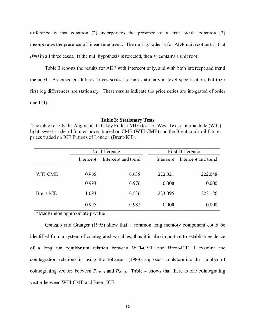
Table 3 reports the results for ADF with intercept only, and with both intercept and trend

included. As expected, futures prices series are non-stationary at level specification, but their

first log differences are stationary. These results indicate the price series are integrated of order

one I (1).

Table 3: Stationary Tests

The table reports the Augmented Dickey Fuller (ADF) test for West Texas Intermediate (WTI) light, sweet crude oil futures prices traded on CME (WTI-CME) and the Brent crude oil futures prices traded on ICE Futures of London (Brent-ICE).

No difference First Difference Intercept Intercept and trend Intercept Intercept and trend

WTI-CME 0.905 -0.638 -222.021 -222.048

0.993 0.976 0.000 0.000

Brent-ICE 1.093 -0.536 -223.095 -223.126

0.995 0.982 0.000 0.000

*MacKinnon approximate p-value

Gonzalo and Granger (1995) show that a common long memory component could be

identified from a system of cointegrated variables, thus it is also important to establish evidence

of a long run equilibrium relation between WTI-CME and Brent-ICE. I examine the

cointegration relationship using the Johansen (1988) approach to determine the number of

cointegrating vectors between PCME,t and PICE,t. Table 4 shows that there is one cointegrating

vector between WTI-CME and Brent-ICE.

17

Table 4: Johansen Cointegration Test

The table reports the Johansen cointegration test for West Texas Intermediate (WTI) light, sweet crude oil futures prices traded on CME (WTI-CME) and the Brent crude oil futures prices traded on ICE Futures London (Brent-ICE). The notation ―a‖ refers to significance at 1% level.

Eigen value Trace Maximum Eigen

WTI-CME Brent -ICE

None 0.008 371.058a 369.264a

At most 1 3.77E-05 1.794 369.264

If there are cointegration relations among both markets’ futures prices, the Granger

representation theorem (Engle and Granger, 1987) implies that there exists a specification of the

vector error correction model (VECM) as follows:

Q

q

CME

t

Q

q

CME

qtq

ICE

qtq

CME

t

CMEICE

t

CMECME

o

CME

t

Q

q

ICE

t

Q

q

CME

qtq

ICE

qtq

CME

t

CMEICE

t

ICEICE

o

ICE

t

PPPPP

PPPPP

1 1

111

1 1

111

)(

)(

, (4)

where CME

tP and ICE

tP are the first log difference of futures prices for WTI-CME and Brent-

ICE, respectively. PCME and PICE are the log prices of WTI-CME and Brent-ICE respectively.

CME is the cointegration vector between the two markets such that CME

t

CMEICE

t

ICE PP 11 is

cointegrated of order one, denoted by I(1). Q is the number of the lags in the model based on the

multivariate Schwarz Bayesian criterion (Schwarz, 1978). The coefficients ICE

0 and CME

0 are

constants. The coefficients of the error correction terms ICE

1 and CME

1 (adjustment coefficients)

indicate the responsiveness of the price series to any deviation from the equilibrium relationship

18

(i.e., the deviation of price difference between the two markets from zero). CME and ICE are the

unautocorrelated residuals.

Following Gonzalo and Granger (1995)’s common factor component model, the relative

contribution of one market to the price discovery process, or information share or the share of

price discovery, is denoted as The WTI-CME share of price discovery CME can be calculated

as follows:

CMEICE

ICE

CME

11

1

, (5)

where CMEICE

11 represents the total adjustment to restore the equilibrium relation of prices.

A higher value of CME reflects a larger contribution from WTI-CME to the price discovery.

Similarly, the higher the value of (1-CME), the larger the contribution of Brent-ICE crude oil

futures.

With the futures price series of the WTI-CME and Brent-ICE being integrated of order

one I(1) and cointegrated, model (4) is estimated with one lag as suggested by the Schwarz

Bayesian criterion. Table 5 shows the results of the estimation. The coefficients of the error

correction term (α) show that the WTI-CME generates more price discovery than Brent-ICE as

indicated by the positive sign of the error correction term ( CME

1 = 0.001). On the other hand,

Brent-ICE market responds to the WTI-CME market, as indicated by the negative sign of the

error correction term ( ICE

1 = -0.009). Table 5 also shows a strong impact of WTI-CME on the

Brent-ICE contract, and there is little feedback from the Brent-ICE market to the WTI-CME

market since the coefficient of the ICE

tP 1 is not significant.

19

Table 5: Estimating Market Interactions Using Error Correction Model

The table presents the results for the estimation of the vector error correction model as described in equation (4). Share of price discovery () is the relative contribution of one market to the price discovery process using the common factor component of Gonzalo and Granger (1995). The t-values are given in parentheses. The notations ―a‖, ―b‖ and ―c‖ refer to significance at 1, 5 and 10% level, respectively.

Full sample

Before financial crisis (Jan - Aug 2008)

After financial crisis (Sep - Dec 2008)

WTI-CME

Brent-ICE

WTI-CME

Brent-ICE

WTI-CME

Brent-ICE

Constant (0) -2.0E-05c -3.1E-06 6.2E-06 1.9E-07 -7.0E-05b -1.1E-05

(-1.72) (-0.27) (0.67) (0.02) (-2.44) (-0.37)

Error Correction Term (1)

0.001a -0.009a 0.000+ -0.010a 0.002c -0.010a

(2.84) (-18.68) (0.54) (-17.92) (1.75) (-11.78)

PtICE (1) -0.000+ -0.019a -0.001 -0.016a -0.000+ -0.021a

(-0.04) (-4.19) (-0.09) (-2.77) (-0.04) (-2.65)

PtCME (1) -0.014a -0.016a -0.012b -0.016a -0.015c -0.018b

(-2.92) (-3.47) (-2.03) (-2.89) (-1.86) (-2.32)

R2 (%) 0.04 0.80 0.02 1.07 0.07 0.93

Chi2 20.4a 375.2a 5.1 330.6a 11.8b 153.9a

Log likelihood 428496.8 305828.3 137740.6

Share of price discovery ()

86.57% 13.43% 96.97% 3.03% 86.92% 13.08%

I further test the contribution to the price discovery from the two markets during the low

and high volatility periods; thus, I split the sample into two subperiods. The first period

represents the months before the financial crisis (January–August 2008) and the second period

represents the months after the financial crisis (September–December 2008).

20

Based on the VECM results, I estimate the share of price discovery for the two markets

using equation (5). It can be seen in table 5 that during 2008 the contribution of the WTI-CME

market averages 87%, while the Brent-ICE contribution to the price discovery process averages

only 13%. The contribution of the WTI-CME market is around 97% in the months before the

financial crisis, and then it drops to around 87% in the months following the financial crisis.

This drop in CME’s contribution might be explained by the fact that the 2008 financial crisis was

global, thus the degree of market interaction increases after the crash. In sum, it is clear that the

WTI-CME market leads the price discovery process but the variations in contribution over time

can be substantial.

5. Method to Analyze the Role of Trading Cost and Trading Activity on Information

Share

One of the main purposes of the paper is to examine the role of trading cost and trading

activity on the information share of the two markets. To this end, the study performs a time

series regression of the daily WTI-CME price discovery share8 (θt

CME) on the relative volume,

relative trading cost, relative trade size, and aggregate volatility. More specifically, the

regression model is estimated as follows:

tt

CME

t

CME

t

CME

t

CME

t VolatilityTradeSizeTradeCostVolume 43210 , (6)

where VolumetCME is the relative volume, computed as the daily volume of the WTI-CME to the

total volume of WTI-CME and Brent-ICE futures on day t (volumetCME

/ volumetCME

8 It should be noted that I use a substantial number of 5-minute observations to estimate the price discovery share

(θ) for each day.

21

+volumetICE). TradeCostt

CME is the relative estimate of the effective bid ask spread of WTI-CME

to Brent-ICE using the Gibbs estimator described in Hasbrouck (2004)

(TradeCosttCME

/TradeCosttICE). TadeSizet

CME is the relative trade size defined as the average

trade size of WTI-CME to the average trade size of Brent-ICE futures on day t. Volatilityt is the

sum of the two markets’ volatility (voltCME

+voltICE) on day t.

Liquidity is not easily measured by one number alone. Most of the extant studies use the

relative volume as a proxy for liquidity, and therefore volume is also included in this study.

Hasbrouck (1995) finds a positive correlation between New York Stock Exchange (NYSE)

information share and its trading volume. Moreover, Theissen (2002) finds positive correlation

between the common factor weights of the electronic stock market of Germany and its trading

volume. Hence, it is expected that the coefficient of the relative trading volume (VolumetCME) to

be positive.

Although trading volume is one of the most commonly used measures for market

liquidity, trading volume may not adequately captures liquidity as some studies such as Johnson

(2008) suggest that volume is a noisy indicator of liquidity. Consequently, trade size and trading

cost are also analyzed here. Easley and O’Hara (1987 JFE) find evidence that larger trades are

more likely to come from informed traders. Hence, it is expected that the exchange with larger

average trade size would be more informative. As pointed out earlier, some studies suggest that

the market with lower trading cost likely attracts more traders thus more informative trading.

Trading costs include commissions and bid-ask spread (the difference between purchase and

selling prices at a given point in time). Commissions vary slightly among brokers though they

are small in general. On the other hand, literature generally views bid-ask spread as a

compensation for market making and can reflect the degree of information asymmetry. In the

22

sense, it is an important dimension of liquidity. However, bid-ask data is unavailable and bid-ask

quotes are often non-binding on floor trading. Therefore, bid-ask spread needs to be estimated.

This study uses Hasbrouck (2004) Gibbs estimator; Hasbrouck claims that it is fairly efficient

and reliable estimate of spread. A brief comparison of alternative spread estimates is given

below.

The earlier estimator for the bid-ask spread in the futures market was proposed by Roll

(1984). He argues that, if markets are informationally efficient, then the covariance between

futures price changes is directly related to the bid-ask spread. Roll’s measure (RM) can be

written as,

),cov(2 1 tt ppRM . (7)

However, when the covariance between adjacent price changes is positive, Roll’s

measure cannot be used.

Another method used to estimate the bid-ask spread in the futures market is the

Thompson and Waller (1988) estimator. They argue that the average absolute price changes are

a direct measure of the average execution cost of trading in a contract. Their estimator (TW) can

be written as

T

t tpT

TW1

1, (8)

where pt is the series of nonzero price changes. This estimator was applied by, for example,

Thompson and Waller (1988), Tse and Zabotina (2004), and Tse and Bandyopadhyay (2006), to

23

study the liquidity costs in some futures contracts. However, Thompson-Waller estimate gives

an upward bias of the spread because it fails to recognize the variance of true price changes

contained in the absolute value of price changes.

Hasbrouck Gibbs estimator (Hasbrouck, 2004) is based on the Roll’s model and Bayesian

estimation using the Gibbs estimator (Markov Monte Carlo estimator) to infer the effective bid-

ask spread from the times series of transaction prices. This estimator was applied by many

studies such as Rangel (2005), Bekaert, Harvey, and Lunblad (2007), Brick, Palmon, and Patro

(2007), and McLean (2010).

In Roll’s model, markets are assumed to be efficient; thus, let Mt represent the efficient

price that follows a random walk. The efficient price in the absence of transaction costs reflects

all available public information. In the futures market, dealers post bid (bt) and ask (a

t) prices.

Buyers buy at the ask price at and sellers receive the bid price bt

cma

cmb

tt

tt

, (9)

in which mt is the log efficient price and c is the transaction cost. As a result the prices p

t that

everyone observes when trading takes place are modeled as

ttt

tttt

cqmp

Nuumm

),0(~ 2

1 , (10)

in which qt represents the direction of the incoming order and is given by the Bernoulli random

variable qt{-1, +1}, where -1 indicates an order to sell, and +1 represents an offer to buy. Thus

depending on qt, the (log) transaction cost price is either at the bid or the ask.

24

1

1

tt

tt

tqifa

qifbp (11)

Thus, the spread model (10) implies

ttttttt uqccqmcqmp )( 11 . (12)

Conventionally, equation (12) is estimated using the moment estimates. Solving for var

(pt) and cov(pt,pt-1) yields the following estimators:

22 2)var( cp ut . (13)

2

1),cov( cpp tt . (14)

In the Bayesian approach, the parameters are viewed as random variables. The Gibbs

estimator facilitates the Bayesian approach by using an algorithm to generate a sequence of

samples from the conditional probability distributions of random variables. This algorithm is

motivated because it is applicable when the joint distribution is not known but the conditional

distribution of each variable is known. As a Markov chain Monte Carlo method, the Gibbs

sampler generates sample values from the distribution of each variable in turn, conditional on the

current values of the other variables. In equation (12), the unknown parameters are the

transaction cost c, 2

u , and the joint distribution F(q,c,2u|p).

25

The Gibbs sampler is used to obtain sample values (q(i),c

(i),2

u(i)

|p) F(q,c,2u|p) based

on the conditional distribution of pt. This method is implemented using n random draws, which

converge in distribution to the joint distribution after a sufficiently large number of iterations.

The liquidity cost is then computed as the first moment of the marginal distribution f(c|p). The

implementation of the algorithm starts with the initial values (c(0),2

u(0)

, q(0)

) then the next draws

are:

1. Draw c(1) from f(c|u(0)

, q(0)

, p)

2. Draw u(1) from f(u |c

(1), q

(0), p)

3. Draw q(1) from f(q| c(1)

, u(1)

, p)

Figure 1 shows the estimated daily average trading cost of the WTI-CME futures and the

Brent-ICE futures for the year 2008. As seen in the figure, the trading cost in both markets move

closely together. However, the trading cost after September 79 for both markets increased

substantially and the variation in trading costs is large; also the pikes are consistent with main

events during the crisis; for example the highest bid-ask for the U.S. contract was on December

17 when the U.S. Federal Reserve reduced its interest rate to 0.25%.

According to the trading cost hypothesis, informed traders react more quickly to new

information in markets with the lowest trading cost; thus, it is expected that the coefficient of the

relative trading cost (TradeCosttCME ) is inversely related to the WTI-CME price discovery share.

Figure 1: WTI and Brent Oil Futures Trading Cost

West Texas Intermediate (WTI) light, sweet crude oil futures of U.S. and Brent crude oil futures of UK trading cost measured using Hasbrouck (2004).

9 On September 7, 2008, Fannie Mae and Freddie Mac, which are agencies that provide liquidity to the mortgage

market, were rescued by the government.

26

The daily volatility is measured as the sums the squares of intraday returns (Andersen et

al., 2001a, b). Figure 2 shows the daily volatility for the WTI-CME and Brent-ICE in the year

2008. As seen in the figure, the volatility in both markets moved closely together; after

September 7, volatility for both markets increased substantially and the variation in the volatility

is large. Also the volatility pikes are again consistent with major events for the financial crises in

.0000

.0002

.0004

.0006

.0008

.0010

.0012

08M

01

08M

02

08M

03

08M

04

08M

05

08M

06

08M

07

08M

08

08M

09

08M

10

08M

11

08M

12

(a) WTI-CME trading cost

.0000

.0002

.0004

.0006

.0008

.0010

08M

01

08M

02

08M

03

08M

04

08M

05

08M

06

08M

07

08M

08

08M

09

08M

10

08M

11

08M

12

(b) Brent-ICE trading cost

27

2008; for example the highest value for the volatility for the U.S. contract was on December 16

when Maddoff hedge fund fraud implied major losses at banks around the world.

Figure 2: WTI and Brent Oil Futures Volatility

West Texas Intermediate (WTI) light, sweet crude oil futures of U.S. and Brent crude oil futures of UK daily volatility measured as the sums the squares of intraday returns (Andersen et al. (2001a, b).

6. Empirical Analysis of the Role of Trading Characteristics on Information Share

.0

.2

.4

.6

.8

08M

01

08M

02

08M

03

08M

04

08M

05

08M

06

08M

07

08M

08

08M

09

08M

10

08M

11

08M

12

(a) WTI-CME daily volatility

0.0

0.2

0.4

0.6

0.8

1.0

08M

01

08M

02

08M

03

08M

04

08M

05

08M

06

08M

07

08M

08

08M

09

08M

10

08M

11

08M

12

(b) Brent- ICE daily volatility

28

Table 6 provides summary statistics for the daily average for the main independent

variables in equation (6): volume, trading cost, trading size, and volatility for both markets in the

year 2008, and separate statistics before and after the 2008 financial crisis. As the table shows,

the average volume and trade size are higher in WTI-CME compared to those in Brent-ICE.10

However, the trading cost measured by bid-ask spread is on average 4% greater in WTI-CME

than in Brent-ICE. If larger trades convey more information as Easley and O’Hara theorize and

empirically verify, it can explain the relatively greater trading cost in WTI-CME. Alternatively,

several studies (e.g., Skouratova et al., 2008) show that electronic trading tends to be associated

with lower trading costs than floor trading, so the higher cost in WTI-CME might simply reflect

its greater reliance on floor trading. Nevertheless, bid-ask spread is small on average ($0.035 per

barrel), so its role in information discovery might be of secondary importance compared to other

trading characteristics. Volatility also averages 4% greater, which might be due to either a

greater presence of informed trading or trading not motivated by information (commonly

referred to as liquidity trading or noise trading). If trade size can be used as a proxy for informed

trading, given that WTI-CME’s volume is about 100% larger whereas trade size is only about

25% larger, it can be inferred that there is a great amount of trading not motivated by private

information. Put differently, WTI-CME is a broader market both in terms of informed trading

and non-information-based trading. Overall evidence regarding which market is more liquid is

somewhat mixed: WTI-CME’s trading cost is slightly greater, but evidence strongly suggests

that WTI-CME represents a broader market. This explains why its information share is much

greater than that of Brent-ICE (in Table 5, information share is estimated to be 87% for WTI-

CME and 13% for Brent-ICE).

10 Since I include all low trading hours such as midnight, that might explain the small average trade size and low

number of trades in Table 6.

29

Table 6: Summary Statistics of Explanatory Variables Used in Regression Analysis

The table presents summary statistics for the explanatory variables in equation (5): volume, trading cost, trade size, and volatility of the West Texas Intermediate (WTI) light, sweet crude oil futures prices traded on CME (WTI-CME) and the Brent crude oil futures prices traded on ICE Futures of London (Brent-ICE), during the periods January –August 2008 and September - December 2008. Volume is the daily volume for the traded futures contracts. Trading cost is an estimate of the effective bid ask spread using the Gibbs estimator described in Hasbrouck (2004). Trade size is the daily average trade size. Volatility is the daily standard deviation of the average squares of intraday returns.

Full sample Before financial

crisis (Jan –Aug 2008)

After financial

crisis (Sep - Dec 2008)

mean Std. dev. mean Std. dev.

mean Std. dev.

WTI-CME Volume(contract) 187,531 49,895 198,976 50,192 164,773 40,888 Trading Cost ($/barrel) 0.035 0.020 0.025 0.009 0.054 0.022 Trade size (contract/tick)

2.008 0.374 2.158 0.372 1.712 0.106

Volatility 0.221 0.113 0.157 0.038 0.348 0.105 Brent-ICE Volume(contract) 97,788 34,787 105,542 25,834 82,371 44,141 Trading Cost ($/barrel) 0.033 0.017 0.024 0.007 0.052 0.016 Trade size (contract/tick)

1.610 0.376 1.743 0.375 1.344 0.195

Volatility 0.212 0.113 0.150 0.039 0.363 0.110

As expected, there are drastic differences between pre and post-crisis periods. After the

crisis, volume and trade size decline substantially, whereas trading cost increases considerably;

lower volume and trade size and higher trading cost are all characteristics of a less liquid market.

The 2008 crisis resulted in a liquidity crunch, so the pattern of declining liquidity is not

surprising. What is interesting is the differences in declining patterns in the two markets: While

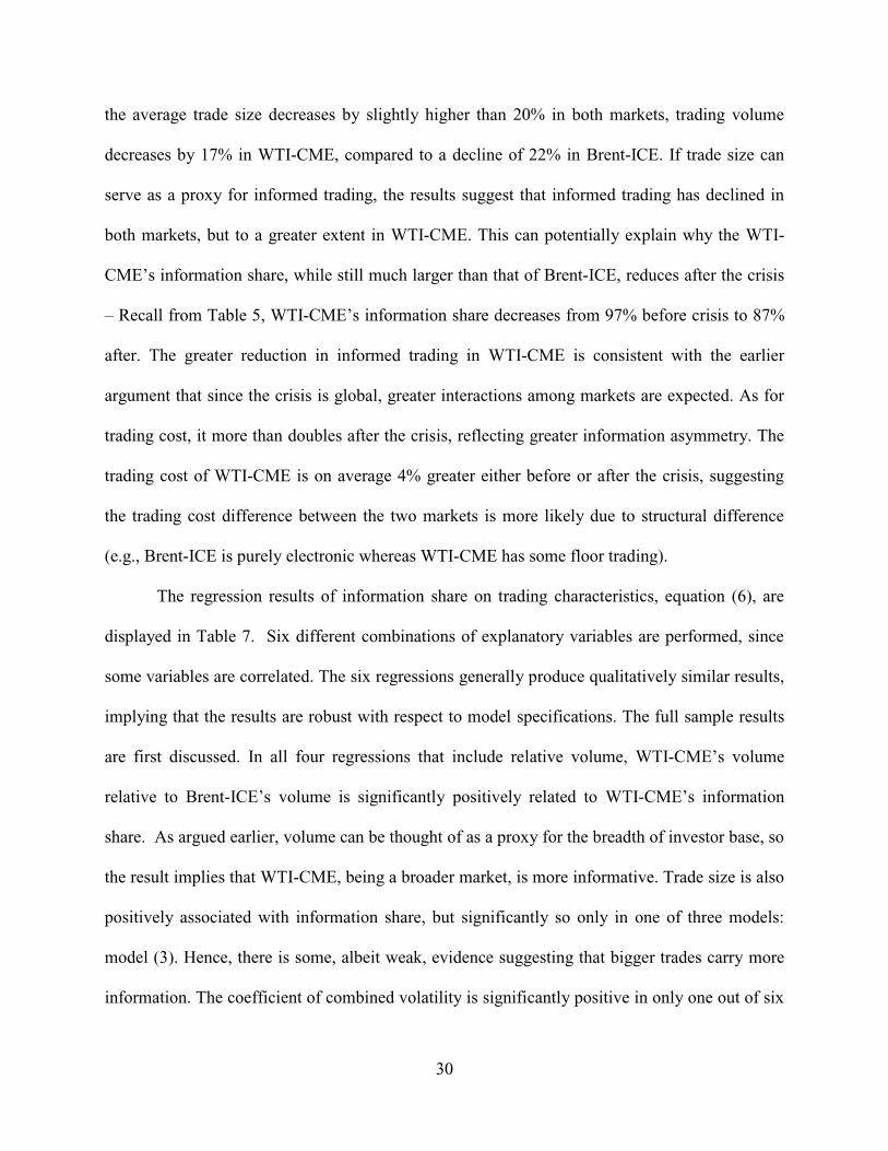
30

the average trade size decreases by slightly higher than 20% in both markets, trading volume

decreases by 17% in WTI-CME, compared to a decline of 22% in Brent-ICE. If trade size can

serve as a proxy for informed trading, the results suggest that informed trading has declined in

both markets, but to a greater extent in WTI-CME. This can potentially explain why the WTI-

CME’s information share, while still much larger than that of Brent-ICE, reduces after the crisis

– Recall from Table 5, WTI-CME’s information share decreases from 97% before crisis to 87%

after. The greater reduction in informed trading in WTI-CME is consistent with the earlier

argument that since the crisis is global, greater interactions among markets are expected. As for

trading cost, it more than doubles after the crisis, reflecting greater information asymmetry. The

trading cost of WTI-CME is on average 4% greater either before or after the crisis, suggesting

the trading cost difference between the two markets is more likely due to structural difference

(e.g., Brent-ICE is purely electronic whereas WTI-CME has some floor trading).

The regression results of information share on trading characteristics, equation (6), are

displayed in Table 7. Six different combinations of explanatory variables are performed, since

some variables are correlated. The six regressions generally produce qualitatively similar results,

implying that the results are robust with respect to model specifications. The full sample results

are first discussed. In all four regressions that include relative volume, WTI-CME’s volume

relative to Brent-ICE’s volume is significantly positively related to WTI-CME’s information

share. As argued earlier, volume can be thought of as a proxy for the breadth of investor base, so

the result implies that WTI-CME, being a broader market, is more informative. Trade size is also

positively associated with information share, but significantly so only in one of three models:

model (3). Hence, there is some, albeit weak, evidence suggesting that bigger trades carry more

information. The coefficient of combined volatility is significantly positive in only one out of six

31

models. As for trading cost, its coefficient is not significant in all four models that include this

variable. This is not consistent with some prior literature that suggests trading costs play an

important in information discovery. There are two possible explanations for the difference in

results. First, related studies do not directly estimate bid-ask spread, and most simply assume

bigger volume means greater liquidity. Recall that Table 6 finds WTI-CME actually has slightly

higher trading cost despite much greater volume, casting doubt about validity of that assumption.

Second, electronic trading has become dominant in recent years, and electronic trading tends to

be associated with lower trading costs, as some studies show. Hence it is possible that trading

cost might be relatively less important after mid-2000s. The R2 is not impressive; it is possible

that other factors such as history, tax structure, regulation, as well as geographic factors could

affect information share; unfortunately, these factors are hard to quantify.

32

Table 7: Regression Analysis of Share of Price Discovery

The table reports the regression estimate of West Texas Intermediate (WTI) light, sweet crude oil futures prices traded on CME (WTI-CME) price discovery share (θt

CME) on volume, trading cost,

trade size, and volatility. Volume is the relative volume, computed as the daily volume of the WTI-CME to the total volume of WTI-CME and Brent-ICE futures. TradeCost is the relative estimate of the effective bid ask spread of WTI-CME to Brent-ICE using the Gibbs estimator described in Hasbrouck (2004). Tradesize is the relative trade size defined as the trade size of WTI-CME to that of Brent-ICE futures. Volatility is an estimate of the daily volatility for WTI-CME futures (i.e., the daily sums the squares of intraday returns). The t-values are given in parentheses. The notations ―a‖, ―b‖ and ―c‖ refer to significance at 1, 5 and 10% level, respectively.

Dependent variable: WTI-CME futures contribution to price discovery (1) (2) (3) (4) (5) (6) Panel A :Full Sample

constant 0.052 0.099 0.244b 0.122 0.170 0.390a (0.33) (0.66) (2.38) (0.83) (1.22) (6.76) Volume 0.374c 0.372c 0.445b 0.444b (1.62) (1.61) (1.98) (1.98) TradeCost 0.045 0.044 0.046 0.045 (1.04) (1.02) (1.06) (1.04) Tradesize 0.094 0.095 0.122c (1.29) (1.31) (1.72) Volatility 0.061 0.067 0.107 0.068 0.073 0.128c (0.76) (0.83) (1.42) (0.84) (0.91) (1.71) R2 (%) 3.80 3.38 2.79 3.16 2.73 1.65 Panel B: Before financial crisis (Jan –Aug 2008) constant 0.137 0.126 0.070 0.267 0.252 0.226b (0.66) (0.64) (0.53) (1.36) (1.36) (2.30) Volume -0.130 -0.127 -0.075 -0.070 (-0.42) (-0.41) (-0.24) (-0.23) TradeCost -0.009 -0.008 -0.013 -0.013 (-0.17) (-0.14) (-0.25) (-0.23) Tradesize 0.138c 0.138c 0.134c (1.73) (1.74) (1.70) Volatility 0.860a 0.852a 0.812a 0.910a 0.899a 0.881a ( 2.91) (2.93) (2.99) (3.08) (3.08) (3.26) R2 (%) 7.71 7.69 7.61 6.04 6.01 6.01

33

Table 7 continued (1) (2) (3) (4) (5) (6) Panel C: After financial crisis (Sep - Dec 2008)

constant 0.030 0.119 0.396b -0.064 0.034 0.401a (0.13) (0.52) (2.02) (-0.29) (0.16) (3.49) Volume 1.042a 1.008a 0.837b 0.836b (2.79) (2.66) (2.50) (2.47) TradeCost 0.128c 0.119c 0.119c 0.119c (1.85) ( 1.65) (1.72) (1.67) Tradesize -0.202 -0.169 0.005 (-1.22) (-1.02) (0.03) Volatility -0.143 -0.099 -0.018 -0.171 -0.126 -0.016 (-0.94 (-0.65) (-0.12) (-1.13) (-0.83) (-0.11) R2 (%) 11.64 7.95 3.26 10.03 6.81 3.26

There are important differences between pre and post-crisis results, shown in Panels A

and B, respectively. Pre-crisis results in Panel B indicate two significant variables in all

regressions that include the two variables; namely, trade size and volatility are positively related

to information share. The former is consistent with Easley et al. (1987) that larger trades are

more informative. However, relative volume is not significant here. If one interprets the pre-

crisis period as relatively more ―normal‖, it might make sense that during a normal period, the

breadth of investor matters less than larger and more informative trades. In contrast, during

periods characterized by great uncertainty like the post-crisis period, the opposite might be true

since some big trades might come from panic or liquidity crunch. Indeed, Panel C post-crisis

results show that trade size is insignificantly related to information share but relative volume is.

Another great contrast between the two periods is that, after crisis, the coefficient of volatility is

insignificant in all regressions, suggesting that many trades might not be informative. It is

plausible that, in a chaotic market, trading is associated with a great degree of noise, and broader

34

investor base would matter more than other trading characteristics. Finally, in Panel C trading

cost is found to be positively correlated with information share in all four models that include it.

This piece of result is surprising and rather counter-intuitive. However, one could argue that

from the market maker’s standpoint, it makes sense to charge a greater spread for the more

informative market when the degree of uncertainty is large. To test the validity of this argument,

I use the Granger causality Wald tests to see if WTI-CME price discovery share (θtCME

) would

Granger cause the relative trading cost in the high volatility periods, i.e., the months after the

financial crisis.

Table 8 shows the Granger causality tests for the full sample as well as the two

subsamples. It is clear the relative trading cost Granger caused the WTI-CME price discovery

share in the full sample and in the months before the crisis. However, the Granger causality

shifts to indicate that WTI-CME price discovery share Granger caused the relative trading cost in

the months after the financial crisis, thus supporting the argument that, in periods of high

uncertainty, market makers would charge a greater bid-ask spread for the more informative

market.

35

Table 8: Granger Causality Wald Tests between Information Share and Trading Costs

The table reports the Granger causality Wald tests between the West Texas Intermediate (WTI) light, sweet crude oil futures prices traded on CME (WTI-CME) price discovery share (θt

CME)

and the relative trading cost (TradeCosttCME

) measured as the relative estimate of the effective bid ask spread of WTI-CME to Brent-ICE using the Gibbs estimator described in Hasbrouck (2004). The notations ―b‖ and ―c‖ refer to significance at 5 and 10% level, respectively.

TradeCosttCME θt

CME θtCME TradeCostt

CME

Panel A:

Full Sample chi2 9.347c 7.278 Prob > chi2 0.053 0.122 Panel B:

January – August 2008 chi2 12.838b 4.070 Prob > chi2 0.012 0.397 Panel C:

September- December 2008 chi2 3.231 10.383b Prob > chi2 0.520 0.034

7. Robustness of the Regression Analysis

To check the robustness of the regression results, I first use logistic transformation for

WTI-CME price discovery share (θtCME

) as ln(θtCME

/1- θtCME

). The logistic transformation for

θtCME is used as the dependent variable in equation (6). Eun and Sabherwal (2003) argue that this

logistic transformation is necessary to insure that the predicted regression value falls in the [0, 1]

range. The regression results using the logistic transformation for θtCME as dependent variable

are presented in Appendix A. This change does not alter the results.

36

Second, I use other proxies for the volatility: the Parkinson (1980) extreme value

volatility estimator and the Garman and Klass (1980) extreme value volatility estimator. The

extreme value volatility estimators are used since they tend to be more efficient during periods of

great volatility as in 2008, having alternative measures of volatility seems desirable.

Parkinson (1980) was first to propose an extreme value volatility estimator based upon

the joint density function of high (Ht) and low (Lt) prices at day t, following the Geometric

Brownian motion. He shows that his estimator is up to five times more efficient than the

traditional volatility estimator. Parkinson (1980)’s extreme value volatility estimator (VolP) can

be written as follows:

n

t

ttp LHn

Vol1

2)(ln2ln4

1. (15)

Garman and Klass (1980) suggest another extreme value volatility estimator

incorporating the opening (Ot) and the closing (Ct) prices, they show that this measure is

approximately up to 8.4 times more efficient than the traditional volatility estimator. Garman

and Klass (1980)’s extreme value volatility estimator (VolGK) is given by:

22 383.0)2)((019.0)(511.0 ttttttttGK CLHLHCLHVol . (16)

The regression results using Parkinson (1980)’s extreme value volatility estimator and

Garman and Klass (1980)’s extreme value volatility estimator as proxies for volatility do not

show any major changes from those in Table 7.

37

8. Conclusion

This paper empirically analyzes the effects of trading characteristics on the information

share of two major exchanges on crude oil, Chicago mercantile Exchange (CME) and

Intercontinental Exchange (ICE), using trade-by-trade data in 2008. The case of oil futures

market is interesting because oil is without doubt among the most important commodities and oil

futures is among the most liquid futures contracts in the world. The results should provide

implications for the role of trading characteristics on the relative leadership of markets. Trading

characteristics examined in the study include trading volume, trade size, and trading costs. In

contrast, most related studies analyze trading volume only. To estimate the information share, the

common factor components (CFC) model of Gonzalo and Granger (1995) is employed. As for

trading cost, since bid-ask spread data is unavailable, Hasbrouck (2004)’s spread estimator that

involves repeated sampling is utilized.

Another important objective of the study is to compare the periods before and after

September 2008, when the collapse of housing finance produced a global liquidity crunch. While

the crisis was not directly linked to the oil market, like other markets the oil market was affected

by the ensuing liquidity and confidence crisis; the rapid increase in oil price during summer 2008

might have contributed to or triggered the crisis.

Not too surprisingly, WTI-CME is characterized by greater trading volume and greater

average trade size, relative to Brent-ICE. Somewhat surprisingly, the bid-ask spread in WTI-

CME is on average 4% greater than that in Brent-ICE. An implication is that liquidity should not

be measured by one dimension or one variable alone. Nevertheless, WTI-CME’s overall liquidity

appears to be greater, as there is some evidence that it’s slightly higher trading cost might be due

38

to structural differences in trading systems. Not surprisingly, in 2008 the information share of

WTI-CME averages 87%, substantially greater than that of Brent-ICE’s 13%.

The information share of WTI-CME and trading characteristics that most affect

information share vary substantially between pre and post crisis periods. During the pre-crisis

period, relative trade size and volatility are positively related to WTI-CME’s information share.

The former is consistent with Easley and O’Hara (1987) theory that larger trades are more likely

to be motivated by private information. The greater number of large trades in CME is one reason

for the dominant information share of WTI-CME before the crisis: 97%. After the crisis,

however, WTI-CME’s share drops to 87%. Moreover, trade size is no longer a significant

explanatory variable for information share; rather, trading volume is. During liquidity crunch it is

reasonable to expect that trading might contain a great degree of noise thus trade size carries no

credible information. A broader market, as represented by greater volume, would be more

informative. The results are fairly robust, as different regression specifications and different

variable measurements produce virtually the same results.

As for trading costs, several studies suggest that they play an important role in

information discovery. Here the results contradict that conjecture. There are two possible

explanations. First, previous studies on futures market interactions do not estimate bid-ask spread

directly whereas this study does. Second, spread has been in a declining trend, especially after

the advancement of electronic trading systems. Finally, it is interesting to note in the post-crisis

period, spread is found to be significantly positively related to information share. A possible

explanation is that, during period of great uncertainty, market makers set greater spreads to more

informed market, as a protection for greater likelihood of adverse selection problem (i.e., trading

with more informed traders). Indeed, causality tests indicate that causality runs from spread to

39

information share before the crisis but the opposite conclusion holds during the post-crisis

period.

40

References

Amihud, Yakov and Haim Mendelson. 1986. Asset Pricing and the Bid-Ask Spread. Journal of

Financial Economics 17(2), 223-249. Andersen, Torben and Tim Bollerslev. 1998a. Deutsche Mark-Dollar Volatility: Intraday Activity Patterns, Macroeconomic Announcements, and Longer Run Dependencies. Journal of

Finance 53(1), 219– 265. Andersen, Torben and Tim Bollerslev. 1998b. Answering the Skeptics: Yes, Standard Volatility Models Do Provide Accurate Forecasts. International Economic Review 39(4), 885– 905. Ates, Aysegul and George H. Wang. 2005. Information Transmission in Electronic versus Open-Outcry Trading Systems: An Analysis of U.S. Equity Index Futures Markets. Journal of Futures

Markets 25(7), 67–9715 Baillie, Richard, Geoffrey Booth, Yiuman Tse and Tatyana Zabotina. 2002. Price Discovery and Common Factor Models. Journal of Financial Markets 5(3), 309-321. Bekaert, Geert, Campbell Harvey, and Christian Lundblad. 2007. Liquidity and Expected Returns: Lessons from Emerging Markets. Review of Financial Studies 20(6), 1783-1831. Brick, Ivan, Oded Palmon, and Dilip Patro. 2007. Stock Price Response to Calls of Convertible Bonds: Still a Puzzle? Financial Management 36(2), 1-21. Brunetti, Celso and Christopher Gilbert. 2000. Bivariate FIGARCH and Fractional Cointegration. Journal of Empirical Finance 7(5), 509-530 De Jong, Frank and Monique Donders. 1998. Intraday Lead-Lag Relationships between Futures, Options and the Stock Market. European Finance Review 1(3), 337–359. De Jong, Frank. 2002. Measures of Contributions to Price Discovery: A Comparison. Journal of

Financial Markets 5(3), 323-327. Easley, David and Maureen O'Hara. 1987. Price, Trade Size, and Information in Securities Markets. Journal of Financial Economics 19(1), 69-90. Engle, Robert and Clive Granger. 1987. Co-integration and Error Correction: Representation, Estimation, and Testing. Econometrica 55(2), 251—276. Eun, Cheol and Sanjiv Sabherwal. 2003. Cross-Border Listings and Price Discovery: Evidence from US-Listed Canadian Stock. Journal of Finance 58(2), 549-576.

Figuerola-Ferretti, Isabel and Jesús Gonzalo. 2010. Modeling and Measuring Price Discovery in Commodity Markets. Journal of Econometrics 158, 95-107.

41

Figuerola-Ferretti, Isabel and Jesús Gonzalo. 2009. Modeling and Measuring Price Discovery on the NYMEX and IPE Crude Oil Markets. Working Paper, Universidad Carlos III de Madrid. Fleming, Jeff, Barbara Ostdiek, and Robert Whaley. 1996. Trading Costs and the Relative Rates of Price Discovery in Stock, Futures, and Options Markets. Journal of Futures Markets 16(4), 353-387. Franke, Günter and Dieter Hess. 2000. Information Diffusion in Electronic and Floor Trading. Journal of Empirical Finance 7(5), 455–478. French, Kenneth and Richard Roll. 1986. Stock Return Variances: The Arrival of Information and the Reaction of Traders. Journal of Financial Economics 17(1), 5-26.

Fung, Joseph and Yiuman Tse. 2008. Efficiency of Single-Stock Futures: An Intraday Ananlysis. Journal of Futures Markets 28(6), 518-536. Gonzalo, Jesus and Clive Granger. 1995. Estimation of Common Long-Memory Components in Cointegrated Systems. Journal of Business and Economic Statistics 13(1), 27-36. Garman, Mark and Michael Klass. 1980. On the Estimation of Security Price Volatilities from Historical Data. The Journal of Business 53(1), 67-78. Harris, Frederick, Thomas McInish and Robert Wood. 2002. Security Price Adjustment across Exchanges: An Investigation of Common Factor Components for Dow Stocks. Journal of

Financial Markets 5(3), 277-308. Harris, Frederick, Thomas McInish, and Robert Wood. 2002. Common Factor Components versus Information Shares: A Reply. Journal of Financial Markets 5(3), 341-348.

Harris, Frederick, Thomas McInish, Gary Shoesmith, and Robert Wood. 1995. Cointegration, Error Correction, and Price Discovery on Informationally Linked Security Markets. Journal of

Financial and Quantitative Analysis 30(4), 563–579. Hasbrouck, Joel. 1995. One Security, Many Markets: Determining the Contribution to Price Discovery. Journal of Finance 50(4), 1175-1199. Hasbrouck, Joel. 2003. Intraday Price Formation in US Equity Index Markets. Journal of

Finance 58(6), 2375-2400. Hasbrouck, Joel. 2004. Liquidity in the Futures Pits: Inferring Market Dynamics from Incomplete Data. Journal of Financial and Quantitative Analysis 39(2), 305-326. Hsieh, Wen-Liang, Chin-Shen Lee, and Shu-Fang Yuan. 2008. Price Discovery in the Options Markets: An Application of Put-call Parity. Journal of Futures Markets 28(4), 354-375.

42

Johansen, Soren. 1988. Statistical Analysis of Cointegrating Vectors. Journal of Economic

Dynamics and Control 12(2-3), 231-254. Johnson, Timothy. 2008. Volume, Liquidity, and Liquidity Risk. Journal of Financial

Economics 87(2), 388-417. Kaufmann, Robert and Ben Ullman. 2009. Oil Prices, Speculation, and Fundamentals: Interpreting Causal Relations among Spot and Futures Prices. Energy Economics 31(4), 550-558.

Kim, Minho, Andrew Szakmary, and Thomas Schwarz. 1999. Trading Costs and Price Discovery across Stock Index Futures and Cash Markets. Journal of Futures Markets 19(4), 475-498. Martens, Martin. 1998. Price Discovery in High and Low Volatility Periods: Open Outcry versus Electronic Trading. Journal of International Financial Markets, Institutions and Money 8(3-4), 243-260. McLean, David R. 2010. Idiosyncratic Risk, Long-Term Reversal, and Momentum. Journal of

Financial and Quantitative Analysis 45(4), 883-906. Moosa, Imad. 2002. Price Discovery and Risk Transfer in the Crude Oil Futures Market: Some Structural Time Series Evidence. Economic Notes 31(1), 155-165.

Parkinson, Michael. 1980. The Extreme Value Method for Estimating the Variance of the Rate of Return. Journal of Business 53(1), 61-65. Rangel, Jose. 2005. Macroeconomic Announcements, Price Discovery, and Order Flow Effects in the Stock Market: Evidence from Incomplete Data and Multiple Financial Markets. Working paper, University of California, San Diego Rappaport, Daniel. 2000. Price Discovery and Energy Risk, or How Futures Contracts are Changing the Energy Markets Forever: The Case of the New York Mercantile Exchange. The

Journal of Risk Finance 1(4), 33-42. Roll, Richard. 1984. A Simple Implicit Measure of the Effective Bid-ask Spread in an Efficient Market. Journal of Finance 39(4), 1127-1139. Schlusche, Bernd. 2009. Price Formation in Spot and Futures Markets: Exchange Traded Funds vs. Index Futures. The Journal of Derivatives 17(2), 26-40. Schwarz, Gideon. 1978. Estimating the Dimension of a Model. Annals of Statistics, 6, 461-464. Schwarz, Thomas and Andrew Szakmary. 1994. Price Discovery in Petroleum Markets: Arbitrage, Cointegration, and the Time Interval of Analysis. Journal of Futures Markets 14(2), 147-167.

43

Shastri, Kuldeep, Ramabhadran Thirumalai, and Chad Zutter. 2008. Information Revelation in the Futures Market: Evidence from Single Stock Futures. Journal of Futures Markets 28(4), 335-353. Silvapulle, Param and Imad Moosa. 1999. The Relationship between Spot and Futures Prices: Evidence from the Crude Oil Market. Journal of Futures Markets 19(2), 175–193. Skouratova, Elena, Yiuman Tse, and Valeria Martinez. 2008. Market competition in crude oil futures. Working Paper, Department of Finance, University of Texas at San Antonio. Smith, Tom and Robert E. Whaley. 1994. Estimating the Effective Bid/Ask Spread from Time and Sales Data. Journal of Futures Markets 14(4), 437-455. Stoll, Hans. R. 2000. Friction. Journal of Finance 55(4), 1479-1514.

Theissen, Erik. 2002. Price discovery in floor and screen trading systems. Journal of Empirical

Finance 9(4), 455-474. Thompson, Sarahelen and M. L. Waller. 1988. Determinants of Liquidity Costs in Commodity Futures Markets. Review of Futures Markets 7(1), 110-126. Tse, Yiuman and Paramita Bandyopadhyay. 2006. Multi-Market Trading in the Eurodollar Futures Market. Review of Quantitative Finance and Accounting 26(3), 321-341. Tse, Yiuman and Tatyana Zabotina. 2004. Do Designated Market Makers Improve Liquidity in Open-Outcry Futures Markets? Journal of Futures Markets 24(5), 479-502. Tse,Yiuman, Paramita Bandyopadhyay, and Yang-Pin Shen. 2006. Intraday Price Discovery in the DJIA Index Markets. Journal of Business Finance and Accounting 33(9-10), 1572-1585.

44

Appendix A

Regression Analysis of Share of Price Discovery

The table reports the daily regression estimate the logistic transformation of West Texas Intermediate (WTI) light, sweet crude oil futures prices traded on CME (WTI-CME) price discovery share (θt

CME) on volume, trading cost, trade size, and volatility. Volume is the relative

volume, computed as the daily volume of the WTI-CME to the total volume of WTI-CME and Brent-ICE futures. TradeCost is the relative estimate of the effective bid ask spread of WTI-CME to Brent-ICE using the Gibbs estimator described in Hasbrouck (2004). Tradesize is the relative trade size defined as the trade size of WTI-CME to that of Brent-ICE futures. Volatility is an estimate of the daily volatility for WTI-CME futures (i.e., sums the squares of intraday returns). The total number of daily observations is 257. The t-values are given in parentheses. The notations ―a‖, ―b‖ and ―c‖ refer to significance at 1, 5 and 10% level, respectively.

Dependent variable: logistic transformation of WTI-CME futures contribution to price discovery (1) (2) (3) (4) (5) (6) Panel A :Full Sample

constant -2.895a -2.640a -1.572a -2.471a -2.207a -0.660b (-3.31) (-3.15) (-2.74) (-3.01) (-2.83) (-2.04) Volume 2.580b 2.567b 3.009b 3.001b (2.00) (1.99) (2.40) (2.39) TradeCost 0.245 0.241 0.250 0.246 (1.02) (0.99) (1.04) (1.01) Tradesize 0.568 0.574 0.760b (1.40) (1.42) (1.92) Volatility 0.416 0.446 0.732c 0.455 0.486 0.862b (0.93) (1.00) (1.73) (1.01) (1.09) (2.06) R2 (%) 5.06 4.67 3.55 4.32 3.91 2.15 Panel B: Before financial crisis (Jan –Aug 2008) constant -2.922 -2.904b -2.641a -2.097c -2.110 -1.609a (-2.46) (-2.58) (-3.48) (-1.88) (-2.00) (-2.88) Volume 0.547 0.541 0.896 0.901 (0.31) (0.31) (0.51) (0.51) TradeCost 0.016 0.010 -0.012 -0.022 (0.05) (0.03) (-0.04) (-0.07) Tradesize 0.878b 0.877b 0.892b (1.94) (1.94) (1.98) Volatility 4.277b 4.289b 4.477a 4.597a 4.588a 4.937a ( 2.55) (2.59) (2.90) (2.73) (2.76) (3.21) R2 (%) 8.09 8.09 8.04 6.00 6.00 5.86

45

Appendix A continued

Dependent variable: logistic transformation of WTI-CME futures contribution to price discovery (1) (2) (3) (4) (5) (6) Panel C: After financial crisis (Sep - Dec 2008)

constant -2.390c -1.939 -0.401 -2.904b -2.411b -0.380 (-1.91) (-1.56) (-0.37) (-2.45) (-2.09) (-0.61) Volume 0.059a 5.498a 4.545b 4.543b (2.78) (2.66) (2.48) (2.46) TradeCost 0.651c 0.599 0.601c 0.600 (1.72) (1.53) (1.59) (1.55) Tradesize -1.107 -0.940 0.020 (-1.23) (-1.04) (0.02) Volatility -0.820 -0.599 -0.141 -0.973 -0.744 -0.135 (-0.98) (-0.72) (-0.17) (-1.18) (-0.90) (-0.17) R2 (%) 11.14 7.93 2.78 9.51 6.74 2.78

46

Appendix B

Correlation Matrix

Volume is the relative volume, computed as the daily volume of the WTI-CME to the total volume of WTI-CME and Brent-ICE futures. TradeCost is the relative estimate of the effective bid ask spread of WTI-CME to Brent-ICE using the Gibbs estimator described in Hasbrouck (2004). Tradesize is the relative trade size defined as the trade size of WTI-CME to that of Brent-ICE futures. Volatility is an estimate of the daily volatility for WTI-CME futures (i.e., sums the squares of intraday returns).

Volume TradeCost Tradesize Volatility

Panel A :Full Sample

Volume 1.000 TradeCost 0.021 1.000

Tradesize 0.278 0.024 1.000 Volatility 0.379 0.070 0.162 1.000

Panel B: Before financial crisis (Jan –Aug 2008)

Volume 1.000 TradeCost -0.012 1.000

Tradesize 0.153 -0.033 1.000 Volatility 0.395 0.125 0.145 1.000

Panel C: After financial crisis (Sep - Dec 2008)

Volume 1.000 TradeCost 0.078 1.000

Tradesize 0.526 0.154 1.000 Volatility 0.414 0.189 0.348 1.000

47

Chapter 2

Factors Affecting Backwardation in Crude Oil Futures Price

Introduction

Backwardation is a market condition in which futures prices is lower than the spot price

for a certain commodity. For crude oil, Litzenberger and Rabinowitz (1995) observe that oil

futures prices are often backwardated; specifically they find that strong backwardation -- futures

price less than the spot price -- occurs 77% of the time in oil futures markets, while weak

backwardation -- discounted oil futures price less than the spot price -- occurs 94% of the time

over the period of February 1984 through April 1992. Knetsch (2007) also confirms

Litzenberger and Rabinowitz (1995) observation, that oil market is weakly backwarded in most

cases11

.

Using on the supply/demand argument, backwardation occurs when unexpected supply

shortage appears, causing a short-term upward price movement. In this case, consumers pay a

premium to take delivery of commodities right away to ensure a security level for the

commodity. This will raise spot price directly by shifting the demand curve upward given a

vertical supply curve.

The main goal of this study is to examine the influence of expected oil price volatility,

the behavior of the Organization of Petroleum Exporting Countries (OPEC), and the US Dollar

11

According to Knetsch’s observation there were two periods in which oil futures did not exhibit backwardation. The first period was around the winter 1998–1999, and the second period in the summer of 2004 until the end of his sample period of 2006.

48

exchange rate volatility on oil futures backwardation. Both Dollar value12

and OPEC behavior

are believed to be important factors affecting oil price; this study hypothesizes that they also

affect the relation between spot and futures prices of oil, since uncertainties about exchange rate

and OPEC policies (and deviations from them) increase the uncertainties about future

supply/demand, thus altering the connection between spot and futures prices. With regard to

exchange rate, the paper incorporates the effects of the volatility of the US exchange rate on

crude oil backwardation. As for the role of OPEC behavior, the study examines OPEC

production quota imposed on its members and OPEC member’s overproduction (difference

between quota and the actual production). Additionally, the impact of oil fund activity is

examined; since oil funds are relatively new however, the analysis involving oil fund activity

utilizes a much shorter sample period. Studying these factors can improve our understanding of

the spot-futures relation. To my knowledge, there is no similar study that incorporates these

factors as potential explanations for backwardation in the oil market.

As for the role of oil price volatility, Litzenberger and Rabinowitz (1995) offer an

explanation for the backwardation in oil futures based on the option pricing theory13

. They argue

that backwardation of crude oil prices is a necessary condition for crude oil production and that

greater uncertainty regarding future crude oil prices will lead to a stronger backwardation.

Specifically, Litzenberger and Rabinowitz (1995) view crude oil reserve as a call option written

on the spot price of oil with the strike price equal to the extraction cost. Option pricing theory

predicts that option value is greater the greater the volatility of the underlying asset. In

equilibrium, their theory predicts a negative association between production and oil price

12

The US Dollar has been the major currency used in oil transactions. 13

The earliest option pricing model that derives a closed-form solution for option is due Black and Scholes (1973).

49

volatility; this is because the value of the oil reserve is greater the greater the price volatility.

Consequently when price volatility is higher, the value of oil reserve is higher, thus production is

typically lower and backwardation must be greater to encourage current production. That is, their

theory predicts a positive association between backwardation and volatility.

Other related studies on backwardation analyze the notion of convenience yield (see

Kaldor; 1939, Working; 1948) and the supply/demand imbalances (see Alquist and Kilian; 2010

and Milonas and Henker; 2001) as potential explanations for backwardation in futures prices of

storable commodities. The convenience yield is defined as an implicit dividend that accrues to

the holder of the commodity. In sum, previous studies examine several factors that explain the

crude oil price backwardation, including supply/demand uncertainty, price volatility, seasonality,

and maturity. However, none of these studies took into consideration the effects of the US

Dollar exchange rate volatility and OPEC’s behavior.

Given that crude oil is one of the most essential energy sources and that there is

considerable fluctuation in oil supply, which depends on a variety of macroeconomic and

political factors, crude oil market has witnessed high volatility. For example, in 1997, when the

world economy was already in a recession, OPEC failed to predict the oil demand correctly and

increased its production levels that resulted in a huge decrease in oil prices. In June-July 2008, a

combination of supply uncertainties in oil producing countries and a falling US Dollar caused an

unprecedented oil price spike. Horan, Peterson, and Mahar (2004) examine the behavior of

crude oil implied volatility surrounding OPEC meetings, their results show that volatility drifts

upward as the meeting approaches. The implied volatility is the volatility implied from the

50

market price of an option on oil, based on an option pricing model14. On the reverse, an

appreciation of the US Dollar and signs of worldwide economic slowdown led to a sharp

decrease in oil price toward the end of 2008. In fact, the US Dollar exchange rate is a key

determinant of the world oil markets because world oil prices are denominated in US Dollars, a

stronger Dollar pushes up world oil prices measured in local currencies, even if the Dollar price

is unchanged. Conversely, when the Dollar falls, OPEC members receive smaller revenues in

terms of their domestic currencies, causing substantial cuts in their purchasing power.

The remainder of this paper is organized as follows. In section one I provide more

systematic review of the related literature. Section two describes the data. Section three

discusses oil backwardation. Section four discusses the potential role of expected oil price

volatility, OPEC behavior, and the US Dollar exchange rate volatility on the backwardation of

crude oil futures. Section five concludes.

1. Literature Review

There are two well-known theories of the relationship between the futures and the spot

prices; the theory of storage and the theory of normal backwardation. The theory of storage was

initially developed by Kaldor (1939) and Working (1949). According to the theory of storage,

the difference between contemporaneous spot and futures prices is explained by the following

factors: the interest rate in storing a commodity, storage costs, and convenience yield. This can

be expressed as:

14

The most well-known implied volatility is so called the VIX index, which represents the implied volatility of S&P 500 stocks. It is computed from the market price of options on S&P 500 stocks. The VIX index is published daily in financial media.

51

TtTtTtttTt ycrSSF ,,,, )( , (1)

where Ft,T is the price of futures at time t for delivery at time T. St is the spot price at time t. rt is

the interest rate. ctT is the marginal cost of storage. ytT is the marginal convenience yield.

Accordingly a high inventory level implies a lower probability of a stock-out in the future, that

is, convenience yields are negatively related to inventory levels. This relationship is stronger for

a commodity that is more sensitive to seasonality or supply/demand effect. Therefore,

convenience yield plays a central role in explaining the benefits of holding inventory during

periods of unexpected demand/supply shock. Fama and French (1987, 1988) perform tests on the

theory of storage and present empirical evidence that in periods of increasing volatility and risk,

convenience yields increase for a wide variety of metals prices (aluminum, copper, nickel, and

lead).

Another view of commodity futures is the theory of normal backwardation, which

compares futures prices to expected future spot prices. The theory of normal backwardation

views futures markets as a risk transfer mechanism between long investors earn a risk premium

for bearing future spot risk and the commodity producers who want to hedge. This theory builds

on the view that the basis consists of two components: a risk premium and the expected

appreciation or depreciation of the future spot price.

According to the theory of normal backwardation, deviations of futures prices from

expected future spot prices stem from a risk premium, which arises if long or short traders are

more risk-averse than their counterparts. It is generally accepted that futures markets provide

insurance to hedgers by ensuring the transfer of price risk to speculators. The insurance that net

hedgers are willing to pay equals to the premium earned by speculators for this risk bearing. If

52

long hedgers are more risk averse than their counterparts, futures prices would lie above the

expected future spot price and the long hedgers would have to pay a premium to induce short

traders into taking opposite position in the future. This situation is referred as contango. On the

other hand, if short traders are more risk averse than their counterparts, futures prices would lie

below the expected future spot price and the short hedger pays a premium for being able to shift

risk burden to the opposite party. This situation is referred to as normal backwardation.

Backwardation in crude oil prices is inconsistent with Hotelling's (1931) theory.

Hotelling (1931) derived the commonly used rule to determine the optimal extraction time-path

for a non-renewable resource. Hotelling's rule states that under certainty the net price of an

exhaustible resource rises over time at the rate of interest. The rationale is that if prices would

move differently, it would be worthwhile to shift production between periods. This is the

simplest and most commonly cited form of Hotelling's rule and uses. However, in Hotelling's

simplest model specification, price and net price can be interchangeably used because extraction

costs are assumed to be zero. Hence price is equal to net price (price minus marginal cost) given

that marginal extraction cost is zero by assumption.

Its existence, which has attracted considerable attention, represents a puzzle because of

the violation of the optimal inter-temporal inventory holding under certainty. Empirical tests of

the Hotelling’s theory include testing the relationship between growth in mineral prices and

interest rate (e.g., see Heal and Barrow, 1980; Smith, 1981). In general the results of these tests

have not been strongly supportive. In petroleum, Cairns and Davis (2001), Thompson (2001),

Adelman (1991), and Adelman and Watkins (2005) test the theory using reserve data from US

petroleum reserve transactions. They find that the empirical evidence is not consistent with the

53

predictions of the Hotelling’s theory; they argue that the Hotelling’s theory cannot hold under

uncertainties.

Litzenberger and Rabinowitz (1995) develop a model based on the option pricing theory.

In their model, oil reserve is viewed as a call option on oil, and therefore its value is greater the

greater the oil price volatility (based on the option pricing theory). They view backwardation as

the price to pay for the producers to refrain from keeping oil in the ground. Prior to Litzenberger

and Rabinowitz (1995) theory, no model had predicted any association between backwardation

and volatility. They argue that backwardation of crude oil prices is a necessary condition for

crude oil production and greater uncertainty regarding future crude oil prices will lead to stronger

backwardation because greater uncertainty means higher value of oil reserve (i.e., greater

tendency to keep oil in the ground). Stated differently, Litzenberger and Rabinowitz (1995)

model considers the effects of oil price volatility and examines the relation between volatility

and the slope of the forward curve. When volatility is high, the value of delaying production

increases, causing current prices to increase relative to future prices. Their model implies that,

when riskiness increases, oil production is non-increasing and inter-temporal oil price spreads

are non-decreasing. In specific, their theory predicts a positive association between

backwardation and volatility. Regressing weak backwardation on the implied volatility of the at-

the-money put option price using the Black (1976) formula, Litzenberger and Rabinowitz (1995)

using data on U.S. oil production, U.S. oil reserves, and west Texas intermediate futures and

options prices show that the coefficient on implied volatility is significantly positive over the

period from December 1986 through December 1991.

Brennan and Schwartz (1985) as well as Gibson and Schwartz (1990) study the marginal

convenience yield; they argue that backwardation should be equal to the present value of the

54

marginal convenience yield of the commodity inventory. The convenience yield is the benefit of

owning the physical asset and it measures the market’s expectations about the future availability

of the commodity. The higher the perceived risk of future shortages in supply, the higher the

convenience yield. If the convenience yield is high enough and exceeds the cost of carry, the

future market is likely to shift into backwardation. With a low or negative convenience yield, the

future market is likely to stay in contango.

Brennan and Schwartz (1985) and Gibson and Schwartz (1990) derive the market price

for pricing petroleum assets based on the observable term structure of petroleum futures markets.

Although motivated by the time series properties of the forward convenience yield of crude oil,

Gibson and Schwartz (1990) developed an empirical model of pricing assets, which explicitly

model a risk-premium based on stochastic price movements. They use the adjacent monthly

maturities futures prices and annualized riskless interest rate between January 1984 and

November 1988 to compute the implied convenience yield that is not directly observable. Their

results show that the stochastic convenience yield has a strong mean reversing tendency.

Larson (1994) develops a stochastic arbitrage equation to explain backwardation in

refined copper. Extending on Larson (1994) work, Considine and Larson (2001) show that the

equilibrium value of oil inventory contains: the conventional Hotelling’s theory, the convenience

yield from the theory of storage, and an option value related to price uncertainty. Their results

suggest that convenience yield and risk premium are important elements of crude oil

backwardation. In fact, Carlson, Khokher, and Titman (2007) develop a model related to

Litzenberger and Rabinowitz (1995) model. In their model they relax Litzenberger and

Rabinowitz (1995) assumption that producers are not able to extract all of an oil well’s reserves

at an arbitrary point. Carlson et al. (2007) analysis shows that volatility of price changes can

55

arise as a natural consequence of the production decisions made by value maximizing resource

owners and that this volatility is related to the extent of backwardation as well as contango

(futures price greater than spot price).

Milonas and Henker (2001) argue that backwardation could be explained by supply and

demand imbalances. They model the Brent crude oil and West Texas Intermediate (WTI) futures

spread as a function of the convenience yields of the two contracts. They use convenience yields

as surrogates for supply and demand conditions in the two markets and find that convenience

yields can explain the variation in the spread. This indicates that the regional supply and demand

imbalance is an important factor in determining oil futures prices. In a recent study, Alquist and

Kilian (2010) also view supply and demand imbalance as an explanation of oil futures

backwardation. They show that the overshooting of the price of oil in response to oil-market

specific demand shocks coincides with the predictions of theoretical models of precautionary

demand shocks driven by increased uncertainty about future oil supply shortfalls. Using oil

futures market data since 1989, Alquist and Kilian (2010) show that the movements in the price

of oil induced by this shock are highly correlated (as high as 80%), with independent measures

of the precautionary demand component of the real price of oil based on crude oil futures prices.

Another important supply side factor is the behavior of OPEC-countries. OPEC uses

several instruments to control the oil market. Since 1983 OPEC has announced the production

quota of all its member countries in an attempt to stabilize crude oil prices by controlling oil

production.15

OPEC uses eight criteria, that are oil related factors and socio-economic, for

allocating quotas. These include the following: oil reserves, production capacity, historical

15 Over the years, the OPEC quota system has essentially never worked, since OPEC has no way to enforce

compliance by its members, and because there were always member’s dissatisfied with their assigned quotas.

That’s why oil production by OPEC members generally exceeded the production ceiling.

56

production share, domestic oil consumption, population, dependence on oil exports, and external

debt.

Moebert (2007) find a modest influence of OPEC’s capacity utilization on crude oil. His

findings imply that the upward trend at the spot market can be explained by an increasing crude

oil demand of emerging markets rather than OPEC’s market power. In fact, he views OPEC as a

passive observer than a price setter. The findings of Moebert (2007) are unlike Kaufmann et al.

(2004) who study OPEC behavior between 1984 and 2002 using data on OPEC quota (defined as

the quantity of oil to be produced by OPEC members), OPEC overproduction (the quantity of oil

produced minus the OPEC quota), and capacity utilization. They show that OPEC can influence

real oil prices, while their econometric specification can produce accurate in-sample static and

dynamic forecasts. Horan, Peterson, and Mahar (2004) examine the behavior of crude oil

implied volatility surrounding OPEC meetings, and their results show that volatility drifts

upward as the meeting approaches. Similarly, Wang, Wu, and Yang (2008) show that the

realized crude oil futures volatility responds with an increase in the weeks immediately before

the OPEC events recommending price increases.

2. Data

The study uses West Texas International (WTI) light, sweet crude oil futures to analyze

the impacts of oil volatility, OPEC behavior, and the US Dollar exchange rate volatility on

backwardation during the period from January 1986 to December 2008. WTI futures data are

obtained from the US Energy Information Administration.16

The futures data include the four

16 www.eia.doe.gov

57

shortest maturity contracts from 1-month to 4-months.17

The futures prices are the official daily

closing prices at 2:30 p.m. from the trading floor of the New York Mercantile Exchange

(NYMEX) for a specific delivery month for each product listed. Each contract expires on the

third business day prior to the 25th calendar day of the month proceeding the delivery month. If

the 25th calendar day of the month is a non-business day, trading ceases on the third business day

prior to the business day proceeding the 25th calendar day.

Table 1: Summary Statistics of Futures Prices

The table summarizes the daily logarithm of the 1-month, 2-month, 3-month, and 4-month West Texas Intermediate (WTI) light, sweet crude oil futures price series from January 1986 to December 2008. WTI futures daily data are obtained from the US Energy Information Administration. The notation ―a‖ refers to significance at 1% level.

1-month

futures

2-month futures

3-month

futures

4-month futures

Mean 3.265 3.261 3.257 3.253

Variance 0.292 0.294 0.295 0.296

Minimum 2.344 2.355 2.359 2.371

Maximum 4.979 4.983 4.984 4.987

Skewness 1.110a 1.142a 1.175a 1.208a

Kurtosis 3.458a 3.471a 3.500a 3.539a

No. of observations

5,708 5,708 5,708 5,708

17

The 1-month futures contract is the nearest to maturity contract and its time to expiration ranges from one day to thirty one days. The 2-month contract has one additional month to expiration. The 3-month has two additional months, etc.

58

Table 1 provides summary statistics of the four months logarithm daily futures price

series. The total number of observations is 5,708 spanning from January 1986 to December

2008. It can be seen that the mean value for the logarithm futures price decreases as the month

of maturity increased. The price series in all four maturity contacts show statistically significant

positive kurtosis, indicating a leptokurtic, or fat tail.

3. Oil Backwardation

As discussed above crude oil futures prices are often backwardated (Knetsch, 2007 and

Litzenberger and Rabinowitz, 1995). Table 2 presents a summary statistics of strong and weak

backwardation for the WTI futures with maturity contracts for two-month, three-month and four-

month contracts. Strong backwardation SBt is defined as the spot price being higher than the

futures price:

0, tntt FSSB , (2)

where St is the price of the 1-month futures contract (which is used as a proxy for the spot price),

Fn,t is the price of the n-th month futures contract. Weak backwardation WBt is defined as the

spot price being higher than the discounted futures price:

0,

tn

nr

tt FeSWB t ,

(3)

where r is the 3-month Treasury bill. From Table 2, it can be seen that the level of backwardation

is higher for the far month’s futures contracts than that of the nearby futures contracts. For

example, the level of strong backwardation of 2-month futures contract is $0.261, while the

backwardation level for the 3-month and 4-month futures are $0.445 and $0.643, respectively.

59

Furthermore, the values of weak backwardation are $0.06, $0.145, and $0.246 for the 2-month,

3-month, and 4-month futures contracts, respectively. This is also true for the fraction of time

futures prices are backwardated: being higher for the far month’s futures than the nearby

contracts. The table shows that oil futures contracts are, on average, strongly backwardated 57%

of the time and weakly backwardated 69% of the time during the period from January 1986 to

December 2008.

Table 2: Summary Statistics of Oil Backwardation

The table reports a summary statistics of the strong and weak backwardation of the 1-month, 2-month, 3-month, and 4-month West Texas Intermediate (WTI) light, sweet crude oil futures price series from January 1986 to December 2008. Strong backwardation is measured as the difference between the price of the 1-month futures contract (proxy of spot price) and the futures price of the n-th month futures contract. Weak backwardation is measured as the difference between the price of the 1-month futures contract and discounted futures price of the n-th month futures contract.

Futures contract 2-month 3-month 4-month

Panel A: strong backwardation ($)

Mean 0.261 0.445 0.643 Standard Deviation 0.686 1.132 1.491 Median 0.209 0.391 0.575 Minimum -8.489 -11.288 -13.277 Maximum 11.785 12.401 12.607 Panel B: weak backwardation ($)

Mean 0.060 0.145 0.246 Standard Deviation 0.702 1.163 1.537 Median 0.050 0.160 0.260 Minimum -8.490 -11.290 -13.280 Maximum 11.550 12.050 12.140 Panel C: Fraction of the Time in Backwardation (in%) Strong 54.61 57.38 59.95 Weak 67.71 68.62 70.41

60

Figures 1-A, 1-B, 1-C, 2-A, 2-B, and 2-C display the spot price vs. the strong and weak

backwardation of the 2-month, 3-month and 4-month futures contracts, respectively. As shown

from these figures, the market experiences backwardation between 1986 and 2004, while it has

some prolong periods of contango (which lasted more than 12 months) in 1998 and between

February 2005 to June 2007.

Figure 1:Crude Oil Spot Price and Strong Backwardation in Oil Futures

(January 1986 – December 2008)

The figures 1-A, 1-B, and 1-C show the daily futures price for the 1-month futures contract, a proxy for the spot price, and the strong backwardation of the 2-month, 3-month and 4-motnh futures contracts. Strong backwardation is measured as the difference between the price of the 1-month futures contract (proxy of spot price) and futures price of the n-th month futures contract.

(A) Spot price and strong backwardation of the 2-month WTI crude oil futures contract.

-16

-12

-8

-4

0

4

8

12

16

0

20

40

60

80

100

120

140

160

86 88 90 92 94 96 98 00 02 04 06 08

$$

Spot Price

Strong Backwardation

61

(B) Spot price and strong backwardation of the 3-month WTI crude oil futures contract.

(C) Spot price and strong backwardation of the 4-month WTI crude oil futures contract.

-20

-15

-10

-5

0

5

10

15

20

0

20

40

60

80

100

120

140

160

86 88 90 92 94 96 98 00 02 04 06 08

$$

Spot Price

Strong Backwardation

-20

-15

-10

-5

0

5

10

15

20

0

20

40

60

80

100

120

140

160

86 88 90 92 94 96 98 00 02 04 06 08

$$

Spot Price

Strong Backwardation

62

Figure 2: Crude Oil Spot Price and Weak Backwardation in Oil Futures

(January 1986 – December 2008)

The figures 2-A, 2-B, and 2-C show the daily futures price for the 1-month futures contract, a proxy for the spot price, and the weak backwardation of the 2-month, 3-month and 4-motnh futures contracts. Weak backwardation is measured as the difference between the price of the 1-month futures contract (proxy of spot price) and discounted futures price of the n-th month futures contract.

(A) Spot price and weak backwardation of the 2-month WTI crude oil futures contract.

-16

-12

-8

-4

0

4

8

12

16

0

20

40

60

80

100

120

140

160

86 88 90 92 94 96 98 00 02 04 06 08

$$

Spot Price

Weak Backwardation

63

(B) Spot price and weak backwardation of the 3-month WTI crude oil futures contract.

(C) Spot price and weak backwardation of the 4-month WTI crude oil futures contract.

-20

-15

-10

-5

0

5

10

15

20

0

20

40

60

80

100

120

140

160

86 88 90 92 94 96 98 00 02 04 06 08

$$

Weak Backwardation

Spot Price

-20

-15

-10

-5

0

5

10

15

20

0

20

40

60

80

100

120

140

160

86 88 90 92 94 96 98 00 02 04 06 08

$$

Spot Price

Weak Backwardation

64

The contango period of 1998 was associated with a declining trend of the crude oil prices.

This is consistent with the conventional wisdom that in periods of contango oil producers

accumulate inventories that is interpreted by the market participants as an increase of crude oil

supply relative to demand. This would result in pushing the price of oil for immediate delivery to

go down. Contrary to this notion, the 2005-2007 contango period was associated with an upward

trend in oil prices despite of the rise of inventories. Morse (2006) argues that high levels of

inventories are no longer seen as a necessary sign of oversupply. Furthermore, Fattouh (2007)

argues that this transformation is due to the absence of spare capacity, and the decline in oil price

caused by rising inventories is continuously being dominated by other factors causing oil prices

to rise.

4. Factors Affecting Backwardation

The study examines the influence of oil price volatility, the behavior of OPEC, and the

US Dollar exchange rate volatility, on the backwardation of crude oil futures. The extent of oil

strong and weak backwardation is used as the dependent variable in a regression analysis.

The study variables of main interest are volatility, quota, over, and Dollar_vol, where

volatility is the realized volatility of crude oil futures, quota is the OPEC crude oil production

ceiling allocation measured in 1,000 barrel/day, over is the OPEC overproduction rate defined as

the actual production rate minus OPEC quota measured in 1,000 barrel/day, and Dollar_vol is

the volatility of the US Dollar exchange rate against the British Pound and Japanese Yen. The

regression is estimated using the White (1980) correction to account for heteroskedasticity.

65

Figure 3: OPEC Crude Oil Production and Quota

The figure shows the monthly average crude oil production by Organization of Petroleum Exporting Countries (OPEC), measured in 1,000 barrel/day, and the OPEC crude oil production ceiling, measured in 1,000 barrel/day, during January 1999 – December 2008. Monthly data are obtained from OPEC annual statistical reports (2002-2009).

To test the impact of OPEC polices on oil price backwardation, the study employs two

variables: OPEC crude oil production allocation to its members, quota, and OPEC

overproduction rate by its members, Over.18

The daily and monthly data for these variables are

obtained from OPEC annual statistical bulletin from 2002 to 2008. Figure 3 shows that the

monthly average of the actual oil production always exceeds the agreed production ceiling

allocation during January 1999 to December 2008. On average, the overproduction is around 3

18

The monthly data for the actual OPEC production rate is only available from January 1999.

20000

22000

24000

26000

28000

30000

32000

34000

99 00 01 02 03 04 05 06 07 08

OPEC crude oil production

OPEC crude oil production ceiling allocations

1,0

00

b/d

66

million barrel/day, which is 12% above the average quota. It can be argued that this deviation

will discourage current oil production and result in greater backwardation levels.

Litzenberger and Rabinowitz (1995) test their theory by regressing weak backwardation

on the implied volatility of the at-the-money put option price using the Black (1976) formula.

Theoretically, implied volatility reflects option traders’ collective estimate of what volatility will

be during the life of an option contract. This study does not use implied volatility, since data on

oil options is unavailable to the author. Additionally, studies such as Martin, Reidy, and Wright

(2009), Neely (2009), and Martens and Zein (2004) find that implied volatility is not a superior

forecaster of future volatility, compared to historical volatility. Moreover, since volatility is time-

varying, it is entirely possible that investors might place more weight on recent volatility than on

volatility in the distant past (based on behavioral finance argument). Consequently, future

volatility might be better estimated by using weighting schemes such as exponential weighting

scheme and Generalized Autoregressive Conditional Heteroskedasticity (GARCH) (e.g. Foster

and Nelson, 1996, Andreou and Ghysels, 2002, and Guidi, 2009). A brief comparison of

alternative volatility estimates is given below.

There are three important approaches to estimate volatility: the traditional method, the

exponentially weighted moving average (EWMA), and the Generalized Autoregressive

Conditional Heteroskedasticity (GARCH) model. A brief comparison of these estimates is given

below.

The traditional method estimates volatility as the standard deviation of the first difference

logarithm of futures price series as follows,

m

i

inn um 1

22 1 , where )ln()ln( 1 iii SSu , (4)

67

where 2

n is the variance rate on day n using the most recent m observations on the ui (the

continuously compounded return during day i). Si is the futures price at the end of day i.

Equation (4) can be written as below to give recent data more weight since the objective is to

estimate the current level of volatility:

m

i

inin u1

22 . (5)

The EWMA is a particular case of equation (5), in which the weights i decrease

exponentially as we move back through time. Specifically, i=i, where is a constant

between 0 and 1. The equation below shows the simple formula for updating volatility estimates

using this weighting scheme

2

1

2

1

2 )1( nnn u . (6)

Substituting 22

2

2

1 ,....,, mnnn in (6) results in:

m

i

mn

m

in

i

n u1

2212 )1( . (7)

GARCH(1,1) model introduced by Bollerslev (1986) is the most widely used

specification to forecast conditional variances. The (1,1) in parentheses is a standard notation in

68

which the first number refers to how many autoregressive lags appear in the equation, while the

second number refers to how many lags are included in the moving average component of a

variable. In GARCH(1,1), 2

n is calculated from a long-run average variance rate, VL, n-1, and

un-1. The equation for GARCH(1,1) is

2

1

2

1

2

nnLn uV , (8)

where is the weight assigned to VL, is the weight assigned to 2

1nu , and is the weight

assigned to 2

1n , such that ++=1. In fact, the EWMA model is a particular case of

GARCH(1,1) where =0, =1-, and =. The GARCH(1,1) model also can be written as

2

1

2

1

2

1

nnn

ttt

u

uPP

, (9)

where =VL and +<1, to ensure the long variance is positive. Thus, the unconditional

variance for the n-th futures contract is var(Pt) = .

This study uses two estimates for the realized volatility: the monthly standard deviation

of the first difference logarithm of futures price series and the monthly estimates of realized

volatility using GARCH model. Figure 4 shows the realized volatility of oil over the sample

period (1986-2008). It shows that the largest volatility shocks occur in 1986 when oil prices fell

by nearly $10 per barrel; in 1990 following Iraq’s invasion of Kuwait; and in 2008 that was

probably caused by excessive speculation on oil prices.

69

Figure 4: Realized Volatility for Oil Futures

This figure shows the monthly realized volatility measured as the standard deviation of the 4-

month WTI futures during the period from January 1986 to December 2008. Monthly prices for WTI futures contract are obtained from the US Energy Information Administration.

The study also analyzes the impact of US Dollar exchange rate volatility on oil price

backwardation. The most widely used measure of exchange rate volatility is the standard

deviation of the first difference logarithms of exchange rate. The daily exchange rates are

obtained from the Federal Reserve Bank Reports/WRDS. The standard deviation is calculated

over a one-month period. It is expected that the extent of backwardation is greater the greater the

exchange Dollar volatility. The uncertainty of the Dollar exchange will discourage current oil

production; hence greater backwardations will be needed to encourage current production.

0

10

20

30

40

50

60

70

80

86 88 90 92 94 96 98 00 02 04 06 08

%

70

Table 3: Regression Analysis of Weak Backwardation

The table reports the regression results using monthly data of weak backwardation for the 2-month, 3-month, and 4-month futures contract, using the White (1980) correction, on oil volatility, OPEC quota and overproduction, volatility of US Dollar exchange rate, and the spot price, during January 1999 – December 2008. Weak backwardation is measured as the difference between the price of the 1-month futures contract (proxy of spot price) and discounted futures price of the n-th month futures contract. Volatility is the realized volatility of crude oil futures, measured as the standard deviation of the first difference logarithm of the n-th month futures price. Quota is the OPEC crude oil production ceiling measured in 1,000 barrel/day. Over is the OPEC overproduction rate defined as the actual production rate minus OPEC quota measured in 1,000 barrel/day. Dollar_vol ($/£) is the volatility of the US Dollar exchange rate against the British Pound. Dollar_vol ($/¥) is the volatility of the US Dollar exchange rate against the Japanese Yen. Spot is the price of the 1-month futures contract, used as a proxy for the spot price. The t-values are given in parentheses. The notations ―a‖, ―b‖ and ―c‖ refer to significance at 1, 5 and 10% level, respectively.

Dependent variable: Weak backwardation for the n-th month futures contract

(1) (2) (3) (4) (5) (6) (7) (8) Panel A: 2-month futures constant 0.071 -0.065 4.534a 2.810a -0.052 -0.198 4.134a 2.456a (0.24) (-0.25) (4.37) (3.89) (-0.17) (-0.72) (3.84) 3.36 Volatility 0.171c 0.154 0.143 0.176c 0.196b 0.191b 0.133 0.170b (1.68) (1.54) (1.44) (1.76) (2.21) (2.15) (1.49) 1.91 Quota -0.018a -0.010a -0.017a -0.009a (-3.86) (-3.39) (-3.54) (-3.16) Over 0.177a 0.185a 0.168a 0.176a (3.04) (3.20) (2.88) (3.05) Dollar_vol ($/£) 0.157 0.062 0.367 0.420 (0.40) (0.16) (0.96) (1.08) Dollar_vol ($/¥) 0.454 0.428 0.383 0.501 (1.40) (1.32) (1.19) (1.56) Spot -0.003 0.010b -0.003 0.009b (-1.01) (2.27) (-1.06) (2.10) Adjusted R2 (%) 7.57 7.55 11.60 8.42 9.00 8.91 11.99 9.41 Panel B: 3-month futures constant 0.284 -0.006 8.223a 5.364a 0.035 -0.273 7.436a 4.707a (0.57) (-0.01) (4.63) (4.39) (0.07) (-0.58) (4.03) (3.79) Volatility 0.386b 0.357b 0.325c 0.376b 0.441a 0.439a 0.314b 0.372b (2.07) (1.92) (1.78) (2.04) (2.76) (2.74) (1.95) (2.32) Quota -0.033a -0.018a -0.030a -0.016a (-4.00) (-3.75) (-3.63) (-3.50)

71

Table 3 continued (1) (2) (3) (4) (5) (6) (7) (8) Over 0.325a 0.342a 0.306a 0.324a (3.26) (3.45) (3.08) (3.28) Dollar_vol ($/£) 0.302 0.110 0.655 0.731 (0.44) (0.16) (0.97) (1.07) Dollar_vol ($/¥) 0.900c 0.858 0.765 0.950c (1.62) (1.54) (1.39) (1.73) Spot -0.006 0.016b -0.006 0.015a (-1.33) (2.19) (-1.36) (1.98) Adjusted R2 (%) 10.64 10.05 14.29 11.50 12.49 11.84 15.01 12.86 Panel C: 4-month futures constant 0.548 0.172 11.099a 7.348a 0.187 -0.221 10.078a 6.523a (0.85) (0.29) (4.70) (4.56) (0.28) (-0.36) (4.10) (3.96) Volatility 0.557b 0.531b 0.447c 0.505b 0.129a 0.662a 0.465b 0.535b (2.26) (2.15) (1.84) (2.06) (3.09) (3.11) (2.16) (2.50) Quota -0.043a -0.024a -0.040a -0.022a (-3.96) (-3.76) (-3.62) (-3.55) Over 0.453a 0.477a 0.428a 0.453a (3.43) (3.63) (3.26) (3.46) Dollar_vol ($/£) 0.261 0.031 0.673 0.755 (0.29) (0.03) (0.75) (0.83) Dollar_vol ($/¥) 1.199c 1.156 1.004 1.239c (1.63) (1.57) (1.37) (1.69) Spot -0.008 0.021b -0.008 0.019b (-1.36) (2.14) (-1.41) (1.93) Adjusted R2 (%) 12.45 11.81 15.10 12.47 14.37 13.64 16.05 14.07

The regression results of monthly weak backwardation for the 2-month, 3-month and 4-

month futures on oil price volatility, OPEC quota, OPEC overproduction, and US Dollar

exchange rate volatility, are displayed in Table 3. Four different combinations of explanatory

variables are performed. Since data on the OPEC production is only available after January 1999,

72

the regressions are only estimated for the period of January 1999 to December 2008, which

results in 120 monthly observations.

The regressions generally produce qualitatively similar results, implying that the results

are robust with respect to model specifications. It can be seen, the coefficients of the volatility19

are significantly positive except for two specifications in panel A-Table 3. The significant

positive association between weak backwardation and volatility is consistent with the prediction

of Litzenberger and Rabinowitz (1995) theory. The table also reports that the volatility

coefficients for 4-month contract are the highest in relative to the volatility coefficients for 3-

month and 2-month contracts.

As predicted, the coefficients of OPEC overproduction are significantly positive, which

suggests that the greater the level of OPEC overproduction the greater the level of

backwardation. One explanation for this positive relationship might be that OPEC had to

intervene heavily by adjusting oil production during the year to keep inventories low, thus

pushing oil futures into backwardation.

I use two exchange rates for the US Dollar: the US Dollar against the British Pound ($/£)

and the US Dollar against the Japanese Yen. As can be seen from Table 3, none of the

Dollar_vol ($/£) coefficients are significant in any specification or for any futures contracts. To

the contrary, Dollar_vol ($/¥) coefficients are positively significant at 10% in two out of four

specifications for the 3-month and 4-month futures contracts. That is to say, as the volatility of

the US Dollar against the Japanese Yen increases, the level of weak backwardation increases too.

Perhaps the difference in results can be explained by the fact that Japan has been among the top

19 In this table the monthly standard deviation of the first difference logarithm of the futures price is used to measure oil volatility. The regression is also estimated using unconditional variance using GARCH model. The results are reported in Appendix A. In general, this change does not alter the results.

73

three oil import countries, thus the dollar/yen exchange rate reflects better than the dollar/pound

rate the dollar revenue to oil surplus countries.

As a robustness check, the study analyzes the effect of oil volatility, OPEC quota, OPEC

overproduction, and the volatility of US Dollar exchange rate on the extent of strong

backwardation. The regression results are reported in Table 4. As can be seen, the results do not

change qualitatively except for the oil volatility and the spot variables. More specifically, the

coefficients of OPEC qutoa, OPEC overproduction, volatility of US Dollar exchange rate against

the British Pound, and the volatility of US Dollar exchange rate against the Japanese Yen did not

show any major changes from those in Table 3. As for the volatility and spot variables, the table

shows that the volatility coefficients is not significant for the 2-month contract in any

specifications; however it is significant in 3 out of 8 specifications for the 3-month and 4-month

contracts (which is not the case for the weak backwardation regression). As for the spot variable,

the table shows that the coefficient is positively significant in most specifications; this is

consistent with a binding production capacity constraint that suggests a positive association

between the spot price of oil and backwardation.

The adjusted R2 from the weak and strong backwardation regressions are not impressive;

thus it is possible that other factors might affect oil backwardation. Factors such as political risk

and transport and storage capacity are potential candidates but are hard to quantify. One possible

factor that is measurable is the oil funds activities. It can be argued that these funds create

demand for futures causing the price of futures to rise relative to the oil spot price. To test for

that, the study includes trading volume of the United States Oil Fund (USO) in the regression

analysis. USO is an Exchange Traded Fund (ETF) traded on NYMEX that invests in near-month

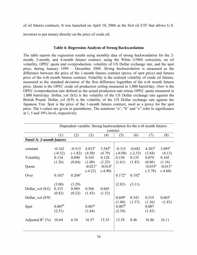
74

of oil futures contracts. It was launched on April 10, 2006 as the first oil ETF that allows U.S.

investors to put money directly on the price of crude oil.

Table 4: Regression Analysis of Strong Backwardation

The table reports the regression results using monthly data of strong backwardation for the 2-month, 3-month, and 4-month futures contract, using the White (1980) correction, on oil volatility, OPEC quota and overproduction, volatility of US Dollar exchange rate, and the spot price, during January 1999 – December 2008. Strong backwardation is measured as the difference between the price of the 1-month futures contract (proxy of spot price) and futures price of the n-th month futures contract. Volatility is the realized volatility of crude oil futures, measured as the standard deviation of the first difference logarithm of the n-th month futures price. Quota is the OPEC crude oil production ceiling measured in 1,000 barrel/day. Over is the OPEC overproduction rate defined as the actual production rate minus OPEC quota measured in 1,000 barrel/day. Dollar_vol ($/£) is the volatility of the US Dollar exchange rate against the British Pound. Dollar_vol ($/¥) is the volatility of the US Dollar exchange rate against the Japanese Yen. Spot is the price of the 1-month futures contract, used as a proxy for the spot price. The t-values are given in parentheses. The notations ―a‖, ―b‖ and ―c‖ refer to significance

at 1, 5 and 10% level, respectively.

Dependent variable: Strong backwardation for the n-th month futures contract

(1) (2) (3) (4) (5) (6) (7) (8) Panel A: 2-month futures constant -0.162 -0.515 4.833a 3.545a -0.315 -0.682 4.283a 3.095a (-0.52) (-1.82) (4.50) (4.79) (-0.98) (-2.33) (3.84) (4.13) Volatility 0.134 0.090 0.103 0.128 0.150 0.135 0.079 0.105 (1.26) (0.84) (1.00) (1.25) (1.61) (1.43) (0.86) (1.16) Quota -0.021a -0.014a -0.019a -0.013a (-4.22) (-4.90) (-3.78) (-4.60) Over 0.183a 0.204a 0.172a 0.192a

(3.00) (3.29) (2.82) (3.11)

Dollar_vol ($/£) 0.335 0.089 0.566 0.605 (0.82) (0.22) (1.43) (1.52) Dollar_vol ($/¥) 0.609c 0.543 0.519 0.603c (1.80) (1.57) (1.56) (1.83) Spot 0.007b 0.007c 0.007b 0.007 (2.51) (1.64) (2.54) (1.43) Adjusted R2 (%) 10.64 6.54 16.57 15.35 12.58 8.46 16.86 16.11

75

Table 4 continued (1) (2) (3) (4) (5) (6) (7) (8) Panel B: 3-month futures constant -0.068 -0.674 8.714a 6.512a -0.362 -0.995b 7.717a 5.727a (-0.13) (-1.4) (4.71) (5.17) (-0.67) (-1.99) (4.02) (4.47) Volatility 0.322c 0.261 0.255 0.294 0.362b 0.358b 0.223 0.265 (1.64) (1.31) (1.34) (1.54) (2.16) (2.08) (1.33) (1.60) Quota -0.036a -0.025a -0.033a -0.023a (-4.28) (-5.06 ) (-3.84) (-4.76) Over 0.335a 0.3720 0.314a 0.350a (3.19) (3.49) (3.01) (3.30) Dollar_vol ($/£) 0.551 0.149 0.933 0.992 (0.76) (0.21) (1.33) (1.41) Dollar_vol ($/¥) 1.125b 1.038c 0.959c 1.094b (1.93) (1.74) (1.67) (1.93) Spot 0.012a 0.012c 0.012a 0.011 (2.64) (1.62) (2.68) (1.39) Adjusted R2 (%) 12.86 8.37 18.19 17.05 15.17 10.66 18.9 18.25 Panel C: 4-month futures constant 0.086 -0.703 11.804a 8.934a -0.331 -1.171c 10.516a 7.952a (0.13) (-1.11) (4.76) (5.33) (-0.47) (-1.78) (4.09) (4.64) Volatility 0.466 0.412 0.345 0.390 0.545b 0.561b 0.337 0.387c (1.78) (1.54) (1.36) (1.53) (2.44) (2.44) (1.50) (1.74) Quota -0.048a -0.034a -0.044a -0.031a (-4.24) (-5.08) (-3.83) (-4.82) Over 0.467a 0.517a 0.438a 0.488a (3.34) (3.63) (3.15) (3.45) Dollar_vol ($/£) 0.583 0.100 1.033 1.096 (0.61) (0.10) (1.10) (1.16) Dollar_vol ($/¥) 1.498b 1.409c 1.258c 1.427c (1.93) (1.77) (1.63) (1.87) Spot 0.017a 0.016 0.016a 0.014 (2.69) (1.56) (2.73) (1.33) Adjusted R2 (%) 14.24 9.64 18.68 17.66 16.66 12.01 19.68 19.15

76

Table 5: Role of Oil Fund on Backwardation--Regression Analysis

The table reports the regression results using monthly data of weak and strong backwardation for the 2-month, 3-month, and 4-month futures contract, using the White (1980) correction, on oil volatility, OPEC quota and overproduction, volatility of US Dollar exchange rate, and the spot price, during April 2006 – December 2008. Weak backwardation is measured as the difference between the price of the 1-month futures contract (proxy of spot price) and discounted futures price of the n-th month futures contract. Strong backwardation is measured as the difference between the price of the 1-month futures contract and futures price of the n-th month futures contract. Volatility is the realized volatility of crude oil futures, measured as the standard deviation of the first difference logarithm of the n-th month futures price. Quota is the OPEC crude oil production ceiling measured in 1,000 barrel/day. Over is the OPEC overproduction rate defined as the actual production rate minus OPEC quota measured in 1,000 barrel/day. Dollar_vol ($/£) is the volatility of the US Dollar exchange rate against the British Pound. Dollar_vol ($/¥) is the volatility of the US Dollar exchange rate against the Japanese Yen. Spot is the price of the 1-month futures contract, used as a proxy for the spot price. Fund_volume is the natural logarithm of the United States oil fund trading volume. The t-values are given in parentheses. The notations ―a‖, ―b‖ and ―c‖ refer to significance at 1, 5 and 10% level, respectively.

Dependent variable: Weak backwardation

Dependent variable: Strong backwardation

(1) (2) (3) (4) (5) (6) (7) (8) Panel A: 2-month futures constant -4.171a 5.932c -3.965a 5.927c -4.924a 4.724 -4.694a 4.571 (-6.11) (1.70) (-6.01) (1.89) (-7.01) (1.30) (-7.01) (1.43) Volatility -0.291 -0.361 -0.211 -0.285 -0.325 -0.393 -0.271) -0.338 (-1.08) (-1.26) (-1.05) (-1.35) (-1.17) (-1.32) (-1.33) (-1.56) Quota -0.038b -0.038a -0.036b -0.035b (-2.66) (-2.89) (-2.43) (-2.63) Over 0.334a 0.310a 0.333a 0.302a (3.39) (3.30) (3.29) (3.17) Dollar_vol ($/£) 0.375 0.599 0.595 0.797 (0.60) (0.88) (0.92) 1.13) Dollar_vol ($/¥) 0.769c 1.026b 0.942b 1.189b (1.77) (2.30) (2.14) (2.60) Spot 0.038a 0.054a 0.034a 0.049a 0.039a 0.054a 0.035a 0.048a (6.41) (6.16) (5.61) ( 5.79) (6.38) (5.95) (5.59) (5.57) Fund _volume -0.015a -0.015a -0.014a -0.013a -0.014a -0.014a -0.013a -0.013a (-3.87) (-3.60) (-3.79) (-3.58) (-3.57) (-3.28) (-3.52) (-3.29) Adjusted R2 (%) 64.67 60.1 67.94 65.66 62.45 56.86 66.9 63.86

77

Table 5 continued

(1) (2) (3) (4) (5) (6) (7) (8) Panel B: 3-month futures constant -7.227a 11.050c -6.835a 11.227b -8.378a 9.325 -7.942a 9.292c (-6.49) (1.84) (-6.42) (2.11) (-7.29) (1.50) (-7.34) (1.71) Volatility -0.485 -0.608 -0.267 -0.398 -0.538 -0.660 -0.360 -0.480 (-1.04) (-1.21) (-0.79) (-1.11) (-1.12) (-1.27) (-1.05) (-1.30) Quota -0.069b -0.068a -0.067b -0.065a (-2.78) (-3.10) (-2.58) (-2.88) Over 0.611a 0.568a 0.614a 0.560a (3.65) (3.60) (3.55) (3.49) Dollar_vol ($/£) 0.511 0.911 0.840 1.211 (0.47) (0.76) (0.75) (0.97) Dollar_vol ($/¥) 1.439c 1.910b 1.701b 2.159b (1.96) (2.50) (2.28) 2.76) Spot 0.066a 0.094a 0.058a 0.084a 0.067a 0.094a 0.059a 0.083a (6.74) (6.32) (5.86) (6.02) (6.68) (6.12) (5.83) (5.81) Fund _volume -0.025a -0.025a -0.022a -0.022a -0.024a -0.023a -0.021a -0.021a (-3.93) (-3.58) (-3.78) (-3.52) (-3.64) (-3.28) (-3.54) (-3.25) Adjusted R2 (%) 66.44 61.05 70.37 67.69 64.19 57.83 69.34 65.94 Panel C: 4-month futures constant

-9.357a 15.344c -8.851a 15.618b -

10.915a 13.140 -10.341a 13.141c (-6.49) (1.91) (-6.43) (2.20) (-7.31) (1.57) (-7.38) (1.80) Volatility -0.563 -0.725 -0.233 -0.406 -0.636 -0.797 -0.359 -0.518 (-0.90) (-1.07) (-0.52) (-0.84) (-0.99) (-1.13) (-0.78) (-1.04) Quota -0.093a -0.093a -0.090b -0.088a (-2.80) (-3.14) (-2.60) (-2.92) Over 0.833a 0.775a 0.841a 0.768a (3.74) (3.70) (3.65) (3.60) Dollar_vol ($/£) 0.597 1.138 1.037 1.543 (0.41) (0.71) (0.69) (0.92) Dollar_vol ($/¥) 1.947c 2.589b 2.299b 2.928b (1.99) (2.53) (2.31) (2.78) Spot 0.086a 0.124a 0.077a 0.111a 0.089a 0.125a 0.077a 0.111a 6.86) (6.32) (5.96) (6.05) (6.79) (6.11) (5.91) (5.84) Fund _volume -0.032a -0.032a -0.029a -0.028a -0.031a -0.030a -0.027a -0.026a (-3.89) (-3.50) (-3.71) (-3.41) (-3.59) (-3.20) (-3.45) (-3.13) Adjusted R2 (%) 67.28 61.47 71.29 68.29 64.72 57.88 70.01 66.25

78

The regression analysis of weak and strong backwardation is repeated with the addition

of the monthly logarithm trading volume of USO. The regression is estimated using monthly

data between April 2006 and December 2008, which results in 33 monthly observations. The

results are reported in Table 5. As shown from the table, the USO volume coefficients are highly

significantly negative in all specifications. That is to say, the investment activities of USO fund

play an important role in driving up the futures prices in relative to the spot price (i.e., lowering

the level of backwardation). The regression results are also supported by Figure 5 which shows

the negative association between fund activities and the level of backwardation over time.

Moreover, it should be noted that the adjusted R2 improved substantially, when taking into

account the fund activities variable, compared with the value of adjusted R2 in Tables 3 and 4.

Nevertheless, the sample period is much shorter and the number of observations is smaller than

the earlier analysis, so caution must be taken in generalizing this sub-period analysis.

As for the other variables in the regression, the coefficients of OPEC qutoa and OPEC

overproduction variables stay significant; the oil spot coefficients are positively significant that

supports a binding production capacity constraint, and the coefficients of the volatility of the US

Dollar exchange rate against the Japanese Yen are positively significant as in Table 3 and 4.

79

Figure 5: Crude Oil Weak Backwardation and the United States Oil Fund (USO) Trading

Volume

(April 2006 – December 2008)

The figures 5-A and 5-B show the daily strong and weak backwardation of the 4-month futures contract respectively vs. the daily trading volume for the United States Oil Fund (symbol: USO). Strong backwardation is measured as the difference between the price of the 1-month futures contract (proxy of spot price) and futures price of the n-th month futures contract. Weak Backwardation is measured as the difference between the price of the 1-month futures contract and discounted futures price of the 4-month futures contract.

(A) USO trading volume and strong backwardation of the 4-month WTI futures contract.

(B) USO trading volume and weak backwardation of the 4-month WTI futures contract.

-15

-10

-5

0

5

10

15

0

10000

20000

30000

40000

50000

60000

Jul 06 Jan 07 Jul 07 Jan 08 Jul 08

Strong Backwardation

USO Volume

$1,0

00 S

hare

s

-15

-10

-5

0

5

10

15

0

10000

20000

30000

40000

50000

60000

Jul 06 Jan 07 Jul 07 Jan 08 Jul 08

USO Volume

$1

,000

Share

s

Weak Backwardation

80

5. Conclusion

This study shows that oil futures generally exhibit backwardation. Specificly, it shows

that oil futures are strongly and weakly backwardated 57% and 69% of the time, respectively,

during the period from January 1986 to December 2008. The study also finds that the level of

backwardation is higher for the far-month-futures contracts than that of the nearby futures

contracts.

This study further examines the influence of oil price volatility, the behavior of the

Organization of Petroleum Exporting Countries (OPEC), and the volatility of US Dollar

exchange rate on the extent of weak and strong backwardation of crude oil futures during

January 1986 – December 2008. The study builds on Litzenberger and Rabinowitz (1995)

theory that offer an explanation for the backwardation in oil futures based on the option pricing

theory.

Both Dollar value and OPEC behavior are believed to be important factors affecting oil

price. The regression results show that OPEC behavior significantly affect the relation between

spot and futures prices of oil. More specifically, the study finds that OPEC production quota

imposed on its members has a negative significant effect on weak and strong backwardation,

while the OPEC member’s overproduction (difference between quota and the actual production)

has a positive significant effect on oil backwardation. Put differently, the increased uncertainty

about the future supply of OPEC members due to the deviation from the allocated production

ceiling results in a greater backwardation level.

On the other hand, the uncertainty of US Dollar exchange rate is believed to discourage

current oil production; hence greater backwardations will be needed to encourage current

81

production. The weak and strong backwardation regression results show that the coefficients of

the volatility of US Dollar exchange rate against the Japanese Yen are positively significant.

However the volatility of US Dollar exchange rate against the British Pound has no significant

effect on oil backwardation. This difference in results could be explained by the fact that Japan

has been among the top three oil import countries, thus the dollar/yen exchange rate reflects

better than the dollar/pound rate the dollar revenue to oil surplus countries.

The regression analysis shows positive association between weak backwardation and

volatility in most specifications. This result confirms the prior work by Litzenberger and

Rabinowitz (1995). However, volatility is not significant in the strong backwardation regression.

The study also investigates the role of oil funds on the backwardation. To this regard, the

study includes the volume of the United States Oil fund (USO) in the regression analysis. The

results indicate a negative association between USO volume and backwardation. This result

makes sense since oil funds create demand on oil futures causing futures price to go up, thus

lower level of backwardation.

82

References

Adelman, Morris and G. Watkins. 2005. U.S. Oil and Natural Gas Reserve Prices, 1982-2003. Energy Economics 27(4), 553-571. Adelman, Morris. 1991. User Cost in Oil Production. Resources and Energy 13(3), 217-240. Alquist, Ron and Lutz Kilian. 2010. What Do We Learn from the Price of Crude Oil Futures? Journal of Applied Econometrics 25(4), 539-573.

Andreou, Elena and Eric Ghysels. 2002. Rolling-Sample Volatility Estimators: Some New Theoretical, Simulation, and Empirical Results. Journal of Business and Economic Statistics 20(3), 363-376

Black, Fischer. 1976. The Pricing of Commodity Contracts. Journal of Financial Economics 3(1-2), 167-179. Bollerslev, Tim. 1986. Generalized Autoregressive Conditional Heteroskedasticity. Journal of

Econometrics 31(3), 307-327. Brennan, Michael and Eduardo Schwartz. 1985. Evaluating Natural Resource Investments. Journal of Business 58(2), 135-157. Cairns, Robert and Graham Davis. 2001. Adelman’s Rule and the Petroleum Firm. The Energy

Journal 22(3), 31– 54. Carlson, Murray, Zeigham Khokher, and Sheridan Titman. 2007. Equilibrium Exhaustible Resource Price Dynamics. Journal of Finance 62(4), 1663-1703. Considine, Timothy and Donald Larson. 2001. Uncertainty and the Convenience Yield in Crude Oil Price Backwardations. Energy Economics 23(5), 533-548. Fama, Eugene and Kenneth French. 1987. Commodity Futures Prices: Some Evidence on Forecast Power, Premiums, and the Theory of Storage. Journal of Business 60(1), 55-73. Fama, Eugene and Kenneth French. 1988. Business Cycles and the Behavior of Metals Prices. Journal of Finance 43(3), 1075-1093. Fattouh, Bassam. 2007. The Drivers of Oil Prices: The Usefulness and Limitations of Non-Structural Model, the Demand–Supply Framework and Informal Approaches. Oxford Institute

for Energy Studies Working Paper 32. Foster, Dean and Daniel Nelson. 1996. Continuous Record Asymptotics for Rolling Sample Variance Estimators. Econometrica 64(1), 139-174.

83

Gibson, Rajna and Eduardo Schwartz. 1990. Stochastic Convenience Yields and the Pricing of Oil Contingent Claims. Journal of Finance 45(3), 959-976. Guidi, Francesco. 2009. Volatility and Long-Term Relations in Equity Markets: Empirical Evidence from Germany, Switzerland, and the UK. The IUP Journal of Financial Economics 7(2), 7-39. Heal, Geoffrey and Michael Barrow. 1980. The Relationship between Interest Rate and Metal Price Movements. Review of Economic Studies 47(1), 161-181. Horan, Stephen, Jeffrey Peterson, and James Mahar. 2004. Implied Volatility of Oil Futures Options Surrounding OPEC Meetings. The Energy Journal 25(3), 103-126. Hotelling, Harold. 1931. The Economics of Exhaustible Resources. Journal of Political

Economy 39(2), 137-175. Kaldor, Nicholas. 1939. Speculation and Economic Stability. Review of Economic Studies 7(1), 1-27. Kaufmann, Robert, Stephane Dees, Pavlos Karadeloglou, and Marcelo Sánchez. 2004. Does OPEC Matter? An Econometric Analysis of Oil Prices. The Energy Journal 25(4), 67-90. Knetsch, Thomas. 2007. Forecasting the Price of Crude Oil via Convenience Yield Predictions. Journal of Forecasting 26(7), 527-549. Larson, Donald. 1994. Copper and the Negative Price of Storage. Unpublished working paper, The World Bank. Litzenberger, Robert and Nir Rabinowitz. 1995. Backwardation in Oil Futures Markets: Theory and Empirical Evidence. Journal of Finance 50(5), 1517−1545. Martens, Martin and Jason Zein. 2004. Predicting Financial Volatility: High-Frequency Time Series Forecasts Vis-a-Vis Implied Volatility. Journal of Futures Markets 24(11), 1005-1028. Martin, Gael, Andrew Reidy, and Jill Wright. 2009. Dose the Option Market Produce Superior Forecasts of Noise-Corrected Volatility Measures? Journal of Applied Econometrics 24(1), 77-104. Milonas, Nikolaos and Thomas Henker. 2001. Price Spread and Convenience Yield Behavior in the International Oil Market. Applied Financial Economics 11(1), 23–36. Moebert, Jochen. 2007. Crude Oil Price Determinants. Unpublished paper, Technische Universität Darmstadt. Morse, Edward. 2006. The Global Oil Market Outlook: Ten Lessons about the Petroleum Sector. Presentation given at the 2006 Summer Fuels Outlook Conference Washington, D.C.

84

Neely, Christopher J. 2009. Forecasting Foreign Exchange Volatility: Why is Implied Volatility Biased and Inefficient? And Does It Matter? Journal of International Financial Markets,

Institutions and Money 19(1), 188-205. Smith, Kerry. 1981. The Empirical Relevance of Hotelling’s Model for Natural Resources.

Resources and Energy 3(2), 105-117. Thompson, Andrew. 2001. The Hotelling Principle, Backwardation of Futures Prices and the Values of Developed Petroleum Reserves–The Production Constraint Hypothesis. Resource and

Energy Economics 23(2), 133–156. Wang, Tao, Jingto Wu, and Jian Yang. 2008. Realized Volatility and Correlation in Energy Futures Markets. Journal of Futures Markets 28(10), 993–1011. White, Halbert. 1980. A Heteroskedastic-Consistent Covariance Matrix Estimator and a Direct Test for Heteroskedasticity. Econometrica 48(4), 817-28. Working, Holbrook. 1948. Theory of the Inverse Carrying Charge in Futures Markets. Journal of

Farm Economics 30(1), 1-28.

85

Appendix A

Regression Analysis of Weak Backwardation

The table reports the regression results using monthly data of weak backwardation for the 2-month, 3-month, and 4-month futures contract, using the White (1980) correction, on oil volatility, OPEC quota and overproduction, volatility of US Dollar exchange rate, and the spot price, during January 1999 – December 2008. Weak backwardation is measured as the difference between the price of the 1-month futures contract (proxy of spot price) and discounted futures price of the n-th month futures contract. Volatility is the unconditional variance of the n-th month oil futures using GARCH model. Quota is the OPEC crude oil production ceiling measured in 1,000 barrel/day. Over is the OPEC overproduction rate defined as the actual production rate minus OPEC quota measured in 1,000 barrel/day. Dollar_vol ($/£) is the volatility of the US Dollar exchange rate against the British Pound. Dollar_vol ($/¥) is the volatility of the US Dollar exchange rate against the Japanese Yen. Spot is the price of the 1-month futures contract, used as a proxy for the spot price. The t-values are given in parentheses. The notations ―a‖, ―b‖ and ―c‖ refer to significance at 1, 5 and 10% level, respectively.

Dependent variable: Weak backwardation for the n-th month futures contract (1) (2) (3) (4) (5) (6) (7) (8) Panel A: 2-month futures constant -0.196 -0.299 4.115a 2.381a -0.335 -0.451c 3.747a 2.057b (-0.73) (-1.22) (3.93) (3.41) (-1.19) (-1.81) (3.40) (2.81) Volatility 2.953b 2.879b 2.300c 2.726b 0.031a 0.031a 0.021c 0.026 (2.41) (2.35) (1.88) (2.23) (2.77) (2.79) (1.89) (2.31) Quota -0.017a -0.009a -1.600a -0.800a (-3.66) (-3.18) (-3.33) (-2.91) Over 0.176a 0.183a 0.167a 0.174a (3.05) (3.21) (2.90) (3.04) Dollar_vol ($/£) 0.214 0.152 0.380 0.420 (0.59) (0.43) (1.06) (1.16) Dollar_vol ($/¥) 0.435 0.421 0.380 0.482 (1.41) (1.37) (1.24) (1.57) Spot -0.002 0.010b -0.002 0.009b (-0.91) (2.20) (-0.89) (2.03) Adjusted R2 (%) 9.84 9.96 12.71 9.82 11.10 11.25 13.01 10.67 Panel B: 3-month futures constant -0.316 -0.487 7.974a 4.512a -0.627 -0.807c 7.266a 3.958a

(-0.66) (-1.14) (4.52) (3.70) (-1.28) (-1.88) (3.95) (3.09) Volatility 4.523b 4.766b 4.740b 4.164c 0.051a 0.054a 0.043b 0.041b (2.04) (2.17) (2.20) (1.89) (2.62) (2.84) (2.24) (2.12) Quota -0.034a -0.017a -3.100a -1.500a (-4.21) (-3.43) (-3.90) (-3.19) Over 0.322a 0.332a 0.305a 0.315a (3.22) (3.37) (3.06) (3.19)

86

Appendix A continued (1) (2) (3) (4) (5) (6) (7) (8) Dollar_vol ($/£) 0.179 0.143 0.719 0.579 (0.27) (0.22) (1.12) (0.88) Dollar_vol ($/¥) 0.742 0.748 0.703 0.814 (1.38) (1.39) (1.34) (1.52) Spot -0.004 0.019a -0.003 0.018b (-0.80) (2.66) (-0.77) (2.46) Adjusted R2 (%) 10.53 10.8 15.49 11.07 11.92 12.23 15.87 12.22 Panel C: 4-month futures constant 0.117 -0.206 11.170a 6.965a -0.426 -0.888 10.883a 6.634a (0.19) (-0.36) (4.62) (4.24) (-0.64) (-1.50) (4.34) (3.88) Volatility 0.044 -0.034 -0.080 0.074 0.001 0.000+ -0.001 0.001 (0.20) (-0.16) (-0.37) (0.36) (0.30) (0.14) (-0.33) (0.39) Quota -0.045a -0.024a -4.600a -2.500a (-4.07) (-3.66) (-4.12) (-3.86) Over .440a 0.462a 0.417a 0.443a (3.26) (3.45) (3.05) (3.25) Dollar_vol ($/£) -0.975 -1.137 -0.326 -0.356 (-1.32) (-1.57) (-0.45) (-0.48) Dollar_vol ($/¥) 0.283 0.218 0.300 0.473 (0.40) (0.31) (0.45) (0.69) Spot -0.007 0.024b -0.009 0.024b (-1.17) (2.33) (-1.45) (2.28) Adjusted R2 (%) 8.59 8.31 12.72 9.37 7.33 6.44 12.71 9.56

87

Appendix B

Correlation Matrix

Volatility is the unconditional variance of the n-th month oil futures using GARCH model. Quota is the OPEC crude oil production ceiling measured in 1,000 barrel/day. Over is the OPEC overproduction rate defined as the actual production rate minus OPEC quota measured in 1,000 barrel/day. Dollar_vol ($/£) is the volatility of the US Dollar exchange rate against the British Pound. Dollar_vol ($/¥) is the volatility of the US Dollar exchange rate against the Japanese Yen. Spot is the price of the 1-month futures contract, used as a proxy for the spot price. Fund_volume is the natural logarithm of the United States oil fund trading volume.

Volatility 2-month

Volatility 3-month

Volatility 4-month

Quota Over Dollar_vol ($/£)

Dollar_vol ($/¥)

Fund _volume

January 1999 – December 2008

Volatility 2-month 1.000 Volatility 3-month 0.994 1.000 Volatility 4-month 0.955 0.966 1.000 Quota -0.048 -0.093 -0.121 1.000 Over -0.067 -0.064 -0.079 -0.479 1.000 Dollar_vol ($/£) -0.570 -0.605 -0.609 0.227 0.063 1.000 Dollar_vol ($/¥) -0.397 -0.410 -0.414 -0.025 0.139 0.485 1.000

April 2006 – December 2008

Volatility 2-

month 1.000 Volatility 3-month 0.999 1.000 Volatility 4-month 0.998 1.000 1.000 Quota -0.177 -0.201 -0.217 1.000 Over

-0.109 -0.103 -0.099 -0.515 1.000 Dollar_vol ($/£) -0.855 -0.862 -0.865 0.252 0.027 1.000 Dollar_vol ($/¥) -0.593 -0.607 -0.616 0.361 0.126 0.823 1.000 Fund _volume -0.788 -0.791 -0.793 0.394 0.137 0.594 0.463 1.000

88

Vita

Iman Adeinat was born in Los Angeles, CA. She received her Bachelor of Industrial Engineering

from the University of Jordan in 2003. She worked for a year as an Industrial Engineer at Petra

Engineering Industries—Jordan. She received her master of Engineering Management in 2007

from the University of New Orleans (UNO). She is also a 2011 graduate of the doctoral program

in Engineering and Applied Science—Engineering Management at the UNO. While at UNO, she

worked as graduate assistant at Center for Hazards Assessment, Response & Technology

(CHART). She received the Shell Exploration and Production - Outstanding Ph.D. Student

Award.