"First class futures"
201
UNIVERSITÉ DE NICE - SOPHIA ANTIPOLIS École Doctorale STIC Sciences et Technologies de l’Information et de la Communication THÈSE pour obtenir le titre de Docteur en Sciences de l’Université de Nice - Sophia Antipolis Mention Informatique présentée et soutenue par Muhammad Khurram BHATTI Energy-aware Scheduling for Multiprocessor Real-time Systems Thèse dirigée par Cécile BELLEUDY Laboratoire LEAT, Université de Nice-Sophia Antipolis -CNRS, Sophia Antipolis soutenue le 18 avril 2011, devant le jury composé de: Président du Jury Lionel Torres Pr. Université de Montpellier-II, France Rapporteurs Isabelle Puaut Pr. Université de Rennes-I, France Guy Gogniat Pr. Université de Bretagne Sud, France Examinateurs Yvon Trinquet Pr. Université de Nantes, France Lionel Torres Pr. Université de Montpellier-II, France Michel Auguin DR. CNRS, France (Co-directeur de thèse) Directeur de thèse Cécile Belleudy Maître de Conférences, Université de Nice-Sophia Antipolis, France
-
Upload
khangminh22 -
Category
Documents
-
view
0 -
download
0
Transcript of "First class futures"

UNIVERSITÉ DE NICE - SOPHIA ANTIPOLIS
École Doctorale STIC
Sciences et Technologies de l’Information et de la Communication
THÈSE
pour obtenir le titre de
Docteur en Sciences
de l’Université de Nice - Sophia Antipolis
Mention Informatique
présentée et soutenue par
Muhammad Khurram BHATTI
Energy-aware Scheduling forMultiprocessor Real-time Systems
Thèse dirigée par Cécile BELLEUDY
Laboratoire LEAT, Université de Nice-Sophia Antipolis -CNRS, Sophia Antipolis
soutenue le 18 avril 2011, devant le jury composé de:
Président du Jury Lionel Torres Pr. Université de Montpellier-II, France
Rapporteurs Isabelle Puaut Pr. Université de Rennes-I, France
Guy Gogniat Pr. Université de Bretagne Sud, France
Examinateurs Yvon Trinquet Pr. Université de Nantes, France
Lionel Torres Pr. Université de Montpellier-II, France
Michel Auguin DR. CNRS, France (Co-directeur de thèse)
Directeur de thèse Cécile Belleudy Maître de Conférences,Université de Nice-Sophia Antipolis, France


c© 2011Muhammad Khurram BhattiALL RIGHTS RESERVED

iii
AbstractReal-time applications have become more sophisticated and complex in their
behavior and interaction over the time. Contemporaneously, multiprocessor archi-tectures have emerged to handle these sophisticated applications. Inevitably, thesecomplex real-time systems, encompassing a range from small-scale embedded devicesto large-scale data centers, are increasingly challenged to reduce energy consump-tion while maintaining assurance that timing constraints will be met. To addressthis issue in real-time systems, many software-based approaches such as dynamicvoltage and frequency scaling and dynamic power management have emerged. Yettheir flexibility is often matched by the complexity of the solution, with the ac-companying risk that deadlines will occasionally be missed. As the computationaldemands of real-time embedded systems continue to grow, effective yet transpar-ent energy-management approaches will become increasingly important to minimizeenergy consumption, extend battery life, and reduce thermal losses. We believethat power- and energy-efficiency and scheduling of real-time systems are closely re-lated problems, which should be tackled together for best results. By exploiting thecharacteristic parameters of real-time application tasks, the energy-consciousness ofscheduling algorithms and the quality of service of real-time applications can besignificantly improved.
To support our thesis, this dissertation proposes novel approaches for energy-management within the paradigm of energy-aware scheduling for soft and hard real-time applications, which are scheduled over identical multiprocessor platforms. Ourfirst contribution is a Two-level Hierarchical Scheduling Algorithm (2L-HiSA) formultiprocessor systems, which falls in the category of restricted-migration schedul-ing. 2L-HiSA addresses the sub-optimality of EDF scheduling algorithm in mul-tiprocessors by dividing the problem into a two-level hierarchy of schedulers. Oursecond contribution is a dynamic power management technique, called the AssertiveDynamic Power Management (AsDPM) technique. AsDPM serves as an admissioncontrol technique for real-time tasks, which decides when exactly a ready task shallexecute, thereby reducing the number of active processors, which eventually reducesenergy consumption. Our third contribution is a dynamic voltage and frequencyscaling technique, called the Deterministic Stretch-to-Fit (DSF) technique, whichfalls in the category of inter-task DVFS techniques and works in conjunction withglobal scheduling algorithms. DSF comprises an online Dynamic Slack Reclama-tion algorithm (DSR), an Online Speculative speed adjustment Mechanism (OSM),and an m-Task Extension (m-TE) technique. Our fourth and final contribution isa generic power/energy management scheme for multiprocessor systems, called theHybrid Power Management (HyPowMan) scheme. HyPowMan serves as a top-levelentity that, instead of designing new power/energy management policies (whetherDPM or DVFS) for specific operating conditions, takes a set of well-known exist-ing policies. Each policy in the selected policy set performs well for a given set ofoperating conditions. At runtime, the best-performing policy for given workload isadapted by the HyPowMan scheme through a machine-learning algorithm.


v
To my father Ismail, who always dared to dream,and to my mother Mumtaz (late) for making it a reality.

vii
AcknowledgmentsCompletion of my PhD required countless selfless acts of support, generosity,
and time by people in my personal and academic life. I can only attempt to humblyacknowledge and thank the people and institutions that have given so freely through-out my PhD career and made this dissertation possible. I am thankful to the HigherEducation Commission (HEC) of Pakistan for providing uninterrupted funding sup-port throughout my Masters and PhD career. I am sincerely thankful to CécileBelleudy, my advisor, for being a constant source of invaluable encouragement, aid,and expertise during my years at University of Nice. While many students are for-tunate to find a single mentor, I have been blessed with two. I am deeply gratefulto Michel Auguin, my co-advisor, for the guidance, support, respect, and kindnessthat he has shown me over the last four years. The mentoring, friendship, and colle-giality of both Cécile and Michel enriched my academic life and have left a profoundimpression on how academic research and collaboration should ideally be conducted.
I am extremely thankful to the members of my dissertation committee. GuyGogniat and Isabelle Puaut have graciously accepted to serve on the committeeas reviewers and provided unique feedback, comments, and questions on multipro-cessor scheduling, along with a lot of encouragement. Yvon Trinquet has providedme with wise advice and support throughout my PhD and also accepted to be apart of my dissertation committee. I have always admired his precise questions andunique manner of addressing difficult research problems. Lionel Torres has beenvery kind for accepting to be the president of dissertation committee and a sourceof insightful comments and ideas to my research and its effective presentation. Imust acknowledge that all these people have greatly inspired me. Other colleagueswho I owe gratitude for their support of my research or major PhD milestones in-clude: Sébastian Bilavarn, Francois Verdier, Ons Mbarek, and Jabran Khan. I amalso grateful to the always helpful LEAT research laboratory and University of Nicestaff. I would like to thank all my research collaborators who have enhanced my en-thusiasm and understanding of real-time systems through various projects, namely;the collaborators of Pherma, COMCAS, and STORM tool design and developmentprojects. Since the path through the PhD program would be much more difficultwithout examples of success, I am indebted to Muhammad Farooq who has givenfriendship and guidance as recent real-time system PhD graduate from LEAT.
My family and friends have been an unending source of love and inspirationthroughout my PhD career. My father, Ismail, has offered unconditional under-standing and encouragement. My sisters, Shaista and Sofia, have kept me sane withtheir humor and understanding even from distance. My brother, Asad, has been agreat and selfless support to me throughout these year of my absence from home.My friends in French Riviera, Najam, Naveed, Uzair, Sabir, Chafic, Umer, Siouar,Khawla, Amel, Alice, and Sébastian have provided hours of enjoyable distractionfrom my work. I will always remember the time I have shared with them. Lastly,I can only wish if my mother, Mumtaz, was still alive to embrace me on achievingthis milestone. She will always remain my constant.

Contents
I Complete dissertation: English version 1
1 Introduction 31.1 Introduction . . . . . . . . . . . . . . . . . . . . . . . . . . . . . . . . 31.2 Contributions . . . . . . . . . . . . . . . . . . . . . . . . . . . . . . . 51.3 Summary . . . . . . . . . . . . . . . . . . . . . . . . . . . . . . . . . 8
2 Background on Real-time and Energy-efficient Systems 112.1 Real-time Systems . . . . . . . . . . . . . . . . . . . . . . . . . . . . 11
2.1.1 Real-time Workload . . . . . . . . . . . . . . . . . . . . . . . 122.1.2 Processing Platform . . . . . . . . . . . . . . . . . . . . . . . 162.1.3 Real-time Scheduling . . . . . . . . . . . . . . . . . . . . . . . 172.1.4 Real-time Scheduling in Multiprocessor Systems . . . . . . . . 20
2.2 Power- and Energy-efficiency in Real-time Systems . . . . . . . . . . 232.2.1 Power and Energy Model . . . . . . . . . . . . . . . . . . . . 232.2.2 Energy-aware Real-time Scheduling . . . . . . . . . . . . . . . 26
2.3 Simulation Environment . . . . . . . . . . . . . . . . . . . . . . . . . 282.4 Summary . . . . . . . . . . . . . . . . . . . . . . . . . . . . . . . . . 29
3 Two-level Hierarchical Scheduling Algorithm for MultiprocessorSystems 313.1 Introduction . . . . . . . . . . . . . . . . . . . . . . . . . . . . . . . . 313.2 Related Work . . . . . . . . . . . . . . . . . . . . . . . . . . . . . . . 323.3 Two-level Hierarchical Scheduling Algorithm . . . . . . . . . . . . . . 35
3.3.1 Basic Concept . . . . . . . . . . . . . . . . . . . . . . . . . . . 363.3.2 Working Principle . . . . . . . . . . . . . . . . . . . . . . . . 373.3.3 Runtime View of Schedule from Different Levels of Hierarchy 413.3.4 Schedulability Analysis . . . . . . . . . . . . . . . . . . . . . . 44
3.4 Experiments . . . . . . . . . . . . . . . . . . . . . . . . . . . . . . . . 473.4.1 Setup . . . . . . . . . . . . . . . . . . . . . . . . . . . . . . . 473.4.2 Functional Evaluation . . . . . . . . . . . . . . . . . . . . . . 473.4.3 Energy-efficiency of 2L-HiSA . . . . . . . . . . . . . . . . . . 503.4.4 Performance Evaluation . . . . . . . . . . . . . . . . . . . . . 52
3.5 Concluding Remarks . . . . . . . . . . . . . . . . . . . . . . . . . . . 55
4 Assertive Dynamic Power Management Technique 574.1 Dynamic Power Management . . . . . . . . . . . . . . . . . . . . . . 574.2 Related Work . . . . . . . . . . . . . . . . . . . . . . . . . . . . . . . 584.3 Assertive Dynamic Power Management Technique . . . . . . . . . . . 61
4.3.1 Laxity Bottom Test (LBT) . . . . . . . . . . . . . . . . . . . 624.3.2 Working Principle . . . . . . . . . . . . . . . . . . . . . . . . 64
x Contents
4.3.3 Choice of Power-efficient State . . . . . . . . . . . . . . . . . 684.4 Static Optimizations using AsDPM . . . . . . . . . . . . . . . . . . . 694.5 Experiments . . . . . . . . . . . . . . . . . . . . . . . . . . . . . . . . 69
4.5.1 Target Application . . . . . . . . . . . . . . . . . . . . . . . . 694.5.2 Simulation Results . . . . . . . . . . . . . . . . . . . . . . . . 734.5.3 Comparative Analysis of the AsDPM Technique . . . . . . . . 78
4.6 Future Perspectives of the AsDPM Technique . . . . . . . . . . . . . 794.6.1 Memory Subsystem . . . . . . . . . . . . . . . . . . . . . . . . 804.6.2 Thermal Load Balancing . . . . . . . . . . . . . . . . . . . . . 82
4.7 Concluding Remarks . . . . . . . . . . . . . . . . . . . . . . . . . . . 84
5 Deterministic Stretch-to-Fit DVFS Technique 855.1 Dynamic Voltage and Frequency Scaling . . . . . . . . . . . . . . . . 855.2 Related Work . . . . . . . . . . . . . . . . . . . . . . . . . . . . . . . 875.3 Deterministic Stretch-to-Fit Technique . . . . . . . . . . . . . . . . . 90
5.3.1 Dynamic Slack Reclamation (DSR) Algorithm . . . . . . . . . 905.3.2 Online Canonical Schedule . . . . . . . . . . . . . . . . . . . . 935.3.3 Online Speculative speed adjustment Mechanism (OSM) . . . 975.3.4 m-Tasks Extension Technique (m-TE) . . . . . . . . . . . . . 98
5.4 Experiments . . . . . . . . . . . . . . . . . . . . . . . . . . . . . . . . 985.4.1 Setup . . . . . . . . . . . . . . . . . . . . . . . . . . . . . . . 995.4.2 Target Application . . . . . . . . . . . . . . . . . . . . . . . . 995.4.3 Simulation Results . . . . . . . . . . . . . . . . . . . . . . . . 99
5.5 Concluding Remarks . . . . . . . . . . . . . . . . . . . . . . . . . . . 104
6 Hybrid Power Management Scheme for Multiprocessor Systems 1076.1 Introduction . . . . . . . . . . . . . . . . . . . . . . . . . . . . . . . . 1076.2 Related Work . . . . . . . . . . . . . . . . . . . . . . . . . . . . . . . 1086.3 Hybrid Power Management Scheme . . . . . . . . . . . . . . . . . . . 109
6.3.1 Machine-learning Algorithm . . . . . . . . . . . . . . . . . . . 1106.3.2 Selection of Experts . . . . . . . . . . . . . . . . . . . . . . . 114
6.4 Experiments . . . . . . . . . . . . . . . . . . . . . . . . . . . . . . . . 1146.4.1 Setup . . . . . . . . . . . . . . . . . . . . . . . . . . . . . . . 1146.4.2 Description of Experts . . . . . . . . . . . . . . . . . . . . . . 1156.4.3 Simulation Results . . . . . . . . . . . . . . . . . . . . . . . . 116
6.5 Concluding Remarks . . . . . . . . . . . . . . . . . . . . . . . . . . . 120
7 Conclusions and Future Research Perspectives 1237.1 Summary of Contributions and Results . . . . . . . . . . . . . . . . . 1247.2 Future Research Perspectives . . . . . . . . . . . . . . . . . . . . . . 127
7.2.1 Task Models . . . . . . . . . . . . . . . . . . . . . . . . . . . 1277.2.2 Platform Architectures . . . . . . . . . . . . . . . . . . . . . . 1287.2.3 Scheduling Algorithms . . . . . . . . . . . . . . . . . . . . . . 1287.2.4 Implementation strategy –Simulations vs Real Platforms . . . 129
Contents xi
7.2.5 Thermal Aspects . . . . . . . . . . . . . . . . . . . . . . . . . 1307.3 Summary . . . . . . . . . . . . . . . . . . . . . . . . . . . . . . . . . 130
II Selected chapters: French version 133
1 Introduction 1351.1 Introduction . . . . . . . . . . . . . . . . . . . . . . . . . . . . . . . . 1351.2 Contributions . . . . . . . . . . . . . . . . . . . . . . . . . . . . . . . 1371.3 Résumé . . . . . . . . . . . . . . . . . . . . . . . . . . . . . . . . . . 140
2 Conclusions et Perspectives 1432.1 Résumé des Contributions et Résultats . . . . . . . . . . . . . . . . . 1442.2 Perspectives . . . . . . . . . . . . . . . . . . . . . . . . . . . . . . . . 147
2.2.1 Modèle des tâches . . . . . . . . . . . . . . . . . . . . . . . . 1472.2.2 Architectures de Plate-forme Cible . . . . . . . . . . . . . . . 1482.2.3 Les algorithmes d’ordonnancement . . . . . . . . . . . . . . . 1492.2.4 Stratégie d’implementation . . . . . . . . . . . . . . . . . . . 1502.2.5 Aspects Thermiques . . . . . . . . . . . . . . . . . . . . . . . 150
2.3 Résumé . . . . . . . . . . . . . . . . . . . . . . . . . . . . . . . . . . 151
A STORM: Simulation TOol for Real-time Multiprocessor Schedul-ing 155A.1 Functional Architecture . . . . . . . . . . . . . . . . . . . . . . . . . 156
A.1.1 Software Entities . . . . . . . . . . . . . . . . . . . . . . . . . 157A.1.2 Hardware Entities . . . . . . . . . . . . . . . . . . . . . . . . 158A.1.3 System Entities . . . . . . . . . . . . . . . . . . . . . . . . . . 159A.1.4 Simulation Kernel . . . . . . . . . . . . . . . . . . . . . . . . 159
B HyPowMan Scheme: Additional Simulation Results 161B.1 Simulation Results Using AsDPM & DSF Experts . . . . . . . . . . 161
B.1.1 Effect of variations in bcet/wcet ratio . . . . . . . . . . . . . 161B.1.2 Effect of variations in number of tasks . . . . . . . . . . . . . 161B.1.3 Effect of Variations in total utilization . . . . . . . . . . . . . 162
B.2 Simulation Results Using ccEDF & DSF Experts . . . . . . . . . . . 163
Bibliography 167

List of Algorithms
1 Offline task partitioning to processors . . . . . . . . . . . . . . . . . 382 Offline processor-grouping . . . . . . . . . . . . . . . . . . . . . . . . 393 Local-level scheduler: Online jobs assignment for partitioned tasks
present in τπk . . . . . . . . . . . . . . . . . . . . . . . . . . . . . . . 434 Top-level scheduler: Online jobs assignment for migrating tasks
present in τglob . . . . . . . . . . . . . . . . . . . . . . . . . . . . . . 435 Assertive Dynamic Power Management . . . . . . . . . . . . . . . 656 Dynamic Slack Reclamation . . . . . . . . . . . . . . . . . . . . . 917 Online Speculation Mechanism . . . . . . . . . . . . . . . . . . . . 988 m-Tasks Extension Technique . . . . . . . . . . . . . . . . . . . . 989 Machine-learning . . . . . . . . . . . . . . . . . . . . . . . . . . . . 113

List of Figures
2.1 Illustration of various characteristic parameters of real-time tasks.Periodic task Ti has an implicit deadline (di=Pi) with the followingvalues of other parameters. Oi=2, Ci=3, di=Pi=4, and Li=1. . . . . 15
2.2 High-level illustration of symmetric share-memory multiprocessor(SMP) architecture layout of processing platform. . . . . . . . . . . . 18
2.3 No migration scheduling. . . . . . . . . . . . . . . . . . . . . . . . . . 212.4 Full migration scheduling. . . . . . . . . . . . . . . . . . . . . . . . . 212.5 Restricted migration scheduling. . . . . . . . . . . . . . . . . . . . . 212.6 Current and future trends in the evolution of portable embedded
system demand, their power consumption, and their energy-densityin batteries. (a) Evolution of the demand for portable equipmentover the years (SEMICO Research Corp.). (b) Power consumptionin portable equipment over the years (ITRS 2008). (c) Evolution ofenergy-density in batteries over the years (EPoSS 2009). . . . . . . . 24
2.7 Example of energy management decision-making of DPM technique. 272.8 Example of energy management decision-making of DVFS technique. 27
3.1 Job-splitting of a migrating task over three processors. . . . . . . . . 333.2 Two-level hierarchical scheduling approach based on restricted migra-
tion. . . . . . . . . . . . . . . . . . . . . . . . . . . . . . . . . . . . . 363.3 Example schedule of partitioned tasks under EDF scheduling al-
gorithm on SMP architecture (n=6, m=4), illustrating the under-utilization of platform. . . . . . . . . . . . . . . . . . . . . . . . . . . 40
3.4 Illustration of T dk occurring on different processors with respect tothe proportionate under-utilization available on each processor. . . . 42
3.5 View of runtime schedule by top-level and local-level schedulers under2L-HiSA on an SMP architecture. . . . . . . . . . . . . . . . . . . . . 44
3.6 Simulation traces of partitioned tasks under EDF local scheduler oneach processor. . . . . . . . . . . . . . . . . . . . . . . . . . . . . . . 49
3.7 Simulation traces of partitioned tasks in the presence of T dk underEDF local scheduler on each processor. . . . . . . . . . . . . . . . . . 50
3.8 Simulation traces of migrating and partitioned tasks together underEDF local- and top-level schedulers. . . . . . . . . . . . . . . . . . . 51
3.9 Simulation traces of EDF global scheduling of task set τ on fourprocessors. . . . . . . . . . . . . . . . . . . . . . . . . . . . . . . . . . 52
3.10 Simulation traces of individual tasks under global EDF scheduler . . 533.11 Number of task preemptions under 2L-HiSA, PFair (PD2), and
ASEDZL algorithms. . . . . . . . . . . . . . . . . . . . . . . . . . . . 543.12 Number of task migrations under 2L-HiSA, PFair (PD2), and
ASEDZL algorithms. . . . . . . . . . . . . . . . . . . . . . . . . . . . 55

xvi List of Figures
4.1 Laxity Bottom Test (LBT) using anticipative laxity li. . . . . . . . . 644.2 Schedule of τ using global EDF scheduler. (a) Without AsDPM. (b)
With AsDPM. . . . . . . . . . . . . . . . . . . . . . . . . . . . . . . 654.3 Impact of an intermediate priority task’s release. (a) Projected sched-
ule of tasks at time tc without intermediate priority task T3. (b) Pro-jected schedule of tasks at time tc+1 with intermediate priority taskT3. . . . . . . . . . . . . . . . . . . . . . . . . . . . . . . . . . . . . . 68
4.4 Block diagram of H.264 video decoding scheme. . . . . . . . . . . . . 704.5 Block diagram of H.264 decoding scheme slices version. . . . . . . . . 714.6 Block diagram of H.264 decoding scheme pipeline version. . . . . . . 724.7 Simulation results on the changes in energy consumption for H.264
video decoder application (slices version) for various frequencies. . . 734.8 Simulation results on energy consumption under statically non-
optimized EDF schedule and statically optimized EDF schedule usingAsDPM for H.264 video decoder application (slices version). . . . . . 77
4.9 Simulation results on energy consumption under statically non-optimized EDF schedule and statically optimized EDF schedule usingAsDPM for H.264 video decoder application (pipeline version). . . . 78
4.10 Simulation results on the energy consumption under statically non-optimized EDF schedule, statically optimized EDF schedule usingAsDPM, and EDF schedule using online AsDPM for H.264 videodecoder application (slices version). . . . . . . . . . . . . . . . . . . . 79
4.11 Simulation results on the energy consumption under statically non-optimized EDF schedule, statically optimized EDF schedule usingAsDPM, and EDF schedule using online AsDPM for H.264 videodecoder application (pipeline version). . . . . . . . . . . . . . . . . . 80
4.12 Simulation results on energy consumption of AsDPM in comparisonwith ideal DPM technique under the control of EDF scheduling algo-rithm for H.264 video decoder application (slices version). . . . . . . 81
4.13 Energy consumption in memory subsystem using multi-bank archi-tecture. (a) Energy consumption of multi-bank memory under globalEDF schedule without AsDPM. (b) Energy consumption optimiza-tion of multi-bank memory under global EDF schedule using AsDPM. 83
5.1 Dynamic slack redistribution of a task under various DVFS strategies. 885.2 Slack reclamation using the DSR algorithm. . . . . . . . . . . . . . . 935.3 Simulation traces of example task set on a single processor. a) Canon-
ical schedule of tasks where all tasks execute with worst-case execu-tion time. b) Practical schedule of tasks where T1 finishes earlier thanits WCET and T1 exploits dynamic slack to elongate its WCET atruntime. . . . . . . . . . . . . . . . . . . . . . . . . . . . . . . . . . . 94
5.4 Task T2 consumes ε to elongate its execution up to its terminationinstant in canonical schedule. . . . . . . . . . . . . . . . . . . . . . . 95
5.5 Task queues managed by a global scheduler at runtime. . . . . . . . 95
List of Figures xvii
5.6 Construction of online canonical schedule ahead of practical schedulefor m-tasks. . . . . . . . . . . . . . . . . . . . . . . . . . . . . . . . . 96
5.7 Simulation results of H.264 slices version. . . . . . . . . . . . . . . . 1005.8 Simulation results of H.264 pipeline version. . . . . . . . . . . . . . . 1015.9 Simulation results of H.264 pipeline version illustrating the effective-
ness of OSM. . . . . . . . . . . . . . . . . . . . . . . . . . . . . . . . 1025.10 Comparative analysis of simulation results of H.264 slices version. . . 1035.11 Comparative analysis of simulation results of H.264 pipeline version. 104
6.1 Interplay of DPM and DVFS policies. . . . . . . . . . . . . . . . . . 1096.2 Arrangement of expert set under the HyPowMan scheme for an SMP
architecture. . . . . . . . . . . . . . . . . . . . . . . . . . . . . . . . . 1106.3 Example of the weight and probability update of a DPM-based expert.1126.4 Simulation results on variation of bcet/wcet ratio. . . . . . . . . . . . 1176.5 Simulation results on variation in number of tasks. . . . . . . . . . . 1186.6 Simulation results on variation in aggregate utilization. . . . . . . . . 1196.7 Simulation results on variation in α. . . . . . . . . . . . . . . . . . . 1206.8 Simulation results on variation in β. . . . . . . . . . . . . . . . . . . 121
A.1 STORM simulator input and output file system. . . . . . . . . . . . 156A.2 Functional architecture of STORM simulator. . . . . . . . . . . . . . 157A.3 STORM: various states for application tasks. . . . . . . . . . . . . . 157A.4 STORM: example XML file. . . . . . . . . . . . . . . . . . . . . . . . 158
B.1 Simulation results on variation of bcet/wcet ratio. . . . . . . . . . . . 162B.2 Simulation results on variation in number of tasks. . . . . . . . . . . 162B.3 Simulation results on variation in aggregate utilization. . . . . . . . . 163B.4 Simulation results on variation in bcet/wcet ratio. . . . . . . . . . . . 164B.5 Simulation results on the usage of experts under the HyPowMan scheme.164

List of Tables
2.1 Voltage-frequency levels of PXA270 processor . . . . . . . . . . . . . 292.2 Power-efficient states of PXA270 processor @ 624-MHz & 1.55-volts . 29
3.1 Real-time periodic task set τ . . . . . . . . . . . . . . . . . . . . . . 483.2 Parameters of dummy tasks (T dk ) on each processor . . . . . . . . . . 48
4.1 H.264 video decoder application task set for slices version . . . . . . 714.2 H.264 video decoder application task set for pipeline version . . . . . 724.3 Static architecture configurations for H.264 video decoder slices version 744.4 Static architecture configurations for H.264 video decoder pipeline
version . . . . . . . . . . . . . . . . . . . . . . . . . . . . . . . . . . . 754.5 Static optimal architecture configurations for H.264 video decoder
slices version for different QoS requirements . . . . . . . . . . . . . . 764.6 Static optimal architecture configurations for H.264 video decoder
pipeline version for different QoS requirements . . . . . . . . . . . . . 76
5.1 Simulation settings for H.264 video decoder slices version . . . . . . . 1005.2 Simulation settings for H.264 video decoder pipeline version . . . . . 101
6.1 Simulation settings for variable bcet/wcet ratio . . . . . . . . . . . . 1166.2 Simulation settings for variable number of tasks . . . . . . . . . . . . 1176.3 Simulation settings for variable aggregate utilization . . . . . . . . . 1186.4 Simulation settings for variable α . . . . . . . . . . . . . . . . . . . . 1196.5 Simulation settings for variable β . . . . . . . . . . . . . . . . . . . . 120
B.1 Simulation settings for variable bcet/wcet ratio . . . . . . . . . . . . 163

xx List of Tables
Symbols and Acronyms
Symbols Definition
t Time instantτ Task setTi Individual task indexed as iTi,j Individual job j of task TiJ Job setri Release time of task TiCi Worst-case execution time (WCET) of task Tidi Relative deadline of task TiPi Period of task TiOi Offset of first job Ti,1 of Ti w.r.t. system activationLi Absolute laxity of task Tili Anticipative laxity of task Tiui Utilization of individual task TiUsum(τ) Utilization of task set τπk Individual processor indexed as kΠ Processor set/ platformn Number of tasks in τm Number of processors in Π
ν Speed of processor πkFop Operating frequencyVop Operating voltageVth Threshold voltageE Energyε Dynamic slackφ Scaling factorPwr(ν) Power as function of speed ντπk Subset of tasks partitioned on processor πkScan Canonical Schedule of tasksSpra Practical Schedule of tasksDBF (τ, L) Demand Bound Function of task set τ over interval
of length LN Number of Experts (where, expert is any power
management scheme)w Weight factor for individual expertW Weight vector for expert set
continued on next page
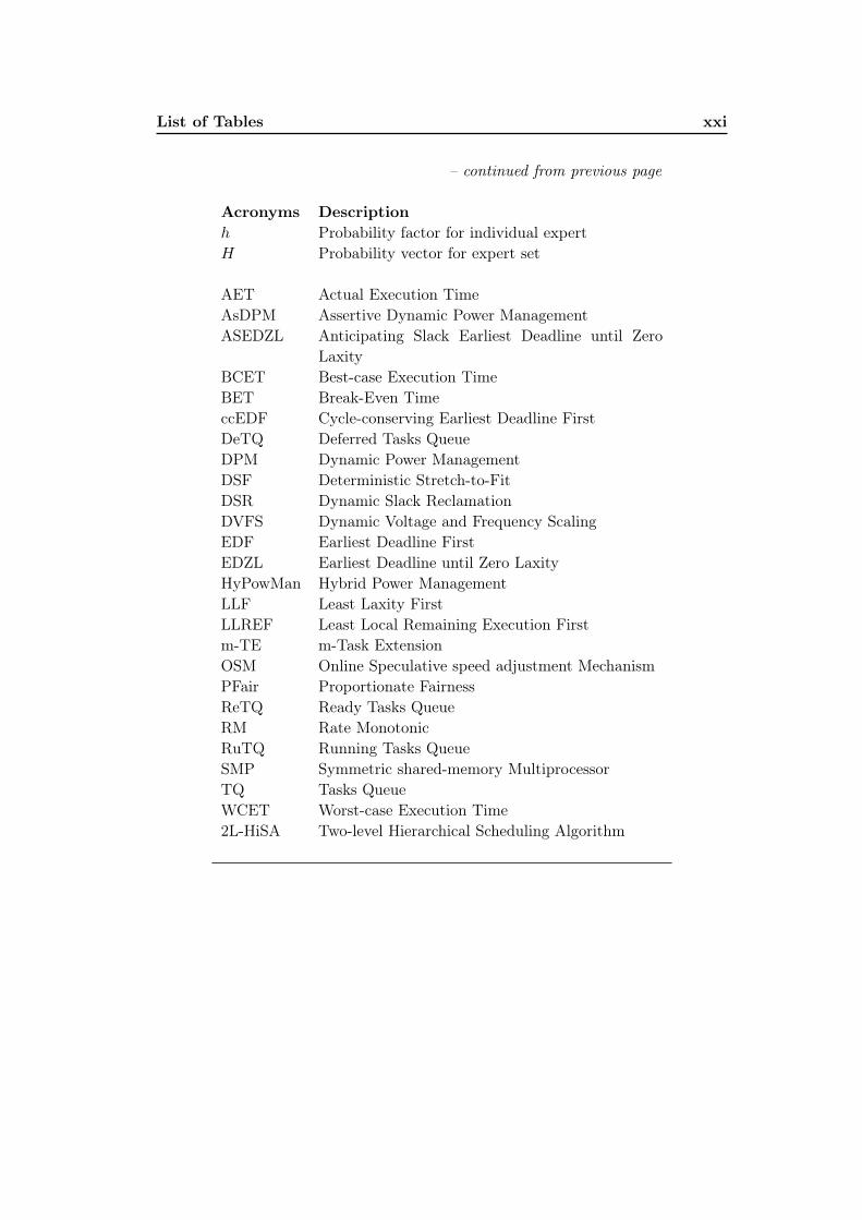
List of Tables xxi
– continued from previous page
Acronyms Descriptionh Probability factor for individual expertH Probability vector for expert set
AET Actual Execution TimeAsDPM Assertive Dynamic Power ManagementASEDZL Anticipating Slack Earliest Deadline until Zero
LaxityBCET Best-case Execution TimeBET Break-Even TimeccEDF Cycle-conserving Earliest Deadline FirstDeTQ Deferred Tasks QueueDPM Dynamic Power ManagementDSF Deterministic Stretch-to-FitDSR Dynamic Slack ReclamationDVFS Dynamic Voltage and Frequency ScalingEDF Earliest Deadline FirstEDZL Earliest Deadline until Zero LaxityHyPowMan Hybrid Power ManagementLLF Least Laxity FirstLLREF Least Local Remaining Execution Firstm-TE m-Task ExtensionOSM Online Speculative speed adjustment MechanismPFair Proportionate FairnessReTQ Ready Tasks QueueRM Rate MonotonicRuTQ Running Tasks QueueSMP Symmetric shared-memory MultiprocessorTQ Tasks QueueWCET Worst-case Execution Time2L-HiSA Two-level Hierarchical Scheduling Algorithm


Part I
Complete dissertation:English version

Chapter 1
Introduction
Contents1.1 Introduction . . . . . . . . . . . . . . . . . . . . . . . . . . . . 31.2 Contributions . . . . . . . . . . . . . . . . . . . . . . . . . . . . 51.3 Summary . . . . . . . . . . . . . . . . . . . . . . . . . . . . . . 8
1.1 Introduction
In real-time systems, the temporal correctness of produced output is equallyimportant as the logical correctness [42]. That is, real-time systems must notonly perform correct operations, but also perform them at correct time. Alogically correct operation performed by a system can result in either an erroneous,completely useless, or degraded output depending upon the strictness of timeconstraints. Based on the level of strictness of timing constraints, real-time systemscan be classified into three broad categories: hard real-time, soft real-time, andfirm real-time systems[47, 77, 105]. Such systems must be predictable and provablytemporally correct. The designer must verify that the system is correct prior toruntime –i.e., for instance, for any possible execution of a hard real-time system,each execution results in all deadlines being met. Even for the simplest systems,the number of possible execution scenarios is either infinite or prohibitively large.Therefore, exhaustive simulation or testing cannot be used to verify the temporalcorrectness of such systems. Instead, formal analysis techniques are necessary toensure that the designed systems are, by construction, provably temporally correctand predictable [42, 47]. Over the time, real-time applications have become moresophisticated and complex in their behavior and interaction. Contemporaneously,multi-core architectures have emerged to handle these sophisticated applicationsand since then, prevailed in many commercial systems. Although significantresearch has been focused on the design of real-time systems during past decades,the emergence of multi-core architectures have renewed some existing challengesas well as brought some new ones for real-time research community. Thesechallenges can be classified into three broad categories: multiprocessor platformarchitecture design, multiprocessor scheduling, and multiprocessor energy-efficiency.
As the multiprocessor architectures are already widely used, it becomes moreand more clear that future real-time systems will be deployed on multiprocessor

4 Chapter 1. Introduction
architectures. Multiprocessor architectures have certain new features that mustbe taken into consideration. For instance, application programs executing ondifferent cores usually share fine-grained resources, like shared caches, interconnectnetworks, and shared memory bandwidth, making the conventional design practicesnot suitable to multi-core systems. Thus, multi-core architectures are significantlychallenging in their design, analysis, and implementation.
Another challenge for real-time systems is the scheduling problem. The real-timescheduling problem on multiprocessor models is very different from and signifi-cantly more difficult than single-processor scheduling. Single-processor schedulingalgorithms cannot be applied on multiprocessor systems without loss of optimality.A scheduling algorithm is said to be optimal if it can successfully schedule anyfeasible task system [105]. A task system is said to be feasible if it is guaranteedthat a schedule exists that meets all deadlines of all jobs, for all sequences of jobsthat can be generated by the task system. Optimality of scheduling algorithms is acritical design issue in multiprocessor real-time systems as under-utilized platformresources are not desirable. Multiprocessor scheduling algorithms employ eithera partitioned or global scheduling approach (or hybrids of the two). Partitionedscheduling, under which tasks are statically assigned to processors and scheduledon each processor using single-processor scheduling algorithms, have low schedulingoverheads. However, the management of globally-shared resources such as a sharedmain memory and caches can become quite difficult under partitioning, preciselybecause each processor is scheduled independently. Moreover, partitioning tasksto processors is equivalent to solving a bin-packing problem: on an m-processorsystem, each task with a size equal to its utilization must be placed into one ofm bins of size one representing a processor. Bin-packing is considered a strongNP-hard problem [60]. In global scheduling algorithms, on the other hand, allprocessors select jobs to schedule from a single run queue. As a result, jobs maymigrate among processors, and contention for shared data structures is likely. Untilrecently, no multiprocessor optimal global scheduling algorithm existed before theproposition of PFair and its heuristic algorithms in [13, 106]. Although few recentlyproposed algorithms are known to be optimal [13, 106, 77, 28], multiprocessorscheduling theory has many fundamental problems still open to address.
The ever-increasing complexity of real-time applications that are being scheduledover multiprocessor architectures, ranging from multimedia and telecommunicationto aerospace applications, poses another great challenge –i.e., the power consump-tion rate of computing devices which has been increasing exponentially. Powerdensities in microprocessors have almost doubled every three years [103, 56]. Thisincreased power usage poses two types of difficulties: the energy consumption andrise in device’s temperature. As energy is power integrated over time, supplyingthe required energy may become prohibitively expensive, or even technologicallyinfeasible. This is a particular difficulty in portable systems that heavily rely onbatteries for energy, and will become even more critical as battery capacities are
1.2. Contributions 5
increasing at a much slower rate than power consumption. The energy consumedin computing devices is in large part converted into heat. With processing plat-forms heading towards 3D-stacked architectures [30, 104], thermal imbalances andenergy consumption in modern chips have resulted in power becoming a first-classdesign constraint for modern embedded real-time systems. Therefore, complex real-time systems must reduce energy consumption while providing guarantees that thetiming constraints will be met. Energy management in real-time systems has beenaddressed from both hardware and software points of view. Many software-basedapproaches, particularly scheduling-based approaches such as Dynamic Voltage andFrequency Scaling (DVFS) and Dynamic Power Management (DPM) have been pro-posed by real-time research community over the past few years. Yet their flexibilityis often matched by the complexity of the solution, with the accompanying risk thatdeadlines will occasionally be missed. As the computational demands of real-timeembedded systems continue to grow, effective yet transparent energy-managementapproaches will become increasingly important to minimize energy consumption,extend battery life, and reduce thermal effects. We believe that energy-efficiencyand scheduling of real-time systems are closely related problems, which should betackled together for best results. By exploiting the characteristic parameters ofreal-time application tasks, the energy-consciousness of scheduling algorithms andthe quality of service of real-time applications can be significantly improved. In thefollowing, we provide our thesis statement.
Thesis Statement. The goal of this dissertation is to ameliorate, throughscheduling, the energy-efficiency of real-time systems that can be proven predictableand temporally correct over multiprocessor platforms. The proposed solution(s)should be flexible to varying system requirements, less complex, and effective.Achievement of this goal implies that battery-operated real-time systems can still meettiming constraints while minimizing energy consumption, extending battery life, andreducing thermal effects.
To support our thesis, this dissertation proposes energy-aware scheduling so-lutions of complex real-time applications that are scheduled over multiprocessorarchitectures. In section 1.2, we provide an overview of each technical contributionpresented in this dissertation. A detailed background on real-time and energy-awaresystems and real-time scheduling is provided in chapter 2. Note that we review state-of-the-art related to our specific contributions in each chapter. However, relatedresearch work is also referred throughout the document where pertinent.
1.2 Contributions
Energy-efficiency in real-time systems is a multi-faceted optimization problem. Forinstance, energy optimization can be achieved at both hardware- and software-levelswhile designing the system and at scheduling-level while executing application tasks.Both the hardware and software are concerned and can play an important role inthe resulting energy consumption of overall system. In this dissertation, we focus
6 Chapter 1. Introduction
on the software-based aspects, particularly scheduling-based energy-consciousnessin real-time systems. We develop novel power and energy management techniqueswhile taking into account the features offered by existing and futuristic platformarchitectures. In the following, we discuss specific contributions presented in eachchapter of this dissertation.
Chapter 3. In this chapter, we present our first contribution which is a multi-processor scheduling algorithm, called Two-Level Hierarchical Scheduling Algorithm(2L-HiSA). This algorithm falls in the category of restricted-migration scheduling.The EDF scheduling algorithm has the least runtime complexity among job-levelfixed-priority algorithms for scheduling tasks on multiprocessor architecture. How-ever, EDF suffers from sub-optimality in multiprocessor systems. 2L-HiSA addressesthe sub-optimality of EDF as global scheduling algorithm and divides the probleminto a two-level hierarchy of schedulers. We have ensured that basic intrinsic prop-erties of optimal single-processor EDF scheduling algorithm appear in two-levelhierarchy of schedulers both at top-level scheduler as well as at local-level scheduler.2L-HiSA partitions tasks statically onto processors by following the bin-packing ap-proach, as long as schedulability of tasks partitioned on a particular processor isnot violated. Tasks that can not be partitioned on any processor in the platformqualify as migrating or global tasks. Furthermore, it makes clusters of identicalprocessors such that, per cluster, the unused fragmented computation power equiv-alent to at most one processor is available. We show that 2L-HiSA improves on theschedulability bound of EDF for multiprocessor systems and it is optimal for hardreal-time tasks if a subset of tasks can be partitioned such that the under-utilizationper cluster of processors remain less than or equal to the equivalent of one proces-sor. Partitioning tasks on processors reduces scheduling related overheads such ascontext switch, preemptions, and migrations, which eventually help reducing overallenergy consumption. The NP-hardness of partitioning problem [60], however, canoften be a limiting factor. By using clusters of processors instead of consideringindividual processors, 2L-HiSA alleviates bin-packing limitations by effectively in-creasing bin sizes in comparison to item sizes. With a cluster of processors, it ismuch easier to obtain the unused processing power per cluster less than or equal toone processor. We provide simulation results to support our proposition.
Chapter 4. Our second contribution, presented in this chapter, is a dynamicpower management technique for multiprocessor real-time systems, called AssertiveDynamic Power Management (AsDPM) technique. This technique works in con-junction with global EDF scheduling algorithm. It is an admission control techniquefor real-time tasks which decides when exactly a ready task shall execute. Withoutthis admission control, all ready tasks are executed as soon as there are enough com-puting resources (processors) available in the system, leading to poor possibilities ofputting some processors in power-efficient states. AsDPM technique differs from theexisting DPM techniques in the way it exploits the idle time intervals. Conventional
1.2. Contributions 7
DPM techniques can exploit idle intervals only once they occur on a processor –i.e.,once an idle time interval is detected. Upon detecting idle time intervals, thesetechniques decide whether to transition target processor(s) to power-efficient state.AsDPM technique, on the other hand, aggressively extracts most of the idle timeintervals from some processors and clusters them on some other processors of theplatform to elongate the duration of idle time. Transitioning processors to suit-able power-efficient state then becomes a matter of comparing idle time interval’slength against the break-even time of target processor. Although, AsDPM is anonline dynamic power management technique, its working principle can be usedto determine static optimal architecture configurations (i.e., number of processorsand their corresponding voltage-frequency level, which is required to meet real-timeconstraints in worst-case with minimum energy consumption) for target applicationthrough simulations. We demonstrate the use of AsDPM technique for both staticand dynamic energy optimization in this chapter.
Chapter 5. This chapter presents our third contribution, which is an inter-taskdynamic voltage and frequency scaling technique for real-time multiprocessor sys-tems, called Deterministic Stretch-to-Fit (DSF) technique. The DSF technique ismainly intended for multiprocessor systems. Though, applying it on single-processorsystems is also possible and in fact, rather trivial due to absence of migrating tasks.DSF comprises three algorithms, namely, Dynamic Slack Reclamation (DSR) algo-rithm, Online Speculative speed adjustment Mechanism (OSM), and m-Tasks Ex-tension (m-TE) algorithm. The DSR algorithm is the principle slack reclamationalgorithm of DSF that assigns dynamic slack, produced by a precedent task, tothe appropriate priority next ready task that would execute on the same processor.While using DSR, dynamic slack is not shared with other processors in the system.Rather, slack is fully consumed on the same processor by the task, to which it isonce attributed. Such greedy allocation of slack allows the DSR algorithm to havelarge slowdown factor for scaling voltage and frequency for a single task, whicheventually results in improved energy savings. The OSM and the m-TE algorithmsare extensions of the DSR algorithm. The OSM algorithm is an online, adaptive,and speculative speed adjustment mechanism, which anticipates early completionof tasks and performs aggressive slowdown on processor speed. Apart from sav-ing more energy as compared to the stand-alone DSR algorithm, OSM also helpsto avoid radical changes in operating frequency and supply voltage, which resultsin reduced peak power consumption, which leads to an increase in battery life forportable embedded systems. The m-TE algorithm extends an already existing One-Task Extension (OTE) technique for single-processor systems onto multiprocessorsystems. The DSF technique is generic in the sense that if a feasible schedule fora real-time target application exists under worst-case workload using (optimal ornon-optimal) global scheduling algorithms, then the same schedule can be repro-duced (using actual workload) with less power and energy consumption. Thus, DSFcan work in conjunction with various scheduling algorithms. DSF is based on the
8 Chapter 1. Introduction
principle of following the canonical execution of tasks at runtime –i.e., an offline orstatic optimal schedule in which all jobs of tasks exhibit their worst-case executiontime. A track of the execution of all tasks in static optimal schedule needs to bekept in order to follow it at runtime [10]. However, producing and keeping an entirecanonical schedule offline is impractical in multiprocessor systems due to a prioriunknown assignment of preemptive and migrating tasks to processors. Therefore,we propose a scheme to produce an online canonical schedule ahead of practicalschedule, which mimics the canonical execution of tasks only for future m-tasks.This reduces scheduler’s overhead at runtime as well as makes DSF an adaptivetechnique.
Chapter 6. While new energy management techniques are still developed to dealwith specific set of operating conditions, recent research reports that both DPMand DVFS techniques often outperform each other when their operating conditionschange [37, 20]. Thus, no single policy fits perfectly in all or most operating con-ditions. Our fourth and final contribution in this dissertation addresses this issue.We propose, in this chapter, a generic power and energy management scheme formultiprocessor real-time systems, called Hybrid Power Management (HyPowMan)scheme. This scheme serves as a top-level entity that, instead of designing new pow-er/energy management policies (whether DPM or DVFS) for specific operating con-ditions, takes a set of well-known existing policies. Each policy in the selected policyset, when functions as a stand-alone policy, ensures deadline guarantees and per-forms well for a given set of operating conditions. At runtime, the best-performingpolicy for given workload is adapted by HyPowMan scheme through a machine-learning algorithm. This scheme can enhance the ability of portable embeddedsystems to adapt with changing workload (and platform configuration) by workingwith a larger set of operating conditions and gives overall performance and energysavings that are better than any single policy can offer.
Chapter 7. In this chapter, we provide general conclusions and remarks on ourcontributions and results. Moreover, we discuss some future research perspectivesof this dissertation.
Appendixes. We provide two appendixes in this dissertation. Appendix A pro-vides functional details on the simulation tool STORM (Simulation TOol for Real-time Multiprocessor scheduling) [108] that we use in our simulations throughout thisdissertation. Appendix B provides some additional simulation results related tochapter 6.
1.3 Summary
As a result of contemporaneous evolution in the complexity and sophistication ofreal-time applications and multiprocessor platforms, the research on real-time sys-
1.3. Summary 9
tems has confronted with many emerging challenges. One such challenge that real-time research community is facing is to reduce power and energy consumption ofthese systems, while maintaining assurance that timing constraints will be met.As the computational demands of real-time systems continue to grow, effective yettransparent energy-management approaches are becoming increasingly importantto minimize energy consumption, extend battery life, and reduce thermal effects.Power- and energy-efficiency and scheduling of real-time systems are closely relatedproblems, which should be tackled together for best results. Our dissertation mo-tivates this thesis and attempts to address together the problem of overall energy-awareness and scheduling of multiprocessor real-time systems. This dissertationproposes novel approaches for energy-management within the paradigm of energy-aware scheduling for soft and hard real-time applications, which are scheduled overidentical multiprocessor platforms of type symmetric shared-memory multiproces-sor (SMP). We believe that by exploiting the characteristic parameters of real-timeapplication tasks, the energy-consciousness of scheduling algorithms and the qual-ity of service of real-time applications can be significantly improved. Rest of thisdocument provides our contributions in detail.


Chapter 2
Background on Real-time andEnergy-efficient Systems
Contents2.1 Real-time Systems . . . . . . . . . . . . . . . . . . . . . . . . . 11
2.1.1 Real-time Workload . . . . . . . . . . . . . . . . . . . . . . . 122.1.2 Processing Platform . . . . . . . . . . . . . . . . . . . . . . . 162.1.3 Real-time Scheduling . . . . . . . . . . . . . . . . . . . . . . . 172.1.4 Real-time Scheduling in Multiprocessor Systems . . . . . . . 20
2.2 Power- and Energy-efficiency in Real-time Systems . . . . . 232.2.1 Power and Energy Model . . . . . . . . . . . . . . . . . . . . 232.2.2 Energy-aware Real-time Scheduling . . . . . . . . . . . . . . . 26
2.3 Simulation Environment . . . . . . . . . . . . . . . . . . . . . 282.4 Summary . . . . . . . . . . . . . . . . . . . . . . . . . . . . . . 29
2.1 Real-time Systems
Real-time systems can be classified, based on the strictness of timing constraints,into three broad categories: hard real-time, soft real-time and firm real-time systems[42, 47, 77, 80, 105].
Hard real-time systems. In hard real-time systems, the completion of a correctoperation after its deadline is considered as useless. Ultimately, this operation maycause a critical failure of the system or expose end-users to hazardous situations. Inother words, the penalty for even a single temporal constraint violation is unaccept-able in hard real-time systems. Aerospace, nuclear, power plant, and automobileapplications would use such systems.
Soft real-time systems. Soft real-time systems lower their strictness of timingconstraints as compared to hard real-time systems. In such systems, although itis still preferred to have operations completed before their deadlines, violation oftiming constraints does not make produced outputs entirely useless or hazardous.Even if deadlines of most operations are missed, the system can continue to oper-ate. Such systems are nonetheless referred to as real-time since they use real-time
12 Chapter 2. Background on Real-time and Energy-efficient Systems
mechanisms (such as real-time operating systems for instance) in order to meet asmany deadlines as possible. Cellular phone and multimedia applications can usesuch systems as the consequences of missing deadlines could be smaller than thecost of meeting them in all possible circumstances.
Firm real-time systems. Firm real-time systems provide an intermediateparadigm between hard and soft real-time systems. In contrast to hard real-timesystems, firm real-time systems tolerate some latency in operations –i.e., a deadlinemiss results only in a decreased quality of service. Basically, the notion of firm real-time is less strict than that of hard real-time since it allows deadlines to be missed,but it is more strict than soft real-time in the sense that only a predefined ratioof deadline miss is allowed. Systems such as flight ticketing data servers that re-quire concurrency, but can afford a delay in seconds, may use firm real-time systems.
As mentioned in section 1.1, a real-time system must ensure that, by construc-tion, it is provably temporally correct and predictable. A real-time system can beproven predictable and temporally correct by specifying the following three aspects.Firstly, the real-time workload –i.e., the computation produced by a real-time ap-plication that must complete prior to its deadline, is specified in the form of tasks.These tasks are often recurring in their nature in real-time systems. Secondly, theprocessing platform or hardware resources upon which the application tasks are ex-ecuted. Thirdly, a scheduling algorithm that determines, at any time, which setof tasks execute on the processing platform. In the following, we discuss all threeaspects in more detail.
2.1.1 Real-time Workload
Real-time applications have become more sophisticated and complex in their behav-ior and interaction over the time [3]. As mentioned in earlier section, an applicationis said to be real-time when it is subject to timing constraints for its individualjobs/events as well as for its overall system response. These timing constraints areusually applied by the system designer, however, they typically reflect a need forsafety or sustainability of the system performance. Definition of these timing con-straints categorize an application into hard real-time, soft real-time, or firm real-timeapplications. For instance, the ABS breaking system in cars and video streamingapplications are good examples of hard and soft real-time systems, respectively.Typically, hard real-time applications work in closed and highly predictable envi-ronments. On the contrary, soft real-time applications execute in open and lesspredictable environments.
In real-time systems, a common assumption is that it is possible to decompose areal-time application into a finite set of discrete tasks. Each task represents certainfunctionality of application. These tasks possess certain characteristic parameterssuch as release instant, periodicity, deadline, and execution requirement. Based onthese parameters, tasks may be specified according to different task models. A task
2.1. Real-time Systems 13
model is the format and rules for specifying a task system. Before elaborating dif-ferent task models, we present these characteristic parameters, which are associatedwith real-time tasks. From now on, we say that a task Ti releases a job Ti,j (wherej is the index of the job) at time instant t to express the fact that Ti is instantiatedexactly at instant t so that its treatment can be carried out. A job can therefore beseen as an instance of a task Ti. In the following, we recall classical definitions forcertain parameters that characterize tasks of real-time applications.
Deadline (di) of a real-time task is one of the key parameters which reflects thetiming constraint on its execution. This quantity can be expressed as a numberof CPU clock cycles but other reference units can be used, such as CPU ticks forinstance. Hereafter, we use the term time unit to refer to the used reference unit.In this dissertation, deadline will denote the relative deadline of Ti –i.e., relative toits last job release, with the interpretation that once the task releases a job, thatjob must be completely executed by di time units.
Period (Pi) of a real-time task in another key parameter which reflects thedelay between two consecutive job releases of task Ti. This parameter can beinterpreted in three distinct ways, each of which leads to a well-defined type oftask. According to the interpretation given to the period, tasks can be classifiedinto three categories of task models: periodic task model, sporadic task model, andaperiodic task model. We elaborate further these task models in section 2.1.1.1.
Note that, very often, the theoretical results proposed in the literature applyonly to tasks that provide a particular relation between their period and deadline.Therefore, it is worth mentioning the specific vocabulary that characterizes suchrelations. Ti is said to be constrained-deadline task if di ≤ Pi or implicit-deadlinetask in the particular case where di = Pi. When the proposed result holds whateverthe relation between period and deadline, Ti is said to be arbitrary-deadline task.Note that the following inclusion holds: an implicit-deadline task is a constrained-deadline task which is in turn an arbitrary-deadline task. Thanks to this inclusiverelation between the task models, any property that holds for an arbitrary-deadlinetask also holds for a constrained- and implicit-deadline task.
Offset (Oi) refers to the time delay before the release time of the first job of aperiodic real-time task. In other words, the offset corresponds to the release timeof the first job Ti,1 of task Ti. When the whole application is modeled by a singleset of tasks with identical offsets, the application is said to be synchronous; withoutloss of generality, the offset of every task can be considered as 0 and can be ignored.Otherwise, if the offsets for different tasks are not equal, the application is saidto be asynchronous. Notice that the offset of a task is defined only if the task isperiodic. This is because the release times of the jobs (including the first one) forsporadic/aperiodic tasks are not known beforehand.
14 Chapter 2. Background on Real-time and Energy-efficient Systems
Worst-case execution time (Ci) refers to the largest execution time needed tocomplete a distinct job of a task Ti, assuming that its execution is not interrupted.Since real-time systems are designed to achieve only a few specific functions on aspecific processing platform, mostly it is assumed that the Worst-Case ExecutionTime (WCET) of every task is known beforehand. WCET of a task is usuallyexpressed in the same units as deadline and period. Note that the value of Cidepends not only on the functional code of Ti, but varies on different platforms.Authors in [123] suggest that the estimated WCET of tasks must offer both tightnessand safety properties. Tightness means that they must be as close as possible to theactual WCET of a task, not to overestimate the resources required by the system.Safety is the guarantee that the computed WCET is greater than or equal to anypossible execution time. The process of determining Ci must account for issues likeworst-case cache behavior, pipeline stalls, memory contention, memory access time,program structure, and worst-case execution paths within the code.
There are some other factors as well, which are not directly concerned withthe estimation of WCET, but contribute to the response time of tasks such as jobpreemptions, context switching, state saving, and scheduling-decision processingtime by operating system. If a job is allowed to migrate between processors duringits scheduling window, there may be an added penalty of refreshing the cache of theprocessor, to which the job is migrating. The preemption and migration costs aretypically dependent on the processor architecture and the scheduling algorithm.
Within the scope of this dissertation, we consider that the WCET of all tasksis known beforehand. Interested reader may refer to some recent research work andsurveys presented in [123, 69, 70] for further investigations in this research field.
Laxity (Li) is a runtime parameter of a task’s job that is a measure of its urgencyto execute relative to its deadline. For instance, in a feasible task set, a job withzero laxity is the most urgent job to execute in order to avoid deadline miss. Theabsolute laxity (Li) of a task at its release time instant t is given by equation 2.1.
Li = di − (t+ Ci) (2.1)
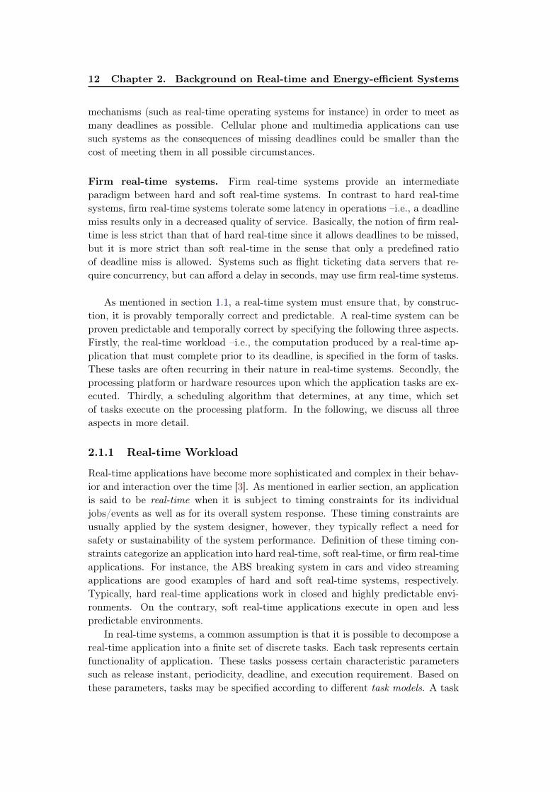
Figure 2.1 illustrates a sample schedule of tasks and graphical representationof various characteristic parameters. This figure illustrates the schedule of a singleperiodic task Ti having implicit deadline –i.e., di=Pi, on a single processor. Theparameters of Ti are: Oi=2, Ci=3, and di=Pi=4. Each green box represents a job oftask Ti and its length corresponds to its worst-case execution time Ci. The releaseand deadline time instants are represented by up and down arrows, respectively.According to the definitions above, Ti releases a job noted Ti,j (∀j, j=1, 2, ...,∞)at each instant ri. Each such job has a WCET of Ci and it must complete by itsrelative deadline noted di. At release instant, a task has an absolute laxity of Li.
2.1. Real-time Systems 15
Figure 2.1: Illustration of various characteristic parameters of real-time tasks. Pe-riodic task Ti has an implicit deadline (di=Pi) with the following values of otherparameters. Oi=2, Ci=3, di=Pi=4, and Li=1.
2.1.1.1 Task models
Based on the knowledge of characteristic parameters presented in section 2.1.1, webriefly discuss various classical task models in the following.
Periodic Task Model: This task model, presented by Liu and Layland in [71],allows the specification of homogeneous sets of jobs that recur at strict periodicinterval. A periodic task Ti is specified by its offset, WCET, and period. Note thatfor such task models, every task has an exact inter-arrival time between successivejobs. Along with this interpretation, it is often assumed that the release time of thevery first job of the tasks is also known beforehand, thus implying that the exactrelease time instants of every job can be computed at the system design-time.
Sporadic Task Model: The sporadic task model with implicit deadlines, pre-sented by Liu and Layland in [71], removes the restrictive assumption of generatingjobs at strict periodic intervals of time. In addition, an offset parameter is notspecified for sporadic tasks. The behavior of a sporadic task Ti can be character-ized by only the WCET and its period. The parameter Pi indicates the minimuminter-arrival time between successive jobs of Ti (note that Pi denoted the exactinter-arrival time for periodic tasks). That is, the exact release time of every job isnot known before they are actually released at runtime.
Aperiodic Task Model: In this task model, the tasks do not have a periodparameter. That is, system designers have no prior information about the time-instants at which jobs are released.
2.1.1.2 Description of workload model in this dissertation
Throughout this dissertation, we characterize a periodic and independent taskset τ as a finite collection of tasks such that τ = {T1, T2, Ti, ..., Tn−1, Tn}, and
16 Chapter 2. Background on Real-time and Energy-efficient Systems
a real-time task Ti composed of a finite or infinite collection of jobs such thatJ = {Ti,1, Ti,2, ...}. The letter n will denote the number of tasks in a task set. Everyjob Ti,j of a real-time task Ti, (∀i, 1 ≤ i ≤ n) will be characterized by the quadruplet(ri, Ci, di, Pi): an arrival or release time ri, a worst-case execution requirement Ci,a relative deadline di, and a period Pi. The interpretation of these parameters isthat the job Ti,j of a task Ti arrives after ri time units after the system start-time(the offset will be assumed zero in our general system model) and must executefor Ci time units over the time interval [ri, ri + di). Release instant ri is assumedto be a non-negative real number while both Ci and di are positive real numbers.The interval [ri, ri + di) is referred to as Ti,j ’s scheduling window. A job Ti,j is saidto be active at time instant t if t ∈ [ri, ri + di) and Ti,j has unfinished execution.In general task model, we consider a completely specified system –i.e., the systemdesigner has complete knowledge of each job Ti,j and infinitely-repeating jobs aregenerated by independent periodic tasks. We consider an implicit deadline taskmodel. Furthermore, we consider that preemption of tasks –i.e., a job suspendswhile a different job executes and resumes execution at later time, is allowed. In allfigures that illustrate scheduling of tasks throughout this dissertation, an upwardarrow indicates a job’s release and a downward arrow indicates its deadline andperiod. A rectangular box on the time line indicates that a task is executing duringthat interval as illustrated in figure 2.1.When analyzing a system, we need to know the execution requirement of eachtask –i.e., the amortized amount of processing time the task will need. A task’sutilization can be used to measure its processing requirement. The utilization oftask Ti is the proportion of processing time the task will require if it is executedon a unit-speed (ν) processor: ui
def= Ci/Pi. The aggregate utilization of a periodic
task set, Usum (τ)def=∑n
i=1 ui, measures the proportion of processor’s time theentire task set will require.
In the rest of this dissertation, we consider that the worst-case execution timeof tasks is known a priori, all jobs of tasks are preemptable, full migration of tasksis allowed (except in case of chapter 3), task-level parallelism is allowed, however,job-level parallelism is not permitted (i.e., a job may not execute concurrently withitself on multiple processors), and tasks are independent of each other –i.e., theexecution of one task’s job is not contingent upon the status of another task’s job.Blocking of shared resources in not permitted as well.
2.1.2 Processing Platform
A complete real-time system is a real-time task model paired with a specific pro-cessing platform, which has a specific computing capacity. The platform may becomposed of a single processor denoted by π or it may contain multiple processorsdenoted by Π such that Π = {π1, π2, ..., πm}. Letter m refers to the number ofprocessors in a multiprocessor platform. If the platform is a multiprocessor, theindividual processors may all be the same (identical) or they may differ from one

2.1. Real-time Systems 17
another. As highlighted by authors in [3, 4], multiprocessor platforms are more en-ergy efficient than equally powerful single-processor platforms, because raising thefrequency of a single processor results in a multiplicative increase of the energy con-sumption while adding processors leads to an additive increase. More details arepresented in section 2.2. In the following, we discuss certain categories of multipro-cessor systems which differ from one another based on the speeds of the individualprocessors.
Unrelated multiprocessor platform. In these platforms, the processing speeddepends not only on the processor, but also on the job being executed. In suchplatforms, a specific speed is associated to every processor-task couple with theinterpretation that, in any time interval of length L, task Ti executes ν×L executionunits when executed on processor πk. This model of platform was introduced inorder to reflect the fact that two distinct tasks (i.e., with different code-instructions)executed on the same processor can require different execution times to completeeven though the length of their code is identical. This is due to internal architectureof the processors and the type of the task instructions. Indeed, some processors areoptimized for some types of instructions while they require more time to completeother types of instructions.
Uniform multiprocessor platform. In these platforms, the processing speeddepends only on the processor. For instance, considering two different jobs, for allpairs of jobs Ti,j and Ti,j+1 that execute on the same processor πk, the processorspeed remains the same.
Identical multiprocessor platform. In these platforms, all processors havethe same speeds. Generally, in such systems, the speed is usually normalized toone unit of work per unit of time. The identical multiprocessor platform modelconsiders that all the processors have the same characteristics, in term of powerconsumption, computational capabilities, architecture, cache size and speed, I/Oand resource access, and access time to shared memory etc. In any interval of time,two identical processors execute the same amount of work and consume the sameamount of energy.
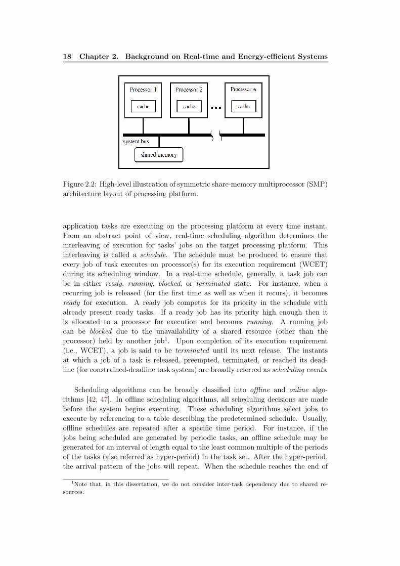
In this dissertation, we consider an identical multiprocessor platforms forscheduling real-time tasks. Precisely, we consider symmetric shared-memory multi-processor (SMP) layout of multiprocessor identical platform as illustrated in figure2.2.
2.1.3 Real-time Scheduling
Real-time scheduling is one of the three aspects that should be taken into accountto prove predictability and temporal correctness of real-time systems. The roleof a real-time scheduling algorithm is to determine which active jobs of real-time
18 Chapter 2. Background on Real-time and Energy-efficient Systems
Figure 2.2: High-level illustration of symmetric share-memory multiprocessor (SMP)architecture layout of processing platform.
application tasks are executing on the processing platform at every time instant.From an abstract point of view, real-time scheduling algorithm determines theinterleaving of execution for tasks’ jobs on the target processing platform. Thisinterleaving is called a schedule. The schedule must be produced to ensure thatevery job of task executes on processor(s) for its execution requirement (WCET)during its scheduling window. In a real-time schedule, generally, a task job canbe in either ready, running, blocked, or terminated state. For instance, when arecurring job is released (for the first time as well as when it recurs), it becomesready for execution. A ready job competes for its priority in the schedule withalready present ready tasks. If a ready job has its priority high enough then itis allocated to a processor for execution and becomes running. A running jobcan be blocked due to the unavailability of a shared resource (other than theprocessor) held by another job1. Upon completion of its execution requirement(i.e., WCET), a job is said to be terminated until its next release. The instantsat which a job of a task is released, preempted, terminated, or reached its dead-line (for constrained-deadline task system) are broadly referred as scheduling events.
Scheduling algorithms can be broadly classified into offline and online algo-rithms [42, 47]. In offline scheduling algorithms, all scheduling decisions are madebefore the system begins executing. These scheduling algorithms select jobs toexecute by referencing to a table describing the predetermined schedule. Usually,offline schedules are repeated after a specific time period. For instance, if thejobs being scheduled are generated by periodic tasks, an offline schedule may begenerated for an interval of length equal to the least common multiple of the periodsof the tasks (also referred as hyper-period) in the task set. After the hyper-period,the arrival pattern of the jobs will repeat. When the schedule reaches the end of
1Note that, in this dissertation, we do not consider inter-task dependency due to shared re-sources.
2.1. Real-time Systems 19
the predetermined table, it can simply return to the beginning of the table. Inonline scheduling algorithms, on the other hand, all scheduling decisions are madewithout specific knowledge of jobs that have not yet arrived. These schedulingalgorithms select jobs to execute by examining properties of active jobs. Onlinealgorithms can be more flexible than offline algorithms since they can schedule jobswhose behavior cannot be predicted ahead of time. Online scheduling algorithmscan be divided into fixed-priority and dynamic-priority scheduling algorithms.
In fixed-priority scheduling algorithms, all jobs generated by the same taskhave the same priority. More formally, if job Ti,j has higher priority than Tl,j thenTi,j+1 has higher priority than Tl,j+1 for all values of j. Fixed-priority algorithmsalso referred as Static-priority algorithms. One very well-known fixed-priorityscheduling algorithm is the Rate Monotonic (RM) algorithm proposed by [71].In this algorithm, the task period is used to determine priority –i.e., tasks withshorter periods have higher priority. This algorithm is known to be optimal amongsingle-processor fixed-priority algorithms –i.e., if it is possible for all jobs to meettheir deadlines using a fixed priority algorithm, then they will meet their deadlineswhen scheduled using RM algorithm. In dynamic-priority scheduling algorithms,jobs generated by the same task may have different priorities. The Earliest DeadlineFirst (EDF) algorithm [23, 71, 85] is a well-known dynamic-priority algorithm. EDFscheduling algorithm is optimal among all single-processor scheduling algorithms–i.e., if it is possible for all jobs to meet their deadlines, they will do so whenscheduled using EDF. Dynamic-priority algorithms can be further divided into twocategories –i.e., job-level fixed-priority and job-level dynamic-priority algorithms,depending on whether individual jobs can change priority while they are active.In job-level fixed-priority algorithms, jobs cannot change priorities. EDF is ajob-level fixed-priority algorithm. On the other hand, in job-level dynamic-priorityalgorithms, jobs may change priority during execution. Least Laxity First (LLF)algorithm [33, 71] is a job-level dynamic-priority algorithm. LLF schedulingalgorithm assigns a higher priority to a task with smaller laxity and it has beenknown as an optimal preemptive scheduling algorithm on a single processor platform.
Another important aspect of scheduling algorithms is their optimality. Ascheduling algorithm is said to be optimal if it can successfully schedule any feasibletask system. A task system is said to be feasible if it is guaranteed that a schedule ex-ists that meets all deadlines of all jobs, for all sequences of jobs that can be generatedby the task system. For instance, EDF is an optimal scheduling algorithm for single-processor systems [85] whereas, Rate monotonic (RM) is not an optimal algorithmfor all single-processors. RM is optimal on single-processor systems only amongfixed-priority algorithms –i.e., if it is possible for a task set to meet all deadlines us-ing a fixed-priority algorithm then that task set is RM-schedulable [85]. Authors in[71] proved that for a set of n periodic tasks with unique periods, a feasible schedulethat will always meet deadlines exists if the aggregate utilization of tasks is belowa specific bound depending on the number of tasks –i.e.,
∑ni=1 ui ≤ n
(n√
2− 1).

20 Chapter 2. Background on Real-time and Energy-efficient Systems
When the number of tasks tends towards infinity, the schedulable utilization of RMalgorithms tends towards a constant value –i.e., n→∞;
∑ni=1 ui ≈ 0.693. Authors
in [21] propose a hyperbolic bound relative to the Liu and Layland bound [71] andshow that for n tending to infinity, the hyperbolic bound was found to be equal to√
2. Single-processor systems that allow dynamic-priority scheduling will commonlyuse the EDF scheduling algorithm, while systems that can only use fixed-priorityscheduling algorithms will use the RM scheduling algorithm. Since the focus of thisdissertation is mainly on multiprocessor real-time systems, therefore, we discuss inthe following how scheduling problem in multiprocessor systems is addressed.
2.1.4 Real-time Scheduling in Multiprocessor Systems
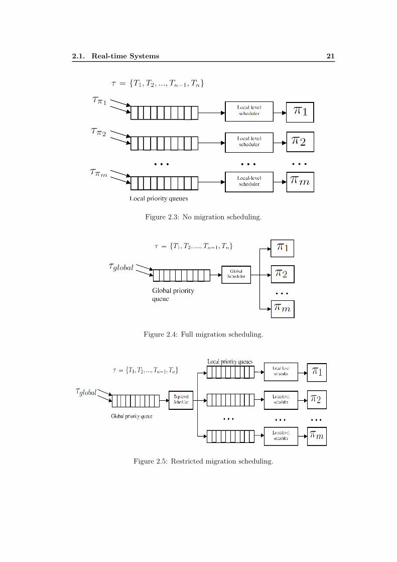
In multiprocessor systems, the problem of scheduling tasks is typically solved usingdifferent approaches based on how much migration the system allows at runtime.A task is said to be migrating if its successive jobs (or parts of the same job) areexecuted on different processors. Based on the amount of allowable migration,three types of migration strategies can be considered [8, 42, 47, 63].
No Migration. In this type of scheduling strategies, tasks can never migrate.Each task is statically assigned to a specific processor before execution and, atruntime, all job instances generated by a task execute on the processor to which,the task is assigned. Figure 2.3 illustrates a partitioned scheduler in which,every processor maintains a unique priority space associated only with the tasksbeing partitioned on it. No migration strategies are also referred as partitionedscheduling strategies. Partitioned scheduling approach has the virtue of permittingschedulability of task set to be verified using well-established single-processorschedulability analysis techniques.
Full Migration. In this type of scheduling strategies, jobs of a task can migrateat any point in time during their execution. All jobs are permitted to execute on anyprocessor of the system. However, a job can only execute on at most one processorat a time –i.e., job parallelism is not permitted. Figure 2.4 illustrates a full migra-tion scheduling in which, a single priority space is associated with all processors inthe system. Full migration strategies are also referred as global scheduling strategies.
Restricted Migration. In this type of scheduling strategies, tasks can migrateonly at job boundaries. Whenever a new job of a task is released, a top-levelscheduler assigns this job to a particular processor. Once assigned, this job mustcomplete its execution on the processor to which it is assigned –i.e., it can notmigrate. However, the next job of the same task can execute on the same or differentprocessor. Once assigned, the execution of job is the responsibility of the localscheduler on that processor. Figure 2.5 illustrates a restricted migration schedulerin which, there is a global priority queue and local priority queues for each processor.
2.1. Real-time Systems 21
Figure 2.3: No migration scheduling.
Figure 2.4: Full migration scheduling.
Figure 2.5: Restricted migration scheduling.

22 Chapter 2. Background on Real-time and Energy-efficient Systems
Prohibiting migration, as in case of partitioned scheduling, may cause a systemto be under-utilized [8, 47] and for that reason, more than enough processing powerwill be available on some processor when a new job arrives. If migration is allowed,on the other hand, the job can execute for some time on one processor and then moveto another processor, allowing the spare processing power to be distributed amongall the processors. However, while full migration strategy is the most flexible, thereare clearly overheads associated with allowing migration such as increased contextswitching, handling of shared resources, and cache-related overhead etc. Thus, thereis a trade-off between scheduling loss due to migration and scheduling loss due toprohibiting migration.
2.1.4.1 Earliest Deadline First (EDF) as multiprocessor real-timescheduling algorithm
In this dissertation, EDF scheduling algorithm is often used to schedule real-timetasks on multiprocessor platform. In this section, we present EDF as a multi-processor real-time scheduling algorithm. EDF is a job-level fixed-priority onlinescheduling algorithm which is optimal for single-processor systems [23, 71]. Au-thors in [34, 52] have shown that, for multiprocessor systems, there is no job-levelfixed-priority optimal online scheduling algorithm. Since EDF is a job-level fixed-priority scheduling algorithm for multiprocessors, determining whether a given taskset is feasible on a multiprocessor platform will not tell us whether that task setis EDF-schedulable on the same platform as well. Thus, EDF is not optimal formultiprocessor systems. Nonetheless, there are still many compelling reasons forusing EDF for scheduling real-time applications on multiprocessor systems.
• Since EDF is an optimal single-processor scheduling algorithm, therefore, alllocal scheduling decisions are taken using an optimal algorithm when EDF isused in partitioning and restricted-migration based systems.
• EDF is considered as efficient from implementations point of view [74].
• The number of preemptions and migrations incurred by EDF can be bounded.Bounds depend on which migration strategy is being used. Since migrationand preemption both incur overheads, it is important to be able to incorporatethe overheads into any system analysis. This can only be done if the associatedoverheads can be bounded [52, 47].
On single-processor, EDF is well defined –i.e., for execution at every time in-stant, the job that has the smallest deadline is selected for execution on the soleprocessor. EDF is optimal scheduling algorithm for single-processo systems. Whenmore processors are added to the system, however, EDF suffers from sub-optimality.The utilization bound for periodic tasks with implicit deadlines under EDF multi-processor scheduling algorithm cannot be higher than (m+1)
2 for an m-processorplatform [7]. This is a sufficient condition bound. One of the contributions of this
2.2. Power- and Energy-efficiency in Real-time Systems 23
dissertation (in chapter 3) is to increase this schedulability bound of EDF algorithmusing restricted-migration strategy.
2.2 Power- and Energy-efficiency in Real-time Systems
The demand for portable systems is ever-increasing with more complex functionalityrequirements as depicted in figure 2.6(a). The assessment of ITRS (InternationalTechnology Road map for Semiconductors) in 2008 fore casted further increase inpower consumption in cell phones (see figure 2.6(b)). EPoSS (the European Tech-nology Platform on Smart Systems Integration) suggested in 2009 that the energydensity in batteries would increase beyond 400 Wh/kg by 2020 (see figure 2.6(c)).All these assessments suggest that complex real-time systems, which are composed ofsophisticated real-time applications being scheduled over multiprocessor platforms,must be increasingly challenged to reduce energy consumption while maintainingassurance that timing constraints will be met. Power and energy in these complexsystems is managed at both system design-time as well as runtime. In a post-designscenario, energy saving is achieved by static (offline) optimizations as well as byactively changing the power consumption profile of the system at runtime (online).
2.2.1 Power and Energy Model
There are two principle sources of power dissipation in CMOS (ComplementaryMetal-Oxide Semiconductor) technology-based systems: dynamic power dissipation,which arises from the repeated capacitance charge and discharge on the output ofthe hundreds of millions of gates in modern chips, and static power dissipation whicharises from the electric current that leaks through transistors even when they areturned off. Until very recently, only dynamic power dissipation has been a significantsource of power consumption. However, shrinking processor technology below 100
nanometer has allowed and actually required reducing the supply voltage. Reducedfeature-size favors dynamic power dissipation but unfortunately, smaller geometriesexacerbate leakage, so static power begins to dominate the power consumption indeep sub-micron technology. Overall power consumption of CMOS technology-basedprocessors, represented as a function of speed (ν) in variable speed settings, iscomposed of static and dynamic components which relate to supply voltage Vop,operating frequency Fop, and leakage current (Iq) through an approximate relationgiven by equation 2.2.
Pwr(ν) = γCeffV2opFop + IqVop (2.2)
Here, γ is the fraction of gates actively switching and Ceff refers to the totalload capacitance of all gates. The first addend in equation 2.2 corresponds to dy-namically dissipated power and second addend models statically dissipated power.We have ignored power lost to the momentary short circuit that occurs at the out-put whenever the switching activity takes place. The loss is relatively small; it
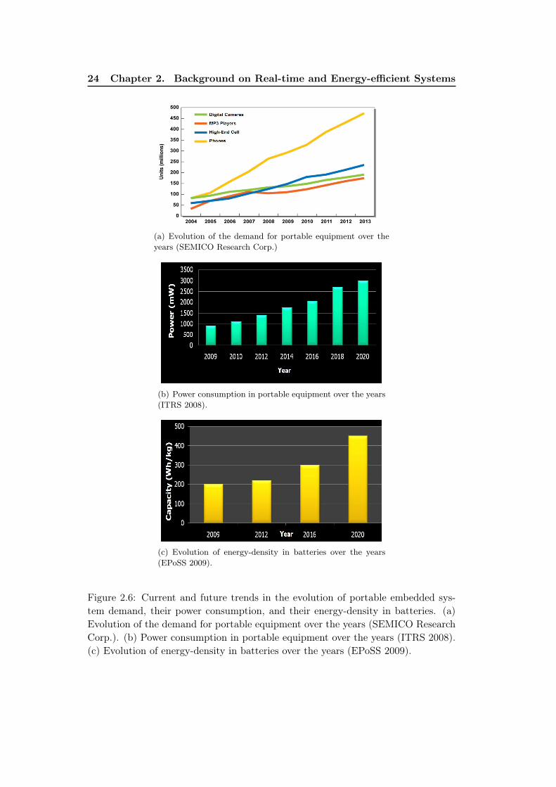
24 Chapter 2. Background on Real-time and Energy-efficient Systems
(a) Evolution of the demand for portable equipment over theyears (SEMICO Research Corp.)
(b) Power consumption in portable equipment over the years(ITRS 2008).
(c) Evolution of energy-density in batteries over the years(EPoSS 2009).
Figure 2.6: Current and future trends in the evolution of portable embedded sys-tem demand, their power consumption, and their energy-density in batteries. (a)Evolution of the demand for portable equipment over the years (SEMICO ResearchCorp.). (b) Power consumption in portable equipment over the years (ITRS 2008).(c) Evolution of energy-density in batteries over the years (EPoSS 2009).
2.2. Power- and Energy-efficiency in Real-time Systems 25
contributes to dynamic power dissipation, and the first term in equation 2.2 canabsorb it, if necessary.
When dynamic power is the dominant source of power consumption –as it hasbeen historically in many less aggressive fabrication technologies– it is possible toapproximate equation 2.2 with just the first term. In that case, the relation ofV 2op suggests reducing supply voltage as the most effective way to decrease power
consumption. For instance, halving the voltage will reduce the power consumptionby a factor of four. Supply voltage is also related to the operating frequency of theprocessors by the relationship given in equation 2.3.
Fop ≈(Vop − Vth)η
Vop(2.3)
Where Vth is the threshold or switching voltage and the exponent η is an ex-perimentally derived constant that depends on the technology in use. During thepast decades, the threshold voltage of the manufactured devices was too high togenerate a significant leakage current when the state of the device is off, but stilllow enough compared to Vop to be ignored in the above expression. That is, theexpression above could be rewritten as in equation 2.4.
Fop ≈ (Vop)η−1 (2.4)
For instance, in technology based on classical MOSFETs (Metal-Oxide Semicon-ductor Field Effect Transistor), η= 2 [80], making the frequency a linear functionof the supply voltage. However, the exact knowledge of η is not essential. The mostimportant feature is the fact that the power function Pwr(ν) is a strictly increasingconvex function of the frequency. Historically, CMOS technology has dissipatedmuch less power. In fact, when not switching, CMOS transistors lost negligible(static) power. However, the power they consume has increased dramatically withincreases in device speed and chip density. Continuously shrinking transistor sizehave forced a reduction of the threshold voltage as well. This miniaturizationreduces the gap between the supply voltage and threshold voltage, resulting in asignificant sub-threshold leakage current. Nowadays, these leakage currents arebecoming a significant factor to portable devices because of their undesirable effecton battery life time. Hence, static power dissipation can no more be ignored inmodern embedded systems. In this dissertation, we consider that static power is asignificant contributing factor to overall power and energy dissipation and cannotbe ignored any further.
Although power-efficiency and energy-efficiency are often perceived as overlap-ping goals, there are certain differences when designing systems for one or the other.Formally, the energy consumed by a system is the amount of power dissipated dur-ing a certain period of time. For instance, if a task occupies a processor during anexecution interval of [t1, t2] then the energy consumed by the processor during thistime interval is given by equation 2.5.
26 Chapter 2. Background on Real-time and Energy-efficient Systems
E[t1, t2] =
∫ t2
t1
Pwr(ν(t))dt (2.5)
Equation 2.5 shows that there is an aspect of time involved in energy consump-tion of the system. Every computation operation requires a specific interval of timeto be completed. The energy consumption decreases if the time required to performsuch operation decreases and/or the power consumption decreases. For instance,power can be halved by simply halving the operating frequency, but at the sametime, overall computation time would be doubled, which might be leading to no ef-fect on overall energy consumption. Thus, a technique that would purely minimizepower dissipation, but at the same moment increase the computational time, mightlead to non change or even an increase in energy consumption.
Power- and energy-efficiency and scheduling of real-time systems are thereforeclosely related problems, which should be tackled together for best results. This dis-sertation is an attempt to address together the problem of overall energy-awarenessand scheduling of multiprocessor real-time systems.
2.2.2 Energy-aware Real-time Scheduling
To address the issue of energy consumption, many scheduling-based software tech-niques have been proposed over the years, e.g., [16, 17, 57, 79, 83, 92, 124]. Energy-efficient scheduling techniques can be broadly classified into online and offline tech-niques.In the category of online power and energy management techniques, Dynamic PowerManagement (DPM) technique is well studied and practiced in real-time systems.This technique selectively puts system components into power-efficient states when-ever they are idle due to unavailability of workload. The fundamental theory for theapplicability of DPM techniques is that systems (and their components) experiencenonuniform workloads during operation time and that it is possible to predict, witha certain degree of confidence, the fluctuations of workload [102]. Hence, based onthese predictions, DPM encompasses a set of techniques that achieve energy-efficientcomputation by selectively turning-off or reducing the performance of system com-ponents when they are idle or partially unexploited, hence conserving power. How-ever, the inconvenience with DPM techniques is that once in a power-efficient state,bringing a component back to the active or running state requires additional energyand/or latency to serve an incoming task. Once applied, DPM policies eliminateboth dynamic as well as static power dissipation. The input to the problem of man-aging energy consumption under DPM techniques is the length of an upcoming idleperiod, and the decision to be made is whether to transition system components toa power-efficient state while the system is idle. There are several issues in coming tothis decision intelligently. For instance, immediate shutdown –shutdown as soon asan idle period is detected– may not save overall energy if the idle period is so shortthat the powering-up costs are greater than the energy saved in the sleep state. Onthe other hand, waiting too long to power-down may not achieve the best-possible
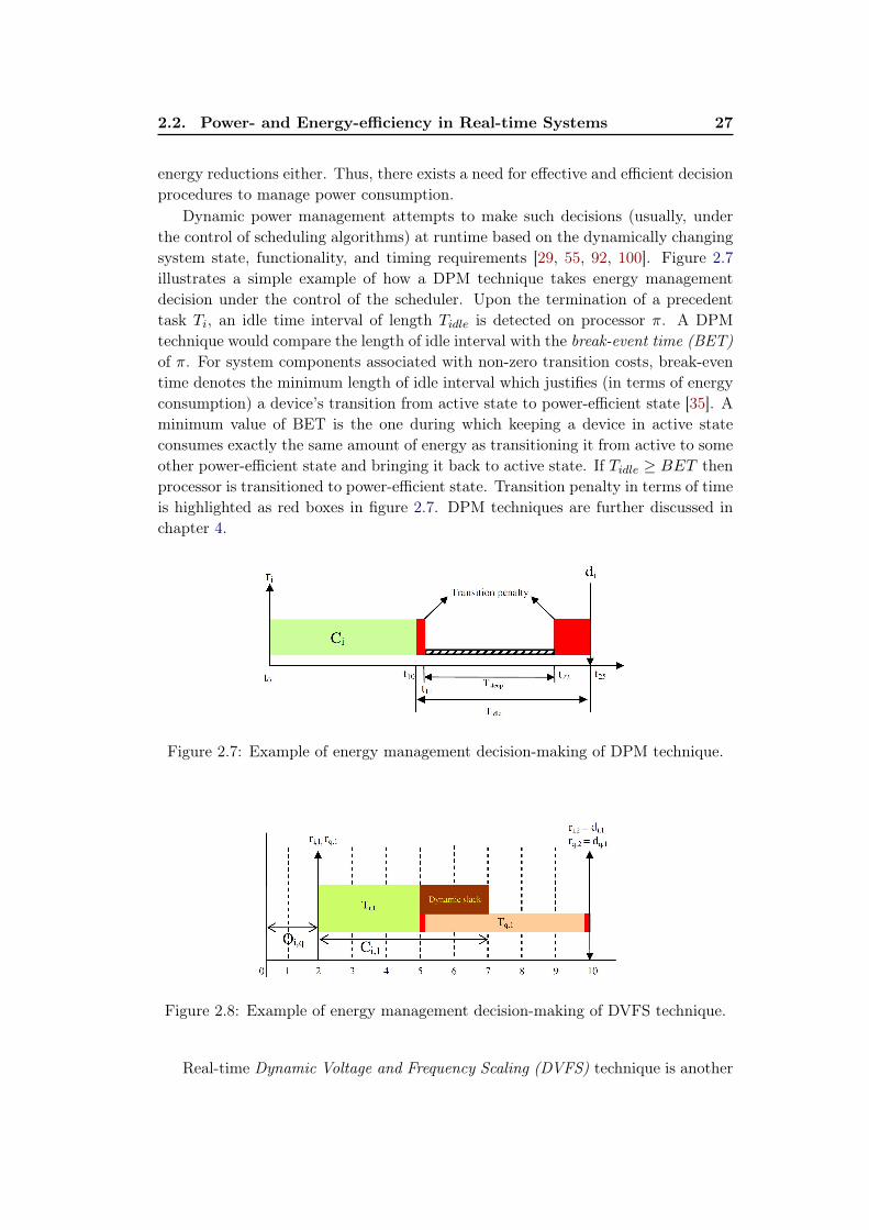
2.2. Power- and Energy-efficiency in Real-time Systems 27
energy reductions either. Thus, there exists a need for effective and efficient decisionprocedures to manage power consumption.
Dynamic power management attempts to make such decisions (usually, underthe control of scheduling algorithms) at runtime based on the dynamically changingsystem state, functionality, and timing requirements [29, 55, 92, 100]. Figure 2.7illustrates a simple example of how a DPM technique takes energy managementdecision under the control of the scheduler. Upon the termination of a precedenttask Ti, an idle time interval of length Tidle is detected on processor π. A DPMtechnique would compare the length of idle interval with the break-event time (BET)of π. For system components associated with non-zero transition costs, break-eventime denotes the minimum length of idle interval which justifies (in terms of energyconsumption) a device’s transition from active state to power-efficient state [35]. Aminimum value of BET is the one during which keeping a device in active stateconsumes exactly the same amount of energy as transitioning it from active to someother power-efficient state and bringing it back to active state. If Tidle ≥ BET thenprocessor is transitioned to power-efficient state. Transition penalty in terms of timeis highlighted as red boxes in figure 2.7. DPM techniques are further discussed inchapter 4.
Figure 2.7: Example of energy management decision-making of DPM technique.
Figure 2.8: Example of energy management decision-making of DVFS technique.
Real-time Dynamic Voltage and Frequency Scaling (DVFS) technique is another

28 Chapter 2. Background on Real-time and Energy-efficient Systems
online technique which is aimed at changing the system’s energy consumption pro-file. Real-time applications potentially exhibit variations in their actual executiontime and therefore, often finish much earlier than their estimated worst-case exe-cution time [10, 40]. DVFS technique exploits these variations in actual workloadfor dynamically adjusting the voltage and frequency of processors in order to re-duce power and energy consumption. The challenge for these techniques, however,is to preserve the feasibility of schedule and provide deadline guarantees. Thesetechniques are of particular effectiveness and interest because energy consumptionof the processor is quadratically related to the supply voltage [87, 48]. Figure 2.8illustrates a simple example of how a DVFS technique takes energy managementdecision under the control of scheduler. Figure 2.8 depicts two jobs –i.e., Ti,1 andTq,1, of different tasks being released at the same time instant with exactly thesame offset and equal deadlines. For equal deadlines, the scheduling algorithm canarbitrarily select any job in the absence of tie-breaking rules. Job Ti,1 executesfirst and finishes after executing only 3 time units which is earlier than its WCET–i.e., Ci,1=5 time units. Job Ti,1 generates 2 units of dynamic slack time (shownin red box between time instants 5 − 7). Since Tq,1 is the only successor ready jobleft, therefore, it consumes this dynamic slack to slowdown its execution on targetprocessor up to its deadline –i.e., time instant 10.
The key concern in a DVFS technique is to increase the utilization of slack timeas much as possible and to make the resultant power and energy consumption as flatas possible by adjusting the operating frequency and supply voltage of a processorunder real-time constraints. DVFS techniques can exploit not only the dynamicslack that is generated online by the workload variations, but also the worst-case(offline) slack time that occurs because of the under-utilization of processor, even ifall tasks exhibit their worst-case execution times [68]. The worst-case slack time canbe extracted from an application’s schedule before task execution. DVFS techniquesare further discussed in chapter 5.
2.3 Simulation Environment
For experimental results and evaluation of our proposed techniques in this disser-tation, we rely mainly on the simulations using a multiprocessor simulation toolcalled STORM2 (Simulation TOol for Real-time Multiprocessor scheduling) [108].This tool has been initially designed and developed to satisfy the evaluation andvalidation needs of French national project PHERMA (Parallel Heterogeneous En-ergy efficient real-time Multiprocessor Architecture) [86]. STORM is intended to: i)use as input the specifications of the hardware and software architectures togetherwith the scheduling policy; ii) simulate the system behavior using all the character-istics (task execution time, processor functioning conditions, etc.) in order to obtainthe chronological track of all the scheduling events that occurred at run time, andiii) compute various real-time metrics in order to analyze the system behavior and
2STORM has been developed at IRCCyN laboratory of the University of Nantes, France [116].
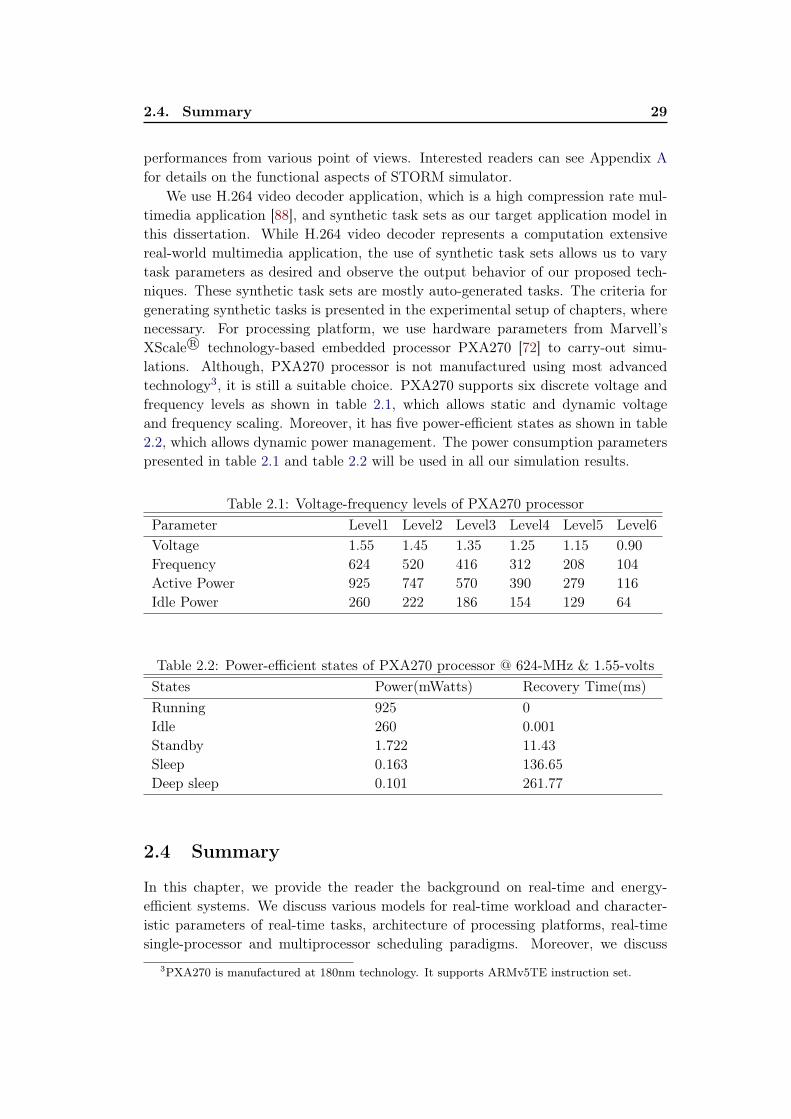
2.4. Summary 29
performances from various point of views. Interested readers can see Appendix Afor details on the functional aspects of STORM simulator.
We use H.264 video decoder application, which is a high compression rate mul-timedia application [88], and synthetic task sets as our target application model inthis dissertation. While H.264 video decoder represents a computation extensivereal-world multimedia application, the use of synthetic task sets allows us to varytask parameters as desired and observe the output behavior of our proposed tech-niques. These synthetic task sets are mostly auto-generated tasks. The criteria forgenerating synthetic tasks is presented in the experimental setup of chapters, wherenecessary. For processing platform, we use hardware parameters from Marvell’sXScale R© technology-based embedded processor PXA270 [72] to carry-out simu-lations. Although, PXA270 processor is not manufactured using most advancedtechnology3, it is still a suitable choice. PXA270 supports six discrete voltage andfrequency levels as shown in table 2.1, which allows static and dynamic voltageand frequency scaling. Moreover, it has five power-efficient states as shown in table2.2, which allows dynamic power management. The power consumption parameterspresented in table 2.1 and table 2.2 will be used in all our simulation results.
Table 2.1: Voltage-frequency levels of PXA270 processorParameter Level1 Level2 Level3 Level4 Level5 Level6Voltage 1.55 1.45 1.35 1.25 1.15 0.90Frequency 624 520 416 312 208 104Active Power 925 747 570 390 279 116Idle Power 260 222 186 154 129 64
Table 2.2: Power-efficient states of PXA270 processor @ 624-MHz & 1.55-voltsStates Power(mWatts) Recovery Time(ms)Running 925 0Idle 260 0.001Standby 1.722 11.43Sleep 0.163 136.65Deep sleep 0.101 261.77
2.4 Summary
In this chapter, we provide the reader the background on real-time and energy-efficient systems. We discuss various models for real-time workload and character-istic parameters of real-time tasks, architecture of processing platforms, real-timesingle-processor and multiprocessor scheduling paradigms. Moreover, we discuss
3PXA270 is manufactured at 180nm technology. It supports ARMv5TE instruction set.
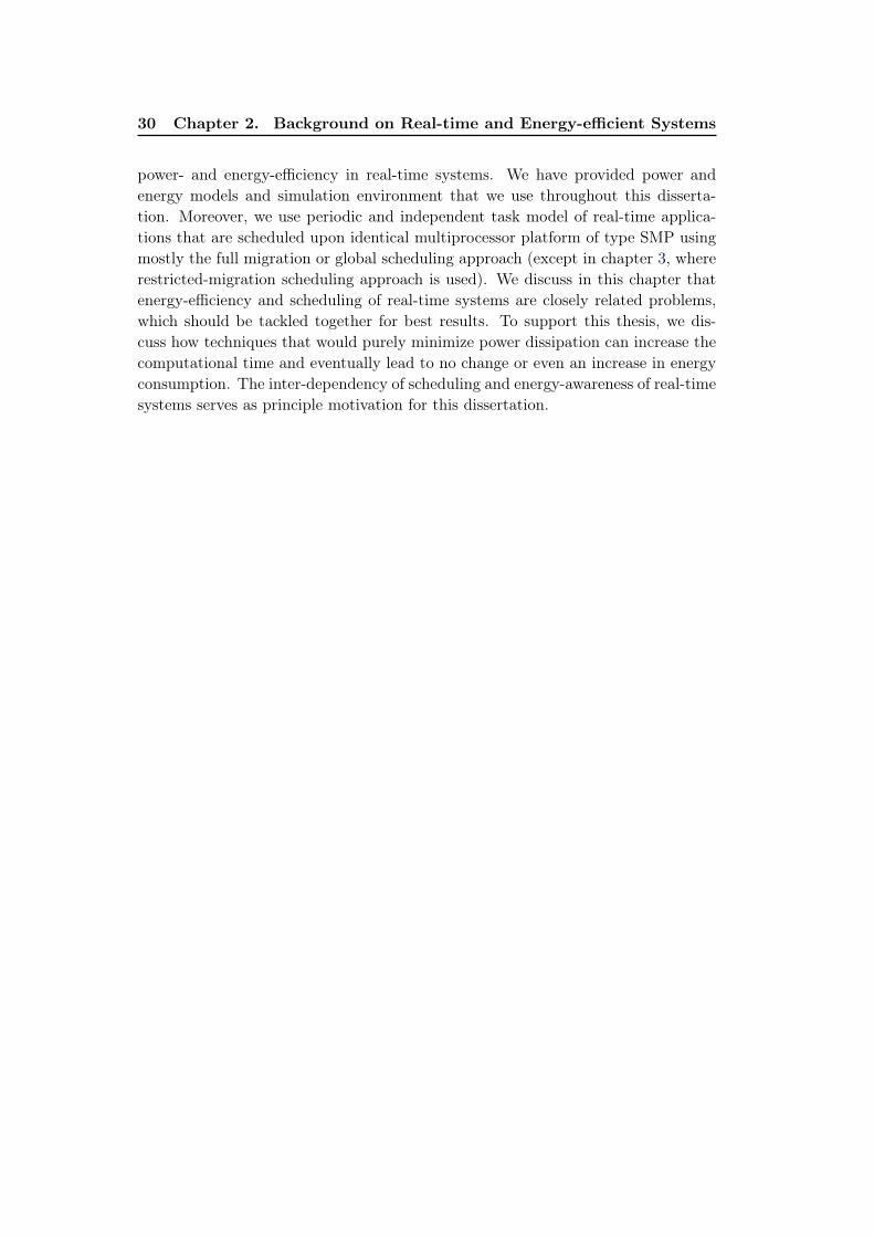
30 Chapter 2. Background on Real-time and Energy-efficient Systems
power- and energy-efficiency in real-time systems. We have provided power andenergy models and simulation environment that we use throughout this disserta-tion. Moreover, we use periodic and independent task model of real-time applica-tions that are scheduled upon identical multiprocessor platform of type SMP usingmostly the full migration or global scheduling approach (except in chapter 3, whererestricted-migration scheduling approach is used). We discuss in this chapter thatenergy-efficiency and scheduling of real-time systems are closely related problems,which should be tackled together for best results. To support this thesis, we dis-cuss how techniques that would purely minimize power dissipation can increase thecomputational time and eventually lead to no change or even an increase in energyconsumption. The inter-dependency of scheduling and energy-awareness of real-timesystems serves as principle motivation for this dissertation.
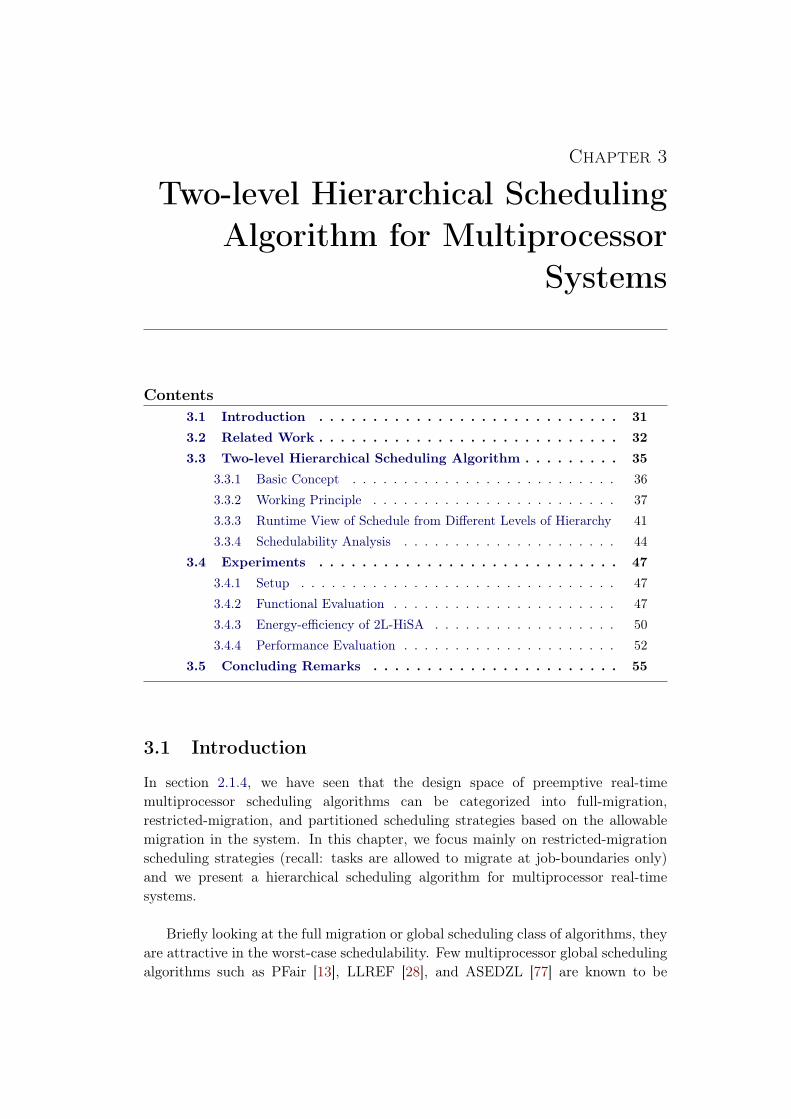
Chapter 3
Two-level Hierarchical SchedulingAlgorithm for Multiprocessor
Systems
Contents3.1 Introduction . . . . . . . . . . . . . . . . . . . . . . . . . . . . 313.2 Related Work . . . . . . . . . . . . . . . . . . . . . . . . . . . . 323.3 Two-level Hierarchical Scheduling Algorithm . . . . . . . . . 35
3.3.1 Basic Concept . . . . . . . . . . . . . . . . . . . . . . . . . . 363.3.2 Working Principle . . . . . . . . . . . . . . . . . . . . . . . . 373.3.3 Runtime View of Schedule from Different Levels of Hierarchy 413.3.4 Schedulability Analysis . . . . . . . . . . . . . . . . . . . . . 44
3.4 Experiments . . . . . . . . . . . . . . . . . . . . . . . . . . . . 473.4.1 Setup . . . . . . . . . . . . . . . . . . . . . . . . . . . . . . . 473.4.2 Functional Evaluation . . . . . . . . . . . . . . . . . . . . . . 473.4.3 Energy-efficiency of 2L-HiSA . . . . . . . . . . . . . . . . . . 503.4.4 Performance Evaluation . . . . . . . . . . . . . . . . . . . . . 52
3.5 Concluding Remarks . . . . . . . . . . . . . . . . . . . . . . . 55
3.1 Introduction
In section 2.1.4, we have seen that the design space of preemptive real-timemultiprocessor scheduling algorithms can be categorized into full-migration,restricted-migration, and partitioned scheduling strategies based on the allowablemigration in the system. In this chapter, we focus mainly on restricted-migrationscheduling strategies (recall: tasks are allowed to migrate at job-boundaries only)and we present a hierarchical scheduling algorithm for multiprocessor real-timesystems.
Briefly looking at the full migration or global scheduling class of algorithms, theyare attractive in the worst-case schedulability. Few multiprocessor global schedulingalgorithms such as PFair [13], LLREF [28], and ASEDZL [77] are known to be
32Chapter 3. Two-level Hierarchical Scheduling Algorithm for
Multiprocessor Systems
optimal. However, their scheduling overhead such as context switches and numberof migrations and preemptions in often criticized to be too large. Systems thatprohibit full migration, on the other hand, must use either partitioning or restricted-migration strategy. Between these two, the partitioning strategy is more commonlyused in current systems, reason being that partitioning-based solutions can reducethe problem of multiprocessor scheduling into multiple single-processor schedulingproblems. However, partitioning can only be used for fixed task sets. If tasks areallowed to dynamically join and leave the system, partitioning is not a viable strategybecause a task joining the system may force the whole system to be repartitioned,thus forcing tasks to migrate. Determining a new partition is a bin-packing problem,which is strong NP-hard problem [60]. Thus, repartitioning dynamic task sets incurstoo much overheads.
Restricted-migration scheduling strategies (also referred as semi-partitionedscheduling) provide a good compromise between the full migration and the par-titioning strategies [24, 63, 62]. It is flexible enough to allow dynamic tasks to jointhe system at runtime, but it does not incur large migration overheads as comparedto full-migration strategies. This strategy is particularly useful when consecutivejobs of a task do not share any data since all data passed to subsequent jobs wouldhave to be migrated at job boundaries. Furthermore, the scheduler used as top-level scheduler (if a hierarchy of schedulers exist) in restricted-migration is muchsimpler than the full-migration global scheduler. The full migration global sched-uler needs to maintain information about all active jobs in the system, whereas thetop-level scheduler in restricted migration strategy makes a single decision abouta job when it arrives and then passes the job to a local scheduler that maintainsinformation about the job from that point forward. Restricted migration strategiesoffer relatively low scheduling overhead at runtime and they are potentially veryinteresting from the point of view of system performance and energy consumption.In this chapter, we propose a scheduling algorithm based on restricted migrationstrategy, called the Two-level Hierarchical Scheduling Algorithm (2L-HiSA). Ourproposed scheduling strategy uses Earliest Deadline First (EDF) scheduling algo-rithm in a hierarchical fashion at both top-level and local-level scheduler. Authors in[8] highlight that a significant disparity in schedulability exists between EDF-basedscheduling algorithms and existing global optimal scheduling algorithms. This is un-fortunate because EDF-based algorithms entail lower scheduling and task-migrationoverheads. In this work, we show that by using multiple instances of EDF schedul-ing algorithm at different levels of hierarchy, the wort-case schedulability bound ofEDF can be improved.
3.2 Related Work
Some novel and promising techniques in the category of restricted-migration schedul-ing have been proposed very recently with the main objective of reducing the runtimeoverhead of scheduler and improving the schedulability and system utilization bound
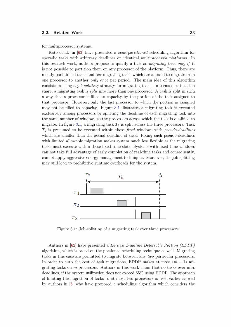
3.2. Related Work 33
for multiprocessor systems.Kato et al. in [63] have presented a semi-partitioned scheduling algorithm for
sporadic tasks with arbitrary deadlines on identical multiprocessor platforms. Inthis research work, authors propose to qualify a task as migrating task only if itis not possible to partition them on any processor of the platform. Thus, there aremostly partitioned tasks and few migrating tasks which are allowed to migrate fromone processor to another only once per period. The main idea of this algorithmconsists in using a job-splitting strategy for migrating tasks. In terms of utilizationshare, a migrating task is split into more than one processor. A task is split in sucha way that a processor is filled to capacity by the portion of the task assigned tothat processor. However, only the last processor to which the portion is assignedmay not be filled to capacity. Figure 3.1 illustrates a migrating task is executedexclusively among processors by splitting the deadline of each migrating task intothe same number of windows as the processors across which the task is qualified tomigrate. In figure 3.1, a migrating task Tk is split across the three processors. TaskTk is presumed to be executed within these fixed windows with pseudo-deadlineswhich are smaller than the actual deadline of task. Fixing such pseudo-deadlineswith limited allowable migration makes system much less flexible as the migratingtasks must execute within these fixed time slots. Systems with fixed time windowscan not take full advantage of early completion of real-time tasks and consequently,cannot apply aggressive energy management techniques. Moreover, the job-splittingmay still lead to prohibitive runtime overheads for the system.
Figure 3.1: Job-splitting of a migrating task over three processors.
Authors in [62] have presented a Earliest Deadline Deferrable Portion (EDDP)algorithm, which is based on the portioned scheduling technique as well. Migratingtasks in this case are permitted to migrate between any two particular processors.In order to curb the cost of task migrations, EDDP makes at most (m − 1) mi-grating tasks on m-processors. Authors in this work claim that no tasks ever missdeadlines, if the system utilization does not exceed 65% using EDDP. The approachof limiting the migration of tasks to at most two processors is used earlier as wellby authors in [8] who have proposed a scheduling algorithm which considers the
34Chapter 3. Two-level Hierarchical Scheduling Algorithm for
Multiprocessor Systems
trade-off between system utilization and number of preemptions for recurring tasksystems. The migration overhead is relaxed in this approach compared to the otheroptimal multiprocessor algorithms by limiting the number of migrating tasks. Thealgorithm trades an achievable system utilization with the cost of preemptions byadjusting a parameter k, where 2 ≤ k ≤ m. For k < m, the achievable utilizationis claimed to be k/(k + 1). For k = m, on the other hand, it is 100%, thereby theirproposed algorithm performs optimally. Based on the work of [8, 62, 63], authorsin [38] have also propose a semi-partitioned hard real-time scheduling approach forsporadic deadline-constrained tasks upon identical multiprocessor platforms. In thiswork, migration of jobs is prohibited except that two subsequent jobs of a task canbe assigned to different processors by applying a periodic strategy. This techniquecomprises two steps: an assigning phase and a scheduling phase. The assigningphase is somewhat similar to that of [63]. That is, if it is not possible to partitiona task without violating schedulability guarantees then the concerned task is classi-fied as migrating task. Authors propose to distribute jobs of migrating task amongseveral processors using a multi-frame tasking approach with a predefined periodicsequence of the occurrence of jobs on various processors. This predefined sequenceof jobs repeats itself cyclically at runtime upon the selected processors. The limita-tion of this approach is the assumption that the number of frames of each migratingtask over multiple processors must be available beforehand to provide schedulabilityanalysis. Moreover, in [38] and [62], the schedulability bound is 65% which is stillnot considerably large w.r.t. previously proposed partitioned scheduling algorithmsoffering 50% utilization bound in worst-case.
Calandrino et al. in [24] have proposed a hybrid scheduling approach for soft real-time tasks on large-scale multiprocessor platforms with hierarchical shared caches.In this approach, a multiprocessor platform is partitioned into clusters, tasks arestatically assigned to these clusters (rather than individual processors), and sched-uled within each cluster using the preemptive global EDF scheduling algorithm. Alltasks are allowed to migrate within a cluster but not across clusters. Authors in thiswork demonstrate that, by partitioning the system into clusters instead of individualcores, bin-packing limitations can be alleviated by effectively increasing bin-sizes incomparison to item-sizes. However, this work still uses a common global schedulerat cluster-level which is equivalent to breaking a larger multiprocessor schedulingproblem into multiple smaller multiprocessor scheduling problems. Moreover, thesolution is limited to soft real-time applications. In contrast to [24], authors in[114] have proposed a two-level scheduling scheme, which uses the idea of sporadicservers. In this approach, first an application is partitioned into parallel tasks asmuch as possible. Then the parallel tasks are dispatched to different processors, soas to execute in parallel. On each processor, real-time tasks run concurrently withnon real-time tasks. At the top level, a sporadic server is assigned to each schedulingpolicy while at the bottom level, a Rate-Monotonic (RM) scheduler is adopted tomaintain and schedule the top-level sporadic servers. While this research work usesa two-level hierarchy of schedulers, only soft real-time applications are consideredfor scheduling.
3.3. Two-level Hierarchical Scheduling Algorithm 35
Our proposed two-level hierarchical scheduling algorithm statically partitions asmuch tasks as possible to processors, which is somewhat similar to that of [62].However, neither the number of migrating tasks nor the number of migrations permigrating task is limited in our approach, which is contrary to that of [24], [38], and[62]. Moreover, unlike in [62], 2L-HiSA does not fix time slots for migrating tasks.Rather it reserves a portion of processor time on each processor (in proportion to itsunder-utilization) for migrating tasks and this portion of time can be dynamicallyrelocated by local-level scheduler within a specified period to allow the execution ofstatically partitioned tasks. This dynamic relocation of reserved time for migratingtasks improves system flexibility both at design-time and runtime. In section 3.3,we provide the 2L-HiSA scheduling algorithm in detail.
3.3 Two-level Hierarchical Scheduling Algorithm
The 2L-HiSA scheduling algorithm uses multiple instances of single-processor opti-mal EDF scheduling algorithm in a hierarchical fashion at two levels: an instance attop-level scheduler and an instance at local-level scheduler on every processor of theplatform. Since EDF is an optimal single-processor scheduling algorithm, therefore,in order to determine whether the given task set is EDF-schedulable, it suffices todetermine whether this task set is feasible on the single-processor systems. Unfortu-nately, it has been shown in [34, 52] that there are no optimal job-level fixed-priorityscheduling algorithms for multiprocessors. Since EDF falls in this category, there-fore, determining whether a given task set is feasible on a multiprocessor system willnot tell us whether the same task set is EDF-schedulable on the same system as well.Baruah, et al. proved in [13] that there exists a job-level dynamic-priority schedulingalgorithm, referred as PFair, which is optimal for periodic task sets on multipro-cessors. Srinivasan and Anderson later showed in [106] that this algorithm can bemodified to be optimal for sporadic task sets as well. However, these results do notapply on EDF because they use a job-level dynamic-priority algorithm. On the is-sue of determining EDF-schedulability, authors in [5] have provided schedulable uti-lization bounds for job-level fixed-priority scheduling algorithms for full-migration,restricted-migration, and partitioned scheduling strategies. EDF, being a job-levelfixed-priority algorithm, has schedulable utilization bounds of m2
2m−1 ≤ Usum ≤m+12
for full-migration strategies, Usum = βm+1β+1 (β =
⌊1α
⌋) for no-migration strategies,
and m − α(m − 1) ≤ Usum ≤ m+12 or otherwise for restricted-migration strate-
gies, respectively. Here, the term α represents a cap on individual task utilizations.Note that, if such a cap is not exploited, then the upper bound on schedulableutilization is approximately m
2 or lower. Authors in [7] state that, for a periodictask set with implicit deadlines, the schedulable utilization under EDF or any otherstatic-priority multiprocessor scheduling algorithm –partitioned or global– can notbe higher than m+1
2 for m processors. Clearly, under this schedulability bound, amultiprocessor platform suffers heavily from under-utilization (i.e., by a factor ofm−12 ). For instance, in a system composed of three processors (m = 3), platform re-
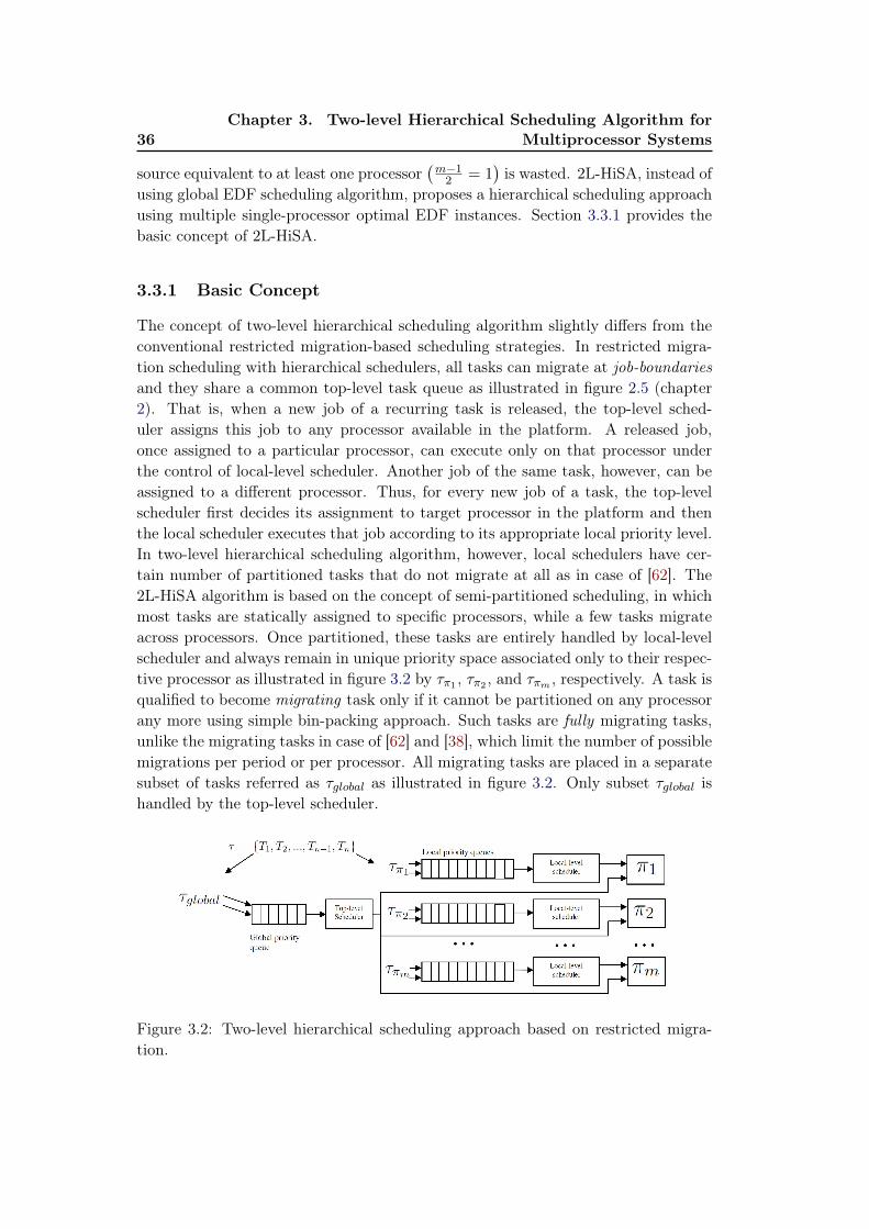
36Chapter 3. Two-level Hierarchical Scheduling Algorithm for
Multiprocessor Systems
source equivalent to at least one processor(m−12 = 1
)is wasted. 2L-HiSA, instead of
using global EDF scheduling algorithm, proposes a hierarchical scheduling approachusing multiple single-processor optimal EDF instances. Section 3.3.1 provides thebasic concept of 2L-HiSA.
3.3.1 Basic Concept
The concept of two-level hierarchical scheduling algorithm slightly differs from theconventional restricted migration-based scheduling strategies. In restricted migra-tion scheduling with hierarchical schedulers, all tasks can migrate at job-boundariesand they share a common top-level task queue as illustrated in figure 2.5 (chapter2). That is, when a new job of a recurring task is released, the top-level sched-uler assigns this job to any processor available in the platform. A released job,once assigned to a particular processor, can execute only on that processor underthe control of local-level scheduler. Another job of the same task, however, can beassigned to a different processor. Thus, for every new job of a task, the top-levelscheduler first decides its assignment to target processor in the platform and thenthe local scheduler executes that job according to its appropriate local priority level.In two-level hierarchical scheduling algorithm, however, local schedulers have cer-tain number of partitioned tasks that do not migrate at all as in case of [62]. The2L-HiSA algorithm is based on the concept of semi-partitioned scheduling, in whichmost tasks are statically assigned to specific processors, while a few tasks migrateacross processors. Once partitioned, these tasks are entirely handled by local-levelscheduler and always remain in unique priority space associated only to their respec-tive processor as illustrated in figure 3.2 by τπ1 , τπ2 , and τπm , respectively. A task isqualified to become migrating task only if it cannot be partitioned on any processorany more using simple bin-packing approach. Such tasks are fully migrating tasks,unlike the migrating tasks in case of [62] and [38], which limit the number of possiblemigrations per period or per processor. All migrating tasks are placed in a separatesubset of tasks referred as τglobal as illustrated in figure 3.2. Only subset τglobal ishandled by the top-level scheduler.
Figure 3.2: Two-level hierarchical scheduling approach based on restricted migra-tion.
3.3. Two-level Hierarchical Scheduling Algorithm 37
Top-level scheduler assigns tasks from τglobal to processors at runtime withinsuitable time slots. These suitable time slots are actually the portion of processortime that is determined on every processor based on its under-utilization (if any).Section 3.3.2 gives more details on the procedure for determining the size, periodic-ity, and priority of these time slots. However, it is worth mentioning here that thesetime slots occur explicitly on processors in an m-processor platform –i.e., they do notoccur in parallel. Moreover, these time slots are not fixed (like in case of [62]) andoccur dynamically within the specified period. Due to the NP-hardness of the par-titioning problem, processors in a multiprocessor platform are often under-utilizedwith a significant margin in a post-partitioned scenario.
3.3.2 Working Principle
In this section, we provide the main steps of our proposed algorithm. 2L-HiSA, asmentioned earlier, is based on the concept of restricted migration scheduling andconsists of two phases:
1. The task-partitioning phase: In this phase, each non-migrating task is (of-fline/statically) assigned to a specific processor by following the bin-packingapproach.
2. The processor-grouping phase: This is a post-partitioning phase in which,processors are grouped together based on their workload characteristics.
3.3.2.1 The task-partitioning phase
Let us consider that a real-time task set τ containing at most n tasks such thatτ = {T1, Ti, ...Tn−1, Tn}, has to be scheduled on an identical multiprocessor plat-form composed of m processors. The task set is considered feasible a priori -i.e.,Usum(τ) =
∑ni=1 ui ≤ m. In the first step of our algorithm, each task Ti is stati-
cally assigned to a particular processor πk by following the bin-packing approach,as long as the task does not cause violation of schedulability of tasks being already
partitioned upon processor πk –i.e., Usum(τπk)def= (L>0)
DBF(τπk ,L)L ≤ 1, where tasks
being partitioned on a particular processor πk are denoted by τπk , L refers to inter-val length, and DBF refers to the classical Demand Bound Function [38, 77]. Notethat the task-partitioning can be performed using any suitable partitioning strategy.Algorithm 1 illustrates the task partitioning phase. In the first step, before parti-tioning any task to processors, the utilization of each processor πk is initialized tozero –i.e., Uπk = 0 (lines 1−5). In the second step, each task is tested for partition-ing on m processors of the platform according to the condition mentioned earlier(lines 6− 14). If, for any task Ti, Usum(τπk) > 1 –i.e., it can not be partitioned onπk (∀k, 1 ≤ k ≤ m), then this task is classified as migrating task and assigned toτglob subset of tasks (lines 1− 18).
For a feasible task set τ , often it is not possible to partition all tasks due to theNP-hardness of partitioning problem. Thus, in our algorithm, a given τ is divided

38Chapter 3. Two-level Hierarchical Scheduling Algorithm for
Multiprocessor Systems
Algorithm 1 Offline task partitioning to processors1: n← number of tasks in τ2: m← number of processors in Π
3: for k = 1...m do4: Uπk ← 0;5: for i = 1...n do6: for k = 1...m do7: if Uπk + ui ≤ 1 then8: assign Ti to πk;9: Uπk=Uπk + ui;
10: remove Ti from τ ;11: break;12: if size(τ) 6= 0 then13: assign all remaining tasks to τglob;
into two subsets of tasks such that Usum(τpart) + Usum(τglob) = Usum(τ) ≤ m. In apost-partitioned scenario, we can calculate the aggregate utilization of tasks beingstatically partitioned on (or assigned to) every processor (πk) individually usingequation 3.1. Here, np refers to the total number of tasks being partitioned on aparticular processor πk.
Uπk(τπk) =
np∑i=1
CiPi
(∀i, 1 ≤ i ≤ np, ∀Ti ∈ τpart) (3.1)
From equation 3.1, we can compute the under-utilization present on every pro-cessor πk using equation 3.2. Let the under-utilization present on any processor πkbe referred as U ′
πk.
U′
πk(τπk) = 1−
np∑i=1
CiPi
(∀i, 1 ≤ i ≤ np, ∀Ti ∈ τpart) (3.2)
3.3.2.2 The processor-grouping phase
In the second step, we group processors of the platform Π in such a way that thecumulated under-utilization on all processors within a group is not greater than one–i.e.,
∑U
′πk≤ 1. In section 3.3.1, it is stated that a portion of processor time is
reserved on every processor in proportion to its U ′πk
to which, the top-level schedulercould exploit for scheduling tasks from τglob. Moreover, these portions of processortime must appear explicitly. Now, if the cumulated under-utilization of processorswill be more than one, then the computation power equivalent to more than oneprocessor will be free within the system. This under-utilization will cause idle timeintervals to appear in parallel on certain processors which is not desirable. Thus,grouping processors such that the sum of under-utilization on all processors withina group is not greater than one allows to have a cumulated (but still fragmented)computation power equivalent to at most one processor free within each group.This condition helps avoiding parallelism of the idle time intervals that would occur
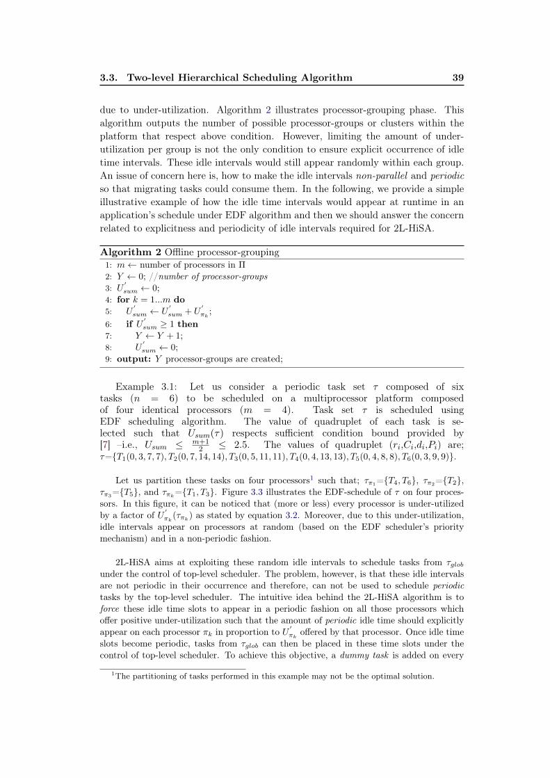
3.3. Two-level Hierarchical Scheduling Algorithm 39
due to under-utilization. Algorithm 2 illustrates processor-grouping phase. Thisalgorithm outputs the number of possible processor-groups or clusters within theplatform that respect above condition. However, limiting the amount of under-utilization per group is not the only condition to ensure explicit occurrence of idletime intervals. These idle intervals would still appear randomly within each group.An issue of concern here is, how to make the idle intervals non-parallel and periodicso that migrating tasks could consume them. In the following, we provide a simpleillustrative example of how the idle time intervals would appear at runtime in anapplication’s schedule under EDF algorithm and then we should answer the concernrelated to explicitness and periodicity of idle intervals required for 2L-HiSA.
Algorithm 2 Offline processor-grouping1: m← number of processors in Π
2: Y ← 0; //number of processor-groups3: U
′
sum ← 0;4: for k = 1...m do5: U
′
sum ← U′
sum + U′
πk;
6: if U′
sum ≥ 1 then7: Y ← Y + 1;8: U
′
sum ← 0;9: output: Y processor-groups are created;
Example 3.1: Let us consider a periodic task set τ composed of sixtasks (n = 6) to be scheduled on a multiprocessor platform composedof four identical processors (m = 4). Task set τ is scheduled usingEDF scheduling algorithm. The value of quadruplet of each task is se-lected such that Usum(τ) respects sufficient condition bound provided by[7] –i.e., Usum ≤ m+1
2 ≤ 2.5. The values of quadruplet (ri,Ci,di,Pi) are;τ={T1(0, 3, 7, 7), T2(0, 7, 14, 14), T3(0, 5, 11, 11), T4(0, 4, 13, 13), T5(0, 4, 8, 8), T6(0, 3, 9, 9)}.
Let us partition these tasks on four processors1 such that; τπ1={T4, T6}, τπ2
={T2},τπ3
={T5}, and τπk={T1, T3}. Figure 3.3 illustrates the EDF-schedule of τ on four proces-sors. In this figure, it can be noticed that (more or less) every processor is under-utilizedby a factor of U
′
πk(τπk) as stated by equation 3.2. Moreover, due to this under-utilization,
idle intervals appear on processors at random (based on the EDF scheduler’s prioritymechanism) and in a non-periodic fashion.
2L-HiSA aims at exploiting these random idle intervals to schedule tasks from τglobunder the control of top-level scheduler. The problem, however, is that these idle intervalsare not periodic in their occurrence and therefore, can not be used to schedule periodictasks by the top-level scheduler. The intuitive idea behind the 2L-HiSA algorithm is toforce these idle time slots to appear in a periodic fashion on all those processors whichoffer positive under-utilization such that the amount of periodic idle time should explicitlyappear on each processor πk in proportion to U
′
πkoffered by that processor. Once idle time
slots become periodic, tasks from τglob can then be placed in these time slots under thecontrol of top-level scheduler. To achieve this objective, a dummy task is added on every
1The partitioning of tasks performed in this example may not be the optimal solution.
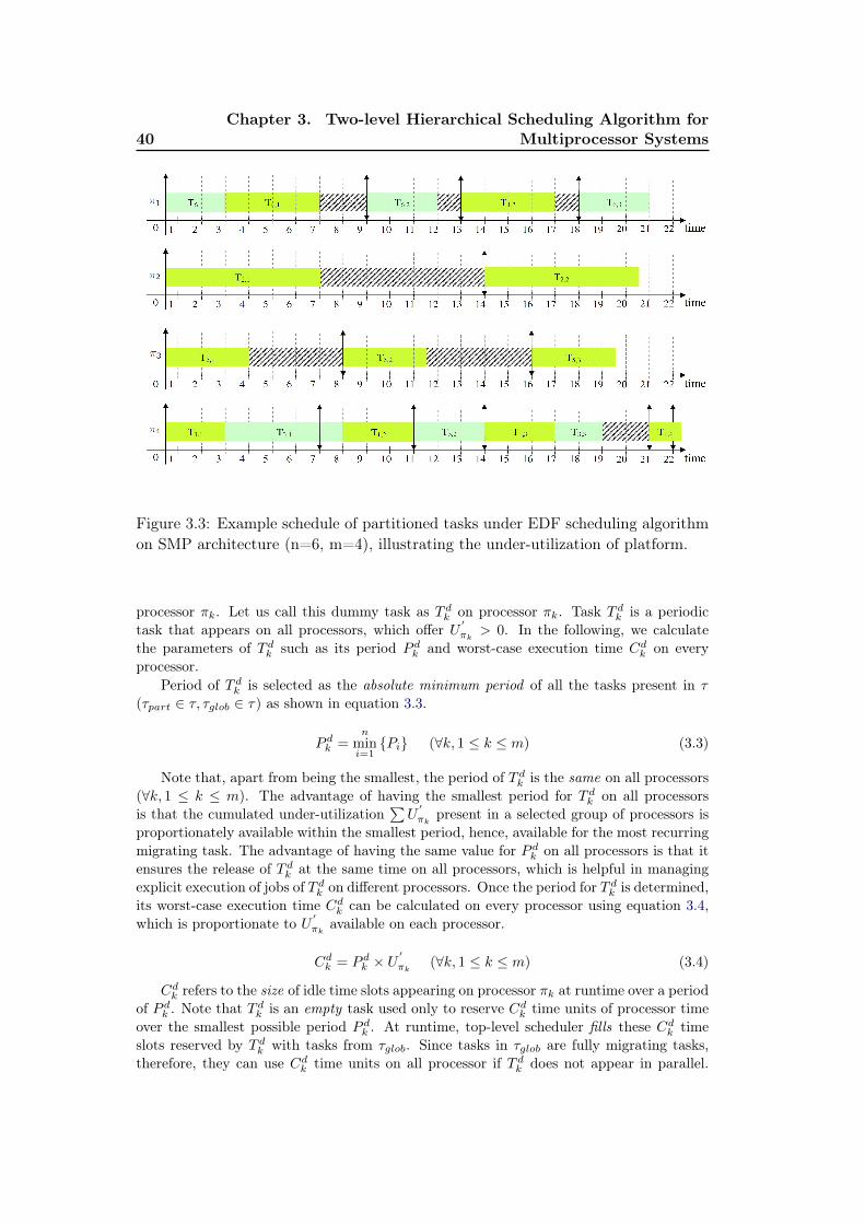
40Chapter 3. Two-level Hierarchical Scheduling Algorithm for
Multiprocessor Systems
Figure 3.3: Example schedule of partitioned tasks under EDF scheduling algorithmon SMP architecture (n=6, m=4), illustrating the under-utilization of platform.
processor πk. Let us call this dummy task as T dk on processor πk. Task T dk is a periodictask that appears on all processors, which offer U
′
πk> 0. In the following, we calculate
the parameters of T dk such as its period P dk and worst-case execution time Cdk on everyprocessor.
Period of T dk is selected as the absolute minimum period of all the tasks present in τ
(τpart ∈ τ, τglob ∈ τ) as shown in equation 3.3.
P dk =n
mini=1{Pi} (∀k, 1 ≤ k ≤ m) (3.3)
Note that, apart from being the smallest, the period of T dk is the same on all processors(∀k, 1 ≤ k ≤ m). The advantage of having the smallest period for T dk on all processorsis that the cumulated under-utilization
∑U
′
πkpresent in a selected group of processors is
proportionately available within the smallest period, hence, available for the most recurringmigrating task. The advantage of having the same value for P dk on all processors is that itensures the release of T dk at the same time on all processors, which is helpful in managingexplicit execution of jobs of T dk on different processors. Once the period for T dk is determined,its worst-case execution time Cdk can be calculated on every processor using equation 3.4,which is proportionate to U
′
πkavailable on each processor.
Cdk = P dk × U′
πk(∀k, 1 ≤ k ≤ m) (3.4)
Cdk refers to the size of idle time slots appearing on processor πk at runtime over a periodof P dk . Note that T dk is an empty task used only to reserve Cdk time units of processor timeover the smallest possible period P dk . At runtime, top-level scheduler fills these Cdk timeslots reserved by T dk with tasks from τglob. Since tasks in τglob are fully migrating tasks,therefore, they can use Cdk time units on all processor if T dk does not appear in parallel.
3.3. Two-level Hierarchical Scheduling Algorithm 41
Thus, one of the design consideration of 2L-HiSA is to make sure that T dk is non-parallel orexplicit on processors within a group over the interval lengths of P dk .
Since T dk has the same period (P dk ) on every processor, therefore, it releases at the sametime on all processors. Moreover, making P dk being the smallest period within the taskset τ also makes T dk the highest priority task on every processor under EDF schedulingalgorithm. Thus, to ensure explicit execution of T dk , the 2L-HiSA algorithm performs apriority exchange of T dk with highest priority local task on all those processors within agroup on which T dk is not selected for execution at time instant t. This priority exchange isnon-blocking from the platform resources point of view –i.e., exchanging the priority of T dkwith local/partitioned task on a processor πk does not cause processor πk to become idle orblocked as long as statically partitioned ready tasks exist. We illustrate this concept withan example in the following.
Let us consider a multiprocessor platform with three processors belonging to the samegroup. Each processor has a dummy task T dk assigned to it. At time instant t = 0, T dkis released on all three processors simultaneously. If T d1 , which is the dummy task onprocessor π1, is assigned on π1 as illustrated in figure 3.4, then the local schedulers on π2and π3 exchange the priority of T d2 and T d3 with local tasks, respectively, to give higherpriority to statically partitioned ready task that is having the highest priority (if any).Upon termination of T d1 on π1 at time instant t = 1, remaining two processors π2 and π3revert the priority of their respective dummy tasks T d2 and T d3 , respectively, to allow themto compete for priority at local scheduler’s level. Since, at most one local scheduler canassign T dk on a processor at any time to ensure explicit execution of jobs of T dk , therefore,the other local schedulers exchange priority of their respective T dk again to allow partitionedtasks to execute. In this example, after T d1 is terminated on π1, local scheduler on π2 assignsT d2 and local scheduler on π3 again exchanges the priority of T d3 to let the partitioned tasksrun. Finally, at time instant t = 2, local scheduler on π3 assigns T d3 for execution. At timet = 3, T d1 , T d2 , and T d3 are released again and compete for assignment on their respectiveprocessors. Note that T dk has no specific order of occurrence –i.e., fixed time slot that canbe defined a priori on different processors. A newly released job of T dk has to, first, competefor the priority among locally partitioned tasks and then compete for priority among T dkpresent on other processors within a group. Failure to obtain highest priority at any ofthe two levels cause a priority exchange for concerned task. This makes the portion ofprocessors’ time reserved for τglob to appear in a sequential fashion over P dk within a groupof processors. The priority exchange for T dk on the same processor can be performed up tothe time instant when laxity of T dk becomes zero.
3.3.3 Runtime View of Schedule from Different Levels of Hierarchy
In this section, we provide the reader the view-points of both top-level and local-levelschedulers under the 2L-HiSA algorithm.
3.3.3.1 Local-level Scheduler
From the earlier discussion, we know that single-processor optimal EDF scheduling algo-rithm is used as local scheduler on every processor to schedule statically partitioned tasks.Along with tasks being partitioned on each processor πk –i.e., τπk , there is a dummy taskT dk assigned on each processor that has an execution requirement of Cdk , which is exactlyequal to the amount of U
′
πkavailable on πk –i.e., U
′
πk= 1−Uπk =
CdkPdk
. Thus, the worst-case
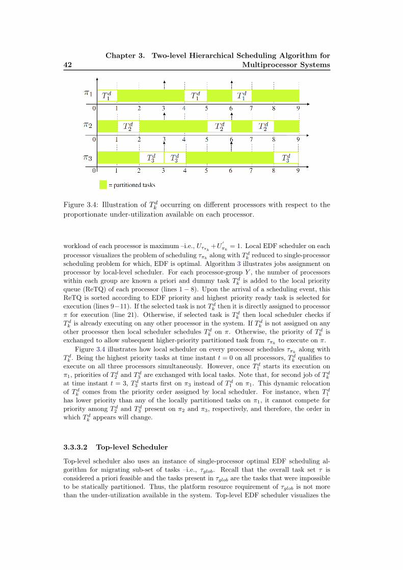
42Chapter 3. Two-level Hierarchical Scheduling Algorithm for
Multiprocessor Systems
Figure 3.4: Illustration of T dk occurring on different processors with respect to theproportionate under-utilization available on each processor.
workload of each processor is maximum –i.e., Uτπk +U′
πk= 1. Local EDF scheduler on each
processor visualizes the problem of scheduling τπk along with T dk reduced to single-processorscheduling problem for which, EDF is optimal. Algorithm 3 illustrates jobs assignment onprocessor by local-level scheduler. For each processor-group Y , the number of processorswithin each group are known a priori and dummy task T dk is added to the local priorityqueue (ReTQ) of each processor (lines 1− 8). Upon the arrival of a scheduling event, thisReTQ is sorted according to EDF priority and highest priority ready task is selected forexecution (lines 9−11). If the selected task is not T dk then it is directly assigned to processorπ for execution (line 21). Otherwise, if selected task is T dk then local scheduler checks ifT dk is already executing on any other processor in the system. If T dk is not assigned on anyother processor then local scheduler schedules T dk on π. Otherwise, the priority of T dk isexchanged to allow subsequent higher-priority partitioned task from τπk to execute on π.
Figure 3.4 illustrates how local scheduler on every processor schedules τπk along withT dk . Being the highest priority tasks at time instant t = 0 on all processors, T dk qualifies toexecute on all three processors simultaneously. However, once T d1 starts its execution onπ1, priorities of T d2 and T d3 are exchanged with local tasks. Note that, for second job of T dkat time instant t = 3, T d3 starts first on π3 instead of T d1 on π1. This dynamic relocationof T dk comes from the priority order assigned by local scheduler. For instance, when T d1has lower priority than any of the locally partitioned tasks on π1, it cannot compete forpriority among T d2 and T d3 present on π2 and π3, respectively, and therefore, the order inwhich T dk appears will change.
3.3.3.2 Top-level Scheduler
Top-level scheduler also uses an instance of single-processor optimal EDF scheduling al-gorithm for migrating sub-set of tasks –i.e., τglob. Recall that the overall task set τ isconsidered a priori feasible and the tasks present in τglob are the tasks that were impossibleto be statically partitioned. Thus, the platform resource requirement of τglob is not morethan the under-utilization available in the system. Top-level EDF scheduler visualizes the
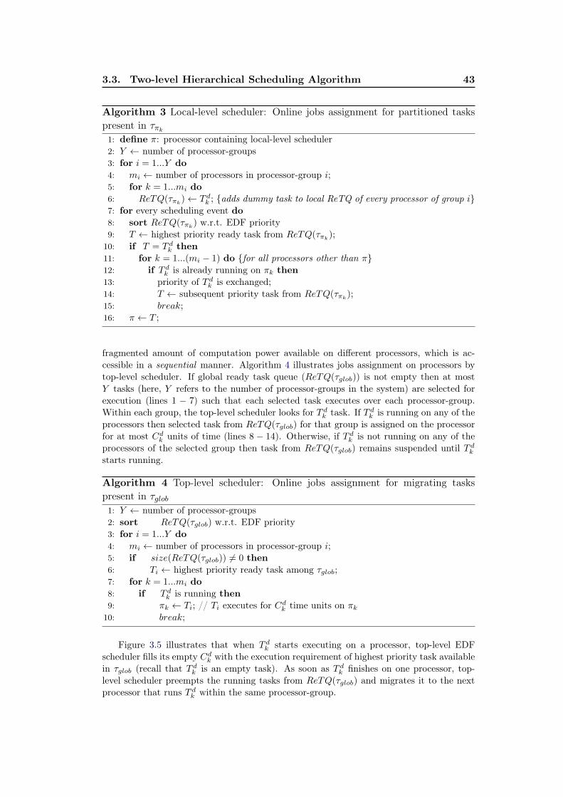
3.3. Two-level Hierarchical Scheduling Algorithm 43
Algorithm 3 Local-level scheduler: Online jobs assignment for partitioned taskspresent in τπk1: define π: processor containing local-level scheduler2: Y ← number of processor-groups3: for i = 1...Y do4: mi ← number of processors in processor-group i;5: for k = 1...mi do6: ReTQ(τπk)← T dk ; {adds dummy task to local ReTQ of every processor of group i}7: for every scheduling event do8: sort ReTQ(τπk) w.r.t. EDF priority9: T ← highest priority ready task from ReTQ(τπk);
10: if T = T dk then11: for k = 1...(mi − 1) do {for all processors other than π}12: if T dk is already running on πk then13: priority of T dk is exchanged;14: T ← subsequent priority task from ReTQ(τπk);15: break;16: π ← T ;
fragmented amount of computation power available on different processors, which is ac-cessible in a sequential manner. Algorithm 4 illustrates jobs assignment on processors bytop-level scheduler. If global ready task queue (ReTQ(τglob)) is not empty then at mostY tasks (here, Y refers to the number of processor-groups in the system) are selected forexecution (lines 1 − 7) such that each selected task executes over each processor-group.Within each group, the top-level scheduler looks for T dk task. If T dk is running on any of theprocessors then selected task from ReTQ(τglob) for that group is assigned on the processorfor at most Cdk units of time (lines 8 − 14). Otherwise, if T dk is not running on any of theprocessors of the selected group then task from ReTQ(τglob) remains suspended until T dkstarts running.
Algorithm 4 Top-level scheduler: Online jobs assignment for migrating taskspresent in τglob1: Y ← number of processor-groups2: sort ReTQ(τglob) w.r.t. EDF priority3: for i = 1...Y do4: mi ← number of processors in processor-group i;5: if size(ReTQ(τglob)) 6= 0 then6: Ti ← highest priority ready task among τglob;7: for k = 1...mi do8: if T dk is running then9: πk ← Ti; // Ti executes for Cdk time units on πk
10: break;
Figure 3.5 illustrates that when T dk starts executing on a processor, top-level EDFscheduler fills its empty Cdk with the execution requirement of highest priority task availablein τglob (recall that T dk is an empty task). As soon as T dk finishes on one processor, top-level scheduler preempts the running tasks from ReTQ(τglob) and migrates it to the nextprocessor that runs T dk within the same processor-group.
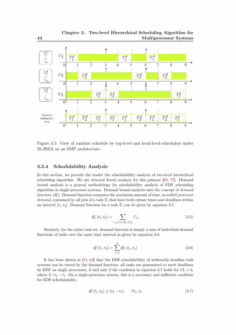
44Chapter 3. Two-level Hierarchical Scheduling Algorithm for
Multiprocessor Systems
Figure 3.5: View of runtime schedule by top-level and local-level schedulers under2L-HiSA on an SMP architecture.
3.3.4 Schedulability Analysis
In this section, we provide the reader the schedulability analysis of two-level hierarchicalscheduling algorithm. We use demand bound analysis for this purpose [63, 77]. Demandbound analysis is a general methodology for schedulability analysis of EDF schedulingalgorithm in single-processor systems. Demand bound analysis uses the concept of demandfunction (df). Demand function computes the maximum amount of time, so-called processordemand, consumed by all jobs of a task Ti that have both release times and deadlines withinan interval [t1, t2]. Demand function for a task Ti can be given by equation 3.5.
dfi (t1, t2) =∑
rij≥t1,dij≤t2
Cij (3.5)
Similarly, for the entire task set, demand function is simply a sum of individual demandfunctions of tasks over the same time interval as given by equation 3.6.
df (t1, t2) =
n∑i=1
dfi (t1, t2) (3.6)
It has been shown in [15, 63] that the EDF-schedulability of arbitrarily-deadline tasksystems can be tested by the demand function: all tasks are guaranteed to meet deadlinesby EDF on single processors, if and only if the condition in equation 3.7 holds for ∀L > 0,where L=t2 − t1. On a single-processor system, this is a necessary and sufficient conditionfor EDF-schedulability.
df (t1, t2) ≤ (t2 − t1) ∀t1, t2 (3.7)
3.3. Two-level Hierarchical Scheduling Algorithm 45
We divide the schedulability analysis of 2L-HiSA into two parts. In the first part, weanalyze the EDF-schedulability of migrating tasks and in second part, we analyze EDF-schedulability of partitioned tasks.
3.3.4.1 Schedulability of migrating tasks
As discussed earlier in section 3.3.2, subset of migrating tasks can not have an aggregateutilization (τglob) more than the under-utilization available in the system (Usum(τglob) ≤∑mk=1 U
′
πk). We have illustrated in figure 3.5 that this under-utilization is proportionately
fragmented over different processors of the system and the computation power not morethan the equivalent of one processor is freely available within each group. Top-level EDFscheduler, thus, has this fragmented computation power (more than or equal to the cu-mulated execution requirement of migrating tasks) available in the system to which, it canaccess in a sequential manner thanks to the explicit occurrence of T dk (see figure 3.5). More-over, T dk is the most frequently occurring task on every processor (i.e., it recurs over thesmallest period). Thus, migrating tasks always find the portion of processor time reservedfor them, which is sufficient w.r.t. their execution requirement. Partitioned tasks, on theother hand, find the remaining non-reserved time units to execute.
3.3.4.2 Schedulability of partitioned tasks in the absence of T dkIn a multiprocessor system with fully partitioned task set, the problem of schedulabilityanalysis is reduced to multiple single-processor systems. Therefore, it is sufficient to provethat all tasks that are partitioned on a processor πk(∀k, 1 ≤ k ≤ m) respect their deadlines.We consider the EDF-schedulability on every processor individually. First, let us considerthat only statically partitioned tasks are present on every processor and T dk does not exist.We assume that the complementary relation of equation 3.8 and equation 3.9 holds on anyprocessor πk due to NP-hardness of partitioning problem.
Uπk(τπk) =
np∑i=1
CiPi
< 1 (∀i, 1 ≤ i ≤ np, ∀Ti ∈ τpart) (3.8)
U′
πk(τπk) = 1−
np∑i=1
CiPi
> 0 (∀i, 1 ≤ i ≤ np, ∀Ti ∈ τpart) (3.9)
For synchronous task system, demand function changes values only at discrete timeinstants corresponding to arrival times and deadlines of a task. Therefore, the demandfunction needs to be verified only for those values of time intervals that are aligned withdeadlines of jobs. Moreover, the worst case demand is found for intervals starting at 0 dueto synchronized release instants of all tasks. The hyper-period (i.e., least-common-multipleof task periods) is a safe interval length to analyze demand function for synchronous tasksets. Thus, we consider that the worst-case demand interval on every processor πk isdefined from 0 to the hyper-period (let us say H) of partitioned tasks -i.e., [t1, t2]=[0, H].As long as Uπk(τπk) < 1 –i.e., the aggregate utilization of partitioned tasks is less thanthe computation power of a single processor, the demand function of all partitioned taskson processor πk is strictly less than the amount of time available in the time interval[0, H] as given by equation 3.10. Hence, all partitioned tasks respect the necessary andsufficient schedulability condition of EDF scheduling in the absence of T dk on every processorindependently. Equation 3.10 also holds for any sub-interval of time [0, t] (∀t, 0 < t ≤ H).
∀t1, t2 df (t1, t2) ≤ (H − 0) (3.10)
46Chapter 3. Two-level Hierarchical Scheduling Algorithm for
Multiprocessor Systems
3.3.4.3 Schedulability of partitioned tasks in the presence of T dkIn this section, we consider the EDF-schedulability of partitioned tasks in the presenceof T dk on every processor individually. In order to be EDF-schedulable, a single-processorsystem must satisfy the inequality presented by equation 3.11 in the presence of T dk .∑
Ti∈τπk
dfi (Ti, H) + df(T dk , H) ≤ H (3.11)
The first addend refers to demand function of partitioned tasks and second addendrefers to the demand function of T dk on processor πk, respectively. Recalling from section3.3.2, the size of time slot reserved by T dk –i.e., Cdk , on any processor πk is in proportionto U
′
πkavailable on πk. Moreover, T dk competes for priority at runtime at local scheduler’s
level, thus, T dk is treated as any other partitioned task by the local scheduler.From equation 3.11, we can deduce that, by design, the demand function of partitioned
tasks on processor πk is always less than or equal to (H − 0) × Uπk as shown by equation3.12. Similarly, from the complimentary relation of equation 3.9, we can deduce that theamount of time allocated to T dk is less than or equal to (H − 0)×U ′
πkas shown by equation
3.13 ∑Ti∈τπk
dfi (Ti, H) = (H − 0)× Uπk (3.12)
df(T dk , H) = (H − 0)× U′
πk(3.13)
By substitution, the inequalities of equation 3.11 results in equation 3.14.
∑Ti∈τπk
dfi (Ti, H) + df(T dk , H) ≤ H ×
[np∑i=1
CiPi
+ 1−np∑i=1
CiPi
](3.14)
∑Ti∈τπk
dfi (Ti, H) + df(T dk , H) ≤ H (3.15)
Equation 3.15 illustrates that the overall demand function of partitioned tasks togetherwith T dk is still less than or equal to the amount of time available in hyper-period(H). Therefore, necessary and sufficient conditions of EDF-schedulability holds at localscheduler-level as well. The bound on schedulable utilization of tasks under the 2L-HiSAscheduling algorithm depends on the following condition.
Condition-I: Subset τpart shall be partitioned on m-processors of the platform in sucha way that the under-utilization per group of processors is less than or equal to 1.
The assignment of tasks to processors is a bin-packing problem, which is considereda strong NP-hard problem [44]. The NP-hardness of partitioning problem can often be alimiting factor for our proposed algorithm. However, the fact that 2L-HiSA makes clustersof identical processors such that, per cluster, the unused fragmented computation powerequivalent to at most one processor is available, improves on the schedulable utilizationbound of EDF for multiprocessor systems. Clustering of processors instead of consideringindividual processors, helps in alleviating bin-packing limitations by effectively increasingbin sizes in comparison to item sizes. With a cluster of processors, it is much easier to obtainthe under-utilization per cluster less than or equal to the processing power equivalent to oneprocessor as compared to finding an optimal partitioning of tasks on a single processor. 2L-HiSA is an optimal algorithm for hard real-time tasks if a subset of tasks can be partitioned
3.4. Experiments 47
such that the under-utilization per cluster of processors remain less than or equal to theprocessing power equivalent of one processor. General schedulable utilization bound of 2L-HiSA is greater than EDF and less than m. However, the exact bound depends on efficientpartitioning.
3.4 Experiments
3.4.1 Setup
In this section, we provide the reader the simulation-based evaluation of the 2L-HiSAscheduling algorithm. Our objective in these experiments is two-folds: 1) to validatewhether the analytical improvements claimed on the schedulability bounds of EDF using2L-HiSA hold in practice and all tasks respect their timing constraints and 2) to analyzeperformance-related overheads compared to existing optimal scheduling algorithms. Weevaluate the performance of 2L-HiSA using STORM (Simulation TOol for Real-time Mul-tiprocessor Scheduling) [108] (see section 2.3 and Appendix A for more information). Weconsider the same general system model –i.e., task model, processing platform, and powerand energy models, as discussed in chapter 2 except that all tasks of target applicationare not fully migrating. We use synthetic real-time independent and periodic tasks forevaluation. EDF scheduling algorithm is used for both top-level and local-level schedulers.
3.4.2 Functional Evaluation
In this section, we evaluate the functional aspects of 2L-HiSA –i.e., real-time constraints andfeasibility aspects. Let us consider a synthetic set of ten real-time periodic and independenttasks (n = 10), such that τ={T5, T6, T7, T8, T9, T10, T11, T12, T13, T14}, to be scheduled ona multiprocessor platform of type SMP composed of four processors (m = 4). Table 3.1presents the quadruplet values of all these tasks. Note that the task names start fromT5 as the initial four tasks names (from T1 to T4) are reserved to represent dummy tasksT dk on processors (from π1 to π4), respectively. Task set τ has an aggregate utilizationUsum (τ) = 4.00. In the first phase of our algorithm –i.e., the task-partitioning phase(see section 3.3.2), each task is statically assigned to a particular processor by followingthe bin-packing approach2. We obtain τpart = {T5, T6, T7, T8, T9, T10, T11, T12} such thatτπ1
={T5, T6}, τπ2={T7, T8}, τπ3
={T9, T10}, τπ4={T11, T12}, and τglob={T13, T14}.
Now, we simulate τ under the 2L-HiSA scheduling algorithm using STORM simulator.In the first stage, only τpart is executed on Π. Figure 3.6 illustrates that idle time intervalsappear on every processor due to under-utilization. We calculate this under-utilizationusing equation 3.9 as following.
U′
π1= 1− 0.70 = 0.30
U′
π2= 1− 0.70 = 0.30
U′
π3= 1− 0.80 = 0.20
U′
π4= 1− 0.80 = 0.20
2Tasks are partitioned manually to processors. This may not be the best possible partitioningsolution for given task set, but it is good enough to illustrate the functioning of the 2L-HiSAalgorithm. However, efficient task partitioning approaches can be used in this phase.
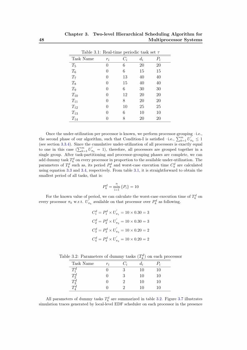
48Chapter 3. Two-level Hierarchical Scheduling Algorithm for
Multiprocessor Systems
Table 3.1: Real-time periodic task set τTask Name ri Ci di Pi
T5 0 6 20 20T6 0 6 15 15T7 0 13 40 40T8 0 15 40 40T9 0 6 30 30T10 0 12 20 20T11 0 8 20 20T12 0 10 25 25T13 0 6 10 10T14 0 8 20 20
Once the under-utilization per processor is known, we perform processor-grouping –i.e.,the second phase of our algorithm, such that Condition-I is satisfied –i.e.,
∑mk=1 U
′
πk≤ 1
(see section 3.3.4). Since the cumulative under-utilization of all processors is exactly equalto one in this case (
∑mk=1 U
′
πk= 1), therefore, all processors are grouped together in a
single group. After task-partitioning and processor-grouping phases are complete, we canadd dummy task T dk on every processor in proportion to the available under-utilization. Theparameters of T dk such as, its period P dk and worst-case execution time Cdk are calculatedusing equation 3.3 and 3.4, respectively. From table 3.1, it is straightforward to obtain thesmallest period of all tasks, that is:
P dk =n
mini=1{Pi} = 10
For the known value of period, we can calculate the worst-case execution time of T dk onevery processor πk w.r.t. U
′
πkavailable on that processor over P dk as following.
Cd1 = P d1 × U′
π1= 10× 0.30 = 3
Cd2 = P d2 × U′
π2= 10× 0.30 = 3
Cd3 = P d3 × U′
π3= 10× 0.20 = 2
Cd4 = P d4 × U′
π4= 10× 0.20 = 2
Table 3.2: Parameters of dummy tasks (T dk ) on each processorTask Name ri Ci di Pi
T d1 0 3 10 10T d2 0 3 10 10T d3 0 2 10 10T d4 0 2 10 10
All parameters of dummy tasks T dk are summarized in table 3.2. Figure 3.7 illustratessimulation traces generated by local-level EDF scheduler on each processor in the presence
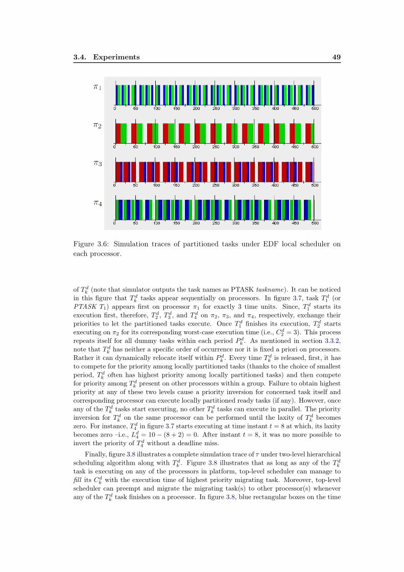
3.4. Experiments 49
Figure 3.6: Simulation traces of partitioned tasks under EDF local scheduler oneach processor.
of T dk (note that simulator outputs the task names as PTASK taskname). It can be noticedin this figure that T dk tasks appear sequentially on processors. In figure 3.7, task T d1 (orPTASK T1) appears first on processor π1 for exactly 3 time units. Since, T d1 starts itsexecution first, therefore, T d2 , T d3 , and T d4 on π2, π3, and π4, respectively, exchange theirpriorities to let the partitioned tasks execute. Once T d1 finishes its execution, T d2 startsexecuting on π2 for its corresponding worst-case execution time (i.e., Cd2 = 3). This processrepeats itself for all dummy tasks within each period P dk . As mentioned in section 3.3.2,note that T dk has neither a specific order of occurrence nor it is fixed a priori on processors.Rather it can dynamically relocate itself within P dk . Every time T dk is released, first, it hasto compete for the priority among locally partitioned tasks (thanks to the choice of smallestperiod, T dk often has highest priority among locally partitioned tasks) and then competefor priority among T dk present on other processors within a group. Failure to obtain highestpriority at any of these two levels cause a priority inversion for concerned task itself andcorresponding processor can execute locally partitioned ready tasks (if any). However, onceany of the T dk tasks start executing, no other T dk tasks can execute in parallel. The priorityinversion for T dk on the same processor can be performed until the laxity of T dk becomeszero. For instance, T d4 in figure 3.7 starts executing at time instant t = 8 at which, its laxitybecomes zero –i.e., Ld4 = 10 − (8 + 2) = 0. After instant t = 8, it was no more possible toinvert the priority of T d4 without a deadline miss.
Finally, figure 3.8 illustrates a complete simulation trace of τ under two-level hierarchicalscheduling algorithm along with T dk . Figure 3.8 illustrates that as long as any of the T dktask is executing on any of the processors in platform, top-level scheduler can manage tofill its Cdk with the execution time of highest priority migrating task. Moreover, top-levelscheduler can preempt and migrate the migrating task(s) to other processor(s) wheneverany of the T dk task finishes on a processor. In figure 3.8, blue rectangular boxes on the time
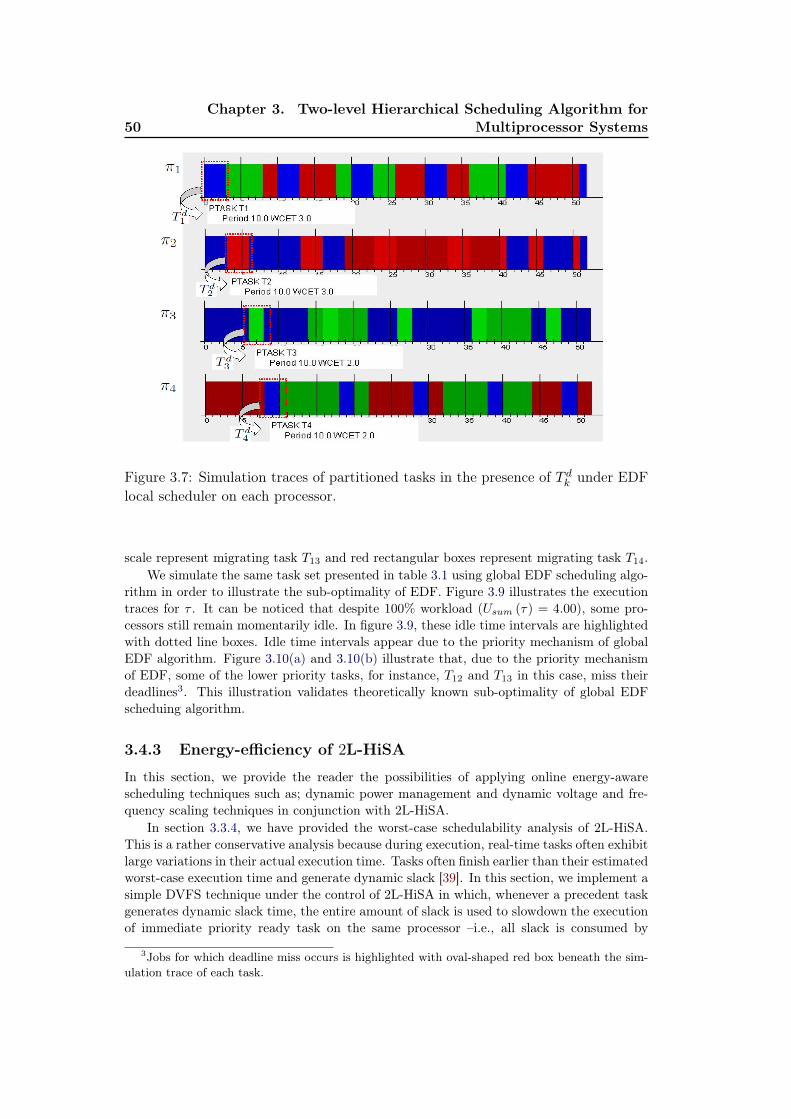
50Chapter 3. Two-level Hierarchical Scheduling Algorithm for
Multiprocessor Systems
Figure 3.7: Simulation traces of partitioned tasks in the presence of T dk under EDFlocal scheduler on each processor.
scale represent migrating task T13 and red rectangular boxes represent migrating task T14.We simulate the same task set presented in table 3.1 using global EDF scheduling algo-
rithm in order to illustrate the sub-optimality of EDF. Figure 3.9 illustrates the executiontraces for τ . It can be noticed that despite 100% workload (Usum (τ) = 4.00), some pro-cessors still remain momentarily idle. In figure 3.9, these idle time intervals are highlightedwith dotted line boxes. Idle time intervals appear due to the priority mechanism of globalEDF algorithm. Figure 3.10(a) and 3.10(b) illustrate that, due to the priority mechanismof EDF, some of the lower priority tasks, for instance, T12 and T13 in this case, miss theirdeadlines3. This illustration validates theoretically known sub-optimality of global EDFscheduing algorithm.
3.4.3 Energy-efficiency of 2L-HiSA
In this section, we provide the reader the possibilities of applying online energy-awarescheduling techniques such as; dynamic power management and dynamic voltage and fre-quency scaling techniques in conjunction with 2L-HiSA.
In section 3.3.4, we have provided the worst-case schedulability analysis of 2L-HiSA.This is a rather conservative analysis because during execution, real-time tasks often exhibitlarge variations in their actual execution time. Tasks often finish earlier than their estimatedworst-case execution time and generate dynamic slack [39]. In this section, we implement asimple DVFS technique under the control of 2L-HiSA in which, whenever a precedent taskgenerates dynamic slack time, the entire amount of slack is used to slowdown the executionof immediate priority ready task on the same processor –i.e., all slack is consumed by
3Jobs for which deadline miss occurs is highlighted with oval-shaped red box beneath the sim-ulation trace of each task.
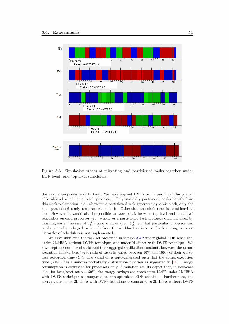
3.4. Experiments 51
Figure 3.8: Simulation traces of migrating and partitioned tasks together underEDF local- and top-level schedulers.
the next appropriate priority task. We have applied DVFS technique under the controlof local-level scheduler on each processor. Only statically partitioned tasks benefit fromthis slack reclamation –i.e., whenever a partitioned task generates dynamic slack, only thenext partitioned ready task can consume it. Otherwise, the slack time is considered aslost. However, it would also be possible to share slack between top-level and local-levelschedulers on each processor –i.e., whenever a partitioned task produces dynamic slack byfinishing early, the size of T dk ’s time window (i.e., Cdk) on that particular processor canbe dynamically enlarged to benefit from the workload variations. Slack sharing betweenhierarchy of schedulers is not implemented.
We have simulated the task set presented in section 3.4.2 under global EDF scheduler,under 2L-HiSA without DVFS technique, and under 2L-HiSA with DVFS technique. Wehave kept the number of tasks and their aggregate utilization constant, however, the actualexecution time or bcet/wcet ratio of tasks is varied between 50% and 100% of their worst-case execution time (Ci). The variation is auto-generated such that the actual executiontime (AET) has a uniform probability distribution function as suggested in [11]. Energyconsumption is estimated for processors only. Simulation results depict that, in best-case–i.e., for bcet/wcet ratio = 50%, the energy savings can reach upto 42.6% under 2L-HiSAwith DVFS technique as compared to non-optimized EDF schedule. Furthermore, theenergy gains under 2L-HiSA with DVFS technique as compared to 2L-HiSA without DVFS
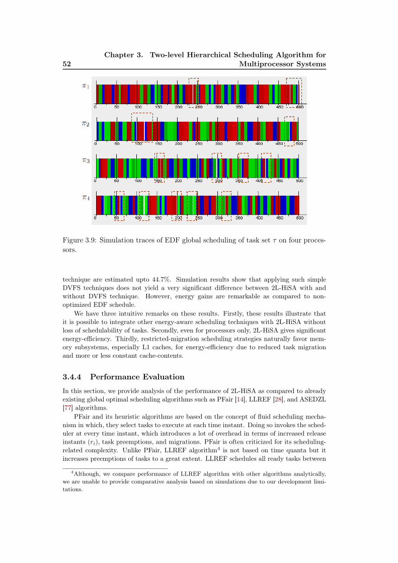
52Chapter 3. Two-level Hierarchical Scheduling Algorithm for
Multiprocessor Systems
Figure 3.9: Simulation traces of EDF global scheduling of task set τ on four proces-sors.
technique are estimated upto 44.7%. Simulation results show that applying such simpleDVFS techniques does not yield a very significant difference between 2L-HiSA with andwithout DVFS technique. However, energy gains are remarkable as compared to non-optimized EDF schedule.
We have three intuitive remarks on these results. Firstly, these results illustrate thatit is possible to integrate other energy-aware scheduling techniques with 2L-HiSA withoutloss of schedulability of tasks. Secondly, even for processors only, 2L-HiSA gives significantenergy-efficiency. Thirdly, restricted-migration scheduling strategies naturally favor mem-ory subsystems, especially L1 caches, for energy-efficiency due to reduced task migrationand more or less constant cache-contents.
3.4.4 Performance Evaluation
In this section, we provide analysis of the performance of 2L-HiSA as compared to alreadyexisting global optimal scheduling algorithms such as PFair [14], LLREF [28], and ASEDZL[77] algorithms.
PFair and its heuristic algorithms are based on the concept of fluid scheduling mecha-nism in which, they select tasks to execute at each time instant. Doing so invokes the sched-uler at every time instant, which introduces a lot of overhead in terms of increased releaseinstants (ri), task preemptions, and migrations. PFair is often criticized for its scheduling-related complexity. Unlike PFair, LLREF algorithm4 is not based on time quanta but itincreases preemptions of tasks to a great extent. LLREF schedules all ready tasks between
4Although, we compare performance of LLREF algorithm with other algorithms analytically,we are unable to provide comparative analysis based on simulations due to our development limi-tations.

3.4. Experiments 53
(a) Simulation traces for T5 − T9.
(b) Simulation traces for T10 − T14.
Figure 3.10: Simulation traces of individual tasks under global EDF scheduler
any two release instants. Since all tasks are active at all time instants, therefore, context-switching overhead and cache-related preemption delay is significantly large for LLREF.ASEDZL algorithm, contrary to PFair, is not based on time quanta. Execution require-ment and time periods of tasks can have any arbitrary value under ASEDZL algorithm.It improves on LLREF algorithm by scheduling minimum number of tasks between any

54Chapter 3. Two-level Hierarchical Scheduling Algorithm for
Multiprocessor Systems
two release instants. However, it still incurs higher number of scheduling events and pre-emptions than EDF scheduler. 2L-HiSA scheduling algorithm uses multiple instances ofsingle-processor optimal EDF algorithm to schedule tasks both at top-level and local-levelschedulers. Since, EDF invokes the scheduler only at job boundaries, therefore, the overheadin terms of release instants and number of preemptions is much less than the techniquesdiscussed earlier. Furthermore, 2L-HiSA has reduced overhead of L1 cache memories dueto the limited number of context-switches. Most of the tasks are partitioned under thisalgorithm, which limits the number of task migrations (only migrating or global sub-set oftasks migrate). Thus, the caches are mostly occupied by partitioned tasks, which helps inreducing the recovery time that a task may suffer from cache-miss and eventually improveperformance.
Figure 3.11: Number of task preemptions under 2L-HiSA, PFair (PD2), andASEDZL algorithms.
We compare the number of task preemptions and task migrations under 2L-HiSA, PD2
PFair algorithm [6], and ASEDZL [77] algorithms for the task set presented in table 3.1 overa simulation time equal to one hyper-period –i.e., 600 time units. Figure 3.11 illustratesthat the number of preemptions under PD2 PFair algorithm for various number of tasksis the highest. We have estimated an average difference of 15-fold between preemptionsunder PD2 PFair and ASEDZL and an average difference of 18-fold between PD2 PFairand 2L-HiSA. An average difference in the number of preemption between ASEDZL and2L-HiSA has been estimated up to 1.3-fold. Note that these results take into account thepreemptions of tasks under every local-level scheduler as well as top-level scheduler whileusing 2L-HiSA. Similarly, figure 3.12 illustrates the number of task migrations for variousnumber of tasks. Still, migration of tasks under PD2 PFair algorithm is relatively veryhigh. We have estimated an average difference of 4-fold between task migration under PD2
PFair and ASEDZL and an average difference of 10-fold between PD2 PFair and 2L-HiSA.An average difference in the number of task migration between ASEDZL and 2L-HiSA has
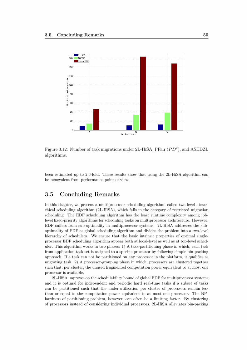
3.5. Concluding Remarks 55
Figure 3.12: Number of task migrations under 2L-HiSA, PFair (PD2), and ASEDZLalgorithms.
been estimated up to 2.6-fold. These results show that using the 2L-HiSA algorithm canbe benevolent from performance point of view.
3.5 Concluding Remarks
In this chapter, we present a multiprocessor scheduling algorithm, called two-level hierar-chical scheduling algorithm (2L-HiSA), which falls in the category of restricted migrationscheduling. The EDF scheduling algorithm has the least runtime complexity among job-level fixed-priority algorithms for scheduling tasks on multiprocessor architecture. However,EDF suffers from sub-optimality in multiprocessor systems. 2L-HiSA addresses the sub-optimality of EDF as global scheduling algorithm and divides the problem into a two-levelhierarchy of schedulers. We ensure that the basic intrinsic properties of optimal single-processor EDF scheduling algorithm appear both at local-level as well as at top-level sched-uler. This algorithm works in two phases: 1) A task-partitioning phase in which, each taskfrom application task set is assigned to a specific processor by following simple bin-packingapproach. If a task can not be partitioned on any processor in the platform, it qualifies asmigrating task. 2) A processor-grouping phase in which, processors are clustered togethersuch that, per cluster, the unused fragmented computation power equivalent to at most oneprocessor is available.
2L-HiSA improves on the schedulability bound of global EDF for multiprocessor systemsand it is optimal for independent and periodic hard real-time tasks if a subset of taskscan be partitioned such that the under-utilization per cluster of processors remain lessthan or equal to the computation power equivalent to at most one processor. The NP-hardness of partitioning problem, however, can often be a limiting factor. By clusteringof processors instead of considering individual processors, 2L-HiSA alleviates bin-packing

56Chapter 3. Two-level Hierarchical Scheduling Algorithm for
Multiprocessor Systems
limitations by effectively increasing bin sizes in comparison to item sizes. With a cluster ofprocessors, it is much easier to obtain the under-utilization per cluster less than or equalto the computation power equivalent to one processor. This chapter provides simulationresults to support our proposition. We have illustrated that power- and energy-efficientstrategies like DVFS and/or DPM can be used in conjunction with 2L-HiSA to improveenergy savings. Furthermore, we have illustrated that the task preemption- and migration-related overhead is significantly less while using 2L-HiSA as scheduling algorithm.
Chapter 4
Assertive Dynamic PowerManagement Technique
Contents4.1 Dynamic Power Management . . . . . . . . . . . . . . . . . . 57
4.2 Related Work . . . . . . . . . . . . . . . . . . . . . . . . . . . . 58
4.3 Assertive Dynamic Power Management Technique . . . . . 61
4.3.1 Laxity Bottom Test (LBT) . . . . . . . . . . . . . . . . . . . 62
4.3.2 Working Principle . . . . . . . . . . . . . . . . . . . . . . . . 64
4.3.3 Choice of Power-efficient State . . . . . . . . . . . . . . . . . 68
4.4 Static Optimizations using AsDPM . . . . . . . . . . . . . . 69
4.5 Experiments . . . . . . . . . . . . . . . . . . . . . . . . . . . . 69
4.5.1 Target Application . . . . . . . . . . . . . . . . . . . . . . . . 69
4.5.2 Simulation Results . . . . . . . . . . . . . . . . . . . . . . . . 73
4.5.3 Comparative Analysis of the AsDPM Technique . . . . . . . 78
4.6 Future Perspectives of the AsDPM Technique . . . . . . . . 79
4.6.1 Memory Subsystem . . . . . . . . . . . . . . . . . . . . . . . 80
4.6.2 Thermal Load Balancing . . . . . . . . . . . . . . . . . . . . 82
4.7 Concluding Remarks . . . . . . . . . . . . . . . . . . . . . . . 84
4.1 Dynamic Power Management
Dynamic Power Management(DPM) techniques achieve energy conservation in embeddedcomputing systems by actively changing the power consumption profile of the system byselectively putting its components into power-efficient states sufficient to meeting function-ality requirements [57]. These techniques, when applied, exploit the inherently present idletime intervals (if any) in the real-time schedule of target application over a specific targetarchitecture at runtime. The idle time intervals can exist due to the variations in actualworkload at runtime or they can be statically present due to under-utilization of targetplatform. Optimality of DPM techniques depends on the workload statistics. Based onthese statistics, the effectiveness of different DPM techniques vary.
In this chapter, we present a DPM technique for multiprocessor real-time systems,called the Assertive Dynamic Power Management (AsDPM) technique. This techniqueis intended for multiprocessor real-time platforms of type SMP and it works under the
58 Chapter 4. Assertive Dynamic Power Management Technique
control of global EDF and LLF scheduling algorithms1. Our proposed technique is calledassertive DPM technique because of its aggressiveness in extracting the idle time intervals (ifpresent) from the application’s runtime schedule, which is not the case in conventional DPMtechniques. The working principle presented in section 4.3 further elaborates this aspect.Apart from being a DPM technique for processors, AsDPM can be useful in optimizingenergy consumption at memory subsystem level as well. Moreover, the AsDPM techniquecan be used, based on the workload characteristics, for statically (offline) optimizing thenumber of processors and their corresponding operating frequency and voltage level in amultiprocessor system. As a future perspective, we discuss how heat dissipation can beregulated while using this technique. Rest of this chapter is arranged as follows. In section4.2, we review state-of-the-art on DPM techniques. AsDPM is presented in detail in section4.3. Use of AsDPM for static optimizations in discussed in section 4.4. Experimentalevaluation is presented in section 4.5. Section 4.6 provides a brief discussion on ongoingand future perspectives of the AsDPM technique.
4.2 Related Work
In two different surveys of DPM techniques presented in [16] and [102], authors classify DPMtechniques into two main categories: predictive schemes and stochastic schemes. Predictiveschemes attempt to predict the timing of future input events to the system and scheduleshutdown (usually to a single power-efficient state) based on these predictions. Usually, notmuch is known regarding future input events in an online schedule and DPM decisions haveto be taken based on these so called uncertain predictions. The rationale in all predictiveschemes is to exploit the correlation between past history of the workload and its nearfuture in order to make reliable predictions about future events [53, 102]. The most commonpredictive DPM policy is the fixed timeout DPM policy, which uses the elapsed idle time asobserved event to predict the total duration of the current idle period. Such policies haveobvious advantage of being general and their safety can be improved simply by increasingthe timeout values. The obvious disadvantage of these techniques is that they trade-offefficiency for safety: large timeouts cause a large number of under-predictions, that representmissed opportunity of saving power, and a sizable amount of power is wasted waiting for thetimeout to expire. The predictive shutdown policies improve upon timeout-based schemesby taking decisions as soon as a new idle period starts, based on the observation of past idleand busy periods. One of the early research work on such techniques was presented in [107]in which, authors have proposed a predictive DPM technique for event-driven applications.The basic idea in [107] is to predict the length of idle periods and shutdown the systemwhen the predicted idle period is long enough to amortize the cost (in latency and power)of shutting down and later reactivating the system. A shortcoming of predictive shutdownapproach is that it is based on offline analysis of usage traces, hence it is not suitable for non-stationary workload whose statistical properties are not known a priori. This shortcomingis addressed by Hwang and Wu in [53]. They proposed online adaptive methods thatpredict the duration of an idle period with an exponentially weighted average of previousidle periods. Predictive DPM techniques improve on performance penalty as well, thatis always paid on wakeup, by performing predictive wakeup when the predicted idle timeexpires, even if no new task service requests have arrived. This choice may increase power
1Although we have implemented the AsDPM technique with both the EDF and the LLF schedul-ing algorithms, rest of this chapter will consider only EDF being the controlling scheduling algo-rithm.
4.2. Related Work 59
dissipation if idle time has been under-predicted, but decreases the delay for servicing thefirst incoming request after an idle period.
In some relatively recent work, researches have addressed the problem of inaccuratepredictions in DPM strategies in the real-time context. In real-time systems, predictingthe next time instant when a device will be needed is crucial not only because it is thekey for effective energy management, but also because inaccurate predictions may hurt thefeasibility of the system, in view of the non-trivial activation/de-activation delays. Hence,the real- time DPM has a number of unique characteristics. Authors in [112, 109] have pro-posed heuristic-based DPM schemes that can be used with both EDF and RMS schedulingpolices. However, the schemes consider only non-preemptive real-time task execution. Inanother work presented in [110], the same group of authors present an offline scheme, calledMaximum Device Overlap (MDO), for preemptive task scheduling. The MDO algorithmuses a real-time scheduling algorithm, e.g., EDF, to generate a feasible real-time job sched-ule and then iteratively swaps job segments to reduce energy consumption in device powerstate transitions. After the heuristic-based job schedule is generated, the device scheduleis extracted. That is, device power state transition actions and times are recorded priorto runtime and used at runtime. However, a problem with MDO is that the schedule isgenerated with jobs’ WCET. Even without resource blocking, the actual job executionscan be very different from the pre-generated job schedule. A fixed device schedule cannoteffectively adapt to changes in the operating environment, such as if dynamic task join orjobs complete early. Moreover, MDO involves very high time complexity (proportional tothe square of the hyper-period) and it cannot be successfully adapted to dynamic/onlinesettings where job release and execution times can vary considerably. Adaptive predictiveDPM techniques have also been proposed to deal with non-stationary workloads [102].
In another recent research work presented in [36], authors have proposed their solutionto the online real- time DPM problem, which is based on the observation that creatinglong device sleep intervals is the key for effective power management. Authors proposeto explicitly and periodically enforce such intervals for each system’s device at run time.These intervals, called the device forbidden regions (DFRs), enable the system to put thesedevices to sleep states. Authors propose to determine parameters, such as duration andseparation time of DFRs, through static analysis. Authors also ensure that none of thestatically determined DFRs should have its duration shorter than the device’s break-eventimes. This approach, however, can only exploit the inherently present idle time intervals inthe offline schedule to determine DFRs. Moreover, during a forbidden region, none of thetasks using the related device can be dispatched; hence, the duration and period of DFRsmust be carefully selected to preserve temporal correctness. This limits the possibility offully exploiting the offline slack time. The proposed approach in [36] is unable to exploitthe online slack time (online slack time can be generated due to the early completion oftasks) that can be used for further enlargement of device sleep intervals at runtime. Thesame authors have extended their DFR-based DPM solution to a unified framework in [35].The proposed framework, called DFR-EDF, assumes a general system- level energy modeland includes both static and dynamic (online) components. The static part is based onthe extension of their work in [36] for preemptive EDF scheduling. The online componentintegrates the predictive DPM techniques and offers a generalized slack reclaiming mech-anism that can be used by DVFS and DPM simultaneously. This framework is intendedfor system-wide energy-efficiency. In this work, authors claim to develop a unified energymanagement framework for deadline-driven periodic real-time applications by exploitingthe interplay between DVFS and DPM with both static and dynamic (runtime) solutioncomponents. This interplay of DPM and DVFS techniques, however, is not completely

60 Chapter 4. Assertive Dynamic Power Management Technique
online and adaptive. DPM is mainly used for static optimizations using device forbiddenregions.
Stochastic DPM techniques, rather than eliminating uncertainty by prediction, formu-late policy optimization as an optimization problem under uncertainty [18, 57, 84]. Morespecifically, power management optimization has been studied within the framework of con-trolled Markov processes. In this case, it is assumed that the system and the workload canbe modeled as Markov chains [16, 55]. Under this assumption, it is possible to: modelthe uncertainty in system power consumption and response (transition) times; model com-plex systems with many power states, buffers, queues, etc.; compute power managementpolicies that are globally optimum; explore trade-offs between power and performance ina controlled fashion. Stochastic optimum control is a well-researched category of DPMtechniques [29, 90, 100]. These techniques have several advantages over predictive tech-niques. First, it captures the global view of the system, thus allowing the designer to searchfor a global optimum that possibly exploits multiple inactive states of multiple interactingresources. Second, it enables the exact solution (in polynomial time) of the performance-constrained power optimization problem. Third, it exploits the strength and optimality ofrandomized policies [29, 83]. However, stochastic optimization techniques assume completea priori knowledge of the system and its workload statistics which can be a limiting factorin some cases. Even though it is generally possible to construct a model for the systemonce for all, the workload is generally much harder to characterize in advance. Furthermore,workloads are often non-stationary.
DPM techniques can be applied at several different levels in a system such as atprocessor-level, at peripheries, or a combination of both. Previously, significant amountof research has focused on applying (both predictive and stochastic) DPM techniques oneither processors only [18, 29, 55, 57, 100] or on peripheral devices only [26, 113]. However,system-wide energy conservation has received little attention. Some recent research workhas focused on applying DPM techniques together on processors as well as other systemcomponents such as peripheral or I/O devices, memory subsystems, flash drives, andwireless network interfaces in order to achieve system-wide energy savings. Authors in [27]suggest that these devices are pervasive in modern embedded systems which consume con-siderable amount of energy. Authors in [27] propose an online system-wide energy-efficientscheduling algorithm called SYS-EDF, which integrates dynamic power management forI/O devices and dynamic voltage scaling for the processor. SYS-EDF algorithm supportsperiodic task sets with non-preemptive shared resources. This algorithm takes advantageof slowed-down execution of tasks on processors by applying DVS on processors andconsequently, elongated idle periods on unused I/O devices.
The AsDPM technique considers mainly the processors for power and energy consump-tion optimization. It is not based on predictive mechanisms that predict either the arrivaltime or the length of an already arrived idle interval. Rather, it works on the principle ofadmission control for ready tasks by delaying the execution of ready tasks as much as pos-sible, thereby controlling the maximum number of active/running processors in the systemat any time instant. Tasks are delayed based on their remaining runtime laxity in a deter-ministic way. Section 4.3 further elaborates this concept. Although AsDPM is also basedon on the observation that creating long device sleep intervals is the key for effective powermanagement, unlike presented in [36], AsDPM is not based on device forbidden regions.Moreover, it can be used to exploit statically present idle time intervals as well as dynamicslack time generated by the early completion of tasks. Unlike [36] and [35], AsDPM doesnot need to be coupled with other DVFS or predictive DPM techniques in order to exploit
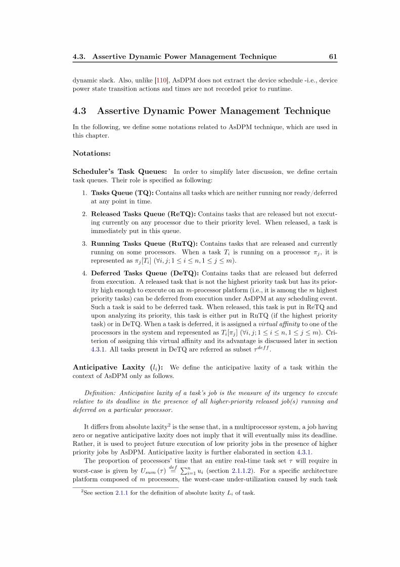
4.3. Assertive Dynamic Power Management Technique 61
dynamic slack. Also, unlike [110], AsDPM does not extract the device schedule -i.e., devicepower state transition actions and times are not recorded prior to runtime.
4.3 Assertive Dynamic Power Management Technique
In the following, we define some notations related to AsDPM technique, which are used inthis chapter.
Notations:
Scheduler’s Task Queues: In order to simplify later discussion, we define certaintask queues. Their role is specified as following:
1. Tasks Queue (TQ): Contains all tasks which are neither running nor ready/deferredat any point in time.
2. Released Tasks Queue (ReTQ): Contains tasks that are released but not execut-ing currently on any processor due to their priority level. When released, a task isimmediately put in this queue.
3. Running Tasks Queue (RuTQ): Contains tasks that are released and currentlyrunning on some processors. When a task Ti is running on a processor πj , it isrepresented as πj [Ti] (∀i, j; 1 ≤ i ≤ n, 1 ≤ j ≤ m).
4. Deferred Tasks Queue (DeTQ): Contains tasks that are released but deferredfrom execution. A released task that is not the highest priority task but has its prior-ity high enough to execute on an m-processor platform (i.e., it is among the m highestpriority tasks) can be deferred from execution under AsDPM at any scheduling event.Such a task is said to be deferred task. When released, this task is put in ReTQ andupon analyzing its priority, this task is either put in RuTQ (if the highest prioritytask) or in DeTQ. When a task is deferred, it is assigned a virtual affinity to one of theprocessors in the system and represented as Ti[πj ] (∀i, j; 1 ≤ i ≤ n, 1 ≤ j ≤ m). Cri-terion of assigning this virtual affinity and its advantage is discussed later in section4.3.1. All tasks present in DeTQ are referred as subset τdeff .
Anticipative Laxity (li): We define the anticipative laxity of a task within thecontext of AsDPM only as follows.
Definition: Anticipative laxity of a task’s job is the measure of its urgency to executerelative to its deadline in the presence of all higher-priority released job(s) running anddeferred on a particular processor.
It differs from absolute laxity2 is the sense that, in a multiprocessor system, a job havingzero or negative anticipative laxity does not imply that it will eventually miss its deadline.Rather, it is used to project future execution of low priority jobs in the presence of higherpriority jobs by AsDPM. Anticipative laxity is further elaborated in section 4.3.1.
The proportion of processors’ time that an entire real-time task set τ will require inworst-case is given by Usum (τ)
def=∑ni=1 ui (section 2.1.1.2). For a specific architecture
platform composed of m processors, the worst-case under-utilization caused by such task
2See section 2.1.1 for the definition of absolute laxity Li of task.

62 Chapter 4. Assertive Dynamic Power Management Technique
set is m− Usum(τ). This under-utilization appears at runtime in the form of random andvariable length idle time intervals on different processors for non-stationary workload. Aconventional DPM technique, whether predictive or stochastic, can exploit these idle inter-vals only once they occur on a processor –i.e., once an idle interval is detected. Upon de-tecting idle time intervals, these techniques decide whether to transition target processor(s)to power-efficient state. AsDPM, on the other hand, differs from the existing techniques inthe way it exploits idle time intervals. It aggressively extracts all idle time intervals fromsome processors (let us say k processors) and clusters them on some other processors (letus say m-k processors) to elongate the duration of idle time on m − k processors. Tran-sitioning these m − k processors to suitable power-efficient state then becomes a matterof comparing idle interval’s length against the break-even time (BET) of target processor.It is worth mentioning here that AsDPM is an admission control technique for real-timetasks that makes a feasible task set energy-efficient by deciding when exactly a ready taskshall execute. Without this admission control, all ready tasks are executed as soon asthere are enough computing resources (processors) available in the system, leading to poorpossibilities of putting some system components in power-efficient states. AsDPM worksonly in conjunction with multiprocessor global scheduling algorithms. Moreover, it doesnot intervene in the priority-related decision making of the scheduling algorithm. That is,the priority order of all tasks, whether deferred or executing, is preserved while using As-DPM in conjunction with global scheduling algorithms. However, a released lower priorityjob may be deferred/delayed from execution unless its urgency level becomes critical. Inorder to control the admission of tasks into RuTQ, AsDPM performs a test, called LaxityBottom Test (LBT), on all released jobs of tasks (except the highest priority job) at everyscheduling event.
4.3.1 Laxity Bottom Test (LBT)
Laxity bottom test is performed at every scheduling event for all tasks (except the highestpriority job) present in ReTQ. It is based on the anticipative laxity li of tasks. Everytime LBT is performed, at first, it is assumed that at most one processor is running in thesystem3 (i.e., present in active state) at current scheduling event that invoked the scheduler.This assumption allows to assign (and/or defer) maximum tasks on one processor as longas possible. The highest priority ready task from ReTQ is assigned to processor directlyfor execution and for all remaining ready jobs in ReTQ, LBT is performed. LBT worksas follows. If the anticipative laxity of a ready job results in a negative value (< 0) thenthe test is said to be failed for that job and the job would miss its deadline if no furthercomputing resources are provided (i.e., processor must be activated). On the other hand, ifLBT passes for a task –i.e., the anticipative laxity results in a positive value (≥ 0) then thejob in question can still meet its deadline in future, if it would be deferred from executionat current scheduling event (until the next event). LBT ensures deadlines for all releasedjobs between successive scheduling events. In the following, we describe how anticipativelaxity is calculated.
Recall the definition of anticipative laxity from section 4.3, which states that all higherpriority released and deferred tasks should be considered while calculating the value ofanticipative laxity li of a particular low priority task Ti on a target processor πj . In amultiprocessor system, where tasks may execute in parallel, multiple higher priority tasks
3There can be more than one processors running in the system. This is just an assumption tostart the LBT test. Once the LBT is complete for all tasks, resulting number of required runningprocessors can be the same as previously available or it may be different.

4.3. Assertive Dynamic Power Management Technique 63
(than Ti) might be simultaneously running on different processors and some higher prioritytasks might be already present in τdeff . Moreover, some or all higher priority tasks mighthave already completed a portion of their execution requirement (C), therefore, only theremaining execution requirement (Crem) of higher priority tasks shall be considered forcalculating li. Since all higher priority tasks are not supposed to run on πj sequentially(rather, there will be at most (m− 1) higher priority tasks running in parallel), therefore,considering the Crem of all higher priority tasks would result in a very pessimistic value ofli on πj . To avoid this pessimism in calculation, anticipative laxity li of task Ti is calculatedon processor πj in the presence of only those higher priority tasks which are either currentlyrunning on πj or are deferred earlier with an associativity with πj processor –i.e., Tk[πj ]
(∀k; i < k). Here, Tk refers to any task having higher priority than Ti and currentlyrunning or deferred on processor πj . Equation 4.1 illustrates how li for task Ti is calculatedon processor πj in the presence of higher priority tasks.
li = di −
t+ Cremj + Cremi +∑
Tk[πj ]∈τdeffCremk
(4.1)
In equation 4.1, t refers to the time instant at which the scheduling event has occurred,Cremi refers to the remaining execution time of task Ti for which li is calculated, Cremj refersto the remaining execution time of task which is currently running on processor πj , and Cremk
refers to the remaining execution time of all higher priority deferred tasks present in τdeff
having an affinity with processor πj . When a task is deferred –i.e., its LBT is passed on aprocessor, the task is assigned a affinity to that processor. This affinity is valid between twosuccessive scheduling events only as the LBT is performed again at next scheduling event.The purpose of assigning this affinity is to make the calculation of anticipative laxity non-pessimistic by avoiding the reconsideration of those higher priority tasks that are alreadybeing deferred to some other processors. Following example elaborates the working of LBTfurther.
Example–1: Let us consider a task set composed of three periodic, independent, andsynchronous tasks such that τ={T1, T2, T3}. The quadruplet (ri,Ci,di,Pi) values for T1,T2, and T3 are {0, 6, 12, 12}, {0, 8, 14, 14}, and {0, 5, 20, 20}, respectively. Task set τ isscheduled under preemtive EDF scheduling policy –i.e., smaller the deadline, greater thepriority. In figure 4.1, time instant tc marks a scheduling event at which all three taskjobs are released. According to the priority order, task T1 has the highest priority andit is directly assigned to processor πj for execution. At the same time instant tc = 0,LBT is performed on other two lower priority tasks. Using equation 4.1, the anticipativelaxity of task T2 –i.e., l2, in the presence of higher priority task T1 is non-negative –i.e., l2=14−(0 + 6 + 8 + 0)=0. This result shows that, at time instant tc = 0, task T2 can still meetits deadline if it will be executed after the worst-case completion of T1. Thus, T2 can bedeferred at this stage on processor πj –i.e., T2[πj ] at time tc = 0. Similarly, the anticipativelaxity of task T3 –i.e., l3, is calculated in the presence of higher priority tasks T1 and T2 suchthat, l3= 20− (0 + 5 + 8 + 6)>0. Like T2, T3 can also meet its deadline after the worst-casecompletion of T1 and T2 and therefore, can be deferred until next scheduling event occurs.Note that tasks T2 and T3 are shown dotted because this is only an anticipation of thefuture schedule of tasks at current scheduling event that may change upon the arrival ofnext event.
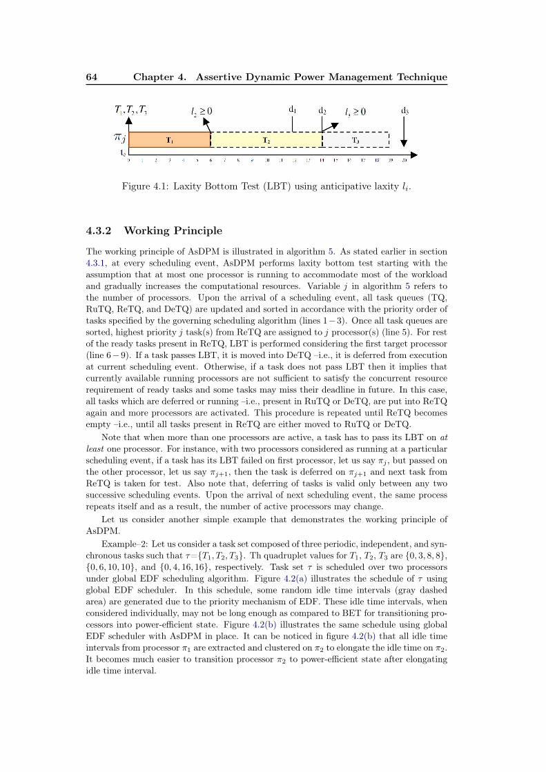
64 Chapter 4. Assertive Dynamic Power Management Technique
Figure 4.1: Laxity Bottom Test (LBT) using anticipative laxity li.
4.3.2 Working Principle
The working principle of AsDPM is illustrated in algorithm 5. As stated earlier in section4.3.1, at every scheduling event, AsDPM performs laxity bottom test starting with theassumption that at most one processor is running to accommodate most of the workloadand gradually increases the computational resources. Variable j in algorithm 5 refers tothe number of processors. Upon the arrival of a scheduling event, all task queues (TQ,RuTQ, ReTQ, and DeTQ) are updated and sorted in accordance with the priority order oftasks specified by the governing scheduling algorithm (lines 1−3). Once all task queues aresorted, highest priority j task(s) from ReTQ are assigned to j processor(s) (line 5). For restof the ready tasks present in ReTQ, LBT is performed considering the first target processor(line 6− 9). If a task passes LBT, it is moved into DeTQ –i.e., it is deferred from executionat current scheduling event. Otherwise, if a task does not pass LBT then it implies thatcurrently available running processors are not sufficient to satisfy the concurrent resourcerequirement of ready tasks and some tasks may miss their deadline in future. In this case,all tasks which are deferred or running –i.e., present in RuTQ or DeTQ, are put into ReTQagain and more processors are activated. This procedure is repeated until ReTQ becomesempty –i.e., until all tasks present in ReTQ are either moved to RuTQ or DeTQ.
Note that when more than one processors are active, a task has to pass its LBT on atleast one processor. For instance, with two processors considered as running at a particularscheduling event, if a task has its LBT failed on first processor, let us say πj , but passed onthe other processor, let us say πj+1, then the task is deferred on πj+1 and next task fromReTQ is taken for test. Also note that, deferring of tasks is valid only between any twosuccessive scheduling events. Upon the arrival of next scheduling event, the same processrepeats itself and as a result, the number of active processors may change.
Let us consider another simple example that demonstrates the working principle ofAsDPM.
Example–2: Let us consider a task set composed of three periodic, independent, and syn-chronous tasks such that τ={T1, T2, T3}. Th quadruplet values for T1, T2, T3 are {0, 3, 8, 8},{0, 6, 10, 10}, and {0, 4, 16, 16}, respectively. Task set τ is scheduled over two processorsunder global EDF scheduling algorithm. Figure 4.2(a) illustrates the schedule of τ usingglobal EDF scheduler. In this schedule, some random idle time intervals (gray dashedarea) are generated due to the priority mechanism of EDF. These idle time intervals, whenconsidered individually, may not be long enough as compared to BET for transitioning pro-cessors into power-efficient state. Figure 4.2(b) illustrates the same schedule using globalEDF scheduler with AsDPM in place. It can be noticed in figure 4.2(b) that all idle timeintervals from processor π1 are extracted and clustered on π2 to elongate the idle time on π2.It becomes much easier to transition processor π2 to power-efficient state after elongatingidle time interval.
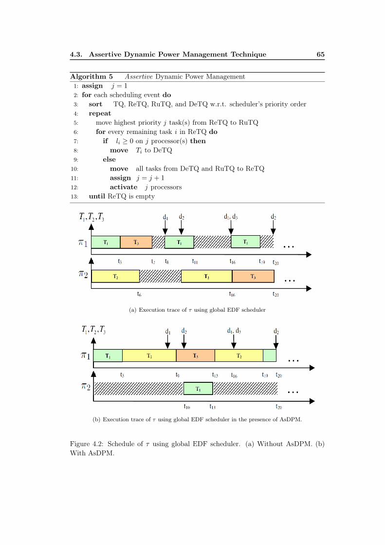
4.3. Assertive Dynamic Power Management Technique 65
Algorithm 5 Assertive Dynamic Power Management1: assign j = 1
2: for each scheduling event do3: sort TQ, ReTQ, RuTQ, and DeTQ w.r.t. scheduler’s priority order4: repeat5: move highest priority j task(s) from ReTQ to RuTQ6: for every remaining task i in ReTQ do7: if li ≥ 0 on j processor(s) then8: move Ti to DeTQ9: else
10: move all tasks from DeTQ and RuTQ to ReTQ11: assign j = j + 1
12: activate j processors13: until ReTQ is empty
(a) Execution trace of τ using global EDF scheduler
(b) Execution trace of τ using global EDF scheduler in the presence of AsDPM.
Figure 4.2: Schedule of τ using global EDF scheduler. (a) Without AsDPM. (b)With AsDPM.
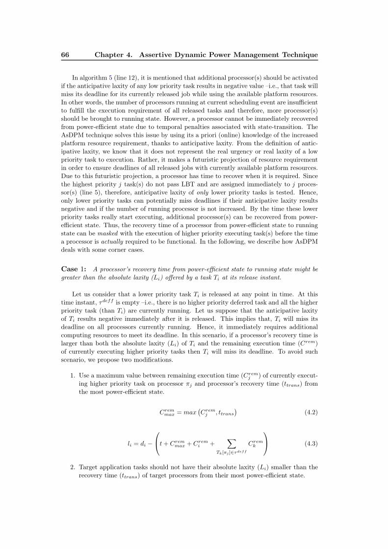
66 Chapter 4. Assertive Dynamic Power Management Technique
In algorithm 5 (line 12), it is mentioned that additional processor(s) should be activatedif the anticipative laxity of any low priority task results in negative value –i.e., that task willmiss its deadline for its currently released job while using the available platform resources.In other words, the number of processors running at current scheduling event are insufficientto fulfill the execution requirement of all released tasks and therefore, more processor(s)should be brought to running state. However, a processor cannot be immediately recoveredfrom power-efficient state due to temporal penalties associated with state-transition. TheAsDPM technique solves this issue by using its a priori (online) knowledge of the increasedplatform resource requirement, thanks to anticipative laxity. From the definition of antic-ipative laxity, we know that it does not represent the real urgency or real laxity of a lowpriority task to execution. Rather, it makes a futuristic projection of resource requirementin order to ensure deadlines of all released jobs with currently available platform resources.Due to this futuristic projection, a processor has time to recover when it is required. Sincethe highest priority j task(s) do not pass LBT and are assigned immediately to j proces-sor(s) (line 5), therefore, anticipative laxity of only lower priority tasks is tested. Hence,only lower priority tasks can potentially miss deadlines if their anticipative laxity resultsnegative and if the number of running processor is not increased. By the time these lowerpriority tasks really start executing, additional processor(s) can be recovered from power-efficient state. Thus, the recovery time of a processor from power-efficient state to runningstate can be masked with the execution of higher priority executing task(s) before the timea processor is actually required to be functional. In the following, we describe how AsDPMdeals with some corner cases.
Case 1: A processor’s recovery time from power-efficient state to running state might begreater than the absolute laxity (Li) offered by a task Ti at its release instant.
Let us consider that a lower priority task Ti is released at any point in time. At thistime instant, τdeff is empty –i.e., there is no higher priority deferred task and all the higherpriority task (than Ti) are currently running. Let us suppose that the anticipative laxityof Ti results negative immediately after it is released. This implies that, Ti will miss itsdeadline on all processors currently running. Hence, it immediately requires additionalcomputing resources to meet its deadline. In this scenario, if a processor’s recovery time islarger than both the absolute laxity (Li) of Ti and the remaining execution time (Crem)of currently executing higher priority tasks then Ti will miss its deadline. To avoid suchscenario, we propose two modifications.
1. Use a maximum value between remaining execution time (Cremj ) of currently execut-ing higher priority task on processor πj and processor’s recovery time (ttrans) fromthe most power-efficient state.
Cremmax = max(Cremj , ttrans
)(4.2)
li = di −
t+ Cremmax + Cremi +∑
Tk[πj ]∈τdeffCremk
(4.3)
2. Target application tasks should not have their absolute laxity (Li) smaller than therecovery time (ttrans) of target processors from their most power-efficient state.
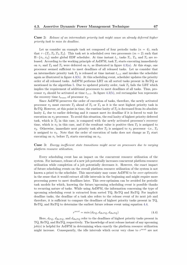
4.3. Assertive Dynamic Power Management Technique 67
Case 2: Release of an intermediate priority task might cause an already deferred higherpriority task to miss its deadline.
Let us consider an example task set composed of four periodic tasks (n = 4), suchthat τ={T1, T2, T3, T4}. This task set is scheduled over two processors (m = 2) such thatΠ={π1, π2} under global EDF scheduler. At time instant tc, tasks T1, T2, and T4 are re-leased. According to the working principle of AsDPM, task T1 starts executing immediatelyon π1 and T2 and T4 were deferred on π1 as illustrated in figure 4.3(a). At this stage, oneprocessor seemed sufficient to meet deadlines of all released tasks. Let us consider thatan intermediate priority task T3 is released at time instant tc+1 and invokes the scheduleragain as illustrated in figure 4.3(b). At this scheduling event, scheduler updates the priorityorder of all released tasks. AsDPM performs LBT on all sorted tasks present in ReTQ asmentioned in the algorithm 5. Due to updated priority order, task T4 fails the LBT whichimplies the requirement of additional processors to meet deadlines of all tasks. Thus, pro-cessor π2 should be activated at time tc+1. In figure 4.3(b), red rectangular box representsthe recovery time ttrans of processor π2.
Since AsDPM preserves the order of execution of tasks, therefore, the newly activatedprocessor π2 must execute T2 ahead of T3 or T4 as it is the next highest priority task inReTQ. However, at this point in time, the runtime laxity of T2 is decreased from its absolutelaxity Li due to earlier deferring and it cannot meet its deadline if it is forced to wait forexecution on π2 processor. To avoid this situation, the real laxity of highest priority deferredtask, which is T2 in this case, is compared with the newly activated processor’s recoverytime, which is π2 in this case, and if the resultant value is positive then T2 is assigned toπ2. Otherwise, immediate next priority task after T2 is assigned to π2 processor –i.e., T3is assigned to π2. Note that the order of execution of tasks does not change as T2 startexecuting on π1 before T3 starts executing on π2.
Case 3: Energy inefficient state transitions might occur on processors due to varyingplatform resource utilization.
Every scheduling event has an impact on the concurrent resource utilization of thesystem. For instance, release of a new job potentially increases concurrent platform resourceutilization while completion of a job potentially decreases it. However, the exact impactof future scheduling events on the overall platform resource utilization of the system is notknown a priori to the scheduler. This uncertainty may cause AsDPM to be over-optimisticin the sense that it would extract all idle intervals in the beginning and might require moreprocessing power to meet deadlines later. This over-optimism can be avoided for periodictask models for which, knowing the future/upcoming scheduling event is possible thanksto recurring nature of tasks. While using AsDPM, the information concerning the type ofupcoming scheduling event is extracted from sorted TQ, ReTQ and RuTQ. For implicitdeadline tasks, the deadline of a task also refers to the release event of its next job andtherefore, it is sufficient to compare the deadlines of highest priority tasks present in TQ,ReTQ, and RuTQ to determine the earliest future release event using equation 4.4.
rnext = min (dTQ, dReTQ, dRuTQ) (4.4)
Here, dTQ, dReTQ, and dRuTQ refer to the deadlines of highest priority tasks present inTQ, ReTQ, and RuTQ, respectively. The knowledge of next release instant of any upcomingjob(s) is helpful for AsDPM in determining when exactly the platform resource utilizationmight increase. Consequently, the idle intervals which occur very close to rnext are not
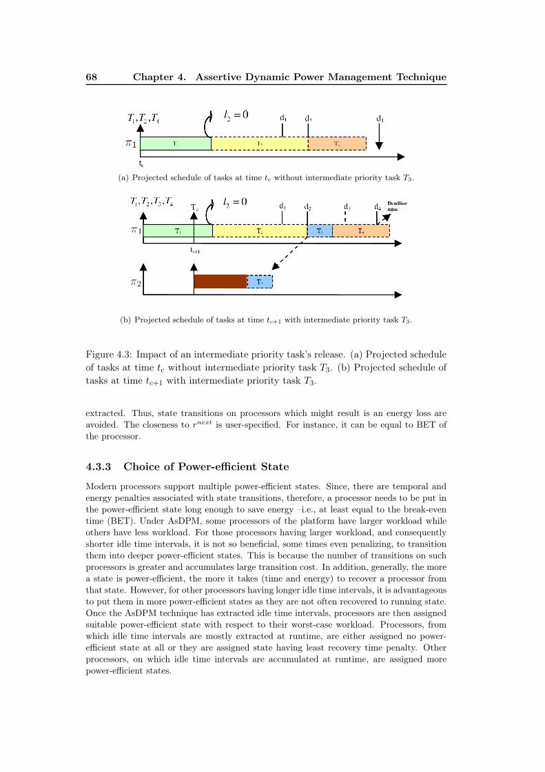
68 Chapter 4. Assertive Dynamic Power Management Technique
(a) Projected schedule of tasks at time tc without intermediate priority task T3.
(b) Projected schedule of tasks at time tc+1 with intermediate priority task T3.
Figure 4.3: Impact of an intermediate priority task’s release. (a) Projected scheduleof tasks at time tc without intermediate priority task T3. (b) Projected schedule oftasks at time tc+1 with intermediate priority task T3.
extracted. Thus, state transitions on processors which might result is an energy loss areavoided. The closeness to rnext is user-specified. For instance, it can be equal to BET ofthe processor.
4.3.3 Choice of Power-efficient State
Modern processors support multiple power-efficient states. Since, there are temporal andenergy penalties associated with state transitions, therefore, a processor needs to be put inthe power-efficient state long enough to save energy –i.e., at least equal to the break-eventime (BET). Under AsDPM, some processors of the platform have larger workload whileothers have less workload. For those processors having larger workload, and consequentlyshorter idle time intervals, it is not so beneficial, some times even penalizing, to transitionthem into deeper power-efficient states. This is because the number of transitions on suchprocessors is greater and accumulates large transition cost. In addition, generally, the morea state is power-efficient, the more it takes (time and energy) to recover a processor fromthat state. However, for other processors having longer idle time intervals, it is advantageousto put them in more power-efficient states as they are not often recovered to running state.Once the AsDPM technique has extracted idle time intervals, processors are then assignedsuitable power-efficient state with respect to their worst-case workload. Processors, fromwhich idle time intervals are mostly extracted at runtime, are either assigned no power-efficient state at all or they are assigned state having least recovery time penalty. Otherprocessors, on which idle time intervals are accumulated at runtime, are assigned morepower-efficient states.

4.4. Static Optimizations using AsDPM 69
4.4 Static Optimizations using AsDPM
In section 4.3, it has been mentioned that AsDPM itself is an online admission controltechnique which decides when exactly a ready task shall execute. Without this admissioncontrol, all ready tasks are executed as soon as there are enough computing resources (pro-cessors) available in the system. This feature of AsDPM not only helps optimizing theuse of platform resources in an online fashion, but also can be used for static/offline opti-mizations of platform resources. By optimized platform resources, we mean the minimumnumber of required processors under worst-case workload and the corresponding operatingvoltage-frequency level of processors which can result in an optimal architecture configura-tion from energy consumption point of view. All timing constraints of real-time tasks mustalways be respected by the resultant architecture configuration.
The static optimal architecture configuration is determined for worst-case workloadrequirements of a target application. Note that this configuration may vary from one targetapplication to another. The process of determining static optimal architecture configurationis based on simulations under worst-case application workload. The number of processorsin the target processing platform are not specified a priori (in simulations only). Thescheduler, by using AsDPM, can activate as many processors as required to meet timingconstraints of target application at runtime. For every voltage-frequency level supported bythe target processors, starting from the maximum voltage-frequency level, simulation of onecomplete frame (i.e., the first hyper-period) of target application tasks is performed underworst-case workload. As a result, the number of processors used in the simulated traceand the energy consumed are obtained. The number of processors used and correspondingvoltage-frequency level would be considered as a static architecture configuration which isnot necessarily the static optimal configuration. The process is repeated for every voltage-frequency level. This is similar to static voltage and frequency scaling (SVFS) process withthe exception that the number of processors are not fixed a priori. Once all configurationsfor different voltage-frequency levels are obtained, the configuration consuming least energywhile respecting physical constraints of platform architecture (i.e., maximum allowablenumber of processors in real platform) and timing constraints of target application is chosento be the static optimal architecture configuration. Note that no power-efficient state isassigned at this stage to any processor if it remains idle. In section 4.5, we shall elaboratefurther how static optimal architecture configuration is achieved through simulations.
4.5 Experiments
In this section, we provide the reader the evaluation of the AsDPM technique, which is basedon simulation results. The performance of AsDPM is evaluated using STORM simulator(Simulation TOol for Real-time Multiprocessor Scheduling) [108]. We consider the samesystem model –i.e., task model, processing platform, and power and energy models, aspresented in chapter 2. Simulations are carried out using global EDF scheduling algorithm.
4.5.1 Target Application
H.264 video decoder application is taken as main use case application. H.264 is a highcompression rate algorithm [88] relying on several efficient techniques extracting spatial(within a frame) and temporal dependencies (between frames). The main steps of theH.264 decoding process are depicted in figure 4.4 and consist in the following:
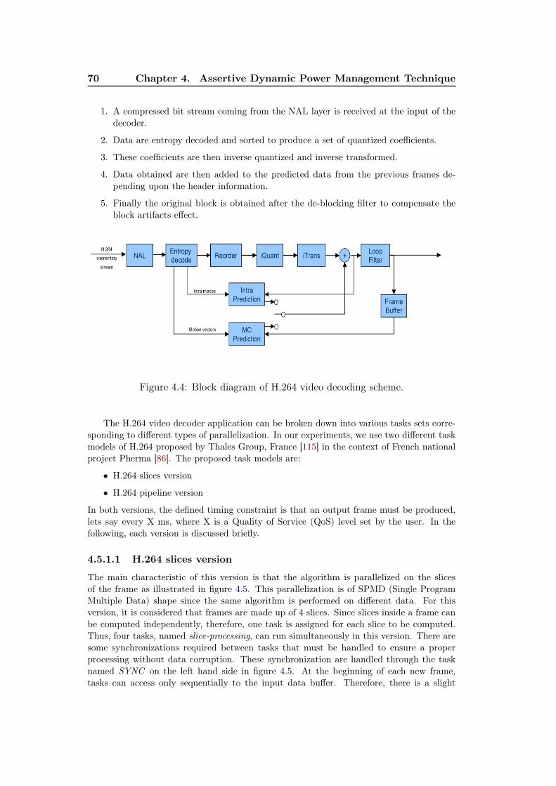
70 Chapter 4. Assertive Dynamic Power Management Technique
1. A compressed bit stream coming from the NAL layer is received at the input of thedecoder.
2. Data are entropy decoded and sorted to produce a set of quantized coefficients.
3. These coefficients are then inverse quantized and inverse transformed.
4. Data obtained are then added to the predicted data from the previous frames de-pending upon the header information.
5. Finally the original block is obtained after the de-blocking filter to compensate theblock artifacts effect.
Figure 4.4: Block diagram of H.264 video decoding scheme.
The H.264 video decoder application can be broken down into various tasks sets corre-sponding to different types of parallelization. In our experiments, we use two different taskmodels of H.264 proposed by Thales Group, France [115] in the context of French nationalproject Pherma [86]. The proposed task models are:
• H.264 slices version
• H.264 pipeline version
In both versions, the defined timing constraint is that an output frame must be produced,lets say every X ms, where X is a Quality of Service (QoS) level set by the user. In thefollowing, each version is discussed briefly.
4.5.1.1 H.264 slices version
The main characteristic of this version is that the algorithm is parallelized on the slicesof the frame as illustrated in figure 4.5. This parallelization is of SPMD (Single ProgramMultiple Data) shape since the same algorithm is performed on different data. For thisversion, it is considered that frames are made up of 4 slices. Since slices inside a frame canbe computed independently, therefore, one task is assigned for each slice to be computed.Thus, four tasks, named slice-processing, can run simultaneously in this version. There aresome synchronizations required between tasks that must be handled to ensure a properprocessing without data corruption. These synchronization are handled through the tasknamed SYNC on the left hand side in figure 4.5. At the beginning of each new frame,tasks can access only sequentially to the input data buffer. Therefore, there is a slight
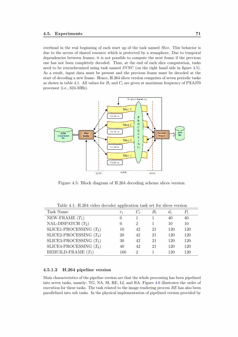
4.5. Experiments 71
overhead in the real beginning of each start up of the task named Slice. This behavior isdue to the access of shared resource which is protected by a semaphore. Due to temporaldependencies between frames, it is not possible to compute the next frame if the previousone has not been completely decoded. Thus, at the end of each slice computation, tasksneed to be resynchronized using task named SYNC (on the right hand side in figure 4.5).As a result, input data must be present and the previous frame must be decoded at thestart of decoding a new frame. Hence, H.264 slices version comprises of seven periodic tasksas shown in table 4.1. All values for Bi and Ci are given at maximum frequency of PXA270processor (i.e., 624-MHz).
Figure 4.5: Block diagram of H.264 decoding scheme slices version.
Table 4.1: H.264 video decoder application task set for slices versionTask Name ri Ci Bi di Pi
NEW-FRAME (T1) 0 1 1 40 40NAL-DISPATCH (T2) 0 2 1 10 10SLICE1-PROCESSING (T3) 10 42 21 120 120SLICE2-PROCESSING (T4) 20 42 21 120 120SLICE3-PROCESSING (T5) 30 42 21 120 120SLICE4-PROCESSING (T6) 40 42 21 120 120REBUILD-FRAME (T7) 160 2 1 120 120
4.5.1.2 H.264 pipeline version
Main characteristics of the pipeline version are that the whole processing has been pipelinedinto seven tasks, namely; TG, NA, SI, RE, LI, and RA. Figure 4.6 illustrates the order ofexecution for these tasks. The task related to the image rendering process RE has also beenparallelized into sub tasks. In the physical implementation of pipelined version provided by
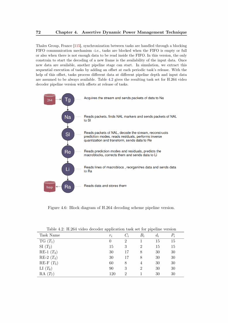
72 Chapter 4. Assertive Dynamic Power Management Technique
Thales Group, France [115], synchronization between tasks are handled through a blockingFIFO communication mechanism -i.e., tasks are blocked when the FIFO is empty or fullor also when there is not enough data to be read inside the FIFO. In this version, the onlyconstrain to start the decoding of a new frame is the availability of the input data. Oncenew data are available, another pipeline stage can start. In simulation, we extract thissequential execution of tasks by adding an offset at each periodic task’s release. With thehelp of this offset, tasks process different data at different pipeline depth and input dataare assumed to be always available. Table 4.2 gives the resulting task set for H.264 videodecoder pipeline version with offsets at release of tasks.
Figure 4.6: Block diagram of H.264 decoding scheme pipeline version.
Table 4.2: H.264 video decoder application task set for pipeline versionTask Name ri Ci Bi di Pi
TG (T1) 0 2 1 15 15SI (T2) 15 3 2 15 15RE-1 (T3) 30 17 8 30 30RE-2 (T4) 30 17 8 30 30RE-F (T5) 60 8 4 30 30LI (T6) 90 3 2 30 30RA (T7) 120 2 1 30 30
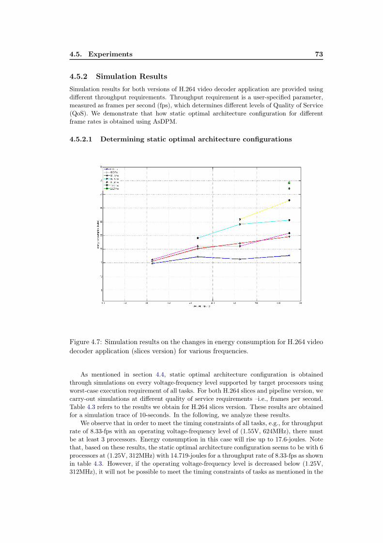
4.5. Experiments 73
4.5.2 Simulation Results
Simulation results for both versions of H.264 video decoder application are provided usingdifferent throughput requirements. Throughput requirement is a user-specified parameter,measured as frames per second (fps), which determines different levels of Quality of Service(QoS). We demonstrate that how static optimal architecture configuration for differentframe rates is obtained using AsDPM.
4.5.2.1 Determining static optimal architecture configurations
Figure 4.7: Simulation results on the changes in energy consumption for H.264 videodecoder application (slices version) for various frequencies.
As mentioned in section 4.4, static optimal architecture configuration is obtainedthrough simulations on every voltage-frequency level supported by target processors usingworst-case execution requirement of all tasks. For both H.264 slices and pipeline version, wecarry-out simulations at different quality of service requirements –i.e., frames per second.Table 4.3 refers to the results we obtain for H.264 slices version. These results are obtainedfor a simulation trace of 10-seconds. In the following, we analyze these results.
We observe that in order to meet the timing constraints of all tasks, e.g., for throughputrate of 8.33-fps with an operating voltage-frequency level of (1.55V, 624MHz), there mustbe at least 3 processors. Energy consumption in this case will rise up to 17.6-joules. Notethat, based on these results, the static optimal architecture configuration seems to be with 6
processors at (1.25V, 312MHz) with 14.719-joules for a throughput rate of 8.33-fps as shownin table 4.3. However, if the operating voltage-frequency level is decreased below (1.25V,312MHz), it will not be possible to meet the timing constraints of tasks as mentioned in the
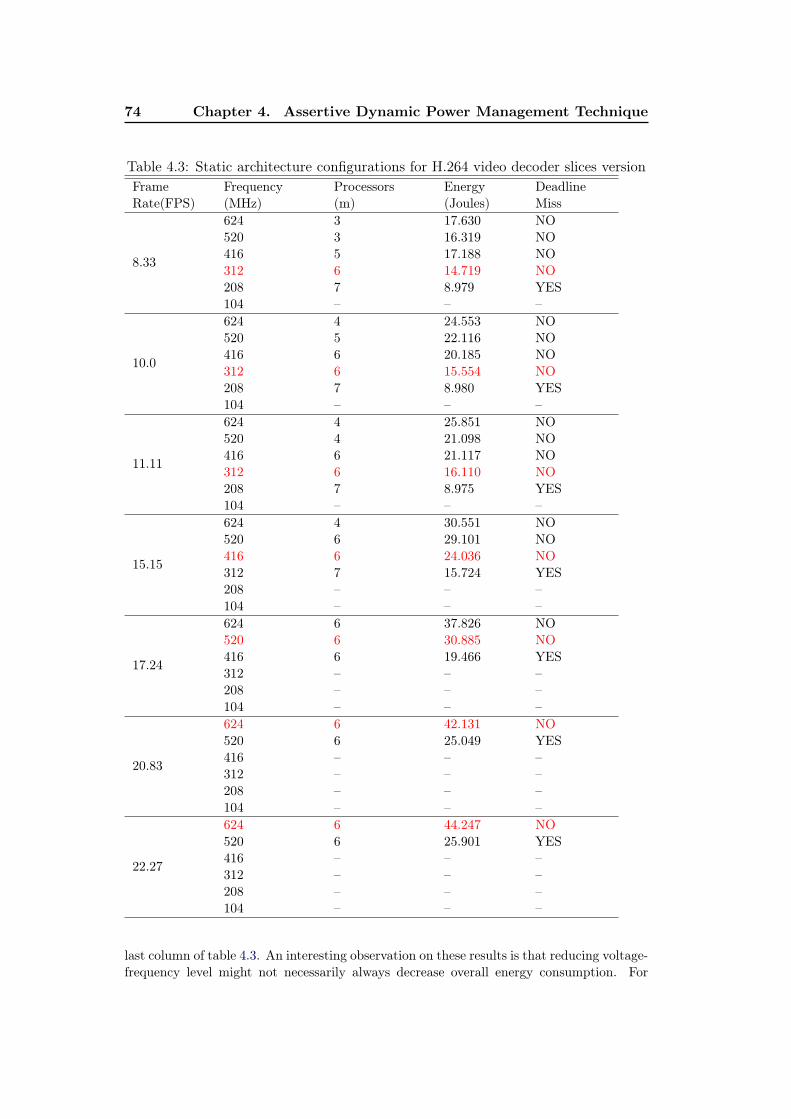
74 Chapter 4. Assertive Dynamic Power Management Technique
Table 4.3: Static architecture configurations for H.264 video decoder slices versionFrameRate(FPS)
Frequency(MHz)
Processors(m)
Energy(Joules)
DeadlineMiss
8.33
624 3 17.630 NO520 3 16.319 NO416 5 17.188 NO312 6 14.719 NO208 7 8.979 YES104 – – –
10.0
624 4 24.553 NO520 5 22.116 NO416 6 20.185 NO312 6 15.554 NO208 7 8.980 YES104 – – –
11.11
624 4 25.851 NO520 4 21.098 NO416 6 21.117 NO312 6 16.110 NO208 7 8.975 YES104 – – –
15.15
624 4 30.551 NO520 6 29.101 NO416 6 24.036 NO312 7 15.724 YES208 – – –104 – – –
17.24
624 6 37.826 NO520 6 30.885 NO416 6 19.466 YES312 – – –208 – – –104 – – –
20.83
624 6 42.131 NO520 6 25.049 YES416 – – –312 – – –208 – – –104 – – –
22.27
624 6 44.247 NO520 6 25.901 YES416 – – –312 – – –208 – – –104 – – –
last column of table 4.3. An interesting observation on these results is that reducing voltage-frequency level might not necessarily always decrease overall energy consumption. For

4.5. Experiments 75
Table 4.4: Static architecture configurations for H.264 video decoder pipeline versionFrameRate(FPS)
Frequency(MHz)
Processors(m)
Energy(Joules)
DeadlineMiss
10.0
624 1 9.204 NO520 1 6.716 NO416 2 6.458 NO312 2 5.349 NO208 6 7.362 NO104 5 2.703 YES
12.0
624 1 9.211 NO520 2 8.785 NO416 2 6.721 NO312 2 5.520 NO208 3 3.809 NO104 6 3.281 YES
15.0
624 1 9.224 NO520 2 9.600 NO416 2 8.514 NO312 3 7.611 NO208 5 6.317 NO104 6 3.301 YES
20.0
624 2 11.982 NO520 2 10.402 NO416 2 8.561 NO312 3 7.848 NO208 5 6.367 YES104 – – –
25.0
624 2 14.631 NO520 2 12.665 NO416 3 11.327 NO312 3 8.048 NO208 4 5.111 YES104 – – –
32.0
624 2 17.768 NO520 3 16.860 NO416 4 15.651 NO312 5 11.589 YES208 – – –104 – – –
instance, static architecture configuration at (1.45V, 520MHz) with 3 processors consumesless energy than (1.35V, 416MHz) with 5 processors. As a result, the increase in number ofprocessor must be followed by an sufficient decrease in the operating voltage-frequency level,otherwise, the overall energy consumption will not be lowered enough. For each throughputrequirement, the optimal configuration from the energy saving point of view is highlighted inred color in table 4.3. Note that an optimal or most suitable static architecture configurationdepends also on the available physical platform. Figure 4.7 graphically illustrates the resultspresented in table 4.3 for those frequencies only, for which no deadline is missed. Figure

76 Chapter 4. Assertive Dynamic Power Management Technique
4.7 illustrates that reducing operating frequency does not always result in a linear decreasein energy consumption.
Table 4.4 represents similar results on static architecture configurations for H.264pipeline version for different throughput rates. Note that with pipeline version (see ta-ble 4.2), the achievable throughput rate is up to 32-fps. Configurations highlighted in redcolor against each throughput requirement are the optimal configurations only from energyconsumption point of view. Figure 4.8 illustrates the difference in energy consumptionbetween a statically non-optimized EDF schedule and a statically optimized EDF sched-ule of H.264 video decoder application (slices version) using AsDPM. Similar results arepresented in figure 4.9 for pipeline version of H.264 video decoder application. Energy con-sumed under statically non-optimized EDF-based schedule refers to the energy consumptionat maximum voltage-frequency level –i.e., (1.55V, 624MHz), and m processors as requiredby the schedulability analysis of EDF for every QoS requirement.
The use of AsDPM for determining static optimal architecture configurations enablesthe designer to explore target architecture. Indeed, we have been able to test the timingconstraints of target application at different throughput requirements. Moreover, we havebeen able to identify what would be the minimum needs in terms of processing platformresources (i.e., number of processors and their corresponding operating voltage-frequencylevel) to fit different throughput requirements. If the end-user has an energy budget torespect, this technique helps him/her to have an energy forecast of the target configuration.
Table 4.5: Static optimal architecture configurations for H.264 video decoder slicesversion for different QoS requirements
Frame Rate(FPS)
Frequency(MHz)
Processors(m)
Energy(Joules)
8.33 312 6 14.71910.0 312 6 15.55411.11 312 6 16.11015.15 416 6 24.03617.24 520 6 30.88520.83 624 6 42.13122.27 624 6 44.247
Table 4.6: Static optimal architecture configurations for H.264 video decoderpipeline version for different QoS requirements
Frame Rate(FPS)
Frequency(MHz)
Processors(m)
Energy(Joules)
10.0 312 2 5.34912.0 208 3 3.80915.0 208 5 6.31720.0 312 3 7.84825.0 312 3 8.04832.0 416 4 15.651
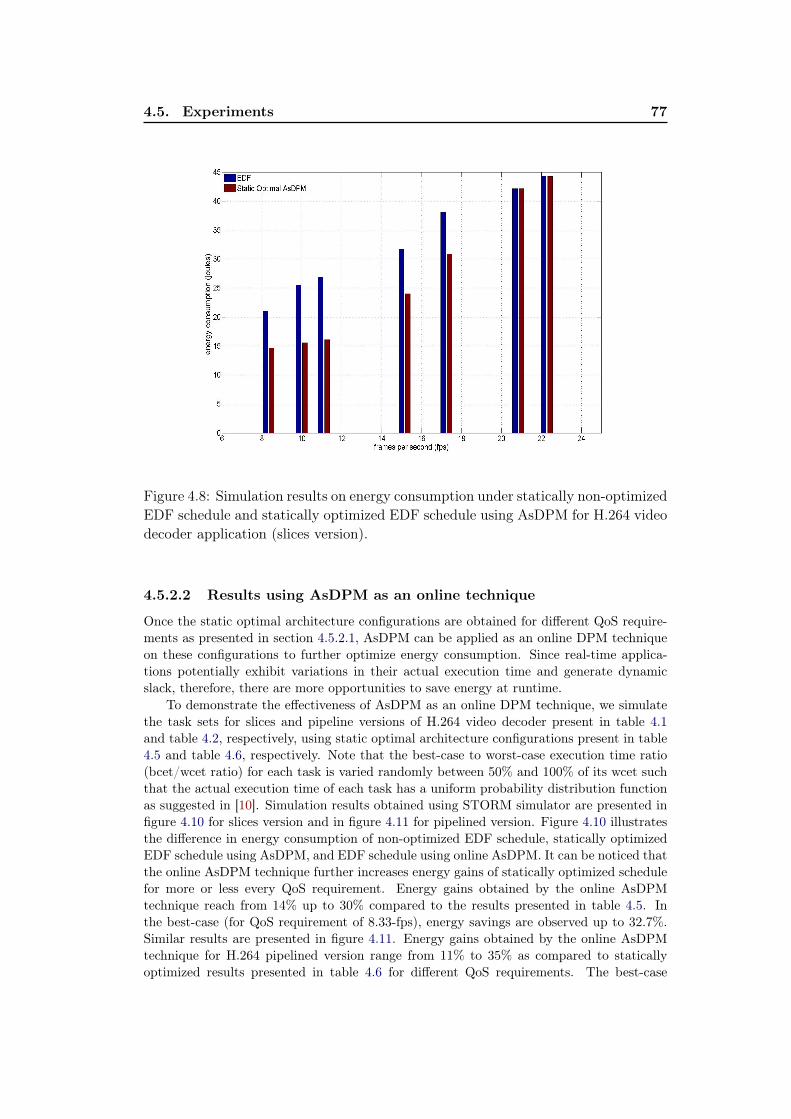
4.5. Experiments 77
Figure 4.8: Simulation results on energy consumption under statically non-optimizedEDF schedule and statically optimized EDF schedule using AsDPM for H.264 videodecoder application (slices version).
4.5.2.2 Results using AsDPM as an online technique
Once the static optimal architecture configurations are obtained for different QoS require-ments as presented in section 4.5.2.1, AsDPM can be applied as an online DPM techniqueon these configurations to further optimize energy consumption. Since real-time applica-tions potentially exhibit variations in their actual execution time and generate dynamicslack, therefore, there are more opportunities to save energy at runtime.
To demonstrate the effectiveness of AsDPM as an online DPM technique, we simulatethe task sets for slices and pipeline versions of H.264 video decoder present in table 4.1and table 4.2, respectively, using static optimal architecture configurations present in table4.5 and table 4.6, respectively. Note that the best-case to worst-case execution time ratio(bcet/wcet ratio) for each task is varied randomly between 50% and 100% of its wcet suchthat the actual execution time of each task has a uniform probability distribution functionas suggested in [10]. Simulation results obtained using STORM simulator are presented infigure 4.10 for slices version and in figure 4.11 for pipelined version. Figure 4.10 illustratesthe difference in energy consumption of non-optimized EDF schedule, statically optimizedEDF schedule using AsDPM, and EDF schedule using online AsDPM. It can be noticed thatthe online AsDPM technique further increases energy gains of statically optimized schedulefor more or less every QoS requirement. Energy gains obtained by the online AsDPMtechnique reach from 14% up to 30% compared to the results presented in table 4.5. Inthe best-case (for QoS requirement of 8.33-fps), energy savings are observed up to 32.7%.Similar results are presented in figure 4.11. Energy gains obtained by the online AsDPMtechnique for H.264 pipelined version range from 11% to 35% as compared to staticallyoptimized results presented in table 4.6 for different QoS requirements. The best-case

78 Chapter 4. Assertive Dynamic Power Management Technique
Figure 4.9: Simulation results on energy consumption under statically non-optimizedEDF schedule and statically optimized EDF schedule using AsDPM for H.264 videodecoder application (pipeline version).
energy savings in this case are observed up to 35.8% for QoS requirement of 15-fps.Note that the results provided on the percentage of energy gains while using the online
AsDPM technique are given as compared to the energy gains of statically optimized results.If no static optimizations are performed, achievable gains on energy using the online AsDPMtechnique alone would be significantly large as compared to the presented results.
4.5.3 Comparative Analysis of the AsDPM Technique
Although, many of the existing DPM techniques claim significant power and energy savingsfor real-time application models, producing the same results for such techniques in simula-tion settings other than the one used by authors is neither straightforward nor trivial. Thisis one of the limitations for us as well while comparing the performance of our proposedtechnique with existing techniques. Nevertheless, in order to give a reasonable idea on theperformance of our proposed technique, in this section, we provide a comparative analysisof energy savings under AsDPM and a theoretically ideal DPM technique. A theoreticallyideal DPM technique is the one that would have no temporal or energy penalty while tran-sitioning a processor to power-efficient states and it could transition a processor as soonas an idle time interval is detected. Moreover, all idle time intervals could be exploitedfor energy savings under such technique. Although, it is impossible to have zero penaltiesin existing processor technology, energy-efficiency of such an ideal DPM technique gives agood theoretical reference for measuring the performance of other techniques.
Figure 4.12 illustrates the results we obtain while comparing the energy savings undernon-optimized EDF schedule, static optimal AsDPM, online AsDPM, and ideal DPM for
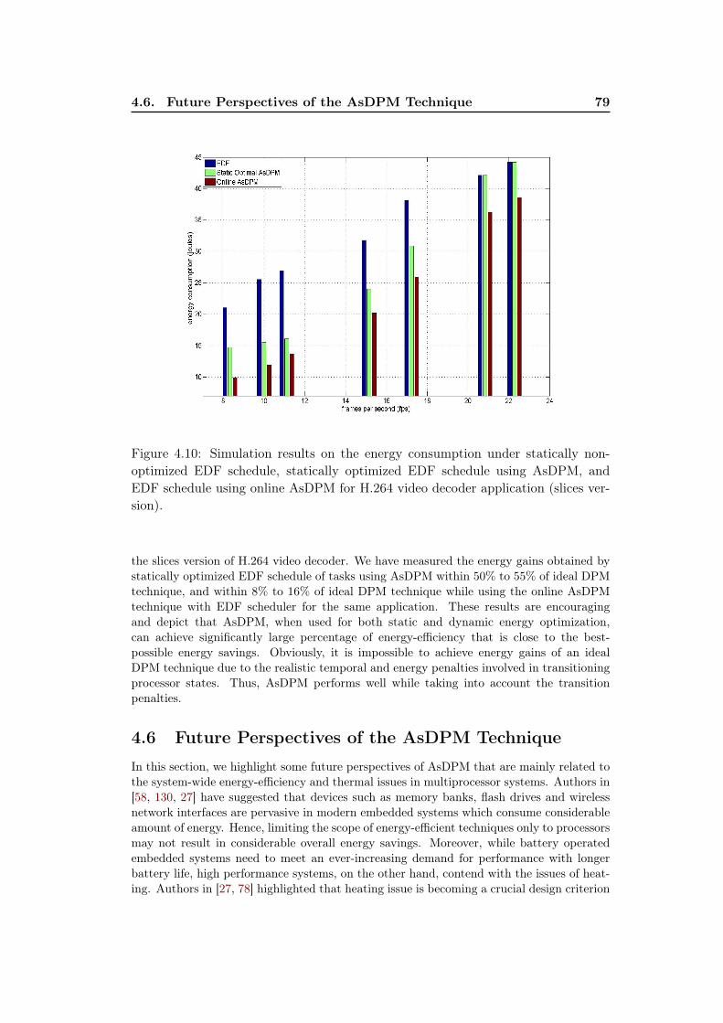
4.6. Future Perspectives of the AsDPM Technique 79
Figure 4.10: Simulation results on the energy consumption under statically non-optimized EDF schedule, statically optimized EDF schedule using AsDPM, andEDF schedule using online AsDPM for H.264 video decoder application (slices ver-sion).
the slices version of H.264 video decoder. We have measured the energy gains obtained bystatically optimized EDF schedule of tasks using AsDPM within 50% to 55% of ideal DPMtechnique, and within 8% to 16% of ideal DPM technique while using the online AsDPMtechnique with EDF scheduler for the same application. These results are encouragingand depict that AsDPM, when used for both static and dynamic energy optimization,can achieve significantly large percentage of energy-efficiency that is close to the best-possible energy savings. Obviously, it is impossible to achieve energy gains of an idealDPM technique due to the realistic temporal and energy penalties involved in transitioningprocessor states. Thus, AsDPM performs well while taking into account the transitionpenalties.
4.6 Future Perspectives of the AsDPM Technique
In this section, we highlight some future perspectives of AsDPM that are mainly related tothe system-wide energy-efficiency and thermal issues in multiprocessor systems. Authors in[58, 130, 27] have suggested that devices such as memory banks, flash drives and wirelessnetwork interfaces are pervasive in modern embedded systems which consume considerableamount of energy. Hence, limiting the scope of energy-efficient techniques only to processorsmay not result in considerable overall energy savings. Moreover, while battery operatedembedded systems need to meet an ever-increasing demand for performance with longerbattery life, high performance systems, on the other hand, contend with the issues of heat-ing. Authors in [27, 78] highlighted that heating issue is becoming a crucial design criterion

80 Chapter 4. Assertive Dynamic Power Management Technique
Figure 4.11: Simulation results on the energy consumption under statically non-optimized EDF schedule, statically optimized EDF schedule using AsDPM, andEDF schedule using online AsDPM for H.264 video decoder application (pipelineversion).
in order to ensure QoS requirements and limit the performance degradation for multi-coreand many-core systems with 2-dimensional and 3-dimensional chip manufacturing. In thissection, we briefly describe how AsDPM can be useful for other system components, es-pecially memory subsystem. Moreover, we describe how AsDPM confronts with heatingissue.
4.6.1 Memory Subsystem
Authors in [81] report that multi-banking in static and dynamic RAM-based main memoryarchitectures has been used as a popular method for reducing energy consumption. Inmulti-banking, memory space is divided into multiple banks, each of which can be controlledindependently of the others. One example of this type of memory architecture is RDRAM[93] in which each bank can work with four power-efficient states –i.e., active, standby, nap,and power-down. A memory bank can service a read/write request only in the active mode.If it is not servicing a memory request, it can be placed into one of aforementioned power-efficient state. Results reported by many researchers [31, 32, 41, 67, 82, 81] suggest thatsignificant reduction in energy consumption of memories is achieved through multi-bankingapproach. Authors in [81, 82] propose techniques based on clustering dynamically createddata with temporal affinity in the physical address space such that the data occupies asmall number of memory banks and remaining (unused) banks can be shutdown to saveleakage power. There is a trade off between energy saving and performance penalty (i.e.,resynchronization cost in terms of time and energy required to bring back a memory bank
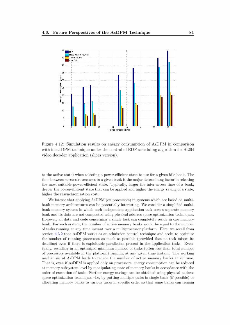
4.6. Future Perspectives of the AsDPM Technique 81
Figure 4.12: Simulation results on energy consumption of AsDPM in comparisonwith ideal DPM technique under the control of EDF scheduling algorithm for H.264video decoder application (slices version).
to the active state) when selecting a power-efficient state to use for a given idle bank. Thetime between successive accesses to a given bank is the major determining factor in selectingthe most suitable power-efficient state. Typically, larger the inter-access time of a bank,deeper the power-efficient state that can be applied and higher the energy saving of a state,higher the resynchronization cost.
We foresee that applying AsDPM (on processors) in systems which are based on multi-bank memory architectures can be potentially interesting. We consider a simplified multi-bank memory system in which each independent application task uses a separate memorybank and its data are not compacted using physical address space optimization techniques.However, all data and code concerning a single task can completely reside in one memorybank. For such system, the number of active memory banks would be equal to the numberof tasks running at any time instant over a multiprocessor platform. Here, we recall fromsection 4.3.2 that AsDPM works as an admission control technique and seeks to optimizethe number of running processors as much as possible (provided that no task misses itsdeadline) even if there is exploitable parallelism present in the application tasks. Even-tually, resulting in an optimized minimum number of tasks (often less than total numberof processors available in the platform) running at any given time instant. The workingmechanism of AsDPM leads to reduce the number of active memory banks at runtime.That is, even if AsDPM is applied only on processors, energy consumption can be reducedat memory subsystem level by manipulating state of memory banks in accordance with theorder of execution of tasks. Further energy savings can be obtained using physical addressspace optimization techniques –i.e, by putting multiple tasks in single bank (if possible) orallocating memory banks to various tasks in specific order so that some banks can remain

82 Chapter 4. Assertive Dynamic Power Management Technique
idle for longer duration.Only for illustration purpose, we consider a simulation trace obtained from STORM
simulator in which certain number of tasks are scheduled over three processors using globalEDF scheduling algorithm. Figure 4.13(a) illustrates the case when AsDPM is not applied.In this figure, it can be noticed that the number of banks being used at different time instantsvary quite frequently. Moreover, the number of state transitions is also significantly large.Whereas, in figure 4.13(b) which refers to the case when AsDPM is applied at processors,fewer than maximum number of memory banks are active most of the time and the numberof transitions is reduced as well. We did not carry out detailed experiments to validate thisobservation due to some limitations with the simulation tool. However, we feel confidentthat with larger application task sets, the gains on energy at memory subsystem level canbe capitalized.
4.6.2 Thermal Load Balancing
Authors in [27, 78] have highlighted that, due to the scaling-down of transistor, the avail-able chip surface for heat dissipation is reducing which results in increased power densities.Multiprocessor systems also behave as multiple heat sources which increase the likelihoodof temperature variations over shorter time and chip area rather than just a uniform tem-perature distribution over entire die.
In fact, in its actual state, AsDPM can potentially cause thermal imbalance on pro-cessors of the system. The source of (potential) thermal imbalance in the system is theworking principle of AsDPM, which seeks to minimize the number of running processors.That is, processors that are in running state are intended to be continuously running whileprocessors in power-efficient state are supposed to remain in their state as long as possible,resulting in increased temperature for the running processors and eventually reduce lifetime. To address this issue, we consider the thermal model of microprocessors presented byauthors in [73]. Authors state that, once the energy consumption of a processor is known,it can be used as an input for thermal model of processors. Using such a model, the tem-perature of processor can be estimated quite accurately. The temperature follows power,but does not change at once, rather it increases exponentially over time. The course ofprocessor’s temperature over time is modeled by authors in [73] through equation 4.5.
υ(t) =−C̃C2· e−C2t +
C1
C2· Pwr + υ0 (4.5)
Here, υ0 is the ambient temperature. C1 and C2 are constants depending on the thermalresistance and the thermal capacitance of processor and heat sink. C̃ is an integration con-stant depending on the initial temperature of processor. Equation 4.5 consists of a dynamicpart (first addend) and a static part (second and third addend). Static part depends onlyon the ambient temperature and power consumption of processor. It models the amountof temperature that a processor reaches after operating with constant power for long time.The dynamic part is an exponential function with time constant C2 and models the expo-nential rise or decay of a processor’s temperature after a change in power consumption. C2
can be determined by starting a computation-intensive task, which produces a maximum ofheat on a processor formerly idle, recording the temperature values over time, and fitting anexponential function to the experimental data. With knowledge of C2, the constant C1 canthen be determined from the static part of equation 4.5 by measuring temperature againstknown power consumption of the processor. Note that this thermal model does not takeinto account the physical placement of multiple cores which can potentially create thermalhot-spots.
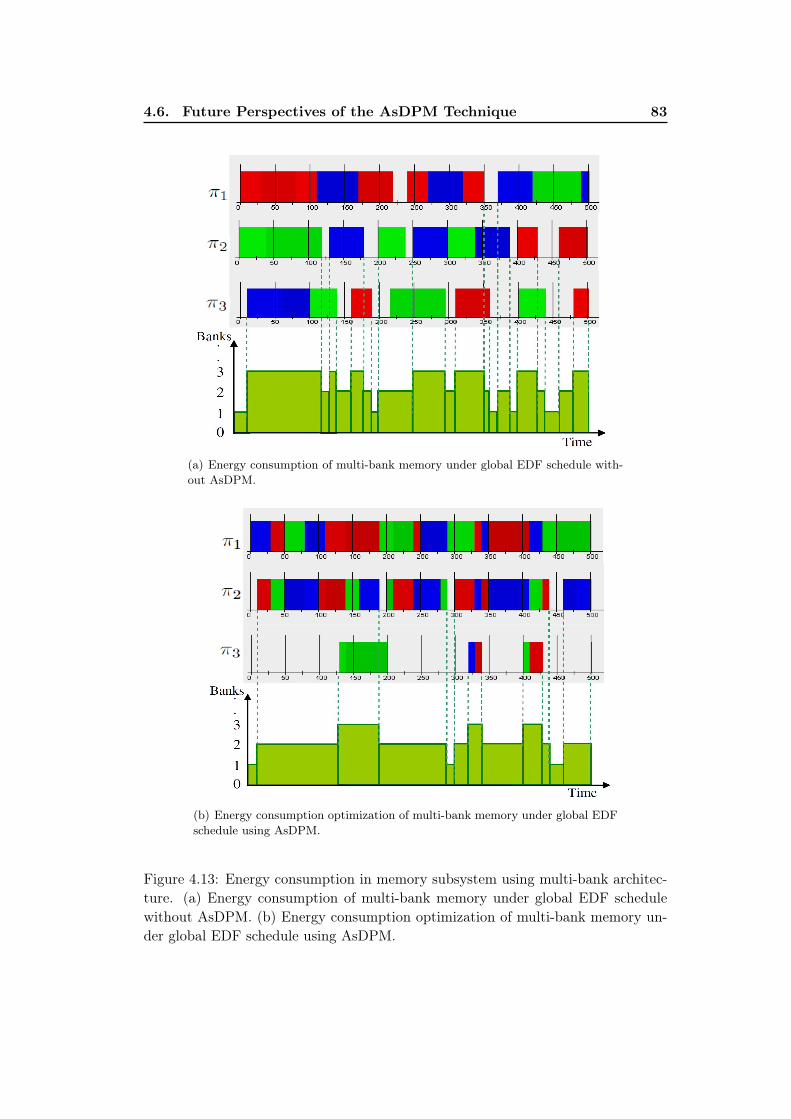
4.6. Future Perspectives of the AsDPM Technique 83
(a) Energy consumption of multi-bank memory under global EDF schedule with-out AsDPM.
(b) Energy consumption optimization of multi-bank memory under global EDFschedule using AsDPM.
Figure 4.13: Energy consumption in memory subsystem using multi-bank architec-ture. (a) Energy consumption of multi-bank memory under global EDF schedulewithout AsDPM. (b) Energy consumption optimization of multi-bank memory un-der global EDF schedule using AsDPM.
84 Chapter 4. Assertive Dynamic Power Management Technique
Equation 4.5 links the thermal variations of processor with the power consumptionvariations. Since power consumption can be estimated very precisely using many simula-tion tools, therefore, thermal variations of processor can be approximated using the modelpresented by [73]. The thermal imbalance in AsDPM can be dealt with using this modelby maintaining a power consumption profile, which could be approximated to temperaturevariations of processors, and evaluate this profile at suitable time instants, such as everyscheduling event. Based on the evolution of temperature over time, AsDPM can suggestthe controlling scheduler to replace the heated processors with relatively cooler proces-sors present in the platform at runtime. This could be a simple preventive measure tohomogenize temperature among all processors using only the power consumption modelsand scheduling decisions. However, more sophisticated approaches that deal with thermalimbalance can be used. This aspect still remains a future perspective of this dissertation.
4.7 Concluding Remarks
In this chapter, we have presented a new dynamic power management technique, called theAssertive Dynamic Power Management (AsDPM) technique, for multiprocessor real-timesystems. AsDPM is an admission control technique for real-time tasks which improvesenergy-efficiency of feasible task sets by deciding when exactly a ready task shall execute.Without this admission control, all ready tasks are executed as soon as there are enoughcomputing resources (processors) available in the system, leading to poor possibilities ofputting some processors in to power-efficient states. We have illustrated in this chapterthat although, AsDPM is an online dynamic power management technique, its workingprinciple can be used to determine static optimal architecture configurations (i.e., numberof processors and their corresponding voltage-frequency level required to meet real-timeconstraints in worst-case with reduced energy consumption) for target application throughsimulations, thus allowing static as well as dynamic power and energy optimization. Wehave provided experiments with H.264 video decoder application to support our proposi-tion. In the first step, we have demonstrated, through simulations, the use of the AsDPMtechnique for determining static optimal architecture configurations for H.264 video decoderapplication. In the second step, we have demonstrated the use of AsDPM as an online DPMtechnique which can further increase energy-efficiency of an already (statically) optimizedarchitecture configuration for any given application. For H.264 video decoder application,average achieved energy gains range from 14% to 35% depending on different QoS require-ments, while using AsDPM. Furthermore, we have briefly discussed the future perspectivesof the AsDPM technique, especially from the point of view of energy-efficiency at memorysubsystem level. We have briefly discussed heating issue in multiprocessor systems and pos-sible thermal load-balancing while using AsDPM. The AsDPM technique is also integratedin a hybrid power and energy management scheme which is presented in chapter 6.
Chapter 5
Deterministic Stretch-to-FitDVFS Technique
Contents5.1 Dynamic Voltage and Frequency Scaling . . . . . . . . . . . 85
5.2 Related Work . . . . . . . . . . . . . . . . . . . . . . . . . . . . 87
5.3 Deterministic Stretch-to-Fit Technique . . . . . . . . . . . . 90
5.3.1 Dynamic Slack Reclamation (DSR) Algorithm . . . . . . . . 90
5.3.2 Online Canonical Schedule . . . . . . . . . . . . . . . . . . . 93
5.3.3 Online Speculative speed adjustment Mechanism (OSM) . . . 97
5.3.4 m-Tasks Extension Technique (m-TE) . . . . . . . . . . . . . 98
5.4 Experiments . . . . . . . . . . . . . . . . . . . . . . . . . . . . 98
5.4.1 Setup . . . . . . . . . . . . . . . . . . . . . . . . . . . . . . . 99
5.4.2 Target Application . . . . . . . . . . . . . . . . . . . . . . . . 99
5.4.3 Simulation Results . . . . . . . . . . . . . . . . . . . . . . . . 99
5.5 Concluding Remarks . . . . . . . . . . . . . . . . . . . . . . . 104
5.1 Dynamic Voltage and Frequency Scaling
Dynamic voltage reduction is one of the effective techniques, which aim at changing energyconsumption profile of real-time embedded systems. This is because energy consumptionof processors is a quadratic function of supply voltage of processors [48] (see section 2.2.1).However, reduction in supply voltage also requires reduction in operating frequency, whichimplies a trade-off between energy consumption and system’s performance. Thanks to thesignificant evolution in processor-technology over the last few years, processors with vari-able voltages and frequencies are now available, thus allowing the design of highly flexiblesystems. Some examples of such processors are Marvell’s XScale R© technology-based em-bedded processors [72], Intel Speedstep [54], AMD PowerNow! [2], ARM [9], and TransmetaCrusoe [117]. In real-time systems that use variable voltage and frequency processors, choiceof voltage and frequency has direct impact on processor’s speed and consequently, on theordering and the execution of tasks. Thus, scheduling techniques and voltage/frequency se-lection mechanisms are tightly coupled and should be addressed together to ensure feasibilityof application tasks. In the last few years, Dynamic Voltage and Frequency Scaling(DVFS)techniques have emerged, which address the issue of energy-efficiency in real-time systemstogether with the scheduling. Real-time applications potentially exhibit variations in their

86 Chapter 5. Deterministic Stretch-to-Fit DVFS Technique
actual execution time and therefore, often finish earlier than their estimated worst-case exe-cution time [10, 40]. Real-time DVFS techniques exploit these variations in actual workloadin order to dynamically adjust voltage and frequency of processors to reduce their powerand energy consumption. However, one of the challenges for these techniques is to preservethe feasibility of schedule and provide deadline guarantees.
Real-time DVFS techniques are broadly classified into inter-task and intra-task strate-gies [79]. Inter-task DVFS techniques redistribute dynamic slack time either to all readytasks [51, 79] or to immediate priority single ready task only at task boundaries. That is,inter-task DVFS techniques make decisions related to slack reclamation only at schedulingevents referring to the termination of a job. On the other hand, in intra-task strategies,available (dynamic) slack time is reallocated inside the same task. These techniques oftenrequire insertion points in application’s code to measure its evolution over its executiontime. Some major drawbacks of intra-task scaling methods are that they require excessiveanalysis, runtime tracking and modification of the task source code, which is not alwaysfeasible in reality [76, 79, 98, 121]. Furthermore, they normally result in large number ofadditional voltage and frequency switching points and most of them assume continuous volt-age levels [96, 95]. In this chapter, we propose an inter-task dynamic voltage and frequencyscaling technique for real-time multiprocessor systems, called Deterministic Stretch-to-Fit(DSF) technique. The DSF technique comprises three algorithms, namely, Dynamic SlackReclamation (DSR) algorithm, Online Speculative speed adjustment Mechanism (OSM),and m-Tasks Extension (m-TE) algorithm. The DSR algorithm is the principle slack recla-mation algorithm of DSF that assigns dynamic slack, produced by a precedent task, to theappropriate priority next ready task that would execute on the same processor. While usingDSR, dynamic slack is not shared with other processors in the system. Rather, slack is fullyconsumed on the same processor by the task, to which it is once attributed. Such greedy al-location of slack allows the DSR algorithm to have large slowdown factor for scaling voltageand frequency for a single task, which eventually results in improved energy savings. DSRworks in conjunction with global scheduling algorithms on identical multiprocessor real-time systems. The OSM and the m-TE algorithms are extensions of the DSR algorithm.The OSM algorithm is an online, adaptive, and speculative speed adjustment mechanism,which anticipates early completion of tasks and performs aggressive slowdown on processorspeed. Apart from saving more energy as compared to the stand-alone DSR algorithm, thisspeculative speed adjustment mechanism also helps to avoid radical changes in operatingfrequency and supply voltage, which results in reduced peak power consumption, whichleads to an increase in battery life for portable embedded systems. The m-TE algorithmextends an already existing One-Task Extension (OTE) technique for single-processor sys-tems onto multiprocessor systems. The DSF technique is implemented in conjunction withthe EDF global scheduling algorithm.
The DSF technique is mainly intended for multiprocessor systems. Though, applyingit on single-processor systems is also possible and in fact, rather trivial due to absenceof migrating tasks. The DSF technique is generic in the sense that if a feasible schedulefor a real-time target application exists under worst-case workload using (optimal or non-optimal) global scheduling algorithms, then the same schedule can be reproduced (usingactual workload) with less power and energy consumption. Thus, DSF can work in con-junction with various scheduling algorithms. We illustrate that tasks meet their deadlinesif the speed of processors is reduced, due to dynamic slack reclamation, according to therules that we provide for the DSR algorithm. We achieve these objectives by exploiting onlythe online information of tasks. DSF is based on the principle of following the canonicalexecution of tasks at runtime –i.e., an offline or static optimal schedule in which all jobs
5.2. Related Work 87
of tasks exhibit their worst-case execution time. A track of the execution of all tasks instatic optimal schedule needs to be kept in order to follow it at runtime [10]. However,producing and keeping an entire canonical schedule offline is impractical in multiprocessorsystems due to a priori unknown assignment of preemptive and migrating tasks to proces-sors. Therefore, we propose a scheme to produce an online canonical schedule ahead ofpractical schedule, which mimics the canonical execution of tasks only for future m-tasks.This reduces scheduler’s overhead at runtime as well as makes DSF an adaptive technique.The DSF technique can work for different processor technologies supporting discrete as wellas continuous voltage and frequency scaling. Processors that are able to operate on (moreor less) continuous voltage and frequency spectrum are becoming a reality [10]. Therefore,we provide our solution for systems that support both discrete and continuous dynamicvoltage and frequency scaling.
In this chapter, we use the following notations from the literature on scheduling theoryand low-power techniques.
Canonical schedule (Scan) is a static optimal schedule in which each task instancepresents its worst-case workload under a given scheduling algorithm.
Practical schedule (Spra) is an online schedule in which each task instance presentsvariations to its worst-case workload. These variations are bounded by best-case (Bi) andworst-case (Ci) execution times of that task.
Dynamic slack (ε) refers to the amount of time spared by a task due to its earlycompletion. It is the difference between worst-case execution requirement and actualexecution time exhibited by a task at runtime. It can be known only when a taskterminates its running job.
Scaling factor (φ) refers to factor by which the worst-case execution time of a taskis scaled (increased or decreased). It is calculated based on the amount of available slack(ε) on a processor and it is bounded by the task’s deadline.
We assume that it is possible to vary supply voltage and operating frequency (alsoreferred as a tuple (Vdd, Fop) hereafter) on every processor independently and over a con-tinuous spectrum between defined lower and upper bounds. This assumption can be liftedfor processors offering only discrete operating frequencies by adapting to the nearest pos-sible operating frequency. The focus of this chapter in mainly on the online optimizationof power/energy consumption techniques. Thus, we do not consider static optimization of(Vdd, Fop)1. It is also assumed that statically specified optimum speed ϑmax and corre-sponding optimum (Vdd, Fop) are known a priori. Speed of a processor at any time instantis referred as ϑ and minimum allowable processor speed is referred as ϑmin such that (∀ϑ,ϑmin ≤ ϑ ≤ ϑmax).
5.2 Related Work
In this section, we provide the reader a review of the stat-of-the-art on existing real-timeDVFS techniques. Figure 5.1, which is adopted from [79] with slight modifications, gives aperspective of how the dynamic slack time is redistributed under different real-time DVFS
1The problem of static power optimization is briefly discussed in chapter 4

88 Chapter 5. Deterministic Stretch-to-Fit DVFS Technique
strategies. Figure 5.1 illustrates the evolution of processor’s frequency during the executionof a job Ti,j under different DVFS strategies. The worst-case execution time Ci,j of Ti,j isknown a priori. However, job Ti,j requires only AETi,j units of actual execution time tocomplete. Figure 5.1 (i) illustrates the case, in which Ti,j executes with maximum frequencyof processor, which is least effective from the point of view of energy consumption optimiza-tion. Figure 5.1 (ii) illustrates an ideal stretch strategy. An ideal stretch, however, is notfeasible in practice because it is not possible to know a priori the exact amount of actualexecution time of a task’s job. Thus, it is impossible to scale processor’s frequency with anideal scaling factor. Nevertheless, an ideal stretch strategy provides a good benchmark toassess a posteriori performance of other DVFS strategies. Figure 5.1 (iii) and (iv) illustratestochastic scheduling-based strategy and code instrumentation-based strategy, respectively.Both these strategies have opposite power consumption profiles. Indeed, the speed of pro-cessor increases with time in case of stochastic scheduling-based strategy (figure 5.1(iii)),while it decreases in case of code instrumentation-based strategy (figure 5.1(iv)) as theknowledge of remaining execution time becomes clearer. Figure 5.1 (v) illustrates the casein which dynamic slack time is distributed to all ready tasks. This technique results insmall values of scaling factor for frequency, which eventually results in insignificant gainson energy consumption. Figure 5.1 (vi) illustrates the case in which processor’s frequencyis reduced such that a tasks’s job finishes exactly at the same time instant, which was pre-viewed worst-case workload at maximum frequency. The idea to stretch a task’s executiontime to its worst-case boundary, as illustrated in figure 5.1(vi), is used in single-processorsystems. However, in multiprocessor systems, it is not trivial to apply simple stretchingdue to migrations and preemptions of jobs.
Figure 5.1: Dynamic slack redistribution of a task under various DVFS strategies.
Although real-time dynamic voltage and frequency scaling has become a major focus
5.2. Related Work 89
by real-time research community in recent years, its proposition stems back as early as in1994 when Weiser et al. first presented their work in [122]. Later on, numerous researchershave explored DVFS on single-processor systems such as [75, 98, 87, 10, 97, 122]. However,relatively few researchers have considered the problem of applying DVFS on multiprocessorplatforms such as [50, 99, 124]. A recent survey by Chen et al. [25] summarizes the state-of-art on energy-efficient scheduling for real-time systems on DVFS platforms, includingsingle-processor and multiprocessor systems.
For single processor systems, authors in [125] have proposed one of the earliest works,which presents an inter-task voltage scaling optimal algorithm to schedule a job set withspecified arrival times and deadlines on a continuous voltage processor. The analysis andcorrectness of this algorithm is based on EDF scheduler on a single processor system. Au-thors in [66] later extend the algorithm proposed by [125] to compute optimal slowdownfactors for the case of discrete voltage levels. Authors in [87, 10] have proposed inter-taskDVFS techniques using single-processor optimal scheduling algorithms such as EDF andFPP. In [87], authors have presented a cycle-conserving approach in which cumulative re-source utilization is recomputed at every scheduling event to rescale voltage and frequencyappropriately. This approach, however, distributes dynamic slack time to all ready taskswhich makes overall slowdown factor very small. Authors in [65] propose a power-awarescheduling technique using slack reclamation for systems with two voltage levels. Thus,limiting the number of scalable voltage levels to two. Authors in [75] have proposed andanalyzed several techniques for dynamic speed adjustment of processors with slack recla-mation. Authors in [91] propose an efficient heuristic technique to find the voltage scheduleof an FP real-time system –i.e., different voltage settings at different time for job instancesof aperiodic and periodic tasks.
In multiprocessor systems, the problem of energy minimization by dynamic slack recla-mation and dynamic speed adjustment for globally scheduled systems and independent taskmodel is considered in [129]. Authors in [129] consider dynamic slack sharing among mul-tiple processors and reducing the speed globally on all processors. This work is extendedin [128] to address the case of dependent tasks with AND/OR dependency constraints.Authors in [12] have proposed their solution for periodic hard real-time tasks on identicalmultiprocessors with DVS support when only partitioned scheduling is used. Authors in [12]adopt the EDF scheduling policy and investigate the joint effect of partitioning heuristicson the energy consumption and the feasibility. For systems with two-processors runningat two different but fixed voltage levels, authors in [124] proposed a two-phase schedul-ing scheme that minimizes energy consumption under the time constraints by choosingdifferent scheduling options determined at compile time. Authors in [10] have proposedan inter-task voltage scheduling solution for hard real-time systems comprised of a static(offline) solution to compute the optimal speed beforehand and an online solution basedon dynamic speed reduction mechanism. Authors in [127] highlight that processor energyoptimization solutions are not necessarily efficient from the perspective of whole system.They provide their solution for periodic and sporadic task models with a perspective ofsystem-wide energy-efficiency.
Apart from dynamic voltage and frequency scaling techniques for real-time multipro-cessor systems, some of the existing research work focuses on real-time static voltage andfrequency scaling as well [94, 46, 45]. The thesis for such work is based on the fact thatchanging voltage and frequency takes some time to ensure system synchronization due tophysical limitations. For instance, Intel Pentium M [49] processors require 10 − 15µs pervoltage and frequency scaling. It is possible to ignore the overhead in some cases. However,next-generation real-time systems are more rapid and controlled in faster control loops. For

90 Chapter 5. Deterministic Stretch-to-Fit DVFS Technique
such systems, frequent voltage and frequency scaling incurs significant overhead. Further-more, the optimal real-time scheduling algorithms for multiprocessors cause more frequentcontext switches than other algorithms. Thus, static voltage and frequency scaling is agood solution for these systems. One such solution is provided in [46]. Authors in [46] havehighlighted that, in currently available practical systems, optimal real-time static voltageand frequency scaling on multiprocessors is NP-hard partition problem since selectable pro-cessor frequency is discontinuous. Although static optimizations for voltage and frequencyare desirable, solutions based on only SVFS techniques are not good enough for systemsthat are likely to vary their configurations without system standstill. Moreover, systemswith aperiodic tasks would become sub-optimized online if the tasks’ arrival frequencyvaries. DVFS techniques are known to reduce dynamic power consumption (see section2.2.1). However, apart from latency issue related to changing voltage and frequency, DVFStechniques also cause increased leakage energy drain by lengthening the interval over whicha computation is carried out. As a solution, authors in [59] have proposed a leakage-awareDVFS technique for real-time systems in which, processor slowdown factors are computedbased on the critical speed for energy minimization. They have shown up to 5% gains usingcritical speed slowdown over a leakage oblivious DVFS solution.
The DSF technique is intended for periodic and independent tasks, which are scheduledover multiprocessor real-time systems. DSF is based on the idea of stretching the executiontime of a job, which consumes dynamic slack, to its worst-case boundary as illustrated infigure 5.1(vi). This stretching permits a hard real-time application to benefit from the sametimeliness guarantees as provided by worst-case schedulability analysis since the aggregateutilization of task set does not change due to processors’ frequency scaling.
5.3 Deterministic Stretch-to-Fit Technique
In this section, we present the algorithms proposed in the DSF technique –i.e., the DSRalgorithm, the OSM algorithm, and the m-TE algorithm.
5.3.1 Dynamic Slack Reclamation (DSR) Algorithm
Timeliness guarantees for real-time applications are provided through statically performedworst-case schedulability analysis. This, however, is a conservative analysis because atruntime, real-time tasks can exhibit large variations in their actual execution time andthereby produce dynamic slack due to their early completion [39]. The DSR algorithm isbased on detecting early completion of tasks. DSR determines the amount of dynamic slack(if any) by comparing the worst-case execution requirement of a task’s job with its actualexecution requirements. Since it is not possible to know a priori the exact amount of actualexecution requirement of a running task until it terminates, therefore, DSR computes theamount of dynamic slack at task boundaries only.
The DSR algorithm does not not share dynamic slack with other processors in thesystem. Rather, the slack is fully consumed on the same processor by a subsequent job,which is assigned to that processor. For instance, if a terminating job, let us say Ti−1,j ,produces positive dynamic slack time ε on a processor πk then the DSR algorithm, basedon the amount of available slack, determines a scaling factor φ for subsequently assignedappropriate priority job, let us say Ti,j , on πk. Scaling factor is calculated such that theconsumer task (i.e., task that consumes ε) finishes its slowed down execution by at most thesame time instant of its worst-case boundary as defined in the canonical schedule (Scan).An issue of concern in calculating φ is the knowledge of entire canonical schedule of tasks.
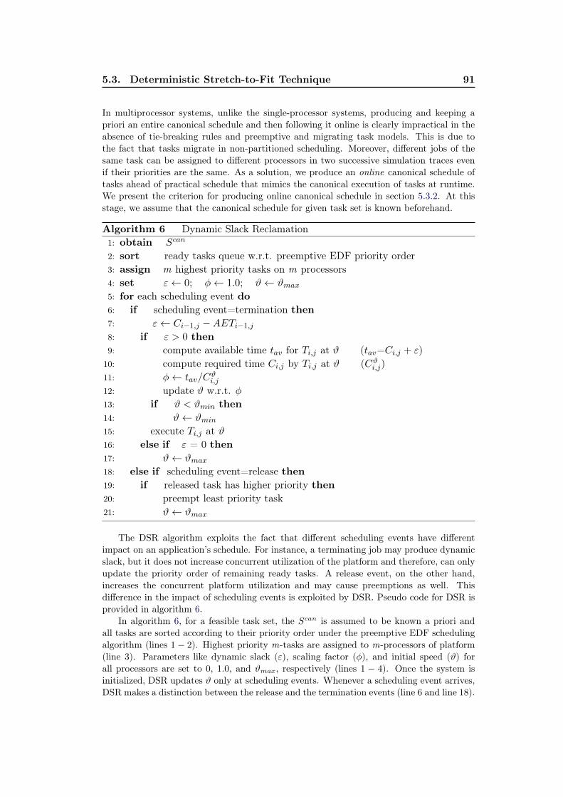
5.3. Deterministic Stretch-to-Fit Technique 91
In multiprocessor systems, unlike the single-processor systems, producing and keeping apriori an entire canonical schedule and then following it online is clearly impractical in theabsence of tie-breaking rules and preemptive and migrating task models. This is due tothe fact that tasks migrate in non-partitioned scheduling. Moreover, different jobs of thesame task can be assigned to different processors in two successive simulation traces evenif their priorities are the same. As a solution, we produce an online canonical schedule oftasks ahead of practical schedule that mimics the canonical execution of tasks at runtime.We present the criterion for producing online canonical schedule in section 5.3.2. At thisstage, we assume that the canonical schedule for given task set is known beforehand.
Algorithm 6 Dynamic Slack Reclamation1: obtain Scan
2: sort ready tasks queue w.r.t. preemptive EDF priority order3: assign m highest priority tasks on m processors4: set ε← 0; φ← 1.0; ϑ← ϑmax5: for each scheduling event do6: if scheduling event=termination then7: ε← Ci−1,j −AETi−1,j
8: if ε > 0 then9: compute available time tav for Ti,j at ϑ (tav=Ci,j + ε)
10: compute required time Ci,j by Ti,j at ϑ (Cϑi,j)11: φ← tav/C
ϑi,j
12: update ϑ w.r.t. φ13: if ϑ < ϑmin then14: ϑ← ϑmin15: execute Ti,j at ϑ16: else if ε = 0 then17: ϑ← ϑmax18: else if scheduling event=release then19: if released task has higher priority then20: preempt least priority task21: ϑ← ϑmax
The DSR algorithm exploits the fact that different scheduling events have differentimpact on an application’s schedule. For instance, a terminating job may produce dynamicslack, but it does not increase concurrent utilization of the platform and therefore, can onlyupdate the priority order of remaining ready tasks. A release event, on the other hand,increases the concurrent platform utilization and may cause preemptions as well. Thisdifference in the impact of scheduling events is exploited by DSR. Pseudo code for DSR isprovided in algorithm 6.
In algorithm 6, for a feasible task set, the Scan is assumed to be known a priori andall tasks are sorted according to their priority order under the preemptive EDF schedulingalgorithm (lines 1− 2). Highest priority m-tasks are assigned to m-processors of platform(line 3). Parameters like dynamic slack (ε), scaling factor (φ), and initial speed (ϑ) forall processors are set to 0, 1.0, and ϑmax, respectively (lines 1 − 4). Once the system isinitialized, DSR updates ϑ only at scheduling events. Whenever a scheduling event arrives,DSR makes a distinction between the release and the termination events (line 6 and line 18).

92 Chapter 5. Deterministic Stretch-to-Fit DVFS Technique
If a termination event is detected on a processor πk, DSR examines whether the completingjob (let us say Ti−1,j) has generated any positive dynamic slack (line 7). If dynamic slack isavailable (i.e., ε > 0) then the execution of subsequent appropriate priority job (let us sayTi,j) can be slowed down. To do so, the algorithm computes additional available time tavon πk at current processor speed ϑ. The worst-case execution time Cϑi,j of Ti,j is estimatedat ϑ that would have been required if πk continues to run at current speed ϑ (lines 8− 10).Once these two values are known, the scaling factor for Ti,j is computed and ϑ is updatedon πk accordingly (lines 11− 12). It is possible that the precedent job Ti−1,j has producedenough dynamic slack to reduce ϑ below the allowable minimum processor speed ϑmin. Toavoid such situation, ϑ is bounded by ϑmin in DSR (lines 13 − 15). If there is no positiveslack generated by Ti−1,j , processor πk continues to execute with maximum speed ϑmax(lines 16− 17).
If, on the other hand, a release event is detected on processor πk, DSR examines if thereleased job has its priority higher than the currently running m-tasks. If so, least priorityrunning job is preempted in order to run higher priority job and the speed of processoris set to maximum (lines 18 − 21). Note that when a higher priority task is released, theDSR algorithm increases the speed of processor to statically determined maximum (ϑmax)in order to respect the worst-case schedulability of released job. This is due to the factthat actual execution time of preempting task is unknown a priori. A speculative speedadjustment mechanism can be helpful in determining a probabilistic actual execution timethat would allow to keep the speed of processor less than ϑmax. Note that if the preemptedjob was executing with a speed other than ϑmax then its remaining execution time isalways restored w.r.t. maximum speed -i.e., ϑmax so that, upon resuming its execution, thepreempted job can always meet its deadline. In the following, we provide a simple exampleto elaborate the working of DSR. In this example, we provide an analytical view at firstand then support it with a simulation trace.
Example 5.1: Let us consider two real-time tasks, namely T1 and T2, which are scheduledunder the EDF scheduling algorithm. Figure 5.2 illustrates that T1 has higher priority overT2 due to smaller deadline. Let us consider that the job T1,j of T1 finishes its executionearlier than its worst-case execution requirement (C1,1) for its first job T1,1 as shown in inset(a). In the canonical schedule Scan –i.e., if job T1,1 would have finished with its worst-caseexecution time, the termination of T1,1 was estimated at time instant tcan1,1 . However, T1,1terminates at time instant tpra1,1 after consuming AET1,1 time units and produces ε units ofdynamic slack. Similarly, job T2,1 of T2 was expected to start its execution at time instanttcan1,1 and finish by tcan2,1 as illustrated in inset (b). However, due to the early completionof T1,1, now T2,1 has tav time units available (rather than C2,1 time units under worst-case) to finish its execution as expected in its Scan. Since AET2,1 is not known a priori,therefore, C2,1 is considered as the execution requirement for T2,1. Based on the knowledgeof available slack ε and task boundary in Scan (i.e., time instant tcan2,1 ), execution of T2,1 isslowed down by a factor of φ as shown in inset (c).
We simulate the same example using STORM simulator to validate the concept. Letus consider that the quadruplet values for T1 and T2 are (0, 6, 8, 8) and (0, 5, 20, 20), re-spectively. Let us consider that T1 has a best-case execution time of 3 time units andoften finishes earlier than its worst-case, whereas T2 always executes with its worst-caseexecution time. Figure 5.3(a) illustrates the canonical schedule of T1 and T2, in which bothtasks always consume their respective Ci time units at runtime. On the other hand, figure5.3(b) illustrates a practical schedule of the same tasks, in which T1 always finishes with itsbest-case execution time –i.e., 3 time units, and produces a dynamic slack of 3 time units(ε = 3). In figure 5.3(b) and figure 5.4, it is shown that task T2 consumes ε time units
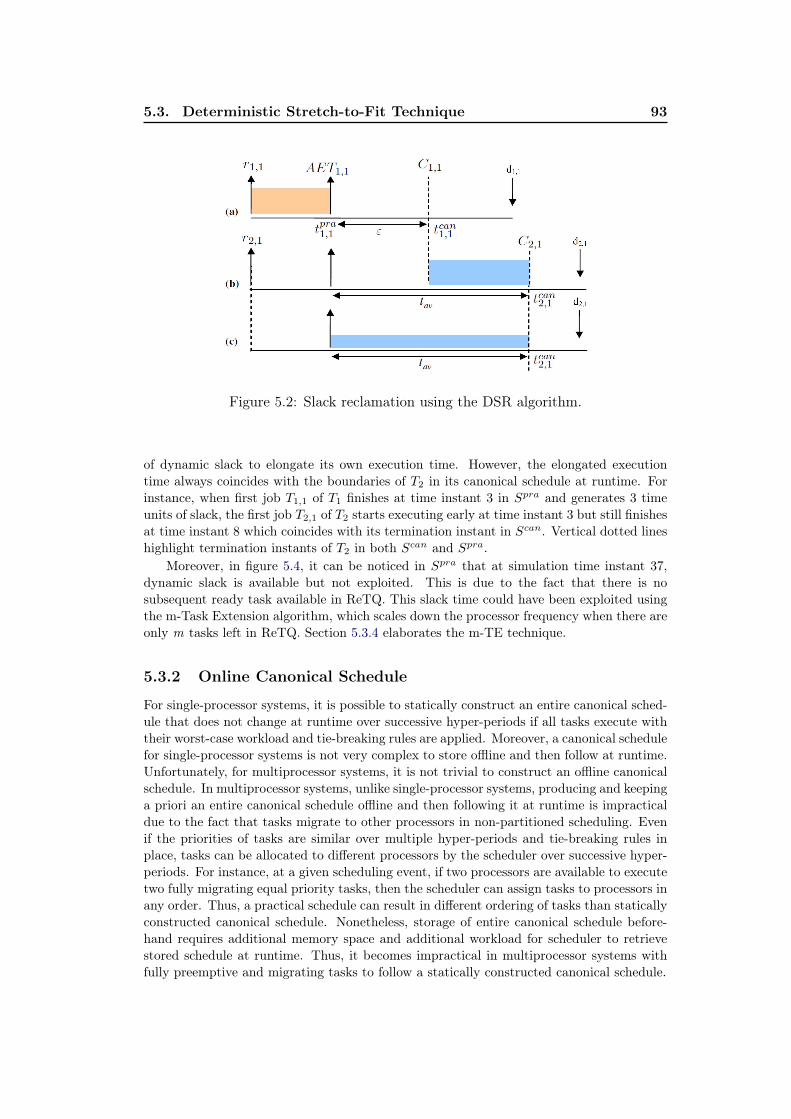
5.3. Deterministic Stretch-to-Fit Technique 93
Figure 5.2: Slack reclamation using the DSR algorithm.
of dynamic slack to elongate its own execution time. However, the elongated executiontime always coincides with the boundaries of T2 in its canonical schedule at runtime. Forinstance, when first job T1,1 of T1 finishes at time instant 3 in Spra and generates 3 timeunits of slack, the first job T2,1 of T2 starts executing early at time instant 3 but still finishesat time instant 8 which coincides with its termination instant in Scan. Vertical dotted lineshighlight termination instants of T2 in both Scan and Spra.
Moreover, in figure 5.4, it can be noticed in Spra that at simulation time instant 37,dynamic slack is available but not exploited. This is due to the fact that there is nosubsequent ready task available in ReTQ. This slack time could have been exploited usingthe m-Task Extension algorithm, which scales down the processor frequency when there areonly m tasks left in ReTQ. Section 5.3.4 elaborates the m-TE technique.
5.3.2 Online Canonical Schedule
For single-processor systems, it is possible to statically construct an entire canonical sched-ule that does not change at runtime over successive hyper-periods if all tasks execute withtheir worst-case workload and tie-breaking rules are applied. Moreover, a canonical schedulefor single-processor systems is not very complex to store offline and then follow at runtime.Unfortunately, for multiprocessor systems, it is not trivial to construct an offline canonicalschedule. In multiprocessor systems, unlike single-processor systems, producing and keepinga priori an entire canonical schedule offline and then following it at runtime is impracticaldue to the fact that tasks migrate to other processors in non-partitioned scheduling. Evenif the priorities of tasks are similar over multiple hyper-periods and tie-breaking rules inplace, tasks can be allocated to different processors by the scheduler over successive hyper-periods. For instance, at a given scheduling event, if two processors are available to executetwo fully migrating equal priority tasks, then the scheduler can assign tasks to processors inany order. Thus, a practical schedule can result in different ordering of tasks than staticallyconstructed canonical schedule. Nonetheless, storage of entire canonical schedule before-hand requires additional memory space and additional workload for scheduler to retrievestored schedule at runtime. Thus, it becomes impractical in multiprocessor systems withfully preemptive and migrating tasks to follow a statically constructed canonical schedule.
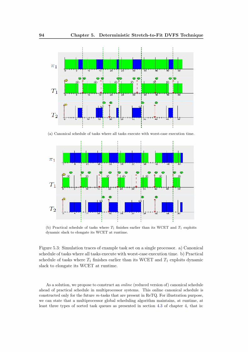
94 Chapter 5. Deterministic Stretch-to-Fit DVFS Technique
(a) Canonical schedule of tasks where all tasks execute with worst-case execution time.
(b) Practical schedule of tasks where T1 finishes earlier than its WCET and T1 exploitsdynamic slack to elongate its WCET at runtime.
Figure 5.3: Simulation traces of example task set on a single processor. a) Canonicalschedule of tasks where all tasks execute with worst-case execution time. b) Practicalschedule of tasks where T1 finishes earlier than its WCET and T1 exploits dynamicslack to elongate its WCET at runtime.
As a solution, we propose to construct an online (reduced version of) canonical scheduleahead of practical schedule in multiprocessor systems. This online canonical schedule isconstructed only for the future m-tasks that are present in ReTQ. For illustration purpose,we can state that a multiprocessor global scheduling algorithm maintains, at runtime, atleast three types of sorted task queues as presented in section 4.3 of chapter 4, that is:
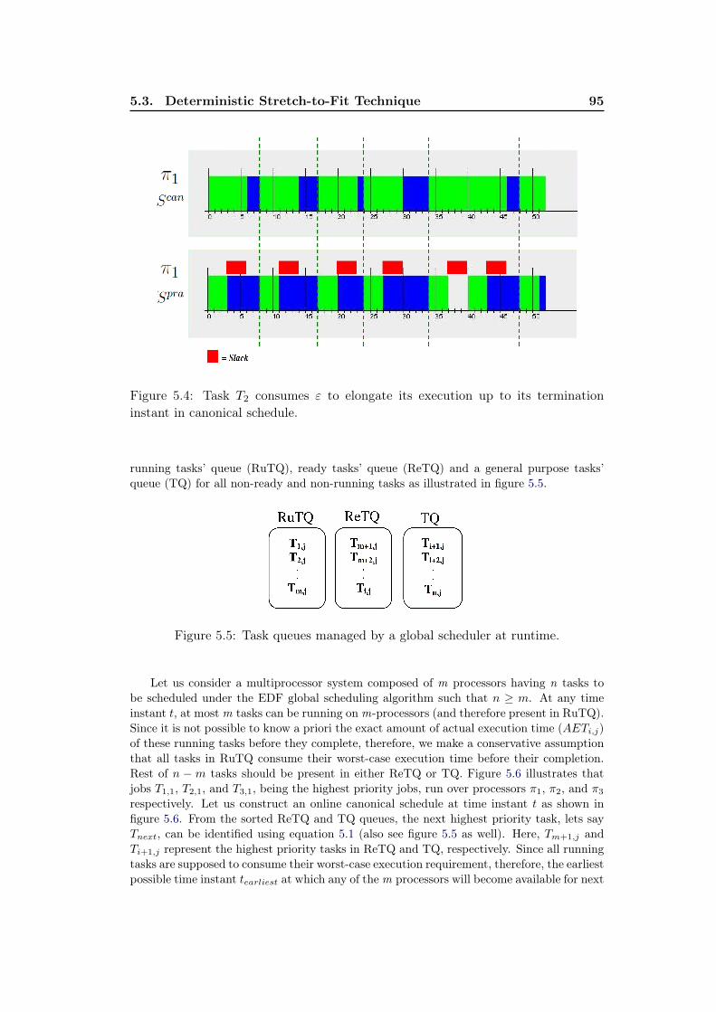
5.3. Deterministic Stretch-to-Fit Technique 95
Figure 5.4: Task T2 consumes ε to elongate its execution up to its terminationinstant in canonical schedule.
running tasks’ queue (RuTQ), ready tasks’ queue (ReTQ) and a general purpose tasks’queue (TQ) for all non-ready and non-running tasks as illustrated in figure 5.5.
Figure 5.5: Task queues managed by a global scheduler at runtime.
Let us consider a multiprocessor system composed of m processors having n tasks tobe scheduled under the EDF global scheduling algorithm such that n ≥ m. At any timeinstant t, at most m tasks can be running on m-processors (and therefore present in RuTQ).Since it is not possible to know a priori the exact amount of actual execution time (AETi,j)of these running tasks before they complete, therefore, we make a conservative assumptionthat all tasks in RuTQ consume their worst-case execution time before their completion.Rest of n −m tasks should be present in either ReTQ or TQ. Figure 5.6 illustrates thatjobs T1,1, T2,1, and T3,1, being the highest priority jobs, run over processors π1, π2, and π3respectively. Let us construct an online canonical schedule at time instant t as shown infigure 5.6. From the sorted ReTQ and TQ queues, the next highest priority task, lets sayTnext, can be identified using equation 5.1 (also see figure 5.5 as well). Here, Tm+1,j andTi+1,j represent the highest priority tasks in ReTQ and TQ, respectively. Since all runningtasks are supposed to consume their worst-case execution requirement, therefore, the earliestpossible time instant tearliest at which any of the m processors will become available for next
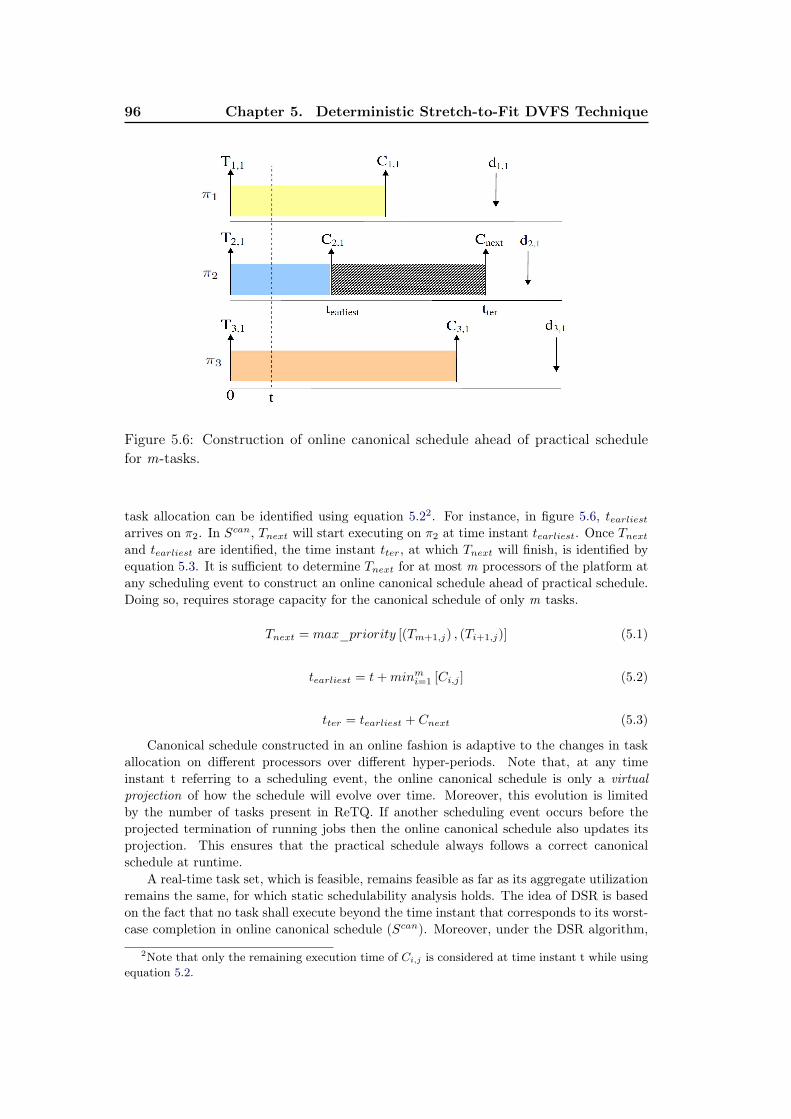
96 Chapter 5. Deterministic Stretch-to-Fit DVFS Technique
Figure 5.6: Construction of online canonical schedule ahead of practical schedulefor m-tasks.
task allocation can be identified using equation 5.22. For instance, in figure 5.6, tearliestarrives on π2. In Scan, Tnext will start executing on π2 at time instant tearliest. Once Tnextand tearliest are identified, the time instant tter, at which Tnext will finish, is identified byequation 5.3. It is sufficient to determine Tnext for at most m processors of the platform atany scheduling event to construct an online canonical schedule ahead of practical schedule.Doing so, requires storage capacity for the canonical schedule of only m tasks.
Tnext = max_priority [(Tm+1,j) , (Ti+1,j)] (5.1)
tearliest = t+minmi=1 [Ci,j ] (5.2)
tter = tearliest + Cnext (5.3)
Canonical schedule constructed in an online fashion is adaptive to the changes in taskallocation on different processors over different hyper-periods. Note that, at any timeinstant t referring to a scheduling event, the online canonical schedule is only a virtualprojection of how the schedule will evolve over time. Moreover, this evolution is limitedby the number of tasks present in ReTQ. If another scheduling event occurs before theprojected termination of running jobs then the online canonical schedule also updates itsprojection. This ensures that the practical schedule always follows a correct canonicalschedule at runtime.
A real-time task set, which is feasible, remains feasible as far as its aggregate utilizationremains the same, for which static schedulability analysis holds. The idea of DSR is basedon the fact that no task shall execute beyond the time instant that corresponds to its worst-case completion in online canonical schedule (Scan). Moreover, under the DSR algorithm,
2Note that only the remaining execution time of Ci,j is considered at time instant t while usingequation 5.2.
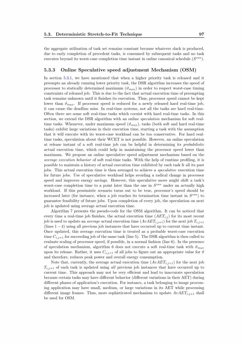
5.3. Deterministic Stretch-to-Fit Technique 97
the aggregate utilization of task set remains constant because whatever slack is produced,due to early completion of precedent tasks, is consumed by subsequent tasks and no taskexecutes beyond its worst-case completion time instant in online canonical schedule (Scan).
5.3.3 Online Speculative speed adjustment Mechanism (OSM)
In section 5.3.1, we have mentioned that when a higher priority task is released and itpreempts an already running lower priority task, the DSR algorithm increases the speed ofprocessor to statically determined maximum (ϑmax) in order to respect worst-case timingconstraints of released job. This is due to the fact that actual execution time of preemptingtask remains unknown until it finishes its execution. Thus, processor speed cannot be keptlower than ϑmax. If processor speed is reduced for a newly released hard real-time job,it can cause the deadline miss. In real-time systems, not all the tasks are hard real-time.Often there are some soft real-time tasks which coexist with hard real-time tasks. In thissection, we extend the DSR algorithm with an online speculation mechanism for soft real-time tasks. Whenever, under maximum speed (ϑmax), tasks (both soft and hard real-timetasks) exhibit large variations in their execution time, starting a task with the assumptionthat it will execute with its worst-case workload can be too conservative. For hard real-time tasks, speculation about their WCET is not possible. However, an online speculationat release instant of a soft real-time job can be helpful in determining its probabilisticactual execution time, which could help in maintaining the processor speed lower thanmaximum. We propose an online speculative speed adjustment mechanism based on theaverage execution behavior of soft real-time tasks. With the help of runtime profiling, it ispossible to maintain a history of actual execution time exhibited by each task fr all its pastjobs. This actual execution time is then averaged to achieve a speculative execution timefor future jobs. Use of speculative workload helps avoiding a radical change in processorspeed and improves energy savings. However, this speculative move might shift a task’sworst-case completion time to a point later than the one in Scan under an actually highworkload. If this pessimistic scenario turns out to be true, processor’s speed should beincreased later (for instance, when a job reaches its termination time instant in Scan) toguarantee feasibility of future jobs. Upon completion of every job, the speculation on nextjob is updated using average actual execution time.
Algorithm 7 presents the pseudo-code for the OSM algorithm. It can be noticed thatevery time a real-time job finishes, the actual execution time (AETi,j) for its most recentjob is used to update an average actual execution time (AvAETi,j+1) for the next job Ti,j+1
(lines 1− 4) using all previous job instances that have occurred up to current time instant.Once updated, this average execution time is treated as a probable worst-case executiontime Ci,j+1 for succeeding job of the same task (line 5). The DSR algorithm is then called toevaluate scaling of processor speed, if possible, in a normal fashion (line 6). In the presenceof speculation mechanism, algorithm 6 does not execute a soft real-time task with ϑmaxupon its release. Rather, it uses Ci,j+1 of all jobs to figure out an appropriate value for ϑand therefore, reduces peak power and overall energy consumption.
Note that, currently, the average actual execution time (AvAETi,j+1) for the next jobTi,j+1 of each task is updated using all previous job instances that have occurred up tocurrent time. This approach may not be very efficient and lead to inaccurate speculationbecause certain tasks may have different behavior (different variations in their AET) duringdifferent phases of application’s execution. For instance, a task belonging to image process-ing application may have small, medium, or large variations in its AET while processingdifferent image frames. Thus, more sophisticated mechanism to update AvAETi,j+1 shallbe used for OSM.
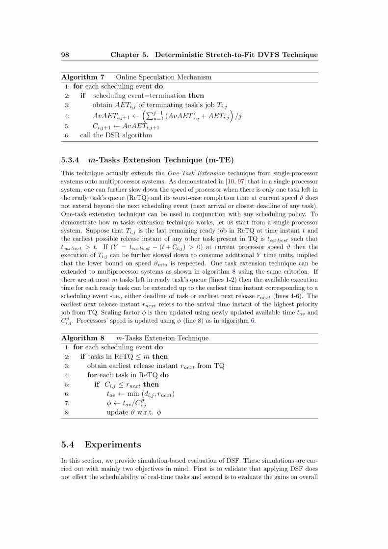
98 Chapter 5. Deterministic Stretch-to-Fit DVFS Technique
Algorithm 7 Online Speculation Mechanism1: for each scheduling event do2: if scheduling event=termination then3: obtain AETi,j of terminating task’s job Ti,j4: AvAETi,j+1 ←
(∑j−1u=1 (AvAET )u +AETi,j
)/j
5: Ci,j+1 ← AvAETi,j+1
6: call the DSR algorithm
5.3.4 m-Tasks Extension Technique (m-TE)
This technique actually extends the One-Task Extension technique from single-processorsystems onto multiprocessor systems. As demonstrated in [10, 97] that in a single processorsystem, one can further slow down the speed of processor when there is only one task left inthe ready task’s queue (ReTQ) and its worst-case completion time at current speed ϑ doesnot extend beyond the next scheduling event (next arrival or closest deadline of any task).One-task extension technique can be used in conjunction with any scheduling policy. Todemonstrate how m-tasks extension technique works, let us start from a single-processorsystem. Suppose that Ti,j is the last remaining ready job in ReTQ at time instant t andthe earliest possible release instant of any other task present in TQ is tearliest such thattearliest > t. If (Y = tearliest − (t+ Ci,j) > 0) at current processor speed ϑ then theexecution of Ti,j can be further slowed down to consume additional Y time units, impliedthat the lower bound on speed ϑmin is respected. One task extension technique can beextended to multiprocessor systems as shown in algorithm 8 using the same criterion. Ifthere are at most m tasks left in ready task’s queue (lines 1-2) then the available executiontime for each ready task can be extended up to the earliest time instant corresponding to ascheduling event -i.e., either deadline of task or earliest next release rnext (lines 4-6). Theearliest next release instant rnext refers to the arrival time instant of the highest priorityjob from TQ. Scaling factor φ is then updated using newly updated available time tav andCϑi,j . Processors’ speed is updated using φ (line 8) as in algorithm 6.
Algorithm 8 m-Tasks Extension Technique1: for each scheduling event do2: if tasks in ReTQ ≤ m then3: obtain earliest release instant rnext from TQ4: for each task in ReTQ do5: if Ci,j ≤ rnext then6: tav ← min (di,j , rnext)
7: φ ← tav/Cϑi,j
8: update ϑ w.r.t. φ
5.4 Experiments
In this section, we provide simulation-based evaluation of DSF. These simulations are car-ried out with mainly two objectives in mind. First is to validate that applying DSF doesnot effect the schedulability of real-time tasks and second is to evaluate the gains on overall
5.4. Experiments 99
energy savings of the system.
5.4.1 Setup
We evaluate the performance of DSF using STORM simulator [108]. We consider the samesystem model –i.e., task model, processing platform, and power and energy models, aspresented in chapter 2. One of the difference w.r.t. system model presented in chapter 2is that, we assume that it is possible to vary supply voltage and operating frequency (Vdd,Fop) on every processor independently and over a continuous spectrum between definedlower and upper bounds. This assumption can be lifted for processors that offer only afinite number of discrete operating frequencies. As suggested in [22], if the desired optimalspeed (corresponding to the achievable scalability of voltage/frequency) is not available on aprocessor, it has to be approximated with one of the existing values. To prevent any deadlinemiss, the processor speed should be set equal to the closest discrete level higher than theoptimal speed. This solution, however, may cause a waste of computational capacity and,consequently, of energy, especially when the choice for available operating frequencies islimited.
The EDF scheduling algorithm is used in the evaluation of DSF.
5.4.2 Target Application
The H.264 video decoder application is taken as main use case target application for eval-uating DSF. The main steps of the H.264 decoding process are depicted in figure 4.4 ofsection 4.5.1. In simulations related to the DSF technique, we use both versions (i.e., slicesand pipeline versions) of H.264 video decoder application as presented in chapter 4.
5.4.3 Simulation Results
We provide simulation results for both versions of H.264 video decoder application usingdifferent throughput requirements. Recall that throughput requirement is a user-specifiedparameter, measured as frames per second (fps), which determines different levels of Qualityof Service (QoS) for the H.264 application. The number of processors corresponding todifferent QoS (fps) requirement at maximum operating voltage and frequency level arealready determined (see table 5.1) using AsDPM presented in section 4.4 (see chapter 4).Performance of the DSF technique is analyzed based on energy consumption compared tonon-optimized case while using DSR lone, both DSR and OSM together, and using allthree algorithms together –i.e., DSR, OSM, and m-TE. Furthermore, we have comparedour results with two existing DVFS algorithms. Details are presented in section 5.4.3.4.
5.4.3.1 Simulation results of H.264 slices version
We simulate the task model presented in table 4.1 under the simulation settings provided intable 5.1. The bcet/wcet ratio is varied between 50% and 100% of wcet of tasks such thatAET of all tasks has a uniform probability distribution function as suggested in [10]. Fordifferent frame rates, we obtain results as illustrated in figure 5.7. These results representthe average energy consumption over three complete frames (i.e., hyper-periods). In figure5.7, it can be noticed that energy gains of the DSF technique, while using all its algorithmsin different combinations, result from 12% to 35% as compared to the non-optimizaedenergy consumption under EDF schedule. In the best-case, energy gains reach upto 45%,which reduces energy consumed per frame to 1.5J/frame as compared to 2.45J/frame in
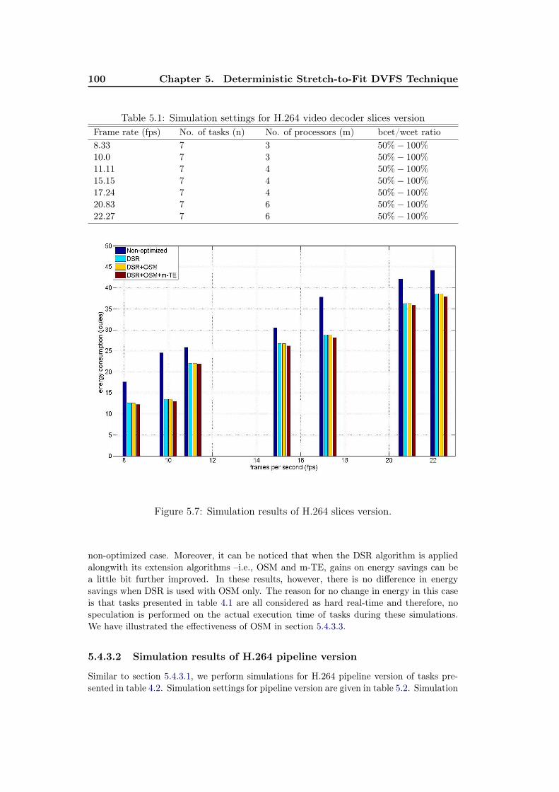
100 Chapter 5. Deterministic Stretch-to-Fit DVFS Technique
Table 5.1: Simulation settings for H.264 video decoder slices versionFrame rate (fps) No. of tasks (n) No. of processors (m) bcet/wcet ratio8.33 7 3 50%− 100%
10.0 7 3 50%− 100%
11.11 7 4 50%− 100%
15.15 7 4 50%− 100%
17.24 7 4 50%− 100%
20.83 7 6 50%− 100%
22.27 7 6 50%− 100%
Figure 5.7: Simulation results of H.264 slices version.
non-optimized case. Moreover, it can be noticed that when the DSR algorithm is appliedalongwith its extension algorithms –i.e., OSM and m-TE, gains on energy savings can bea little bit further improved. In these results, however, there is no difference in energysavings when DSR is used with OSM only. The reason for no change in energy in this caseis that tasks presented in table 4.1 are all considered as hard real-time and therefore, nospeculation is performed on the actual execution time of tasks during these simulations.We have illustrated the effectiveness of OSM in section 5.4.3.3.
5.4.3.2 Simulation results of H.264 pipeline version
Similar to section 5.4.3.1, we perform simulations for H.264 pipeline version of tasks pre-sented in table 4.2. Simulation settings for pipeline version are given in table 5.2. Simulation
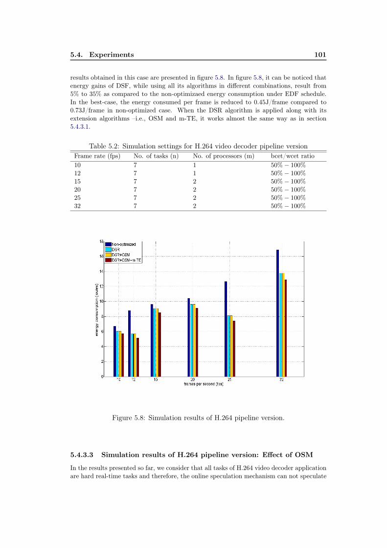
5.4. Experiments 101
results obtained in this case are presented in figure 5.8. In figure 5.8, it can be noticed thatenergy gains of DSF, while using all its algorithms in different combinations, result from5% to 35% as compared to the non-optimizaed energy consumption under EDF schedule.In the best-case, the energy consumed per frame is reduced to 0.45J/frame compared to0.73J/frame in non-optimized case. When the DSR algorithm is applied along with itsextension algorithms –i.e., OSM and m-TE, it works almost the same way as in section5.4.3.1.
Table 5.2: Simulation settings for H.264 video decoder pipeline versionFrame rate (fps) No. of tasks (n) No. of processors (m) bcet/wcet ratio10 7 1 50%− 100%
12 7 1 50%− 100%
15 7 2 50%− 100%
20 7 2 50%− 100%
25 7 2 50%− 100%
32 7 2 50%− 100%
Figure 5.8: Simulation results of H.264 pipeline version.
5.4.3.3 Simulation results of H.264 pipeline version: Effect of OSM
In the results presented so far, we consider that all tasks of H.264 video decoder applicationare hard real-time tasks and therefore, the online speculation mechanism can not speculate
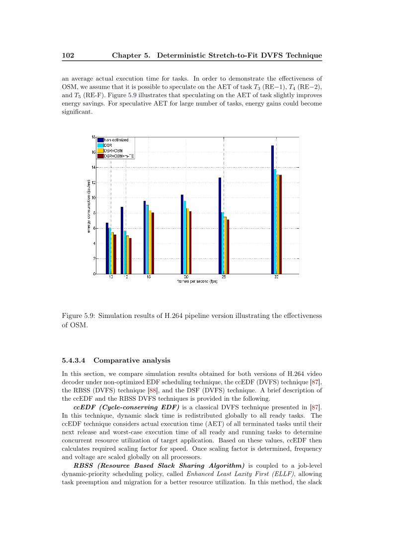
102 Chapter 5. Deterministic Stretch-to-Fit DVFS Technique
an average actual execution time for tasks. In order to demonstrate the effectiveness ofOSM, we assume that it is possible to speculate on the AET of task T3 (RE−1), T4 (RE−2),and T5 (RE-F). Figure 5.9 illustrates that speculating on the AET of task slightly improvesenergy savings. For speculative AET for large number of tasks, energy gains could becomesignificant.
Figure 5.9: Simulation results of H.264 pipeline version illustrating the effectivenessof OSM.
5.4.3.4 Comparative analysis
In this section, we compare simulation results obtained for both versions of H.264 videodecoder under non-optimized EDF scheduling technique, the ccEDF (DVFS) technique [87],the RBSS (DVFS) technique [88], and the DSF (DVFS) technique. A brief description ofthe ccEDF and the RBSS DVFS techniques is provided in the following.
ccEDF (Cycle-conserving EDF) is a classical DVFS technique presented in [87].In this technique, dynamic slack time is redistributed globally to all ready tasks. TheccEDF technique considers actual execution time (AET) of all terminated tasks until theirnext release and worst-case execution time of all ready and running tasks to determineconcurrent resource utilization of target application. Based on these values, ccEDF thencalculates required scaling factor for speed. Once scaling factor is determined, frequencyand voltage are scaled globally on all processors.
RBSS (Resource Based Slack Sharing Algorithm) is coupled to a job-leveldynamic-priority scheduling policy, called Enhanced Least Laxity First (ELLF), allowingtask preemption and migration for a better resource utilization. In this method, the slack
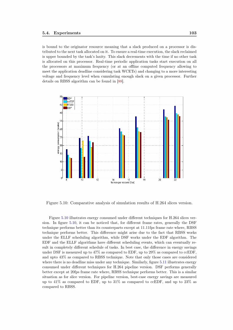
5.4. Experiments 103
is bound to the originator resource meaning that a slack produced on a processor is dis-tributed to the next task allocated on it. To ensure a real-time execution, the slack reclaimedis upper bounded by the task’s laxity. This slack decrements with the time if no other taskis allocated on this processor. Real-time periodic application tasks start execution on allthe processors at maximum frequency (or at an offline computed frequency allowing tomeet the application deadline considering task WCETs) and changing to a more interestingvoltage and frequency level when cumulating enough slack on a given processor. Furtherdetails on RBSS algorithm can be found in [88].
Figure 5.10: Comparative analysis of simulation results of H.264 slices version.
Figure 5.10 illustrates energy consumed under different techniques for H.264 slices ver-sion. In figure 5.10, it can be noticed that, for different frame rates, generally the DSFtechnique performs better than its counterparts except at 11.11fps frame rate where, RBSStechnique performs better. This difference might arise due to the fact that RBSS worksunder the ELLF scheduling algorithm, while DSF works under the EDF algorithm. TheEDF and the ELLF algorithms have different scheduling events, which can eventually re-sult in completely different schedule of tasks. In best case, the difference in energy savingsunder DSF is measured up to 47% as compared to EDF, up to 29% as compared to ccEDF,and upto 43% as compared to RBSS technique. Note that only those cases are consideredwhere there is no deadline miss under any technique. Similarly, figure 5.11 illustrates energyconsumed under different techniques for H.264 pipeline version. DSF performs generallybetter except at 20fps frame rate where, RBSS technique performs better. This is a similarsituation as for slice version. For pipeline version, best-case energy savings are measuredup to 41% as compared to EDF, up to 31% as compared to ccEDF, and up to 23% ascompared to RBSS.
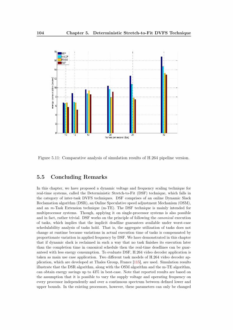
104 Chapter 5. Deterministic Stretch-to-Fit DVFS Technique
Figure 5.11: Comparative analysis of simulation results of H.264 pipeline version.
5.5 Concluding Remarks
In this chapter, we have proposed a dynamic voltage and frequency scaling technique forreal-time systems, called the Deterministic Stretch-to-Fit (DSF) technique, which falls inthe category of inter-task DVFS techniques. DSF comprises of an online Dynamic SlackReclamation algorithm (DSR), an Online Speculative speed adjustment Mechanism (OSM),and an m-Task Extension technique (m-TE). The DSF technique is mainly intended formultiprocessor systems. Though, applying it on single-processor systems is also possibleand in fact, rather trivial. DSF works on the principle of following the canonical executionof tasks, which implies that the implicit deadline guarantees available under worst-caseschedulability analysis of tasks hold. That is, the aggregate utilization of tasks does notchange at runtime because variations in actual execution time of tasks is compensated byproportionate variation in applied frequency by DSF. We have demonstrated in this chapterthat if dynamic slack is reclaimed in such a way that no task finishes its execution laterthan the completion time in canonical schedule then the real-time deadlines can be guar-anteed with less energy consumption. To evaluate DSF, H.264 video decoder application istaken as main use case application. Two different task models of H.264 video decoder ap-plication, which are developed at Thales Group, France [115], are used. Simulation resultsillustrate that the DSR algorithm, along with the OSM algorithm and the m-TE algorithm,can obtain energy savings up to 43% in best-case. Note that reported results are based onthe assumption that it is possible to vary the supply voltage and operating frequency onevery processor independently and over a continuous spectrum between defined lower andupper bounds. In the existing processors, however, these parameters can only be changed

5.5. Concluding Remarks 105
in predefined discrete steps. This assumption can be lifted in this case such that if thedesired optimal speed (corresponding to the achievable scalability of voltage/frequency) isnot available on a processor, it has to be approximated to the closest discrete level higherthan the optimal speed to prevent any deadline miss. Doing so could slightly marginalizedthe gains on energy. Through experiments, we illustrate that DSF is a competitive tech-nique for dynamic voltage and frequency scaling on a multiprocessor platform. Its runtimecomplexity is reduced, thanks to the online construction of canonical schedule, comparedto other techniques presented in [10] and [88]. The DSF technique is also integrated in ahybrid power and energy management scheme which is presented in chapter 6.
Currently, we are implementing DSF on a virtual platform for processor emulation,called QEMU [89], which is a generic and open source machine emulator and virtualizer.

Chapter 6
Hybrid Power ManagementScheme for Multiprocessor
Systems
Contents6.1 Introduction . . . . . . . . . . . . . . . . . . . . . . . . . . . . 1076.2 Related Work . . . . . . . . . . . . . . . . . . . . . . . . . . . . 1086.3 Hybrid Power Management Scheme . . . . . . . . . . . . . . 109
6.3.1 Machine-learning Algorithm . . . . . . . . . . . . . . . . . . . 1106.3.2 Selection of Experts . . . . . . . . . . . . . . . . . . . . . . . 114
6.4 Experiments . . . . . . . . . . . . . . . . . . . . . . . . . . . . 1146.4.1 Setup . . . . . . . . . . . . . . . . . . . . . . . . . . . . . . . 1146.4.2 Description of Experts . . . . . . . . . . . . . . . . . . . . . . 1156.4.3 Simulation Results . . . . . . . . . . . . . . . . . . . . . . . . 116
6.5 Concluding Remarks . . . . . . . . . . . . . . . . . . . . . . . 120
6.1 Introduction
As discussed in chapter 4 and 5, dynamic power management (DPM) and dynamic volt-age and frequency scaling (DVFS) policies are the most commonly used scheduling-basedpolicies for power and energy consumption management in modern embedded systems. Inthis chapter, we analyze some limitations of both these policies under different operatingconditions and discuss a mixed solution.
Dynamic Power management policies, as discussed in chapter 4, put system componentsinto power-efficient states whenever they are idle due to unavailability of workload. Onceapplied, DPM policies eliminate both dynamic as well as static power dissipation. How-ever, the inconvenience is that once in a power-efficient state, bringing a system componentback to the active/running state requires additional energy and/or latency to service anincoming task. Dynamic voltage and frequency scaling policies, on the other hand, exploitthe variations in actual workload of real-time tasks for dynamically adjusting voltage andfrequency to eventually reduce dynamic power dissipation. DVFS policies are known forreducing dynamic power dissipation quite aggressively, however, there are certain inconve-niences of DVFS policies due to physical limitations such as they cause increased leakageenergy drain by lengthening the interval over which a computation is carried out. Due tothe increasingly reduced feature-size, leakage power is becoming a significant contributing
108Chapter 6. Hybrid Power Management Scheme for Multiprocessor
Systems
factor in overall energy consumption. Moreover, the discrete number of voltage and fre-quency levels available in existing processor technology is a bottle-neck. Finding optimalreal-time voltage and frequency scaling on multiprocessors is NP-hard partition problemsince selectable processor frequency is discontinuous [46].
Both DPM and DVFS policies have their advantages and drawbacks. They both per-form well for specific set of operating conditions such as, for particular target applications,specific architecture configuration, and/or specific scheduling algorithms. However, bothpolicies often outperform each other when these operating conditions change [37]. For in-stance, a DVFS policy might perform well for applications that have large number of taskswith non-deterministic execution time of tasks (due to conditional branches) as compared toapplications that have small number of tasks or more deterministic execution time of tasks.Similarly, a DPM policy might perform well on processors, which have small recovery timeas compared to those who have large recovery time from power-efficient states for the sameapplication. Thus, no single policy, whether DPM or DVFS, fits perfectly in all or mostoperating conditions. This leads a designer to choose for an appropriate policy every timethere is a (desired or undesired) change in target application, architecture configuration, orscheduling algorithm. In this chapter, we have addressed the need of a common solutionwhich is adaptive to changing operating conditions. Based on the fact that most of thepower and energy management policies are designed for specific conditions, we propose anovel and generic scheme for energy and power management, called Hybrid Power Man-agement (HyPowMan) scheme. Instead of designing new power and energy managementpolicies to target specific operating conditions, this scheme takes a set of well-known exist-ing policies (DPM and/or DVFS), each of which performs well for a given set of conditions,and proposes a machine-learning mechanism to adapt at runtime to the best-performingpolicy for any given workload. The decision of applying suitable policy is taken online andadaptive to the varying workload. The HyPowMan scheme is generic in the sense that itpermits to integrate existing as well as new power and energy management policies andit can be applied under the control of global as well as partitioning-based scheduling al-gorithms. HyPowMan is intended mainly for multiprocessor real-time systems. However,applying it on single-processor systems is also possible. HyPowMan enhances the abilityof portable embedded systems to work with larger set of operating conditions by adaptingto the changing workloads and gives an overall performance that is better than any singlepolicy can offer.
6.2 Related Work
There exists an abundant literature about the DPM and the DVFS techniques that we havepreviously discussed in chapter 4 and chapter 5. In this chapter, we review the state-of-the-art on some recent research work related to the interplay of DPM and DVFS policies. Thegrowing importance of system-wide energy management clearly mandates the integrationof both DPM and DVFS policies. Yet, there are not many solutions available today whichuse both DVFS and DPM policies and capture their intriguing trade-off in a precise way.
Authors in [126] show that both DVFS and DPM solutions often work against eachother. That is, if the processing frequency is lowered through DVFS to save energy asillustrated in figure 6.1, the task execution time is extended (here, Cdvfs refers to elon-gated WCET of task due to slowdown). As a result, the idle time is shortened, whichprevents DPM from putting the devices into the power-efficient states (as the idle intervalmay become smaller than break-even time (BET)). On the other hand, the device energycan be reduced by executing the task at higher frequency to obtain enough idle time for
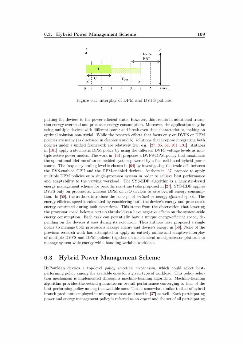
6.3. Hybrid Power Management Scheme 109
Figure 6.1: Interplay of DPM and DVFS policies.
putting the devices to the power-efficient state. However, this results in additional transi-tion energy overhead and processor energy consumption. Moreover, the application may beusing multiple devices with different power and break-even time characteristics, making anoptimal solution non-trivial. While the research efforts that focus only on DVFS or DPMpolicies are many (as discussed in chapter 4 and 5), solutions that propose integrating bothpolicies under a unified framework are relatively few, e.g., [27, 35, 64, 101, 131]. Authorsin [101] apply a stochastic DPM policy by using the different DVFS voltage levels as mul-tiple active power modes. The work in [131] proposes a DVFS-DPM policy that maximizesthe operational lifetime of an embedded system powered by a fuel cell based hybrid powersource. The frequency scaling level is chosen in [64] by investigating the trade-offs betweenthe DVS-enabled CPU and the DPM-enabled devices. Authors in [37] propose to applymultiple DPM policies on a single-processor system in order to achieve best performanceand adaptability to the varying workload. The SYS-EDF algorithm is a heuristic-basedenergy management scheme for periodic real-time tasks proposed in [27]. SYS-EDF appliesDVFS only on processors, whereas DPM on I/O devices to save overall energy consump-tion. In [58], the authors introduce the concept of critical or energy-efficient speed. Theenergy-efficient speed is calculated by considering both the device’s energy and processor’senergy consumed during task executions. This stems from the observation that loweringthe processor speed below a certain threshold can have negative effects on the system-wideenergy consumption. Each task can potentially have a unique energy-efficient speed, de-pending on the devices it uses during its execution. Thus authors have proposed a singlepolicy to manage both processor’s leakage energy and device’s energy in [58]. None of theprevious research work has attempted to apply an entirely online and adaptive interplayof multiple DVFS and DPM policies together on an identical multiprocessor platform tomanage system-wide energy while handling variable workload.
6.3 Hybrid Power Management Scheme
HyPowMan devises a top-level policy selection mechanism, which could select best-performing policy among the available ones for a given type of workload. This policy selec-tion mechanism is implemented through a machine-learning algorithm. Machine-learningalgorithm provides theoretical guarantee on overall performance converging to that of thebest-performing policy among the available ones. This is somewhat similar to that of hybridbranch predictors employed in microprocessors and used in [37] as well. Each participatingpower and energy management policy is referred as an expert and the set of all participating

110Chapter 6. Hybrid Power Management Scheme for Multiprocessor
Systems
policies collectively as expert set. Any multiprocessor DPM or DVFS policy that can guar-antee timing constraints for real-time systems is eligible to become member of expert set.When a processor is busy in executing tasks (also referred as active time), all DPM-basedexperts are inactive and are said to be dormant experts. However, DVFS-based expertscan (or cannot) be in inactive state depending on the workload. Conversely, whenever theprocessor is idle, all DVFS-based experts are dormant. Any expert, which is currentlyactive, is said to be working expert. A working expert solely governs all decisions relatedto power management on processors under the control of applied scheduling policy. Figure6.2 illustrates how different experts are arranged by the HyPowMan scheme in an SMParchitecture configuration under the control of global scheduling algorithm. For instance,expert3 in figure 6.2 is selected as working expert. Working expert returns to dormant state,which is the default state for all experts, once it finishes its job or another working expertreplaces it. The most critical task for HyPowMan is to select an appropriate expert for agiven power management opportunity. Power management opportunities such as idle timeintervals and dynamic slack time are also referred as input in the remaining of this chapter.Before the machine-learning algorithm is presented in detail, we emphasize a fundamentaldifference between DPM-based and DVFS-based experts. The power management oppor-tunities or input for DPM-based experts are the idle time intervals, which are inherentlypresent in an application’s schedule. Whereas, input for DVFS-based experts is dynamicslack, which is generated at runtime due to the variations in actual workload (to which,DPM-based experts can also exploit while chosen as working expert). Thus, challenges forthe HyPowMan scheme are: how to measure the performance (at runtime) for differentexperts that work for different kind of inputs, how to evaluate them, and how to employthem in a multiprocessor context. Note that the objective of HyPowMan is to convergetowards the best-performing policy within given expert set only and not to find the bestpossible energy savings under given operating conditions.
Figure 6.2: Arrangement of expert set under the HyPowMan scheme for an SMParchitecture.
6.3.1 Machine-learning Algorithm
Machine-learning algorithm employed in HyPowMan, which is an adaptation of Freund andSchapire’s online allocation algorithm presented in [43] and also used in [37], considers thatat most N (∀N , N ≥ 1) experts are present in expert set. The algorithm associates aweight vector W input with expert set, where W input= (winput1 , winput2 , ..., winputN ) consistsof weight factors corresponding to each expert k (∀k, 1 ≤ k ≤ N) for a given input. Every
6.3. Hybrid Power Management Scheme 111
time an input arrives, this weight vector is updated. Initially, weight factors of all individ-ual experts are equal and sum to one in order to provide equal opportunity for all expertsto perform well. However, these weights may not sum to one later during execution. Hy-PowMan maintains a probability vector Hinput associated with expert set, where Hinput=(hinput1 , hinput2 , ..., hinputN ) consists of probability factors corresponding to each expert k suchthat, (0 ≤ hinputk ≤ 1). This probability reflects the performance of an expert based on itsweight factor. It is obtained by normalizing weight factors as shown in equation 6.1. Theprobability factor provides a measure on each expert’s performance on previous input suchthat, at any point in time, the best-performing expert has the highest probability.
Hinput = W input/
N∑k=1
winputk (6.1)
HyPowMan selects expert with highest probability amongst all experts to become aworking expert on next input. In case the probability factors of multiple experts are equal,working expert is chosen randomly. Once selected, a working expert governs all decisionsrelated to power management under the control of scheduling policy. When an input isfinished, the performance of all experts is evaluated. Working expert is evaluated based onhow much energy was saved and how much performance degradation was incurred underthat particular expert. Dormant experts are evaluated based on how they would haveperformed if they had been selected as working expert. This evaluation is based on theloss factor of each expert. Loss factor is evaluated with respect to an ideal (offline) powermanagement policy that offers maximum possible energy savings and zero performancedegradation. The loss factor incurred by an expert k is referred as linputk . The value ofloss factor is a composition of loss in energy saving and performance degradation and it isinfluenced by their relative importance, which is expressed by factor α (∀α, 0 ≤ α ≤ 1).We refer to the loss factors corresponding to energy and performance as linputke and linputkp ,respectively, for expert k. Equation 6.2 represents joint loss factor of individual experts.
linputk = αlinputke + (1− α)linputkp (6.2)
Computation of loss factor slightly differs for DPM and DVFS experts. We elaboratethis difference in section 6.3.1.1. Once the joint loss factor linputk is calculated, final step inalgorithm is to update weight factors for each expert based on the loss they have incurredas shown by equation 6.3.
winput+1k = winputk βl
inputk (6.3)
Here, β is a constant such that (0 ≤ β ≤ 1). The value of β should be set between 0
and 1 depending on the granularity of weight factors, i.e. the higher the value of β is set,the lower the variation in weight occurs for a given input. Equation 6.3 depicts that theweight factors corresponding to experts with higher loss factors are reduced while for theexperts with lower loss factors are increased by simple multiplicative rule. This gives higherprobability of selecting better performing experts for the next input. Note that weight andprobability factors for all experts are updated once the input is terminated. Calculationsrelated to selecting the working expert (for next input) are performed during the activetime (i.e., the time when processors are executing tasks) and hence no additional overheador latency is incurred when the inputs actually occur. In other words, the time consumedin updating weight and probability factors should be masked with the execution time ofrunning tasks (for instance, in cases where dedicated hardware is used for schedulers) andtherefore, when a scheduling event arrives, a working expert is already selected. HyPowMan
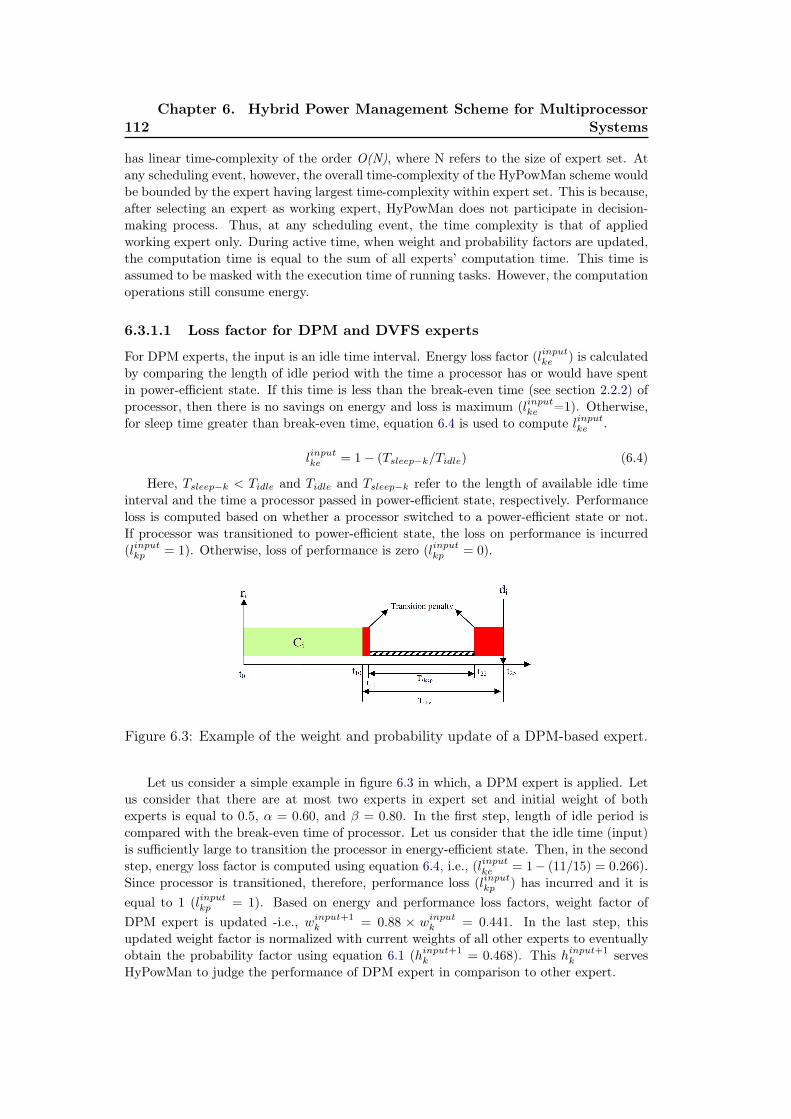
112Chapter 6. Hybrid Power Management Scheme for Multiprocessor
Systems
has linear time-complexity of the order O(N), where N refers to the size of expert set. Atany scheduling event, however, the overall time-complexity of the HyPowMan scheme wouldbe bounded by the expert having largest time-complexity within expert set. This is because,after selecting an expert as working expert, HyPowMan does not participate in decision-making process. Thus, at any scheduling event, the time complexity is that of appliedworking expert only. During active time, when weight and probability factors are updated,the computation time is equal to the sum of all experts’ computation time. This time isassumed to be masked with the execution time of running tasks. However, the computationoperations still consume energy.
6.3.1.1 Loss factor for DPM and DVFS experts
For DPM experts, the input is an idle time interval. Energy loss factor (linputke ) is calculatedby comparing the length of idle period with the time a processor has or would have spentin power-efficient state. If this time is less than the break-even time (see section 2.2.2) ofprocessor, then there is no savings on energy and loss is maximum (linputke =1). Otherwise,for sleep time greater than break-even time, equation 6.4 is used to compute linputke .
linputke = 1− (Tsleep−k/Tidle) (6.4)
Here, Tsleep−k < Tidle and Tidle and Tsleep−k refer to the length of available idle timeinterval and the time a processor passed in power-efficient state, respectively. Performanceloss is computed based on whether a processor switched to a power-efficient state or not.If processor was transitioned to power-efficient state, the loss on performance is incurred(linputkp = 1). Otherwise, loss of performance is zero (linputkp = 0).
Figure 6.3: Example of the weight and probability update of a DPM-based expert.
Let us consider a simple example in figure 6.3 in which, a DPM expert is applied. Letus consider that there are at most two experts in expert set and initial weight of bothexperts is equal to 0.5, α = 0.60, and β = 0.80. In the first step, length of idle period iscompared with the break-even time of processor. Let us consider that the idle time (input)is sufficiently large to transition the processor in energy-efficient state. Then, in the secondstep, energy loss factor is computed using equation 6.4, i.e., (linputke = 1− (11/15) = 0.266).Since processor is transitioned, therefore, performance loss (linputkp ) has incurred and it isequal to 1 (linputkp = 1). Based on energy and performance loss factors, weight factor ofDPM expert is updated -i.e., winput+1
k = 0.88 × winputk = 0.441. In the last step, thisupdated weight factor is normalized with current weights of all other experts to eventuallyobtain the probability factor using equation 6.1 (hinput+1
k = 0.468). This hinput+1k serves
HyPowMan to judge the performance of DPM expert in comparison to other expert.
6.3. Hybrid Power Management Scheme 113
For DVFS experts, the input is dynamic slack time. Similar to DPM experts, wheneverthere is an input available, the time it takes to scale Fop and Vdd is compared to availableslack time. If the amount of slack justifies the scaling of Fop and Vop to lower values andback to Fref and Vdd then the loss on energy is calculated using frequency scaling ratio.Otherwise, no gain on energy can be achieved by applying DVFS and thus, the loss ismaximum (linputke = 1). Performance loss is computed based on whether Fop and Vop werescaled or not. If scaling is applied, performance loss is incurred (linputkp = 1). Otherwise, noloss would have incurred (linputkp = 0).
Algorithm-9 presents our machine-learning algorithm. Suitable values for parameters(α and β corresponding to DPM and DVFS experts) should be specified by the user inaccordance with the relative importance of energy and performance loss factors for softreal-time applications (lines 1-4). Initial weights, as described earlier, are equal and sum toone in the beginning. Then the expert, which offers highest probability is selected to becomeworking expert at the start of next input (line 6). If all probability factors are equal, (whichis the case at start up) then any expert is chosen randomly to become working expert. Uponthe arrival of an input, the already selected working expert is applied (lines 7-8) and at theend of an input, each expert is evaluated and its weight and probability factors are updated(lines 9-11).
Algorithm 9 Machine-learning1: set parameters2:
{αdpm, αdvfs
}∈ [0, 1]
3:{βdpm, βdvfs
}∈ [0, 1]
4: w1k ∈ [0, 1] (∀k, 1 ≤ k ≤ N)
5: for all future inputs do6: select expert with maximum probability: hinput+1 = max
[hinputk
]7: if input arrives then8: apply selected expert as working expert9: else if input terminates then
10: update weight vector W input (apply equation 6.3)11: update probability vector H input (apply equation 6.1)
Note that HyPowMan has no direct control on the decision-making process of eitherexperts or scheduling algorithm itself. This scheme rather functions as a top-level entity,which evaluates the performance of different experts and based on previous performance,selects best-performing expert. Once selected, its the responsibility of an expert to providetemporal guarantees for real-time tasks as long as it is a working expert. Only those policiesproviding real-time guarantees are chosen to be member of expert set. Whenever a DVFS-based expert is switched by any other expert, all parameters of running/preempted tasksare reinstated with respect to nominal operating conditions (Vop, Fop). Similarly, when aDPM-based expert is switched by any other expert, all processors from power-efficient state(if any) are recovered until the newly selected working expert makes any decision abouttheir future state. Experts are switched, if necessary, only at scheduling events. Notethat once an expert is selected to be a working expert by HyPowMan, it has to wait forsuitable power management opportunities to appear in the application’s schedule beforemaking any decision according to its own rules. For instance, selection of a DPM expertas working expert does not imply that there are processors immediately put in power-
114Chapter 6. Hybrid Power Management Scheme for Multiprocessor
Systems
efficient state. Similarly, selection of a DVFS expert as working expert does not implythat processors’ speed is currently scaled. To take into account the latency in recoveringprocessors from energy-efficient states, processors are recovered before the newly selectedexpert starts decision-making.
6.3.2 Selection of Experts
The idea of HyPowMan is to propose an adaptive power and energy management schemefor relatively larger set of operating conditions. With the changes in workload characteris-tics and/or architecture configuration, it is possible that the designer/user is uncertain ofthe online behavior (strictly from energy consumption point of view) of a feasible targetapplication. In such case, it becomes tricky to choose an appropriate power-managementpolicy for changed operating conditions. In this section, we present some possible scenariosand discuss how HyPowMan can be used in each scenario.
Statically selected single expert: HyPowMan is able to apply a statically selectedsingle expert throughout runtime. This scenario is equivalent to applying any expert de-signed for specific operating conditions. However, offline decision of choosing specific expertis entirely dependent on user’s knowledge of application’s runtime behavior and target ar-chitecture. It is trivial to select an expert if designer has sufficient knowledge of operatingconditions and expert’s power- and energy-efficiency. There shall be no need to adapt onlineto other experts.
Statically selected profiling-based experts: In this scenario, when designer doesnot have sufficient knowledge of target application’s runtime behavior in order to determinea unique expert statically, profiling can be used to determine which experts would besuitable and in which order. In this scenario, the designer may statically apply each availableexpert and perform multiple iterations of simulation to determine how each expert performsduring various segments of simulation time. Based on these profiles, designer can determinewhich experts should be used and can also specify a priori order of selected experts fordifferent simulation segments -i.e., predefined instants at which, experts must be switched.Since statically selected single expert might not perform better throughout runtime of atarget application, therefore, profiling-based selection of experts permits a target applicationto exploit maximum energy gains under different experts as the time evolves.
Online selected experts: This is the scenario in which profiling does not help in deter-mining suitable expert(s) due to varying runtime behavior of target application. Machine-learning algorithm of HyPowMan is applied in this case to determine best-performing expertfor different simulation time segments online and experts are switched at runtime based onhow they perform. No predefined order of switching experts exists in this scenario.
6.4 Experiments
6.4.1 Setup
System model used for experiments in this chapter is the same as presented in chapter2 and used in chapters 4 and 5. EDF scheduling algorithm is used to schedule real-timeperiodic tasks. Energy consumption in processors is measured under the control of eachselected policy alone as well as under the control of HyPowMan. All results on energy
6.4. Experiments 115
consumption are scaled between 0.0 and 1.0 w.r.t. the worst-case energy consumption undernon-optimized algorithm within each simulation setting. That is, the energy consumed ina schedule of tasks under non-optimized algorithm, when all tasks execution with theirworst-case execution time, becomes reference (1.0) and all other values, including that ofnon-optimized algorithm, are scaled. Moreover, it is demonstrated how the variations in αand β alter the convergence of HyPowMan towards best-performing expert. All simulationsare performed for online selected experts scenario as mentioned in section 6.3.2.
6.4.2 Description of Experts
In this section, different experts that are used for experiments are described. There arethree power/energy management policies (one DPM and two DVFS policies) being selectedfor experiments. These policies are: Timeout DPM policy, DSF (DVFS) policy, and ccEDF(DVFS) policy. In the following, we provide a brief description of these policies.
Timeout DPM policy: Timeout DPM policy is presented in [61]. In this policy,whenever there is no task to service, processor waits for a specified amount of time beforetransitioning to energy-efficient state. Value of timeout can be fixed or it may be changedover time statically. Timeout DPM policy is one of the most widely used policies in manyapplications because of its simplicity.
DSF (DVFS) policy: Deterministic Stretch-to-Fit (DSF) DVFS policy is presentedin detail in chapter 5 and also in [19]. This policy is based on an online slack reclamationalgorithm, which permits the dynamic slack, produced by the precedent task, to be fullyconsumed by single subsequent task at the appropriate priority level. Such greedy allocationof slack allows large variations in Fop and Vop, which eventually results in larger gains onenergy consumption.
ccEDF (DVFS) policy: Cycle-conserving Earliest Deadline First (ccEDF) DVFS pol-icy is presented in [87]. In this policy, the dynamic slack time is redistributed globally to allready tasks. ccEDF considers actual execution time of all terminated tasks until their nextrelease and worst-case execution time of all ready and running tasks to determine concur-rent resource utilization of application and calculate required scaling factor for speed. Oncescaling factor is determined, frequency and voltage are scaled globally on all processors.
6.4.2.1 Target application
Synthetic task sets are considered in these experiments in order to estimate energy con-sumption as a function of variations in three parameters –i.e., variations in total utilizationUsum(τ), number of tasks (n), and best-case to worst-case execution time ratio (bcet/wcet)of each task. For each data point, a task set is randomly generated, in which, each task hasa uniform probability to have small (5− 25ms), medium (25− 75ms), or long (75− 120ms)periods. All task periods are uniformly distributed among these three ranges. Note that asimilar period generation scheme is used in [1, 87]. Individual utilization of each task ui isalso generated randomly.
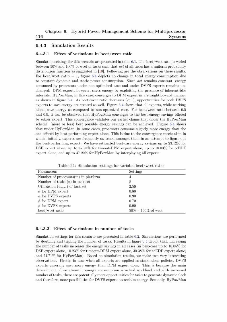
116Chapter 6. Hybrid Power Management Scheme for Multiprocessor
Systems
6.4.3 Simulation Results
6.4.3.1 Effect of variations in bcet/wcet ratio
Simulation settings for this scenario are presented in table 6.1. The bcet/wcet ratio is variedbetween 50% and 100% of wcet of tasks such that aet of all tasks has a uniform probabilitydistribution function as suggested in [10]. Following are the observations on these results.For bcet/wcet ratio = 1, figure 6.4 depicts no change in total energy consumption dueto constant dynamic and static power consumption. Since aet remains constant, energyconsumed by processors under non-optimized case and under DVFS experts remains un-changed. DPM expert, however, saves energy by exploiting the presence of inherent idleintervals. HyPowMan, in this case, converges to DPM expert in a straightforward manneras shown in figure 6.4. As bcet/wcet ratio decreases (< 1), opportunities for both DVFSexperts to save energy are created as well. Figure 6.4 shows that all experts, while workingalone, save energy as compared to non-optimized case. For bcet/wcet ratio between 0.5
and 0.9, it can be observed that HyPowMan converges to the best energy savings offeredby either expert. This convergence validates our earlier claims that under the HyPowManscheme, (more or less) best possible energy savings can be achieved. Figure 6.4 showsthat under HyPowMan, in some cases, processors consume slightly more energy than theone offered by best-performing expert alone. This is due to the convergence mechanism inwhich, initially, experts are frequently switched amongst them in an attempt to figure outthe best-performing expert. We have estimated best-case energy savings up to 23.12% forDSF expert alone, up to 47.94% for timout-DPM expert alone, up to 18.03% for ccEDFexpert alone, and up to 47.22% for HyPowMan by interplaying all experts.
Table 6.1: Simulation settings for variable bcet/wcet ratioParameters SettingsNumber of processors(m) in platform 4Number of tasks (n) in task set 8Utilization (usum) of task set 2.50α for DPM expert 0.80α for DVFS experts 0.90β for DPM expert 0.70β for DVFS experts 0.90bcet/wcet ratio 50%− 100% of wcet
6.4.3.2 Effect of variations in number of tasks
Simulation settings for this scenario are presented in table 6.2. Simulations are performedby doubling and tripling the number of tasks. Results in figure 6.5 depict that, increasingthe number of tasks increases the energy savings in all cases (in best-case up to 18.05% forDSF expert alone, 10.23% for timeout-DPM expert alone, 30.38% for ccEDF expert alone,and 24.71% for HyPowMan). Based on simulation results, we make two very interestingobservations. Firstly, in case when all experts are applied as stand-alone policies, DVFSexperts generally save more energy than DPM expert does. This is because the maindeterminant of variations in energy consumption is actual workload and with increasednumber of tasks, there are potentially more opportunities for tasks to generate dynamic slackand therefore, more possibilities for DVFS experts to reclaim energy. Secondly, HyPowMan

6.4. Experiments 117
Figure 6.4: Simulation results on variation of bcet/wcet ratio.
can even result in energy savings more than any stand-alone policy in some cases. Thisis because, over entire simulation time, a single expert cannot always change a processor’spower consumption profile (often due to transition costs). HyPowMan, on the other hand,switches an expert with the other if it is not performing well under such conditions andeventually results is better energy savings.
Table 6.2: Simulation settings for variable number of tasksParameters SettingsNumber of processors(m) in platform 4Number of tasks (n) in task set 8, 16, & 24Utilization (usum) of task set 2.50α for DPM expert 0.80α for DVFS experts 0.90β for DPM expert 0.70β for DVFS experts 0.90bcet/wcet ratio 60% of wcet
6.4.3.3 Effect of variations in aggregate utilization
Simulation settings for this scenario are presented in table 6.3. Multiple task sets withtotal utilization varying between 50% (lower workload) and 100% (maximum workload) ofplatform capacity have been generated. Results in figure 6.6 depict that the difference inenergy savings for a given utilization is more or less the same in all cases. That is, thevariations in aggregate utilization do not significantly vary the performance of these poli-cies and lesser workload naturally favors more energy savings on fixed capacity platforms.
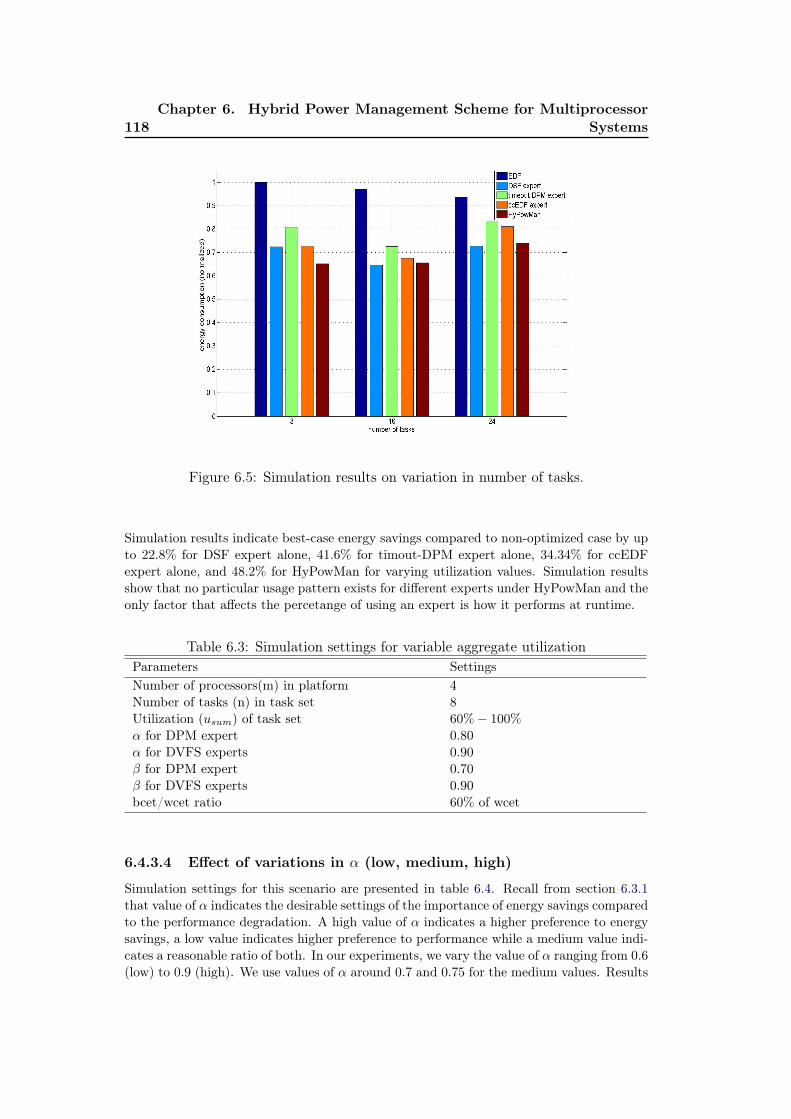
118Chapter 6. Hybrid Power Management Scheme for Multiprocessor
Systems
Figure 6.5: Simulation results on variation in number of tasks.
Simulation results indicate best-case energy savings compared to non-optimized case by upto 22.8% for DSF expert alone, 41.6% for timout-DPM expert alone, 34.34% for ccEDFexpert alone, and 48.2% for HyPowMan for varying utilization values. Simulation resultsshow that no particular usage pattern exists for different experts under HyPowMan and theonly factor that affects the percetange of using an expert is how it performs at runtime.
Table 6.3: Simulation settings for variable aggregate utilizationParameters SettingsNumber of processors(m) in platform 4Number of tasks (n) in task set 8Utilization (usum) of task set 60%− 100%
α for DPM expert 0.80α for DVFS experts 0.90β for DPM expert 0.70β for DVFS experts 0.90bcet/wcet ratio 60% of wcet
6.4.3.4 Effect of variations in α (low, medium, high)
Simulation settings for this scenario are presented in table 6.4. Recall from section 6.3.1that value of α indicates the desirable settings of the importance of energy savings comparedto the performance degradation. A high value of α indicates a higher preference to energysavings, a low value indicates higher preference to performance while a medium value indi-cates a reasonable ratio of both. In our experiments, we vary the value of α ranging from 0.6(low) to 0.9 (high). We use values of α around 0.7 and 0.75 for the medium values. Results
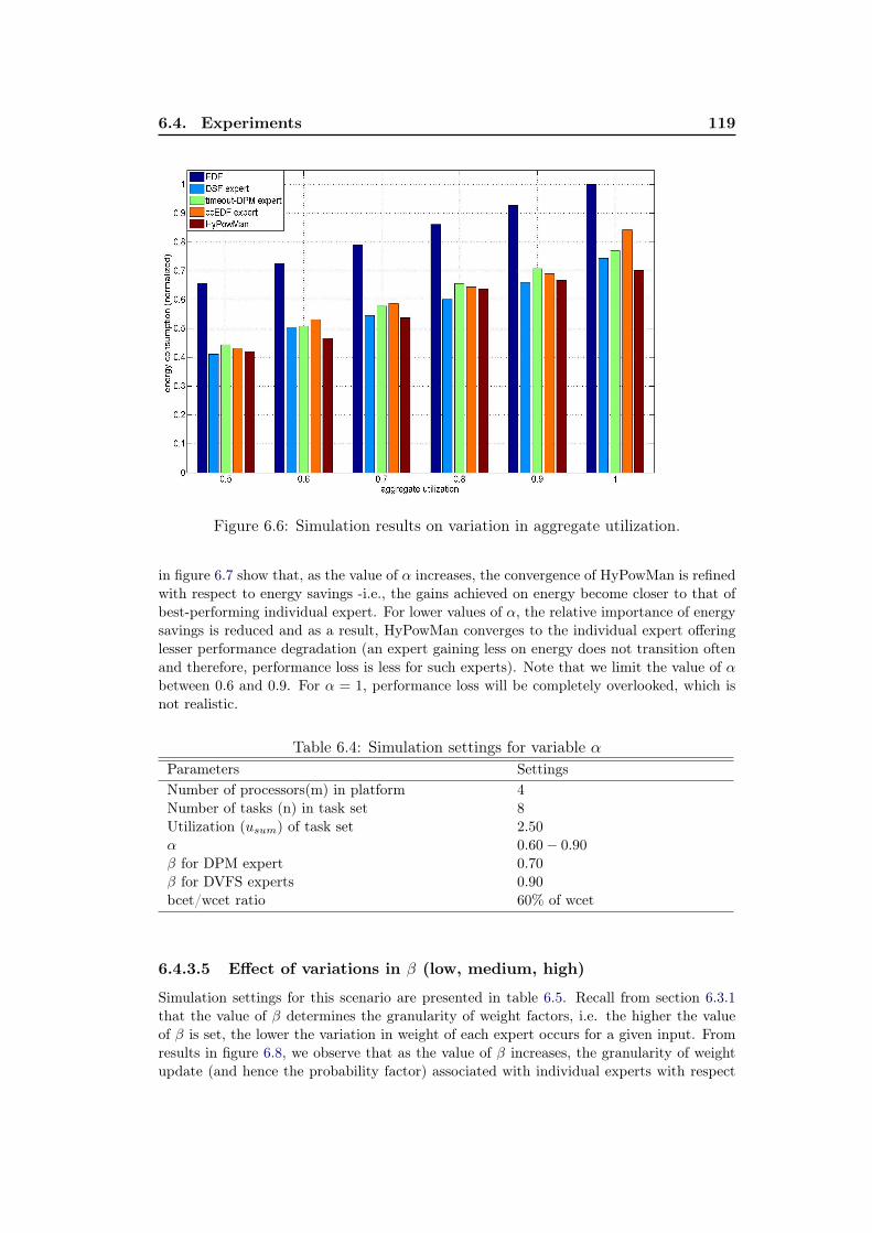
6.4. Experiments 119
Figure 6.6: Simulation results on variation in aggregate utilization.
in figure 6.7 show that, as the value of α increases, the convergence of HyPowMan is refinedwith respect to energy savings -i.e., the gains achieved on energy become closer to that ofbest-performing individual expert. For lower values of α, the relative importance of energysavings is reduced and as a result, HyPowMan converges to the individual expert offeringlesser performance degradation (an expert gaining less on energy does not transition oftenand therefore, performance loss is less for such experts). Note that we limit the value of αbetween 0.6 and 0.9. For α = 1, performance loss will be completely overlooked, which isnot realistic.
Table 6.4: Simulation settings for variable αParameters SettingsNumber of processors(m) in platform 4Number of tasks (n) in task set 8Utilization (usum) of task set 2.50
α 0.60− 0.90
β for DPM expert 0.70β for DVFS experts 0.90bcet/wcet ratio 60% of wcet
6.4.3.5 Effect of variations in β (low, medium, high)
Simulation settings for this scenario are presented in table 6.5. Recall from section 6.3.1that the value of β determines the granularity of weight factors, i.e. the higher the valueof β is set, the lower the variation in weight of each expert occurs for a given input. Fromresults in figure 6.8, we observe that as the value of β increases, the granularity of weightupdate (and hence the probability factor) associated with individual experts with respect

120Chapter 6. Hybrid Power Management Scheme for Multiprocessor
Systems
Figure 6.7: Simulation results on variation in α.
Table 6.5: Simulation settings for variable βParameters SettingsNumber of processors(m) in platform 4Number of tasks (n) in task set 8Utilization (usum) of task set 2.50
α for DPM expert 0.80α for DVFS experts 0.90β 0.60− 0.90
bcet/wcet ratio 60% of wcet
to their performance is refined. This refinement in weight update permits HyPowMan tomore precisely evaluate the performance of working expert as well as dormant experts, whicheventually leads to a better convergence to best-performing expert. However, increasing βtoo much can result in increasing the sensitivity of HyPowMan towards weight updatesand can cause increased switching of experts. Moreover, when the value of β is decreasedtoo much, HyPowMan has lesser precision in weight updates and therefore, frequentlyswitches the working expert again, which eventually leads to lesser gains on energy andmore performance loss.
6.5 Concluding Remarks
In this chapter, we have proposed a generic power and energy management scheme formultiprocessor systems, called Hybrid Power Management (HyPowMan) scheme. HyPow-Man serves as a top-level entity which, instead of designing new power management policies(whether DPM or DVFS) for specific operating conditions, takes a set of well-known existingpolicies, each of which performs well for a given set of conditions, and adapts at runtime to

6.5. Concluding Remarks 121
Figure 6.8: Simulation results on variation in β.
the best-performing policy for any given workload. A machine-learning algorithm is imple-mented to evaluate the performance of all policies and the decision to select best-performingpolicy at any point in time is taken online and adaptive to the varying workload. Experi-ments validate that our proposed scheme adapts well to the changing workload and quicklyconverges to the best-performing policy within the selected expert set by a margin of 1.5%
to 11% (w.r.t. best-case) on energy savings. Through experiments, we have validated thatHyPowMan is robust to variations in application task parameters such as actual executiontime, number of tasks, and aggregate utilization. The expert set used for experiments inthis chapter is composed of both DPM and DVFS policies. However, we have also validatedthe working of HyPowMan by using similar policies only –i.e., only DVFS or only DPMpolicies. Moreover, experiments using AsDPM policy (chapter 4), along with DSF policy(chapter 5), were also performed. Interested reader can find those results in Appendix B.One of the limitations of HyPowMan is that it evaluates the performance of all experts(working as well as dormant) for every input (i.e. power- and energy-saving opportunity),which may increase the computational overhead if larger expert sets are used. This aspectrequires improvements for an efficient implementation on hardware platforms.


Chapter 7
Conclusions and Future ResearchPerspectives
Real-time embedded systems have become ubiquitous in our life, ranging from hand-heldcell phones and home appliances to more sophisticated systems like data centers, signal-processing systems, satellites, and military applications. As the uses for real-time systemsbecome diverse, the research on these systems has confronted with many emerging chal-lenges. Nowadays, real-time applications have become sophisticated and complex in theirbehavior and interaction. Their sophistication and complexity has led to the emergence ofmultiprocessor architectures. Another reason for multiprocessor architectures to be read-ily acceptable in commercial sector is that they have been considered as a solution to thethermal roadblock imposed by single-processor architectures. It has become clearer thatin future, most of the sophisticated real-time applications will be deployed on multipro-cessor platforms. Inevitably, the change in platform architecture design and complexityof real-time applications have renewed some existing challenges as well as brought somenew ones for real-time research community. One of the major renewed challenge is thatsingle-processor optimal scheduling algorithms can not be applied on multiprocessor sys-tems without loss of optimality. Thus, the real-time research community has to developalternative scheduling strategies to incorporate the aspects of multiprocessor systems. Oneof the new challenges that real-time systems are facing is to reduce power and energyconsumption while maintaining assurance that timing constraints will be met. As the com-putational demands of real-time embedded systems continue to grow, effective yet trans-parent energy-management approaches are becoming increasingly important to minimizeenergy consumption, extend battery life, and reduce thermal effects. Power and energyconsumption in real-time systems has earned great importance over the last few years andmany software-based approaches to statically as well as dynamically reduce power andenergy consumption have been proposed. Software-based solutions, particularly energy-aware scheduling techniques such as dynamic voltage & frequency scaling and dynamicpower management techniques have emerged. Furthermore, system-wide energy-efficienttechniques that include other system components such as memory sub-systems and inter-connect network have been proposed as well. Yet their flexibility is often matched by thecomplexity of the solution.
This dissertation is an attempt to ameliorate energy-management in real-time embed-ded systems by proposing new flexible and effective energy-aware scheduling strategies.Techniques proposed in this dissertation increase the set of operating conditions in which,real-time applications can be scheduled in an energy-efficient manner while maintainingtheir temporal guarantees on multiprocessor platforms. We divide this chapter into twoparts. First part summarizes our contributions and the significance of results obtained.The second part presents some future research perspectives and ameliorations related tothis dissertation.
124 Chapter 7. Conclusions and Future Research Perspectives
7.1 Summary of Contributions and Results
In this section, we summarize the contributions of this dissertation.
Two-Level Hierarchical Scheduling Algorithm. Restricted-migration schedul-ing strategies provide a good compromise between the full migration and the partitioningstrategies [24, 63, 62]. It is flexible enough to allow dynamic tasks to join the system atruntime, but it does not incur large migration overheads as compared to full-migrationstrategies. In this dissertation, in chapter 3, we have presented a multiprocessor schedul-ing algorithm, called two-level hierarchical scheduling algorithm (2L-HiSA), which falls inthe category of restricted migration scheduling. The EDF scheduling algorithm has theleast runtime complexity among job-level fixed-priority algorithms for scheduling tasks onmultiprocessor architecture. However, EDF suffers from sub-optimality in multiprocessorsystems. 2L-HiSA addresses the sub-optimality of EDF as global scheduling algorithm anddivides the problem into a two-level hierarchy of schedulers. 2L-HiSA uses multiple in-stances of single-processor optimal EDF scheduling algorithm in a hierarchical fashion attwo levels: an instance of EDF at top-level scheduler and an instance at local-level scheduleron every processor of the platform.
Moreover, 2L-HiSA consists of two phases: 1) the task-partitioning phase, in which, eachnon-migrating task is assigned to a specific processor by following the bin-packing approach,2) the processor-grouping phase, in which, processors are grouped together based on theirworkload characteristics. 2L-HiSA partitions application tasks statically onto processorsby following the bin-packing approach, as long as schedulability of tasks partitioned on aparticular processor is not violated. Tasks that can not be partitioned on any processor inthe platform qualify as migrating or global tasks. Furthermore, it makes clusters of identicalprocessors such that, per cluster, the unused fragmented computation power equivalent toat most one processor is available. We show that 2L-HiSA improves on the schedulabilitybound of restricted-migration based scheduling using multiple instances of preemptive EDFfor multiprocessor systems. 2L-HiSA can ensure deadline guarantees if a subset of tasks canbe partitioned such that the under-utilization per cluster of processors remain less than orequal to the equivalent of one processor. Partitioning tasks on processors reduces schedulingrelated overheads such as context switch, preemptions, and migrations, which eventuallyhelp reducing overall energy consumption. The NP-hardness of partitioning problem [60],however, can often be a limiting factor. By using clusters of processors instead of consideringindividual processors, 2L-HiSA alleviates bin-packing limitations by effectively increasingbin sizes in comparison to item sizes. With a cluster of processors, it is much easier toobtain the unused processing power per cluster less than or equal to one processor. Weprovide simulation results to support our proposition. We have illustrated that power- andenergy-efficient strategies like DVFS and/or DPM can be used in conjunction with 2L-HiSAto improve energy savings. Furthermore, we have illustrated that the task preemption- andmigration-related overhead is significantly less when using 2L-HiSA as compared to PFairand ASEDZL, which are multiprocessor optimal scheduling algorithms.
Assertive Dynamic Power Management Technique. Another contribution ofthis dissertation, presented in chapter 4, is the proposition of a dynamic power managementtechnique for multiprocessor real-time systems. DPM techniques achieve energy conserva-tion in embedded computing systems by actively changing the power consumption profileof the system by selectively putting its components into power-efficient states sufficient tomeeting functionality requirements. Our proposed technique is called Assertive Dynamic
7.1. Summary of Contributions and Results 125
Power Management (AsDPM) technique because of its aggressiveness towards the extrac-tion of the idle time intervals, if present, from the application’s runtime schedule which isnot the case in conventional DPM techniques. AsDPM technique works under the controlof global EDF and global LLF scheduling algorithms. It is an admission control techniquefor real-time tasks which makes a feasible task set energy efficient by deciding when exactlya ready task shall execute. Without this admission control, all ready tasks are executed assoon as there are enough computing resources (processors) available in the system, leadingto poor possibilities of putting some processors into power-efficient states. AsDPM tech-nique differs from the existing DPM techniques in the way it exploits the idle time intervals.A conventional DPM technique can exploit idle intervals only once they occur on a processor–i.e., once an idle interval is detected. Upon detecting idle time intervals, these techniquesdecide whether to transition target processor(s) to power-efficient state. AsDPM technique,on the other hand, aggressively extracts all idle intervals from some processors and clustersthem on some other processors of the platform to elongate the duration of idle time. Tran-sitioning processors to suitable power-efficient state then become a matter of comparingidle interval’s length against the break-even time (BET) of target processor. Although,AsDPM is an online dynamic power management technique, its working principle can beused to determine static optimal architecture configurations (i.e., number of processors andtheir corresponding voltage-frequency level, which is required to meet real-time constraintsin worst-case with minimum energy consumption) for target application through simula-tions. In this dissertation, we have demonstrated the use of AsDPM for determining staticoptimal architecture configurations at first, and then as an online DPM technique, whichcan further increase energy-efficiency of already (statically) optimized configurations.
Deterministic Stretch-to-Fit DVFS Technique. Dynamic voltage and frequencyscaling is one of the effective techniques, which aim at changing energy consumption pro-file of real-time embedded systems. This is because energy consumption of processors is aquadratic function of supply voltage of processors [48]. Real-time applications potentiallyexhibit variations in their actual execution time and therefore, often finish much earlier thantheir estimated worst-case execution time. Real-time DVFS techniques exploit these varia-tions in actual workload for dynamically adjusting the voltage and frequency of processorsin order to reduce power consumption. In this dissertation, in chapter 5, we propose aninter-task dynamic voltage and frequency scaling technique for real-time multiprocessor sys-tems, called Deterministic Stretch-to-Fit (DSF) technique. The DSF technique comprisesthree algorithms, namely, Dynamic Slack Reclamation (DSR) algorithm, Online Specula-tive speed adjustment Mechanism (OSM), and m-Tasks Extension (m-TE) algorithm. TheDSR algorithm is the principle slack reclamation algorithm of DSF that assigns dynamicslack, produced by a precedent task, to the appropriate priority next ready task that wouldexecute on the same processor. While using DSR, dynamic slack is not shared with otherprocessors in the system. Rather, slack is fully consumed on the same processor by thetask, to which it is once attributed. Such greedy allocation of slack allows the DSR al-gorithm to have large slowdown factor for scaling voltage and frequency for a single task,which eventually results in improved energy savings. DSR works in conjunction with globalscheduling algorithms on identical multiprocessor real-time systems. The OSM and them-TE algorithms are extensions of the DSR algorithm. The OSM algorithm is an online,adaptive, and speculative speed adjustment mechanism, which anticipates early completionof tasks and performs aggressive slowdown on processor speed. Apart from saving moreenergy as compared to the stand-alone DSR algorithm, this speculative speed adjustmentmechanism also helps to avoid radical changes in operating frequency and supply voltage,

126 Chapter 7. Conclusions and Future Research Perspectives
which results in reduced peak power consumption, which leads to an increase in battery lifefor portable embedded systems. The m-TE algorithm extends an already existing One-TaskExtension (OTE) technique for single-processor systems onto multiprocessor systems.
DSF works on the principle of following the canonical execution of tasks, which impliesthat the implicit deadline guarantees available under worst-case schedulability analysis oftasks hold. That is, the aggregate utilization of tasks does not change at runtime becausevariations in actual execution time of tasks is compensated by proportionate variation inapplied frequency by DSF. We have demonstrated in this chapter that if dynamic slackis reclaimed in such a way that no task finishes its execution later than the completiontime in canonical schedule then the real-time deadlines can be guaranteed with less energyconsumption. To evaluate DSF, H.264 video decoder application is taken as main usecase application. Two different task models of H.264 video decoder application, which aredeveloped at Thales Group, France [115], are used. Simulation results illustrate that theDSR algorithm, along with the OSM algorithm and the m-TE algorithm, can obtain energysavings up to 43% in best-case. Note that reported results are based on the assumptionthat it is possible to vary the supply voltage and operating frequency on every processorindependently and over a continuous spectrum between defined lower and upper bounds.In section 7.2, we discuss how removing this assumption can effect the working of DSF.
Hybrid Power Management Technique. Both dynamic power management(DPM) and dynamic voltage & frequency scaling (DVFS) policies are the most commonlyused scheduling-based policies for power/energy consumption management in modernembedded systems. They both perform well for specific set of operating conditions suchas, for particular target applications, specific architecture configuration, and/or specificscheduling algorithms. However, both policies often outperform each other when theseoperating conditions change. Thus, no single policy, whether DPM or DVFS, fits perfectlyin all or most operating conditions, leading a designer to choose for an appropriate policyevery time there is a change in target application, architecture configuration, or schedulingalgorithm. In this dissertation, in chapter 6, we have addressed the need of a commonsolution which is adaptive to changing operating conditions. Based on the fact thatmost of the power/energy management policies are designed for specific conditions, wepropose a generic power/energy management scheme called Hybrid Power Management(HyPowMan) scheme. Instead of designing new power/energy management policies (DPMor DVFS) to target specific operating conditions, HyPowMan scheme takes a set ofwell-known existing policies, each of which performs well for a given set of conditions,and proposes a machine-learning mechanism to adapt at runtime to the best-performingpolicy for any given workload. The decision of applying suitable policy is taken onlineand adaptive to the varying workload. HyPowMan scheme is generic in the sense that itpermits to integrate existing as well as new power/energy management policies and it canbe applied under the control of global as well as partitioning-based scheduling algorithms.This scheme serves as a top-level entity of all power management policies within anexpert-set. It does not intervene in decision-making process of either controlling schedulingalgorithm or applied (working) expert. The job of HyPowMan scheme is only to select abest-performing expert from expert-set based on its performance. Once selected, an expertmakes all power management decisions under the control of scheduling algorithm. Thus,HyPowMan scheme enhances the ability of embedded real-time systems to adapt withchanging workload by working with a larger set of operating conditions and gives overallperformance and energy savings that are better than any single policy can offer. Utilityof HyPowMan scheme can be extended beyond energy-efficiency –i.e., the adaptivity of
7.2. Future Research Perspectives 127
HyPowMan scheme allows to define other performance parameters as principle criteria forconverging to the best-performing expert. For instance, peak power consumption, batterylife, and temperature threshold can be the principle criteria for HyPowMan scheme foradapting to the best-performing expert.
7.2 Future Research Perspectives
Real-time systems have very complex characteristics. Changing one aspect of the systemcan result in a very different problem. In this dissertation, we have focused mainly onachieving the energy-efficiency in real-time multiprocessor systems through scheduling. Ourcontributions deal with specific models of tasks and processing platform which are discussedin chapter 2. Generalization of these models expands the number of possible systems thatcan be used by the real-time applications. Therefore, further extensions of this work includegeneralizing the task model and processing model. Many of these generalized models willrequire certain ameliorations in our proposed techniques that we discuss in this section.
7.2.1 Task Models
Inter-Task Dependency. The research work presented in this dissertation assumesan independent and preemptive task model –i.e., the execution of one task’s job is notcontingent upon the status of another task’s job. There are many problems in which in-dependence is an unreasonable assumption. Also, in some cases preemption may not beallowed. Jobs may have dependencies for a variety of reasons. Two types of job dependen-cies are resource sharing and precedence constraints. Incorporating resource sharing andprecedence constraints into the results presented in this dissertation would be a naturalextension. However, dependencies between tasks can cause priority inversions –situationswhere a higher priority job is blocked while a lower priority job executes. Such priorityinversions may violate our assumptions. For instance, in case of 2L-HiSA scheduling algo-rithm, two tasks with precedence constraint may require to be statically assigned on thesame processor, thus adding another limitation along with the partitioning problem. Sim-ilarly, in case of AsDPM technique, resource sharing between tasks may cause a processorto stand still in idle state that could have been otherwise, transitioned to power-efficientstate as soon as the runtime workload is reduced.
Task Preemption. Task preemption is a common assumption in real-time systems,however, there are situations when jobs may not be preempted. Removing the ability topreempt jobs may cause priority inversions. Moreover, non-preemptive systems can alsosuffer from scheduling anomalies whereby a feasible system may miss deadlines if one ormore jobs are removed from the system or complete executing early. Accounting for priorityinversions and scheduling anomalies can be an important extension to the research presentedin this dissertation. However, we did not consider non-preemptive systems. Moreover, wehave considered only feasible task systems with no scheduling anomalies.
Period of Task. Another common assumption in real-time systems is about the taskmodels based on their periodicity. This parameter can be interpreted in three distinct ways,each of which leads to a well-defined type of task. According to the interpretation given tothe period, tasks can be classified into three categories: periodic task model, sporadic taskmodel, and aperiodic task model. In this dissertation, we have considered periodic task
128 Chapter 7. Conclusions and Future Research Perspectives
models –i.e., every task has an exact inter-arrival time between successive jobs. Extendingour proposed techniques to sporadic and aperiodic task models would be an interestingcontribution as it would allow the handling of a wide range of real-time applications.
7.2.2 Platform Architectures
This dissertation considers homogeneous multiprocessor platform of type SMP (Symmet-ric shared-memory Multiprocessor) composed of identical processors. There are a varietyof ways in which the processing platform model can be generalized. For instance, uni-form multiprocessor or unrelated multiprocessor platforms can be used instead of identicalmultiprocessor platform. Certain contributions of this dissertation, such as AsDPM andDSF techniques, have been used in French national project Pherma [86]. This projectproposes a heterogeneous CMP (Chip Multi-Processing) processing platform model calledSCMP (Scalable Chip Multi-Processing) that supports dynamic migration and preemptionof tasks by using physically distributed, logically shared memories [120]. The heterogene-ity in SCMP platform is inter-cluster of processing units (i.e., multiple clusters/groupsof identical processors are formed, however, different clusters can contain different typeof processing units). SCMP is good alternative platform compared to SMP platform forfurther extensions of our proposed techniques. Furthermore, the results presented in thisdissertation consider mostly the power and energy consumption of processors only and didnot include energy consumed by other sub-systems such as memory and interconnect net-work. Recent research reports that peripheral devices, memory subsystems, flash drives,and wireless network interfaces are pervasive in modern embedded systems that consumeconsiderable amount of energy. In order to achieve system-wide energy savings, energy-aware I/O scheduling algorithms need to be developed for real-time systems. Extension ofour proposed techniques to system-wide energy-efficient techniques is a possible direction.For instance, we have demonstrated in chapter 4 that AsDPM technique can be useful formemory subsystems. HyPowMan scheme can also incorporate the energy consumption ofperipheral devices and other subsystems while selecting suitable experts.
Another aspect concerning the generalization of processing platform is the method ofscaling voltage & frequency in processors that support multiple voltage-frequency levels.In this dissertation, we have considered that it is possible to vary the voltage & frequencyon every processor independently and over a continuous spectrum between defined lowerand upper bounds. This consideration is based on the fact that processors that are able tooperate on a (more or less) continuous voltage and frequency spectrum are fast becominga reality [10]. However, this assumption can be lifted for processors offering only discretevoltage-frequency levels such that if the (calculated) optimal processor speed is not availableon a processor, it has to be approximated to the closest discrete level higher than theoptimal speed to prevent any deadline miss. This conversion is straightforward for tasksthat satisfy sufficient schedulability bound. For a feasible task set satisfying only necessaryschedulability condition, converting to discrete operating frequency would mean variationin concurrent utilization at runtime, which could lead to deadline misses. This aspect wouldrequire slight ameliorations for DSF technique for instance, which is based on the principleof following canonical execution of tasks.
7.2.3 Scheduling Algorithms
Most of the contributions presented in this dissertation consider the earliest deadline first(EDF) scheduling algorithm for scheduling real-time tasks on a multiprocessor platform.Even though there are many reasons why EDF is a reasonable scheduling algorithm to
7.2. Future Research Perspectives 129
consider, it is pertinent to ask whether the contributions presented in this dissertationcan work in conjunction with other scheduling algorithms as well. We have discussed inchapter 3 that EDF algorithm has the least runtime complexity for scheduling tasks onmultiprocessor architectures, but it suffers from sub-optimality in multiprocessor context.To improve the schedulability bound of EDF-based systems, we have proposed 2L-HiSAalgorithm which uses multiple instances of single-processor optimal EDF algorithm in ahierarchy of schedulers. For the remaining contributions of this dissertation, extendingthem while using other algorithms would be a valuable future contribution. We discussthe possibilities of extending our proposed techniques to other multiprocessor schedulingalgorithms in the following.
AsDPM Technique. Extending AsDPM technique to any of the multiprocessorscheduling algorithm which is based on the fluid scheduling mechanism (for instance, PFair[13] and LLREF [28] algorithms) is not possible due to their contradiction with the work-ing principle of AsDPM technique. In algorithms based on fluid scheduling mechanism,all ready tasks should execute proportionately to their respective utilization (or so calledweight). In AsDPM technique, on the other hand, a ready task can be deferred (delayed)from execution until and unless its anticipative laxity becomes negative (see chapter 4),which is contrary to the working principles of LLREF, PFair, and its heuristic algorithms.It is possible, however, to extend AsDPM technique to other algorithms such as LLF [71].
DSF Technique. It is possible to extend all three algorithms –i.e., DSR, OSM, and m-TE, presented under DSF technique to other scheduling algorithms. Since DSF techniqueworks on the principle of following canonical execution of tasks, therefore, it is possibleto integrate DSF technique with other algorithms with slight changes in the method ofcalculating and attributing dynamic slack at runtime.
HyPowMan Scheme. HyPowMan scheme itself does not intervene in the decision-making process of either scheduling algorithm or selected working expert (power-management strategy). Thus, it is possible to implement HyPowMan scheme with otherscheduling algorithms. The only limiting factor can be the overall time complexity of thesystem. For instance, applying HyPowMan scheme with PFair algorithm, which is knownto be complex due to its scheduling overheads, would considerably increase system’s timecomplexity.
7.2.4 Implementation strategy –Simulations vs Real Platforms
In this dissertation, we have relied mainly on simulations for the evaluation and validation ofour proposed techniques. Our motivation for using simulation-based approach comes fromthe fact that, initially, it is difficult to validate the analytical results if the assumptions ontask and platform models are not satisfied. Satisfying assumptions on system model usingreal platforms is not straightforward. Furthermore, in simulations, it is easier to approxi-mate the scheduling- and performance-related overheads of proposed energy-managementtechniques by varying system configurations such as processor type, cache behavior, inter-processor communications, inter-task dependencies, workload variations, and scheduling al-gorithms. We have used a modern simulation tool called STORM [108] for our simulations.STORM is a free-ware Java-based simulation tool for multiprocessor scheduling algorithmsincorporating both hardware and software architecture parameters (see Appendix A fordetails). After evaluating the performance of our proposed techniques using simulations,
130 Chapter 7. Conclusions and Future Research Perspectives
we are already focusing on their implementation on a real platform. The platform we areusing for development is from the ARM R© (ARM1176JZF − S) [9]. This platform offersTrustZone R© and the Intelligent Energy Management (IEM) technologies. Moreover, we arecurrently implementing AsDPM and DSF techniques using virtual platform for processoremulation called QEMU [89]. QEMU is a generic and open source machine emulator andvirtualizer. It provides a set of device models, allowing it to run a variety of unmodifiedguest operating systems; it can thus be viewed as a hosted virtual machine monitor.
7.2.5 Thermal Aspects
One of the new challenges faced by the real-time systems is the increasing per-chiptransistor-density due to reduced feature-sizes. The increased chip-density and high-speedcomputation requirements further lead to the increase in heat dissipation in multiprocessorsystems as well. This increase in temperature causes the creation of hot-spots, which greatlyreduces the component’s shelf-life. Moreover, designers are now focusing on fabrication of3D-stacked architectures for multi-core platforms [30, 104] in order to satisfy ever-increasingcomputation requirements. Due to scaling-down of transistor, the available chip surface forheat dissipation is reducing which results in increased power-densities as the leakage currentis not scaled down with the same factor. Multiprocessor systems also behave as multipleheat sources which increase the likelihood of temperature variations over shorter time andchip area rather than just a uniform temperature distribution over entire die [78]. Theenergy consumed in computing devices is in large part converted into heat. Thus, thermalimbalances, along with the power and energy consumption, have become a first-class designconsideration for modern embedded systems. The system model considered in this disser-tation contain power and energy consumption models, which are somewhat independent ofthermal aspects. This would most definitely be an interesting and useful contribution to ex-tend our proposed techniques to incorporate thermal aspects. In chapter 4, we have brieflydescribed the handling of thermal imbalances that can appear due to AsDPM technique.Clearly, more precise and thorough investigation of thermal aspects is required.
7.3 Summary
The emergence of multi-core technology has brought a paradigm shift for the research onreal-time embedded systems. Real-time applications that run upon multiprocessor plat-forms are likely to be extremely diverse and characterized by complex software behaviorand interactions. The sophistication and the complexity of real-time applications that runupon multiprocessor platforms have renewed, among many other challenges, the challengeof power and energy consumption optimization, while providing assurance that timing con-straints will be met. This dissertation is based on the thesis that energy-efficiency andscheduling of real-time systems are closely related problems, which should be tackled to-gether for best results. The contributions proposed in this dissertation ameliorate, throughscheduling, the energy-efficiency of real-time systems that can be proven predictable andtemporally correct over multiprocessor platforms. Our proposed solutions are flexible tovarying system requirements, less complex, and effective. Future research will continueto remove some of the simplifying assumptions from the real-time task models and theplatform architecture that we have used. Moreover, we have highlighted that system-wideenergy-efficiency and thermal effects should be taken into account for best results.
7.3. Summary 131
Publication List
Refereed Journal Papers
1. M. K. Bhatti, C. Belleudy, M. Auguin, "Hybrid Power Management in Real-timeEmbedded Systems: An Interplay of DVFS and DPM Techniques", In Springer’sjournal on Real-time Systems (RTS), special issue on Temperature/Energy AwareReal-Time Systems. DOI: 10.1007/s11241 − 011 − 9116 − y. (To appear in early2011).
2. M. K. Bhatti, C. Belleudy, M. Auguin, "Two-level Hierarchical SchedulingAlgorithm for Real-time Multiprocessor Systems", In Journal of Software (JSW),Academy Publishers. (Accepted for publication).
Refereed Conference Papers
1. M. K. Bhatti, M. Farooq, C. Belleudy, M. Auguin, O. Mbarek, "Assertive DynamicPower Management (AsDPM) Strategy for Globally Scheduled RT MultiprocessorSystems", In the proceedings of Power and Timing Modeling, Optimization and Sim-ulation, PATMOS’09, and Integrated Circuit and System Design, chapter 8, SpringerLNCS Vol. 5953/2010, ISBN 978− 3− 642− 11801− 2, Pages 116− 126, 2010.
2. M. K. Bhatti, C. Belleudy, M. Auguin, "Power Management in Real-time Embed-ded Systems through Online and Adaptive Interplay of DPM and DVFS Policies", Inthe proceedings of International Conference on Embedded and Ubiquitous Computing,EUC’10, December 2010, Hong Kong, SAR, China.
3. M. K. Bhatti, C. Belleudy, M. Auguin, "An Inter-Task Real-time DVFS Scheme forMultiprocessor Embedded Systems", In the proceedings of International Conferenceon Design and Architectures for Signal and Image Processing, DASIP’10, October2010, Edinburgh, UK.
4. K. Ben Chehida, R. David, F. Thabet, M. K. Bhatti, M. Auguin, C. Belleudy, A.M.Déplanche, Y. Trinquet, R. Urunuela, , F. Broekaert, V.Seignole, A. M. Fouillart,"PHERMA, A global approach for system-level energy consumption optimization forReal-time heterogeneous MPSoC architectures", In Proceedings of Low Voltage &Low Power Consumption Conference, FTFC ′09, 2009, Neuchâtel, Switzerland.
5. M. K. Bhatti, C. Belleudy, M. Auguin, "A Framework for Offline Optimizationof Energy Consumption in Real-time Multiprocessor System-on-Chip", In the pro-ceedings of IEEE International Conference on Electronics, Circuits, and Systems,ICECS′09, December 2009, Hammamet, Tunisia.
6. M. K. Bhatti, M. Farooq, C. Belleudy, M. Auguin, "Improving resource utilizationunder EDF-based mixed scheduling in multiprocessors real-time systems", In theproceedings of IFIP/IEEE International Conference on Very Large Scale Integration,VLSI-SoC’08, 2008, Rhodes Island, Greece.
7. M. Farooq, M. K. Bhatti, F. Muller, C. Belleudy, M. Auguin, " Precognitive DVFS:Minimizing Switching Points to Further Reduce the Energy Consumption", In theproceedings of 14th IEEE Real-Time and Embedded Technology and ApplicationsSymposium, 2008, St. Louis, MO, USA.

132 Chapter 7. Conclusions and Future Research Perspectives
Non-Refereed Workshop/Conference Papers
1. M. K. Bhatti, C. Belleudy, M. Auguin, "Controlling Energy Profile of Real-timeMultiprocessor Systems by Anticipating Application’s Workload at Runtime", Inthe proceedings of SYMPosium on new Machine Architectures SympA′13, 2009,Toulouse, France.
2. M. K. Bhatti, C. Belleudy, M. Auguin, "A hybrid scheduling algorithm for opti-mizing resource utilization & energy consumption in RT multiprocessor systems", Inthe proceedings of 3rd National Symposium of Research Group on System-on-Chip,System-in-Package, GDR SoC − SiP ′08, 2008, Paris, France.
3. M. K. Bhatti, M. Farooq, C. Belleudy, M. Auguin, "Mixed Scheduling for Im-proved Resource Utilization and Energy Consumption in Real-time MultiprocessorSystems", In the proceedings of Sophia Antipolis MicroElectronics, SAME’08, 2008,Sophia Antipolis, France.

Part II
Selected chapters:French version

Chapter 1
Introduction
Contents1.1 Introduction . . . . . . . . . . . . . . . . . . . . . . . . . . . . 1351.2 Contributions . . . . . . . . . . . . . . . . . . . . . . . . . . . . 1371.3 Résumé . . . . . . . . . . . . . . . . . . . . . . . . . . . . . . . 140
1.1 Introduction
Dans les systèmes temps réel, le respect des contraintes temporelles est aussi importantque la validité des résultats [42]. Ces systèmes doivent donc non seulement effectuer desopérations correctes, mais aussi les exécuter au bon moment. Une opération logiquementcorrecte peut produire une sortie erronée, qui devient alors totalement inutile, ou dégradéeen fonction de la sévérité des contraintes temporelles. Selon le niveau de sévérité des con-traintes temporelles, les systèmes temps réel peuvent être classés en trois grandes catégories:les systèmes temps réel dur, souple ou ferme [47, 77, 105]. Ces systèmes doivent être pré-dictibles et il est nécessaire de prouver le respect des échéances temporelles. Le concepteurdoit vérifier que le système soit correct avant son implémentation, c’est-â-dire, par exemple,pour toutes les exécutions possibles d’un système temps réel dur, les échéances temporellesdoivent être respectées. Même pour des systèmes les plus simples, le nombre de scénariosd’exécution peut être est soit infini soit très grand. Par conséquent, la simulation ou lestests exhaustifs ne peuvent pas être utilisés pour vérifier le comportement temporel de cessystèmes. Aussi, des techniques d’analyse formelle sont nécessaires pour garantir que lessystèmes conçus sont, par construction, temporellement correct et prédictible [42, 47]. Aufil du temps, les applications temps réel sont devenues de plus en plus sophistiquées et com-plexes dans leurs comportements et leurs interactions. Ces exigences applicatives ont per-mis le développement d’architectures multi-cœur, architectures fortement répandues dansles systèmes commerciaux actuels. Bien que des recherches importantes aient été menéessur la conception de systémes temps-réel au cours des derni‘eres décennies, l’émergence desarchitectures multi-cœurs a entrainé de nouveaux défis notamment pour la communauté derecherche sur les systèmes temps réel. Ces défis peuvent être classés en trois grandes caté-gories: la conception d’architecture multiprocesseur, l’ordonnancement multiprocesseur, etla gestion de l’énergie dans les systèmes multiprocesseurs.
Comme les architectures multiprocesseurs sont déjà largement utilisées, il devient deplus en plus évident que les futurs systèmes temps réel seront déployés sur ces architectures.Les architectures multiprocesseurs possèdent de nouvelles fonctionnalités qui doivent êtreprises en considération. Par exemple, les programmes applicatifs qui s’exécutent sur dif-férents cœurs partagent en général des ressources (grain fin), comme les caches unifiés, lesréseaux d’interconnexion et la bande passante de la mémoire, ce qui rend les pratiques clas-siques employées lors de la conception non applicables à ces systèmes multi-cœurs. Aussi, les

136 Chapter 1. Introduction
architectures multi-cœurs présentent plus de difficultés lors de leur conception, leur analyseet leur mise en œuvre.
Un autre défi pour les systèmes temps réel réside dans le problème de l’ordonnancement.Le problème de l’ordonnancement temps réel pour des systèmes multiprocesseurs est trèsdifférent et plus complexe que pour des systèmes mono-processeur. Les algorithmesd’ordonnancement développés dans un contexte mono-processeur ne peuvent pas êtreappliqués sur les systèmes multiprocesseurs sans perte d’optimalité. Un algorithmed’ordonnancement est dit optimal s’il est capable d’ordonnancer n’importe quel systèmede tâches qualifié d’ordonnancable [105]. Un système de tâche est dit ordonnancable si ilexiste un ordonnancement tel que les échéances temporelles des jobs soient respectées, etceci pour toutes les séquences de jobs qui peuvent être générées à partir du système detâches initial. L’optimalité des algorithmes d’ordonnancement est une question critiquelors de la conception de systèmes temps réel multiprocesseurs compte tenu du fait que lasous-utilisation des ressources n’est pas souhaitable. Les algorithmes d’ordonnancementmultiprocesseur utilisent soit une approche d’ordonnancement partitionné soit global (ouhybride des deux). Pour les ordonnancements partitionnés, les tâches sont attribuées demanière statique aux processeurs et ordonnancée sur chaque processeur en utilisant desalgorithmes d’ordonnancement monoprocesseur. Ce type d’ordonnancement présente unsurcoût faible d’un point de vue de l’ordonnancement. Toutefois, la gestion des ressourcesglobalement partagées comme une mémoire principale et les caches peut devenir très dif-ficile lors du partitionnement, précisément parce que chaque processeur construit son or-donnancement de façon indépendante. En outre, l’affectation des tâches aux processeursest souvent considérée comme la résolution d’un problème de bin-packing : sur un systèmede m-processeurs, chaque tâche avec une taille égale à son utilisation doit être placée dansun des m bins de taille un et qui représente un processeur. Le bin-packing est considérécomme un problème NP-complet [60]. Dans les algorithmes d’ordonnancement global, tousles processeurs sélectionnent les jobs â ordonnancer dans une file d’exécution unique. Enconséquence, les jobs peuvent migrer entre les processeurs, et les conflits liés aux struc-tures de données partagées sont probables. Jusqu’â présent, aucun algorithme optimald’ordonnancement global multiprocesseur n’existait avant la proposition de PFair et sesalgorithmes heuristiques [13, 106]. Bien que quelques algorithmes récemment proposés sontconnus pour être optimaux [13, 106, 77, 28], la théorie de l’ordonnancement multiprocesseurpose de nombreux problèmes fondamentaux qui sont toujours non résolus.
La complexité croissante des applications temps réel qui sont ordonnancées sur desarchitectures multiprocesseurs, issues aussi bien du multimédia, des télécommunicationsou des applications aérospatiales, pose un autre grand problème, celui de la consomma-tion énergétique de ces équipements électroniques qui a augmenté de façon exponentielle.La densité de puissance au sein des microprocesseurs a presque double tous les trois ans[103, 56]. L’augmentation de la consommation engendre deux types de difficultés: la con-sommation d’énergie intrinsèque et l’élévation de la température dans les circuits. Commel’énergie correspond à l’intégration de la puissance en fonction du temps, fournir l’énergienécessaire peut devenir complexe et onéreux, voir même techniquement impossible. Cettedifficulté est d’autant plus problématique dans les systèmes portables alimentés par desbatteries et elle deviendra encore plus critique dans le futur car la capacité des batteriesaugmente à un rythme beaucoup plus lent que celui de la puissance consommée.
L’énergie consommée dans les systèmes électroniques est en grande partie transforméeen chaleur. Les plates-formes de traitement se tournent actuellement vers des architectures3D [30, 104], pour lesquelles la distribution de la température et la consommation d’énergiedeviennent des contraintes de conception de premier ordre. Par conséquent, les systèmes

1.2. Contributions 137
temps réel complexes doivent impérativement réduire leur consommation d’énergie tout engarantissant le respect des contraintes temporelles. La gestion de l’énergie dans les systèmestemps réel a été abordée d’un point de vue matériel et/ou logiciel. De nombreuses approcheslogicielles, en particulier des approches d’ordonnancement, basées sur l’ajustement conjointen tension et en fréquence (Dynamic Voltage and frequency scaling: DVFS) et la gestion desmodes repos (Dynamic Power Management: DPM) ont été proposées par la communautéde recherche temps réel au cours de ces dernières années. Malheureusement, leur flexibilitéva souvent de pair avec la complexité de la solution, et avec le risque que les délais ne soientparfois pas respectés. Comme la demande en terme de puissance de calcul des systèmestemps réel embarqués continue de croítre, le développement d’approches efficientes et trans-parentes à l’utilisateur de gestion de l’énergie va devenir de plus en plus important afin deminimiser la consommation d’énergie, de prolonger la vie de la batterie, et de réduire les ef-fets thermiques. L’efficacité énergétique et la programmation des systèmes temps-réel sontdes problèmes étroitement liés, qui doivent être traités ensemble pour obtenir de meilleursrésultats. En exploitant les paramètres caractéristiques des tâches des applications tempsréel, l’efficacité énergétique des algorithmes d’ordonnancement et la qualité de service rela-tive à ces applications peuvent être sensiblement améliorée. Dans la suite de ce document,nous établissons les objectifs de la thèse.
Objectifs de la thèse: L’objectif de cette thèse est d’améliorer, à travers la probléma-tique de l’ordonnancement, l’efficacité énergétique des systèmes temps réel qui peuvent êtreprouvés (démontrés) prédictible et temporellement correct et ceci dans un contexte multi-processeurs. Les solutions proposées doivent être flexibles afin de s’adapter aux exigencesvariables des systèmes, de faible complexité, et les plus efficaces possibles. Pour atteindre cetobjectif, il est nécessaire que les systèmes temps réel fonctionnant sur batterie puissent tou-jours répondre aux contraintes temporelles tout en: minimisant la consommation d’énergie,prolongeant la vie de la batterie, et réduisant des effets thermiques.
Aussi, cette thèse propose des solutions au sein des algorithmes d’ordonnancement enintégrant une gestion de l’énergie pour des applications temps-réel complexes qui serontordonnancées sur des architectures multiprocesseurs. Dans le paragraphe 1.2, nous don-nons un aperçu de chaque contribution technique présentée tout au long de cette thèse.Les fondamentaux relatifs aux systèmes temps réel et à la gestion de l’énergie lors del’ordonnancement de ces systèmes sont fournis au chapitre 2. Il faut noter que l’état del’art relatif aux différentes contributions se trouve en début de chaque chapitre. Toutefois,les travaux de recherche connexes sont également référencés dans le document au momentopportun.
1.2 Contributions
L’efficacité énergétique dans les systèmes temps réel est un problème d’optimisation multi-facettes. Par exemple, l’optimisation énergétique peut être réalisée à la fois à des niveauxmatériel et logiciel, pendant la conception du système et lors de l’ordonnancement pendantl’exécution de tâches de l’application. A la fois le matériel et le logiciel sont concernéset peuvent jouer un rôle important dans la consommation énergétique de l’ensemble dusystème. Dans ce mémoire, nous nous concentrons sur les aspects logiciels, plus partic-ulièrement sur la gestion de l’énergie lors de l’ordonnancement dans les systèmes tempsréel. Nous développons des techniques novatrices de gestion de la puissance et de l’énergietout en prenant en compte les fonctionnalités offertes par les architectures existantes et fu-tures de plateformes. Dans la suite, nous discutons des différentes contributions présentéesdans chaque chapitre de cette thèse.
138 Chapter 1. Introduction
Chapitre 3. Dans ce chapitre, nous présentons notre première contribution qui estun algorithme d’ordonnancement multiprocesseur, appelé 2L-HiSA (Two-Level Hierarchi-cal Scheduling Algorithm) algorithme d’ordonnancement hiérarchique à deux niveaux.Cet algorithme se situe dans la catégorie des ordonnancements à migration restreinte.L’algorithme d’ordonnancement EDF possède la plus faible complexité d’exécution parmiles algorithmes à priorité fixe au niveau des jobs pour une architecture multiprocesseur.Cependant, EDF souffre de sous-optimalité dans les systèmes multiprocesseurs. 2L-HiSAadresse la sous-optimalité d’EDF comme algorithme d’ordonnancement global et décomposele problème en une hiérarchie d’ordonnanceurs à deux niveaux. Nous avons veillé à ce queles propriétés intrinsèques de base de l’algorithme d’ordonnancement EDF mono-processeurapparaissent dans la hiérarchie d’ordonnanceurs à deux niveaux tant à l’ordonnanceur hautniveau qu’à l’ordonnanceur au niveau local. 2L-HiSA alloue (partitionne) les tâches sta-tiquement aux processeurs en utilisant l’approche du bin-packing, tel que l’ordonnancabilitédes tâches partitionnées sur un processeur donné ne soit pas violé. Les tâches qui ne peuventêtre partitionnées sur un processeur de la plateforme sont appelées tâches migrantes ou glob-ales. En outre, des clusters de processeurs identiques sont construits de telle sorte que, parcluster, l’équivalent de la puissance de calcul non utilisée fragmentée soit disponible par auplus un processeur. Nous montrons que 2L-HiSA améliore les limites de l’ordonnancabilitéd’EDF pour des systèmes multiprocesseurs et il est optimal pour des tâches temps réel dursi un sous-ensemble des tâches peut être partitionné de telle sorte que la sous-utilisationpar cluster des processeurs reste inférieure ou égale â l’équivalent d’un processeur. Le par-titionnement des tâches sur les processeurs réduit le surcout dû à l’ordonnancement tel queles changements de contexte, les préemptions et les migrations, ce qui contribue à réduirela consommation énergétique globale. Cependant, la nature NP-difficile du problème dupartitionnement [60], peut souvent être un facteur limitant. En utilisant des clusters deprocesseurs au lieu de considérer des processeurs individuels, 2L-HiSA atténue les limita-tions du bin-packing en augmentant effectivement la taille des bin par rapport à la tailledes objets. Avec un cluster de processeurs, il est beaucoup plus facile d’obtenir la puissanceinutilisée de traitement par cluster inférieure ou égale à un seul processeur. Les résultatsde la simulation obtenus montrent tout l’intérêt de cette proposition.
Chapitre 4. La seconde contribution, présentée dans ce chapitre, est une technique degestion dynamique de la puissance pour les systèmes temps réel multiprocesseurs, appeléeAssertive Dynamic Power Management (AsDPM). Cette technique travaille en conjonc-tion avec l’algorithme d’ordonnancement EDF global. Il s’agit d’une technique de contrôled’admission des tâches temps réel qui décide à quel moment exactement une tâche prêtepeut être exécutée. Sans ce contrôle d’admission, toutes les tâches prêtes seraient exécutéesdès qu’il y a suffisamment de ressources de calcul (processeurs) disponibles dans le système,conduisant à une faible possibilité de mettre des processeurs dans un état faible consom-mation. La technique AsDPM diffère de la technique DPM existante dans la façon dontil exploite les intervalles de temps d’inactivité. Les techniques classiques de DPM peuventexploiter des intervalles d’inactivité lorsqu’ils se produisent sur un processeur, c’est-à-dire,une fois que l’intervalle temporel d’inactivité est détecté. Lors de la détection des inter-valles temporels d’inactivité, ces techniques décident de passer le processeur cible dans unmode faible consommation. Par contre, la technique AsDPM extrait de manière agressiveles intervalles d’inactivité de certain processeurs et les groupent sur d’autres processeursde la plateforme pour allonger la durée d’inactivité. Le passage des processeurs dans unmode faible consommation approprié revient alors à comparer la durée des intervalles tem-porels d’inactivité avec les temps minimumde pause du processeur cible correspondant à un
1.2. Contributions 139
bilan énergétique. Bien que AsDPM soit une technique dynamique en ligne de gestion del’énergie, son principe de fonctionnement peut être utilisé pour déterminer les configurationsstatiques architecturales optimisées (le nombre de processeurs et le couple tension-fréquencecorrespondant nécessaires pour répondre aux contraintes temps réel dans le pire des cas avecune consommation d’énergie minimale) pour l’application cible par le biais de simulations.Nous démontrons dans ce chapitre l’utilisation de la technique AsDPM pour l’optimisationstatique et dynamique de l’énergie.
Chapitre 5. Ce chapitre présente la troisième contribution, qui est une technique dy-namique d’ajustement conjoint de la tension et de la fréquence inter-tâches pour les systèmesmultiprocesseurs temps réel, appelée Deterministic Stretch-to-Fit (DSF). La technique DSFest principalement destinée aux systèmes multiprocesseurs. Il est également possible del’appliquer aux systèmes mono-processeurs, dans ce cas elle devient alors triviale en raison del’absence de migration des tâches. DSF est composé de trois algorithmes: l’algorithme Dy-namic Slack Reclamation (DSR), Online Speculative speed adjustment Mechanism (OSM),et l’algorithme m-Tasks Extension (m-TE). L’algorithme DSR est l’algorithme de gestiondes intervalles de temps inutilisés qui attribue l’intervalle de temps inutilisé par une tâcheprécédente à la tâche prête suivante ayant la priorité locale la plus élevées s’exécutant surle même processeur. Lors de l’utilisation de l’algorithme DSR, les intervalles de tempsinutilisés ne sont pas partagés avec d’autres processeurs du système. Un intervalle tem-porel inutilisé par une tâche est entièrement consommé par le processeur auquel la tâchea été allouée. Cette attribution gloutonne des intervalles permet à l’algorithme DSR decalculer un facteur de ralentissement plus important afin de réduire à la fois la tension et lafréquence de fonctionnement pour une tâche unique, permettant au final une augmentationdes économies d’énergie. Les algorithmes OSM et m-TE sont des extensions de l’algorithmede DSR. L’algorithme OSM est un mécanisme en ligne adaptatif et spéculatif d’ajustementde la vitesse de fonctionnement qui prévoit les dates de fin d’exécution des tâches et ef-fectue un ralentissement agressif de la vitesse du processeur. En plus de économie d’énergieréalisée par l’algorithme de DSR, OSM contribue également à éviter des changements lafréquence de fonctionnement et de la tension d’alimentation, ce qui réduites consommationd’énergie fournisant une augmentation de la durée de vie des batteries notamment pour lessystèmes embarqués portables. L’algorithme m-TE étend la technique One-Task Extension(OTE) pour des systèmes mono-processeur aux systèmes multiprocesseurs. La techniquede DSF est générique en ce sens que, si pour une application cible temps réel donnée, unordonnancement existe basé sur le pire cas de la charge de travail (optimal ou non-optimal)en utilisant un algorithme d’ordonnancement global, alors le même ordonnancement peutêtre reproduit (en utilisant la charge de travail réelle) avec une consommation de puissanceet d’énergie moindre. Ainsi, DSF peut travailler en collaboration avec divers algorithmesd’ordonnancement. DSF est basé sur le principe du suivre de l’exécution canonique destâches au moment de l’exécution, c’est-à-dire, l’ordonnancement calculé hors ligne (ou sta-tique) dans lequel le temps d’exécution au pire cas de tous les jobs des tâches est con-sidéré. Une trace d’exécution de toutes les tâches de l’ordonnancement optimale statiquedoit être conservée afin de le suivre lors de l’exécution [10]. Cependant, l’établissementet la mémorisation de cet ordonnancement canonique dans son intégralité est impossibledans le cas des systèmes multiprocesseurs en raison du fait que l’affectation des tâchespréemptives et migrantes aux processeurs n’est pas connue a priori. Par conséquent, nousproposons un schéma pour produire un ordonnancement en ligne canonique en avance surl’ordonnancement pratique, qui imite l’exécution canonique des tâches seulement pour lesm-tâches futures. Cette caractéristique réduit les surcoûts d’exécution liés à l’ordonnanceur
140 Chapter 1. Introduction
ce qui fait de DSF une technique adaptative.
Chapter 6. Alors que de nouvelles techniques de gestion de l’énergie sont encore endéveloppement pour répondre à des conditions spécifiques d’exploitation, des recherchesplus récentes montrent que l’efficacité des deux techniques DPM et DVFS est très vari-able lorsque les conditions de fonctionnement changent [37, 20]. Ainsi, aucune politique nes’inscrit parfaitement dans la totalité ou la plupart des conditions de fonctionnement. Enréponse à ce probléme une quatrième et dernière contribution a été étudiée. Aussi, nousproposons, dans ce chapitre, un schéma générique de gestion de l’énergie et de la puissancepour des systèmes multiprocesseurs temps réel appeléeÊHybrid Power Management (Hy-PowMan). Ce schéma est utilisé comme une entité de contrôle qui au lieu de concevoirune ou des politiques de gestion de la puissance et de l’énergie pour des conditions opéra-toires spécifiques, exploite un ensemble de politiques existantes. Chaque politique présentedans l’ensemble des politiques utilisée, quand elle fonctionne seule, doit pouvoir fournir lesgaranties des échéances des tâches. En cours d’exécution, la politique la plus performantepour une charge de travail donnée est adoptée par le schéma HyPowMan grâce à un al-gorithme de type machine-learning. Ce schéma peut améliorer la capacité des systèmesembarqués portables pour s’adapter aux variations de la charge de travail (et de configura-tion des plateformes) en travaillant avec un plus large ensemble de conditions opératoireset fournir des performances globales avec des gains énergétiques qui soient meilleures queceux que pourrait offrir une politique unique d’optimisation.
Chapter 7. Dans ce chapitre, nous présentons les conclusions générales et les remar-ques sur nos contributions et nos résultats. De plus nous discuterons des perspectives derecherches liées à ce travail de thèse.
Annexes. Deux annexes sont fournies dans ce mémoire de thèse. L’annexe A présente lesdétails fonctionnels relatifs à l’outil de simulation STORM (Simulation TOol for RealtimeMultiprocessor scheduling) [108] que nous avons utilisé dans nos simulations tout au long dece mémoire. L’annexe B donne des résultats de simulation additionnels relatifs au chapitre6.
1.3 Résumé
Suite à l’évolution récente de la complexité et du niveau de sophistication des applica-tions temps réel et des plateformes multiprocesseurs, la recherche sur les systèmes tempsréel est confrontée à de nombreux défis émergents. Un de ces défis auquel la commu-nauté de recherche temps réel est confrontée est de réduire la consommation d’énergieet de puissance de ces systèmes, tout en assurant que les contraintes temporelles serontrespectées. Comme les exigences en puissance de calcul des systèmes temps-réel contin-uent de croître, il apparaît de plus en plus indispensable de développer des approches deminimisation de la consommation d’énergie afin de prolonger la durée de vie de la bat-terie, et de réduire les effets thermiques. L’efficacité en termes de puissance et d’énergieet l’ordonnancement de systèmes temps réel sont des problèmes étroitement liés, qui de-vraient être traités ensemble afin d’obtenir de meilleurs résultats. Ces différentes raisonsont motivé ce travail de thèse qui tente d’apporter des solutions aux problèmes de l’efficacitéénergétique et de l’ordonnancement des systèmes temps-réel multiprocesseurs. Cette thèsepropose de nouvelles approches pour la gestion énergétique au travers du paradigme del’ordonnancement faible consommation pour des applications temps réel souple et dur sur

1.3. Résumé 141
des plateformes multiprocesseurs. Les plateformes considérées sont de type SMP (Sym-metric shared-memory MultiProcessor). Nous mentrons qu’en exploitant les paramètrescaractéristiques des tâches des applications temps réel, l’efficacité énergétique au traversdes algorithmes d’ordonnancement à qualité de service constante peut être améliorée. Dansle reste de ce document, les différentes contributions de ce travail de thèse sont détaillées.

Chapter 2
Conclusions et Perspectives
Les systèmes embarqués temps réel sont devenus omniprésents dans notre vie, que ce soitles téléphones cellulaires portatifs, les appareils ménagers ou des systèmes plus sophistiquéscomme les systèmes de traitement de signal, les satellites, et les applications militaires.Comme l’utilisation de ces systèmes temps réel est diversifiée, les travaux de recherche relat-ifs à ces systèmes sont confrontés à de nombreux défis émergents. Actuellement, les applica-tions temps réel sont devenues sophistiquées et complexes dans leurs comportement et leursinteractions. Ce phénomène a permis l’émergence des architectures multiprocesseurs. Ledéveloppement de ces architectures multiprocesseurs dans le secteur commercial, est aussidu au fait que ces architectures sont considérées comme une solution à la barrière thermiquerencontrée dans les architectures mono-processeur. Il est devenu clair qu’à l’avenir, la plu-part des applications temps réel complexes seront déployées sur des plateformes multipro-cesseurs. Inévitablement, cette évolution lors de la conception de ces nouvelles architecturesainsi que la complexité des applications temps réel a réactualisé certains défis actuels quiimpactent (ou intéressent fortement) fortement la communauté de recherche temps réel.
Un des problèmes majeurs, c’est que les algorithmes d’ordonnancement optimalmonoprocesseur ne peuvent être appliqués sur les systèmes multiprocesseurs sans perted’optimalité. Ainsi, la communauté de recherche en temps réel doit élaborer des stratégiesd’ordonnancement alternatives pour intégrer des aspects relatifs aux systèmes multipro-cesseurs. Un autre challenge auxquels sont confrontés les systèmes temps réel est de réduirela consommation d’énergie et de puissance tout en s’assurant que les contraintes de tempsseront respectées. Comme les exigences en termes de puissance de calcul des systèmes tempsréel embarqués ne cessent de croître, il est nécessaire de développer des approches efficientesde gestion de l’énergie afin de minimiser la consommation d’énergie, d’étendre la durée devie de la batterie, et de réduire les effets thermiques. La consommation d’énergie et de puis-sance dans les systèmes temps réel revêt une importance capitale depuis ces dernières annéeset de nombreuses approches logiciel, aussi bien statique que dynamique, permettant de ré-duire la consommation ont été proposées. Ces solutions logicielles, notamment les politiquesd’ordonnancement conscientes du problème énergétique comme l’adaptation dynamique dela tension et de la fréquence (DVFS) et la gestion des modes faible consommation (ou moderepos)(DPM) ont vu le jour. En outre, des techniques efficaces énergétiquement à l’échelledu système c’est-à-dire qui agissent sur des sous-systèmes comme la mémoire et le réseaud’interconnexion ont aussi été proposées. Malheureusement, leur flexibilité va souvent depair avec la complexité de la solution. Les travaux présentés dans cette thèse visent àaméliorer la gestion de l’énergie et de la puissance dans les systèmes embarqués temps réelen proposant de nouvelles stratégies flexibles et efficientes au sein de l’ordonnancementportant alors le qualificatif energy-aware. Les techniques proposées dans cette thèse aug-mentent le spectre des conditions de fonctionnement dans lequel, les applications temps réelpeuvent être ordonnancées de manière à réduire l’énergie consommée tout en conservantleurs garanties temporelles pour des plateformes multiprocesseurs. Nous avons choisi dediviser ce chapitre en deux parties. La première résume les différentes contributions et lesrésultats significatifs obtenus. La deuxième partie présente des améliorations relatives et
144 Chapter 2. Conclusions et Perspectives
des perspectives de recherche.
2.1 Résumé des Contributions et Résultats
Dans ce paragraphe, nous résumons les contributions de cette thèse.
Algorithme d’ordonnancement hiérarchique à 2 niveaux (Two-Level Hi-erarchical Scheduling Algorithm 2L-HiSA). Les stratégies d’ordonnancementà migration restreinte fournissent un bon compromis entre la migration complète et lesapproches partitionnées [24, 63, 62]. Ces stratégies sont suffisamment flexibles pourpermettre aux tâches dynamiques de se joindre au système lors de l’exécution, et ellesn’engendrent pas de surcoût importante lié à la migration par rapport à des straté-gies avec migration non restreinte. Dans cette thèse, et plus spécifiquement dans lechapitre 3, nous avons présenté un algorithme d’ordonnancement multiprocesseur hiérar-chique à deux niveaux (appelé 2L-HiSA), qui tombe dans la catégorie des ordonnance-ments avec migration restreinte. L’algorithme d’ordonnancement EDF possède la plusfaible complexité d’exécution parmi les algorithmes à priorité fixe au niveau des jobslors l’ordonnancement des tâches sur une architecture multiprocesseur. Toutefois, EDFsouffre de sous-optimalité dans les systèmes multiprocesseurs. 2L-HiSA exploite la sous-optimalité d’EDF comme algorithme d’ordonnancement global et divise le problème enune hiérarchie à deux niveaux d’ordonnanceurs. 2L-HiSA utilise plusieurs instances del’algorithme optimal d’ordonnancement EDF mono-processeur par une hiérarchie à deuxniveaux : une instance d’EDF au niveau de l’ordonnancement haut niveau et une instanced’ordonnancement au niveau local pour chaque processeur de la plateforme. En outre,2L-HiSA comporte deux phases: 1) la phase de partitionnement des tâches, dans laquelle,chaque tâche non-migrante est attribuée à un processeur spécifique en suivant l’approchede bin-packing, 2) la phase de regroupement processeur, dans laquelle, les processeurs sontregroupés en fonction de leurs caractéristiques de charge de travail. 2L-HiSA partition-nent statiquement les tâches de l’application sur les processeurs en utilisant l’approche debin-packing tant que l’ordonnancabilit des tâches partitionnées sur un processeur partic-ulier est respctée. Les tâches qui ne peuvent être partitionnées sur aucun processeur de laplateforme sont considérées migrantes ou globales. De plus, la construction des clusters deprocesseurs identiques fait que, par cluster, la puissance de calcul fragmentée non utiliséeéquivalente au plus un processeur est disponible. Nous montrons que 2L-HiSA améliore leslimites de l’ordonnanabilité d’EDF pour les systèmes multiprocesseurs et est optimal pourdes tâches temps réel dur si un sous-ensemble de tâches partitionnées peut être de tellesorte que la sous-utilisation par cluster de processeurs reste inférieure ou égale à la charged’un processeur. Le partitionnement des tâches sur les processeurs réduit le surcoût lié àl’ordonnancement comme par exemple le changement de contexte, les préemptions et lesmigrations. Ce fait contribue à réduire la consommation d’énergie globale. Cependant, ladifficulté NP-complet du problème du partitionnement [60], est souvent un facteur limitant.En utilisant des clusters de processeurs plutôt que des processeurs individuels, 2L-HiSA at-ténue les limites du bin-packing en augmentant les tailles des bin par rapport à la taille desobjets. Avec un cluster de processeurs, il est beaucoup plus facile d’extraire la puissanceinutilisée de traitement par cluster, qui est inférieure ou égale à un seul processeur. Desrésultats de simulation ont permis de vérifier la validité de cette proposition. Nous avonsmontré que les stratégies efficaces en termes d’énergie et de puissance comme le DVFS et/ ou DPM peuvent être utilisées en conjonction avec 2L-HiSA pour améliorer les gains én-ergétiques. De plus, nous avons montré que la préemption des tâches et les surcoûts liés à la
2.1. Résumé des Contributions et Résultats 145
migration sont beaucoup moins importants pour 2L-HiSA par rapport à PFair et ASEDZL,qui sont des algorithmes d’ordonnancement multiprocesseur optimal.
La Technique AsDPM (Assertive Dynamic Power Management). La sec-onde contribution de cette thèse, qui est présentée dans le chapitre 4, fut de proposer unetechnique dynamique de gestion de l’énergie pour les systèmes temps-réel multiprocesseur.Les techniques DPM permettent d’obtenir des gains énergétiques dans les systèmes élec-troniques embarqués en changeant le profil de consommation du système c’est-à-dire enplaçant les composants dans des modes faible consommation adéquats pour respecter lesexigences applicatives. La technique proposée est appelée Assertive Dynamic Power Man-agementÊ (AsDPM) en raison de sa capacité d’extraction et de cumul des intervalles tem-porels d’inactivité, ce qui n’est pas le cas dans les techniques classiques DPM. La tech-nique AsDPM travaille sous le contrôle des algorithmes d’ordonnancement, global EDF etglobal LLF. Il s’agit d’une technique de contrôle d’admission des tâches temps réel qui rendl’ensemble des tâches efficaces énergétiquement en décidant quand exactement une tâcheprête doit être exécutée. Sans ce contrôle d’admission, toutes les tâches seraient exécutéeslorsque un nombre suffisant de ressources seraient disponibles dans le système, menant àde faible possibilité de faire transiter les processeurs en mode faible consommation. Latechnique AsDPM se différencie des autres techniques DPM existantes dans le sens où elleexploite les intervalles de temps d’inactivité. Une technique DPM conventionnelle peut ex-ploiter une période d’inactivité seulement lorsqu’elle apparait sur un processeur c’est-à-direlorsque cet intervalle d’inactivité est détecté. Une fois les intervalles d’inactivité détectés,ces techniques décident de transiter en mode faible consommation les processeurs cibles. Latechnique AsDPM, d’un autre coté, extrait tous les intervalles d’inactivité des processeurset les groupent sur un ou plusieurs processeurs de la plateforme pour allonger la durée deces temps d’inactivité. Le fait de placer les processeurs dans un mode repos adapté, revientalors à comparer la longueur des intervalles de repos avec le seuil de rentabilité du moderepos concerné du processeur cible. Bien qu’AsDPM soit une technique dynamique en lignede gestion de la consommation, son principe de travail peut être utilisé pour déterminer desconfigurations architecturales statiques optimales (c’est à dire, nombre de processeurs, etleur couple tension/fréquence qui sont exigées pour satisfaire les contraintes temps réel aucas pire avec le minimum d’énergie) pour des applications cibles au travers de simulations.Dans cette thèse, nous avons démontré, l’utilisation d’AsDPM pour déterminer en premierlieu les configurations statiques optimales et par la suite, comme une technique en ligne quipeut encore réduire l’efficacité énergétique des configurations déjà statiquement optimisées.
La Technique DSF (Deterministic Stretch-to-Fit DVFS). L’ajustement con-joint en tension et en fréquence est une des techniques dont le but est de changer le profilede consommation des systèmes embarqués temps réel. Ceci est du au fait que la consom-mation est une fonction quadratique de la tension d’alimentation des processeurs [48]. Lesapplications temps réel offrent potentiellement des variations dans leur temps d’exécutionet par conséquent finissent plutôt que le pire temps d’exécution estimé. Les techniquesDVFS temps réels exploitent ces variations au travers de la charge de travail réelle en ajus-tant dynamiquement la tension et la fréquence des processeurs afin de réduire la puissanceconsommée. Dans cette thèse, chapitre 5, nous proposons une technique dynamique inter-tâche d’ajustement conjoint en tension et en fréquence pour des systèmes multiprocesseurstemps réel appelé:Deterministic Stretch-to-Fit (DSF). La technique DSF est principalementdestinée aux systèmes multiprocesseurs. Il est également possible de l’appliquer aux sys-tèmes mono-processeurs, dans ce cas elle devient alors triviale en raison de l’absence de
146 Chapter 2. Conclusions et Perspectives
migration des tâches. DSF est composé de trois algorithmes: un algorithme Dynamic SlackReclamation (DSR), algorithme Online Speculative speed adjustment Mechanism (OSM),et l’algorithme m-Tasks Extension (m-TE). L’algorithme DSR est l’algorithme de gestiondes intervalles de temps inutilisés qui attribue l’intervalle de temps inutilisé par une tâcheprécédente à la tâche prête suivante ayant la priorité locale la plus élevée s’exécutant surle même processeur. Lors de l’utilisation de l’algorithme DSR, les intervalles de tempsinutilisés ne sont pas partagés avec d’autres processeurs du système. Un intervalle tem-porel inutilisé par une tâche est entièrement consommé par le processeur auquel la tâchea été allouée. Cette attribution gloutonne des intervalles permet à l’algorithme DSR decalculer un facteur de ralentissement plus important afin de réduire à la fois la tensionet la fréquence de fonctionnement pour une tâche unique, permettant au final une aug-mentation des économies d’énergie. Les algorithmes OSM et m-TE sont des extensionsde l’algorithme de DSR. L’algorithme OSM est un mécanisme en ligne adaptatif et spécu-latif d’ajustement de la vitesse de fonctionnement qui prévoit les dates de fin d’exécutiondes tâches et effectue un ralentissement agressif de la vitesse du processeur. En plus del’économie d’énergie réalisée par l’algorithme de DSR, OSM contribue également à éviterdes changements de la fréquence de fonctionnement et de la tension d’alimentation, ce quiréduits consommation d’énergie fournisant une augmentation de la durée de vie des bat-teries notamment pour les systèmes embarqués portables. L’algorithme m-TE étend latechnique One-Task Extension (OTE) pour des systèmes mono-processeur aux systèmesmultiprocesseurs. La technique de DSF est générique en ce sens que, si pour une applica-tion cible temps réel donnée, un ordonnancement existe basé sur le pire cas de la charge detravail (optimal ou non-optimal) en utilisant un algorithme d’ordonnancement global, alorsle même ordonnancement peut être reproduit (en utilisant la charge de travail réelle) avecune consommation de puissance et d’énergie moindre. Ainsi, DSF peut travailler en collabo-ration avec divers algorithmes d’ordonnancement. DSF est basé sur le principe du suivre del’exécution canonique des tâches au moment de l’exécution, c’est-à-dire, l’ordonnancementcalculé hors ligne (ou statique) dans lequel le temps d’exécution au pire cas de tous les jobsdes tâches est considéré. Une trace d’exécution de toutes les tâches de l’ordonnancementoptimale statique doit être conservée afin de le suivre lors de l’exécution [10]. Cependant,l’établissement et la mémorisation de cet ordonnancement canonique dans son intégralitéest impossible dans le cas des systèmes multiprocesseurs en raison du fait que l’affectationdes tâches préemptives et migrantes aux processeurs n’est pas connue a priori. Par con-séquent, nous proposons un schéma pour produire un ordonnancement en ligne canoniqueen avance sur l’ordonnancement pratique, qui imite l’exécution canonique des tâches seule-ment pour les m-tâches futures. Cette caractéristique réduit les surcoûts d’exécution liés àl’ordonnanceur ce qui fait de DSF une technique adaptative.
La technique HyPowMan (Hybrid Power Management). Les stratégies, à lafois, de gestion des modes faible consommation (DPM) et d’ajustement conjoint en tensionet en fréquence (DVFS), sont très souvent utilisés par les politiques d’ordonnancement pourgérer la consommation d’énergie et de puissance dans les systèmes embarqués modernes.Alors que de nouvelles techniques de gestion de l’énergie sont encore en développement pourrépondre à des conditions spécifiques d’exploitation, des recherches plus récentes montrentque l’efficacité des deux techniques DPM et DVFS est très variable lorsque les conditionsde fonctionnement changent [37, 20]. Ainsi, aucune politique ne s’inscrit parfaitement dansla totalité ou la plupart des conditions de fonctionnement. En réponse à ce problémeune quatrième et dernière contribution a été étudiée. Aussi, nous proposons, dans cechapitre, un schéma générique de gestion de l’énergie et de la puissance pour des systèmes
2.2. Perspectives 147
multiprocesseur temps réel appelé:Hybrid Power Management (HyPowMan). Ce schémaest utilisé comme une entité au plus haut niveau qui au lieu de concevoir des politiques degestion de la puissance et de l’énergie pour des conditions opératoires spécifiques, exploite unensemble de politiques existantes. Chaque politique présente dans l’ensemble des politiquessélectionnées, et quand fonctionnent seules, peut fournir les garanties des échéances. Encours d’exécution, la politique la plus performante pour une charge de travail donnée estadoptée par le schéma HyPowMan grâce à un algorithme de type machine-learning. Ceschéma peut améliorer la capacité des systèmes embarqués portables pour s’adapter auxvariations de la charge de travail (et de configuration des plateformes) en travaillant avecun plus large ensemble de conditions opératoires et fournir des performances globales et desgains énergétiques qui soient meilleurs que ceux que pourrait offrir une politique unique.
2.2 Perspectives
Les systèmes temps réel ont des caractéristiques très complexes. La modification de l’un desaspects du système peut amener a se placer devant un problème très différent. Dans cettethèse, nous nous sommes concentrés principalement sur la réalisation des techniques de ges-tion de l’énergie dans les systèmes multiprocesseurs temps réel autour de l’ordonnancement.Nos contributions s’appuient des modéles spécifiques des tâches et des plate-formes de traite-ment qui sont présentées dans le chapitre 2. La généralisation de ces modèles augmentele nombre de systèmes possibles qui peuvent être utilisés par les applications temps réel.Par conséquent, des extensions de ce travail serait de généraliser le modèle de tâche etle modèle de traitement. Certaines modèles plus généralistes nécessitent d’à apporter desaméliorations aux techniques proposées.
2.2.1 Modèle des tâches
Dépendance des tâches. Les travaux présentés dans cette thèse suppose un modèledes tâches indépendantes et préemptives, c’est-à-dire, l’exécution d’un job d’une tâche nedépend pas du statut du job d’une autre tâche. Il y a beaucoup des systèmes pour lesquelsl’hypothèse que les tâches son indépendantes n’est pas une hypothèse raisonnable. En outre,dans certains cas, la préemption des tâches ne peut pas être permise. Les tâches peuventavoir des dépendances pour une variété de raisons. Les deux principaux types de dépen-dances sont liées aux contraintes du partage des ressources et de précédence. L’intégrationdes contraintes du partage des ressources et de précédences dans les résultats présentés toutau long de cette thèse serait un prolongement naturel. Toutefois, les dépendances entre lestâches peuvent provoquer des inversions de priorités, des situations où un job avec une pri-orité plus élevée est bloqué et un job avec une priorité faible s’exécute. Les inversions despriorités peuvent constituer une violation de nos hypothèses. Par exemple, dans le cas del’algorithme d’ordonnancement 2L-HiSA, deux tâches avec des contraintes de précédencepeuvent exiger d’être affectées de façon statique sur le même processeur, ajoutant ainsi uneautre limitation au problème de partitionnement. Aussi, dans le cas de la technique As-DPM, le partage des ressources entre les tâches peut exiger qu’un processeur soit toujoursen état idle qui aurait pu être autrement, mise dans l’état repos dès que la charge de travailest réduite.
Préemption des Tâches. La préemption de tâche est une hypothèse faite dans ungrande nombre des systèmes temps réel, cependant, il y a des situations où les tâches ne
148 Chapter 2. Conclusions et Perspectives
peuvent être préemptées. Le fait de ne pas autoriser la préemption des tàches peut provo-quer des inversions de priorité. En outre, les systèmes non-préemptif peuvent aussi souffrird’anomalies d’ordonnancement, c’est-à-dire, un système faisable peut dépasser les échéancessi une ou plusieurs tâches sont retirées du système ou si l’exécution se terminent plustôt. Lacomptabilisation des problèmes d’inversions de priorité et des anomalies d’ordonnancementpeut être un prolongement important du travail de la recherche présentée dans cette thèse.Cependant, nous n’avons pas considéré les systèmes non-préemptif. En outre, nous avonsseulement examiné les systèmes faisable qui n’ont aucune anomalie d’ordonnancement.
Période de la Tâche. Une autre hypothèse courante dans les systèmes temps réelporte sur les modèles de tâche et de leur périodicité. Ce paramètre peut être interprétéde trois manières distinctes, dont chacune conduit à un type de tâche bien défini. Selonl’interpretation donnée à la période de la tâche, les tâches peuvent être classées en troiscatégories: modèle de tâche périodique, modèle de tâche sporadique, et modèle de tâcheapériodique. Dans cette thèse, nous avons considéré un modèles périodique des tâches, c’est-à-dire, chaque tâche a un délai précise d’arrivée entre deux job successifs. L’extension de nostechniques proposées pour les modèles de tâches sporadique et apériodique serait une contri-bution intéressante car elle permettrait de considérer une plus large gamme d’applicationstemps réel.
2.2.2 Architectures de Plate-forme Cible
Cette thèse considère la plate-forme multiprocesseur homogène de type SMP (symétriricmultiprocesseurs à mémoire partagée), composée de processeurs identiques. Il existe dif-férentes façons pour généraliser le modèle de plate-forme de traitement. Certaines contri-butions de cette thèse, comme les techniques de AsDPM et DSF, ont été utilisés dans leprojet national français PHERMA [86]. Ce projet propose un modèle hétérogène de plate-forme de traitement type CMP (Chip Multi-Processing) et qui est appelé SCMP (Scal-able Chip Multi-Processing) qui prend en charge la migration dynamique et la préemptiondes tâches en utilisant la mémoire physiquement distribuée et logiquement partagée [120].L’hétérogénité dans la plate-forme SCMP réside dans des clusters d’unités de traitement(c’est-à-dire, plusieurs clusters / groupes de processeurs identiques sont formés, toutefois,différents groupes peuvent contenir différents types d’unités de traitement). SCMP est uneplate-forme qui se présente comme une alternative par rapport à la plate-forme SMP enprolongation de nos techniques proposées. En outre, les résultats présentés dans cette thèseconsidèrent surtout la consommation d’énergie au niveau des processeurs seuls et n’intégrentpas l’énergie consommée par d’autres sous-systèmes, comme par exemple, la mémoire et leréseau de d’interconnexion. Dans des travaux de recherche récents, il est démontré que lespériphériques, les sous-systèmes de mémoire, les lecteurs de mémoire flash et les interfacesde réseau sans fil qui sont omniprésents dans les systémes embarqués modernes qui con-somment aussi beaucoup d’énergie. Afin d’optimiser l’énergie de l’ensemble du système,des algorithmes d’ordonnancement qui permettent d’optimiser l’énergie au niveau des I/Odoivent être développés pour les systèmes temps réel. L’extension des techniques proposéesdans cette thèse au niveau système est une orientation possible. Par exemple, nous avonsdémontré au chapitre 4 que la technique AsDPM peut être utile pour les sous-systèmescomme la mémoire. La technique HyPowMan pout également intégrer la consommationd’énergie des périphériques et d’autres sous-systèmes tout en sélectionnant les experts ap-propriés.
Un autre aspect concernant la généralisation de la plate-forme matérielle réside dans
2.2. Perspectives 149
la mise de à l’échelle de la tension et la fréquence des processeurs qui prennent en chargeplusieurs points de fonctionnement tension-fréquence. Dans cette thèse, nous avons estiméqu’il est possible de faire varier la tension et la fréquence de chaque processeur de façonindépendante et sur un spectre continu entre des bornes inférieures et supérieures définies.Cette considration est basée sur le fait que les processeurs qui sont capables de fonctionnersur un spectre de fréquence (plus ou moins) continue est en train de devenir une réalité[10]. Cependant, cette hypothèse peut être levée pour les processeurs offrant des points defonctionnement discrets de fréquence tels que, si la vitesse optimale (calculée) du processeurn’est pas disponible sur un processeur, il doit être rapproché du niveau le plus proche discrètet supérieur à la vitesse optimale pour respecter les contraintes temporelles. Cette conver-sion est simple pour les tâches qui satisfont la condition suffisante d’ordonnançabilité. Pourun ensemble de tâches qui satisfait à la condition nécessaire d’ordonnançabilité, la conver-sion de fréquence au discret aménerait une variation de l’utilisation au cours d’exécution,qui pourrait conduire à une perte d’échéance. Cet aspect nécessiterait des améliorationslégères pour la technique de DSF, par exemple, qui est basée sur le principe que les tâchesen cours d’éxecution doivent suivrent l’exécution canonique des tâches.
2.2.3 Les algorithmes d’ordonnancement
La plupart des contributions présentées dans cette thèse considèrent l’algorithmed’ordonnancement EDF pour l’ordonnancement des tâches temps réel sur une plate-formemultiprocesseurs. Même s’il existe plusieurs raisons pour lesquelles EDF est un algorithmed’ordonnancement raisonnable à considérer, il est pertinent de se demander si les contri-butions présentées dans ce mémoire peuvent aussi fonctionner en conjonction avec d’autresalgorithmes d’ordonnancement. Nous avons discuté dans le chapitre 3 que l’algorithmeEDF a une complexité d’exécution très faible pour l’ordonnancement des tâches sur desarchitectures multiprocesseurs, mais il souffre de sous-optimalité dans un contexte multi-processeurs. Afin d’améliorer l’ordonnancement des systèmes liés avec EDF, nous avonsproposé l’algorithme 2L-HiSA qui utilise plusieurs instances d’EDF, qui est optimal pourdes systèmes mono-processeurs, dans une hiérarchie d’ordonnanceurs. Pour toutes les autrescontributions de cette thèse, des extensions vers d’autres algorithmes serait une contribu-tion précieuse. Nous discutons après des possibilités d’étendre nos techniques proposées àd’autres algorithmes d’ordonnancement multiprocesseur.
La Technique AsDPM. L’extension de la technique AsDPM à l’un des algorithmesd’ordonnancement multiprocesseur qui est basé sur le mécanisme d’ordonnancement flu-ide (par exemple, algorihme PFair [13] et algorithme LLREF [28]) n’est pas possible enraison de leur contradiction avec le principe de travail de la technique AsDPM. Dans lesalgorithmes d’ordonnancement basés sur le mécanisme des fluides, toutes les tâches prêtesdoivent s’exécuter au prorata de leur utilisation respective (alors appelé poids). Dans latechnique AsDPM, d’autre part, une tâche prête peut être différée (retarder) de l’exécutionjusqu’à ce que sa laxité anticipative devienne négative (voir chapitre 4), ce qui est contraireaux principes de travail LLREF, PFair, et ses algorithmes heuristiques. Il est possible,cependant, d’appliquer cette technique à d’autres algorithmes comme LLF [71].
La Technique DSF. Il est possible d’appliquer les trois algorithmes, c’est-à-dire, DSR,OSM, et m-TE, présenté sous la technique DSF à d’autres algorithmes d’ordonnancement.Puisque la technique DSF fonctionne sur le principe de suivre l’exécution des tàches canon-iques, par conséquent, il est possible d’intégrer la technique du DSF avec d’autres algo-

150 Chapter 2. Conclusions et Perspectives
rithmes avec des modifications légères dans la méthode de calcul et l’attribution du slackdynamique.
La Technique HyPowMan. La technique HyPowMan elle-même n’intervient pasdans le processus décisionnel soit de l’algorithme d’ordonnancement soit d’expert sélec-tionné (stratégie de gestion de énergie). Ainsi, il est possible de coupler la technique Hy-PowMan avec d’autres algorithmes d’ordonnancement. Le seul facteur limitant peut êtrela complexité temporelle du système au global. Par exemple, l’association de la techniqueHyPowMan avec l’algorithme de PFair, qui est connu pour être complexe en raison de sacomplexité d’ordonnancement, augmenterait considérablement la complexité (temps) dusystème.
2.2.4 Stratégie d’implementation
Dans cette thèse, nous nous sommes appuyés essentiellement sur des simulations pourl’évaluer et valider des techniques proposées. Notre motivation vient du fait que, toutd’abord, il est difficile de valider les résultats d’analyse, si les hypothèses sur les modèlesde tâche et la plate-forme ne sont pas satisfaits. Satisfaire les hypothèses sur le modèledu système à l’aide de véritables plateformes n’est pas simple. En outre, dans les sim-ulations, il est plus facile d’estimer les coûts associés à l’ordonnancement et d’évaluer laperformance des techniques de gestion de l’énergie proposées en faisant varier les configura-tions système comme le type de processeur, le comportement du cache, les communicationsinter-processeurs, les dépendances entre les tâches, les variations du charge de travail, etles algorithmes d’ordonnancement. Nous avons utilisé un outil de simulation récent ap-pelé STORM [108]. STORM est un outil de simulation basé sur Java pour les algorithmesd’ordonnancement multiprocesseur comprenant à la fois les paramètres de l’architecturematérielle et logicielle (voir l’annexe A pour plus de détails). Après avoir évalué la per-formance de nos techniques proposées en utilisant des simulations, nous travaillons à lamise en œuvre sur une véritable plate-forme. La plate-forme que nous utilisons pour ledéveloppement est ARM R© (ARM1176JZF − S) [9]. Cette plate-forme offre la techniqueTrustZone R© et une (IEM) gestion de l’énergie intelligente. En outre, nous sommes actuelle-ment en train de mettre en œuvre les techniques AsDPM et DSF en utilisant la plate-formevirtuelle pour l’émulation de processeur appelée Rabbits (QEMU) [89]. Rabbits est un ému-lateur et virtualiseur. Il fournit un ensemble de modèles de plate-forme, ce qui lui permetd’exécuter une variété de systèmes d’exploitation. Il peut donc être considéré comme unmoniteur de machine virtuelle hébergée.
2.2.5 Aspects Thermiques
Un des nouveaux défis auxquels sont confrontés les systèmes temps-réel est l’augmentationde la densité des transistors par puce en raison de la miniaturisation. L’autmentation dela densité sur puce et les exigences de calcul à haute vitesse conduisent à l’augmentationde la dissipation de chaleur dans les systèmes multiprocesseurs. Cette augmentation de latempérature provoque la création de hot-spots (point chaud), ce qui réduit considérablementla durée de vie du composant. En outre, les concepteurs se concentrent désormais sur lafabrication d’architectures de plate-forme multi-core 3D [30, 104], afin de satisfaire auxexigences de calcul. Grâce à la miniaturisation, la surface disponible sur puce pour ladissipation thermique est réduite ce qui se traduit par une augmentation de la puissancedissipée et il faut aussi noté que le courant de fuite n’est pas réduit avec le même facteur.Les systèmes multiprocesseurs se comportent aussi comme plusieurs sources de chaleur ce

2.3. Résumé 151
qui augmentent la probabilité des variations de température. L’énergie consommée dans lecircuit est en grande partie transformée en chaleur. Aussi, les déséquilibres thermiques, ainsique la consommation d’énergie sont devenus très important dans la conception des systèmesembarqués modernes. Le modèle du système considéré dans cette thèse contient des modèlesde consommation de puissance et d’ènergie, qui sont relativement indépendants des aspectsthermiques. Ce serait certainement une contribution intéressante et utile d’étendre nostechniques afin d’intégrer les aspects thermiques. Dans le chapitre 4, nous avons brièvementdécrit le traitement des déséquilibres thermiques qui peuvent apparaître en raison de latechnique AsDPM. De toute évidence, une étude plus précise et approfondie des aspectsthermiques serait nécessaire.
2.3 Résumé
L’émergence de la technologie multi-core a apporté un changement de paradigme pour larecherche sur les systèmes temps réel embarqués. Les applications temps réel qui s’exécutentsur des plates-formes multiprocesseurs sont susceptibles d’être extrêmement diversifiés etcaractérisées par le comportement du logiciel et des interactions complexes. La complexitédes applications temps réel qui s’exécutent sur des plates-formes multiprocesseurs à remisau goût du jour, parmi les nombreux autres défis, le défi de l’optimisation de la consom-mation de puissance et d’énergie, tout en donnant l’assurance que les contraintes tempsréel seront respectées. Cette thèse est basée sur l’hypothèse que l’efficacité énergétique etl’ordonnancement des systèmes temps-réel sont des problèmes étroitement liès, qui devraientêtre traités ensemble afin d’obtenir de meilleurs gaines. Les contributions proposées dans cemémoire de thèse améliore, à travers l’ordonnancement, l’efficacité énergètique des systèmestemps réel qui peut être prouvé prédictibles et correctes dans son comportement temporelepar rapport aux plateformes multiprocesseurs. Les solutions proposées sont flexibles au re-gard des exigences de système variable, moins complexes, et efficaces. La recherche à venirpermettra d’éliminer certaines des hypothèses simplificatrices des modèles temps réel etd’architecture de la plateforme que nous avons utilisés. En outre, nous avons souligné quel’ensemble de l’efficacité énergétique et les effets thermiques devraient être pris en comptepour de meilleurs résultats au niveau système.

152 Chapter 2. Conclusions et Perspectives
Liste des Publications
Refereed Journal Papers
1. M. K. Bhatti, C. Belleudy, M. Auguin, "Hybrid Power Management in Real-timeEmbedded Systems: An Interplay of DVFS and DPM Techniques", In Springer’sjournal on Real-time Systems (RTS), special issue on Temperature/Energy AwareReal-Time Systems. DOI: 10.1007/s11241 − 011 − 9116 − y. (To appear in early2011).
2. M. K. Bhatti, C. Belleudy, M. Auguin, "Two-level Hierarchical SchedulingAlgorithm for Real-time Multiprocessor Systems", In Journal of Software (JSW),Academy Publishers. (Accepted for publication).
Refereed Conference Papers
1. M. K. Bhatti, M. Farooq, C. Belleudy, M. Auguin, O. Mbarek, "Assertive DynamicPower Management (AsDPM) Strategy for Globally Scheduled RT MultiprocessorSystems", In the proceedings of Power and Timing Modeling, Optimization and Sim-ulation, PATMOS’09, and Integrated Circuit and System Design, chapter 8, SpringerLNCS Vol. 5953/2010, ISBN 978− 3− 642− 11801− 2, Pages 116− 126, 2010.
2. M. K. Bhatti, C. Belleudy, M. Auguin, "Power Management in Real-time Embed-ded Systems through Online and Adaptive Interplay of DPM and DVFS Policies", Inthe proceedings of International Conference on Embedded and Ubiquitous Computing,EUC’10, December 2010, Hong Kong, SAR, China.
3. M. K. Bhatti, C. Belleudy, M. Auguin, "An Inter-Task Real-time DVFS Scheme forMultiprocessor Embedded Systems", In the proceedings of International Conferenceon Design and Architectures for Signal and Image Processing, DASIP’10, October2010, Edinburgh, UK.
4. K. Ben Chehida, R. David, F. Thabet, M. K. Bhatti, M. Auguin, C. Belleudy, A.M.Déplanche, Y. Trinquet, R. Urunuela, , F. Broekaert, V.Seignole, A. M. Fouillart,"PHERMA, A global approach for system-level energy consumption optimization forReal-time heterogeneous MPSoC architectures", In Proceedings of Low Voltage &Low Power Consumption Conference, FTFC ′09, 2009, Neuchâtel, Switzerland.
5. M. K. Bhatti, C. Belleudy, M. Auguin, "A Framework for Offline Optimizationof Energy Consumption in Real-time Multiprocessor System-on-Chip", In the pro-ceedings of IEEE International Conference on Electronics, Circuits, and Systems,ICECS′09, December 2009, Hammamet, Tunisia.
6. M. K. Bhatti, M. Farooq, C. Belleudy, M. Auguin, "Improving resource utilizationunder EDF-based mixed scheduling in multiprocessors real-time systems", In theproceedings of IFIP/IEEE International Conference on Very Large Scale Integration,VLSI-SoC’08, 2008, Rhodes Island, Greece.
7. M. Farooq, M. K. Bhatti, F. Muller, C. Belleudy, M. Auguin, " Precognitive DVFS:Minimizing Switching Points to Further Reduce the Energy Consumption", In theproceedings of 14th IEEE Real-Time and Embedded Technology and ApplicationsSymposium, 2008, St. Louis, MO, USA.
2.3. Résumé 153
Non-Refereed Workshop/Conference Papers
1. M. K. Bhatti, C. Belleudy, M. Auguin, "Controlling Energy Profile of Real-timeMultiprocessor Systems by Anticipating Application’s Workload at Runtime", Inthe proceedings of SYMPosium on new Machine Architectures SympA′13, 2009,Toulouse, France.
2. M. K. Bhatti, C. Belleudy, M. Auguin, "A hybrid scheduling algorithm for opti-mizing resource utilization & energy consumption in RT multiprocessor systems", Inthe proceedings of 3rd National Symposium of Research Group on System-on-Chip,System-in-Package, GDR SoC − SiP ′08, 2008, Paris, France.
3. M. K. Bhatti, M. Farooq, C. Belleudy, M. Auguin, "Mixed Scheduling for Im-proved Resource Utilization and Energy Consumption in Real-time MultiprocessorSystems", In the proceedings of Sophia Antipolis MicroElectronics, SAME’08, 2008,Sophia Antipolis, France.


Appendix A
STORM: Simulation TOol forReal-time Multiprocessor
Scheduling
In this dissertation, we have mainly relied on simulations for validating our proposed tech-niques. We use STORM (Simulation TOol for Real-time Multiprocessor Scheduling) simu-lator for this purpose. STORM is a free-ware Java-based simulation tool for multiprocessorscheduling algorithms developed by IRCCyN [116] and available under Creative CommonsLicense. This tool has been initially designed and developed to evaluate the performancein term of energy efficiency for specific hardware and software architectures which aredeveloped for French national project PHERMA (Parallel Heterogeneous Energy efficientreal-time Multiprocessor Architecture) [86]. In this part of the dissertation, we providesome functional details of this simulation tool. These details are taken from [108, 119, 118].
Some of the main specifications of STORM are highlighted in the following.
• It is designed specifically for validating scheduling algorithms for multiprocessor ar-chitectures (composed of homogeneous or heterogeneous processors); single-processorarchitectures being the simplest case.
• It takes into account:
– The features of hardware architecture: multi-core design, multiprocessor ar-chitecture with shared memory, distributed architecture with communicationnetwork, memory architecture (L1 and L2 caches, banked memory).
– The features concerning energy consumption for the processors and memories, inparticular the capabilities for DPM (Dynamic Power Management) and DVFS(Dynamic Voltage & Frequency Scaling).
• It is a flexible, portable, and open tool: flexible means the possibility to program andto add easily simulation entities (such as scheduling policies) through well-definedAPIs; portable means the possibility to run it on various OS thanks to the Javaprogramming language; and open means that the input/output data are formattedusing xml.
• It is intended to provide a simulation language to drive experiments (statistical studiesor domain explorations) via a simulation controller. Upstream from the simulator,this controller computes the inputs, runs the simulations, and downstream computesthe required metrics from simulation results.
Figure A.1 illustrates that STORM simulator needs the specification of the studiedreal-time application as input –i.e., a set of tasks with execution requirements, that hasto run on a multiprocessor hardware architecture. It is described in a XML input filein which specific tags and attributes have to be used, and where references to predefined
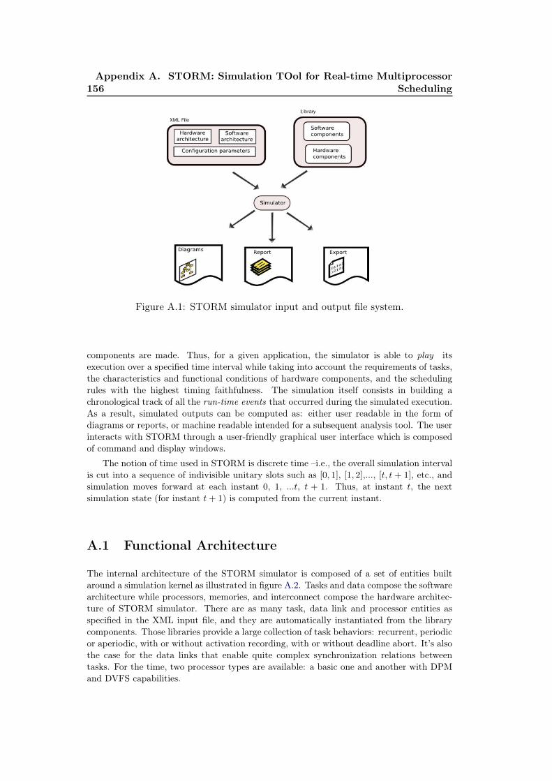
156Appendix A. STORM: Simulation TOol for Real-time Multiprocessor
Scheduling
Figure A.1: STORM simulator input and output file system.
components are made. Thus, for a given application, the simulator is able to play itsexecution over a specified time interval while taking into account the requirements of tasks,the characteristics and functional conditions of hardware components, and the schedulingrules with the highest timing faithfulness. The simulation itself consists in building achronological track of all the run-time events that occurred during the simulated execution.As a result, simulated outputs can be computed as: either user readable in the form ofdiagrams or reports, or machine readable intended for a subsequent analysis tool. The userinteracts with STORM through a user-friendly graphical user interface which is composedof command and display windows.
The notion of time used in STORM is discrete time –i.e., the overall simulation intervalis cut into a sequence of indivisible unitary slots such as [0, 1], [1, 2],..., [t, t + 1], etc., andsimulation moves forward at each instant 0, 1, ...t, t + 1. Thus, at instant t, the nextsimulation state (for instant t+ 1) is computed from the current instant.
A.1 Functional Architecture
The internal architecture of the STORM simulator is composed of a set of entities builtaround a simulation kernel as illustrated in figure A.2. Tasks and data compose the softwarearchitecture while processors, memories, and interconnect compose the hardware architec-ture of STORM simulator. There are as many task, data link and processor entities asspecified in the XML input file, and they are automatically instantiated from the librarycomponents. Those libraries provide a large collection of task behaviors: recurrent, periodicor aperiodic, with or without activation recording, with or without deadline abort. It’s alsothe case for the data links that enable quite complex synchronization relations betweentasks. For the time, two processor types are available: a basic one and another with DPMand DVFS capabilities.
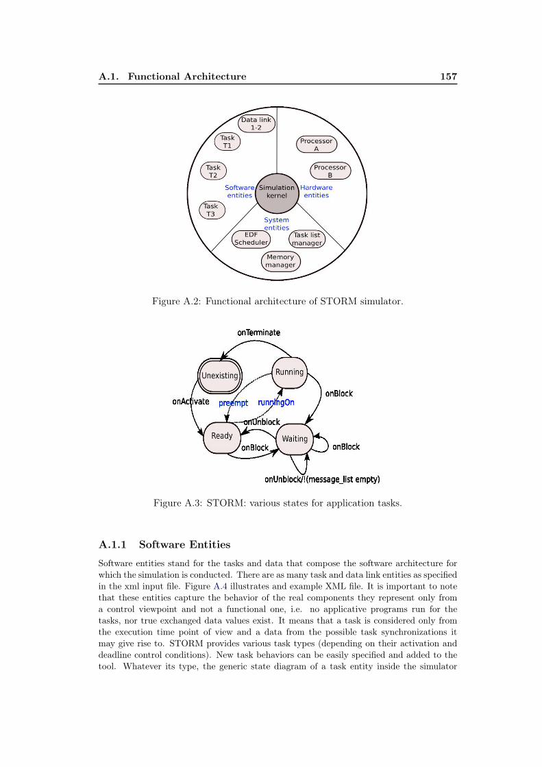
A.1. Functional Architecture 157
Figure A.2: Functional architecture of STORM simulator.
Figure A.3: STORM: various states for application tasks.
A.1.1 Software Entities
Software entities stand for the tasks and data that compose the software architecture forwhich the simulation is conducted. There are as many task and data link entities as specifiedin the xml input file. Figure A.4 illustrates and example XML file. It is important to notethat these entities capture the behavior of the real components they represent only froma control viewpoint and not a functional one, i.e. no applicative programs run for thetasks, nor true exchanged data values exist. It means that a task is considered only fromthe execution time point of view and a data from the possible task synchronizations itmay give rise to. STORM provides various task types (depending on their activation anddeadline control conditions). New task behaviors can be easily specified and added to thetool. Whatever its type, the generic state diagram of a task entity inside the simulator
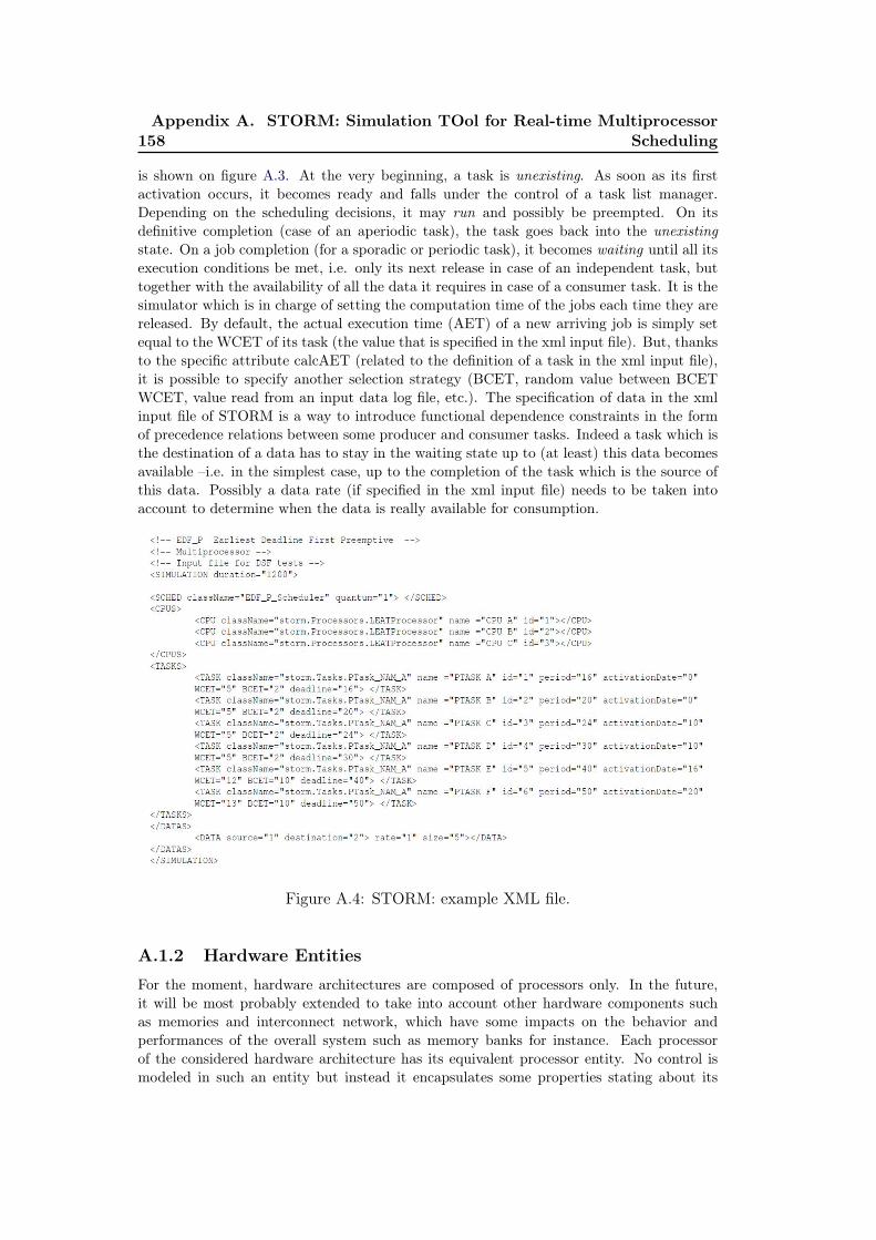
158Appendix A. STORM: Simulation TOol for Real-time Multiprocessor
Scheduling
is shown on figure A.3. At the very beginning, a task is unexisting. As soon as its firstactivation occurs, it becomes ready and falls under the control of a task list manager.Depending on the scheduling decisions, it may run and possibly be preempted. On itsdefinitive completion (case of an aperiodic task), the task goes back into the unexistingstate. On a job completion (for a sporadic or periodic task), it becomes waiting until all itsexecution conditions be met, i.e. only its next release in case of an independent task, buttogether with the availability of all the data it requires in case of a consumer task. It is thesimulator which is in charge of setting the computation time of the jobs each time they arereleased. By default, the actual execution time (AET) of a new arriving job is simply setequal to the WCET of its task (the value that is specified in the xml input file). But, thanksto the specific attribute calcAET (related to the definition of a task in the xml input file),it is possible to specify another selection strategy (BCET, random value between BCETWCET, value read from an input data log file, etc.). The specification of data in the xmlinput file of STORM is a way to introduce functional dependence constraints in the formof precedence relations between some producer and consumer tasks. Indeed a task which isthe destination of a data has to stay in the waiting state up to (at least) this data becomesavailable –i.e. in the simplest case, up to the completion of the task which is the source ofthis data. Possibly a data rate (if specified in the xml input file) needs to be taken intoaccount to determine when the data is really available for consumption.
Figure A.4: STORM: example XML file.
A.1.2 Hardware Entities
For the moment, hardware architectures are composed of processors only. In the future,it will be most probably extended to take into account other hardware components suchas memories and interconnect network, which have some impacts on the behavior andperformances of the overall system such as memory banks for instance. Each processorof the considered hardware architecture has its equivalent processor entity. No control ismodeled in such an entity but instead it encapsulates some properties stating about its

A.1. Functional Architecture 159
current activity such as running, idle, or busy. In case of a processor with DVFS (DynamicVoltage and Frequency Scaling) and DPM(Dynamic Power Management) capabilities, thecorresponding entity owns additional properties about its current functionality such aspower consumption mode, operating voltage, and frequency etc. together with the functionsfor updating them.
A.1.3 System Entities
At the moment, system entities are the task list manager, the scheduling algorithms, and thepower management policies. The part of the task list manager entity is twofold. It controlsthe very first release of each task: after a successful comparison between a task activationdate and the current time, it produces a specific activation kernel message that is relayedby the kernel towards the concerned task entity and the scheduler entity too. Moreoverit manages functional constraints between tasks that appear when data dependencies havebeen specified: at each simulation slot, depending on the availability or consumption ofdata, it produces specific task block or unblock kernel messages. The scheduler entity isin charge of sharing the processor(s) between the ready tasks. Its election rules dependon the scheduling strategy it implements. It owns proper queue(s) about ready tasks andmanages them thanks to the task state change indications the kernel sends to it and thetick indication too. The election rules it implements may lead it to run and/or to preempta task. STORM provides most of the standard real-time global event-driven or time-drivenschedulers.
A.1.4 Simulation Kernel
The behavior of simulation kernel is a cyclic one –i.e., one cycle for one slot. After anecessary initial step where all the simulation entities are created and the global timevariable is initialized, the loop of cycles is entered. Any cycle performs successive stepsthat come down to manage the watchdogs –i.e., to detect those possible watchdogs thatexpire and to call the specified function of the specified entity, process all the currentlypending kernel messages, call upon the scheduler, manage time passing, ask for the task listmanager to operate, and increment the time variable. Furthermore, all along its cycles, thekernel records all the event occurrences and associated data that are relevant for buildingthe simulation outputs.

Appendix B
HyPowMan Scheme: AdditionalSimulation Results
B.1 Simulation Results Using AsDPM & DSF Experts
In this appendix, we provide additional simulation results on HyPowMan scheme usingAsDPM technique (see chapter 4) and DSF technique (see chapter 5) together as experts.These results are obtained for the same target application and simulation settings as usedin chapter 6. We observe that the results obtained using DSF and AsDPM as experts aresimilar to the results obtained in chapter 6 as far as validating the working of HyPowManis concerned. One exception in these results is that, consistently, AsDPM technique resultsin better energy savings as compared to DSF technique against all variations –i.e., variationin bcet/wcet ratio, number of tasks, and aggregate utilization. Based on this observation,it is obvious that using only AsDPM technique in this particular case could have yieldedbest energy savings. Moreover, these results also demonstrate that if the designer/user doesnot select a single best-performing expert statically based on prior knowledge, HyPowManscheme can still converge to the single best policy in an online fashion. However, thecomputational overheads related to HyPowMan scheme could have be avoided in case ofstatically selected single expert. We have not included these results in chapter 6 as it couldhave limited the reader from understanding the full potential of HyPowMan scheme. Here,we present these results for reference.
B.1.1 Effect of variations in bcet/wcet ratio
We make the following observations on these results. For bcet/wcet ratio= 1, figure B.1depicts no change in total energy consumption due to constant dynamic and static powerconsumption. Since actual execution time remains constant, energy consumed by processorsunder non-optimized case and under DSF expert alone remains unchanged. AsDPM expertalone, however, saves energy by exploiting the presence of inherent (static) idle intervals.HyPowMan scheme, in this case, converges to AsDPM expert in a straightforward manneras shown in figure B.1. As bcet/wcet ratio decreases (< 1), opportunities for DSF expertto save energy are created as well. Figure B.1 shows that both DSF and AsDPM experts,while working alone, save energy as compared to non-optimized case. For bcet/wcet ratiobetween 0.5 and 0.9, HyPowMan scheme converges to the best energy savings offered byeither expert.
B.1.2 Effect of variations in number of tasks
Similar to the settings in section 6.4.3.2, we double and triple the number of tasks. Resultsin figure B.2 depict that, increasing the number of tasks increases the energy savings inall cases. These results are very much similar to those obtained in section 6.4.3.2 with theexception that AsDPM expert performed better than DSF expert in all cases.
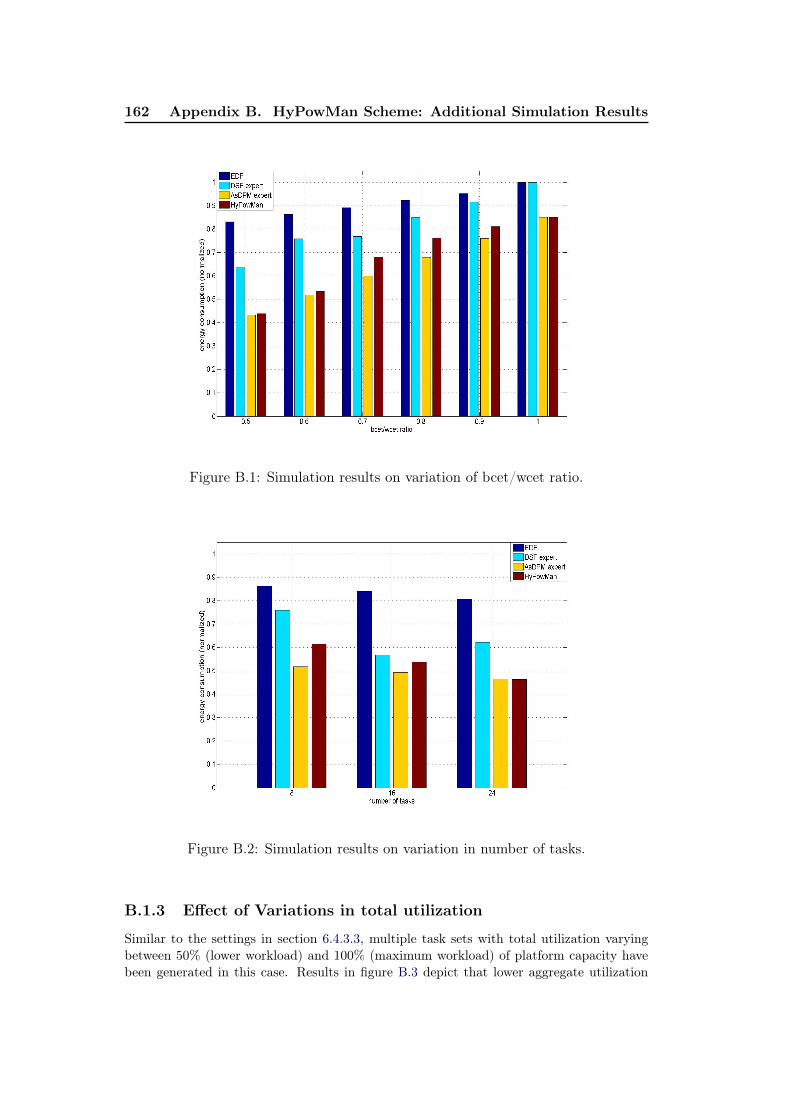
162 Appendix B. HyPowMan Scheme: Additional Simulation Results
Figure B.1: Simulation results on variation of bcet/wcet ratio.
Figure B.2: Simulation results on variation in number of tasks.
B.1.3 Effect of Variations in total utilization
Similar to the settings in section 6.4.3.3, multiple task sets with total utilization varyingbetween 50% (lower workload) and 100% (maximum workload) of platform capacity havebeen generated in this case. Results in figure B.3 depict that lower aggregate utilization
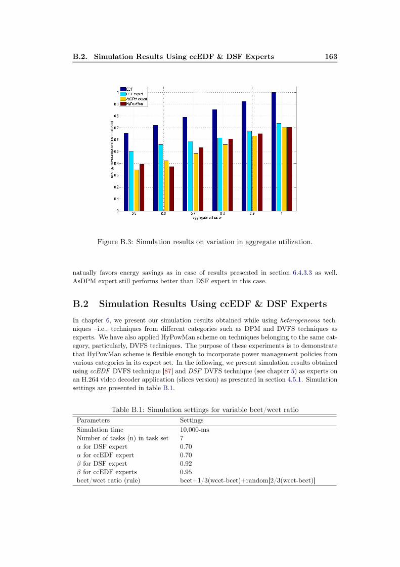
B.2. Simulation Results Using ccEDF & DSF Experts 163
Figure B.3: Simulation results on variation in aggregate utilization.
natually favors energy savings as in case of results presented in section 6.4.3.3 as well.AsDPM expert still performs better than DSF expert in this case.
B.2 Simulation Results Using ccEDF & DSF Experts
In chapter 6, we present our simulation results obtained while using heterogeneous tech-niques –i.e., techniques from different categories such as DPM and DVFS techniques asexperts. We have also applied HyPowMan scheme on techniques belonging to the same cat-egory, particularly, DVFS techniques. The purpose of these experiments is to demonstratethat HyPowMan scheme is flexible enough to incorporate power management policies fromvarious categories in its expert set. In the following, we present simulation results obtainedusing ccEDF DVFS technique [87] and DSF DVFS technique (see chapter 5) as experts onan H.264 video decoder application (slices version) as presented in section 4.5.1. Simulationsettings are presented in table B.1.
Table B.1: Simulation settings for variable bcet/wcet ratioParameters SettingsSimulation time 10,000-msNumber of tasks (n) in task set 7α for DSF expert 0.70α for ccEDF expert 0.70β for DSF expert 0.92β for ccEDF experts 0.95bcet/wcet ratio (rule) bcet+1/3(wcet-bcet)+random[2/3(wcet-bcet)]
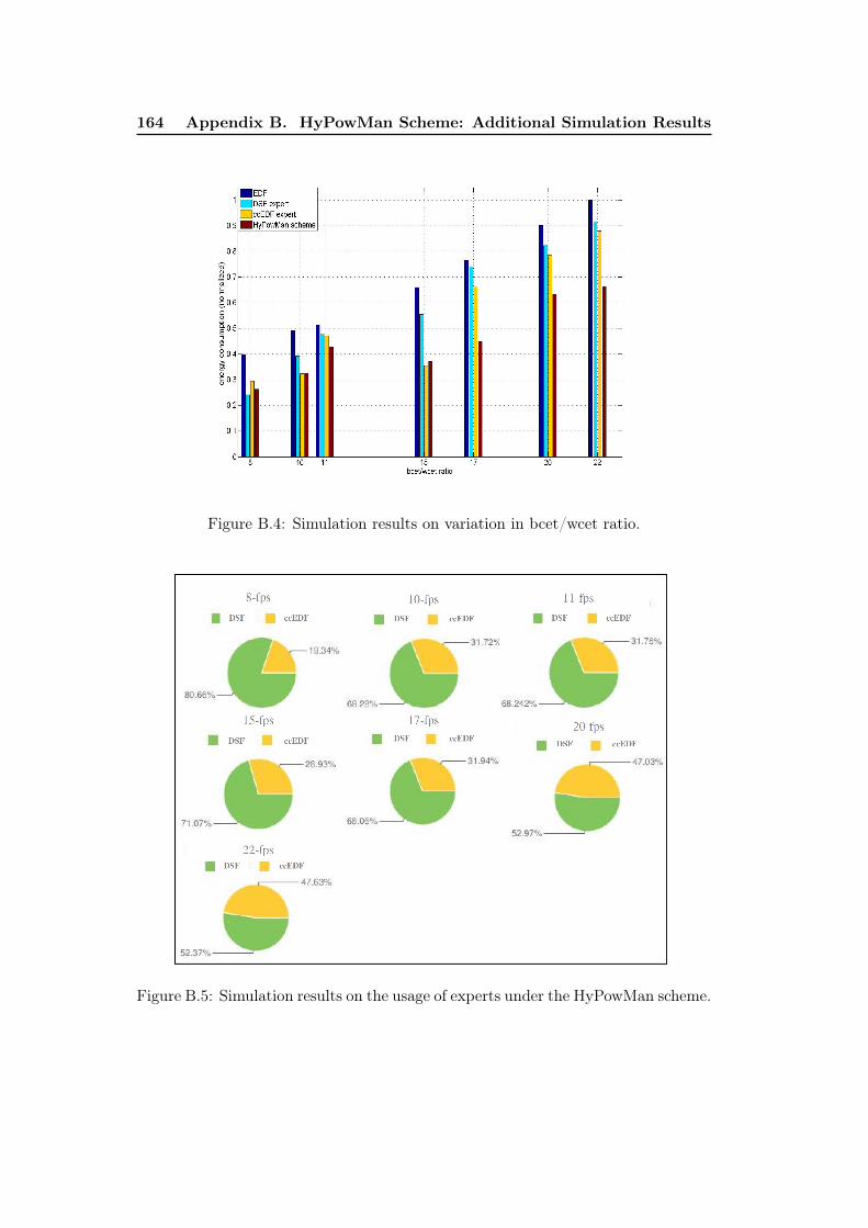
164 Appendix B. HyPowMan Scheme: Additional Simulation Results
Figure B.4: Simulation results on variation in bcet/wcet ratio.
Figure B.5: Simulation results on the usage of experts under the HyPowMan scheme.
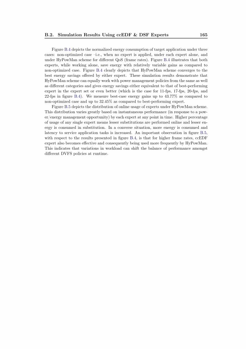
B.2. Simulation Results Using ccEDF & DSF Experts 165
Figure B.4 depicts the normalized energy consumption of target application under threecases: non-optimized case –i.e., when no expert is applied, under each expert alone, andunder HyPowMan scheme for different QoS (frame rates). Figure B.4 illustrates that bothexperts, while working alone, save energy with relatively variable gains as compared tonon-optimized case. Figure B.4 clearly depicts that HyPowMan scheme converges to thebest energy savings offered by either expert. These simulation results demonstrate thatHyPowMan scheme can equally work with power management policies from the same as wellas different categories and gives energy savings either equivalent to that of best-performingexpert in the expert set or even better (which is the case for 11-fps, 17-fps, 20-fps, and22-fps in figure B.4). We measure best-case energy gains up to 43.77% as compared tonon-optimized case and up to 32.45% as compared to best-performing expert.
Figure B.5 depicts the distribution of online usage of experts under HyPowMan scheme.This distribution varies greatly based on instantaneous performance (in response to a pow-er/energy management opportunity) by each expert at any point in time. Higher percentageof usage of any single expert means lesser substitutions are performed online and lesser en-ergy is consumed in substitution. In a converse situation, more energy is consumed andlatency to service application tasks is increased. An important observation in figure B.5,with respect to the results presented in figure B.4, is that for higher frame rates, ccEDFexpert also becomes effective and consequently being used more frequently by HyPowMan.This indicates that variations in workload can shift the balance of performance amongstdifferent DVFS policies at runtime.

Bibliography
[1] Tarek A. AlEnawy and Hakan Aydin. Energy-aware task allocation for rate monotonicscheduling. In procs. of IEEE Symposium, RTAS-2005, pages 213–223, 2005. 115
[2] AMD. AMD Technical Docs, 2010. http://support.amd.com. 85
[3] James H. Anderson and Sanjoy K. Baruah. Energy-aware implementation of hard-real-time systems upon multiprocessor platforms. In In Proceedings of the ISCA16th International Conference on Parallel and Distributed Computing Systems, pages430–435, 2002. 12, 17
[4] James H. Anderson and Sanjoy K. Baruah. Energy-efficient synthesis of periodictask systems upon identical multiprocessor platforms. In Proceedings of the 24thInternational Conference on Distributed Computing Systems (ICDCS’04), ICDCS ’04,pages 428–435, Washington, DC, USA, 2004. IEEE Computer Society. 17
[5] James H. Anderson, Vasile Bud, and UmaMaheswari C. Devi. An edf-based schedul-ing algorithm for multiprocessor soft real-time systems. In Proceedings of the 17thEuromicro Conference on Real-Time Systems, pages 199–208, Washington, DC, USA,2005. IEEE Computer Society. 35
[6] James H. Anderson and Anand Srinivasan. Mixed pfair/erfair scheduling of asyn-chronous periodic tasks. In Proceedings of the 13th Euromicro Conference on Real-Time Systems, ECRTS ’01, pages 76–, Washington, DC, USA, 2001. IEEE ComputerSociety. 54
[7] Bjorn Andersson, Sanjoy Baruah, and Jan Jonsson. Static-priority scheduling onmultiprocessors. In Proceedings of the 22nd IEEE Real-Time Systems Symposium,RTSS ’01, pages 93–, Washington, DC, USA, 2001. IEEE Computer Society. 22, 35,39
[8] Bjorn Andersson and Eduardo Tovar. Multiprocessor scheduling with few preemp-tions. In Proceedings of the 12th IEEE International Conference on Embedded andReal-Time Computing Systems and Applications, RTCSA ’06, pages 322–334, Wash-ington, DC, USA, 2006. IEEE Computer Society. 20, 22, 32, 33, 34
[9] ARM. ARM Architecture, 2010. http://www.arm.com/. 85, 130, 150
[10] Hakan Aydin, Rami Melhem, Daniel Mossé, and Pedro Mejía-Alvarez. Power-awarescheduling for periodic real-time tasks. IEEE Trans. Comput., 53:584–600, May 2004.8, 28, 77, 86, 87, 89, 98, 99, 105, 116, 128, 139, 146, 149
[11] Hakan AYDIN, Rami MELHEM, Daniel MOSSÉ, and P. MEJIA-ALVAREZ. Power-aware scheduling for periodic real-time tasks. In IEEE Transactions on Computers,pages 584 – 600. IEEE, vol. 53, n◦5, 2004. 51
[12] Hakan Aydin and Qi Yang. Energy-aware partitioning for multiprocessor real-timesystems. In Proceedings of the 17th International Symposium on Parallel and Dis-tributed Processing, IPDPS ’03, pages 113.2–, Washington, DC, USA, 2003. IEEEComputer Society. 89
[13] Sanjoy Baruah, Neil Cohen, Greg Plaxton, and Don Varvel. Proportionate progress:A notion of fairness in resource allocation. In Algorithmica, page 600 625, 1996. 4,31, 35, 129, 136, 149
168 Bibliography
[14] Sanjoy K. Baruah, N. K. Cohen, C. G. Plaxton, and D. A. Varvel. Proportionateprogress: a notion of fairness in resource allocation. In Proceedings of the twenty-fifthannual ACM symposium on Theory of computing, STOC ’93, pages 345–354, NewYork, NY, USA, 1993. ACM. 52
[15] Sanjoy K. Baruah, Aloysius K. Mok, and Louis E. Rosier. Preemptively schedulinghard-real-time sporadic tasks on one processor. In In Proceedings of the 11th Real-Time Systems Symposium, pages 182–190. IEEE Computer Society Press, 1990. 44
[16] Luca Benini, Alessandro Bogliolo, and Giovanni De Micheli. A survey of designtechniques for system-level dynamic power management. In Giovanni De Micheli,Rolf Ernst, and Wayne Wolf, editors, Readings in hardware/software co-design, pages231–248. Kluwer Academic Publishers, Norwell, MA, USA, 2002. 26, 58, 60
[17] Luca Benini and Giovanni de Micheli. Dynamic Power Management: Design Tech-niques and CAD Tools. Springer, 1997. 26
[18] Luca Benini and Giovanni De Micheli. Dynamic Power Management: Design Tech-niques and CAD Tools. Springer; 1st edition (November 30, 1997), 1997. 60
[19] Muhammad Khurram Bhatti, Cécile Belleudy, and Michel Auguin. An inter-task realtime dvfs scheme for multiprocessor embedded systems. In Proceedings of IEEE in-ternational conference on Design and Architectures for Signal and Image Processing,DASIP, 2010. 115
[20] Muhammad Khurram Bhatti, Cécile Belleudy, and Michel Auguin. Power manage-ment in real time embedded systems through online and adaptive interplay of dpmand dvfs policies. In proceedings of International Conference on Embedded and Ubiq-uitous Computing, EUC’10, EUC’10, 2010. 8, 140, 146
[21] Enrico Bini, Giorgio C. Buttazzo, and Giuseppe M. Buttazzo. Rate monotonic anal-ysis: The hyperbolic bound. IEEE Trans. Comput., 52:933–942, July 2003. 20
[22] Enrico Bini, Giorgio C. Buttazzo, and Giuseppe Lipari. Speed modulation in energy-aware real-time systems. In IEEE Proceedings of the Euromicro Conference on Real-Time Systems, ECRTS, 2005. 99
[23] Alan Burns and Andy Wellings. Real-Time Systems and Programming Languages(Third Edition). Ada 95, Real-Time Java and Real-Time POSIX. Hardback - 611pages. Addison Wesley Longmain, 2001. 19, 22
[24] John M. Calandrino, James H. Anderson, and Dan P. Baumberger. A hybrid real-time scheduling approach for large-scale multicore platforms. In Proceedings of the19th Euromicro Conference on Real-Time Systems, ECRTS’07, pages 247–256, 2007.32, 34, 35, 124, 144
[25] Jian-Jia Chen and Chin-Fu Kuo. Energy-efficient scheduling for real-time systems ondynamic voltage scaling (dvs) platforms. In Proceedings of the 13th IEEE Interna-tional Conference on Embedded and Real-Time Computing Systems and Applications,RTCSA ’07, pages 28–38, Washington, DC, USA, 2007. IEEE Computer Society. 89
[26] Hui Cheng and Steve Goddard. Online energy-aware i/o device scheduling for hardreal-time systems. In Proceedings of the conference on Design, automation and test inEurope: Proceedings, DATE ’06, pages 1055–1060, 3001 Leuven, Belgium, Belgium,2006. European Design and Automation Association. 60

Bibliography 169
[27] Hui Cheng and Steve Goddard. Sys-edf: a system-wide energy-efficient schedulingalgorithm for hard real-time systems. In International Journal of Embedded Systems,pages 141 – 151. Inderscience, Volume 4, Number 2 / 2009, 2009. 60, 79, 82, 109
[28] Hyeonjoong Cho, Binoy Ravindran, and E. Douglas Jensen. An optimal real-timescheduling algorithm for multiprocessors. In Proceedings of the 27th IEEE Interna-tional Real-Time Systems Symposium, pages 101–110, Washington, DC, USA, 2006.IEEE Computer Society. 4, 31, 52, 129, 136, 149
[29] Eui-Young Chung, Luca Benini, Alessandro Bogiolo, and Giovanni De Micheli. Dy-namic power management for non-stationary service requests. In Proceedings of theconference on Design, automation and test in Europe, DATE ’99, New York, NY,USA, 1999. ACM. 27, 60
[30] Ayse K. Coskun, David Atienza, Tajana Simunic Rosing, Thomas Brunschwiler, andBruno Michel. Energy-efficient variable-flow liquid cooling in 3d stacked architectures.In Proceedings of the Conference on Design, Automation and Test in Europe, DATE’10, pages 111–116, 3001 Leuven, Belgium, Belgium, 2010. European Design andAutomation Association. 5, 130, 136, 150
[31] Victor De La Luz, Mahmut Kandemir, and Ugur Sezer. Improving off-chip memoryenergy behavior in a multi-processor, multi-bank environment. In Proceedings ofthe 14th international conference on Languages and compilers for parallel computing,LCPC’01, pages 100–114, Berlin, Heidelberg, 2003. Springer-Verlag. 80
[32] V. Delaluz, M. Kandemir, N. Vijaykrishnan, A. Sivasubramaniam, and M. J. Irwin.Dram energy management using sof ware and hardware directed power mode control.In Proceedings of the 7th International Symposium on High-Performance ComputerArchitecture, HPCA ’01, pages 159–, Washington, DC, USA, 2001. IEEE ComputerSociety. 80
[33] M. L. Dertouzos and A. K. Mok. Multiprocessor online scheduling of hard-real-timetasks. IEEE Trans. Softw. Eng., 15:1497–1506, December 1989. 19
[34] Michael Dertouzos and Aloysius Mok. Multiprocessor scheduling in a hard real-timeenvironment. In IEEE Transactions on Software Engineering, page 1497 1506, 1989.22, 35
[35] Vinay Devadas and Hakan Aydin. On the interplay of dynamic voltage scaling anddynamic power management in real-time embedded applications. In Proceedings ofthe 8th ACM international conference on Embedded software, EMSOFT ’08, pages99–108, New York, NY, USA, 2008. ACM. 27, 59, 60, 109
[36] Vinay Devadas and Hakan Aydin. Real-time dynamic power management throughdevice forbidden regions. In Proceedings of the 2008 IEEE Real-Time and EmbeddedTechnology and Applications Symposium, pages 34–44, Washington, DC, USA, 2008.IEEE Computer Society. 59, 60
[37] Gaurav Dhiman and Tajana Simunic Rosing. Dynamic power management usingmachine learning. In Proceedings of the 2006 IEEE/ACM international conferenceon Computer-aided design, ICCAD ’06, pages 747–754, New York, NY, USA, 2006.ACM. 8, 108, 109, 110, 140, 146
[38] Francois Dorin, Patrick Meumeu Yomsi, Joel Goossens, and Pascal Richard. Semi-partitioned hard real-time scheduling with restricted migrations upon identical multi-processor platforms. In Operating Systems (cs.OS), arXiv:1006.2637v1 [cs.OS], Cor-nell University Library Archives, Technical Report, June, 2010. 34, 35, 36, 37
170 Bibliography
[39] R. ERNST and W. YE. Embedded program timing analysis based on path clusteringand architecture classification. In the proceedings of International Conference onComputer-Aided Design (ICCAD 97), pages 598 – 604, 1997. 50, 90
[40] Rolf Ernst and Weisong Ye. Embedded program timing analysis based on path clus-tering and architecture classification. In Proceedings of the 1997 IEEE/ACM interna-tional conference on Computer-aided design, ICCAD ’97, pages 598–604, Washington,DC, USA, 1997. IEEE Computer Society. 28, 86
[41] Amir H. Farrahi, Gustavo E. Téllez, and Majid Sarrafzadeh. Memory segmentation toexploit sleep mode operation. In Proceedings of the 32nd annual ACM/IEEE DesignAutomation Conference, DAC ’95, pages 36–41, New York, NY, USA, 1995. ACM.80
[42] Nathan Wayne Fisher. The Multiprocessor Real-Time Scheduling of General TaskSystems, 2007. PhD Thesis, University of North-Carolina at Chapel Hill,. 3, 11, 18,20, 135
[43] Yoav Freund and Robert E. Schapire. A decision-theoretic generalization of on-linelearning and an application to boosting. In Proceedings of the Second European Con-ference on Computational Learning Theory, pages 23–37, London, UK, 1995. Springer-Verlag. 110
[44] Kenji Funaoka, Shinpei Kato, and Nobuyuki Yamasaki. A context cache replacementalgorithm for pfair scheduling. In Proceedings of the 15th International Conferenceon Real-Time and Network Systems (RTNS), pages 57 – 64, 2007. 46
[45] Kenji Funaoka, Shinpei Kato, and Nobuyuki Yamasaki. Dynamic voltage and fre-quency scaling for optimal real-time scheduling on multiprocessors. In Proceedingsof Industrial Embedded Systems, 2008. SIES 2008. International Symposium, pages27–33, Le Grande Motte, France, 2008. 89
[46] Kenji Funaoka, Shinpei Kato, and Nobuyuki Yamasaki. Energy-efficient optimal real-time scheduling on multiprocessors. In Proceedings of the 2008 11th IEEE Symposiumon Object Oriented Real-Time Distributed Computing, pages 23–30, Washington, DC,USA, 2008. IEEE Computer Society. 89, 90, 108
[47] Shelby Hyatt Funk. Edf scheduling on heterogeneous multiprocessors. In PhD thesis,department of computer science. University of North Carolina at Chapel Hill, 2004.3, 11, 18, 20, 22, 135
[48] Bruno Gaujal and Nicolas Navet. Dynamic voltage scaling under edf revisited. Real-Time Syst., 37:77 – 97, October 2007. 28, 85, 125, 145
[49] S. Gochman, R. Ronen, I. Anati, A. Berkovis, T. Kurts, A. Naveh, A. Saeed, Z. Sper-ber, and R. C. Valentine. The intel pentium m processor: Microarchitecture andperformance. In Proceedings of Intel Technology Journal, Vol. 7, Issue 2, pages 21–36, 2003. 89
[50] Flavius Gruian. System-level design methods for low-energy architectures containingvariable voltage processors. In Proceedings of the First International Workshop onPower-Aware Computer Systems-Revised Papers, PACS ’00, pages 1–12, London, UK,2001. Springer-Verlag. 89
[51] Flavius GRUIAN. Energy-centric scheduling for real-time systems. In PhD thesis.http://www.cs.lth.se/home/Flavius Gruian, 2002. 86
Bibliography 171
[52] Kwang Soo Hong and Joseph Y.-T. Leung. On-line scheduling of real-time tasks. InIEEE Real-Time Systems Symposium, page 244 250, Huntsville,Alabama, 1988. 22,35
[53] Chi-Hong Hwang and Allen C.-H. Wu. A predictive system shutdown method forenergy saving of event-driven computation. ACM Trans. Des. Autom. Electron. Syst.,5:226–241, April 2000. 58
[54] Intel. Intel Technical Docs, 2010. http://www.intel.com. 85
[55] S. Irani, R. Gupta, and S. Shukla. Competitive analysis of dynamic power manage-ment strategies for systems with multiple power savings states. In Proceedings ofthe conference on Design, automation and test in Europe, DATE ’02, pages 117–,Washington, DC, USA, 2002. IEEE Computer Society. 27, 60
[56] Sandy Irani and Kirk R. Pruhs. Algorithmic problems in power management.SIGACT News, 36:63–76, June 2005. 4, 136
[57] Sandy Irani, Sandeep Shukla, and Rajesh Gupta. Online strategies for dynamic powermanagement in systems with multiple power-saving states. ACM Trans. Embed.Comput. Syst., 2:325–346, August 2003. 26, 57, 60
[58] Ravindra Jejurikar and Rajesh Gupta. Dynamic voltage scaling for systemwide energyminimization in real-time embedded systems. In Proceedings of the 2004 internationalsymposium on Low power electronics and design, ISLPED ’04, pages 78–81, New York,NY, USA, 2004. ACM. 79, 109
[59] Ravindra Jejurikar, Cristiano Pereira, and Rajesh Gupta. Leakage aware dynamicvoltage scaling for real-time embedded systems. In Proceedings of the 41st annualDesign Automation Conference, DAC ’04, pages 275–280, New York, NY, USA, 2004.ACM. 90
[60] David Johnson. Near-optimal bin packing algorithms. In PhD thesis, Department ofMathematics, Massachusetts Institute of Technology, 1973. 4, 6, 32, 124, 136, 138,144
[61] Anna R. Karlin, Mark S. Manasse, Lyle A. McGeoch, and Susan Owicki. Compet-itive randomized algorithms for non-uniform problems. In Proceedings of the firstannual ACM-SIAM symposium on Discrete algorithms, SODA ’90, pages 301–309,Philadelphia, PA, USA, 1990. Society for Industrial and Applied Mathematics. 115
[62] Shinpei Kato and Nobuyuki Yamasaki. Portioned edf-based scheduling on multi-processors. In Proceedings of the 8th ACM international conference on Embeddedsoftware, EMSOFT ’08, pages 139–148, New York, NY, USA, 2008. ACM. 32, 33, 34,35, 36, 37, 124, 144
[63] Shinpei Kato, Nobuyuki Yamasaki, and Yutaka Ishikawa. Semi-partitioned schedulingof sporadic task systems on multiprocessors. In Proceedings of the 2009 21st Euromi-cro Conference on Real-Time Systems, pages 249–258, Washington, DC, USA, 2009.IEEE Computer Society. 20, 32, 33, 34, 44, 124, 144
[64] Minyoung Kim and Soonhoi Ha. Hybrid run-time power management technique forreal-time embedded system with voltage scalable processor. In Proceedings of the 2001ACM SIGPLAN workshop on Optimization of middleware and distributed systems,OM ’01, pages 11–19, New York, NY, USA, 2001. ACM. 109
172 Bibliography
[65] C. M. Krishna and Yann-Hang Lee. Voltage-clock-scaling adaptive scheduling tech-niques for low power in hard real-time systems. IEEE Trans. Comput., 52:1586–1593,December 2003. 89
[66] Woo-Cheol Kwon and Taewhan Kim. Optimal voltage allocation techniques for dy-namically variable voltage processors. In Proceedings of the 40th annual Design Au-tomation Conference, DAC ’03, pages 125–130, New York, NY, USA, 2003. ACM.89
[67] Alvin R. Lebeck, Xiaobo Fan, Heng Zeng, and Carla Ellis. Power aware page alloca-tion. SIGARCH Comput. Archit. News, 28:105–116, November 2000. 80
[68] Seongsoo Lee and Takayasu Sakurai. Run-time voltage hopping for low-power real-time systems. In Proceedings of the 37th Annual Design Automation Conference,DAC ’00, pages 806–809, New York, NY, USA, 2000. ACM. 28
[69] Benjamin Lesage, Damien Hardy, and Isabelle Puaut. Shared data cache conflictsreduction for wcet computation in multi-core architectures. In Proceedings of 18thInternational Conference on Real-Time and Network Systems, Toulouse, France, 2010.14
[70] Benjamin Lesage and Isabelle Puaut. Estimation of cache related migration delays formulti-core processors with shared instruction caches. In Proceedings of 17th Interna-tional Conference on Real-Time and Network Systems, pages 45 – 54, Paris, France,2009. 14
[71] Chung L. Liu and James W. Layland. Scheduling algorithms for multiprogrammingin a hard-real-time environment. Journal of ACM, 20:46–61, January 1973. 15, 19,20, 22, 129, 149
[72] Marvell. Marvell’s XScale Microarchitecture. http://www.marvell.com/. 29, 85
[73] Andreas Merkel and Frank Bellosa. Balancing power consumption in multiprocessorsystems. SIGOPS Oper. Syst. Rev., 40:403–414, April 2006. 82, 84
[74] Aloysius K. Mok. Task management techniques for enforcing ed scheduling on aperiodic task set. Proceedings of 5th IEEE Workshop on Real-Time Software andOperating Systems, pages 42–46, 1988. 22
[75] Daniel Mosse, Hakan Aydin, Bruce Childers, and Rami Melhem. Compiler-assisteddynamic power-aware scheduling for real-time applications. In In Workshop on Com-pilers and Operating Systems for Low Power, 2000. 89
[76] Daniel MOSSE, Hakan AYDIN, Buce CHILDERS, and Rami MELHEM. Compiler-assisted dynamic power-aware scheduling for real-time applications. In Workshop onCompiler and Operating Sys for Low-Power, 2000. 86
[77] Farooq Muhammad. Ordonnancement de tâches efficace et â complexitè maîtrisèepour des systèmes temps rèel. In PhD thesis. University of Nice-Sophia Antipolis,2009. 3, 4, 11, 31, 37, 44, 52, 54, 135, 136
[78] Fabrizio Mulas, David Atienza, Andrea Acquaviva, Salvatore Carta, Luca Benini, andGiovanni De Micheli. Thermal balancing policy for multiprocessor stream computingplatforms. Trans. Comp.-Aided Des. Integ. Cir. Sys., 28:1870–1882, December 2009.79, 82, 130
Bibliography 173
[79] N. NAVET and B. GAUJAL. Ordonnancement temps reel et minimisation de laconsommation de energie. Chapter-4 in System Temps Reel -Volume 2. Kluwer Pub-lishers, 2006. 26, 86, 87
[80] Vincent Nelis. Energy-Aware Real-Time Scheduling in Embedded MultiprocessorSystems, 2010. PhD Thesis, Université Libre de Bruxelles, Belgium. 11, 25
[81] Ozcan Ozturk and Mahmut Kandemir. Nonuniform banking for reducing memoryenergy consumption. In Proceedings of the conference on Design, Automation andTest in Europe - Volume 2, DATE ’05, pages 814–819, Washington, DC, USA, 2005.IEEE Computer Society. 80
[82] Ozcan Ozturk, Mahmut Kandemir, and I. Koleu. Reducing memory energy consump-tion of embedded applications that process dynamically allocated data. In IEEEtransactions on computer-aided design of integrated circuits and systems, vol. 25,no.9, 2006. 80
[83] G. A. Paleologo, L. Benini, A. Bogliolo, and G. De Micheli. Policy optimization fordynamic power management. In Proceedings of the 35th annual Design AutomationConference, DAC ’98, pages 182–187, New York, NY, USA, 1998. ACM. 26, 60
[84] G. A. Paleologo, L. Benini, A. Bogliolo, and G. De Micheli. Policy optimization fordynamic power management. In Proceedings of the 35th annual Design AutomationConference, DAC ’98, pages 182–187, New York, NY, USA, 1998. ACM. 60
[85] Minkyu Park, Sangchul Han, Heeheon Kim, Seongje Cho, and Yookun Cho. Com-parison of deadline-based scheduling algorithms for periodic real-time tasks on mul-tiprocessor*this work is supported in part by brain korea 21 project and in part byict. IEICE - Trans. Inf. Syst., E88-D:658–661, March 2005. 19
[86] PHERMA. ANR project Pherma (Reference: ANR-06-ARFU06-003) , 2007 - 2010.http://pherma.irccyn.ec-nantes.fr. 28, 70, 128, 148, 155
[87] Padmanabhan Pillai and Kang G. Shin. Real-time dynamic voltage scaling for low-power embedded operating systems. In Proceedings of the eighteenth ACM symposiumon Operating systems principles, SOSP ’01, pages 89–102, New York, NY, USA, 2001.ACM. 28, 89, 102, 115, 163
[88] Pherma project technical report. Validation of the offline and online optimizationtools, 2010. http://pherma.irccyn.ec-nantes.fr/publications.php. 29, 69, 102, 103,105
[89] QEMU. QEMU, 2010. http://wiki.qemu.org/. 105, 130, 150
[90] Qinru Qiu and Massoud Pedram. Dynamic power management based on continuous-time markov decision processes. In Proceedings of the 36th annual ACM/IEEE DesignAutomation Conference, DAC ’99, pages 555–561, New York, NY, USA, 1999. ACM.60
[91] Gang Quan and Xiaobo Sharon Hu. Energy efficient dvs schedule for fixed-priorityreal-time systems. ACM Trans. Embed. Comput. Syst., 6, September 2007. 89
[92] Dinesh Ramanathan, Sandy Irani, and Rajesh Gupta. Latency effects of system levelpower management algorithms. In Proceedings of the 2000 IEEE/ACM internationalconference on Computer-aided design, ICCAD ’00, pages 350–356, Piscataway, NJ,USA, 2000. IEEE Press. 26, 27
174 Bibliography
[93] Rambus. Rambus Inc.,, 1999. http://www.rambus.com/. 80
[94] Saowanee Saewong and Ragunathan Rajrajkumar. Optimal static voltage-scaling forreal-time systems, 2007. 89
[95] Jaewon Seo, Taewhan Kim, and Ki-Seok Chung. Profile-based optimal intra-taskvoltage scheduling for hard real-time applications. In Proceedings of the 41st annualDesign Automation Conference, DAC ’04, pages 87–92, New York, NY, USA, 2004.ACM. 86
[96] Dongkun Shin and Jihong Kim. Optimizing intra-task voltage scheduling using dataflow analysis. In Proceedings of the 2005 Asia and South Pacific Design AutomationConference, ASP-DAC ’05, pages 703–708, New York, NY, USA, 2005. ACM. 86
[97] Youngsoo Shin and Kiyoung Choi. Power conscious fixed priority scheduling for hardreal-time systems. In Proceedings of the 36th annual ACM/IEEE Design AutomationConference, DAC ’99, pages 134–139, New York, NY, USA, 1999. ACM. 89, 98
[98] Youngsoo Shin, Kiyoung Choi, and Takayasu Sakurai. Power optimization of real-time embedded systems on variable speed processors. In Proceedings of the 2000IEEE/ACM international conference on Computer-aided design, ICCAD ’00, pages365–368, Piscataway, NJ, USA, 2000. IEEE Press. 86, 89
[99] Patrick M. Shriver, Maya B. Gokhale, Scott D. Briles, Dong-In Kang, Michael Cai,Kevin McCabe, Stephen P. Crago, and Jinwoo Suh. A power-aware, satellite-basedparallel signal processing scheme, pages 243–259. Kluwer Academic Publishers, Nor-well, MA, USA, 2002. 89
[100] Sandeep K. Shukla and Rajesh K. Gupta. A model checking approach to evaluatingsystem level dynamic power management policies for embedded systems. In Proceed-ings of the Sixth IEEE International High-Level Design Validation and Test Workshop(HLDVT’01), HLDVT ’01, pages 53–, Washington, DC, USA, 2001. IEEE ComputerSociety. 27, 60
[101] Tajana Simunic, Luca Benini, Andrea Acquaviva, Peter Glynn, and GiovanniDe Micheli. Dynamic voltage scaling and power management for portable systems.In Proceedings of the 38th annual Design Automation Conference, DAC ’01, pages524–529, New York, NY, USA, 2001. ACM. 109
[102] Pushkar Singh and Vinay Chinta. Survey report on dynamic power management.In Survey report of the University of Illinois, Chicago (ECE Department), Chicago,USA, 2008. 26, 58, 59
[103] Kevin Skadron, Mircea R. Stan, Karthik Sankaranarayanan, Wei Huang, SivakumarVelusamy, and David Tarjan. Temperature-aware microarchitecture: Modeling andimplementation. ACM Trans. Archit. Code Optim., 1:94–125, March 2004. 4, 136
[104] Arvind Sridhar, Alessandro Vincenzi, Martino Ruggiero, Thomas Brunschwiler, andDavid Atienza Alonso. 3d-ICE: Fast compact transient thermal modeling for 3D-ICswith inter-tier liquid cooling. In Proceedings of the 2010 (ICCAD 2010), volume 1,pages 463–470, New York, 2010. ACM and IEEE Press. 5, 130, 136, 150
[105] Anand Srinivasan. Efficient and flexible fair scheduling of real-time tasks on multipro-cessors. In PhD thesis, department of computer science. University of North Carolinaat Chapel Hill, 2003. 3, 4, 11, 135, 136
Bibliography 175
[106] Anand Srinivasan and James Anderson. Fair scheduling of dynamic task systems onmultiprocessors. J. Syst. Softw., 77:67 – 80, July 2005. 4, 35, 136
[107] Mani B. Srivastava, Anantha P. Chandrakasan, and R. W. Brodersen. Predictivesystem shutdown and other architectural techniques for energy efficient programmablecomputation. IEEE Trans. Very Large Scale Integr. Syst., 4:42–55, March 1996. 58
[108] STORM. STORM simulation tool. http://storm.rts-software.org. 8, 28, 47, 69, 99,129, 140, 150, 155
[109] Vishnu Swaminathan and Krishnendu Chakrabarty. Energy-conscious, deterministici/o device scheduling in hard . . . IEEE TRANSACTIONS ON COMPUTER-AIDEDDESIGN OF INTEGRATED CIRCUITS AND SYSTEMS, 22(7):858, 2003. 59
[110] Vishnu Swaminathan and Krishnendu Chakrabarty. Pruning-based, energy-optimal,deterministic i/o device scheduling for hard real-time systems. ACM Trans. Embed.Comput. Syst., 4:141–167, February 2005. 59, 61
[111] Vishnu Swaminathan and Krishnendu Chakrabarty. Pruning-based, energy-optimal,deterministic i/o device scheduling for hard real-time systems. ACM Trans. Embed.Comput. Syst., 4:141–167, February 2005.
[112] Vishnu Swaminathan, Krishnendu Chakrabarty, and S. S. Iyengar. Dynamic i/opower management for hard real-time systems, 2001. 59
[113] Vishnu Swaminathan, Krishnendu Chakrabarty, and S. S. Iyengar. Dynamic i/opower management for hard real-time systems. In Proceedings of the ninth interna-tional symposium on Hardware/software codesign, CODES ’01, pages 237–242, NewYork, NY, USA, 2001. ACM. 60
[114] Pengliu Tan, Jian Shu, and Zhenhua Wu. A hybrid real-time scheduling approach onmulti-core architectures. In Journal of software, vol. 5, No. 9, September 2010, pages958–965. Academy Publisher, 2010. 34
[115] Thales. Thales group (France), 2010. http://www.thalesgroup.com/. 70, 72, 104, 126
[116] Real time systems group. IRCyN research laboratory, University of Nantes, France.,2009. 28, 155
[117] Transmeta. Transmera. http://www.transmeta.com/. 85
[118] Richard Urunuela, Anne-Marie Déplanche, and Yvon Trinquet. Simulation for multi-processor real-time scheduling evaluation. In Proceedings of 7th EUROSIM Congresson Modelling and Simulation, Eurosim’10, 2010. 155
[119] Richard Urunuela, Anne-Marie Déplanche, and Yvon Trinquet. Storm: A simula-tion tool for real-time multiprocessor scheduling evaluation. In Proceedings of 15thIEEE International Conference on Emerging Technologies and Factory Automation,ETFA’10, 2010. 155
[120] Nicolas Ventroux and Raphaël David. Scmp architecture: an asymmetric multipro-cessor system-on-chip for dynamic applications. In Proceedings of the Second Interna-tional Forum on Next-Generation Multicore/Manycore Technologies, IFMT ’10, pages6:1–6:12, New York, NY, USA, 2010. ACM. 128, 148
[121] Weixun Wang and Prabhat Mishra. Predvs: preemptive dynamic voltage scaling forreal-time systems using approximation scheme. In Proceedings of the 47th DesignAutomation Conference, DAC ’10, pages 705–710, New York, NY, USA, 2010. ACM.86
176 Bibliography
[122] Mark Weiser, Brent Welch, Alan Demers, and Scott Shenker. Scheduling for reducedcpu energy. In Proceedings of the 1st USENIX conference on Operating Systems De-sign and Implementation, OSDI ’94, Berkeley, CA, USA, 1994. USENIX Association.89
[123] Reinhard Wilhelm, Jakob Engblom, Andreas Ermedahl, Niklas Holsti, StephanThesing, David B. Whalley, Guillem Bernat, Christian Ferdinand, Reinhold Heck-mann, Tulika Mitra, Frank Mueller, Isabelle Puaut, Peter P. Puschner, Jan Staschu-lat, and Per Stenström. The worst-case execution-time problem - overview of methodsand survey of tools. In ACM Transaction on Embedded Computing Systems, vl. 7,No.03, 2008. 14
[124] Peng Yang, Chun Wong, Paul Marchal, Francky Catthoor, Dirk Desmet, DiederikVerkest, and Rudy Lauwereins. Energy-aware runtime scheduling for embedded-multiprocessor socs. volume 18, pages 46–58, Los Alamitos, CA, USA, September2001. IEEE Computer Society Press. 26, 89
[125] F. Yao, A. Demers, and S. Shenker. A scheduling model for reduced cpu energy.In Proceedings of the 36th Annual Symposium on Foundations of Computer Science,FOCS ’95, pages 374–, Washington, DC, USA, 1995. IEEE Computer Society. 89
[126] Baoxian Zhao and Hakan Aydin. Minimizing expected energy consumption throughoptimal integration of dvs and dpm. In Proceedings of the 2009 International Confer-ence on Computer-Aided Design, ICCAD ’09, pages 449–456, New York, NY, USA,2009. ACM. 108
[127] Xiliang Zhong and Cheng-Zhong Xu. System-wide energy minimization for real-time tasks: lower bound and approximation. In Proceedings of the 2006 IEEE/ACMinternational conference on Computer-aided design, ICCAD ’06, pages 516–521, NewYork, NY, USA, 2006. ACM. 89
[128] Dakai Zhu, Nevine AbouGhazaleh, Daniel Mosse, and Rami Melhem. Power awarescheduling for and/or graphs in multi-processor real-time systems. In In Proc. of TheIntl Conference on Parallel Processing, pages 593–601, 2002. 89
[129] Dakai Zhu, Rami Melhem, and Bruce R. Childers. Scheduling with dynamic volt-age/speed adjustment using slack reclamation in multiprocessor real-time systems.IEEE Trans. Parallel Distrib. Syst., 14:686–700, July 2003. 89
[130] Jianli Zhuo and Chaitali Chakrabarti. System-level energy-efficient dynamic taskscheduling. In Proceedings of the 42nd annual Design Automation Conference, DAC’05, pages 628–631, New York, NY, USA, 2005. ACM. 79
[131] Jianli Zhuo, Chaitali Chakrabarti, and Naehyuck Chang. Energy management ofdvs-dpm enabled embedded systems powered by fuel cell-battery hybrid source. InProceedings of the 2007 international symposium on Low power electronics and design,ISLPED ’07, pages 322–327, New York, NY, USA, 2007. ACM. 109
Abstract
Modern real-time applications have become more sophisticated and complex in theirbehavior over the time. Contemporaneously, multiprocessor architectures have emerged.Multiprocessor systems, due to their autonomy and reliability, face critical problem ofenergy consumption. To address this issue in real-time systems, many software-based ap-proaches have emerged. This thesis proposes new techniques for energy-efficient schedulingof multiprocessor systems. Our first contribution is a hierarchical scheduling algorithm thatallows restricted migration of tasks. This algorithm aims at reducing the sub-optimality ofglobal EDF algorithm. The second contribution of this thesis is a dynamic power manage-ment technique called Assertive Dynamic Power Management (AsDPM). This techniqueis an admission control technique for real-time tasks, which decides when exactly a readytask shall execute, thereby reducing the number of active processors. The third contri-bution of this dissertation is a DVFS technique, referred as Deterministic Stretch-to-Fit(DSF) technique, which falls in the category of inter-task DVFS techniques. Both DPMand DVFS techniques are efficient for specific operating conditions. However, they oftenoutperform each other when these conditions change. Our fourth and final contribution isa generic power/energy management scheme, called Hybrid Power Management (HyPow-Man) scheme. This scheme, instead of designing new power/energy management techniquesfor specific operating conditions, takes a set of well-known existing policies. At runtime,the best-performing policy for given workload is adapted by HyPowMan scheme throughmachine-learning approach.
Résumé
Les applications temps réel modernes deviennent plus exigeantes en termes de ressourceset de débit amenant la conception d’architectures multiprocesseurs. Ces systèmes,des équipements embarqués au calculateur haute performance, sont, pour des raisonsd’autonomie et de fiabilité, confrontés des problèmes cruciaux de consommation d’énergie.Pour ces raisons, cette thèse propose de nouvelles techniques d’optimisation de la con-sommation d’énergie dans l’ordonnancement de systèmes multiprocesseur. La premiérecontribution est un algorithme d’ordonnancement hiérarchique á deux niveaux qui autorisela migration restreinte des tâches. Cet algorithme vise á réduire la sous-optimalité del’algorithme global EDF. La deuxiéme contribution de cette thèse est une technique degestion dynamique de la consommation nommée Assertive Dynamic Power Management(AsDPM). Cette technique, qui régit le contrôle d’admission des tâches, vise á exploiterde manière optimale les modes repos des processeurs dans le but de réduire le nombrede processeurs actifs. La troisiéme contribution propose une nouvelle technique, nomméeDeterministic Stretch-to-Fit (DSF), permettant d’exploiter le DVFS des processeurs. Lesgains énergétiques observés s’approchent des solutions déjà existantes tout en offrant unecomplexité plus réduite. Ces techniques ont une efficacité variable selon les applications,amenant á définir une approche plus générique de gestion de la consommation appelée Hy-brid Power Management (HyPowMan). Cette approche sélectionne, en cours d’exécution,la technique qui répond le mieux aux exigences énergie/performance.