FEDERAL RESERVE BANKOF SAN FRANCISCO

ECONOMICREVIEW

SPRING 1979

The Federal Reserve Bank of San Francisco’s Economic Review is published quarterly by the Bank’s Research and Public Information Department under the supervision of Michael W. Reran, Senior Vice President. The publication is edited by William Burke, with the assistance of Karen Rusk (editorial) and William Rosenthal (graphics).

For free copies of this and other Federal Reserve publications, write or phone the Public Information Section, Federal Reserve Bank of San Francisco, P.O. Box 7702, San Francisco, California 94120. Phone (415) 544-2184.

Money, Prices and Exchange Rates

I. Introduction and Summary 5

II. Estimating the Underlying Inflation RateJohn L. Scadding 7

...Som e time w ill be required to reduce the rate of imbedded in fla tion— about 7 percent— to the level of the early 1960’s.

III. Money and Exchange Rates— 1974-79Michael W. Keran 19

. . .A m ajor share of recent U.S. exchange-rate movements can be explained by the divergence of U.S. m onetary policies from those of Germany, Japan and Switzerland.

IV. Has a Strong U.S. Economy Meant a Weak Dollar?Michael Bazdarich 35

...R ecen t U.S. evidence does not support the view that strong econom ic grow th necessarily weakens exchange rates.

Editorial com m ittee fo r th is issue:John Judd, Charles Pigott, Rose McElhattan

The newspapers and academic journals are fullof theories (sometimes contradictory theories)which attempt to explain each striking newdevelopment occuring in this era of rapidly risingprices and wildly fluctuating exchange rates.Consider, for example, several important policy­oriented questions which have arisen during thepast year or two. What is the basic underlyingrate of inflation? Do speculative influences ex­plain the steep drop in the dollar's value duringthe 1977-78 period? Or has the very strength ofthe U.S. economy led to the decline in the valueof the nation's currency? The task of analysis, asthe following articles indicate, is to apply sophis­ticated tests to the available statistical evidence,as a means of devising correct answers to thesequestions-and therefore correct policy solu­tions to the nation's problems.

In analyzing the recent inflation, John Scad­ding says, "Only the systematic changes in pricesare of any use in forecasting future prices; bydefinition, the unsystematic, transitory changescontain no information about the future courseof prices." He then presents a model of howindividuals might rationally extract informationabout the underlying inflation rate from ob­served price changes, and then use that informa­tion to forecast future prices.

Scadding argues that successively higher levelsof inflation have become imbedded in the econo­my since 1960. The underlying inflation ratefluctuated around 1.7 percent until the late1960's, averaged about 4.8 percent in the 1971-73period, and hovered around 7.0 percent in theexpansion of the late 1970's. "Neither the1969-70 nor the 1973-75 recession made a siz­able dent in the underlying rate; the most theyseemed capable of doing was to stabilize theinflation rate until some new disturbance carriedit to a higher plateau."

The ingrained rate of inflation currently per­ceived by the market is very high by historical

5

standards, and has stubbornly remained at thislevel throughout the current expansion. "Thispersistence of a high perceived underlying infla­tion rate doubtless has given inflation an import­ant momentum of its own as market partici­pants, in an effort to protect themselves againstfuture inflation, build this perception into theirwage and price demands."

This point leads Scadding to a second import­ant conclusion-"Even if aggregate demandgrowth could be moderated, pressure for priceand wage increases would continue to emanatefrom the cost side for a considerable time." Theimplication for the real economy is not reassur­ing, since output and employment may have toremain below normal levels for a fairly protract­ed time if any significant progress is to be madeagainst inflation.

Michael Keran, in his contribution, analyzesthe reasons for the decline in the internationalvalue of the dollar over the 1977-78 period. Hequickly dismisses the popular impression thatthe dollar was driven down by speculators with avested interest in an undervalued dollar, notingthat speculation tends to drive the value of acurrency towards a long-run equilibrium valuedetermined by economic fundamentals. Thosespeculators who most clearly perceive the under­lying fundamentals and accordingly take a posi­tion in the exchange market will generally makethe most profits, while those speculators who goagainst the fundamentals will generally losemoney. Because of this self-selection process, theobserved value of the dollar should not deviatesignificantly from the level consistent with econ­omic fundamentals for more than a short periodof time.

Keran concentrates on explaining movementsin the exchange value of the dollar against thecurrencies of seven other major industrial coun­tries in the 1974-79 period of flexible exchangerates. He first summarizes the apparent

monetary-policy considerations which shapedmonetary developments during this period. Thenhe shows that actual changes in the "excessmoney supply"-nominal money supply less realmoney demand-led to changes in prices andexchange rates in a way consistent with econom­ic theory and empirical statistical tests. He baseshis analysis on two propositions: I) the exchangerate between two domestic currencies will adjustto reflect changes in the relative domestic pur­chasing power of the currencies; and 2) domesticmonetary developments are a major determinantof domestic inflation rates, and thus of thedomestic purchasing power of a given currency.

Keran estimates his equations with two alter­native measures-money, and money plus quasi­money. The former is the narrow definition ofmoney including currency and demand deposits.This primarily satisfies the means-of-paymentmotive for holding money. The latter is thebroader definition which includes currency, de­mand deposits and quasi-monetary deposits ofcommercial banks. This measure includes asubstantial store-of-value motive for holdingmoney. Both definitions provided statisticallysignificant results, although the broader measuregave generally superior results. "Given the dol­lar's role as both an international means ofpayment and store of value, the superiority of thebroader measure of money is not surprising."

Keran concludes that an important share ofthe exchange-rate movements since 1975 can beexplained by monetary factors, rather than byspeculation or changes in such real factors as theterms of trade. His study also implies thatforeign-exchange markets adjust much morequickly than domestic commodity markets tochanges in domestic monetary conditions. Be­cause these exchange rate changes can affect the

6

dollar price of internationally traded goods, theemergence of flexible exchange rates can shortenthe lag between money and prices.

Michael Bazdarich raises the question ofwhether the recent strength in the U.S. economyhas led to the weakness of the dollar. Accordingto the theory in question, fast economic growthin a country causes an acceleration in its importsand therefore a deterioration in its trade balance.This ultimately would lead to a depreciation ofthe domestic currency.

Bazdarich questions this approach, arguinginstead that true economic growth, as evidencedby rapid growth in productive capacity, or po­tential GNP, typically strengthens the domesticcurrency. "Growth of this type implies improv­ing supply and wealth conditions, which canmore than offset the effects of rising demand onthe trade balance. Sharp cyclical increases inGNP, on the other hand, can weaken the domes­tic currency. These movements typically involvean increase in demand with no change in produc­tive capacity, and so do not generate any offset­ting effects to the rise in imports."

Bazdarich argues that the popular analysis hasmissed this important distinction. His statisticaltests indicate no support for the argument thattruly strong growth in an economy will necessari­ly tend to weaken exchange rates. "Indeed,recent. U.S. evidence suggests that the oppositehas been the case. The 'strong economy, weakcurrency'explanation of the dollar's decline thusdoes not appear to have any hard theoretical orempirical evidence to support it." Bazdarich'sfindings-which parallel Keran's-suggest thatrecent GNP increases have been mostly cyclical,caused perhaps by an overly expansionary poli­cy, and for that reason have been associated witha falling dollar.

John L. Scadding*

It is widely recognized that every wiggle in theconsumer price index or in the GNP implicitprice deflator does not signify a change in whatwe typically mean by inflation. Inflation is usual­ly defined as an on-going, systematic rise inprices, while many of the influences which oper­ate to produce month-to-month or even quarter­to-quarter changes in prices-like strikes, cropfailures, temporary dislocations due to inclementweather and the like-do not persist. Indeed,their effects are unsystematic and ephemeral.

Only the systematic changes in prices are ofany use in forecasting future prices; by defini­tion, the unsystematic, transitory changes con­tain no information about the future course ofprices. The persistence of relatively high andvariable rates of inflation in recent years hasmeasurably increased the marketplace's stake inefficiently forecasting prices. One would expecttherefore that the marketplace makes some at­tempt to discriminate between the systematicforces operating on prices-the things that deter­mine the underlying inflation rate-and theshort run, transitory and unsystematic part ofprice changes. I

This paper presents a model of how individu­als might rationally extract information aboutthe underlying inflation rate from observed pricechanges, and how they might use that informa­tion to forecast future prices. The model is thenestimated by assuming that people use theseforecasts, among other things, to determine howmuch to spend on consumption.

Traditionally, economists have assumed thateconomic agents form their expectations aboutfuture· events adaptively, i.e., the forecast fornext period is formed by adjusting this period'sforecast by some fraction of this period's forecasterror. Price expectations are commonly mod-

*Associate Professor of Economics, Scarborough Col­lege, University of Toronto, and Visiting Scholar, Fed­eral Reserve Bank of San Francisco, Summer 1978.

7

elled this way, although the adaptive model is infact ill-suited for this purpose because it leads tochronic underprediction of prices if prices aregrowing. The reason is fairly obvious. The adap­tive model implies that forecast prices are aweighted average of current and past prices,which will always be less than the current levelwhen prices are growing. The forecasting modeldeveloped in this paper represents a generaliza­tion of the adaptive model that allows for sys­tematic growth in prices and therefore avoids theproblem of chronic underprediction. The modelhas the added attraction of being derived fromoptimizing behavior, rather than adduced on anad hoc basis as is typically done.

Information about the market's perception ofthe underlying inflation rate is valuable to thepolicy maker for at least two reasons. In the firstplace, such information should provide relative­ly efficient estimates of ingrained inflation,which presumably is what policy makers areinterested in. Almost by definition it is theproblem-the inflation that won't go away.Certainly the agonizing that goes on in Washing­ton every month over what the price indices aretelling us suggests that the chief preoccupation ofpolicy makers is with the underlying inflationrate. This is understandable, of course, becausethat underlying rate is probably the appropriatetarget for the conventional macroeconomic rem­edies for inflation: tight money and stringentgovernment budgets. These traditional policytools are too cumbersome, inflexible or blunt intheir impact to be used to counteract everyvagary of the price indices.

The second reason why the policy makershould be interested in how the market estimatesthe underlying inflation rate has to do with theputative trade-off between employment andinflation summarized in the now-familiar Phil­lips Curve. One popular explanation for thetrade-off is that it is caused by temporary diver-

gences between the perceived or anticipated rateof inflation on the one hand, and the actual rateof inflation on the other. According to this view,a decline in the actual rate of inflation, forexample, produces a (temporary) increase inunemployment and corresponding decline inoutput as perceptions about the course of infla­tion lag behind events. Obviously the longer ittakes perceptions about inflation to adjust, thelonger will be the adjustment period duringwhich employment and output are below theirfull-employment levels. It follows, therefore,that the costs in terms oflost output and employ­ment ofa successful anti-inflation policy depend,among other things, on the speed with whichperceptions adjust. Knowledge about how themarket estimates the underlying inflation rate­which presumably comes close to the theoreticalnotion of the perceived rate of inflation-canprovide the policy maker with one estimate ofthis critical parameter.

The estimates of the underlying inflation rateyielded by the model suggest several importantconclusions. First, perceptions of the ingrainedinflation are currently quite high (about sevenpercent) and have been so during all of thecurrent expansion. Second, these perceptions

appear to respond very sluggishly to changes inthe actual inflation rate, which suggests that asuccessful assault on inflation will entail a pro­tracted adjustment period (and possibly one thatinvolves significant losses in output and employ­ment). Finally, this sluggishness in perceptionsmay be attributable to a high variance in theunsystematic part of price changes, which makesit difficult for individuals to distinguish changesin underlying inflation from random movementin the indices. A certain amount of evidencesuggests that this problem has become worsesince 1970.

Section I of our paper develops our basictheory-a standard model of consumption be­havior and a sketch of how people might ration­ally forecast prices. Section II expands on thelatter point with a technical discussion of thetheory of optimal prediction. The reader who isnot interested in the details may skip this sectionand proceed directly to Section III, which dis­cusses the empirical results and presents esti­mates of the underlying inflation rate. Section IVconcludes the paper with a summary and touchesbriefly on one important policy implication ofthe empirical findings.

I. Basic Theory

(1.1)

Prices and ConsumptionAlmost all modern theories of consumption

start from two fundamental propositions. First,people are free from any significant moneyillusion, i.e., what matters is the amount ofgoodsand services that the dollars allocated to con­sumption will buy. The second proposition isthat the decision about the amount to spend onconsumption today is part of a broader planwhich encompasses decisions about how muchto spend over a significant and indefinite periodin the future. The first proposition is typicallyincorporated in empirical work by measuringconsumption in real terms, i.e., as consumptionspending deflated by some appropriate priceindex. The second proposition is handled bymaking consumption a function not of currentincome alone, but rather of people's longer-termincome position as measured by their wealth orpermanent income. A familiar and widely-

8

accepted hypothesis about consumptionbehavior-the permanent-income hypothesis­embodies these two points in the followingsimple formulation:

C t = BoytPI

Here C is nominal, or current-dollar consump­tion; P is some price index; l is permanent realincome; and Bo is the marginal (and average)propensity to consume. 2 Note that (1.1) assumesthat all relations are contemporaneous-thattoday's (time t's) consumption depends on to­day's prices and permanent income. If the timeperiod used as the unit of observation is longenough, this assumption of strict contempora­neity is probably not too far-fetched. A year, forexample, is probably enough time for people tomake consumption plans and to adjust thoseplans as they receive new information about

prices and income. However, the assumption isdoubtless strained for quarterly data such as weuse, and for that reason quarterly consumptionmodels typically assume that consumption ad­justs with a lag to changes in prices and income.As is well known, such models are indistinguish­able from specifications which make consump­tion a function of expected, or forecast, pricesand income where the forecasts of a particularvariable are based on its past values. Hence wecan turn (1.1) into a quarterly model by replacingactual prices and permanent income with theirforecast values. We assume that consumptionplans are revised each quarter, and the relevantforecasts therefore are one-period-ahead fore­casts, i.e., forecasts for next quarter. Thus con­sumption plans for the next quarter (time t+1)are made today on the basis of today's forecasts(denoted by bars over the variables) of nextquarter's permanent income and prices:

These unpredictable influences on consumptionwe model as an additive random-error term inthe logarithms of the variables. 3 Thus we com­plete (1.3), after writing it in logarithms, as

In Ct+1 = InBo + In Y1+1 - (In Pt+1 - In PHI)

+ In Ut+l, (I.4)

where In Ut+1 is a random variable which hasmean zero and which is uncorrelated with theother right-hand variables.

We shall derive estimates of forecast prices byestimating equation (I.4) on quarterly, U.S.postwar data. To do so, however, we must be ableto distinguish the consumption effects of theforecast errors in prices from all of the unpre­dictable influences captured in In Ut+l. To dothat, we next turn to a discussion of how pricesare forecast.

Equation (1.2) implies that nominal consump­tion deflated by expected prices should be morestable than nominal consumption deflated byactual prices, which is the usual measure of realconsumption. Or to put the point in a slightlydifferent way, part of the observed variation inthe conventional measure of real consumption isspurious in the sense that it reflects the unin­tended effect of errors in forecasting prices. Tosee this, let Ct+1 = Ct+l/Pt+l be the conventionalmeasure of real consumption. Then we have

As equation (1.3) makes clear, real consumptiondepends not only on forecast permanent income,but also inversely on the relative error in fore­casting prices, (Pt+II Pt).

To complete the specification of the determi­nants of real consumption, we need to recognizethat there are accidental, unforeseen influenceswhich cause consumption to deviate temporarilyfrom its planned levels-things like illness, sud­den trips, unannounced sales, discoveries of newproducts and new places to shop, and so on.

Ct+1 = (C t+l/Pt+J) (Pt+I/Pt+l)

= BoY 1+1 (Pt+l/Pt+l)

(1.2)

(1.3)

9

Forecasting PricesAgain, the problem in forecasting prices is to

separate the systematic, sustained rise in pricesfrom the random and transient. We can visualizethis distinction by thinking of the systematicinfluences as operating to push prices along apath, while the unsystematic forces temporarilydisplace prices away from that path. By defini­tion, only the systematic part of the price changeis predictable, and the problem of forecastingprices therefore comes down to one of extrapo­lating the systematic, underlying path. Two typesof uncertainty intrude to make this a difficultproblem. First, the underlying inflationary proc­ess is not fully understood, so that the sys­tematic path of prices cannot be precisely in­ferred from. one's model of inflation. Forexample, suppose for the sake of argument thatmonetary growth is the main cause of inflation.Our understanding of the links between moneyand prices is still too imprecise to permit com­plete certainty about how prices will behavegiven the behavior of money. For this reason, weshould look at the current behavior of pricesthemselves as another indicator of the underly­ing rate of inflation. However, that introducesthe second source of uncertainty: the prices weactually observe can deviate in an unpredictableway from the underlying inflation path. These

random deviations act like measurement error— they cause observed prices to differ from the underlying prices which we are interested in.

The next section develops an explicit model of how consumers would rationally forecast prices in the context of these two types of uncertainty. Because the non-technical reader may wish to skip that section, we may summarize the main points here and in Chart 1. The essence of the optimal forecasting scheme is that forecasts are revised each period as new information about prices is received. This new information is used in two ways: (1) to locate the current position of the underlying inflation path (point B) and (2) to determine its slope (line AB), i.e., to determine how fast prices are growing along the underlying path. This latter variable, of course, is what we mean by the underlying inflation rate. The two variables then are used to extrapolate the under­lying path, and that extrapolation is used as the forecast of next period’s prices (C).

It is clear from these remarks that the forecast of prices is an estimate of where the underlying path will be tomorrow. When tomorrow comes, however, actual prices in general will differ from this estimate, and the question then is how much of the forecast error to attribute to a mistake in estimating underlying prices, and how much to ascribe to the random deviations of observed

Chart 1Price Paths Over Time

prices from the underlying path. The former of course should be used to revise one’s estimate of where the underlying path (B) is; the latter is merely “noise” and should be disregarded. The theory of optimal prediction provides the follow­ing solution to this problem: add to last period’s forecast (E) a fraction (EB) of the forecast error, and use that result as the best estimate of the current position of the underlying path. This fraction, which we denote by K, is a number between 0 and 1. Its value is determined by the amount of random variation found in observed prices. If this measurement error is negligible, so that observed prices stay close to the underlying path, K will be 1, because the estimates of underlying prices should always be adjusted to equal observed prices. At the opposite extreme, where observed prices contain no information about the underlying path, one should disregard the entire forecast error and hence K will be 0.

The new information about prices allows us not only to estimate the current position of the underlying path, but also to re-estimate its posi­tion last period. The idea involved here is a familiar one in navigation: a navigator’s current readings allow him both to estimate his current position and to revise his estimate of where he was previously. This approach provides an up- to-date estimate of a second point on the under­lying path, which means that the slope of the path can be estimated and hence an estimate of the underlying rate can be calculated. The theory of optimal prediction indicates that the revision in the estimate of last period’s position (DA) should be proportional to the revision in the estimate of the current position (EB). The factor of proportionality, which we denote by D, must lie between 0 and a number less than 1. Its particular value depends upon the amount of knowledge market participants have about the inflationary process. Where knowledge is fairly complete—where one can be reasonably confi­dent about his estimate of the underlying infla­tion rate—D should be close to 1, so that the revisions in the estimates of today’s and last period’s positions leave the slope of the path unchanged. By the same token, where one has only a vague idea about what causes inflation and therefore must rely heavily on observed price changes as an indicator, D should be close to 0.

10

This will mean that any forecast error leads to arelatively large revision in the estimate of thecurrent location of the path, to relatively littlerevision in the estimate of where the path wasyesterday, and consequently to a relatively largerevision in the rate of growth between the twopoints.

As noted earlier, Chart 1 illustrates the se­quence of steps involved in forecasting prices.Logarithms of prices are used here because theempirical results in Section III are expressed inthose terms. This representation also has theadvantage that slopes of straight-line segmentscan be interpreted as rates ofchange-as rates ofinflation, in other words.

Clearly, the estimate of the underlying infla­tion rate-the slope of the line segment AB-is afunction of how much estimates of the currentand previous locations of the underlying path arerevised, given the forecast errors. Thus the esti­mate of underlying inflation depends on K andD. It is also clear that the forecast for period t + 1depends on the same factors. These two observa­tions suggest the possibility of obtaining esti-

mates of the underlying inflation rate by usingdata on price forecasts to infer the values of Dand K. Of course, we do not have direct observa­tions on forecast prices. But we do have indirectevidence because real consumption is a function,among other things, of the price-forecast error.However, to deduce the forecast error fromobserved movements in real consumption, wemust be able to isolate its effects from all of theother influences on consumption. In order to dothat, we need to introduce the final result fromSection II-that the forecast error depends onthe sequence of current and past accelerations inprices, i.e., on how fast the rate of inflation hasbeen changing. Hence our methodology consistsof substituting a distributed lag in priceaccelerations for the forecast error in the con­sumption function (equation 1.4), estimating thedistributed-lag co-efficients, calculating esti­mates of K and D from these distributed-lagestimates, and, finally, using the estimates of Kand D to calculate estimates of the market'sperception of the underlying inflation rate.

II. Optimal Prediction

Note that this representation of the inflationaryprocess is completely general. It can as easilyaccommodate a pure monetary explanation ofinflation as a cost-push one. The question of

The problem of forecasting prices can beformally characterized as one of forecasting avariable with incomplete knowledge of thecauses of its movements and with errors involvedin its observations. The model sketched here issummarized by equations (2.1a) and (2.1 b). Thefirst describes the path of prices generated by theunderlying inflationary process; the asterisks areused to distinguish these prices-which are notdirectly observed-from actual or observedprices, P. The variable ¢ summarizes all of theavailable information about how fast prices aregrowing along the underlying path. Thus ¢ iswhat we mean by the underlying inflation rate.

(2.1a)

(2.1 b)

11

what causes inflation is essentially a questionabout the determinants of ¢. This, of course, isan important issue, but one which we need notaddress here.

Uncertainty about the inflationary process isrepresented by the random variable, w. Since bydefinition this uncertainty provides no informa­tion about prices, we require that it have zeromean and be uncorrelated with its past (andtherefore with past P*s). A common name forrandom variables with these properties is whitenoise. Equation (2.1 b) expresses the point thatprices are measured with error. Thus observedprices (P) differ from underlying prices (P*) by arandom term, v. Again, since v is uninformativeabout inflation, we require that it be white noise,and also that it be uncorrelated with w.

Consider now the problem of forecastingprices in the context of equations (2.1a) and(2.1 b). Before proceeding, we should note thatwhile the following discussion provides only aheuristic justification for our final forecastingequations, it is easy enough to show that these

equations generate minimum mean-square errorforecasts and therefore are optimal in that sense.4

As we noted in the previous section, the problemof forecasting is viewed as a problem in extrapo­lating the underlying inflationary path. Formallythis can be divided into two parts: (1) determin­ing the current position of the underlying path,i.e., determining what Pi is, to serve as a startingpoint; and (2) determining the rate of change ofp* so that the path can be extrapolated. Let theestimate of the current location of the path be P~and the estimated rate of change, (f)t+l. Thenequation (2.la) suggests that our best forecast oftomorrow's prices, Pt+l, is given by

(2.2)

The estimate Pi is based on two sources ofinformation: all prior information which is in­corporated in last period's forecast, Pt, and newinformation received in the form of today'sprices. However, the latter is not fully informa­tive about inflation, which suggests that only afraction of the new information should be incor­porated in estimating Pi:

sponds to Ks close to I, while the oppositeranking of uncertainties produces Ks close to 0. 5

We assume that people identify the underlyinginflation rate with the speed at which p* iscurrently changing. In order to determine thatvelocity, it is necessary to know not only what p*currently is, but also what it was last period. LetPi-lit denote the latter. The t-l subscript de­notes that this is an estimate of where the under­lying path was yesterday; the t subscript indicatesthat is a retrospective estimate, i.e., one madetoday. In general, people's perceptions today ofwhere the underlying path was yesterday willdiffer from where they thought it was at the time.The latter is obviously last period's analogue ofPi, which we denote by Pi-I' The theory ofoptimal prediction indicates that people revisetheir estimate of the last period's position by afraction, D,6 of the revision in their estimate ofthe current position:

(2.3a)

First-order approximations to equations (2.2)and (2.3) yield the following relationship in thelogarithms of forecast prices:

(2.4b)

The factor K is essentially the ratio of theuncertainty about underlying prices to uncer­tainty about the amount of error in observedprices. The latter is measured by the variance ofv, while the uncertainty in underlying prices is afunction both of this uncertainty and uncertaintyabout the underlying inflationary process .asmeasured by the variance of w. .If we let a~ be thevariance of v, aJ, the variance of w, and a*2 theuncertainty in underlying prices, we have

In Pt+I - In Pt == 4>t+l - (I-K) (In Pt - Pt)(2.5)

It is clear from this expression that our forecast­ing scheme is a mixed extrapolative-regressiveone of the sort first proposed by deLeeuw (1965)and subsequently used by Modigliani and Sutch(I966), among others, in their work on forecast­ing interest rates. The extrapolative element is<Pt+ I-the rate at which prices are forecast togrow in the future. The regressive element in theforecast is represented by the second term ontheright-hand side of the expression. It indicatesthat, ceteris paribus, prices are forecast to revertpartially to their present level. The smaller is K,the larger is the influence of this regressiveelement. The estimate of the underlying inflationrate is given by

(2.3)

(2.4a)

a*2 == "-- ~t

Clearly K lies on the closed interval [0, I]. Rela­tively low measurement uncertainty or highprocess uncertainty (low a~ or high a~) corre-

_ ..... A A*<Pt+I == (Pi - Pi-l/t)/ P Hit, (2.6a)

which to a first-order approximation is

12

(f;t+l~ (l-K) (InPt - InPt-l) + K(InP t-lnPt-l) - DK(lnPt - InPt)

as a distributed lag in current and past accelera­tions in prices:

Since (2.9) is a particular solution of (2.8), thedistributed-lag coefficients, aj, must be functionsof K and D. In particular, we must have

(2.6b)

Equations (2.5) and (2.6b) together yield thefollowing relationship in the logarithms of fore­cast prices:

In P t+l - In Pt = (I-K) (In Pt - InPt-l)+K(In Pt In Pt-I) + (I-D)K(In Pt - In Pt)

(2.7)

00- _ 21n Pt+l - Pt+1 -k aj Ll In Pt+l-j

j=0 (2.9)

It is clear from equation (2.9) that a constantinflation rate, i.e., Ll21nPt+j = 0 for current andall past periods, produces a zero forecast error.In other words, when prices are growing at asteady rate, the actual and forecast levels ofprices are the same. A permanent change in theinflation rate, on the other hand, produces atransitory (though by no means short-lived)divergence of actual from forecast prices. Thedistributed-lag coefficients trace out the path ofthe forecast error during the transition. Thus therequirement that ao=I indicates that a one­percentage-point increase in the rate of inflationinitially raises actual prices above forecast pricesby exactly the same amount. Thereafter, the gapbetween actual and forecast prices may continueto widen for awhile, or may begin to close; theparticular path followed depends on the valuesof D and K, which determine the speed withwhich forecasts are revised. Ultimately, however,as the last condition on the aj indicates, the gapmust close and in the limit go to zero. Thus in thenew steady-state equilibrium, forecast and actualprices again grow along the same path.

If the last term were missing, (2.1) would implythat the growth rate of forecast prices is anexponentially declining weighted average ofcurrent and past rates of price change-thefamiliar adaptive-expectations result. For fore­casting the level of prices, this is clearly subopti­mal if a change occurs in the average rate ofgrowth of prices. Consider, for example, whatwould happen if the inflation rate permanentlyincreased. The growth rate of forecast priceswould follow with a lag, and approach as a limitthe new, higher inflation rate. But it would neverexceed the actual inflation rate, and consequent­ly the level of forecast prices would always fallshort of the level of actual prices. For this reason,(2.7) has a term in the forecast error, InPt-lnPt,which is designed to adjust the growth of forecastprices to remove any systematic discrepancybetween actual and forecast prices.

Finally, (2.7) is easily recast in terms offore­cast errors to produce

(In Pt+l -In P t+ l ) =[2(l-K) + DK](ln Pt -InPt) - [l-K] (In Pt-l - In P t-]) + Ll2 In Pt+l,

(2.8)

where Ll2 In Pt+l, the second difference in thelogarithm of prices, measures price accelera­tions, i.e., changes in the rate ofgrowth of prices.Repeated lagging of (2.8) and substitution backinto itself yields a solution for the forecast error

lim aj+ 1 = 0 j-oo (2.10)

(3.1)

InCt+l = InBo + In(yf+I) - k ajLl2

J=O

InPt+l-j + InUt+l

III. Empirical ResultsEstimating the Consumption Function

Our consumption function, after substitutinga distributed lag in price accelerations (denotedby Ll21nPt+l_j) for the forecast error, is

13

For the purpose ofestimation, consumption isdefined to exclude expenditure on new consum­er durables, which is more properly treated as aform of savings. 7 Forecast permanent income,Yl+ 1, is computed recursively from the formula

H+l = (I + .0048) (O.IYt + 0.9yn,

where y is measured per capita real income, .0048is the quarterly trend rate of growth of y for theperiod 1947:1-1977:4, and the weights 0.1 and0.9 are taken from Darby (1972).

Measured income is defined as the sum ofdisposable personal income plus undistributedcorporate profits. On theoretical grounds alonethe latter should be included, since permanentincome is viewed as the flow of income generatedby a broadly defined concept of wealth thatincludes corporate wealth. Moreover, empiricalevidence suggests that households treat changesin the value of their equity holdings as part oftheir income. (See, for example, David andScadding [1975].) The implicit price deflator forGNP, rather than the consumer-price index orconsumption-spending deflator, is used to mea­sure P. This is done because a "true" cost-of­living index-i.e., one that corresponds to thenotion of permanent income-should includethe prices of both current and future consump­tion. No existing index approaches this ideal, ofcourse, but a broad-based index like the GNPdeflator presumably comes closest, because itimplicitly includes the prices of future consump­tion through its inclusion of producers'goodspnces.

Two restrictions are imposed in estimating(3.1): (I) the forecast errors are assumed toaverage out to zero over the sample period; and(2) the forecast errors and permanent income areassumed to be uncorrelated. Both are imposedon the grounds that people make efficient fore­casts, i.e., that roughly speaking, they· use allavailable information. Consider the firstrestric­tion. If, for example, the forecast error weresystematically positive, people would ultimatelyrecognize their chronic underforecasting andwould adjust their forecasts upwards to removethe discrepancy. This recognition might takesome time, but not to the extent that errorswould systematically cumulate over our entire

14

sample period of 24 years. Next, consider thesecond restriction. Recall that the permanent­income variable in (3.1) is forecast permanentincome. If this variable were correlated with theforecast error in prices, people could use thisassociation to improve their forecasts of perma­nent income. It would pay them to do so until theassociation disappeared, i.e., until permanentincome and the forecast error in prices becameuncorrelated.

The two restrictions are easily imposed byestimating (3.1) in two stages. First, real con­sumption is regressed on a constant and perma­nent income. The residuals from this estimationare then regressed on the distributed ·lag inaccelerations in prices to obtain estimates of theaj. The latter will be unbiased provided therestrictions are true.

Equation (3.2) reports the results of the first­stage regression. The sample period is 1953:3­1977:4, and both consumption and permanentincome are in per capita terms. The adjustedmUltiple R2

, standard error of estimate, DurbinWatson statistic and estimated first-order serialcorrelation in the error term (p) are shownbelow. The standard errors of the estimatedcoefficients are shown in parentheses beneaththeir respective estimates.

InCt+l = -.2820 + 1.0015 In(yf+d(.0752) (.0573) (3.2)

iP= .9986 D.W. = 1.7458S.E. = .0057 P= .9434

The appropriateness of the restnctlOns im­posed in estimating (3.1) can be roughly gaugedby comparing the coefficient estimates in (3.2)with comparable estimates from otherconsump­tion studies. Such a comparison indicates nosignificant bias in the estimates, which suggeststhat the restrictions may not be unreasonable.Thus the point estimate of the coefficient on yf+ 1,

which measures the permanent-income elasticityof consumption, is effectively unity. Thisagreescompletely with the permanent-income specifi­cation of the consumption function, and it issupported by a large body of other evidence}The estimated constant in (3.2) implies a margi­nal propensity to consume ofapproximately.75.

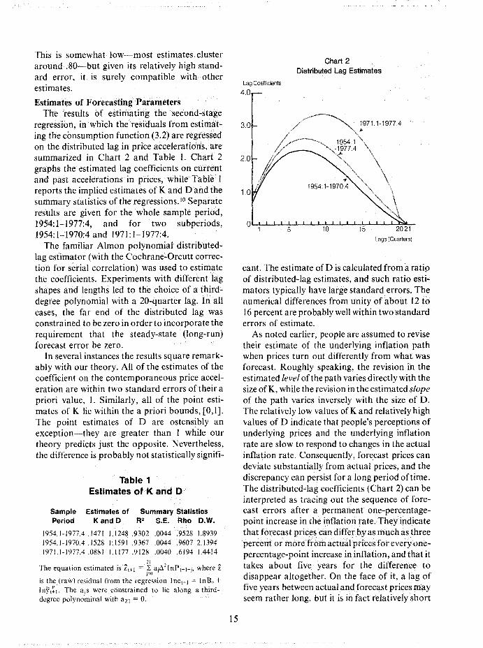
Chart 2Distributed Lag Estimates

cant. The estimate of D is calculated from a ratipof distributed-lag estimates, and such ratio esti-'mators typically have large standard errors. Thenumerical differences from unity of about 12 to16 percent are probably well within two standarderrors of estimate.

As noted earlier, people are assumed to revisetheir estimate of the underlying inflation pathwhen prices turn out differently from what wasforecast. Roughly speaking, the revision in theestimated level of the path varies directly with thesize of K, while the revision in the estimated slopeof the path varies inversely with the size of D.The relatively low values ofK and relatively highvalues of D indicate that people's perceptions ofunderlying prices and the underlying inflationrate are slow to respond to changes in the actualinflation rate. Consequently, forecast prices candeviate substantially from actual prices, and thediscrepancy can persist for a long period oftime.The. distributed-lag coefficients (Chart 2) can beinterpreted as tracing out the sequence offore­cast errors after a permanent one-percentage­point increase in the inflation rate. They indicatethat forecast prices can differby as much as threepercent or morefrom actualprices for every one­percentage-point increase in inflation, and that ittakes about five years for the difference todisappear altogether. On the face of it,a lag offive years between actual and forecast prices mayseem rather long, but it is in fact relatively short

This is somewhat low-most estimates clusteraround.80~but given its relatively high stand­ard error, it is surely compatible with otherestimates.

Estimates of Forecasting ParametersThe results· of estimating the second-stage

regression, in which the residuals from estirriat~

ing the consumption function (3.2) are regressedon the distributed lag in price accelerations,aresummarized in Chart 2 and Table 1. Chart 2graphs the estimated lag coefficients on currentand past accelerations in prices, while Tablelreports the implied estimates of K and D and thesummary statistics of the regressions. lo Separateresults are given for the whole sample period,1954: 1-1977:4, and for two subperiods,1954:1-1970:4 and 1971:1-1977:4.

The familiar Almon polynomial distributed­lag estimator (with the Cochrane~Orcutt correc­tion for serial correlation) was used to estimatethe coefficients. Experiments with different lagshapes and lengths led to the choice ofathird­degree polynomial with a 20~quarter lag. In allcases, the far end of the distributed lag wasconstrained to be zero in order to incorporate therequirement that the steady-state (long-run)forecast error be zero.

In several instances the results square remark­ably with our theory. All of the estimates of thecoefficient on the contemporaneous price accel­eration are within two standard errors of their apriori value, 1. Similarly, all of the point esti­mates of K lie within the a priori bounds, [0,1].The point estimates of D are ostensibly anexception-they are greater than 1 while ourtheory predicts just the opposite. Nevertheless,the difference is probably not statistically signifi-

Table 1Estimates of K and D

Sample Estimates of Summary StatisticsPeriod K and D R2 S.E. Rho D.W.

1954.1-1977.4 .1471 1.1248.9302 .0044 .9528 1.89391954.1·1970.4 .1528 1.1591 .9367 .0044 .9607 2.13941971.1-1977.4.0881 1.1177 .9128 .0040 .6194 1.4414

21

The equation estimatediszt+1 = ~ a jC121nPt+l_ j • where Zj::;:O

is the (raw) residual from the regression InCt+1 = InR. +Inytr l . The UjS were constrained to lie along a third­degree polynominal with aZI = O.

15

Lag Coefficients

4.0

3.0

2.0

1971.1-1977.4~

Lags (Quarters)

by comparison with typical results obtainedfrom studies of the relationship between pricesand interest rates. Some observers have rejectedthese long lags as being implausible, givellourknowledge of how prices are formed. I I However,once errors of measurement are allowed, theymay not be so implausible: where one is unsureabout the amount of information contained inprice movements, it is not irrational to ignorethem unless they continue for a long time.

The low values of K and high values of D alsosuggest that most of the uncertainty in forecast­ing prices stems from measurement error inprices, i.e., from the fact that a significant partofthe observed variation in prices represents ran­dom shocks which are unrelated to systematicinflation. The decline in the value of K for thelater subperiod suggests as well that prices havebecome more unpredictable since 1970. Thispoint has been made elsewhere on the basis ofdifferent evidence, 12 and agrees with one's casualimpression that the price level in the Seventieshas been subject to more frequent and severeshocks than was the case in prior decades.

Estimates of Underlying Inflation Rate_ Estimates of the underlying inflation rate,4>t+1 , along with the actual quarterly inflationrates, are shown in Chart 3. Clearly, the esti­mates of the underlying inflation rate have thesort of properties one would expect of such aseries: a much greater quarter-to-quarter stabili­ty than the actual inflation rate, and an ability totrack faithfully the longer-run movements in theactual inflation rate. However, the underlyinginflation rate can differ from the actual rate forsubstantial periods of time, reflecting the longadjustment lags.

It is also clear that successively higher levels ofinflation have become embedded in the economysince 1960. Thus the underlying inflation ratefluctuated around l.7 percent until the lateSixties, averaged about 4.8 percent from 1971 to1973, and in the current expansion has hoveredaround 7 percent. Apparently, neither the1969-70 nor the 1973-75 recession made a siz­able dent in the underlying rate; at most, theyseemed capable only of stabilizing the inflation

Chart 3

Actual and Underlying Inflation Rates

1962 1964 1966 1968

oHf-------,j----,j--

-1 =-~~~-":=~""":_:1954 1956 1958

3

2

4

6.

5

9

8

10

11

Annual Rate (%)

12

7

16

rate until some new disturbance carried it off to ahigher plateau.

There is no evidence that the 1971 priceandwage controls had any noticeable effect on peo­ple's perceptions about the underlying inflationrate. The decline in the underlying inflation rateafter the second quarter of J971 was negligiblecompared to the fall in the actual rate, and it didnot last as long. Some numbers make this pointmore forcefully. In the four quarters ending in1971:2, the inflation rate, measured by thegrowth in the GNP implicit price deflator, aver­aged 5.2 percent. In the four subsequent quar­ters, inflation declined by nearly 1Yz percentagepoints to 3.8 percent. By comparison, the under-

lying inflation rate was 4.8 percent in the firstperiod, and 4.9 percent in the second­effectively unchanged, in other words.

Much of the spectacular run-up in inflationrates in late 1973 and in 1974 appears to havebeen treated by economic participants as trans­itory, and thus was not viewed as symptomatic ofa deterioration in the underlying rate (thoughthat did happen). This perception was borne outby the subsequent sharp decline in inflation ratesafter 1974. By the same token, the underlyingrate did not follow the actual rate down as thelatter fell from its 1974 highs. Again, this percep­tion appears to have been borne out by thebounce-back in inflation rates after mid-1976.

IV. Summary and ConclusionsObviously, the estimates of the underlying Secondly, even if aggregate-demand growth

inflation rate calculated here should not be could be moderated, pressure for price and wageaccepted uncritically. Nevertheless, the congru- increases would continue to emanate from theence of our estimation results with the predic- cost side for a considerable time. The implicationtions of theory, and their conformance with of this for output and employment is not reassur-historical experience, are too striking to be ing. If pressures from inflationary expectationsignored. This congruence lends our estimates a do not abate after growth in aggregate demandhigh degree of plausibility. slows down, the difference presumably has to

Two points seem worth repeating because they come out of real income growth. This is essential-bear on the important question of what a suc- ly the modern explanation for the observedcessful assault on inflation is likely to cost in trade-off between unemployment and inflationterms of lost output and employment. First, the described by the Phillips Curve. This explana-ingrained rate of inflation currently perceived by tion of course stresses the temporary nature ofthe market is dismally high by historical the trade-off. Once expectations of inflationstandards-around 7 percent at an annual rate- have fully caught up with the actual rate, outputand has stubbornly remained at this level and employment are assumed to return to theirthroughout the current expansion. This persis- normal levels. But our finding about the lengthtence of a high perceived underlying inflation of the adjustment period-about five years-rate doubtless has given inflation an important suggests that temporary can still be a long time.momentum oUts own, because market partici- Hence, output and employment may have topants, in an effort to protect themselves against remain below normal levels for a fairly protract-future iI1flation, have built this perception into ed time if any significant progress is to be madetheir wage and price demands. against inflation.

FOOTNOTES

1. For some evidence that the market discounts spuri­ous evidence of inflation in the consumer price indexsee, E. Fama, "Interest Rates and Inflation: TheMessage in the Entrails,"American Economic Review,67 (June 1977), pp. 487-96.

2. Some controversy surrounds the proposition implic­it in (1.1) that consumption is strictly proportional topermanent income. This restriction was not imposed in

17

the estimation, but the empirical results were so con­sistent with it that I have written (1.1) in the traditionalform.

3. The variable u, which can be interpreted to be theratio of actual to planned consumption, has a lognor­mal distribution if we assume, in the usual way, that 1n uis normally distributed. Hence the assumption that themean of 1n u is zero corresponds to assuming that the

median ratio of actual to planned consumption is unity,and it is in this sense that actual and desired consump­tion are "on average" the same.

4. A good account of the theory involved can be foundin A. Bryson and Y. Ho, Applied Optimal Control (Wal­tham, Mass.: Blaisdell, 1969J

5. K has a steady-state solution for constant<t>.AI­though obviously we do not wantto assume the latter,we shall assume that the relative variation in <t> is sosmall that K is approximately constant. There .is ampleprecedent in the literature for doing· so, presumablybecause without such a simplification the forecastingproblem has no closed-form solution,

6. The expression for D is

D=

O*~ (1+<t>I) 2+ o~

where, as before, 0*2 measures the uncertainty inunderlying prices and o~ stands for the uncertaintyabout the underlying inflationary process. Clearly D isbounded from above by a number less than 1, while itcannot be less than zero.

7. To be totally consistent, we should add to consump­tion the imputed service flow from the existing stock ofconsumer durables. We did not do this simply becausequarterly estimates are not readily available; it is doubt­ful that the omission has any practical significance.

8. For a more thorough discussion of this point,see A.Alchian and B. Klein, "On a Correct Measure of Infla­tion," Journal of Money, Credit and Banking 5 (Febru­ary 1973, Part Ill, pp. 173-91.

9. For an up-to-date survey of evidence on the con­sumption function, see R. Ferber,"Consumer Econom-

ics: A Survey," Journal of Economic Literature 11(December 1973), esp. pp. 1307-08. Estimating (3.1) intwo stages does not appear to have affected the esti­mates except trivially. When (3.1 J is estimated in onestep, the estimate of the marginal propensity to con­sume is .78 rather than .75, while the estimated incomeelasticity is .98 rather than 1-differences which arewithout statistical or economic significance. Thedistributed-lag estimates are even less affected: theyare virtually indistinguishable from the estimatesgraphed in Chart 2.

10. The estimates of K and D are obtained by substitut­ing the estimated aj into the restrictions aj+l = (2(1-KJ +DK) aj - (1-KJ aj-l = 0 and solving for K and D. Thechoice of which aj to use is arbitrary: any four consecu­tive ones will do, and I chose a2 through a5. See G. Boxand G. Jenkins, Time Series Analysis (San Francisco:Holden Day, 1970), page 383.

11. See for example, T. Sargent, "Interest Rates andPrices in the Long Run," Journal of Money, Credit andBanking 5(February 1973, Part 11), pp. 384-449.

12. B. Klein, "Our New Monetary Standard: The Meas­urement and Effects of Price Uncertainty,1880-1973,"Economic Inquiry 13 (December 1975), pp. 462-84,argues that the shift from a monetary constitutionbased on the gold standard to a managed fiduciarystandard increased uncertainty about future prices. Heplaces the watershed in the mid-Sixties, at the latest.However, my experiments with different subperiodsproduced clear evidence for a break around 1970. Myconjecture is that it took the monetary laxity of the lateSixties to convince the public that monetary arrange­ments had fundamentally changed-a perception thatwas soon borne out by the collapse of the BrettonWoods System.

REFERENCES

Alchian, Armen and Klein, Benjamin. "On a CorrectMeasure of Inflation," Journal of Money, Credit andBanking 5 (February 1973, Part 1), pp, 173-91.

Box, George, and Jenkins, Gwilym. Time Series Analy­sis, San Francisco: Holden Day, 1970.

Bryson, Arthur, and Ho, Yu-Chi. Applied Optimal Con­trol, Waltham, Mass.: Blaisdell, 1969.

Darby, Michael. "The Allocation of Transitory IncomeAmong Consumer's Assets," American EconomicReview 62 (December 1972), pp. 928-41.

David, Paul, and Scadding, John.. "Private Savings:Ultrarationality, Aggregation and 'Denison's LaIN',"Journal of Political Economy 82 (March"Aprll1974), pp. 225-50.

de Leeuw, Frank. "A Model of Financial Behavior," in J.Duesenberry, G. Fromm, L. Klein and E. Kuh, eds.,The Brookings Quarterly Econometric Model of

18

the United States, Chicago: Rand McNally, 1965,Chapter 13.

Fama, Eugene. "Interest Rates and Inflation: TheMessage in the Entralls."American Economic Re­view 67 (June 1977), pp. 487-96.

Ferber, Robert. "Consumer Economics: A Survey,"Journal of Economic Literature 11 (December1973), pp. 1303-43.

Klein, Benjamin. "Our New Monetary Standard: TheMeasurement and Effects of Price Uncertainty,1880-1973," Economic Inquiry 13 (December1975), pp. 461-84.

Modigliani, Franco, and Sutch, Richard. "Innovations inInterest Rate Policy," American Economic Review65 (May 1966), pp. 178-97.

Sargent, Thomas. "Interest Rates and Prices in theLong Run," Journai of Money, Credit and Banking5 (February 1973, Part II), pp. 385-449.

Michael W. Keran*

Why has the international value of the dollardeclined over the past year and a half? There is apopular impression (sometimes reinforced by therhetoric of government officials) that the dollarhas been driven down by speculators who have avested interest in seeing an undervalued dollar.According to this view, the magnitude of thedecline is unrelated to economic fundamentalsand represents the irrational behavior of spec­ulators.

Most economists have difficulty with thisexplanation. A considerable body of evidenceshows that speculation tends to drive the value ofa currency towards the long-run equilibriumvalue; i.e., value determined by economic fun­damentals. Those who misjudge fundamentalsand attempt to drive the dollar away from itslong-run equilibrium value will tend to losemoney. On the average they will buy when themarket value is high and sell when the marketvalue is low. Those speculators who most clearlyperceive the underlying fundamentals and ac­cordingly take a position in the exchange marketwill, on average, make the most profits.

What this means is that stabilizing speculationwill tend to be profitable and destabilizing specu­lation to be unprofitable. 2 The self-selectionprocess of unsuccessful speculators leaving themarket to the successful speculators has impor­tant implications for the exchange markets. Inparticular, the observed value of the dollarwould not deviate significantly from the levelconsistent with economic fundamentals for morethan a short period of time.

Two types of economic factors affect the

* Senior Vice President and Director of Research,Federal Reserve Bank of San Francisco. Researchassistance for this article was provided by StephenZeldes.

19

exchange rate-real factors and monetary fac­tors. The real factors have to do with the relativeattractiveness of any two countries' goods, i.e.,how many bushels of U.S. wheat are exchangedfor one Japanese color T. V. set. This is called theterms of trade. The monetary factors have to dowith the purchasing power of a currency. Ifinflation reduces the domestic purchasing powerof the dollar, a parallel decline in the dollar'sforeign purchasing power will be achieved by anexchange-rate adjustment. This is called pur­chasing power parity.

The purpose of this article is to explain move­ments in the exchange value of the dollar againstthe currencies of seven other major countries(Canada, France, Germany, Japan, Italy, Switz­erland and the U,K,), during the period offlexible exchange rates running from roughly1974 or 1975 through March 1979. The analysisfocuses on whether monetary factors can explaina significant share of the movements of the dollaragainst these seven major currencies. Section Idiscusses the role of monetary factors in influen­cing prices in general. Section II discusses themonetary and real determinants of exchangerates, with the aid of a model which permits theempirical estimation of the monetary factorsaffecting the exchange rate. In Section III, com­parative monetary developments in the U.S. andother industrial countries are analyzed andshown to be in close alignment with observedmovements of exchange rates. Forillal statisticalanalyses confirm that a significant share of thevariation in exchange rates between the dollarand seven other currencies can be explained bymonetary factors. That section provides fore­casts of exchange rates based on actual monetarydevelopments in 1978 and forecasts of monetarydevelopments in 1979. Section IV gives a sum­mary and conclusion.

I. Money and PricesThe monetary source of exchange-rate

changes is based on two propositions:I) The exchange rate between two domestic

currencies will adjust to reflect changes in therelative domestic purchasing power of the cur­rencies (i.e., purchasing power parity); and

2) Domestic monetary developments are amajor determinant of domestic inflation rates,and thus the domestic purchasing power of agiven currency.

The second of these propositions is the mone­tary theory of inflation-too much money chas­ing too few goods. In its simplest form, thistheory can be stated as follows:

In the long run, the inflation rate (% D.P) isdetermined by the difference between the growthof the nominal money supply (% ~MS) and thereal money demand (% ~md). The nominalmoney supply is determined by the governmentthrough its monetary authority. The real de­mand for money is determined by the privatesector of the economy. The primary motivesbehind the demand for money are as a means ofpayment and as a store of value. The means-of­payment desire for money is dependent on thevolume of transactions, which in turn is relatedto the level of a country's real income. A rise inreal income leads to a rise in the real demand formoney.3

The store-of-value desire for money dependsupon the following factors:

I) The sophistication of the financial system,and the type and convenience of non-monetaryfinancial assets available to the public;

2) The real interest rate. The higher the realrate paid on monetary assets (e.g., time deposits),the higher the money demand; the higher the realrate paid on non-monetary assets, the lower thereal demand for money.

3) Inflation expectations. The higher the ex­pected inflation rate, the greater the expecteddecline in the value of monetary assets and thusthe lower the real demand for money.

There are a number of ways of translatingthese general principles into an empiricallytestable proposition. Perhaps one of the oldest

ways of stating this relation is via the familiarFisher Equation of Exchange.

This relationship states that, in long-run equil­ibrium, prices (P) will be equal to the ratio ofmoney supply to the long-run real demand for

(3)

(4)

(5)

(2)

M/P=T/V

md = T/V

MV= PT

P= M/md = M/(T/V) =ME

In long-run equilibrium, demand for realmoney balances must be equal to actual realbalances (M/ P). Thus, using equation (3), weidentify the long-run equilibrium value of M/ Pwith (md) and the long-run values of T and Vwith the determinants of money demand. Thus:

In this expression, where the bars refer to long­run equilibrium values, Trepresents the long-runmeans of payment function of money, while Vrepresents the long-run store of value function.

We next substitute this long-run behavioraldescription of money demand back into theequation of exchange to obtain:

The stock of money (M) times the velocity ofmoney (V) equals the physical volume oftransac­tions (T) times price level (P).

This is true by definition, analogous to thenational-income definition: National IncomeHousehold Consumption plus Business Invest­ment plus Government Spending. Just as thenational-income definition can be translated intoa statement of economic behavior by makingassumptions about consumption and investmentbehavior, so the Fisher equation ofexchange canbe by making assumptions about the factors thatdetermine the demand for money, i.e., velocityand transactions.

One can make equation 2 into a behavioralrelationship by introducing the demand for realmoney balances. If we rearrange terms in equa­tion 2, we obtain:

(I)% ~P = % ~MS - % ~md

20

money balances. This ratio is defined as excessmoney balances (ME). An expression similar toequation (1) can, of course, be obtained bytaking the time rate of change of all variables in(5) to obtain:

% ~P = %~M - % ~(T/V) = % ~ME (Sa)

This expression summarizes the main point ofthe monetary theory of inflation-that ultimate­ly inflation is determined by excess moneygrowth (%~ ME). This excess money supply isthe key element in the monetary factors whichdetermine the exchange rate.

II. Detennination of Exchange RatesThe exchange rate between the currencies of

any two countries will be determined by twofactors, one monetary and one "real." Theseseparate influences can be summarized in thefollowing way:

Where Ex is the exchange rate between the U.S.dollar and some foreign currency (t). Pus is thelong-run equilibrium price level in the U.S.; Pr isthe long-run equilibrium price level in the foreigncountry; t is the equilibrium terms of trade. Themonetary effects are measured by the relativeprice (Pr{Pus), while the real effects are mea­sured by the terms of trade (t).

I. Real effects: The terms of trade measure thevalue ofone country's goods in terms of the valueof another country's goods, e.g., how manybushels of U.S. wheat it takes to "purchase" oneJapanese T. V. set. A change in the terms of tradecould be caused by a change in technology, thediscovery of new sources of raw material, or asubstantial change in relative prices of importantcommodities, such as a rise in the price of oil.

2. Monetary effects: Exchange rates fluctuateto maintain equality between the domestic andforeign purchasing power of a currency, accord­ing to the theory of purchasing-power parity (orPPP). A rise in U.S. prices will reduce thedomestic purchasing power of the dollar. Thiswill increase the demand for lower-priced foreigngoods and assets, which will depreciate the dollarrelative to the foreign currency. The incentive toincrease demand for foreign goods will subsideonly when the dollar has depreciated by anamount equal to the decline in its domesticpurchasing power, assuming foreign-currencyprices are unchanged. Because monetary factorsdetermine the domestic purchasing power of a

Ex = (Pr / Pus) . t (6)

21

currency (for reasons already discussed), so theyalso influence the international exchange valueof that currency.

Purchasing-power parity can be explained in anumber of interrelated ways. Theoretically, themost general explanation is related to the neu­trality of money. If the money supply is doubled,all prices will double-or the purchasing powerof money will be reduced by half. For thisproposition to hold for all goods, both domesticand foreign, the exchange value of the domesticcurrency must fall by one-half relative to foreigncurrency (assuming there is no change in theexcess supply of money abroad). In this way, thedomestic and international purchasing power ofthe domestic currency are equal, and the neutral­ity of money is preserved. If the foreign moneysupply is doubled at the same time as the domes­tic money supply, the exchange rate will beunchanged, because foreign prices will go up asmuch as domestic prices.

The market mechanism by which the adjust­ment process operates is sometimes called thelaw of one price. This is based on the propositionthat the same goods will have the same price in allmarkets. For example, the dollar price of wheatin Kansas City will be the same as the yen price inTokyo, given the dollar/yen exchange rate. If theprice of wheat were higher in Tokyo than inKansas City by more than transportation, tariffsand other costs, then sufficient wheat will beshipped to Japan to drive its price toward equali­ty with the U.S. price.

Short vs. Long Run ConsiderationsIn Section I, we emphasized that the relation

between money and prices was a long-run prop­osition. Equilibrium in the market for goodstakes some time to achieve, because householdsmust change their consumption habits and firms

% ilEx = % il(MEr / MEus) + % ilt (9)

Log Ex = ao + al log (MEr / MEus) (8)

Taking the logs of both sides and making thesimplifying assumption that the terms of tradj::are constant, we can empirically estimate theequation as follows:

(7)Ex = (M& / MBus) . t

The changes in the exchange rate are equal to aconstant term (ao ') which measures the changesin the real factors, plus a coefficient (al') whichmeasures the impact on exchange rates of thechange in the ratio ofthe excess money growth inthe U.S. and in the foreign country. This ishypothesized to equal unity. The time lag inequations 8 and 10 reflects the length of timeneeded by market participants to recognize that

Assuming that the real factors which affectexchange rates-i.e., the terms of trade (%ilt)-change at a constant rate, we obtain theempirically testable equation:

measure of long-term PPP than are currentgoods prices. Second, because prices of tradedgoods increase with a decline in the exchangevalue of the dollar, and because traded goods area significant component of the general priceindex, the time lag between money and pricesmay be shortened when a country moves fromfixed to flexible exchange rates.

Where aa is a measure of an unchanged terms-of­trade effect on the exchange rate, and al is ameasure of the monetary influence on the ex­change rate. Its value is expected to be positiveand equal to one. Alternatively, we can expressequation 7 in terms of changes:

The ModelThis discussion can be formalized and an

equation specified for empirical testing. Giveninitial condition values for the exchange rate andexcess money, and substituting equation 5 intoequation 6, we get:

must change their production patterns. It iscostly for households to speculate on inflation bypurchasing goods in excess of consumptionneeds, because the cost of holding "inventories"is high. While anticipatory purchases in a periodof rising prices will occur, the amount is severelylimited. Thus goods prices will adjust only slowlyto a rise in excess money supply.

In contrast, the market for assets seems toadjust relatively quickly to changes in supply anddemand, because "inventory" adjustments inassets can be achieved at low cost. One canrearrange his portfolio of assets by "instanta­neous" buy-and-sell decisions at relatively lowtransactions cost, and generally zero carryingcost. In general, we assume that goods prices in"flow" markets take longer to adjust to shifts insupply and demand than assets prices in "stock"markets.

This distinction has important implicationswith respect to the monetary determinants ofexchange rates. The exchange rate-the interna­tional price of the dollar-can be affected byshifts in the international supply and demand fordollars, which in turn depend upon internationaltrade in goods, services, and financial assets.Trade in goods and services changes relativelyslowly in response to changes in income andprices, as is typical of all "flow" markets. Buttrade in financial assets can change quickly, as istypical of all "stock" markets.

The exchange rate, in the short run, thus isdetermined by the capital account of the balanceof payments. A change in the excess moneysupply (once recognized) could translate imme­diately into a change in the exchange rate. Themonetary effect on the exchange rate would bethe same in magnitude as that on the domesticinflation rate. The only difference would be interms of timing: the effect on the exchange ratewould occur quickly, while the effect on the priceof domestically produced goods would bedelayed.

This analysis has several important implica­tions. First, the exchange rate between the dollarand any foreign currency will measure the equi­librium purchasing power parity of the twocurrencies. If the exchange rate adjusts quicklyand prices adjust slowly to the same excessmoney supply, the exchange rate may be a better

22

the relative excess supplies of money hadchanged. This might well vary between coun­tries, depending upon the country's past mone­tary policy and inflation experience.4 Intro­ducing time lags into equations 8 and 10produces the basic estimating equations whichwill be considered in the next section.

nlog EXt = ao + raj log (MEr! MEus)t-n

(II)

n~log EXt = ao' + Iaj' ~log(MEriMEuS>t-n

(12)

nWhere I refers to the sum of months in whichchanges in excess money will have their completeeffect on the exchange rate.

UI. Testing the Monetary ApproachWe present evidence here to support the prop­

osition that monetary factors explain a signifi­cant share of the recent movements in the ex­change value of the dollar against seven othercurrencies. First, we present a summary of theapparent monetary-policy considerations whichshaped monetary developments in the 1975-78period. Then we show that the actual changes inthe excess money supply led to changes in pricesand. exchange rates in a way consistent witheconomic theory. Finally, we present formalstatistical tests of the relationship between mon­ey and exchange rates which confirm and quanti­fy the empirical relations.

Monetary Policy 1975-78In the summer of 1975, all eight countries in

this study faced a common set of economicproblems-two or more years of double-digitinflation and the recent emergence of a businessrecession which, for most countries, was theworst in the post-World War II period. Differentgovernments (and their monetary authorities)responded to these twin problems in differentways.

In the U.S., the primary goal apparently wasto deal with the historically high unemploymentrate by following a monetary policy which per­mitted a substantial acceleration in aggregatedemand from 1975 through 1978. Other coun­tries such as Germany, Japan and Switzerland,responding to the historically high inflation rate,apparently followed a monetary policy whichpermitted only a moderate acceleration in aggre­gate demand.

As a result of this divergence in monetarypolicies, short-run rates of real growth alsodiverged. The U.S. grew at a rate from 1975 to

23

1978 which was above its historical average, butthe reverse was true for Germany, Japan andSwitzerland. Over the longer run, these divergentmonetary policies led to divergent inflation rates.From 1976 to 1978 the inflation rate in the U.S.accelerated, while the inflation rates in Germany,Japan and Switzerland decelerated. Finally, thepolicy divergence between the U.S. and Ger­many, Japan and Switzerland led to a decline inthe exchange value of the dollar with regard tothe Deutschemark, yen and Swiss franc.

Marshalling the EvidenceIn broad outline, we assert that divergent

monetary policies have been the key factorbehind the divergent economic developmentsand exchange-rate movements of the past severalyears. The evidence in support of this scenario isprovided in Charts I and 2.5 Chart I shows thatfrom 1975 to 1978, the money supply in the U.S.grew at about the same rate as in Switzerland,and more slowly than in Germany and Japan.However, as discussed in the theoretical section,the relevant measure is not the growth in thenominal money supply, but rather the growth inthe excess money supply, which is nominalmoney less real money demand, as is shown inChart 2.

In estimating real money demand, the meansof payment (i.e., transactions) motive was mea­sured by the trend in industrial production, andthe store of value motive for holding money wasmeasured by the trend in velocity. Sixty-monthtrends of these factors were utilized, to reflecttheassumption that reversible cyclical shifts in thecomponents of real money demand would haveno effect on the long-term equilibrium price level

Chart 1Nominal Money Supply

1975=100

(P), and thus no effect on the exchange rate.6 Calculated on that basis, excess money growth in the U.S. was higher in the 1975-78 period than in Germany, Japan and Switzerland (Chart 2).

Domestic Results. The relationship between excess money growth and real output growth is a short-run phenomenon. Thus, we would expect that those countries with the highest excess money growth would, in the short run, exhibit the most rapid growth in real output. The results in Table 1 and Chart 2 confirm that result. The U.S., where growth in excess money has been fastest among the four countries since 1975, has also had the fastest rate of real growth. Germany, with the slowest growth of excess money, has had the slowest real growth, and Japan and Switzer­land have fallen in between.7

The relationship between excess money growth and prices is a long-run phenomenon. Thus, excess money-growth patterns would not necessarily be completely reflected in the ob­served price patterns for consumer and whole­sale prices to date. (Tables 2 and 3). For all four countries and for both price indexes, the inflation rate has dropped substantially since 1974. The U.S. and Japan recorded almost the same average consumer-price inflation rate in

the last four years (close to 7 percent)— substantially higher than that observed in Germany (4 percent) and Switzerland (2 per­cent). In the period 1977.3-1978.3, however, Japan’s inflation rate had decelerated to 4 percent, and the German and Swiss rates have also decelerated, while the U.S. rate has accelerated to almost 8 percent. As a result, the spread in the consumer inflation rates between the U.S. and the other three countries has widened recently in line with the differences in their excess money growth.

The same basic pattern emerges with respect to wholesale prices, but with an even wider spread since 1977.3. For one reason, there is a larger weight of traded goods in the wholesale index than in the consumer index. Thus, changes in the exchange rate which directly affect inter­nationally-traded goods prices will have a larger and more immediate impact on the WPI than on the CPI. This may be the genesis of the vicious vs. virtuous cycle argument. Countries whose mone­tary policies tend to decelerate inflation experi­ence an immediate favorable impact on the exchange rate which reduces the inflation rate promptly; while countries whose monetary poli­cies tend to accelerate inflation suffer an immedi­ate unfavorable effect on the exchange rate which promptly adds to domestic inflation. This vicious/ virtuous cycle should be considered a

Chart 2

24

reflection of the timing of the monetary impacton prices, rather than as a new destabilizingphenomenon. This subject is discussed further inSection IV.

Exchange Rate Results. These domestic re­sults are broadly consistent with the assumptionsof relatively easy monetary policy in the U.S. andrelatively tight monetary policies in Germany,Japan and Switzerland. To measure the impactof these assumed divergent policies on exchangerates, we have computed a "monetary index"­the ratio of the excess money supply in the U.S.to the excess supply in each of the other coun­tries. Each monetary index is scaled to thecorresponding exchange rate by the coefficientsestimated in the equation in the appendix of thisarticle. As indicated in Chart 3, this monetaryindex shows a high degree of correspondencewith the movement in the bilateral exchange rate

Table 1Industrial Production

(Annual Rate ,of Change)

1963-73 1973-75 1975.1-1978.3

Germany 5.1 -4.3 2.1Japan 12.3 -7.5 6.7Switzerland 4.6 -6.7 3.0United States 5.4 -4.7 7.8

Table 2Consumer Price Index

(Annual Rate of Change)

1973.4- 1974.4- 1977.3-1974.4 1978.3 1978.3

Germany 6.5 4.0 2.5Japan 24.4 7.3 4.0Switzerland 8.7 2.0 1.0United States 12.1 6.8 7.9

Table 3Wholesale Price Index

(Annual Rate of Change)

1973.4- 1974.4- 1977.3-

1974.4 1978.3 1978.3

Germany 13.4 2.5 1.2

Japan 23.5 0.9 -3.3

Switzerland 12.7 -2.4 -4.0

United States 22.2 5.6 8.3

25

between the dollar and each of these three cur­rencies. In each case, the monetary index de­clined in 1974, rose slightly in 1975 and early1976, and then declined substantially throughthe end of 1978. This movement in the monetaryindex is paralleled by a similar movement in theexchange rate. The major decline in the exchangevalue of the dollar was accompanied by a majorexpansion in the excess money supply in the U.S.relative to the other three countries.

In general, adjustments of exchange rates tochanges in the monetary index appeared to occurquickly-within a quarter of a year or so. Andthe magnitudes of these exchange-rate adjust­ments were approximately the same across coun­tries for any given change in the monetary index.This observation is consistent with the hypothe­sis developed in Section II, that the exchangerate in the short run is dominated by the capitalaccount of the balance of payments, and that itthus responds quickly-in a way analogous toany domestic-asset market response to changesin supply and demand.

The same broad relationship of monetaryindexes and bilateral exchange rates holds forCanada, France, Italy and the U.K.. The resultsfor France and Italy are detailed in Chart 4. Withthese four countries, however, the lags betweenchanges in the monetary index and the exchangerate seem to be longer and the degree of relation­ship weaker, than in the case with Germany,Japan and Switzerland for a number of reasons.First, Germany and Japan are leading economicpowers in their own right, so that their currenciesare potential replacements for the dollar as aninternational currency. Also, the Swiss franc hasa unique role as an international store of value,and the Swiss monetary authorities havefollowed a more restrictive monetary policy thanmost of the countries studied.

Second, excess money-supply growth has beeneven greater in Canada, Italy and the U.K. thanin the U.S. over the 1974-78 period. (Frenchgrowth has been slightly less expansionary). As aconsequence, the dollar generally strengthenedagainst these currencies before weakening in thesecond half of 1977. The recent weakness of thedollar may in part reflect a spill-over of the ap­preciation of the Swiss franc and especially theD.M. onto other European currencies. This

would occur among the European currencies if acommon set of "real" exchange rate influencesoperated. (The dollar's relative strength againstthe Canadian dollar supports this conjecture.)

Third, in the case of the U.K., a special realfactor may explain the relative weakness ofthedollar. That factor is the recent favorable effectof North Sea oil on the British balance of pay­ments.

The evidence presented above tends to supporta monetary interpretation of much of the recentmovements in the exchange value of the dollar,

especially against the D.M., the yen and theSwiss franc-and substantially with respect tothe Canadian dollar, the Italian lira, the Frenchfranc and the British pound. The next step is topresent evidence in a more formal econometricsetting. This will help show whether the relation­ship between the monetary index and the ex­change rate is significant and stable within arigorous statistical testing procedure. Thosereaders who are not interested in this necessarilytechnical discussion should proceed to the sec­tion on forecasting exchange rates on page 30.

Chart 3Money' and Exchange Rates

Switzerland

3.4 108Francs/$ Monetary Index

Germany

1063.2Japan

106Monetary IndexDM/$

2.8

340Yen/$

30 1042.7 104

r'Monetary Index

\\320

2.6 102 102 2.8 ", \ 102

. -.:/"\ -.\) i\»-300

J1002.5 100 ff'\ 2.6 \}\ 100

\280

, \\ "

98 '~ 98 2.4 982.4260 \-0lil( \96 96 2.2 962.3

\\240 ~

2.2 94 220 2.0 94

\\92 200 182.1

\~

\, 18090 1.6 902.0 90

160....1978 88 1978 881.9 1974 1976 1978 88 1974 1976 1.4 1974 1976

'Monetary Index=Ratio of excess money supplyih foreighcountry to excess U.S. money supply.

26

Formal Statistical TestsThe exchange rates to be tested are the bilater"

al rates between the U.S. dollar and the sevenforeign currencies discussed above. The coun­tries were selected on the basis of data availabili­tyand importance in international trade andfinance.· All regressions were estimated withordinary least~squares (OLS) using a third­degree (or less) polynomial distributed lag(PDL). The equations were estimated with twoalternative measures of money published inInternational Financial Statistics-money, and

money plus quasi-money. The formeris thenarrow definition of money including currencyand demand deposits. This primarily statisfiesthe means-of-payment motive for holdingmo­ney. The latter is the broader definition whichincludes currency, demand deposits and quasi­monetary· deposits of commercial banks. Thismeasure includes a substantialstore-of-valuemotive for holding money.

While statistically significant results were ob­tained with both definitions of money, thebroader measure gave results which weregener-

Chart 4Money' and Exchange Rates

Italy

104

France

Monetary Index 106

3.9

3.8L19':'::7:-:4..L--L179:::-76~-.11':":9:-=7-:o'8 92

52Francs/$

5.1 i\5.0 /4.9

!4.8

4.6 .)4.5

4.4

\4.3

4.2

V4.1

4.0

95

90

110

105

100

130

120

125

135

1978 85

Monetary IndexII

I1.­iLJ/

650

700

800

750

900

850

950

1000 Lira/$

'Monetary Index=Ratio of excess money supply in foreigncountry to excess U.S. money supply.

27

ally superior. Given the dollar's role as both aninternational means of payment and store ofvalue, the superiority of the broader measure ofmoney is not surprising.

The equations for the seven bilateral exchangerates were estimated monthly from January 1974(or January 1975) to December 1977 in both leveland rate-of-change form, i.e., matching equa­tions II and 12. The level results are presented inthe appendix, and the rate-of-change (difference)results are presented in Table 4. The percent ofvariation explained (R2) is much higher in thelevel form than in the difference form, becausethe unsystematic variance is necessarily greaterin the latter. However, a better measure ofgoodness of fit is provided by the standard error,which measures the percentage error in explain­ing the exchange rate. The standard errors areabout the same for both forms of estimation.s

The major conceptual difference between thelevel and difference form is the implicit treatmentof real factors which affect the exchange rate. Inboth forms, the real factor is captured by the

constant term. In the level equation, we assumethat the real factors are unchanged over time, butin the difference equation, we assume that theychange at a constant rate over time. However, asthe constant term is both large and statisticallysignificant only for Italy in the difference form,there is only weak general evidence for a strongreal factor affecting the exchange rate.9 Thissuggests that either form of the equation wouldrepresent the underlying structure without majorsystematic bias. The remainder of the discussionwill be in terms of the rate-of-change equationsexcept where otherwise stated.

The monetary effect is measured by the sumcoefficient value (Ial')' It is a sum because itmeasures the combined effect of the current andlagged values of the monetary influence on theexchange rate. The coefficient values are statisti­cally significant in all cases. The lags between themonetary influence and the exchange rate mea­sure the total number of months needed for themonetary effect to operate. The lag periods wereselected on the basis of the minimum standard

Table 4Monetary Factors and Exchange Rates: Difference Form

nLllog EXt == a,,' + Ial' Lllog(MEr/ MEus)t-n

Estimation Degrees of Corrected

Country Period lags Freedom ao ~a l' R' S.E. RHO D.W.

Canada* 1974.01-1977.12 6-18 44 -.003506 1.076 .096 .0097 1.83

(-1.21) (2.16)

France 1975.01-1977.12 12 32 -.000053 1.761 .168 .0168 1.70

(-.17) ( 1.95)

Germany 1975.01-1977.12 9 32 -.000023 2.565 .137 .0177 1.45

(.07) (2.69)

Italy 1974.01-1977.12 9 44 ".03392 5.487 .332 .0193 .42 1.85

(-1.80) (2.27) (3.17)

Japan 1975.01-1977.12 6 32 -.004021 2.887 .205 .0132 1.73

(-1.75) (3.17)

Switzer-

land 1974.01-1977.12 2 45 -.002440 2.649 .135 .0227 1.54

(-.62) (2.96)

U.K.** 1975.01-1977.12 15 32 -.015769 3.060 .352 .0170 .44 1.61

(-1.29) (2.01) (2.90)

t -statistics in parentheses

* Includes only lags t-6 to t-18

** Uses log of deviation of Ml UK from trend

M 1 US

28

Forecast

Chart 5 (cont.)

1975 1976 1977 1978 1979

Estimation Period

In the theoretical discussion (Section II), wehypothesized that the expected value of themonetary influence on exchange rates would bepositive and equal in value to 1.0. This resultsfrom the method of calculating the monetaryinfluence-the ratio of excess money in the U.S.to excess money in each of the other countries.Excess money is, in turn, defined as the differ­ence between the change in nominal moneysupply and the change in real money demand. Ifmoney is homogeneous of the degree one inprices, i.e., if neutrality conditions hold, a perma­nent I-percent increase in excess money will leadto a I-percent increase in the long-run equilibri­um price level and, thus, to a I-percent decreasein the exchange value of the dollar, assuming nochange in excess money in other countries.

The estimated coefficient values are positivefor all of the countries considered in this study.However, only in the case of Canada and Franceare the coefficient values close to one. In the caseof Germany, Japan, Switzerland and the U.K.,the coefficient values fall within a narrow rangeof 2.5 to 3.1. Italy, on the other hand, fallssignificantly outside the range, with a coefficientvalue of 5.5. 10

One factor which can explain the divergencebetween the expected theoretical value and theactual measured value of the monetary influence

Francs/$

3.40

320

300

2.80

260

2.40

220

200

180

1.60

1.401974

29

Dynamic Forecast

Chart 5Exchange Rate Estimates

Estimation Period

error of estimate. In general, the lags variedsUbstantially between countries. They were theshortest for Switzerland (2 months), and Japan(6 months)-the countries with the shortest lagsbetween the monetary index and the exchangerate (Chart 3). The lags were longest for Canada(18 months), the U.K. (15 months), France (12months), and Italy (9 months). Germanyprovided the only exception to the generalparallelism of the formal statistical results andthe informal results in Charts 3 and 4, with itsrelatively long (9 months) lag compared to thoseof Japan and Switzerland.

Yen/$

320 Estimation Period Dynamic Forecast

300

280

260

240

220

200

180

1601975 1976 1977 1978 1979

DM/$

2.70

Table 5Forecasts of Money Growth Rates for 1979

The forecasts of the DM/ $ and ¥ / $ exchangerates were quite close to the actual decline invalue through March 1979. In the case of theSwiss franc (SF/$) rate, the forecast was rea­sonably accurate through mid-1978 and picked

1) An estimation period (1974-1977 forSwitzerland, and 1975-77 for Germany andJapan) where the fitted values of the exchangerate (Chart 5) are compared with the actualvalues of the exchange rate. For all threecountries, the equations accurately tracked themonthly movement in the exchange rate. 12

2) A forecast period (January 1978 to Decem­ber 1979), with actual money-supply growthused through November or December 1978, andwith money assumed to grow thereafter at thesame rate as it had grown over the previous 12months (Table 5).

To demonstrate the effects of U.S. monetarypolicy on exchange rates, two different sets offorecasts were performed. The first assumes U.S.money growth over 1979 to be equal to the actualrate of growth over 1978: 8.75 percent. Thesecond set of forecasts assumes a lower money­growth rate of 6.5 percent. These two forecastsare indicated by the two dotted lines in Chart5. No adjustment is made for past forecasterrors (i.e., the simulations are dynamic), so thatthe errors cumulate from the initial conditionmonth (December 1977) to the month beingforecast. As Chart 5 indicates, the forecastmoney-based exchange rate tracks the actualexchange rate with reasonable accuracy. Thefollowing table shows the actual and forecastchange in the exchange rate from December 1977to March 1979.

Percent16.011.010.022.513.09.0

15.08.75/6.5

CanadaFranceGermanyItalyJapanSwitzerlandU.K.13U.S.

Forecasting the Exchange RateThe results presented above, although tenta­

tive, provide a reasonable basis for making shortterm forecasts of exchange rates. Such forecastswould be useful because our equations· Wereestimated with data only through December1977 (Table 4), while some of the largest declinesin the dollar's value occurred in 1978 and wereonly partially reversed by the dramatic dollar­rescue operations announced on November I,1978. We can estimate the degree of monetaryinfluence on the exchange rate in 1978 by con­ducting dynamic simulations of our equations.

The results are presented for two time periods:

is measurement error with respect to the public'sreal demand for money. Errors of this type canoccur when there is a permanent shift in thedemand for money which is not captured by the60-month trend procedure. As discussed in Sec­tion I, inflation can have an importanteffectonreal demand for money. In countries which havebeen more successful than the U.S. in reducinginflation (such as Germany, Japan and Switzer­land) the real demand for money may be higherthan our measured demand for money.. Con­versely, in countries which have been less suc­cessful than the U.S. in reducing inflation (suchas Italy and the U.K.), the real demand for moneymay be less than measured demand. Assumingthat the real demand for money is accuratelymeasured in the U.S., the errors. in the othercountries could bias the monetary index. In allcases the bias would tend to make the observedindex move in a narrower range than the truemonetary index, with a smaller decline forthosecountries with a lower inflation rate than theU.S., and a smaller increase for those countrieswith a less successful recOfd than the U.S. incontrolling inflation. In each case, the measuredmonetary index would have a greater coefficientvalue than would the true monetary index. Thisanalysis is broadly consistent with the observedcoefficient values. Those countries with coeffi­cient values close to one (Canada and France)experienced roughly the same amount of infla­tion as the U.S., while those countries withcoefficient values substantially greater than onerecorded inflation rates which were significantlyabove or below the U.S. inflation rate. II

30

Table 6Exchange Rate Changes

(December 1977-March 1979)

the turnaround in late 1978, but it erred inforecasting the level of the exchange rate. Thereason behind this forecast error waS the sharpacceleration in Swiss money growth in the sec­ond half of 1978, which seems to have beenignored by the market until now. The modelpresented here suggests that if the money supply

Germany (DMI $)Japan (¥ 1$)

Switzerland (SF1$)

Actual(Percent)

-13.6-14.6-19.1

Forecast(Percent)

-14.0-12.0-8.6

Error(Percent)

.4- 2.6-10.5

grows at the rates indicated in Table 5, thenbetween March and December 1979 the dollarwill appreciate against the Swiss franc, be stableagainst the Japanese yen, and decline slightlyagainst the German D.M.

Very good results were obtained when thesame forecast experiment was conducted withrespect to the dollar and the French franc. InFrance's case, the error was only .6 percent overthe forecast period. However, the forecast errorswere in excess of 10 percent for Canada, Italy,and the U.K. In two cases (Italy and the U.K.),the actual dollar value was below the forecastvalue, while in one case (Canada), it was abovethe forecast value. In all three cases, significantnon-monetary factors apparently influencedthese exchange rates.

IV. Conclusion and ImplicationsThe major conclusion of this article is that an

important share of the exchange-rate move­ments of the dollar against key foreign currenciescan be explained by monetary factors, ratherthan by speculation or changes in such realfactors as the terms of trade. In addition, thestudy suggests two major implications:

I) Foreign-exchange markets adjust muchmore quickly than domestic commodity marketsto changes in domestic monetary conditions.

2) The emergence of flexible exchange ratescan shorten the lag between money and prices.

One of the most generally accepted proposi­tions in economics is that money affects goodsmarkets and, therefore, the inflation rate with arelatively long lag. On the other hand, it affectsasset markets and, therefore, interest rates witha relatively short lag. The reason for the differ­ence in response is that costs of adjustment aremuch higher in goods markets than in assetmarkets. It is difficult for a household to specu­late on a rise in the price of bread by buying morebread than it can currently consume. The storagecosts are high, and the depreciation on the valueof the good is substantial. As a result, householdexpectations of higher prices, even when stronglyheld, will not necessarily be translated immedi­ately into higher actual prices. Now consider thecase of an asset market, such as that for Treasurybills. If the price of T-bills is expected to rise in

31

the future, it will be instantaneously translatedinto a higher price of Treasury bills today. Forone reason, the transactions cost involved inshifting from one type of asset to another isrelatively low, and for another, the storage costsfor holding Treasury bills are virtually nil. Thus,we can expect nearly instantaneous adjustmentin asset markets to shifts in underlying supplyand demand.

This article extends asset-market analysis tothe exchange rate. We assert that the exchangerate is, in the short run, determined by the samefactors which determine the price of any asset.Thus, a monetary disturbance can be translatedrelatively quickly into a change in the exchangerate, even though the change in the underlyinginflation rate may be delayed. This suggests thatthe short-run deviation of the exchange ratefrom purchasing power parity may be substan­tial, even when the underlying cause of theexchange-rate change is a monetary rather than areal disturbance. Supporting evidence is pro­vided by the relatively short lags observed in themonetary index-the relation between U.S. andforeign excess money-supply growth rates -,- andin the resulting changes in the bilateral exchangerates of the dollar against foreign currencies. Fulllag adjustments for some countries were as shortas two to three months, and. were never longerthan eighteen months. The average lags were

shorter still. On the other hand, most empiricalevidence relating money to inflationsuggests anaverage lag of about two years, and full-effectlags of three to four years.

A second implication of this study concernsthe shortened link betweenmoney and prices as aresult of the introduction of flexible exchangerates. A rise in excess money supply in the U.S.would, with a relatively short lag, lead to adecline in the exchange value of the dollaragainst its major trading partners. For reasonsdiscussed above, this would tend to raise theprice not only of imported goods, but of allinternationally-traded goods, in dollar terms.American exporters would not sell in the U.S.market for a lower price than they could get forthe same product in a foreign market, standard­izing for transportation costs.· The rise intradeable-goods prices would increase the aver­age inflation rate in the U.S. by an amount equalto the weight of tradeable goods in overall priceindexes. The weights would vary •betweenindexes-high for the wholesale-price index(which includes only goods), but lower for theconsumer-price index (which includes services)and for the GNP price deflator (which incfudes

the cost of government).Direct evidence of a shortening of the lag

between money and prices would have to comefrom econometric tests of the lag structure. It isdifficult to acquire such evidence because oftherelatively short period in which flexible exchangerates have operated. However, a certain amountof indirect evidence supports this proposition. Tothe extent that inflation operates through theexchange rate rather than through standarddomestic markets, the price of goods (which areinternationally traded) may rise relative to theprice of services (which are not generally tradedinternationally) in the short run. This reversesthe traditional ordering of the effects of moneyon prices. Generally, wholesale-price indexestend to exhibit a lower average inflation ratethan consumer-price indexes, as a reflection ofthe higher productivity of goods industries thanservices industries. However, since the March1973 introduction of flexible exchange rates, therate of inflation in the goods-dominated (whole­sale) index has been higher than the rate ofinflation in the services-denominated (consum­er) index. This is consistent with an internationalexplanation of much of the recent inflation.

AppendixMonetary Factors and Exchange Rates: level Form

nlog EXt = aa + kal log (MEr/MEus)t-n

Estimation Degrees of CorrectedCountry Period lags Freedom ao la1 R2 S.E. RHO D.W.

Canada* 1974.01-1977.12 6-12 44 -.076 .826 .935 .0095 .93 1.82(-1.67) (3.00) (17.59)

France 1975.01-1977.12 12 32 1.297 2.682 .962 .0132 .58 I.71(49.40) (9.82) (4.28)

Germany 1975.01-1977.12 6 32 1.131 2.018 .892 .0168 .77 1.49(22.73) (5.17) (7.22)

Italy 1974.01-1977.12 3 44 6.611 1.163 .976 .0223 .92 .95(147.98) (3.81) (15.74)

Japan 1975.01-1977.12 2 33 6.450 2.138 .941 .0145 .95 1.48(21.43) (3.04) (18.99)

Switzer-land 1974.01-1977.12 1.097 2.701 .945 .0222 .90 1.56

(15.97) (3.33) (14.07)U.K.** 1974.01-1977.12 12 44 -.687 1.148 .980 .0193 .92 1.04

(-17.30) (4.33) (15.78)t-statistics in parentheses* Includes only lags t-6 to t-12

** Uses log of deviation of MI UK from trendMI US

32

FOOTNOTES

1. The intellectual foundation behind this article is themonetary theory of the balance of payments. One Of theoriginal papers by Harry Johnson was published in1972 in the Journal of Financial and Quantitative Analy­sis. A surveyor recent works is presented in J.A.Frenkel and H.G. Johnson (EdsJ The Monetary Ap­proach to the Balance of Payments, 1976. Importantrecent contributions havebeen made by R. Dornbusch,forexample, "The Theory of Flexible Exchange .RateRegimes and Macroeconomic Policy," ScandinavianJournal of Economics (1977>'

2. There may be short-run situations when destabiliz­ing speculation is also profitable. This occurs when the"greater.fool" theory operates. An intelligent speculatormay believe that a currency is undervalued and still sellit because he perceives that other speculators believe itis still overvalued. One can make money in the short runby speculating about the actions of other speculatorsrather than about the economic fundamentals whichdetermine acurrency's long-run value. But this "greaterfool" approach can be profitable only for a limitedperiod of time.

3. Other important factors which influence the demandfor money as a means of payment are various institu­tional arrangements, such as the frequency with whichwages and salaries are paid. However, these factors willchange only slowly over time, and are not usually animportant source of a change in the demand for money.

4. Government intervention can also affect the ex­change rate, but we ignore these effects for severalreasons. Government intervention can fall under threeheadings: 1) actions to counter disorderly markets; 2)central-bank purchases and sales of foreign exchangefor own account; and 3) Treasury purchases or sales offoreign exchange through sale or redemption of debtdenominated in foreign-currency values. The first typeof intervention (countering disorderly markets) is bydefinition transitory and reversible. Thus it has nopermanent effect on the exchange rate, the balancesheet of the central bank, or the position of the Treas­ury. The second type of intervention affects the balancesheet of the central bank. Sustained intervention in theforeign-exchange market will either increase or dec­rease central-bank holdings of foreign assets, and thuschange the domestic money supply. This type of inter­vention is considered directly by the way the equation isestimated-through the excess money supply. Thethird type of intervention (sale of foreign-denominatedgovernment securities) affects the composition but notthe level of Government debt. Its effect on exchangerates is not captured by our empirical estimation proce­dures. However, this type of intervention is insignificantbecause of the recency and small scale of such opera­tions. The U.S. Treasury issued its first OM security inJanuary 1979 and its first Swiss franc security in Febru­ary 1979. The total amount authorized by the Treasuryis $10 billion, and the amount actually sold is $3 billion.

5. This broad definition of money includes currency,transactions deposits and quasi-money deposits ofcommercial banks. A fuller discussion of the monetarymeasures is given in the following section on statisticaltests.

33

6. More explicitly, log ME=log (M/\'f/iiJ), where f is thetrend level in industrial production, and ii is the trendlevel in velocity. Velocity equals industrial productiondivided by the real money stock. Real money is thenominal money stock (money plus quasi-money) de­flated by the wholesale-price index. The trend levelestimates are calculated recurSively by multiplyinglast period's trend level estimate by the rate of growth ofthe actual variable over the past 60 months. F6rexam­pie:

Veo = VeoRt = ( Vt - Vt-eo ) /60

Vt-eoVi = Vi-1 x (1 + Rt) For all t >60

This procedure was followed for all countries with theexception of the U.K., for which there was no monthlydata for quasi-money, and for which there was insuffi­cient monthly money data to calculate the trends. In theU.K. case, money alone was used, instead of moneyplus quasi-money, and the trend in real money demandwas estimated by extrapolating the average 1963-1973nominal money growth rates in the U.K. and the U.S.7. Other factors which could have explained thesedifferential growth rates, such as the size of the previ­ous business-cycle downturn or the trend growth in theeconomy, do not appear to have been significant. TheU.S. growth rate in the last three and a half years-7.8percent-was significantly above its 1963-73 trendgrowth of 5.4 percent. On the other hand, Germany's,Japan's and Switzerland's recent growth rates weresignificantly below their trend growth rates in thedecade ending in 1973. The size of the previousbusiness-cycle downturn also does not explain therecent strength in the U.S. growth rate. Both Switzer­land and Japan had a more severe downturn in theireconomy in the 1973-75 period than the U.S., whileGermany had a downturn equal tothat of the U.S. Thus,it appears that differences in monetary stimulation havebeen a key factor in differences of real growth rates ofthese four countries in the most recent business-cycleexpansion. The movement in the unemployment ratewas consistent with the pattern of growth rates inindustrial production. In the U.S., unemployment de­clined significantly by 1978 from its 1975 peak rate. InGermany, Japan and Switzerland, however, unemploy­ment rates were equal to or above 1975 rates. Thissuggests that real growth in those three countries hadbeen insufficient to absorb the natural growth in theirlabor force and productivity, and thus suggests thattheir growth had been below potential.

8. All of the level equations were estimated with Coch­rane/Orcutt adjustment for the first-order serial corre­lation of the error term.

9. In the case of Japan, the constant term is statisticallysignificant but quantitatively small. In the case of theU.K., the constant term is quantitatively large, but notsignificant statistically.

10. Italy is the only country in which the constant termhas a large and statistically significant value. Thissuggests that there were important real factors opera­ting on the Italian exchange rate as well as the moneyfactors modeled in the equation.

11. A related source of measurement error is associa~

ted with market expectations. Market participants mayview current nominal money growth as aprecursoroffuture growth in the nominal money supply. Theseexpectations could affect the exchange rate. ForexaTTl­pie, when market participants observe the steady decet.­eration over the last four years in Switzerland's nominalmoney growth, they might reasonably. expect. thatpattern to continue and, thus,. would forecast alowerlong-run equilibrium price and lower exchange value ofthe dollar relative to the Swiss franc than is implicitinthe actual trend of nominal money growth. Theseexpectational influences could bias the coefficientvalues either above or below one~above one if themarket extrapolated current monetary developments,and below one if the market expected the monetaryauthorities to revert to some trend value in the face of anobserved deviation in money.

34

To the extent that expectations have been importantin affecting coefficient values, these values may remainunstable over long periods of time. Indeed, if all mone­tary authorities followed constant money-growth rules,this expectation factor would no longer influence mar­ket participants and the coefficient values would movetoward unity.

12. The equations in Table 1 were estimated in differ­ence form, while the charts were displayed in level formfor convenience in interpretation. This transformationwas achieved by conducting a static simulation of theequations over the estimation period.

13. See footnote 6 for an explanation of why the narrow­er aggregate (money) is used for the UK, as opposed tothe broader aggregate (money plus quasi-money)which is used for the other countries. The correspond­ing growth rate for US money is 6 percent.

Michael Bazdarich*Over the last eighteen months, a number of

explanations have emerged for the dollar's de­cline in the foreign-exchange markets. One par­ticularly prominent theory attributes thedollar'sweakness largely to the relatively rapid growth ofthe American economy. The analysts proposingthis theory argue that fast economic growth in acountry causes an acceleration in its imports andtherefore a deterioration in its trade balance,ultimately leading to a depreciation of the do­mesticcurrency.

This paper questions the validity of that ap­proach. It argues instead that true economicgrowth, as evidenced by rapid growth in produc­tive capacity, or potential GNP, typicallystrengthens the domestic currency. Growth ofthis type implies improving supply and wealthconditions which can more than offset the effectsof rising demand on the trade balance. Sharpcyclical increases in GNP, on the other hand, canweaken the domestic currency. These move­ments typically involve an increase in demandwith no change in productive capacity, and so donot generate any offsetting effects to the rise inimports.

The popular analysis has not fully recognizedthis distinction. It has described U.S. economicperformance in generally favorable terms, butthen blamed it for part of the dollar's weakness.Yet sharp increases in U.S. GNP could havetriggered the decline in the dollar only if thesewere primarily unsustainable cyclical move­ments, with little increase in potential output.Such behavior hardly constitutes strong growth.

The rest of this paper will present these argu­ments in greater detail. Section I provides anumber of examples expounding the "strongeconomy ... weak currency" theme. Section IIargues against this approach by distinguishingbetween secular and cyclical increases in GNP,and by analyzing their different effects within ageneral framework of exchange-rate determina­tion. Section HI then presents recent statisticalevidence on these issues. The concluding SectionIV briefly considers whether recent GNP"growth" in the U.S. has in fact been mostlysecular or cyclical.

I. Income Growth And Exchange Rates In Recent Economic Commentary

Again, many analysts have attributed thedollar's fall in part to the "strong economicperformance" of the U.S. economy. Perhaps themost direct such statement is in Solomon(l978b):1

The major influence on the dollar is that therate of growth of the German and Japaneseeconomies has been very, very slack whilethe American economy has enjoyed a

*Economist, Federal Reserve Bank of San Francisco.Kirk McAllister provided research assistance for thispaper. Michael Wachter and Jeffrey Perloff providedpotential GNPdata.

35

healthy expansion. I know many peoplebelieve it odd or paradoxical that a nationwith a strong economy should have a weakcurrency and vice versa. But this ispure andsimple economics. It happens again andagain.

Similar analysis can be found in Coldwell (1978),Burns (1978), Business Week (1978 a,b), Lewis(1978), Bell (1978), and others.

Some of these remarks, though expoundingthe high growth/ weak currency theme, do makesome mention of special cyclical factors as being

behind the growth rates. Yet there is still no realdistinction between true growth and cyclicalexpansion, or consideration whether their re­spective exchange-rate implications might bedifferent. What's more, the Solomon statementflatly declares a weak currency to be one result ofstrong growth. Even if one were to argue that hisclaims are based on perverse exchange-rate ex­pectations, it remains to be seen whether this hasindeed been the case historically.

Another strand of thought on these issues isgiven in Business Week (l978c):

The only way to strengthen the dollar is thusthe hard way. [Studies] overwhelminglyshow that the foreign balance is highlyincome-elastic-that when the dollar valueof the gross national product is growingfaster in the U.S. than in other industrialcountries, net U.S. exports fall more thanproportionately.

Similarly, Business Week (1978d) cites Houthak­ker and Magee (1969) in a more detailed versionof this argument, claiming that these income­elasticities require the U.S. to grow more slowlythan foreign countries if the dollar is to remainstable.

In interpreting the Houthakker-Magee re­sults, these arguments overlook the fact thatgrowth rates and income elasticities are both

determined by the underlying structure of theworld economy. The elasticities mentionedabove apply to a period when the world's econ­omic structure also caused the U. S. to grow moreslowly than its major trading partners. Yet if thisstructure indeed has changed so as to imply afaster relative rate of growth for the U.S., then itis only reasonable to presume that these struc­tural changes will also alter the underlying in­come-elasticities. Therefore, it does not followthat a sustainable increase in the U.S. growthrate relative to abroad will necessarily lead to asteady deterioration in the balance of payments.

A final example can be found in the technicaleconomics literature. In a series of articles,Mundell (1968), Wein (1974), and Kuska (1978)all consider whether growth causes a deterio­ration in the balance of payments and, ultimate­ly, domestic-currency exchange rates. Thoughtheir conclusions vary, all treat growth as merelyan increase in GNP, without any considerationof changes in productive capacity or supplyconditions. These studies make no explicit dis­tinction between cyclical GNP expansion due toincreases in demand alone, and real economicgrowth with increases in both aggregate demandand supply.

In view of this failure by many analysts todistinguish between cyclical and secular in­creases in GNP, it's clear that these issues deservefuture study.

II. Secular Growth, Cyclical Movements, And Exchange RatesExchange Rate Determination2

A discussion of the effects of income growthon exchange rates must first describe how ex­change rates are determined in general. Anexchange rate is the price of one currency interms of another, and indeed the exchange mar­kets are markets where one currency is traded foranother, or, equivalently, where assets denomi­mated in one currency are traded for assetsdenominated in another currency.

It follows that exchange rates are affected bychanges in the demand for or supply of themonies in question. For example, in the Dollar­Deutschemark market, factors which increasethe demand for dollars will, other things being

36

equal, cause the price of the dollar in terms ofmarks to rise; that is, they will cause the dollar toappreciate relative to the mark. Factors whichincrease the supply of, or decrease the demandfor, dollars will tend to cause the dollar todepreciate in terms of marks.

Thus the exchange-rate impact of, say, a U.S.balance of payments deficit can be determined byconsidering how it affects the demand and sup­ply of dollars relative to other currencies. Abalance-of-payments deficit means that the rest­of-the-world's receipts of dollars exceed U.S.receipts of foreign currencies; in other words, thesupply of dollars to the rest of the world isincreasing. Other things equal, this would lead to

a dollar depreciation, but often other things arenot equal.

For example, in view of the dollar's role as areserve currency, the rest of the world mightdesire to increase its holdings of dollar reserves.The only way this could happen is if the rest-of­the-world's dollar revenues exceed its dollarpayments, that is, if the U.S. has a balance-of­payments deficit. In this case, the attendantincrease in the international supply of dollarswould actually have been caused by a priorincrease in the demand fQr dollars. The dollar inthat case would tend to appreciate, if anything,so that aU.S. payments deficit could conceivablybe associated with an appreciating dollar.3

As another example, consider a U.S. deficitthat was only temporary, and was sure to bereversed in the following period.4 Though thedeficit means a higher supply ofdollars now, thisincreased supply will disappear in the followingperiod when the deficit turns to surplus. There­fore, an intelligent speculator would willinglypurchase the excess dollars now, since he knowshe can sell them next period when they will bemore scarce. In other words, the increased sup­ply caused by the deficit is likely to be matchedby an increased speculative demand, and so thedollar's price need not change very much if atall. s

These examples illustrate the fact that ex­change rates are affected by many different butinterrelated elements. Neglect of particular ele­ments can lead to an incorrect conclusion, as inthe above examples, where an analysis limit~d tothe balance of payments would lead one toexpect, incorrectly, a dollar depreciation.

Economic Growth vs. Cyclical MovementsReal GNP or total income6 in an economy can

increase when new laborers and capital (includ­ing new productive techniques) start producing,or when existing capital and labor are used moreintensively, either through currently employedfactors working overtime or through unemploy­ed factors being pressed into service. The formertype of increase is associated with economicgrowth, because it is the expansion in productivecapacity (or potential GNP) that allows actualGNP to continue to increase. This, in turn, isequivalent to an increase in ex-ante aggregate

37

supply, that is, the supply of goods and servicesat a given price level and factor-utilization rate. 7

Economic growth is also associated with anincrease in ex-ante aggregate demand, the de­mand for goods and services at a given pricelevel.

Sustainable (or true) economic growth occurswhen ex-ante demand and supply increase to­gether. Ex-ante demand increases as the popula­tion grows and as wealth increases due to pastsaving and investment behavior. But preciselythe same factors cause the increases in the workforce and stock of physical capital associatedwith ex-ante supply. Thus population growthand saving-investment behavior fundamentallydetermine an economy's sustainable long-runrate of growth, through their influence on bothsupply and demand.

Cyclical changes in GNP, however, are theresult of short-run disparities in the responses ofdemand and supply to these fundamental de­terminants. When ex-ante aggregate demandshifts relative to supply, the economy respondsby shifting factor-utilization rates and! or goodsprices. Because these shifts are likely to bereversed when the business cycle turns (i.e. whensupply catches up with demand or vice versa), theattendant movements in GNP are also likely tobe temporary. The shift in ex-ante demandcauses a movement "along the aggregate supplycurve," to higher price and output levels. 8 Theseshifts allow supply and demand to be equal ex­post.

Economic Growth and Exchange RatesConsider an economy that is growing at its

long-run rate. Demand increases because of theincreased wealth represented by new workers,skills and equipment, and so imports will likelyincrease. But it then follows that some of theincreased supply is available for increased ex­ports or for use in domestic investment byforeigners. In order to maintain current growthrates, this available supply will indeed have to beutilized to generate such exports or capital in­flows. In that case, therefore, increased importswill have to be matched by increased receiptsfrom abroad, resulting in a balanced inter­national-payments account.

This balance must occur ex-post, after neces­sary changes in capacity utilization, price levels,terms of trade, and exchange rates. have oc­curred. But ex-ante demand and supply haveboth increased. The main balance-of-paymentsquestion is whether there will be sufficient for­eign demand to absorb the domestic productivecapacity made available when some domesticdemand is spent abroad. We argue that thisdemand will indeed tend to exist-that truegrowth need not lead to an ex-ante decline inthebalance of payments.

First, rational investors will typically invest inindustries where they expect profits to be made,where equipment and labor can be utilized toproduce a good that is demanded by consumers.Some of these goods might compete with import­ed products, and others might be attractive toforeign consumers as well. Butineither case, theincreased capacity, when utilized in production,can serve to balance spending flows, either byabsorbing a greater share of domestic spendingor by generating spending from abroad. Theincreased capacity would fail to serve this pur­pose only if left unutilized, in which case it wouldhardly be a good investment.

The terms of trade might be expected tochange over time; that is, the relative price ofdomestic export goods in terms of imports mightdecline, but this too should be foreseen bydomestic investors and discounted into theirinvestment decisions. There is quite a differencebetween a decrease in the terms of trade due tooverinvestment and oversupply in the exportindustry, and one due to improving technologyand falling costs in that industry. The latter canbe a natural development of growth, and thusdoes not imply a weakening in the international­payments position. The former does imply someweakening, but it is more likely the result of badinvestment decisions and/ or unforeseen devel­opments, rather than an intrinsic part of thegrowth process.

More importantly, an increase in importsutilizes foreign capacity, or supply. Therefore,some foreign demand. will be left over, since therest of the world is also presumably growing atitsnormal rate over the extended period of time inquestion. Otherwise, chronic excess capacity at

38

home would imply chronic capacity shortagesabroad.

While growth will not necessarily lead to achronic imbalance in international payments,growth presumably will increase domestic de­mand for the domestic currency. As increasesoccur in personal wealth and in the number ofwage-earners, the demand for money to financehigher consumption levels and to act as a store ofwealth will also increase. Alternatively, econom­ic growth means a lower rate of inflation for .~.

given rate of money-supply growth, and this willincrease the attractiveness of the domestic cur­rency.9 This growing domestic demand for mon­ey implies that the domestic currency will appre­ciate as the economy grows, since there is nopresumption that trade developments will offsetthese tendencies. Thus it can be argued that trueeconomic growth will tend to strengthen thedomestic currency over time.

These arguments need to be amended onlyslightly when considering a shift to a highersustainable growth rate. Such a shift can onlyoccur due to increases in population and/ orsaving-investment behavior. These changes inturn cause an acceleration in growth ofaggregatesupply and money demand, described above.Also if a shift is caused by changes in savingbehavior, then there necessarily will be reverseshifts in consumption bel).avior-including im­port behavior. That is, the marginal propensityto save increases only if other propensities de­crease. These various effects, in net terms, neednot cause a continuous deterioration in thebalance of payments.

In sum, we have no reason to believe thatgrowth will weaken the domestic currency, andmuch reason to believe it won't. At root thegrowth process is one of wealth accumulation.This strongly suggests a desire to accumulatemoney balances, and thus a tendency to anappreciating currency.

Cyclical Movements and Exchange RatesWhile true economic-growth necessarily in­

cludes factors which tend to reverse theexchange-rate implications of higher demand,this is not the case when GNP increases due tocyclical factors. When aggregate demand shiftsrelative to supply, say due to expansionary

government policy, imports will increase, but nonew productive factors will become availablewith which to increase exports ofcapital inflows.Rather, any increase in domestic output thatoccurs is a result of the initial rise in demand.Therefore, the balance of payments can deter­iorate cyclically.

The extent to which this cyclical deteriorationleads to a depreciation in the domestic currency,however, depends on the nature of the businesscycle itself, primarily on the predictability of itsups and downs. The cyclical part of GNP can beestimated by subtracting potential from actualGNP. Typically, this cyclical component seriesfluctuates around zero, staying positive or nega­tive for long periods of time (Chart I).

One way to represent this behavior is througha predictable cycle in which if income is abovepotential now, it can be expected to fall belowpotential at some definite time in the future, sayeight quarters from now (Chart 2a). In such acase, a country which balanced its paymentsaccounts over the course of the cycle would stillexperience cyclical fluctuations in the balance of

payments (Chart 2b). The deficit would be unus­ually large when the cyclical-income componentwas positive, and conversely.

However, this does not mean that exchangerates would predictably follow this type of pat­tern. As we noted above, profit-minded specula­tors would prevent predictable variations indomestic-currency supply (i.e., in the balance ofpayments) from affecting rates, and so exchangerates need show little if any cyclical variation inthis case.

Still, in the United States, GNP has notpredictably behaved in the manner described.Just because GNP is now above potential doesnot imply that it will be below potential xquarters in the future. 10 To see this, consider thefollowing time-series equation estimated for the1957-77 period:

dt = 1.37 dt- I - .48 dt-2 + ej,

where d t is cyclical GNP (as defined above) atquarter t, and et is a random-disturbance term. A

Chart 2

Cyclical GNP/ Total GNPPercent

20

PrACllic:t"tllp. behaviorthis ..

16

16

but not necessarily anymovement in exchange rates.

12

12

w d lead to predictable behaviorof the trade balance

like this ..

8

84

4

Trade balance

Home-currency exchange rates.

o

o

75 1978

Chart 1Behavior of Cyclical Component of GNP

4.0

30

20

1.0

+0

1.0

20

3.0

4.0

5.0

6.0

7.019701958 1960 1965

o 4 8 12 16 20Quarters

39

Cyclical component of GNP

mulative behavior, cyclical upswings arise fromincreased spending behavior. As the two haveopposite implications for domestic wealth, infla­tion, and asset demand, they naturally havedifferent effects on exchange rates, even thoughboth are commonly grouped together under"growth" in GNP.

Chart 3

15

15

A positive disturbanceto the cyclical componentof GNP will cause predictablebehavior of GNP like this ..

and predictable behaviorof the trade deficit like this.

but correct speculationwill yield exchange ratebehavior like this

10

10

10 15Quarters After Disturbance

5

5

5

Home-currency exchange rates

o

o

positive shock to this equation will cause d totend to be positive over a certain period of time(Chart 3a). However, dt will not become negativeuntil et becomes negative, and such future shocksby definition cannot be predicted. 11

In such an economy, a positive disturbance tocyclical GNP will presumably cause a cyclicalincrease in the payments deficit (Chart 3b). Sincethere is no presumption that the balance ofpayments will be in surplus at any specific pointin the future, the market has no reason to smoothout all effects on the exchange rate. However,since the persistence of the cyclical variations inGNP and the balance of payments deficit arepredictable, they should have no subsequenteffect on exchange rates. Speculators generallywill be able to foresee the future effects ofcurrentdisturbances, and these future effects will bediscounted into today's exchange rates. Ratesmight then behave as in Chart 3c.

This discussion has so far ignored the directeffects of cyclical GNP movements on domestic­currency demand. These largely mirror the pay­ments effects. Since the cyclical impulse to GNPis temporary, -it will not exert much change onthe transactions demand for cash or on thedemand for money as a store of wealth. Inaddition, GNP can increase above potential onlythrough more intensive utilization of existingfactors, which translates into inflationary pres­sures. 12 Therefore, cyclical increases in GNP arelikely to be associated with inflation, whichdecreases home-currency demand and reinforcesthe trade effects in depreciating exchange rates.

While sustainable growth arises out of accu-

III. Empirical Evidence on GNP and Exchange Rates

A high long-run growth rate consequentlyneed not weaken a country's exchange rate, ashas been shown by the world's postwar experi­ence. Both Germany and Japan have grown veryfast relative to other countries. While each hashad cyclical balance-of-payments problems,these have not been chronic, and both countries'currencies have appreciated relative to the dol­lar. The United Kingdom, on the other hand, hashad a very low rate of growth, and a chronicallyweak currency, over the last twenty years.

Countries with high rates of growth indeedhave tended to have appreciating currencies overthe past quarter-century (Table 1)13. These re­sults give preliminary support to our conclusionsabout the differential impact of true growth andcyclical movements.14A more substantive testwould determine whether these hypotheses holdsystematically for a particular country over time.The following analysis examines the systematicstatistical relation among growth, cyclical move­ments, the trade balance, and exchange rates forrecent U.S. data.

40

Table 1Average Annual Growth Rates and Exchange Rate Changes (1953-77)

Appreciation (+) or Real GNP Depreciation (-)

Growth Rate Against the Dollar

Percent (Rank) Percent (Rank)Japan 8.44 (1) + 1.22 (2)France 4.88 (2) -1.42 (5)Germany 4.77 (3) +2.43 (DCanada 4.76 (4) -0.33 (4)United States 3.24 (5) 0 (3)United Kingdom 2.52 (6) -2.01 (6)

Rank Correlation between series: .49

Source: International Financial Statistics, International Monetary Fund.

True growth is represented here by an increase in the quarterly potential GNP series developed in Perloff and Wachter (1978). This series esti­mates the effects of changes in the capital stock and work force on the productive capability of

the American economy. The Perloff-Wachter study assumes that full-capacity utilization of factors is a utilization rate that can be sustained without generating inflationary or deflationary pressures. This representation of potential GNP as a level which can be maintained with stable prices is thus compatible with the previous sec­tion’s distinction between cyclical and potential GNP, and its association of cyclical movements with inflationary pressure.

With the Perloff-Wachter series (PW) used as a measure of potential GNP, the cyclical compo­nent of GNP (CYC) can be obtained by subtract­ing potential from actual GNP. The behavior of CYC over time is shown in Chart 1, and the growth rate of PW over time in Chart 4.

As discussed above, movements in the CYC variable should lead to opposite movements in the balance-of-payments accounts, although the analysis gives no indication of the sign of the effect of increases in PW on the balance of payments. With real GNP net exports used as a

Chart 4

PercentBehavior of Potential GNP Over Time

41

+ Co • DPWt +CI • DPWt- 1 +... +Cn . DPWt-n + er,

measure of the balance of payments, theseconclusions can be tested by estimating an equa­tion of form: 15

DDEFt = a + bo • DCYCt + bl . DCYCt-1 +... + bn . DCYQ-n

(1)

where DDEFt is the difference between GNP netexports in quarter t and that in t~ 1; DCYQ isthechange in CYC; DPWt is the change inPW; thetwo variables band care coefficients to beestimated; and et is a random-disturbance termi 6

Our previous analysis suggests that the b­coefficients in equation (1) should generally benegative, while the c-coefficients can be of anysign. Of course, the exact form ofthe lag struc­ture in (1) will depend on the data.

The results of estimating this equation, forboth a twenty-year sample period and the shorter

period of the 1970's, appear to verify our hy­potheses (Table 2).17 Over both sample periods,the cyclical GNP variable has a significant nega­tive effect on the trade balance. The PW poten­tial GNP variable has an effect which is positive,but not significantly different from zero. More­over, the results for exports and imports sepa­rately also support the above analysis. Cyclicalincreases in GNP increase both imports andexports, but appear to have a stronger effect onimports. The PW variable apparently has abouta zero net effect on imports, but a small positiveeffect on exports-although, as with the netexport equation, the signs of the net effects arenot significantly different from zero. Based onthis evidence, changes in the underlying U.S.growth rate (i.e. in DPW) apparently have nottended to weaken the U.S. trade balance inrecent history.

As for the exchange-rate relations, our earlieranalysis suggests estimating an equation of form:

Table 2Estimates OfEquation (1)

Response of Trade Deficit to Changes in GNP

Auto Correlation Effect of Cyclical Effect of Pw PotentialDependent Sample Coefficient on Component Vari· GNP Variable ""Variable Period Residual at Lag:".". able"" at Lag... At Lag... R' S.E. D.W.

One Two One One Two

Change in Real 1958.1GNP Net Export To 0.133 0.161 -0.049 0.080 .053 0.0020 1.92Variable** 1977.4 (1.0) (1.3) H·9)* (1.2)

Rate of Change 1958.1Of Real GNP To -0.305 2.214 2.245 -2.155 .206 0.0374 2.15

Imports 1977.4 (-2.7)* (5.7)* (1.82) (-1.80)

Rate of Change 1958.1Of Real GNP To -0.351 1.154 3.873 -2.721 .128 0.0399 2.01Exports 1977.4 (-3.2)* (2.9)* (3.0)* (-2.1)*

Change in Real 1970.4GNP Net Export To 0.274 -0.075 0.154 .112 0.0024 1.68Variable** 1977.4 ( 1.1) (-I.7) ( 1.1)

Rate of Change 1970.4Of Real GNP To -0.327 2.763 0.795 -1.545 .328 0.0403 2.18Imports 1977.4 (-1.4) (4.7)* (0.4) (-0.8)

Rate of Change 1970.4of Real GNP To -0.476 1.405 2.587 .108 0.0332 1.68Exports 1977.4 (-2.1)* (3.2)* ( 1.6)

* Significant at 5% level** For an explanation, see footnote 17.

42

The existence of lagged cyclical variables inthe. exchange. rates·· can be consistent with ourprevious discussion ofspeculation, given somekind of information lag for agents. OUr analysissuggested that cyclical movements should affectexchange rates immediately, and without muchprolonged effect.. Yet it· might not be clear untilthe GNP data are released after<each quarterwhether or how much real GNP had actuallyincreased in that quarter, and some additionaltime might pass before itbecomes clear to partici­pants how much ofthe increase could beimplltedto •cyclical and growth factors, respectively.These lags might then explain the lagged, butapparently once and for all, effect of cyclicalmovements on exchange rates. In this respect,the cbfltenrporaneous PW term also representsthe· effects ofprevious investment· and similarshocks,and so also involves some implicit lagfrom investment developments to exchange-rateeffects.

In any case,· the results generally support ourearlier analysis. Periods of relatively fast growthin U.S. potential GNP typically have been peri­ods of strong performance by the dollar, otherthings being equal. Increases in real GNP typi­cally have weakened the dollar only when thesereflected primarily cyclical developments}O

Co DPWt + c!·DPWt-I+ ... +Cn • DPWt - n + et>

DXRt =a + boo DCYC + b!DCYCH +..bl . DCYCt - n

(2)where DXRt is the . change in .the. foreign­currency value of the dollar, and other variablesare as defined above. Our earlier analysis sug­gests that the b coefficients should be negative,while the c coefficients should be positive. As wasthe case with equation (1), the exact lag structurefor equation (2) will depend on the data. DXRtwas represented as a trade-weighted average ofthe rates of change in the exchange rates for thedollar relative to eleven major currencies. 18

Equation (2) was estimated over the entire1970.4-1977.4 period, despite the fact that thegeneralized floating period did 110t begin until1973, because substantial exchange-rate move­ments also occurred from late 1970 .through1972. 19

Table 3 shows several estimated forms ofequation (2). In each of these forms, the PWpotential GNP series enters with a significantlypositive contemporaneous effect. Lagged valuesof PW did not significantly affect exchange ratesin either direction. Finally, cyclical movementsin GNP had significant negative effects at thesecond lag, with some sign of negative effects atother lags.

Table 3Estimates of Equation (2)

Response of Exchange Rates to Changes in GNP

Effect ofContemporaneous

Potential GNPVariable

2.161(2.3)*

2.395(2.4)*

2.133(2.3)*

Effect of CyclicalGNP Variable at lag...

One Two

-0.148 -0.566(~0.5) (-2.1)* .352

-0.391 .240(-l.5)*

-0.629 .344(-2.6)*

S.E. D.W.

1.47 1.81

1.56 1.99

1.45 1.80

Dependent Variable: trade weighted percentage change in dollar exchange rates.

Sample period: 1970.4 to 1977.4

* Significant at 5% level.

43

Source: Survey of Current Business, Department ofCommerce.

Table 4Recent U.S. Saving and Investment Data

(Values in billions of 1975 dollars)

it would suggest that the economy was close tofull-capacity by mid-1977.

Very plausibly, then, continued rapid increasesin GNP, large government deficits, and fastmoney-supply growth at a period of nearly full­capacity utilization could have triggered largetrade deficits and rapid inflation, and so havecontributed to the decline in the dollar. We mightconclude that the economy's performance wasrelated to exchange-market developments, butnot for the reasons discussed earlier. Rather thana strong economy, the root problem for thedollar would be an expansionary domestic policyleading to accelerating inflation.

Again, these last conclusions are preliminary.What has been shown more substantively is thatthere is no analytical case for the argument thattruly strong growth in an economy will necessari­ly tend to weaken exchange rates. Indeed, recentU.S. evidence suggests that the opposite has beenthe case. The "strong economy, weak currency"explanation of the dollar's decline thus does notappear to have any hard theoretical or empiricalevidence to support it.

Real Gross Real Non-Private Residential

Domestic FixedInvestment- Investment-

PersonalSaving

asPercenlof GNP

4.25.45.15.54.03.63.7

PrivateSaving

asPercenlof GNP

15.416.114.917.016.015.415.3

116.8131.0130.6113.6118.9129.8139.9

188.3207.2183.6142.6173.4196.3210.1

1972197319741975197619771978

IV. Summary and ConclusionsIf true growth does not weaken the domestic

currency, what can be said about therecentU.S.expansion? Has it encompassed rapid increasesin potential GNP, so that it remains unrelated tothe dollar's decline-or has it represented mainlya cyclical expansion, related to the dollar's fall,but not for the reasons generally given? A thor­ough analysis of this question awaits furtherresearch, but at least some anecdotal evidencecan be presented here.

The last four years have been a time of sharpupturn in the cyclical portion of GNP, and oflarge increases in GNP itself (Chart I). However,potential GNP has not increased particularlyrapidly, and its rate of growth has actually shownsome decline (Chart 4). This is reflected in thelack of an upturn, and some sign of a decline, insaving and investment behavior over this period(Table 4). In fact, the Council of Econ()micAdvisers has acknowledged these trends, as wellas a perhaps related slowing in productivitygrowth, by lowering its estimate of the growthrate in potential GNP to 3.0 percent}l In otherwords, the rapid increase in real GNP in the lastfew years appears to have been largely a cyclicalphenomenon, with (if anything) unusually slowtrue growth.

Moreover, the PW series may overstate thelevel of potential GNP in the economy, andtherefore understate the level of the cyclical GNPvariable. This is because the PW series wasconstructed using a full-capacity utilizatiohrateof 87 percent for capital, although McElhattan(1978) ancl other studies have suggested that arate of 82 percent might be more appropriate.Using this rate in estimating potential GNPwould lower PW but raise CYC throughout the1970-77 sample period. Since this change wouldnot affect the rates ofchange of these variables, itwould not alter our statistical results. However,

FOOTNOTES

i. Italics added.

2. Readers who are familiar with the elementaryconcepts of exchange-rate determination may skip thissection.

3. This possibility is acknowledged in the CouncilofEconomic Advisors (1979), p. 149; to wit: " ... In fact,deficits or surpluses on current account may well

represent the equilibrating counterpart to structural or'autonomous' capital inflows or outflows."

4. This might be the case if there were a dock strikeabroad in which U.S. goods could not be unloaded atforeign ports. This would make U.S. exports low atpresent, and so make the U.S. balance of paymentsdeficit high, but the deficit would then be reversed when

44

the strike was over and back shipments were unloaded.Similarly, seasonal patterns might cause large U.S.imports, say, at Christmastime, and then large U.S.exports in the summer. This could imply perfectlypredictable seasonal patterns in the balance of pay­ments.

5. For another discussion of this type of speculation,see Heller (1974, pp. 48ff).6. These discussions will use the terms "total out­

put," "income," and "GNP" interchangeably.

7. "Ante" means before, andin the present context,an increase in ex-ante aggregate supply means anincrease in the supply of goods and services for a givenlevel of prices, wage rates, exchange rates, etc. Whenany of these factors change, the resultant change indemand occurs ex post, after prices or wages changefirst. Thus, ex-ante changes in supply refer to changesin underlying supply conditions. Ex-post changes insupply occur as prices and wages, etc., respond tochanges elsewhere in the economy. In terms of asupplycurve, ex·ante would refer to the position of the curve inthe price, quantity plane. Ex~post changes in supplywould mean a movement along the supply curve withno change in the curve's position.

8. If both ex-ante demand and supply increase, butdemand increases more, there will be some real growth,since both have increased-but some cyclicalincreaseas well, since demand has increased more than supply,and thus increased relative to supply.

9. This lower inflation can be viewed as due either toa higher level of output with a given money supply, ortothe higher money demand relative to a given supply. Itis therefore really a restatement of the increase inmoney demand, rather than a separate effect. Also, itshould be noted that the present discussion focuses onthe effects of GNP growth on exchange rates, andabstracts from other effects such as shifts in the rate ofmoney·supply growth. Specifically, we're consideringmovement along a given GNP growth path-orto a newgrowth path-for a given rate of money-supply growth,tariff structure, etc. These latter phenomena clearlyhave important, but separate, exchange-rate effectsfrom those of economic growth.

10. The distinction is analogous to tossing a coin. Inthe long-run, half of the tosses will show heads, and halfwill show tails. Moreover, we know that sooner or later atoss will show up heads. However, this does not implythat if the first toss is tails then the second (or thir­teenth) will be heads.

11. Actually, the equation implies that given an initialpositive shock of unit size (e t = dt = 1). d t will becomenegative in 20 quarters, attaining a maximum negativevalue of -0.00006 (d20 = -0.00006). Such oscillation is sodamped and insignificant that it can be safely neglectedin any analysis of observed business cycles. For anoth­er discussion of the non-osci Ilatory behavior of the U.S.business cycle, see Sargent (1976, p. 43-45).

12. Even an increase in demand when output is belowpotential could trigger price increases. If current GNPis below potential for legitimate reasons-say,temporary labor-market rigidities or shifts of factorsinto new industries-increasing demand will not allevi­ate these problems and output can increase only withaccompanying inflationary pressure.

45

13. The meaning of the results in Table 1 is not at allaltered by the fact that the change in the dollar relativeto itself is by definition zero. It will still be the case thatcurrencies that appreciated relative to the dollar will behigher ranked than the dollar in COlUmns (2) ofTable1,and vice versa forcurrencies which depreciated relativeto the dollar. The zero for the U.S. in Column 2 has noimplications for the rankingsof currencies in Coluhln2.For example, if Column 2were expressed as the behav­ior of each currency with respect to gold or SDR's, thenumber in Column 2 would be the sum of eachcurrency's performance relative to the dollar and thedollar's performance relative to gold or SDR's. Thelatter would be the same for each country, andso such atabulation will have the same ranking as that in Column2 of Table 1.

14. The Spearman rank-correlation coefficient forTable 1 is +0.49. This statistic indicates that the higher acountry's ranking in terms of growth rates, the higher itsranking in terms of exchange-rate performance, withsignificance at the 18 percent level.

15. The reader may question the absence offoreign­income variables in equation (1) and in sUb~equent

results, but these are not neces~ary for an estimation ofthe effects of d.omestic variables alone. The theoreticalanalysis considered domestic growth and cyclical de­velopments, other things held constant. To the extentthat domestic growth and cyclical developments aresynchronized with those abroad, the foreign variablesare redundant and need not be included. To the extentthat domestic and foreign developments are unrelated,foreign variables are not needed at all in measuring theeffects of domestic factors. In neither case should theomission of foreign variables cause serious specifica­tion error in estimating the effects of domestic GNPfactors on the balance ()f payments and the exchangerate. This reasoning, together with the ambiguity in­volved in aggregating foreign data into a rest-of-the­world series, as well as the unavailability of foreignquarterly potentiai--GNP data, all suggesttheexclusionofforeign data from the statistical work that follows.

16. GNP net exports include international factor pay­ments and trade in services as well as merchandisetrade, and so is a wider measure than the merchandise­trade balance. It was used here since our initial argu­ment pertains to the balance of payments, to whichGNP net exports are a closer approximation than themerchandise-trade balance. Also, GNP net exportswere available in constant dollar (or real) terms, whichare perhaps more appropriate for relations involvingreal GNP. In any case, equation (1) was also estimatedusing the merchandise-trade balance and nominal­GNP net exports for the DDEF t terms, and the resultswere virtually identical to those in Table 2.

17. To provide an estimation form forequation (1), thefollowing data transformations were performed: Thetrade-deficit data were divided by actual GNP. Thecyclical-component variable was also divided by GNP.The PW potential-GNP series was used in percentage­change form. These transformations were used toinduce statistical stationarity (i.e. to detrend) in thevarious time series. Percentage changes were not usedin the trade deficit and cyclical GNP variables, sincethese variables fluctuate between positive and negativevalues. Also, the two sample periods shown were used

to test the relations over a. long sample period(1957-77), as well as that over which theexchange~rClte

equations were estimated (1970-77). Finally,< intheinitial estimates •. of these equations, . first-andsecond-order autocorrelation was found in the residu­als for net exports. This would suggest that the Coch­rane-Orcutt procedure for taking account of residUalcorrelation would be. inappropriate. here... Therefore,Durbin's two-step procedure was used in obtainingTable 1's estimate. This procedure. is discussed inJohnston (1972, p. 263ff.).

18. These currencies are: the British pound sterling,Canadian dollar, German mark, French frane, SWissfranc, Japanese yen, Dutch guilder, Belgian franc,Italian lira, Australian dollar, and Swedish krona. Tradeweights were based on bilateral 1976 trade data for theU.S. and these countries.

19. Percentage changes were used in the exchange­rate series, and the same transformations described infootnote 17 were performed on the cycl ical- and poten­tial-GNP variables.

20. Though not presented in the text, regressionswere also run to include the effects of movements in thetrade deficit on the change in the exchange rate.Real- and nominal-GNP net exports and the merchan­dise-trade balance in turn were all included in theestimation of equation (2), and in regressions of ex­change rates on deficits alone, without any sign of asignificant effect of the trade balance on exchangerates.

21. For adiscussion of these conclusions, see Councilof Economic Advisors (1979, p. 72ff.).

REFERENCES

Bell, Geoffrey. 1978. "Future of Dollars," New YorkTimes. January 20, 1978. p. A23.

Burns, Arthur F. 1978. "In Defense of the U.S. Dollar,"San Francisco Chronicle. December 6, 1978. p.A-7.

Business Week. 1978a. "The Fed's Dangerous Game."January 23, 1978. p. 24.

____ 1978b. "A Stubborn Germany is No Help forthe Dollar." February 27, 1978. p. 40.

____ 1978c. "The Only Way to Save the Dollar."September 25, 1978. p. 58.

____ 1978d. "Why 1979's Trade Balance ShouldLook Better." December 18, 1978.p. 80.

Coldwell, Phillip E. 1978. "The Situation of the Dollarand Its Impact on Inter-American Trade." Speechto the Inter-American Symposium on Financingand Credit in Foreign Trade, December 6, 1978,Miami, Florida.

Council of Economic Advisors. 1979. Economic Reportof the President.

Heller, H. Robert. 1974. International Monetary Econ­omics. Prentice-Hall: Englewood Cliffs, New Jer­sey.

Houthakker, Hendrik and Stephen R. Magee. 1969."Income and Price Elasticities in World Trade,"Review of Economic Statistics. May 1969. p. 111.

Johnston, J. 1972. Econometric Methods.McGraw-Hili: New York.

46

Kuska, Edward A. 1978. "Growth and the Balance ofPayments: The Mundell and Wein Theorems." Ec­onomic Journal. December, 1978. p. 830.

Lewis, Paul. 1978. "Experts Optimistic that Worst ofDollar's Troubles May Be Over for Awhile," NewYork Times. April 21, 1978. p. 01.

McElhattan, Rose. 1978. "Estimating a Stable-InflationCapacity Utilization Rate," Economic Review (Fall1978). Federal Reserve Bank of San Francisco.

Mundell, Robert A. 1968. International Economics,Chapter 9. New York: Macmillan.

Perloff, Jeffrey and Michael Wachter. 1978. "A Produc­tion Function-Nonaccelerating Inflation Approachto Potential Output: Is Measured Potential OutputToo High?" Discussion Paper #20. Center for Studyof Organizational Innovation. University of Penn­sylvania.

Sargent, Thomas. 1976. "Notes on Stochastic Equa­tions." Working Paper #66. Federal Reserve Bankof Minneapolis.

Solomon, Robert. 1978a. "Intricacies of Money Supplyand Exchange Rate Explored," Journal of Com­merce. February 13, 1978. p. 4.

____. 1978b. "Enact an Energy Bill," U.S. Newsand World Report. March 13, 1978. p. 43.

Wein, James. 1974. "Growth and the Balance of Pay­ments: A Comment on Mundell," Economic Jour­nal. September 1974. p. 621.