31

Economics, Management, and Financial Markets Volume 7(3), 2012, pp. 31–52, ISSN 1842-3191

RELATIONSHIP BETWEEN STOCK PRICES, EXCHANGE RATE AND THE DEMAND FOR MONEY IN INDIA

JYOTI KUMARI

jyoti.ind@gmail.com Indian Institute of Technology, Kharagpur

JITENDRA MAHAKUD Indian Institute of Technology, Kharagpur

ABSTRACT. This paper investigates the relationship between stock prices, ex- change rate and demand for money in India during the period of post liberalization in India. The objective of the paper is two-fold. First, the study aims to shed light on the co-integrating properties of different monetary aggregates, stock prices, exchange rate, interest rate, economic activity, and inflation in India. Specifically, the purpose is to determine whether there is a stationary long run relationship between demand for different monetary aggregates and their determinants. Secondly, the study investigates the stability of the long run money demand function with its determinants. For the analysis, monthly data from 1996:1 to 2010:8 is used. The study employs the Johansen and Juselius Co-integration (1990) approach for check- ing the long run integration among the variables along with VECM model. Further, Granger Causality test is carried out. The test results discloses the presence of more than two co-integrating vector for each money demand specification. The long run elasticity of demand for money reveals that money demand function is sensitive to inflation, stock prices and economic activity. Unidirectional causality is reported from stock prices and exchange rate to demand for money function. JEL Classification: C32, E41, E44, E51 Keywords: demand for money, stock prices, monetary aggregates, exchange rate, co-integration, Granger Causality

1. Introduction Demand for money determination is one of the major issues in the field of monetary economics literature. The issue of demand for money has been the subject of vast empirical and theoretical investigation over the couple

32

of decades by researchers. There are several motivations for this line of enquiry. Arguably, demand for money in simple terms is the people’s desire to hold money. Demand for money has been studied in different dimensions in the past literature like determinants of demand for money and stability of demand for money over the period of time. There are different determinants identified by different economist which affects the demand for money. The determinants are output, interest rate, exchange rate, stock prices, and inflation etc. which can significantly affect the demand for money. Further the stability of demand for money implies that the quantity of money can be predictable related to various macroeconomic variables Friedman (1987). The stability of demand for money over the period is crucial for efficient monetary policy transmission. In the past various studies tried to identify the suitable determinants of demand for money and stability of demand for money which can be stable over the period for particular economy. In this context the present study examines the stable long run relationship between money demand, stock prices and exchange rate in India. Because, a consistent stable relationship between money demand and its determinants like stock prices and exchange rate is pre-requisite for monitoring and targeting of monetary aggregates. The Central Bank has control over the money balance, which can affect the macro- economic policy. The success of the monetary policy depends on whether there exists a stable relationship between money demand and its deter- minants.

The literature on demand for money has been quite extensive both the- oretically and empirically. From the theoretical perspective the early classical economist Fisher (1911) stated that real income determines the real demand for money. Theoretically high income of the people increases the trans- action demand for money. Further, Keynes has assumed that there are different motives such as transaction, precautionary and speculative demand for money. According to this theory income and interest rate play a sig- nificant role for determination of demand for money. Income determines the transaction demand and interest rate determines the speculative demand for money. Traditionally, stock market prices have not been considered as a determinant of the money demand function until Friedman (1988) showed its relevance. According to Friedman (1988), the stock prices may exert a positive wealth effect as well as a negative substitution effect. There are mainly three indicators contributing to a positive wealth effect: (i) An increase in the stock prices would yield an increase in nominal wealth. This results in positive effect on the money demand to facilitate consumption; (ii) The upward trend in the stock market will lead to more demand for money in order to facilitate transactions; and (iii) Since higher prices influence higher future expected returns and in turn, higher risk, (assuming

33

investors preference of risk to be constant), investors are willing to shift the large proportion of their wealth to risk free ones, such as cash or savings deposits. The substitution effect just works reverse of the wealth effect. As the stock prices rises, equity will become more attractive when compared to other components in portfolio; and therefore there may be shift from money to stocks. The whole effect depends on the relative mag- nitude of the both the effects. Although not conclusive in its findings, the Friedman’s study nevertheless adds to the relevant body of literature defining a stable demand for money.

In the past several studies have been carried out to testify the theories to find the substantial empirical evidences whether findings are supporting the theory or producing the conflicting results. The hitherto investigated literature is presented briefly.

Ma-Cornac (1991) employing the OLS method of regression for Japan from 1975 to 1987 investigated the relation between money demand and stock prices. The results support the existence of both the wealth and risk spreading effects. Contrary to the findings of Friedman, no evidence of a positive substitution effect is found. Choudhry (1995) attempted to find the stationary long run demand function in Argentina, Israel, and Mexico. The results indicate a stationary money demand function in the long run in all the three countries. Similarly, empirical investigation in USA and Canada show that stock prices play a significant role in the determination of stationary long run real demand functions Choudhry (1996). The study concludes that there is no strong evidence supporting a long-run stable money demand function without considering stock prices. Baharumshah (2004) studied the demand for money function for Malaysia employing the multivariate co-integration and error correction model. The results revealed that there exists a stable long run relationship between real M2, interest rate differentials, income and stock prices. Study found that stock prices express significant negative substitution effect on long run and short run money demand. Muhammad et al. (2009) who examined the relationship between stock prices, exchange rate and demand for money in Pakistan show that the money demand is co-integrating with the interest rate, economic activity, inflation and stock prices, exchange rate. The study found that stock prices and exchange rate positively related with money demand. Akinlo (2006) demonstrated that M2 is co-integrated with income, interest rate and exchange rate. The estimated CUSUM test in the study indicated stable relationship

The study by Baharumshah et al. (2009) examines the demand for broad money (M2) in China by using the autoregressive distributed lag model (ARDL). The study demonstrated that there exists a stable long run relationship between M2 and its determinants namely real income, inflation,

34

foreign exchange rates and stock prices. The results reveal that stock prices have a significant wealth effect on long run as well as short run money demand. Similarly, Zuo and Park (2011) empirically argue that long-run equilibrium between money demand and its determinant cannot be cap- tured by fixed coefficient approach or the time varying approach without including the stock prices in the equation.

In the Indian context, the money demand function has also been a subject to several numerical investigations. The earlier pertinent studies of Biswas (1962), Singh (1970), Avadhani (1971), Gupta (1970, 71), Ahlu- walia (1979) Rangarajan (1988), Nag and Upadhyay (1993) widely differs regarding income and interest rate as the determinant of money demand.1 Many of the previous studies found stable money demand function for India [Arif 1996, Mohanty and Mitra 1999, Das and Mandal 2000]. However, Bhoi (1995), Pradhan and Subramanian (2003) observed that financial deregulation and liberalization in the 1990s affect the stability of broad money. Ramachandran (2004) suggests stability of the growth of broad money (M3) can be used as instrument of monetary policy in India.

It is observed from the hitherto literature that the demand for money has been studied from various dimensions applying various econometric techniques. However, results found are inconclusive and inconsistent. Thus, the study needs to be further carried out. The Indian literature basically focused on the stability of demand for money and factors affecting it during 1980s and 90s. With the increasing opening of economy particularly for foreign investment, the monetary policy framework in India has also wit- nessed major transformations during last two decades. The Indian economy has not only witnessed a growth trajectory but also global turmoil and economic recession which forced the stock markets to downswing. India being one of the emerging giant economy has witnessed a substantial economic growth in the past decades. Globalization and Liberalization has pushed the financial sector reforms keeping the objective of creating a vibrant and transparent financial sector. Indian equity market now has second largest number of listed companies (4987) and it has secured 7th and 10th position in terms of market capitalization and turnover respec- tively. The position of India improved to 10th in value traded in stock exchanges and 22nd in turnover ratio. The increased percentage (85%) of market capitalization to GDP indicates the growing relevance of equity market in the economy. All Indian markets capitalization was around US$ 1,288,392 million and trading volume on capital market segment of ex- changes was US$ 1,283,667 million at the end of the financial year 2010 (NSE 2011). NSE proved itself to be a market leader, contributing a share of 76.36 percent in equity trading and nearly 100 percent shares in the equity derivative section in 2010‒11.

35

The last decade (2000‒10) has been most event full period for the Indian securities market during which it took major strides for itself in the global securities markets. The Foreign Institutional investors (FIIs) have been active in the Indian securities market. At the same time, SEBI, the regulatory authority also undertook several regulatory and procedural changes to improve efficiency and protect the interest of investors. The major developments can be identified broadly through three categories, i.e. faster growth towards vibrant market, improved market micro structure, and progressive changes in the regulatory framework.

The hitherto past literature on India has shown conflicting nature of results which are not consistent and affirm. Different studies evident dif- ferent findings. Thus, more emphasis is needed to be carried out more pertinent studies to find out the exact determinants of demand for money and the stability of demand for money over the period of time. In the backdrop, the present paper addresses the issue of demand for money with new sample size to find out the relationship between demand for money and its determinants.

The remainder of the paper is structured in four sections. Section 2 presents description of demand for money model specification and meth- odology. Data and variables discussed in section 3. The empirical results are presented and discussed in section 4 and the main conclusions are summarized in section 5.

2. Model Specification and Methodology Demand for Money Model Theoretically money demand function has been defined in various ways. A standard long run demand for money which relates money demand to the real economic output and the opportunity cost of holding money balances. The formulation of demand for money begins with the traditional quantity theory of money states that the nominal income is solely determined by movements in the quantity of money. Therefore, Fisher’s quantity theory of money demand suggests that the demand for money is purely a function of income, and the interest rates have no effect on the demand for money. Whereas, further Keynes introduced interest rate as a relevant component affecting MDF. According to Keynesians it is real income and interest rate as people hold money for transaction, precautionary and speculative pur- poses. Keynes formulation of DMF is based on the following log linear function.

36

/p) = + ) + (1) where M = money stock, p = price level, YR = real income and R = interest rate. The inclusion of variables like real income (YR) was in accordance with the transaction hold of money is essentially as an inven- tory held for transaction purpose. Whereas, interest was incorporated as a measure of the opportunity cost of holding money. Income is positively related to demand for money as income level rises people hold more liquid money for transaction motive. On the other hand interest rate is negatively or inversely related to DMF. When interest rates are raised by monetary authorities then people hold less liquid money and buy more bonds because bonds will yield more returns than ideal liquidity.

Friedman pursued the question why people choose to hold money. Instead of analyzing like Keynes, Friedman simply stated that the demand for money is influenced by the same factors that influenced the demand for any asset. Friedman brought the asset demand for money. The theory of asset demand indicates that the demand for money should be a function of the resources available to individuals and the expected returns on other assets relative to the expected return on money. Friedman’s formulation of demand for money is based on the following functions.

= (2)

where is the real money stock, is the real income level, i is the nominal interest rate, i* is the foreign interest rate and sp is the stock prices. Taking natural logarithms on both sides of the equation (except for the two interest rate), we obtain the following equation.

= + + + + + (3) where represents the natural logarithm and is the residual term, assumed to be white noise process. The parameters of the model b’s measure the sensitivity of the variables to money demand. The equation for money demand as described above will have b1>0, b2<0, b3 <0 and as mentioned earlier b4 can be either positive or negative, depending on the relative strengths of the income and substitution effects. Hence, the sign will depend on which effect dominates: either substitution or wealth effect. If b4 = 0, this will exclude any role of the stock market as a determinant of the demand for money.

37

In the backdrop of the theoretical model, our study tries to include some more variables in the MDF model. The model can be formulated in

equations as follows. , where is money stock, P is price level, y is nominal income, is interest rate, is exchange rate, S is stock price and I is inflation. According to the theoretical evidences income is positively and interest rates are negatively related to DMF. The exchange rate, stock prices and inflation are the additional determinants of demand for money. Stock price is the variable included by Friedman (1988) as a vital determinant which affects demand for money through two ways wealth effect and substitution effect. For instance, any increase in stock price might increase the nominal wealth; as returns on investment in- creases. This might induce people to hold more money and hence demand for money balances increases. Similarly, as stock price increases people might reshuffle the portfolio and prefer to hold large chunk of other attractive and lucrative equities in the portfolios. It indicates that net effect of stock price could be either +ve or –ve. Exchange rate affects DMF through the appreciation and depreciation for instance if exchange rate depreciates that leads to further depreciation in currency, which will force people to hold foreign currency as money to avoid losses. Thus depreci- ation of currency may reduce the demand for money either due to sub- stitution or wealth effect. Further, inflation has positive effect on demand for money as prices rises the value of money declines and people demand more money for possible transactions and vice versa. The model can be transform into simple logarithm form as we have employed the logarithm form of variables.

/p)t = + + + + + + ... (4)

where M is nominal money supply at time t, p is the price level (WPI), yt is nominal income, it is short term treasury bill interest rate, is the real exchange rate, St is the real stock prices, It nominal inflation. Theoretically demand for money is directly related to income and indirectly related to interest rate. But the signs of exchange rate, stock prices and inflation are uncertain. Thus, by convention the values of the coefficient (1) should be positive and interest rate (2) should be negative. However, the exchange rate stock prices and inflation could positive or negative. The conflicting nature of demand for money relations with stock prices, exchange rate and inflation calls the empirical estimation of demand for money functions and the stability of DMF over the period of time.

38

Methodology In order to examine the issue of relationship between demand for money with its determinants, time series econometric tools viz. unit root tests, co-integration and error correction mechanism and granger causality tests are carried out. The following section briefly explains the techniques.

A set of unit root test viz. augmented Dickey Fuller (1979, 1981), Phillips and Perron (1988), Kwiatkowski et al. (1992) are employed to test whether data series are stationary or not. Further, to examine the long run relationship, Johansen and Juselius Co-integration (1990) technique is employed. For the robustness of the results, error correction mechanism is carried out. Further, the bivariate Granger causality test is applied. (I) Unit Root Tests The initial step in the estimation involves the determination of the time series property of each variable individually by conducting unit root test. The augmented Dickey and Fuller (ADF, 1979) Phillips and Perron (PP, 1988) assume null of unit root against alternative stationarity. Kwiatkowski et al. (KPSS, 1992) proposed an alternative test where null hypothesis is stationary and the existence of a unit is the alterative. The basic idea is that a time series is decomposed into sum of a deterministic time trend, a random walk and a stationary error term (typically not white noise). The null (of trend stationary) specifies that the variance of the random walk component is zero. This test tells where stationary is the null and the existence of a unit is the alterative. The presence of one unit root is presented by I (1), whereas I (0) stands for no unit root. When the null cannot be rejected it indicates the presence of a unit root, I (1), and we say that the series is integrated of order one. (II) Co-integration Test and VECM Pre-requisite for applying the standard Co-integration test is that the order of integration of the individual time series should be the same. Once the order of integration of the individual time series variables is determined, the next step is to test for co-integration relationship among the variables. The maximum likelihood co-integration test proposed by Johansen and Juselius (1990) is employed to test the number of linearly independent co-integrating vectors in the system. If non-zero vectors are indicated by the tests, a stationary long-run relationship exists among the variables. The procedure provides more robust results than other methods when there are more than two variables.

The main idea behind the co-integration is a specification of models that includes the beliefs about the movements of the variables relative to each other in the long-run, such as with the long-run demand function.

39

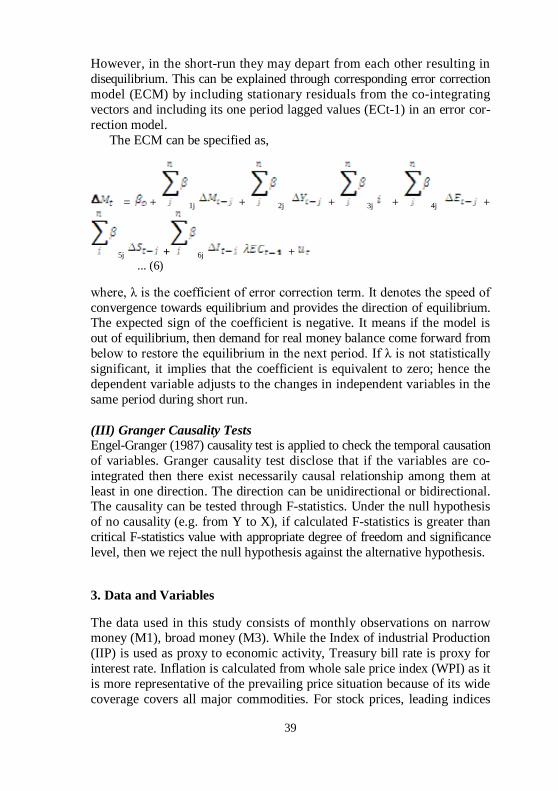
However, in the short-run they may depart from each other resulting in disequilibrium. This can be explained through corresponding error correction model (ECM) by including stationary residuals from the co-integrating vectors and including its one period lagged values (ECt-1) in an error cor- rection model.

The ECM can be specified as,

= + 1j + 2j + 3j + 4j +

5j + 6j + ... (6) where, λ is the coefficient of error correction term. It denotes the speed of convergence towards equilibrium and provides the direction of equilibrium. The expected sign of the coefficient is negative. It means if the model is out of equilibrium, then demand for real money balance come forward from below to restore the equilibrium in the next period. If λ is not statistically significant, it implies that the coefficient is equivalent to zero; hence the dependent variable adjusts to the changes in independent variables in the same period during short run. (III) Granger Causality Tests Engel-Granger (1987) causality test is applied to check the temporal causation of variables. Granger causality test disclose that if the variables are co-integrated then there exist necessarily causal relationship among them at least in one direction. The direction can be unidirectional or bidirectional. The causality can be tested through F-statistics. Under the null hypothesis of no causality (e.g. from Y to X), if calculated F-statistics is greater than critical F-statistics value with appropriate degree of freedom and significance level, then we reject the null hypothesis against the alternative hypothesis.

3. Data and Variables The data used in this study consists of monthly observations on narrow money (M1), broad money (M3). While the Index of industrial Production (IIP) is used as proxy to economic activity, Treasury bill rate is proxy for interest rate. Inflation is calculated from whole sale price index (WPI) as it is more representative of the prevailing price situation because of its wide coverage covers all major commodities. For stock prices, leading indices

40

namely BSE Sensex and S&P Nifty are considered here as these indices are considered to be barometer for the Indian equity market and constitute almost 99% of market capitalization. Since US is major trading and investor partner of India, Rupees per US Dollar is taken for exchange rate. The time series data are collected from the official web site of BSE, NSE, RBI and Ministry of Statistics and Program implementation.

4. Results and Discussions (I) Unit Root Tests results For stationarity testing different tests like ADF, PP and KPSS unit root tests are carried out. The ADF and PP have the null of unit root against an alternative of stationary process. These tests are applied with and without deterministic trend variable in levels to test null of unit root against stationary alternative. The non rejection of the null without trend implies that the series is non stationarity in difference, whereas the rejection with trend indicates that the series is stationary around the deterministic trend. The optimum lag-length is set according to AIC and SIC criteria. To correct serial correlation in error terms, the ADF test adds lagged difference terms of the regress and in error terms, while PP test uses non-parametric methods.

The unit root tests for the data in level form are reported in table-1. The ADF and PP test statistics reported in the table are statistically insignificant and hence the null hypothesis of unit root, without and with trend cannot be rejected for all the six variables. Hence, the all data series are non stationary. The KPSS test results also indicate that the data follows non stationary process at level form as the test statistics are more than critical values. Table-2 presents unit root test statistics for the series at the first difference. In first difference, the null of unit root is rejected by all the three tests carried out here, as tests statistics are highly significant. Hence, unit root tests results show that the chosen variables are non-stationary i.e. integrated of order I (1).

41

Table 1 Unit Root Test Results in Level Variables ADF PP KPSS

Intercept without Trend

Intercept with

Trend

Intercept without Trend

Intercept with

Trend

Intercept without Trend

Intercept with

Trend M3 -0.25610 -2.31294 -0.26723 -2.64481 3.550 0.357 M1 0.01896 -3.28604 0.07255 -3.37884 3.573 0.640 INF 0.89193 -1.78388 0.53667 -2.99875 3.577 0.308 SEN -0.32506 -1.71966 -0.47830 -1.94372 2.953 0.544 NIF -0.39014 -1.90279 -0.50560 -2.11428 3.070 0.503 INR -3.16097 -3.68601 -2.89755 -3.46843 1.628 0.178 USD -1.92484 -1.62795 -2.01016 -1.85057 1.366 0.558 IIP -0.80453 -1.08994 -0.03455 -7.29392 3.525 0.593

The table reports the ADF, PP and KPSS tests statistics in level. The optimal lag for ADF test and truncation lag for PP test are selected based on the AIC and SIC criteria. In the case of both ADF and PP tests, the critical values at 1%, 5% and 10% are –3.46, –2.87 and –2.57, respectively for the model without trend and –4.00, –3.43 and –3.13 for the model with trend. ADF and PP tests examine the null hypothesis of a unit root against the stationary alternative. For fixing the truncation lag for KPSS test, spectral estimation methods selected is the Bartlett kernel, and for bandwidth it is the Newey-West method. The critical values at 1%, 5% and 10% are 0.73, 0.46 and 0.34, respectively for the model without trend and 0.21, 0.14 and 0.11 for the model with trend. The KPSS test examines null of stationarity. * indicates significant at 1% level. Table 2 Unit Root Test Results First Difference

ADF First Difference PP First Difference KPSS Difference

Variables Intercept without Trend

Intercept with

Trend

Intercept without Trend

Intercept with

Trend

Intercept without Trend

Intercept with

Trend M3 -

11.01413* -

10.98408* -

11.01964* -

11.02244* 0.042* 0.042*

M1 -12.80181*

-12.77147*

-12.88993*

-12.89893* 0.042* 0.023*

INF -8.63429* -8.63666* -8.72830* -8.75158* 0.079* 0.028* SEN -

12.49747* -

12.50758* -

12.61767* -

12.65611* 0.096* 0.055*

NIF -12.92496*

-12.92834*

-13.02355*

-13.05881* 0.080* 0.048*

INR -18.91883*

-18.92121*

-18.84595*

-18.92783* 0.082* 0.040*

USD -10.23082*

-10.23570*

-10.27676*

-10.29914* 0.173* 0.076*

IIP -24.19115*

-24.15070*

-25.96794*

-26.08681* 0.048* 0.020*

*denotes the significance of 1%.

42

(II) Co-integration Test Results The association of the variables in the long run can be analyzed with the help of the co-integration test. Johansen and Juselius (1990) method of maximum likelihood principle is carried out in this study. The Johansen method applies the maximum likelihood principle to determine the presence of co-integrating vectors and allows for test of hypothesis regarding elements of the co-integrating vector. Johansen and Juselius (1990) provides two indicators namely trace test and maximum eigen value test to determine the number of co-integrating vectors in the model. Finally, the estimation procedure assumes unrestricted intercepts with no trend in the model. If non-zero vectors are indicated by these tests, a stationary long run relationship exists among the variables. For specifying the co-integration model and estimating the number of co-integrating vector through VAR model it is necessary to specify the number of lags in the autoregressive process. The lag length of 4 is chosen based on log likelihood ratio tests. The test has been conducted with two different stock price indexes alternatively to check the difference.

The obtained results are presented in table-4 (trace test and the maximum eigen value test). Panel-A specify the co-integration equation for the money demand specification M3 and Panel-B specify the co-integration equation for the money demand specification M1. First panel-A present’s co-in- tegration between log real MDF M3, log of output, log of stock prices, log of exchange rate, log of inflation, and the log of short term interest rate is examined. Secondly in panel-B the co-integration among the log of real MDF M1, log of output, log of stock prices, log of exchange rate, log of inflation, and the log of short term interest rate is examined. The results affirmatively support the presence of three co-integrating vectors for MDF M3 and two co-integrating vectors for MDF M1. Both the trace test and maximum eigenvalue test strongly confirm three and two non zero vectors between real MDF M3 and its determinants and real MDF M1 and its determinants. Thus there exists a stationary relationship between real M3 or real M1and output, stock prices, exchange rate, inflation and short term interest rates. In summary, the co-integration test procedure produces a significant stationary long run relationship among the six variables in the model.

Tab

le 3

Joha

nsen

Max

imum

Lik

elih

ood

Test

for C

o-in

tegr

atio

n Pa

nel-A

Pa

nel-B

Hyp

othe

sis

Joha

nsen

max

imum

lik

elih

ood

test

for

Co-

inte

grat

ion

Mon

etar

y V

aria

ble:

Bro

ad

Def

initi

on o

f Mon

ey (M

3)

Stoc

k Pr

ice

Inde

x(Se

nsex

)

Joha

nsen

max

imum

lik

elih

ood

test

for

Co-

inte

grat

ion

Mon

etar

y V

aria

ble:

N

arro

w D

efin

ition

of

Mon

ey (M

1) S

tock

Pri

ce

Inde

x(Se

nsex

)

Joha

nsen

max

imum

lik

elih

ood

test

for

Co-

inte

grat

ion

Mon

etar

y V

aria

ble:

Bro

ad

Def

initi

on o

f Mon

ey (M

3)

Stoc

k Pr

ice

Inde

x(N

ifty)

Joha

nsen

max

imum

lik

elih

ood

test

for

Co-

inte

grat

ion

Mon

etar

y V

aria

ble:

N

arro

w D

efin

ition

of

Mon

ey (M

1) S

tock

Pri

ce

Inde

x(N

ifty)

Nul

l H

ypot

hesi

s A

ltern

ativ

e H

ypot

hesi

s T

race

St

atis

tic

Max

-Eig

en

Stat

istic

T

race

St

atis

tic

Max

-Eig

en

Stat

istic

T

race

St

atis

tic

Max

-Eig

en

Stat

istic

T

race

St

atis

tic

Max

-Eig

en

Stat

istic

r=0

r ≥1

158.

65

68.7

0 14

8.67

65

.68

154.

65

62.9

7 14

2.83

58

.19

r≤1

r≥2

89.9

5 37

.53

82.9

8 39

.58

91.6

8 38

.94

84.6

4 39

.45

r≤2

r≥3

52.4

2 26

.57

43.3

9 27

.18

52.7

3 27

.06

45.1

8 28

.00

r≤3

r≥4

25.8

4 17

.95

16.2

1 7.

48

25.6

6 17

.52

17.1

7 8.

65

r≤4

r≥5

7.89

5.

08

8.73

6.

07

8.14

5.

02

8.52

5.

89

r≤5

r≥6

2.81

2.

81

2.65

2.

65

3.12

3.

12

2.62

2.

62

Not

e: T

he c

ritic

al v

alue

s fo

r tr

ace

test

at 0

.05%

are

95.

75,6

9.81

,47.

85,2

9.79

,15.

49 a

nd 3

.84

and

for

the

max

eig

en s

tatis

tic c

ritic

al v

alue

s ar

e 40

.07,

33

.87,

27.

58, 2

1.13

, 14.

26, a

nd 3

.84

resp

ectiv

ely

43

44

(III) Long Run Elasticities The existence of long-run elasticities in the variables can be captured through the normalized equations which are obtained by dividing each co-integrating vector by the negative of the co-integrating vector on real money balances. These normalised equations are obtained in reduced forms, and can rep- resent money demand and its determinants interactions (Johansen and Juselius 1990). We report the results of implied long-run elasticity in table-4. When M3 is considered as dependent variable, inflation and stock price are ne- gatively and IIP is positively significant at 1percent and 5 percent level (see table-4). However, inflation and interest rate are positively and economic activity and exchange rate are found negatively significant for M1. How- ever, analysis of the results of long run elasticities show that inflation and stock prices are negatively and economic activity is positively significant with respect to M3. Stock prices elasticity, with negative significance indicates that stock prices have a negative wealth effect on money demand for the Indian context. (IV) Error Correction Results Once the co-integration test is conducted and the variables found to have a long run stationary relationship, it implies the variables are co-integrated in long run. If the variables are co-integrated in the long run, it need not necessarily mean that in the short run they are always in equilibrium. The deviation from equilibrium in the short run can be captured through VECM. Generally the error correction term is obtained from the residual terms of co-integrating equation and used into the co-integration equation with the lagged term in first difference. VECM results are presented in table-5. The results reveal that M3 and inflation is positively significant which implies that short run increase in prices will lead to increase in the demand for money, whereas interest rate and IIP are negatively significant in the first lag difference. Furthermore, stock prices have insignificant effect, implying that the coefficients are equal to zero. So the money demand function re- acts to the changes independently in the same period to restore equilibrium. Further, in case of M, inflation is significant in the second lag whereas interest rate, IIP and exchange rate are negatively significant (See table 5). However, the stock prices have insignificant effect on both the M1and M3 in the short run.

Tab

le 4

Lon

g Ru

n El

astic

ities

Dep

ende

nt V

aria

ble:

Ln

(M3)

SP(

Sens

ex)

Dep

ende

nt V

aria

ble:

Ln

(M1)

SP(

Sens

ex)

Dep

ende

nt V

aria

ble:

Ln

(M3)

SP(

Nift

y)

Dep

ende

nt V

aria

ble:

Ln

(M1)

SP(

Nift

y)

Nor

mal

ized

Co-

inte

grat

ing

coef

ficie

nts

Nor

mal

ized

Co-

inte

grat

ing

coef

ficie

nts

Nor

mal

ized

Co-

inte

grat

ing

coef

ficie

nts

Nor

mal

ized

Co-

inte

grat

ing

coef

ficie

nts

Variable

Coefficient

T-Statistic

Variable

Coefficient

T-Statistic

Variable

Coefficient

T-Statistic

Variable

Coefficient

T-Statistic

Ln(I

NF)

-1

7.94

-8

.22*

Ln

(IN

F)

1.37

4.

77*

Ln(I

NF)

-1

7.89

-8

.13*

Ln

(IN

F)

0.99

4.

03*

Ln(I

NR

) -0

.03

-0.1

5 Ln

(IN

R)

0.07

2.

19*

Ln(I

NR

) -0

.11

-0.4

4 Ln

(IN

R)

0.07

2.

74*

Ln(I

P)

13.0

3 7.

69*

Ln(I

P)

-2.2

6 -9

.94*

Ln

(IP)

12

.64

7.51

* Ln

(IP)

-1

.88

-9.9

3*

Ln(S

en)

-0.8

2 -2

.30*

Ln

(Sen

) 0.

02

0.49

Ln

(Nif)

-0

.69

-1.7

7 Ln

(Nif)

0.

02

-0.5

1

Ln(U

SD)

1.19

1.

12

Ln(U

SD)

-0.3

4 -2

.47*

Ln

(USD

) 1.

66

1.60

Ln

(USD

) -0

.34

-3.0

0*

Not

e: *

reje

ctio

n of

nul

l at 1

% le

vels

.

45

Tabl

e 5

Erro

r Cor

rect

ion

Estim

atio

n R

esul

t

Err

or C

orre

ctio

n M

echa

nism

Res

ult:

B

road

Mon

ey D

efin

ition

(M3)

Sto

ck

Pric

e-Se

nsex

Err

or C

orre

ctio

n M

echa

nism

R

esul

t: N

arro

w M

oney

Def

initi

on

(M1)

Sto

ck P

rice

-Sen

sex

Err

or C

orre

ctio

n M

echa

nism

R

esul

t: B

road

Mon

ey D

efin

ition

(M

3) S

tock

Pri

ce-N

ifty

Err

or C

orre

ctio

n M

echa

nism

R

esul

t: N

arro

w M

oney

Def

initi

on

(M1)

Sto

ck P

rice

-Nift

y

Variable

Co-efficient

T-Statistic

Variable

Co-efficient

T-Statistic

Variable

Co-efficient

T-Statistic

Variable

Co-efficient

T-Statistic

m3(

-1)

-0.1

39

-1.5

13

m3(

-1)

-0.1

37

-1.7

32

m3(

-1)

-0.1

37

-1.4

92

m3(

-1)

-0.1

21

-1.5

64

m3(

-2)

-0.0

88

-0.9

44

m3(

-2)

-0.0

44

-0.5

48

m3(

-2)

-0.0

88

-0.9

45

m3(

-2)

-0.0

37

-0.4

76

inf(-

1)

0.41

7 4.

989*

in

f(-1)

0.

060

0.70

9 in

f(-1)

0.

416

4.94

9*

inf(-

1)

0.41

6 5.

264*

inf(-

2)

0.11

2 1.

209

inf(-

2)

0.41

5 5.

317*

in

f(-2)

0.

111

1.18

in

f(-2)

0.

052

0.61

5

inr(-

1)

-0.3

56

-4.4

04*

inr(-

1)

-0.3

58

-4.4

74*

inr(-

1)

-0.3

64

-4.5

12*

inr(-

1)

-0.3

66

-4.6

19*

inr(-

2)

-0.0

01

-0.0

22

inr(-

2)

0.01

8 0.

239

inr(-

2)

-0.0

02

-0.0

25

inr(-

2)

0.01

5 0.

200

ip(-

1)

-0.4

68

-4.5

51*

ip(-

1)

-0.4

32

-3.5

91*

ip(-

1)

-0.4

92

-4.7

82*

ip(-

1)

-0.4

80

-3.9

37*

ip(-

2)

-0.1

05

-1.3

37

ip(-

2)

-0.0

57

-0.6

62

ip(-

2)

-0.1

11

-1.4

03

ip(-

2)

-0.0

72

-0.8

09

sen(

-1)

0.00

0 0.

008

sen(

-1)

-0.0

07

-0.0

90

nif(-

1)

-0.0

39

-0.4

68

nif(-

1)

-0.0

44

-0.5

19

sen(

-2)

0.07

0 0.

827

sen(

-2)

0.07

2 0.

849

nif(-

2)

0.04

7 0.

557

nif(-

2)

0.05

4 0.

639

usd(

-1)

0.24

8 3.

204*

us

d(-1

) 0.

258

3.33

0*

usd(

-1)

0.25

0 3.

210*

us

d(-1

) 0.

263

3.36

5*

usd(

-2)

-0.1

52

-2.0

32*

usd(

-2)

-0.1

53

-2.0

42*

usd(

-2)

-0.1

51

-2.0

18*

usd(

-2)

-0.1

52

-2.0

16*

Not

e: *

and

**

deno

tes t

he si

gnifi

canc

e at 1

% a

nd 5

% le

vel r

espe

ctiv

ely.

46

47

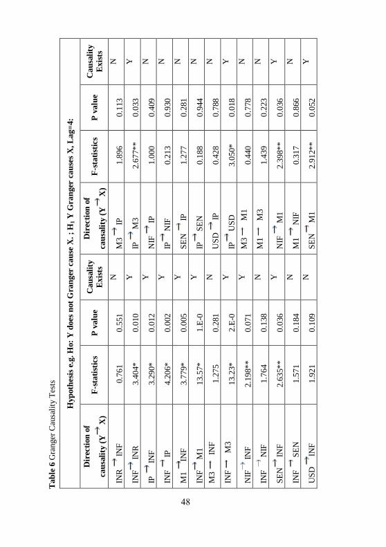
(V) Granger Causality Results The bivariate Granger causality test is applied for testing causal relation- ship among the variables. The Engle and Granger (1987) test states that if the variables are co-integrated, then they must be causally related at least in one direction. The prerequisite for Granger causality is to convert the data series into stationary form via differencing. Further, the test will be carried out on the differenced data series. The bivariate Granger causality test results are reported in table 6. The results corroborates the null hypo- thesis of stock prices does not granger cause monetary aggregates (M1and M2) have been rejected for both the stock price indices proxy viz. Nifty and Sensex at various significance levels. The significance levels are reported through F-statistics and corresponding P values respectively. It implies that the stock prices granger causes money demand but not in reverse man- ner. It further implies that there is unidirectional causality found between stock prices and demand for money. The results are consistent with the theoretical arguments as theory states that as stock prices rise equities become more attractive and the need for demand for money will also rise in order to facilitate the transactions. Further unidirectional causality found from money demand to exchange rate. There is also unidirectional causality from money demand (M1, M2) to interest rate (TBR). It implies that as interest rate reacts for any change in money demand but not in reverse. Further, output is bidirectional related to inflation and narrow demand for money (M1) and unidirectional to interest rate and broad money demand (M2). Demand for money and inflation reported unidirectional causality which implies that there is a reaction of demand for money when inflation change. There is positive relation between demand for money and inflation. In this way the results are consistent and substantiate with the theory, and also justified as per the magnitude and sign of co-efficients are concerned.

Tabl

e 6

Gra

nger

Cau

salit

y Te

sts

Hyp

othe

sis e

.g. H

o: Y

doe

s not

Gra

nger

cau

se X

. ; H

1 Y G

rang

er c

ause

s X, L

ag=4

:

Dir

ectio

n of

caus

ality

(Y X

) F-

stat

istic

s P

valu

e C

ausa

lity

Exist

s D

irec

tion

of

caus

ality

(Y X

) F-

stat

istic

s P

valu

e C

ausa

lity

Exist

s

INR

IN

F 0

.761

0.

551

N

M3

IP

1.8

96

0.11

3 N

INF

INR

3

.404

* 0.

010

Y

IP

M3

2.6

77**

0.

033

Y

IP

INF

3.2

90*

0.01

2 Y

N

IF

IP

1.0

00

0.40

9 N

INF

IP

4.2

06*

0.00

2 Y

IP

NIF

0

.213

0.

930

N

M1

INF

3

.779

* 0.

005

Y

SEN

IP

1

.277

0.

281

N

INF

M1

13.

57*

1.E-

0 Y

IP

SEN

0

.188

0.

944

N

M3

INF

1.2

75

0.28

1 N

U

SD

IP

0.4

28

0.78

8 N

INF

M3

13.

23*

2.E-

0 Y

IP

USD

3

.050

* 0.

018

Y

NIF

INF

2.1

98**

0.

071

Y

M3

M1

0.4

40

0.77

8 N

INF

NIF

1

.764

0.

138

N

M1

M3

1.4

39

0.22

3 N

SEN

INF

2.6

35**

0.

036

Y

NIF

M

1 2

.398

**

0.03

6 Y

INF

SEN

1

.571

0.

184

N

M1

NIF

0

.317

0.

866

N

USD

IN

F 1

.921

0.

109

N

SEN

M1

2.9

12**

0.

052

Y

48

INF

USD

1

.960

0.

103

N

M1

SEN

0

.370

0.

829

N

IP

INR

3

.780

* 0.

005

Y

USD

M1

1.7

73

0.13

6 N

INR

IP

0

.174

0.

951

N

M1

USD

2

.207

**

0.07

0 Y

M1

INR

3

.791

* 0.

005

Y

NIF

M

3 2

.836

**

0.02

3 Y

INR

M

1 0

.304

0.

874

N

M3

NIF

0

.610

0.

655

N

M3

INR

3

.658

* 0.

007

Y

SEN

M3

2.8

20**

0.

053

Y

INR

M

3 0

.038

0.

997

N

M3

SEN

0

.583

0.

674

N

NIF

IN

R

0.4

01

0.80

7 N

U

SD M

3 1

.264

0.

286

N

INR

N

IF

0.3

13

0.86

8 N

M

3 U

SD

0.6

42

0.63

3 N

SEN

IN

R

0.5

48

0.70

0 N

SE

N

NIF

1

.492

0.

206

N

INR

SE

N

0.3

01

0.87

6 N

N

IF S

EN

0.7

18

0.58

0 N

USD

IN

R

0.4

56

0.76

7 N

U

SD

NIF

1

.832

0.

125

N

INR

U

SD

0.5

05

0.73

2 N

N

IF U

SD

3.5

79*

0.00

7 Y

M1

IP

3.0

60*

0.01

8 Y

U

SD S

EN

1.7

42

0.14

3 N

IP

M1

21.

564*

3.

E-1

Y

SEN

USD

3

.735

* 0.

006

Y

*,**

,***

Den

otes

sign

ifica

nce

at 1

%, 5

% a

nd 1

0 re

spec

tivel

y. Y

is fo

r Ye

s an

d N

is fo

r No.

49

50

5. Conclusion The objective of this paper is to estimate the relationship between demand for money, exchange rate and stock prices in India for the period 1996:1 to 2010:8. For the study, two different forms of money demand specifications M1 and M3 are employed. The Johansen and Juselius procedure of co-integration is carried out to test the hypothesis of a stationary relationship between demand for money, real income, the opportunity cost of holding money (short term interest rates) and stock prices. Normalized equations of co-integration are used for the long run elasticity significance and the direction of the effects which are generated or produced by each variable on money demand function. The co-integration results demonstrated more than two co-integrating vectors for both the demand function specifications. Thus, supporting the long-run equilibrium relationship among the variables. The study found that stock prices have negative and significant effect on the money demand and exchange rate found to have negative effect on M1. On the other, economic activity are positively related to M3 and negatively with M1. The stock price is found to have negative wealth effect on long run and short run demand for money.

Further, the short run dynamics are captured by the vector error cor- rection mechanism (VECM). The results reveal that, inflation is positively related to M3 which implies that short run increases in prices will lead to increase in the demand for money, whereas interest rate and IIP are negatively significant in the first lag difference. Further, stock prices have insignificant effect on the demand for broad money in the short run. Be- sides, inflation is significant in the second lag difference with M1 whereas interest rate, IIP and exchange are negatively significant. Unidirectional causality is reported from stock prices to demand for money. Further uni- directional causality found from money demand to exchange rate. There is also unidirectional causality from money demand (M1, M2) to interest rate (TBR). It implies that as interest rate reacts for any change in money demand but not in reverse.

The findings of the study suggest that money demand function estimated is consistent with the theory. All the five variables affect the money demand function with money demand specifications M1 and M3. The paper con- cludes that all the variables significantly affect the money demand function. The empirical evidence of negative wealth effect calls for a tight monetary policy.

51

NOTE

1. Vasudevan (1977) and Arif (1996) provide useful survey of some of the earlier studies.

REFERENCES

Ahluwalia, I. J. (1979), Behavior of Prices & Output in India: A Macro-

Econometric Approach, 1st edn. Mumbai: Macmillan Company of India. Akinlo A. E. (2006), “The Stability of Money Demand in Nigeria: An Auto-

regressive Distributed Lag Approach,” Journal of Policy Modelling 28: 445–452. Arif, R. R. (1996), “Money Demand Stability: Myth or Reality – An Eco-

nometric Analysis,” Development Research Group Study 13, Reserve Bank of India. Avadhani, V. A. (1971), “Money Demand in the Corporate Sector,” Indian

Economic Journal 18: 552–562. Baharumshah A. Z. (2004), “Stock Prices and Long Run Demand for Money

Evidence from Malaysia,” International Economics Journal 18(3): 389–407. Baharumshah A. Z., Mohd S. H., and Yol M. A. (2009), “Stock Prices and

demand for Money in China: New Evidences,” Journal of International Financial Markets Institutions and Money 19: 171–187.

Bahmani-Oskooee, et al. (1991), “Exchange Rate Sensitivity of Demand for Money in Developing Countries,” Applied Economics 23: 1377–1384.

Bahmani-Oskooee, M., and R. Hafez (2005), “Stability of Money Demand Function in Asian Developing Countries,” Applied Economics 37: 773–792.

Bhattacharya, R. (1995), “Co-integrating Relationships in the Demand for Money in India,” The Indian of Economic Journal 43: 69–75.

Bhoi, B. K. (1995), “Modelling Buffer Stock Money: An Indian Experience,” RBI Occasional Papers 16(1).

Biswas, D. (1962), “The Indian Money Market: An Analysis of Money Demand,” Indian Economic Journal 3(9): 308–23.

Carruth A., and Sanchez Fung J. R. (2000), “Money Demand in Dominican Republic,” Applied Economics 32: 1439–1449.

Choudhry T. (1996), “Real Stock Prices and the Long Run Money Demand Function: Evidence from Canada and the U.S.A.,” Journal of International Money and Finance 15: 1–17.

Choudhry T. (1995), “High Inflation Rates and the Long-Run Money Demand Function Evidences from Co-integration Tests”, Journal of Macroeconomics 17(1): 77–91.

Dickey, D. A., and Fuller, W. A. (1976), “Distribution of the Estimations for Autoregressive Time Series with a Unit Root,” Journal of American Statistics Association 74: 427–431.

Engle R. F., and C. W. J Granger (1987), “Co-integration and Error Cor- rection: Representation, Estimation and Testing,” Econometrica 55(2): 251–276.

Friedman, M. (1988), “Money and the Stock Market,” Journal of Political Economy 96: 221–245.

52

Jadav, N. (1994), Monetary Economics for India, 1st edn. Delhi: Macmillan India.

McCornac, D. (1991) “Money and the Level of Stock Market Prices: Evidence from Japan,” Quarterly Journal of Business and Economics 30: 42–51.

Mohanty, D., and Mitra, A. K. (1999), “Experience with Monetary Targeting in India,” Economic and Political Weekly, 16–22/23–29; 34, 3&4, 123–32.

Moosa, I. (1992), “The Demand for Money in India: A Co-integration Ap- proach,” The Indian Economic Journal 40: 101–115.

Muhammad A. H., Khurram A. W., Narjis K., Kashif I. (2009), “Relationship between Stock Prices, Exchange Rate and Demand for Money in Pakistan,” Middle Eastern Finance and Economics 3.

Nag, A. K., and Upadhyay, G. (1993), “Estimation of Money Demand Function: A Co-integration Approach,” Reserve Bank of India Occasional Papers 14: 47–66.

Phillips, P. C. B., and Perron, P. (1988), “Testing for a Unit Root in Time Series Regression,” Econometrica 75: 355–346.

Pradhan, P. C. (2006), “A Co-integration Approach to the Demand for Money under Liquidity Adjustment Facility in India: A Note,” Indian Journal of Economics and Business 5: 78–88.

Pradhan, B. K., and Subramanian, A. (2003), “On the Stability of Demand for Money in a Developing Economy: Some Empirical Issues,” Journal of Develop- ment Economics 72(1): 335–351.

Ramachandran, M. (2004), “Do Broad Money, Output, and Prices Stand for a Stable Relationship in India?” Journal of Policy Modelling 26: 983–1001.

Sampath, R. K., and Hussain, Z. (1981), “Demand for Money in India,” The Indian Economic Journal 24(1): 41–54.

Vasudevan, A. (1977), “Demand for Money in India – A Survey of Literature,” Reserve Bank of India Occasional Papers 2(1): 58–83.

Zuo H., and Park S. Y. (2011), “Money Demand in China and Time Varing Co-integration,” China Economic Review 22: 330–343. © Jyoti Kumari, Jitendra Mahakud

Copyright of Economics, Management & Financial Markets is the property of Addleton Academic Publishers

and its content may not be copied or emailed to multiple sites or posted to a listserv without the copyright

holder's express written permission. However, users may print, download, or email articles for individual use.