EXCHANGE RATES AND THE COMPETITIVENESS OF THE US TIMBER

SECTOR IN A GLOBAL ECONOMY

Adam Daigneault Agr., Env., and Dev. Economics

Ohio State University 2120 Fyffe Rd.

Columbus, OH 43210-1067 Daigneault.3@osu.edu

Brent Sohngen

Agr., Env., and Dev. Economics Ohio State University

2120 Fyffe Rd. Columbus, OH 43210-1067

Sohngen.1@osu.edu

Roger Sedjo Resources For the Future

1616 P St., NW Washington, DC 20036

Sedjo@rff.org

Acknowledgement: Selected Paper prepared for the 2005 meetings of the American Agricultural Economics Association, Providence, Rhode Island. Copyright 2005 by Adam Daigneault, Brent Sohngen, and Roger Sedjo. All rights reserved. Readers may make verbatim copies of this document for non-commercial purposes by any means, provided that this copyright notice appears on all such copies.

ABSTRACT

This paper examines the competitiveness of the US timber industry under different

exchange rate policies using a dynamic optimization model of global timber markets. We

assume that exchange rates affect the cost structure of harvesting and managing forests

and simulate the model for baseline conditions and four additional exchange rate policies.

Two policies consider a strengthening United States dollar scenario and two policies

examine weak South American currencies. Recently South America has increased its

share of global timber production and is shipping increasing quantities of timber to the

Unites States. The results indicate that US competitiveness in the forestry sector is

sensitive both to strong US $ policies and to the weak currency policies pursued by South

American governments. A 20% increase in value of the US $ compared to all other

currencies can reduce harvests by 4 – 7% in the United States over the next 50 years,

while a similar reduction in currency values in South America can reduce U.S.

production by around 0.4%. In dollar terms, each additional cubic meter of wood

produced in South America due to currency policies can reduce producer surplus in the

United States by $100.

INTRODUCTION

Exchange rates can have a large influence on a sector's competitiveness. For a

country experiencing depreciation in the value of its currency, production costs compared

to other regions of the world decline, making its goods more competitive in the global

market. The recent depreciation of the United States dollar (US $) relative to the Euro,

Yen, and Canadian Dollar, for instance, has potentially given U.S. manufacturers a leg-up

in global competition. Empirically, the link between exchange rates and exports in the

forestry sector has been shown by several authors. For example, Uusivuori and

Laaksonen (2001) illustrate that a stronger U.S. dollar in the 1990's led to lower exports

and increased direct investment by US companies in the forest products industries of

competing countries. Hanninen and Toppinen (1999) showed similar results for timber

exports from Finland with fluctuations in their exchange rates.

Although future trends in exchange rates are uncertain, recent exchange rate

adjustments by economies that compete with the United States in the forest products

sector suggests that it is important to consider how future trends in exchange rates may

affect the U.S. forest products industry. There is already concern that the U.S. forest

products industry is facing competitive pressures from abroad due to fundamental

reasons, such as the cost of capital and labor, environmental restrictions, and other factors

(i.e., Lippke et al., 2000; Bumgardner et al., 2004). A recent national timber assessment

by Haynes (2003) projects that the U.S. forest products industry imports more and

exports the same amount over the next 50 years, as foreign competitors gain advantages

from lower production costs and fewer environmental restrictions. Given these concerns,

it is useful to take a more careful look at the potential effects of exchange rate policies on

production and welfare in the U.S. forest products sector.

This paper uses a dynamic global timber market model developed by Sohngen et

al. (1999) to explore the effects of several alternative exchange rate scenarios on the

domestic industry. The model maximizes the net present value of consumers' plus

producer's surplus in global timber markets by optimally managing timberland area,

investments, and age class distributions of 145 forest types in 13 regions worldwide.

Exchange rate policies are modeled adjusting the cost structure of a region's forest

industry (i.e., planting costs, land costs, harvesting costs). Regions experiencing a

declining currency value relative to the rest of the world experience relative reductions in

the costs of producing timber. Changes in costs are assumed to be proportional to

changes in exchange rates in this analysis.

Using a dynamic model of global timber marketsl provides several benefits for

this analysis. First, we are able to monitor changes in investment and harvesting patterns

and timber prices associated with different types of policies. When policies in one region

change, the resulting adjustments in exchange rates can have global effects on

production. It is important to account for responses in all other regions. Second, there

may be non-financial impacts associated with exchange rate adjustments. For instance, if

South America persistently devalues their currency, this could lead to additional

investments in plantation forests or it could lead to additional harvesting in currently

inaccessible tropical rainforests (or both). It is useful from a policy perspective to

understand these non-financial impacts. Third, by utilizing a dynamic optimization

model that manages age classes and investments we are able to assess the relative

influence of exchange rate policies on currently merchantable timber as well as

investments in future stocks of forests. These investments, namely the establishment of

fast-growing timber plantations, have become an important component of the global

timber market and international trade in timber products in the last 30 years.

The baseline scenario in this model assumes that exchange rates are fixed in the

future using an average of those projected by the U.S. Department of Agriculture for the

period 2004-2013 (USDA ERS, 2004). This baseline assumes a relatively strong,

although stable, United State dollar. Two scenarios are then used to assess the effects of

further strengthening in the US $ relative to the rest of the world, following historical

trends in U.S. monetary policy. Two additional scenarios examine weak South American

currencies. South America is chosen because timber production in this region stands as

emerging competition for the US forest products industry. Governments in this region

also have historically pursued weak currency values relative to the United States.

The next section describes the methods used to analyze the effects of exchange

rate adjustments on timber markets. The third section presents the results for a baseline

case and four alternative scenarios that examine how sensitive markets are to adjustments

in long trends in exchange rates. The final section provides a brief summary of the

findings and presents our concluding remarks.

METHODOLOGY

This paper examines the influence of exchange rate policy on investment and

production in industrial timber markets. A global timber market model is utilized to

assess how adjustments in exchange rates influence the cost structure of production in 13

regions world-wide (Table 1). The model is a dynamic optimization model built upon the

earlier work of Sedjo and Lyon (1990) and Sohngen et al. (1999). The current version is

more dis-aggregated and contains more detail on timber production in a number of

regions than the earlier versions.

For the analysis in this paper, we make several simplifying assumptions to

account for adjustments in exchange rates. First, the timber supply model assumes a

single world demand for timber logs with unitary demand elasticity at initial consumption

and prices. This abstracts from a number of the demand-side effects that would occur

with changes in exchange rates. For example, with a "strong" US $, there would be an

increase in demand in US $ denominated countries for all normal goods, while at the

same time a decrease in demand for all non- US $ countries. In this study, we assume

that the terms-of-trade effects are completely offsetting in the worldwide marked for

industrial wood, and hence that aggregate dollar demand for timber is unaffected by our

assumptions on exchange rates. This simplifies the analysis, and it allows us to focus on

modeling regional supply response to exchange rate policies.

Second, we assume that exchange rate policies are introduced and maintained

over long periods of time. This implies that governments are able to pursue policies and

implement them efficiently. This is perhaps somewhat unrealistic given that many

governments in the world change frequently and exchange rates are often determined by

competitive market pressures. Evidence on exchange rates, however, does suggest that

trends in exchange rates can persist for many decades (Figure 1), and that some countries

will under-take substantial re-valuations on world currency markets to align their

exchange rates with domestic interests. To account for sensitivity in how countries adjust

their exchange rates, we model both instantaneous changes in exchange rates, as well as

adjustments in exchange rate trends to try to capture two different types of policy

persistence. Third, we ignore potential volatility in exchange rates, which can also

influence trade (Sun and Zhang, 2003). Future analysis will address the volatility issue

by incorporating stochastic elements into the modeling framework.

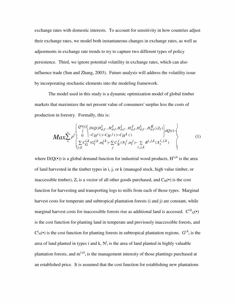
The model used in this study is a dynamic optimization model of global timber

markets that maximizes the net present value of consumers' surplus less the costs of

production in forestry. Formally, this is:

0

1 1 1*( ) ( ( ... , ... , ... ), ), , , , , , ( )( ) ( ) ( )0

, ,, , . , ,( , ) ( , ) ( )

, ,,

I J KQ t D Q H H H H H H Za t a t a t a t a t a t t dQ ti j kt C C CH H H

j j j i j ki k i k i k i j kC G m C N m R Xtt t t tNGi j ki k j

Max ρ

∞−∫

− ⋅ − ⋅ − ⋅

− − ∑

∑ ∑

∑ (1)

where D(Q(▪)) is a global demand function for industrial wood products, Hi,j,k is the area

of land harvested in the timber types in i, j, or k (managed stock, high value timber, or

inaccessible timber), Zt is a vector of all other goods purchased, and CH(▪) is the cost

function for harvesting and transporting logs to mills from each of those types. Marginal

harvest costs for temperate and subtropical plantation forests (i and j) are constant, while

marginal harvest costs for inaccessible forests rise as additional land is accessed. Ci,kG(▪)

is the cost function for planting land in temperate and previously inaccessible forests, and

CjN(▪) is the cost function for planting forests in subtropical plantation regions. Gi,k

t is the

area of land planted in types i and k, Njt is the area of land planted in highly valuable

plantation forests, and mi,j,kt is the management intensity of those plantings purchased at

an established price. It is assumed that the cost function for establishing new plantations

rises as the total area of plantations expands. The total area of land in each forest type is

given as Xi,j,kt, and Ri,j,k(▪) is a rental function for the opportunity costs of maintaining

lands in forests. The rental function represents the supply of land for forestry and is

upward sloping in all regions.

One interesting feature of this model is that both accessible and inaccessible forest

types are modeled. Harvests in inaccessible forests occur if the marginal value of

harvesting a hectare is greater than the marginal access cost of harvesting that hectare.

Exchange rate policies can influence harvests in inaccessible forests by making these

forests, such as tropical rainforests, cheaper to access if tropical countries are pursuing

weak currency valuations. In this analysis, we are able to assess how adjustments in

exchange rate policies influence environmental outcomes, such as harvesting of tropical

timber in regions like South America.

Exchange rate policy is modeled by adjusting the cost structure in the model. The

baseline costs in the model assume a specific set of future exchange rates. These baseline

exchange rates are assumed to remain stable over the entire modeling horizon (150

years). The model is solved in 10 year time increments, and the terminal conditions are

imposed on the system after 150 years. Only the first 50 years are reported in this

analysis.

Alternative exchange rate policies are modeled by applying a scalar adjustment to

all factors of production, CH(▪), Ci,kG(▪), Cj

N(▪), in equation (1) above. When one region’s

currency depreciates (appreciates) relative to another region’s currency, that region’s

costs of production decrease (increase) relative to other regions. To implement exchange

rate adjustments we first calculate a cost adjustment factor for each region j in the model,

shown as αj,t:

,

,

,

( $)

( $)

B

j t

B

t

j t S

j t

S

t

Currency

US

Currency

US

α

=

(2)

In equation (2), the alternative set of future exchange rates, scenarios 1-4, are labeled "S".

If region j's currency is appreciating relative to the US $, then αj,t will be increasing and a

country’s costs will be appreciating relative to costs in the US. The adjustment parameter

αi,t is then incorporated in equation (1) as follows:

0

1 1 1*( ) ( ( ... , ... , ... ), ), , , , , , ( )( ) ( ) ( )0

, ,, , , , ,( , ) ( , ) ( )

, ,,

t t t

t t

I J KQ t D Q H H H H H H Za t a t a t a t a t a t t dQ ti j kt C C CH H H

j j j i j ki k i k i k i j kC G m C N m R Xt t t t tNGi j ki k j

Maxα α α

ρ

α α

∞−∫

− ⋅ − ⋅ − ⋅

− − ∑

∑ ∑

∑ (3)

The baseline scenario (equation 1) and several alternative policy scenarios (equation 3)

are simulated and the results are compared to assess the effects on timber production.

The model aggregates all countries into 13 regions. A number of large economies

are modeled independently, namely the U.S., Canada, Russia, Japan, India, and China.

Europe also is treated as a single region, although a few countries remain outside the

Euro zone. Oceania includes both Australia and New Zealand. These countries are

assumed to advance the same exchange rate policies over time. Other countries are

aggregated into the remaining regions in the model. Currencies for each of these

aggregated regions are chosen based upon the most stable currencies and economies in

each region, as well as their involvement in the timber market (Table 1). In South

America, for example, Brazil accounts for nearly 70 % of the total value harvested

annually. The Brazilian Real is therefore used to simulate exchange rates for all of South

America. For Central Asia, there was little data available on exchange rates for the

region, so the index of “other Asian” currencies developed by the USDA Economic

Research Service (2004) is used.

Figure 1 displays the historical trend and predicted path for the real exchange

rates (local currency per US $) of three major timber supply regions, Europe, Canada,

and South America. These are based upon the USDA Economic Research Service

(2004). The exchange rates used for the 13 regions for the baseline are shown Table 2.

The following four exchange rate scenarios are then analyzed:

• Baseline – All exchange rates are constant

• Scenario 1 - Strong US $, 20% increase over 50 years

• Scenario 2 - Strong US $, instantaneous appreciation of 20%

• Scenario 3 - Weak South America, instantaneous depreciation of 20%

• Scenario 4 - Weak South America, 2% decline per year for 50 years

Scenarios 1 and 2 simulate what might happen if the US $ becomes stronger in

the future through two separate implementations. First, we assume that the US $

strengthens slowly over time. Specifically, scenario 1 assumes that the US $ strengthens

0.4% per year for 50 years. This change is implemented linearly so the entire change over

50 years is 20% relative to the baseline exchange rates in 2000. The 20% increase is then

held constant for the remaining periods in the simulation. Second, we consider an

instantaneous 20% increase in the value of the US $ relative to all other currencies. This

change is assumed to occur in the first time period, and the change remains constant

throughout the entire projection period. Scenarios 3 and 4 examine the influence of

persistently weak currencies in South America. Scenario 3 assumes that South America’s

currency devalues by 20% today relative to all world economies, and maintains this weak

currency valuation throughout the projection period. This is consistent with the large

annual changes experienced in the late 1990's by several South American economies.

Scenario 4 assumes that the South American currency weakens 2% per year for 50 years,

and then holds constant. Over the past 30 years, Brazil’s currency depreciated an average

of 4.4% per year, while Argentina’s weakened by an average of 7.7%; thus this rate of

change is not unrealistic for a long term scenario analysis.

RESULTS

The baseline results indicate that global timber prices (denominated in 2000 real

Southern US softwood log prices) rise from $114 per m3 to $132 per m3 from 2000 to

2050, an increase of 0.3% per year. Total quantity of timber produced increases only

slightly over this time period, from 1.64 billion m3 to 1.71 billion m3 per year. Historical

timber harvests for a number of major timber producing regions in the model for 1961 to

2000, as well as projections to 2050 for the baseline scenario are shown in Figure 2.

Timber production in the United States and Canada are projected to decline over the next

half century, while production in Europe expands. Timber production in South America

and Oceania, two emerging subtropical plantation regions, steadily increase over time.

In the future, timber supply is projected increasingly to be derived from industrial

wood plantations located in sub-tropical regions, including the Southern U.S., Australia,

New Zealand, South America, Asia, and Africa. In comparison to many temperate

forests that grow at 2 – 5 m3 per hectare per year, industrial subtropical plantations often

grow at 10 – 15 m3 per hectare per year. The total area of these fast-growing plantations

expands from around 70 million hectares currently to around 130 million hectares in

2050. Total wood production increases from about 200 million m3 per year, or about

13% of total wood supply, to about 700 million m3, or about 41% of total wood supply by

2050. There is enough productive land in subtropical regions, and land rental costs are

low enough, to justify the costs of additional establishments despite relatively modest

price increases.

As a result of increasing establishment of fast-growing industrial wood

plantations, South America is projected to continue expanding its market share,

experiencing an annual increase in production of approximately 0.8% per year over the

next 50 years. Under the baseline, most of these increases are derived from harvests in

industrial wood plantations. The area of land devoted to plantations in South America is

projected to more than double during the coming half century, from 10.7 million hectares

to 26.7 million hectares in 2050. Although total harvests increase in the region, baseline

harvests from natural tropical and subtropical forests are projected to decline over the

next 50 years. Industrial wood plantations are projected to account for as much as 71%

of the timber harvested from South America by 2050.

The results of the scenarios on timber production for the world's major timber

producing regions are shown in table 4. Average annual timber production over the 50

year period from 2000 – 2050 is shown in the first column. The stronger US $ scenarios,

not surprisingly, have a negative effect on timber production in the United States. A

0.4% annual increase in the value of the US $ relative to other currencies could reduce

domestic timber production over the next 50 years by 3.8%. The net present value of

producer surplus in the U.S. market over the 50 year period, where producer surplus is

calculated as the value of timber production less costs, declines by 2.2%. The 12 other

timber producing regions have gains in total production and producer surplus. The 20%

instantaneous increase in the value of the US $ relative to other currencies reduces US

production over the next 50 years by 7.2%. The net present value of producer surplus

declines by 8.6%. All other regions experience gains in timber production and increases

in producer surplus, with the exception of Europe. South America and Oceania gain the

most.

The Southern U.S. is heavily affected by the strong US $ scenarios. The area of

pine plantations is expected to increase by about 2.0 million hectares in the baseline over

the next 50 years, totaling 14.1 million in 2050. Results suggest that the area devoted to

these plantations decreases approximately 2% (0.2 million hectares) relative to the

baseline for both scenarios. As a result of the reduction in timberland area, timber

production in the US South declines 0.1% relative to the baseline, which translates to a

loss of about $500 million in producer surplus. While the overall reduction in timber

harvests is greatest in the South, the Northeast and the Great Lakes are hurt the most in

percentage terms, as annual harvests in that region decline 8% to 15% relative to the

baseline over the period.

The 20% instantaneous devaluation of South America's currency relative to the

rest of the world (scenario 3) increases timber production in that region by 6.9%. This

amounts to an additional 14 million m3 of industrial timber harvests per year over the

next 50 years. The net present value of producer surplus in South America increases by

$17.6 billion. Weaker currency valuations could potentially attract substantial additional

foreign direct investment into that region. For scenario 3, the instantaneous reduction in

the value of South American currencies relative to the rest of the world has a proportional

impact upon harvests in different timber types. Plantation harvests increase by a similar

percentage (+6.4%), as harvests in natural tropical and subtropical forests (+7.5%). By

2050, more than 70% of regional harvests were from industrial wood plantations, up from

31% in 2000.

Implementing a 2% per year reduction in the value of South American currencies

relative to the rest of the world over a 50 year period (which is a stronger overall change

over the next 50 years than scenario 3) suggests a 14.2% increase in timber harvests, or

29 million m3 per year additional harvesting. This results in additional net present value

of producer surplus of $32 billion. Harvests in natural tropical and subtropical forests

increase by 29% compared to a 2.4% increase in harvests in plantations. Under the

stronger assumptions of this scenario, the proportional change in harvests from natural

forests is larger than scenario 3. Inaccessible forests are by definition marginal, so that

the reduction in the relative costs of access to these forests has a large effect on

harvesting. Weakening currency valuations in South America can have potentially

important environmental consequences if these harvests are not conducted in

environmentally sound ways.

Increasing harvests in South America causes production in the United States to

decline. On average, for every additional 10 - 13 m3 per year harvested in South

America, 1 m3 less wood is harvested in the United States under these scenarios. The

largest effects occur in the Great Lakes and Northeastern states, which experience

reductions in timber harvests of 2% - 7% over the period 2000 – 2050 depending on the

scenario. All other regions experience a reduction of 1% or less. Costs of production per

m3 of wood harvested tend to be higher in these more northerly regions in the United

States, which implies that these regions are most vulnerable to exchange rate policies

undertaken by South America.

CONCLUSIONS

This paper examines the influence of exchange rate policies on timber production

in the United States and South America. Capital intensive industries, such as forestry,

have been shown to be fairly sensitive to exchange rates (Uusivuori and Laaksonen,

2001; Hanninen and Toppinen, 1999). Although in the past couple years the US $ has

declined in value relative to many currencies, the historically stated monetary policy of

the US government is to pursue a strong US $ relative to other currencies. A strong US $

can weaken the comparative advantage of US industries competing in a global market. In

addition to assessing a strong US $, we also consider the effects of weak South American

currencies. Historical data indicates that the currencies of countries in South America

have depreciated 4 % to 7% per year on average over the past 30 years as these countries

have pursued policies that maintain the competitiveness of their products on world

markets. These policies appear to have been successful at least to some extent as

harvests from South America have increased with continued extraction from inaccessible

tropical forests, and the establishment of fast-growing industrial wood plantations on old

agricultural land.

To address the effects of exchange rate policies on timber production, we adopt

the global timber market model described in Sedjo and Lyon (1990) and Sohngen et al.

(1999). The model uses dynamic programming to simulate optimal harvesting,

management, and regeneration intensity in 150 timber types throughout the world.

Exchange rate policies are introduced by adjusting the cost structure in the model.

Depending on the scenario, the costs of harvesting, accessing, regenerating and holding

forests in each region are adjusted to account for relative changes in costs caused by

changes in exchange rates over time.

In addition to the baseline, four scenarios are considered. Scenarios 1 and 2

examine a strong US $ policy. The first scenario assumes that the US $ gradually

becomes stronger by 20% relative to current exchange rates over the next 50 years. The

second scenario assumes that the US $ instantaneously becomes stronger in the first

period by 20% relative to the current exchange rates. Scenarios 3 and 4 consider weak

South American currency valuations. Scenario 3 considers an instantaneous 20%

reduction in the value of South American currencies, simulating the devaluations that

occurred in the late 1990's. Scenario 4 assumes that the devaluation trends of the past 30

years continue over the next 50 years and then stabilize.

The results indicate that additional strengthening of the US $ relative to the rest of

the world could have substantial impacts upon the competitiveness of the US forest

products industry. A 20% increase in the value of the dollar would lead to a 4-7%

reduction in timber production in the U.S., depending on whether the strengthening

occurs earlier rather than later, and a 2– 9% reduction in producer surplus (welfare) in the

U.S. timber sector. The Great Lakes and Northeastern U.S. are the most heavily affected

regions by the policy. These regions tend to have higher costs and lower growth rates,

and therefore are less able to adapt. Pine plantations in the Southern U.S. are expected to

continue gaining ground in the U.S. marketplace, but the exchange rate policies do reduce

overall establishment over the next 50 years by 200,000 – 300,000 hectares.

The results indicate that if South America continues to pursue weak currency

valuations, their timber products sector will benefit. Under scenario 3 (a 20%

instantaneous reduction in the value of South American currencies relative to the rest of

the world), timber harvests in South America increase by 7% relative to the baseline.

Scenario 4 assumes smaller changes in exchange rates over the next half century than

observed over the past 30 years, but this scenario stimulates substantial additional

harvesting in South America compared to the baseline. Under this scenario, production

in South America increases by 14% per year on average over the next half century.

Producer surplus for the region increases by $18 billion in scenario 3 and $33 billion in

scenario, changing by 7 % and 12 %, respectively. Each additional 10 m3 of timber

harvested in South America reduces production in the United States by 1 m3 under these

exchange rate policies. Portrayed by monetary terms, each 1 m3 increase in timber

production in South American caused by the weak currency policy reduces producer

surplus by about $100 in the United States. As with the strong US $ scenarios,

production in northern parts of the U.S. is affected most heavily by weak South American

currencies.

In addition to potential financial effects, currency policies can influence

environmental outcomes. Under scenarios 3 and 4, timber harvests in plantations and

natural tropical forests both increase. However, under scenario 4 there are substantial

projected increases in harvests in natural tropical forests. This makes sense because these

are marginal supply regions and as such any reductions in access costs can have large

effects on supply.

REFERENCES

Bumgardner M, U. Buehlmann, A. Schuler, and R. Christianson. 2004. “Domestic competitiveness in secondary wood industries,” Forest Products Journal, 54(10): 21-28. Hanninen R, and A Toppinen. 1999. “Long-run Price Effects of Exchange Rate Changes in Finnish Pulp and Paper Exports,” Applied Economics, 31(8): 947-56. Haynes, R. 2003. “An Analysis of the Timber Situation in the United States: 1952-2050,” USDA Forest Service, Pacific Northwest Research Station. General Technical Report. PNW-GTR-560. 254p. Lippke, B, R. Braden, and S. Marshall. 2000. "Export Trends and the Health of the Pacific Northwest Forest Sector," Working Paper 75. Center for International Trade in Forest Products. University of Washington. Sedjo, R. and K. Lyon. The Long-Term Adequacy of World Timber Supply. Washington D.C: Resources for the Future, 1990. Sohngen, B., R. Mendelsohn, and R. Sedjo. 1999. “Forest Management, Conservation, and Global Timber Markets,” American Journal of Agricultural Economics. 81:1-13. Sun C, and DW Zhang. 2003. “The Effects of Exchange Rate Volatility on US Forest Commodities Exports,” Forest Science, 49(5): 807-14. USDA Economic Research Service. 2004. “Economic Research Service Exchange Rate Data Set,” ed. M. Shane. www.ers.usda.gov/data/exchangerates/ US Dept of Treasury. 2004. “Treasury Reporting Rates of Exchange,” updated Nov ’04. http://www.fms.treas.gov/intn.html Uusivuori J, and C.S. Laaksonen. 2001. “Foreign Direct Investment, Exports and

Exchange Rates: The Case of Forest Industries,” Forest Science, 47(4): 577-86.

Table 1 - Currencies used for exchange rate in 13 regions

Region Currency/Currencies used

USA United States Dollar

Canada Canadian Dollar

South America Brazilian Real

Central America Mexican Peso

Europe Euro

Russia Russian Ruble

China Chinese Yuan

India Indian Rupee

Oceania Australian Dollar

SE Asia Malaysian Ringgit

Central Asia Index of Central Asian Countries

Japan Japanese Yen

Africa South African Rand

Table 2 – Exchange Rates for Baseline Case

Exchange Rate (Sept '04)* Exchange Rate (Baseline)

(LC/US$) (LC/US$)

US 1.00 1.00

CA 1.31 1.25

SA 2.93 3.33

CENA 11.38 10.09

EU 0.82 0.87

FSU 29.25 25.66

CH 8.27 6.90

IN 46.18 54.12

OC 1.41 1.37

SEA 3.80 3.88

CAS 103.52 114.35

JAP 108.82 98.41AF 6.64 5.88

*source: US Treasure Dept, 2004

Table 4: Effects of exchange rate policies on annual average production (2000 – 2050).

Baseline Scenario 1 Scenario 2 Scenario 3 Scenario 4

Mm3/yr Mm3/yr % Mm3/yr % Mm3/yr % Mm3/yr %

U.S. 325.9 313.4 -3.8% 302.4 -7.2% 324.6 -0.4% 323.8 -0.6%

Canada 163.6 163.8 0.1% 164.0 0.2% 163.8 0.1% 162.7 -0.5%

S. America 203.9 204.5 0.3% 205.0 0.5% 218.0 6.9% 233.0 14.2%

C. America 17.5 17.5 0.1% 17.6 0.7% 17.4 -0.4% 17.4 -0.7%

Europe 352.7 354.2 0.4% 350.1 -0.7% 343.7 -2.6% 344.0 -2.5%

Russia 97.8 99.1 1.3% 99.7 1.9% 97.4 -0.4% 97.7 -0.1%

China 137.8 138.8 0.7% 142.5 3.4% 135.4 -1.7% 137.0 -0.6%

India 36.7 36.8 0.2% 36.9 0.5% 36.7 -0.1% 36.6 -0.4%

Oceania 84.2 84.5 0.4% 84.9 0.8% 83.9 -0.4% 83.2 -1.2%

SE Asia 124.3 124.4 0.1% 126.6 1.9% 124.3 0.0% 124.1 -0.1%

Cent. Asia 17.7 17.8 0.5% 17.8 0.5% 17.7 -0.1% 17.6 -0.9%

Japan 59.3 58.9 0.1% 58.9 0.1% 58.9 0.1% 58.8 0.0%

Africa 55.0 55.2 0.5% 55.3 0.6% 54.9 0.1% 54.7 -0.5%

Total 1676.0 1668.8 -0.4% 1661.7 -0.9% 1676.6 0.0% 1690.5 0.9%

Table 5: Effects of exchange rate policies on NPV (r=0.05) producer surplus (2000 – 2150).

Baseline Scenario 1 Scenario 2 Scenario 3 Scenario 4

Billion $

Billion $ %

Billion $ %

Billion $ %

Billion $ %

U.S. 531.8 520.0 -2.2% 486.3 -8.6% 532.2 0.1% 528.7 -0.6%

Canada 255.2 255.5 0.1% 256.9 0.7% 255.4 0.1% 253.7 -0.6%

S. America 241.8 242.4 0.2% 243.4 0.7% 259.4 7.3% 274.2 13.4%

C. America 18.8 18.8 0.0% 18.9 0.5% 18.8 0.0% 18.6 -1.1%

Europe 537.6 538.6 0.2% 540.5 0.5% 474.8 -11.7% 533.9 -0.7%

Russia 134.1 134.1 0.0% 135.1 0.8% 134.2 0.1% 133.1 -0.8%

China 160.3 160.8 0.3% 161.3 0.6% 160.3 0.0% 158.9 -0.9%

India 29.1 29.2 0.3% 29.3 0.7% 29.1 0.0% 28.6 -1.7%

Oceania 52.7 53.1 0.8% 53.3 1.1% 52.7 0.0% 51.7 -1.9%

SE Asia 114.8 115.1 0.3% 115.6 0.7% 114.8 0.0% 113.6 -1.0%

Cent. Asia 12.3 12.4 0.8% 12.5 1.6% 12.3 0.0% 12.1 -1.6%

Japan 49.6 49.7 0.2% 50.1 1.0% 49.7 0.2% 49.1 -1.0%

Africa 97.2 97.4 0.2% 97.7 0.5% 97.3 0.1% 96.6 -0.6%

Total 2235.3 2227.1 -0.4% 2200.8 -1.5% 2190.8 -2.0% 2252.8 0.8%

Figure 1 - Historical and projected real exchange rates of selected timber supply regions, 1971-2013

0.00

0.50

1.00

1.50

2.00

2.50

3.00

1971 1975 1979 1983 1987 1991 1995 1999 2003 2007 2011

Year

Lo

cal

Cu

rren

cy /

US

$ (

base =

2000)

Canada

Europe

South America

Figure 2 – Historical and projected timber supply by region, 1961-2050

0

100

200

300

400

500

600

700

800

900

1961 1970 1980 1990 2000 2010 2020 2030 2040 2050

year

millio

n c

ub

ic m

ete

rs

Rest of World

United States

Europe

South America

Canada