term numerical forecasts using windtracer® lidar data

1

SHORT-‐TERM NUMERICAL FORECASTS USING WINDTRACER® LIDAR DATA

Richard L. Carpenter, Jr., and Brent L. Shaw Weather Decision Technologies, Inc., Norman, Oklahoma, USA

Michael Margulis, Keith S. Barr, Tahllee Baynard, Rod Munson, and Pete Wanninger

Lockheed Martin Coherent Technologies Louisville, CO

Devon Yates

NaturEner USA, LLC San Francisco, CA

Stanton L. Thomas

One Network Enterprises Dallas, TX

Justin Sharp

Sharply Focused LLC Portland, OR

ABSTRACT

The Lockheed Martin WindTracer® lidar provides dense coverage of winds over a large volume (typically 15 km horizontally from the lidar and throughout much of the troposphere), making it well suited for use in forecasting for wind energy. During the summer of 2013, two WindTracer® lidars were operated in tandem near a Montana wind farm. The data were incorporated into two models: a simple advection-‐based model, and the WRF mesoscale model, with the goal of significantly improving 0–2 h wind forecasts. WindTracer® data were assimilated into WRF using Four Dimensional Data Assimilation (FDDA) and were also used during post-‐processing to remove model biases. Results indicate the considerable value of incorporating WindTracer® data.

1. OVERVIEW

Boundary-‐layer observations are critically needed for wind energy forecasting. We describe a study in which Lockheed Martin Coherent Technologies (LMCT) WindTracer® Doppler lidar data were incorporated into two short-‐term forecast models with the specific goal of improving 0–2 hour wind forecasts. These forecast models were (1) a simple advection-‐based model and (2) the Weather Research and Forecasting Model (WRF). Lidar data were ingested directly into WRF during

data assimilation as well as post-‐processing phases.

The WindTracer® Doppler lidar transmits at an eye-‐safe invisible infrared frequency of 1.6 μm. It scans in azimuth and elevation to retrieve wind vectors throughout a 3D volume. The coverage radius typically extends to 15 km, depending on the concentration of aerosol backscatters and precipitation. Data are obtained on radials with a typical gate spacing of < 70 m. WindTracer® is also used for aviation safety, defense, security, and research applications.

4th Conf. Weather, Climate, New Energy Economy AMS, 7-‐10 January 2013, Austin, TX

2

2. WindTracer® Operation at Glacier Wind Farm

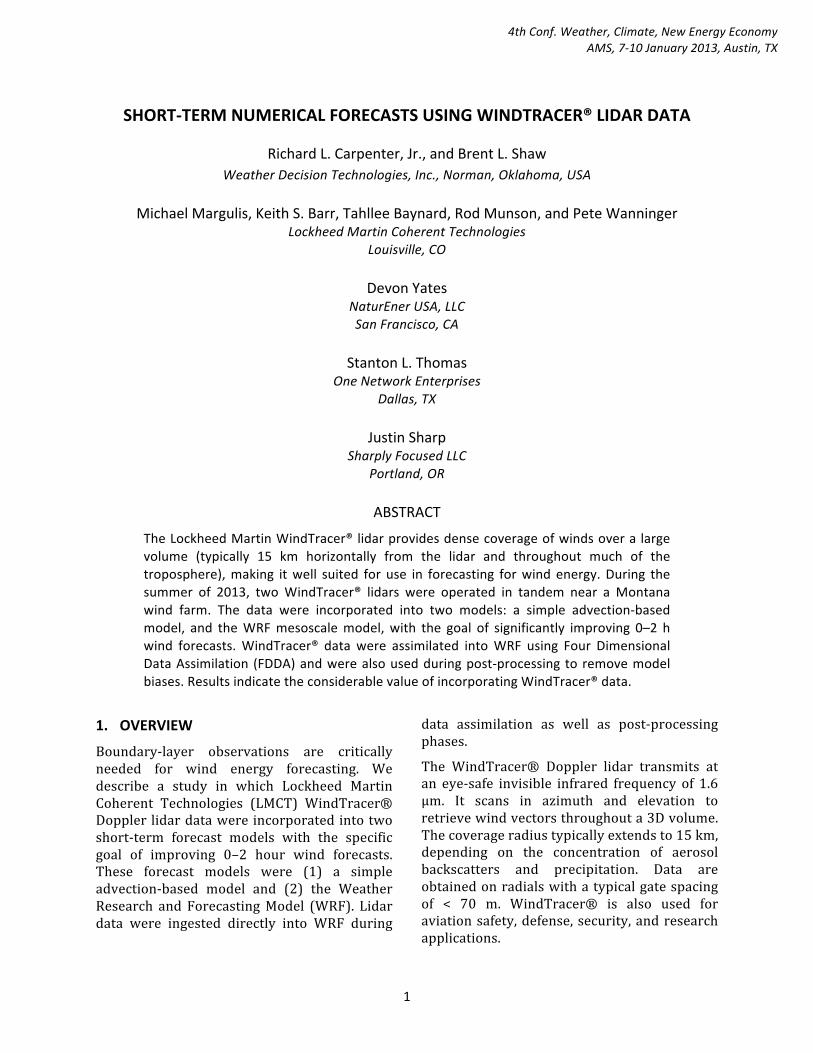
For this study, two WindTracer® lidars were sited near the Glacier Wind Farm (GW) near Ethridge, MT, which is owned and operated by NaturEner USA, LLC (Figure 1). At this location westerly winds commonly advance eastward from the Rockies during the morning as the atmosphere destabilizes. The lidars were therefore sited upwind of GW in order to capture this phenomenon.

During the course of this study, which occurred during the summer of 2012, two other significant weather phenomena were identified. First, cold fronts and thunderstorm outflows frequently traveled southward across the study area. Second, a stable surface layer sometimes remained over GW, but not over the higher elevation to the west. This was manifested by westerly winds just west of GW and southeasterly winds over GW and locations to the east.

WindTracer typically performs a volumetric update in 5-‐10 min. For this project, volume scans consisting of 6 elevation angles were completed in 10 min. Five of the scan angles

ranged from ±1° and were optimized to detect the wind at hub height (80 m) above each turbine location. The sixth scan was at 45° for monitoring upper-‐level winds up to about 8 km above ground level (AGL).

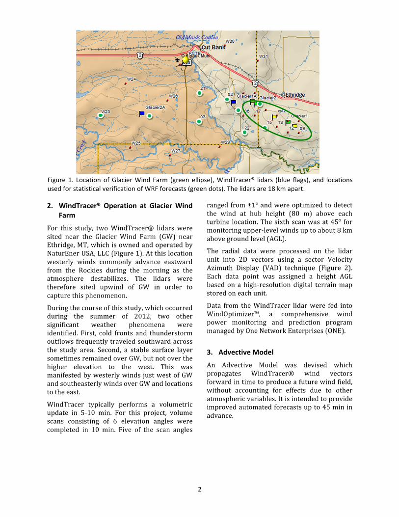
The radial data were processed on the lidar unit into 2D vectors using a sector Velocity Azimuth Display (VAD) technique (Figure 2). Each data point was assigned a height AGL based on a high-‐resolution digital terrain map stored on each unit.

Data from the WindTracer lidar were fed into WindOptimizer™, a comprehensive wind power monitoring and prediction program managed by One Network Enterprises (ONE).

3. Advective Model

An Advective Model was devised which propagates WindTracer® wind vectors forward in time to produce a future wind field, without accounting for effects due to other atmospheric variables. It is intended to provide improved automated forecasts up to 45 min in advance.

Figure 1. Location of Glacier Wind Farm (green ellipse), WindTracer® lidars (blue flags), and locations used for statistical verification of WRF forecasts (green dots). The lidars are 18 km apart.

3

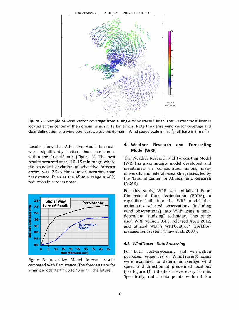
Results show that Advective Model forecasts were significantly better than persistence within the first 45 min (Figure 3). The best results occurred at the 10–15 min range, where the standard deviation of advective forecast errors was 2.5–6 times more accurate than persistence. Even at the 45-‐min range a 40% reduction in error is noted.

Figure 3. Advective Model forecast results compared with Persistence. The forecasts are for 5-‐min periods starting 5 to 45 min in the future.

4. Weather Research and Forecasting Model (WRF)

The Weather Research and Forecasting Model (WRF) is a community model developed and maintained via collaboration among many university and federal research agencies, led by the National Center for Atmospheric Research (NCAR).

For this study, WRF was initialized Four-‐Dimensional Data Assimilation (FDDA), a capability built into the WRF model that assimilates selected observations (including wind observations) into WRF using a time-‐dependent “nudging” technique. This study used WRF version 3.4.0, released April 2012, and utilized WDT’s WRFControl™ workflow management system (Shaw et al., 2009).

4.1. WindTracer® Data Processing

For both post-‐processing and verification purposes, sequences of WindTracer® scans were examined to determine average wind speed and direction at predefined locations (see Figure 1) at the 80-‐m level every 10 min. Specifically, radial data points within 1 km

Figure 2. Example of wind vector coverage from a single WindTracer® lidar. The westernmost lidar is located at the center of the domain, which is 18 km across. Note the dense wind vector coverage and clear delineation of a wind boundary across the domain. (Wind speed scale in m s–1; full barb is 5 m s–1.)

4

horizontally, 10 m vertically, and 5 min temporally were averaged to each location. For quality control purposes, locations having fewer than a specified number of lidar observations are rejected.

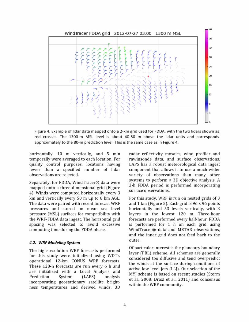
Separately, for FDDA, WindTracer® data were mapped onto a three-‐dimensional grid (Figure 4). Winds were computed horizontally every 3 km and vertically every 50 m up to 8 km AGL. The data were paired with recent forecast WRF pressures and stored on mean sea level pressure (MSL) surfaces for compatibility with the WRF-‐FDDA data ingest. The horizontal grid spacing was selected to avoid excessive computing time during the FDDA phase.

4.2. WRF Modeling System

The high-‐resolution WRF forecasts performed for this study were initialized using WDT’s operational 12-‐km CONUS WRF forecasts. These 120-‐h forecasts are run every 6 h and are initialized with a Local Analysis and Prediction System (LAPS) analysis incorporating geostationary satellite bright-‐ness temperatures and derived winds, 3D

radar reflectivity mosaics, wind profiler and rawinsonde data, and surface observations. LAPS has a robust meteorological data ingest component that allows it to use a much wider variety of observations than many other systems to perform a 3D objective analysis. A 3-‐h FDDA period is performed incorporating surface observations.

For this study, WRF is run on nested grids of 3 and 1 km (Figure 5). Each grid is 96 x 96 points horizontally and 53 levels vertically, with 3 layers in the lowest 120 m. Three-‐hour forecasts are performed every half-‐hour. FDDA is performed for 1 h on each grid using WindTracer® data and METAR observations, and the inner grid does not feed back to the outer.

Of particular interest is the planetary boundary layer (PBL) scheme. All schemes are generally considered too diffusive and tend overpredict the winds at the surface during conditions of active low level jets (LLJ). Our selection of the MYJ scheme is based on recent studies (Storm et al., 2008; Draxl et al., 2011) and consensus within the WRF community.

Figure 4. Example of lidar data mapped onto a 2-‐km grid used for FDDA, with the two lidars shown as red crosses. The 1300-‐m MSL level is about 40-‐50 m above the lidar units and corresponds approximately to the 80-‐m prediction level. This is the same case as in Figure 4.

5

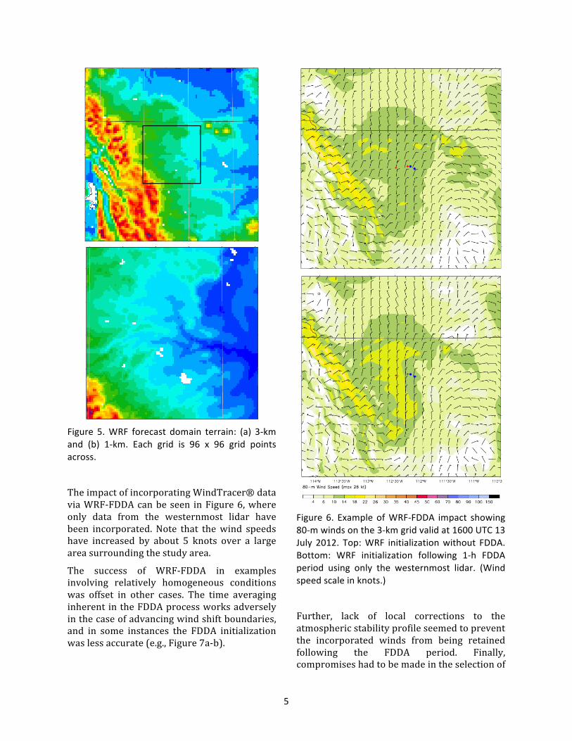
Figure 5. WRF forecast domain terrain: (a) 3-‐km and (b) 1-‐km. Each grid is 96 x 96 grid points across.

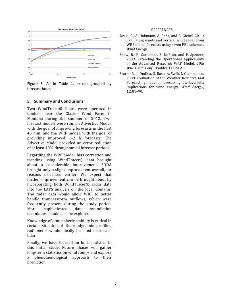
The impact of incorporating WindTracer® data via WRF-‐FDDA can be seen in Figure 6, where only data from the westernmost lidar have been incorporated. Note that the wind speeds have increased by about 5 knots over a large area surrounding the study area.

The success of WRF-‐FDDA in examples involving relatively homogeneous conditions was offset in other cases. The time averaging inherent in the FDDA process works adversely in the case of advancing wind shift boundaries, and in some instances the FDDA initialization was less accurate (e.g., Figure 7a-‐b).

Figure 6. Example of WRF-‐FDDA impact showing 80-‐m winds on the 3-‐km grid valid at 1600 UTC 13 July 2012. Top: WRF initialization without FDDA. Bottom: WRF initialization following 1-‐h FDDA period using only the westernmost lidar. (Wind speed scale in knots.)

Further, lack of local corrections to the atmospheric stability profile seemed to prevent the incorporated winds from being retained following the FDDA period. Finally, compromises had to be made in the selection of

6

FDDA parameters to avoid overfitting the data. Thus, while FDDA performs well on larger-‐scale domains with comparatively evenly spaced data, its value was limited in this study in which a high density of observations was concentrated over a relatively small region.

4.3. Post-‐Processing Using WindTracer® Data

WindTracer® data was incorporated into a three-‐phase post-‐processing procedure (Figure 7b-‐c). First, simple bias correction was used owing to its simplicity, robustness, and ability to explain much of the error variance. Biases were computed per location and per valid hour of the day. Biases were recomputed each day based on the verification of the previous 15-‐day period.

Second, temporal smoothing was performed to remove high-‐frequency signals. Finally, the forecast was trended to WindTracer® observa-‐tions by setting the initial forecast equal to the most recent observation and tapering the difference over a 1-‐hour period.

4.4. WRF Results

Overall WRF forecast results are presented in Table 1, based on entire 3-‐h forecasts on the 3-‐km grid over 59 days in the summer of 2012. Quiescent periods have been filtered out by selecting the 44% of forecasts during which the observed wind speed varied by more than 4 m s–1.

Bias correction and trending considerably improve the forecasts. The improvement based on FDDA is much smaller, for reasons cited earlier. (Results from the 1-‐km grid are similar, although they would have been expected to be somewhat better.)

The impact of bias correction and trending is strongest during the first forecast hour (Figure 8). All of the forecasts are better than persistence after the first hour or so.

Figure 7. Example of forecast improvement using FDDA and bias correction/trending. WindTracer® observations at a particular location are indicated by a black line and shading. Series of 3-‐h WRF forecasts, initialized every 30 min, are shown by colored lines. (a) Uncorrected WRF forecasts. (b) WRF with WindTracer® FDDA. (c) WRF with FDDA and bias correction/trending. Same case as Figures 2 and 4.

Model Bias MAE St Dev WRF –0.4 2.2 2.9 +FDDA –0.4 2.1 2.8 +Bias Correction/ Trending

0.1 1.7 2.4

Persistence –0.0 1.8 2.6

Table 1. Overall 3-‐km WRF forecast results for the period 26 June – 23 Aug 2012. Results cover 44% of forecasts during which the observed wind speed varied by more than 4 m s–1.

7

Figure 8. As in Table 1, except grouped by forecast hour.

5. Summary and Conclusions

Two WindTracer® lidars were operated in tandem near the Glacier Wind Farm in Montana during the summer of 2012. Two forecast models were run: an Advective Model, with the goal of improving forecasts in the first 45 min; and the WRF model, with the goal of providing improved 1–2 h forecasts. The Advective Model provided an error reduction of at least 40% throughout all forecast periods.

Regarding the WRF model, bias correction and trending using WindTracer® data brought about a considerable improvement. FDDA brought only a slight improvement overall, for reasons discussed earlier. We expect that further improvement can be brought about by incorporating both WindTracer® radar data into the LAPS analysis on the local domains. The radar data would allow WRF to better handle thunderstorm outflows, which were frequently present during the study period. More sophisticated data assimilation techniques should also be explored.

Knowledge of atmospheric stability is critical in certain situation. A thermodynamic profiling radiometer would ideally be sited near each lidar.

Finally, we have focused on bulk statistics in this initial study. Future phases will gather long-‐term statistics on wind ramps and explore a phenomenological approach to their prediction.

REFERENCES Draxl, C., A. Hahmann, A. Peña, and G. Giebel, 2011:

Evaluating winds and vertical wind shear from WRF model forecasts using seven PBL schemes. Wind Energy.

Shaw, B., R. Carpenter, Z. DuFran, and P. Spencer, 2009: Extending the Operational Applicability of the Advanced Research WRF Model. 10th WRF Users’ Conf., Boulder, CO, NCAR.

Storm, B., J. Dudhia, S. Basu, A. Swift, I. Giammanco, 2008: Evaluation of the Weather Research and Forecasting model on forecasting low-‐level jets: Implications for wind energy. Wind Energy, 12:81–90.

term numerical forecasts using windtracer® lidar data

Documents

Transcript of term numerical forecasts using windtracer® lidar data