Seasonal forecasts of drought indices in African basins

HESSD9, 11093–11129, 2012

Seasonal forecastsof drought indices in

African basins

E. Dutra et al.

Title Page

Abstract Introduction

Conclusions References

Tables Figures

J I

J I

Back Close

Full Screen / Esc

Printer-friendly Version

Interactive Discussion

Discussion

Paper

|D

iscussionP

aper|

Discussion

Paper

|D

iscussionP

aper|

Hydrol. Earth Syst. Sci. Discuss., 9, 11093–11129, 2012www.hydrol-earth-syst-sci-discuss.net/9/11093/2012/doi:10.5194/hessd-9-11093-2012© Author(s) 2012. CC Attribution 3.0 License.

Hydrology andEarth System

SciencesDiscussions

This discussion paper is/has been under review for the journal Hydrology and Earth SystemSciences (HESS). Please refer to the corresponding final paper in HESS if available.

Seasonal forecasts of drought indices inAfrican basinsE. Dutra1, F. Di Giuseppe1, F. Wetterhall1, and F. Pappenberger1,2

1European Centre for Medium-Range Weather Forecasts, Reading, UK2College of Hydrology and Water Resources, Hohai University, Nanjing, China

Received: 10 September 2012 – Accepted: 19 September 2012– Published: 28 September 2012

Correspondence to: E. Dutra ([email protected])

Published by Copernicus Publications on behalf of the European Geosciences Union.

11093

http://www.hydrol-earth-syst-sci-discuss.net

http://www.hydrol-earth-syst-sci-discuss.net/9/11093/2012/hessd-9-11093-2012-print.pdf

http://www.hydrol-earth-syst-sci-discuss.net/9/11093/2012/hessd-9-11093-2012-discussion.html

http://creativecommons.org/licenses/by/3.0/

HESSD9, 11093–11129, 2012


African basins

E. Dutra et al.

Title Page



Tables Figures

J I

J I

Back Close

Full Screen / Esc



Discussion

Paper

|D

iscussionP

aper|

Discussion

Paper

|D

iscussionP

aper|

Abstract

Vast parts of Africa rely on the rainy season for livestock and agriculture. Droughts canhave a severe impact in these areas which often have a very low resilience and limitedcapabilities to mitigate their effects. This paper tries to assess the predictive capabilitiesof an integrated drought monitoring and forecasting system based on the Standard5

precipitation index (SPI). The system is firstly constructed by temporally extending nearreal-time precipitation fields (ECMWF ERA-Interim reanalysis and the Climate AnomalyMonitoring System-Outgoing Longwave Radiation Precipitation Index, CAMS-OPI) withforecasted fields as provided by the ECMWF seasonal forecasting system and then isevaluated over four basins in Africa: the Blue Nile, Limpopo, Upper Niger, and Upper10

Zambezi. There are significant differences in the quality of the precipitation betweenthe datasets depending on the catchments, and a general statement regarding the bestproduct is difficult to make. All the datasets show similar patterns in the South and NorthWest Africa, while there is a low correlation in the tropical region which makes it difficultto define ground truth and choose an adequate product for monitoring. The Seasonal15

forecasts have a higher reliability and skill in the Blue Nile, Limpopo and Upper Nigerin comparison with the Zambezi. This skill and reliability depends strongly on the SPItime-scale, and more skill is observed at larger time-scales. The ECMWF seasonalforecasts have predictive skill which is higher than using climatology for most regions.In regions where no reliable near real-time data is available, the seasonal forecast can20

be used for monitoring (first month of forecast). Furthermore, poor quality precipitationmonitoring products can reduce the potential skill of SPI seasonal forecasts in two tofour months lead time.

11094





HESSD9, 11093–11129, 2012


African basins

E. Dutra et al.

Title Page



Tables Figures

J I

J I

Back Close

Full Screen / Esc



Discussion

Paper

|D

iscussionP

aper|

Discussion

Paper

|D

iscussionP

aper|

1 Introduction

Most of Africa relies on the rainy season for water supply for livestock and agriculture(IWMI, 2010). Therefore, rain shortage can have a severe impact over this continentwhich in many areas have a very low resilience and limited capabilities to mitigatedrought effects. A long sequence of droughts can also occur, such as the mega sub-5

Sahel drought in the 1970s and 1980s (e.g. Nicholson et al., 1998). A more recentexample is the 2010/2011 drought that afflicted the Horn of Africa (Dutra et al., 2012).Monitoring and forecasting both the length and geographical extension of droughts isa key component of increasing resilience.

Droughts are typically classified in four types: meteorological, hydrological, agricul-10

tural and socioeconomic, and there are many drought indicators associated to eachdrought type (e.g Keyantash and Dracup, 2002). In this work we focus on the meteoro-logical drought using the Standardized Precipitation Index (SPI) initially developed byMckee et al. (1993) and recommended by the World Meteorological Organization asa standard to characterize meteorological droughts (WMO, 2009). The SPI is based on15

the probability of an observed precipitation deficit occurring over a given prior accumu-lated time period. This time period (also referred to time-scale) is defined accordinglyto the particular application, with typical values of 3, 6 and 12 months. The flexibilityof the accumulation in different time periods allows a range of meteorological, agricul-tural and hydrological applications. For short accumulations periods, e.g. 3-month, the20

SPI will be associated with short- and medium-term soil moisture conditions, whichare potentially useful for agricultural production in rain-fed regions. However, a rela-tively normal 3-month period (or even wet) can occur during prolonged droughts. The6-month SPI is associated with medium-term precipitation anomalies affecting streamflows and reservoir levels. The 12-month SPI reflects long-term precipitation anoma-25

lies which are associated with changes to water resources, such as large reservoirsand groundwater. Despite the general association of SPI time-scale with soil moisture,stream-flow and ground water changes, such relations are regionally dependent on the

11095





HESSD9, 11093–11129, 2012


African basins

E. Dutra et al.

Title Page



Tables Figures

J I

J I

Back Close

Full Screen / Esc



Discussion

Paper

|D

iscussionP

aper|

Discussion

Paper

|D

iscussionP

aper|

precipitation regime and geological characteristics, among others. In each particularregion/application, a detailed study should ideally be carried out to relate the differentSPI time scales to the target variable, such as soil moisture available to crops or naturalreservoirs. The SPI calculation is only dependent on monthly means of precipitation,which are usually available on near real-time from observations (in-situ and/or satel-5

lite) and also from seasonal forecasts (in both cases generally associated with largeuncertainties). The data availability, and simplicity of the calculation, makes the SPIa drought index with potential capabilities for combining monitoring and forecasting,that has been widely demonstrated over Africa in other sectoral studies such as health,water management, energy and agriculture (Ingram et al., 2002; Jones et al., 2000;10

Lamb et al., 2011; Millner and Washington, 2011; Thomson et al., 2006).The monitoring component relies on near real-time observations of surface variables

such as precipitation, temperature and soil moisture. These observations can either bederived through the merging of ground observations and remote sensing informationor by using numerical weather prediction (NWP) models such as re-analysis tools.15

The forecasting component can rely on climatological forecasts or in recent yearson numerical weather prediction (NWP). As the quality of forecast models steadily im-proves over the monthly to seasonal lead time there is in fact an increasing interest totest their potential in sectorial applications (Simmons and Hollingsworth, 2002). For ex-ample, Yoon et al. (2012) recently proposed a methodology to forecast 3- and 6-month20

SPI for the prediction of meteorological drought over the Contiguous United Statesbased on the NCEP climate forecast system (CFS) seasonal forecasts of precipitation(Saha et al., 2006).

The latest version of the ECMWF seasonal forecasting systems, system 4 (S4), wasreleased in November 2011 (Molteni et al., 2011). Despite the recent model improve-25

ments, predicted fields such as temperature, and to a higher extent precipitation, canbe biased and in some areas have little or no skill. This is particularly the case in someregions in Africa, where in-situ observations are scarce and models often show persis-tent systematic errors. One such example is the prediction of the West Africa monsoon

11096





HESSD9, 11093–11129, 2012


African basins

E. Dutra et al.

Title Page



Tables Figures

J I

J I

Back Close

Full Screen / Esc



Discussion

Paper

|D

iscussionP

aper|

Discussion

Paper

|D

iscussionP

aper|

system, where S4 is able to reproduce the progression of the West Africa monsoon,but shows persistent biases in terms of a southerly shift of the precipitation in the mainmonsoon months of July and August (Agustı-Panareda et al., 2010; Tompkins and Feu-dale, 2009).

In this paper an integrated monitoring and forecasting drought system for four African5

river basins has been designed to explore the current capability of ECMWF productsto provide drought information over the Africa continent. This has been done by com-bining globally available precipitation monitoring products with the forecast from S4.The drought has been derived from precipitation fields and defined as an anomalyon the rainfall accumulation over different time-scales using the SPI. The four basins10

were chosen to represent different synoptic conditions typical of the African continent.The drought monitoring and forecasting system is described in Sect. 2 followed by theevaluation of the system in Sect. 3 and the main conclusions in Sect. 4.

2 Data and methods

2.1 Precipitation datasets15

2.1.1 Precipitation monitoring

Several datasets could be used for drought monitoring. However, there are few techni-cal requirements a dataset should fulfill to be suitable for an operational monitoring andforecasting chain employing the SPI which will be described in the following section.

Firstly, it should be long enough (at least 30 yr, as recommended by Mckee et al.,20

1993) and statistically homogeneous. This means that observations should as much aspossible (i) avoid changes in rain-gauges location and measuring equipments; (ii) usesimilar techniques to derive precipitation from remote sensing data, even when usingdifferent platforms. When employing dynamical model outputs, the model should havethe same spatial and temporal structure (as in reanalysis or global/regional climate25

11097





HESSD9, 11093–11129, 2012


African basins

E. Dutra et al.

Title Page



Tables Figures

J I

J I

Back Close

Full Screen / Esc



Discussion

Paper

|D

iscussionP

aper|

Discussion

Paper

|D

iscussionP

aper|

models) to avoid disruptions due to model changes, such as a change in resolutionor parametrization schemes. Changes in the observation systems and/or models canproduce artificial signals, such as trends, that will be reflected in the drought indicators.Secondly, the dataset needs to be available in near real-time, meaning no more than 1month delay.5

The long-term homogeneity and near real-time update are two criteria difficult toachieve, especially on a global scale. Two freely available products that partially fulfillthe requirements: the re-analysis produced by the dynamical ECMWF model ERA-Interim (Dee et al., 2011) and the observational based product Climate AnomalyMonitoring System-Outgoing Longwave Radiation Precipitation Index (CAMS-OPI,10

Janowiak and Xie, 1999). These datasets have a global coverage, span 30 yr timeand are available in near real-time.

ERA-Interim (ERAI) starts the 1 January 1979 and is extended forward in near real-time (Dee et al., 2011). It has a spectral T255 horizontal resolution, which correspondsto approximately 79 km in the grid-point space and employs a sequential 4-D-var data15

assimilation scheme which ensures the optimal consistency between available obser-vations and the model background. Full 3-D fields are stored 6-hourly while a largenumber of surface parameters, including precipitation are provided 3-hourly. In thefollowing, monthly means of precipitation taken from the daily forecasts starting at00:00 UTC and 12:00 UTC with lead times +24 h to +48 h (2nd day of forecast) are20

processed. The forecast delay should reduce the initial spin-up to a minimum.The CAMS-OPI is a merged dataset produced by the NOAA Climate Prediction Cen-

tre (CPC) combining satellite rainfall estimates from the Outgoing Longwave Radiation(OLR) Precipitation Index (OPI) with ground-based rain gauge observations from theClimate Anomaly Monitoring System (CAMS). The OPI estimates are computed from25

NOAA polar-orbiting IR window channel data using the technique developed by Xie andArkin (1998). While it is recognized that the OPI has significant limitations for manyclimate applications, the merged CAMS-OPI dataset is provided to whom requiresnear real-time applications. For example, Sohn et al. (2011) found that CAMS-OPI was

11098





HESSD9, 11093–11129, 2012


African basins

E. Dutra et al.

Title Page



Tables Figures

J I

J I

Back Close

Full Screen / Esc



Discussion

Paper

|D

iscussionP

aper|

Discussion

Paper

|D

iscussionP

aper|

reliable for monitoring large-scale precipitation variations over the East Asian region.Janowiak and Xie (1999) provide a complete description of the CAMS-OPI mergeddataset, which is available from January 1979 to present in a 2.5◦ ×2.5◦ lat/lon regularresolution.

For research purposes, CPC encourage users to use instead either GPCP or CMAP5

(Xie and Arkin, 1997) merged climate rainfall datasets, both of which have better qualitycontrol measures and include satellite passive microwave rain estimates. Therefore,the Global Precipitation Climatology Project (GPCP) version 2.2 (Huffman et al., 2011)monthly precipitation is used in the following as a benchmark. It is available for theperiod January 1979 to December 2010 on a 2.5◦ ×2.5◦ lat/lon regular resolution.10

2.1.2 Precipitation forecasting

Forecasted precipitation is the second required input to construct the drought forecast-ing system. In the implementation presented here this is provided by the most recentseasonal forecasting system at ECMWF (S4) which became operational in November2011 issuing 51 ensemble members with six months lead time. S4 has the same hori-15

zontal resolution of ERAI (about 79 km), and is fully coupled with an ocean model witha horizontal resolution of 1◦. The initial perturbations are defined with a combination ofatmospheric singular vectors and an ensemble of ocean analyses. Atmosphere modeluncertainties are simulated using the 3-time level stochastically perturbed parameter-ized tendency (SPPT) scheme and the stochastic back-scatter scheme (SPBS) that20

are also operational in the current ECMWF medium-range ensemble prediction sys-tem. The hindcast set is provided for calibration, covering a period of 30 yr (1981 to2010) with the same configuration as the operational forecasts but only with 15 en-semble members. Molteni et al. (2011) present an overview of S4 model biases andforecast performance.25

11099





HESSD9, 11093–11129, 2012


African basins

E. Dutra et al.

Title Page



Tables Figures

J I

J I

Back Close

Full Screen / Esc



Discussion

Paper

|D

iscussionP

aper|

Discussion

Paper

|D

iscussionP

aper|

2.2 Drought forecasting system

2.2.1 Drought metric

Drought is predicted by means of the Standardized Precipitation Index (SPI) Mckeeet al. (1993). In the calculation of the SPI for a specific k time-scale the total precipita-tion for a certain month m (m = 1, . . . ,N, where N is the number of months in the time5

serie) is the sum of the precipitation for the period [m−k +1 to m]. For each calen-dar month (i.e. all Januaries, Februaries, etc) the accumulated precipitation distribution(N/12 samples) is fitted to a probability distribution. The resultant cumulative probabilitydistribution (CDF) is then transformed into the standard normal distribution (mean zerowith one standard deviation), resulting in the SPI. It is common to select a parametric10

probability distribution to fit the precipitation. Different statistical distributions can beused, such as the gamma distribution (Lloyd-Hughes and Saunders, 2002) or PearsonIII (Vicente-Serrano, 2006), and there are statistical tests (e.g. Kolmogorov-Smirnov) toassess the suitability of the selected distribution. In this study the gamma distributionwas chosen since it is commonly used. The fitting of the distribution uses the approxi-15

mation proposed by Greenwood and Durand (1960).

2.2.2 Drought forecasts

The extension of the SPI from the monitoring period, i.e. past, to the seasonal forecastrange has been performed by merging the seasonal forecasts of precipitation with themonitoring product and is somehow a delicate step of the whole system.20

Firstly both the forecasts and monitoring products have to be interpolated to a com-mon resolution. This step will depend on the available data (resolution of monitoringand seasonal forecasts of precipitation) and final application of the drought forecasts.Two options are available: (i) downscale the forecasts to a higher resolution usinga simple (for example bilinear interpolation) or more advance methods (for example25

statistical downscaling) as it was proposed by Yoon et al. (2012); or (ii) upscale the

11100





HESSD9, 11093–11129, 2012


African basins

E. Dutra et al.

Title Page



Tables Figures

J I

J I

Back Close

Full Screen / Esc



Discussion

Paper

|D

iscussionP

aper|

Discussion

Paper

|D

iscussionP

aper|

forecasts and monitoring to a coarser resolution or to a region. The second option hasthe advantage of reducing the amount of data to process, and filters some of the intrin-sic noise of grid-point precipitation from the dynamical models (Lander and Hoskins,1997) and has been preferred in this exercise. The precipitation was therefore spatiallyaggregated (mass conserving) to a basin scale (the basin definitions are described in5

the end of this section).Secondly some care needs to be taken on the seasonal forecast biases. Uncertain-

ties in S4 precipitation forecasts are mainly controlled by model biases (Di Giuseppeet al., 2011). These biases can drift over time, i.e. change with lead time, and canjeopardize the prediction skill. Moreover, since the merging procedure involved two10

different precipitation datasets, care has to be taken to ensure that the two datasethave the same mean climate. This is achieved by performing a simple bias correctionof monthly precipitation in the form: P ′

m,l = αm,lPm,l where P and P ′ are the originaland corrected seasonal forecast of precipitation, respectively, α a multiplicative correc-tion factor and the subscripts m and l the calendar month (1 to 12) and the forecast15

lead time (0 to five months), respectively. The correction factor is given by the ratio:αm,l = P mon

m /Pm,l , where P monm is the multi-annual mean of precipitation of the monitor-

ing dataset for a particular calendar month, and Pm,l the multi-annual and ensemblemean of the forecasts for a particular calendar month m and lead time l . This simplebias correction does not address inter-annual variability and ensemble spread. More20

sophisticated bias correction methods (e.g. Yoon et al., 2012) are possible, but beingmostly focused on spatially integrated quantities this is not believed necessary.

To create a seamless transition from the monitoring to the forecast fields, the interpo-lated and bias-corrected S4 precipitation data were merged with the monitoring fields.This merge is a simple concatenation of the precipitation time series, performed for the25

entire S4 hindcast period. For a particular initial forecast date in month m (m = 1 (Jan-uary 1981), . . . , 360 (December 2010)) the accumulated precipitation for SPI-k withlead time l is given by:

11101





HESSD9, 11093–11129, 2012


African basins

E. Dutra et al.

Title Page



Tables Figures

J I

J I

Back Close

Full Screen / Esc



Discussion

Paper

|D

iscussionP

aper|

Discussion

Paper

|D

iscussionP

aper|

i=l∑

i=max(0,l−k+1)P ′m,i , l −k +1 ≥ 0

i=l∑i=max(0,l−k+1)

P ′m,i +

j=m−1∑j=m+l−k+1

P monj , l −k +1 < 0

(1)

The application of Eq. (1) to all years and ensemble members for a specific cal-endar month (for example for the forecasts starting in February all months (m =2,13,25, . . . ,350) creates a sample of 450 (30 yr×15 ensemble members) values ofaccumulated precipitation that are transformed to the normal space following the SPI5

calculation procedure described before.

2.3 Verification metrics

The validation of the monitoring and forecasts where done with Anomaly CorrelationCoefficient (ACC), Continuous Rank Probability Skill Scores (CRPSS), Relative Oper-ating Characteristic (ROC) diagrams and, Reliability (REL) diagrams. The ACC is cal-10

culated as the ordinary correlation coefficient on the anomalies, i.e. removing the meanannual cycle. The continuous rank probability score (CRPS, see Hersbach, 2000) canbe interpreted as the integral of the Brier Score over all possible threshold values ofthe parameter under consideration. Since the CRPS is not a normalized measure,this skill score (CRPSS) was used. In the skill score calculation the reference forecast15

was taken from the observational dataset to produce a climatological forecast (CLM)with the same ensemble size as the forecast, by randomly sampling different years.The ROC diagram (Mason and Graham, 1999) displays the false alarm rate (FAR) asa function of hit rate (HR) for different thresholds (i.e. fraction of ensemble membersdetecting an event) identifying whether the forecast has the attribute to discriminate20

between an event or not. The area under the ROC curve is a summary statistic repre-senting the skill of the forecast system. The area is standardized against the total areaof the figure such that a perfect forecasts system has an area of 1 and a curve lying

11102





HESSD9, 11093–11129, 2012


African basins

E. Dutra et al.

Title Page



Tables Figures

J I

J I

Back Close

Full Screen / Esc



Discussion

Paper

|D

iscussionP

aper|

Discussion

Paper

|D

iscussionP

aper|

along the diagonal (no information) has an area of 0.5. The reliability diagrams (Hamill,1997) measure the consistency between predicted probabilities of an event and theobserved relative frequencies and are used to assess the reliability and confidence ofthe forecasts.

2.4 Selection of the basins5

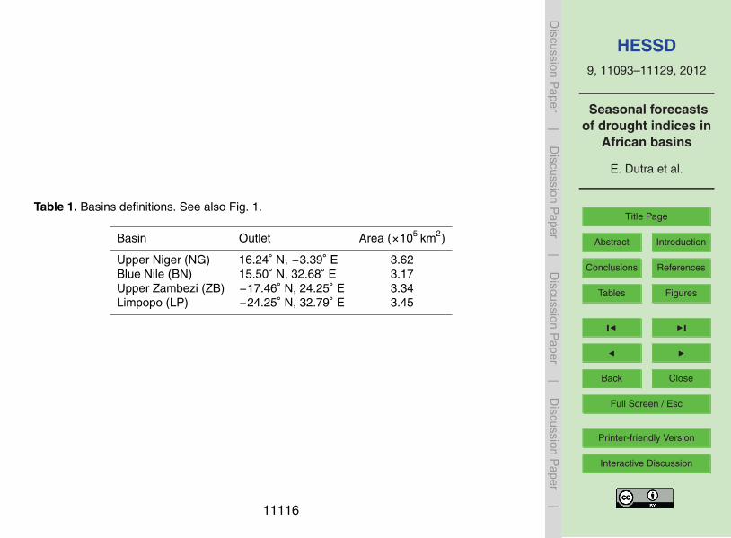
The drought forecasting system was tested in four river basins of the African continent:Blue Nile (NB), Limpopo (LP), Upper Niger (NG) and Zambezi (ZB) (Table 1 and Fig. 1).The catchment definitions were taken from the river network and basins created byYamazaki et al. (2009). The location of the basins was selected to sample differentclimatic regions of Africa, with different precipitation distributions along the year. The10

regions are defined as hydrological basins instead of lat/lon limits since basins havea geographical meaning draining to the same river. All the basins have a similar size(see Table 1) of about 3.5×105 km2, corresponding to approximately 60 grid points ofERAI or S4 and 4.5 grid points of GPCP and CAMS-OPI. The possible ranges of basinssizes are not addressed in this study. This will mainly depend on prior knowledge of15

the region (precipitation patterns and variability), and underlying skill of the seasonalforecasts (avoiding merging region with different skill).Very small basins will not allowfor the spatial filtering that reduces precipitation noise, while very large basins (e.g.entire Nile, Niger) might account for different climatic regions with different forecastskill.20

3 Results

3.1 Quality of observations

Throughout the paper GPCP is assumed to be the ground truth and is used as bench-mark for drought monitoring. However, the quality of this large-scale dataset is signifi-cantly influenced by stations count and changes in the number of stations in time. Since25

11103





HESSD9, 11093–11129, 2012


African basins

E. Dutra et al.

Title Page



Tables Figures

J I

J I

Back Close

Full Screen / Esc



Discussion

Paper

|D

iscussionP

aper|

Discussion

Paper

|D

iscussionP

aper|

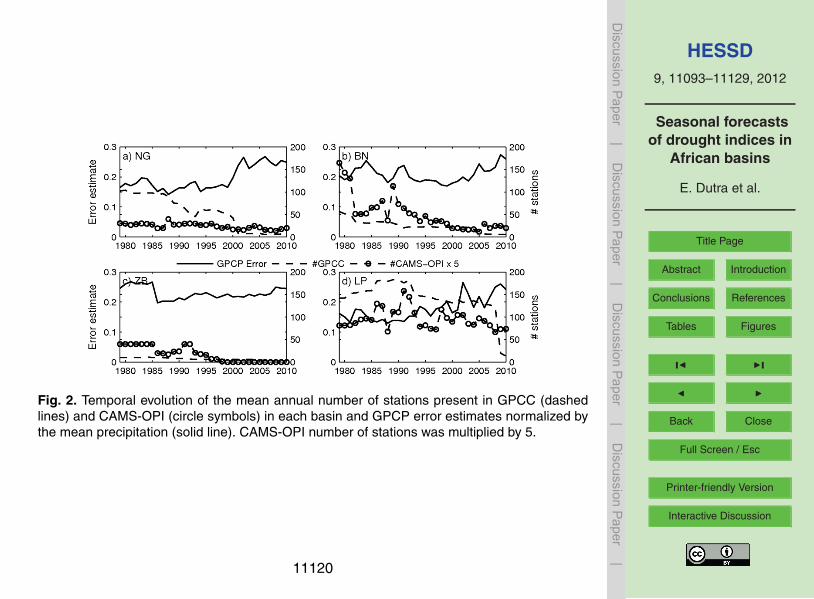
all basin have a similar area (see Table 1), the differences in the stations count and itschange in time can potentially compromise the reliability of GPCP and its temporal ho-mogeneity (essential for drought monitoring). The analysis of the temporal evolution ofthe number of stations present in the Global Precipitation Climatology Centre (GPCC,Rudolf and Schneider, 2005; Schneider et al., 2011), the underlying data used in GPCP5

over land, along with the error estimates provided by GPCP (Fig. 2) provides a qual-itative overview of possible challenges in GPCP over each basins. In the NG there isa significant drop in the stations count from the early 80’s to late 90’s of about 50 % toa very low number of stations during the last decade. This is reflected in an increaseof the error estimates during the last decade. In both BN and ZB basins, the number of10

stations is lower than in NG, being much lower (around 10) in the ZB. LP is the basinwith more and stable number of stations, expect for a drop in the last 5 yr of the dataset.The number of stations present in CAMS-OPI (Fig. 2) is much lower than in GPCP overthe selected basins, especially in NG, NG and ZB. This will impact its potential use ofCAMS-OPI for real time monitoring, that will be addressed in the next section.15

3.2 Drought monitoring

Precipitation over the Niger (NG) and the Blue Nile (BN) is controlled by the south tonorth and back progression of the West Africa Monsoon. Peak rainfall occurs in theboreal summer (June–September, Fig. 3a, b), when the ITCZ moves to its far north-ern limit producing disturbances that are dynamically linked to the African Easterly20

Jet. These are the first cause for the large scale precipitation observed in the regionat the monsoon onset. Westward propagating mesoscale disturbances generate thedominant convective systems. They feed into the large scale disturbance only duringlate boreal summer (when enough moisture is available) changing the rainfall regimefrom frontal precipitation (June–July) to convective (August–September). The Limpopo25

and Zambezi (ZB) river basins are instead located in East Africa and have their peakprecipitation occurring during boreal winter (Fig. 3c, d). The variability is therefore gen-erally out of phase with that in West Africa (i.e. dry (wet) West Africa corresponds to

11104





HESSD9, 11093–11129, 2012


African basins

E. Dutra et al.

Title Page



Tables Figures

J I

J I

Back Close

Full Screen / Esc



Discussion

Paper

|D

iscussionP

aper|

Discussion

Paper

|D

iscussionP

aper|

wet (dry) East Africa). Although wave activity has not been identified, rainfall tends tobe organized into mesoscale convective systems analogous to those in Sahelian WestAfrica.

In the BN and NG basins, the rainy season (June–September) is captured by alldatasets, with an overestimation in the BN by ERAI (Fig. 3b). S4 forecasts overestimate5

precipitation in both BN and NG in the first month of forecasts with a reduction of thepeak rainfall with lead time. This is an example of model drift with lead time, justifyingthe applied bias correction for each calendar month (initial forecast date) and lead time.In the LP and ZB basins all datasets show a reasonable agreement with GPCP, andS4 has a reduced drift in the mean cycle with lead time.10

The temporal correlation of the SPI-3, 6 and 12 months calculated with ERAI, CAMS-OPI and S4 first month of forecasts (S4L0) against the SPI calculated with GPCP(Table 2, and Fig. 4 for the SPI-12 time series) gives an overview of the potential qualityof each dataset for drought monitoring in the regions. Both ERAI and CAMS-OPI havea good agreement with GPCP in LP for the different time-scales, while in the remaining15

three basins the correlations are lower. In the NG and BN, the SPI derived from the firstmonth of forecasts from S4 has a better agreement with GPCP than ERAI or CAMS-OPI, while in ZB all datasets display low correlations (Table 2). It should be noted thatS4L0 has a better intra-seasonal to inter-annual variability of precipitation anomaliesthan ERAI or CAMS-OPI in the NG and BN regions. ERAI overestimates the decrease20

in rainfall in the Central African region which is likely to be associated with a substantialwarm bias in the model due to an underestimation of aerosol optical depth in the region,as well as changes in the data entering the data assimilation system (Dee et al., 2011).This resulted in an unrealistic model drying that penalizes the SPI scores. The poorperformance of CAMS-OPI, when compared with GPCP, in the NG, BN and ZB basins25

is most likely linked with the low number of stations used (Fig. 2), mainly due to thenear real-time restriction, since not all stations report in near real-time.

An independent dataset, the monthly mean anomalies of river discharge, availablefrom the Global Runoff Data Centre (GRDC) were compared with the SPI. The river

11105





HESSD9, 11093–11129, 2012


African basins

E. Dutra et al.

Title Page



Tables Figures

J I

J I

Back Close

Full Screen / Esc



Discussion

Paper

|D

iscussionP

aper|

Discussion

Paper

|D

iscussionP

aper|

discharge accounts for the upstream drainage area that corresponds to the basin defi-nition, and was only available in the Niger (GRDC station Dire, ID: 1134700) and Zam-bezi (GRDC station KATIMA MULILO, ID: 1291100). There is a reasonable agreementbetween the GPCP SPI-12 and river discharge in the NG basin with a temporal correla-tion of 0.65 (Table 3, Fig. 4) while the correlations with the remaining datasets are much5

lower. This can be interpreted as an indirect assessment of the precipitation datasets.In ZB the temporal correlations are lower for GPCP. This could be associated with thereduced number of stations entering GPCP. Even if precipitation would be very closeto reality, timing delays in the river network, interaction with groundwater, among otherprocesses, will introduce non-linear effects in the river discharge making its comparison10

with the SPI difficult. Furthermore, such relation might be only present in a sub-set ofcalendar months/ SPI time scales, as Vicente-Serrano et al. (2012) exemplified for theCongo and Orange river basins when comparing with the Standardized PrecipitationEvapotranspiration Index (SPEI, Vicente-Serrano et al., 2010).

The spatial patterns of the temporal correlations of the SPI-3 and 12 calculated from15

the different products are in agreement with GPCP in Southern and North-West Africa,while in Central Africa (between the 20◦ North/South parallels) ERAI and CAMS-OPIhave low or non-significant correlations, especially for the SPI-12 (Fig. 5). However,CAMS-OPI tends to have a better performance than ERAI. S4L0 has in general a lowervariability than ERAI or CAMS-OPI, except over a latitudinal band South of Sahel (in-20

cluding the NG and BN basins), being a good candidate for drought monitoring in thoseregions, considering the poor performance of ERAI and CAMS-OPI.

3.3 Drought forecasting

The skill of the seasonal forecasts of SPI will depend on the skill of the underlyingseasonal forecasts of precipitation and on the quality of the monitoring (for long SPI25

time scales and short lead times, where the monitoring dominates over the forecast).These two components of the skill can be separately analyzed, by (i) accessing the

11106





HESSD9, 11093–11129, 2012


African basins

E. Dutra et al.

Title Page



Tables Figures

J I

J I

Back Close

Full Screen / Esc



Discussion

Paper

|D

iscussionP

aper|

Discussion

Paper

|D

iscussionP

aper|

skill of the seasonal forecasts of precipitation and (ii) evaluating the potential skill of theSPI seasonal forecast, i.e. using a perfect monitoring product.

3.3.1 Precipitation monitoring skill

Over LP, NG and BN, S4 has skill in first month of forecasts, explaining the good perfor-mance of the SPI calculated using S4L0 when compared with ERAI and CAMS-OPI,5

especially in the NG and BN basins (Fig. 6). This can be primarily attributed to thepredictability coming from the land-atmosphere initial conditions that will dominate thefirst days of the forecast. With increasing lead time, there is a general drop in skill thatis only present in regions/seasons associated with large-scale climate forcings that canbe captured by the coupled atmosphere-ocean modeling system. In both NG and BN,10

S4 has skill up to two/three months lead time for the forecasts valid between June toSeptember, which is also the main rainy season, while in the LP a similar skill withlead time is also found during November to February, also the rainy season. In the ZB,S4 has a reduced skill (only 3 months at 0 lead time), which is also visible in ERAIand CAMS-OPI. However, ZB was also the basin with lower number of rain-gauges15

included in GPCP, therefore being the most uncertain in terms of verification.

3.3.2 Forecast skill of the benchmark

The potential skill of the SPI forecasts was evaluated by merging the S4 precipitationwith GPCP to create a benchmark of the different SPI time-scales for the seasonalforecasts described above. This method isolates the contribution of the seasonal fore-20

casts of precipitation to the SPI skill, avoiding the problems of the different monitoringproducts. On a regional scale, this can be adapted by using local information, such aslong-term rain gauges and/or gridded precipitation datasets. The SPI seasonal fore-casts using GPCP+S4 were benchmarked against forecasts using the same monitor-ing merged with climatological forecasts (CLM) created by randomly sampling different25

15 yr (same ensemble size as S4) of GPCP.

11107





HESSD9, 11093–11129, 2012


African basins

E. Dutra et al.

Title Page



Tables Figures

J I

J I

Back Close

Full Screen / Esc



Discussion

Paper

|D

iscussionP

aper|

Discussion

Paper

|D

iscussionP

aper|

The ACC of the SPI-12 is very close to 1 in all basins for 0 and 1 months lead time(Fig. 7e–h). In this case, the SPI-12 is built from 11 or 10 months of the monitoring and1 or 2 months of the seasonal forecasts for the 0 and 1 months lead time, respectively.For the short lead times, the monitoring dominates the ACC of the SPI-12 which yieldsscores close to 1 since the verification is done against the same dataset used for5

monitoring. In the SPI-3 the ACC for the 0 lead time is already lower than in the SPI-12, and rapidly drops to low values or not significant in regions/periods with low orno precipitation predictability. For long lead times, there is a drop in the SPI-12 skillin particular for the verification in the calendar months after the rainy season. Thisis associated with the different weight of the monitoring and forecast in regions with10

a pronounced annual cycle. The SPI-12 forecasts valid before the rainy season willtend to have a higher skill, since the core precipitation information comes from themonitoring (year before), while the forecasts valid right after the rainy season will relyon the S4 seasonal prediction. The CRPSS identifies the verification months and leadtime where the SPI forecasts using S4 outperform a simple climatological forecast15

(Fig. 7i–p). Those periods are consistent with higher ACC of S4 compared with CLM(with symbols in Fig. 7a–h), and reflect the underlying skill of S4 precipitation (Fig. 6).

The previous skill analysis, based on ACC and CRPSS, considered the full range ofSPI forecasts. For drought detection/early warning, ROC and REL diagrams (amongothers like the Brier Score) are a useful tool, by testing categorical forecasts, i.e. event20

or no event. A drought event is defined as SPI < −1. The ROC diagrams in Fig. 8 of theSPI-3 and SPI-6 represent the skill of using only precipitation forecasts (no monitor-ing), while in the SPI-12 6 months of monitoring are merged with 6 months of seasonalforecasts. The ROC scores of CLM are close to 0.5 (no information) in all basins forthe SPI-3 and SPI-6 at 2 and 5 months lead time, since these are just a random clima-25

tological sampling (Fig. 8). On the other hand, S4 has skill in drought detection in theNG, BN and LP, and no skill in ZB. For the SPI-12 at 5 months lead time, the ROC ofCLM is always around 0.8 and are outperform by S4 in the NG, BN and LP.

11108





HESSD9, 11093–11129, 2012


African basins

E. Dutra et al.

Title Page



Tables Figures

J I

J I

Back Close

Full Screen / Esc



Discussion

Paper

|D

iscussionP

aper|

Discussion

Paper

|D

iscussionP

aper|

The reliability diagrams (Fig. 9) further support the previous results showing that SPI-3 and SPI-6 with 2 and 5 months lead time, respectively, are reliable in the NG, BN andLP and tend to be over-confident (reliability curves with a slope <1; Fig. 9). While theACC and ROC evaluation indicated a clear difference between S4 and CLM forecastsfor the SPI-12 at 5 months lead time, the reliability diagrams show similar results, with5

slopes of the reliability curves close to 1 with S4 being under-confident (slopes >1)in the BN and LP. The variation of ROC and ROC skill score (ROCSS) with lead timeresume the above results (Fig. 10): (i) in the ZB S4 is similar to a climatological forecast,i.e. no skill, while it outperforms CLM in the NG, BN and LP; (ii) in the SPI-3 the 2months lead time (using the first 3 months of the seasonal forecast) and in the SPI-10

6 the 5 months lead time (using the first 6 months of the seasonal forecast) has thehighest skill scores; (iii) the skill score of the SPI-12 is reduced, i.e. it is difficult to beata climatology based forecast for long SPI time scales, where the monitoring dominates;and (iv) SPI S4 forecasts are never worst than CLM, and their skill are only driven bythe accumulated skill of the S4 precipitation forecasts.15

3.3.3 Seasonal forecast skill

The potential skill allows a clear understanding of the importance and impact of theskill of S4 precipitation, but for a near real-time operational implementation GPCP isnot available. Therefore, a similar analysis to the previous section was performed usingother precipitation products that have long-term records and are available in near real-20

time to assess the actual predictive skill of the merged forecast.The ROC scores for the near real-time forecasts are equal from 2 months lead time

onwards for the SPI-3, and for the 5 months lead time in the SPI-6 since these do notinclude precipitation from the monitoring (Figs. 10 and 11). In the NG and BN ERAIand S4L0 were similar, outperforming CAMS-OPI however having a similar skill with25

0 months lead time to using GPCP as monitoring at 2 months lead time. This meansthat the problems identified in those datasets (Sect. 3.2) leads to a reduction of skill of2 months in the NG and BN and 1 month in LP for the SPI-3. For the SPI-6 the skill

11109





HESSD9, 11093–11129, 2012


African basins

E. Dutra et al.

Title Page



Tables Figures

J I

J I

Back Close

Full Screen / Esc



Discussion

Paper

|D

iscussionP

aper|

Discussion

Paper

|D

iscussionP

aper|

reduction is between 3 to 4 months, while for the SPI-12 only CAMS-OPI is able toreach similar skill to GPCP at 5 months lead time in the LP basin. These results high-light the role of the precipitation monitoring quality for SPI seasonal forecasts, showingthat significant gains in skill can be obtained by using good quality observation/modeledprecipitation.5

4 Conclusions

In this paper the use of different observational (GPCP and CAMS-OPI) and reanalysisdatasets (ERA-Interim) were evaluated concerning their value as monitoring tools fordroughts in four African basins. Furthermore, the skill of the new seasonal forecast(S4) was tested in its ability to forecast droughts on a seasonal scale, in combination10

with reanalysis/observations as well as a stand-alone tool.There is a clear difference in skill of monitoring precipitation anomalies, and thereby

also droughts, depending on the region. In general, monitoring is difficult in the tropicalconvergence zone, and the different datasets show the highest divergence in theseregions. It is therefore important to carefully assess the performance of the monitor-15

ing dataset for the specific region of interest. GPCP shows the highest correlation onlonger time-scales with normalized river discharge in the Niger and Zambezi basinsalthough the low number of stations used and its change over time. However, GPCPis discontinued and cannot serve as a near real-time monitoring tool in the future, butserve as a benchmark observational tool. In this study it was also used to bias-correct20

the reanalysis data. The main conclusions from the monitoring component are:

– drought monitoring in Africa with ERA-Interim is mainly possible outside the trop-ical region;

– the usefulness of near real-time monitoring tools has to be carefully selected de-pending on region;25

11110





HESSD9, 11093–11129, 2012


African basins

E. Dutra et al.

Title Page



Tables Figures

J I

J I

Back Close

Full Screen / Esc



Discussion

Paper

|D

iscussionP

aper|

Discussion

Paper

|D

iscussionP

aper|

– in regions where no reliable near real-time data is available (in this study Niger,Blue Nile and Zambezi) it is better to use just the first month of the seasonalforecasts for drought monitoring.

The new ECMWF seasonal forecast system 4 shows skill as a forecasting tool in mostbasins, and is in no basin performing worse than climate. However at longer time5

scales, where a merge with observational datasets are needed, the selection of thebest observation dataset is paramount. The main conclusions of the drought forecast-ing system applied to the Africa basins are:

– The system 4 seasonal forecast has predictive skill in comparison with climatologyin the Niger, Blue Nile and Limpopo and no skill in the Zambezi basin;10

– Poor quality monitoring products can reduce the potential skill of SPI seasonalforecasts with 2 to 4 months lead time.

The methodology presented in the paper to merge a monitoring and seasonal fore-casts of precipitation in a regional-scale can be adapted by using other sources ofprecipitation for the monitoring (e.g. in-situ rain gauges, gridded precipitation datasets,15

remote sensing estimates) and seasonal forecasts (e.g. other systems, multi-model ap-proaches, statistical methods). This methodology can be also applied on a grid-pointbasis, following downscaling methods as proposed by Yoon et al. (2012), but care hasto be taken when interpreting how seasonal scale predictions of precipitation can bereliable on local scales. Furthermore, the role, quality and skill of other drought indica-20

tors (e.g. based on soil moisture, river discharge, evaporation) has to be established,but such work will be highly dependent on reliable monitoring networks.

Acknowledgements. River discharge observations were provided by the Global Runoff DataCentre (GRDC). This work was funded by the FP7 EU projects DEWFORA http://www.dewfora.net and GLOWASIS (http://www.glowasis.eu).25

11111





http://www.dewfora.net



http://www.glowasis.eu

HESSD9, 11093–11129, 2012


African basins

E. Dutra et al.

Title Page



Tables Figures

J I

J I

Back Close

Full Screen / Esc



Discussion

Paper

|D

iscussionP

aper|

Discussion

Paper

|D

iscussionP

aper|

References

Agustı-Panareda, A., Balsamo, G., and Beljaars, A.: Impact of improved soil moisture onthe ECMWF precipitation forecast in West Africa, Geophys. Res. Lett., 37, L20808,doi:10.1029/2010gl044748, 2010.

Dee, D. P., Uppala, S. M., Simmons, A. J., Berrisford, P., Poli, P., Kobayashi, S., Andrae, U.,5

Balmaseda, M. A., Balsamo, G., Bauer, P., Bechtold, P., Beljaars, A. C. M., van de Berg, L.,Bidlot, J., Bormann, N., Delsol, C., Dragani, R., Fuentes, M., Geer, A. J., Haimberger, L.,Healy, S. B., Hersbach, H., Holm, E. V., Isaksen, L., Kallberg, P., Kohler, M., Matricardi, M.,McNally, A. P., Monge-Sanz, B. M., Morcrette, J. J., Park, B. K., Peubey, C., de Ros-nay, P., Tavolato, C., Thepaut, J. N., and Vitart, F.: The ERA-Interim reanalysis: configuration10

and performance of the data assimilation system, Q. J. Roy. Meteor. Soc., 137, 553–597,doi:10.1002/qj.828, 2011.

Di Giuseppe, F., Molteni, F., and Tompkins, A. M.: A rainfall calibration methodology for impactsmodelling based on spatial mapping, Q. J. Roy. Meteor. Soc., in press, 2012

Dutra, E., Magnunson, L., Wetterhall, F., Cloke, H. L., Balsamo, G., Boussetta, S., and Pappen-15

berger, F.: The 2010–11 drought in the Horn of Africa in the ECMWF reanalysis and seasonalforecast products, Int. J. Climatol., online first: doi:10.1002/joc.3545, 2012.

Greenwood, J. A. and Durand, D.: Aids for Fitting the Gamma Distribution by Maximum Likeli-hood, Technometrics, 2, 55–56, 1960.

Hamill, T. M.: Reliability diagrams for multicategory probabilistic forecasts, Weather Forecast.,20

12, 736–741, doi:10.1175/1520-0434(1997)012<0736:rdfmpf>2.0.co;2, 1997.Hersbach, H.: Decomposition of the continuous ranked probability score for en-

semble prediction systems, Weather Forecast., 15, 559–570, doi:10.1175/1520-0434(2000)015<0559:dotcrp>2.0.co;2, 2000.

Huffman, G. J., Bolvin, D. T., and Adler, R. F.: GPCP Version 2.2 Combined Precipitation25

Data set, WDC-A, NCDC, Asheville, NC., available at: http://www.ncdc.noaa.gov/oa/wmo/wdcamet-ncdc.html (last access: September 2012), 2011.

Ingram, K. T., Roncoli, M. C., and Kirshen, P. H.: Opportunities and constraints for farmers ofWest Africa to use seasonal precipitation forecasts with Burkina Faso as a case study, Agr.Syst., 74, 331–349, 2002.30

IWMI: Managing water for rainfed agriculture, International Water Management Institute WaterIssue Brief, 10, 4 pp., doi:10.5337/2010.223, 2010.

11112





http://dx.doi.org/10.1029/2010gl044748

http://dx.doi.org/10.1002/qj.828

http://dx.doi.org/10.1002/joc.3545

http://dx.doi.org/10.1175/1520-0434(1997)012<0736:rdfmpf>2.0.co;2

http://dx.doi.org/10.1175/1520-0434(2000)015<0559:dotcrp>2.0.co;2



http://www.ncdc.noaa.gov/oa/wmo/wdcamet-ncdc.html



http://dx.doi.org/10.5337/2010.223

HESSD9, 11093–11129, 2012


African basins

E. Dutra et al.

Title Page



Tables Figures

J I

J I

Back Close

Full Screen / Esc



Discussion

Paper

|D

iscussionP

aper|

Discussion

Paper

|D

iscussionP

aper|

Janowiak, J. E. and Xie, P.: CAMS-OPI: a global satellite-rain gauge merged product for real-time precipitation monitoring applications, J. Climate, 12, 3335–3342, doi:10.1175/1520-0442(1999)012<3335:coagsr>2.0.co;2, 1999.

Jones, J. W., Hansen, J. W., Royce, F. S., and Messina, C. D.: Potential benefits of climateforecasting to agriculture, Agr. Ecosyst. Environ., 82, 169–184, 2000.5

Keyantash, J. and Dracup, J. A.: The quantification of drought: An evaluation of drought indices,B. Am. Meteorol. Soc., 83, 1167–1180, 2002.

Lamb, P. J., Timmer, R. P., and Lele, M. I.: Professional development for providers of seasonalclimate prediction, Clim. Res., 47, 57–75, doi:10.3354/cr00949, 2011

Lander, J. and Hoskins, B. J.: Believable Scales and Parameterizations in a Spec-10

tral Transform Model, Mon. Weather Rev., 125, 292–303, doi:10.1175/1520-0493(1997)125<0292:bsapia>2.0.co;2, 1997.

Lloyd-Hughes, B. and Saunders, M. A.: A drought climatology for Europe, Int. J. Climatol., 22,1571–1592, 2002.

Mason, S. J. and Graham, N. E.: Conditional probabilities, relative operating characteris-15

tics, and relative operating levels, Weather Forecast., 14, 713–725, doi:10.1175/1520-0434(1999)014<0713:cproca>2.0.co;2, 1999.

McKee, T. B. N., Doesken, J., and Kleist, J.: The relationship of drought frecuency and durationto time scales, Eight Conf. On Applied Climatology, Anaheim, CA, Am. Meteorol. Soc., 179–184, 1993.20

Millner, A. and Washington, R.: What determines perceived value of seasonal climate fore-casts? A theoretical analysis, Global Environ. Change, 21, 209–218, 2011.

Molteni, F., Stockdale, T., Balmaseda, M., BALSAMO, G., Buizza, R., Ferranti, L., Magnun-son, L., Mogensen, K., Palmer, T., and Vitart, F.: The new ECMWF seasonal forecast system(system 4), ECMWF Tech. Memo., 656, 49 pp., 2011.25

Nicholson, S. E., Tucker, C. J., and Ba, M. B.: Desertification, drought, and surface veg-etation: an example from the West African Sahel, B. Am. Meteorol. Soc., 79, 815–829,doi:10.1175/1520-0477(1998)079<0815:ddasva>2.0.co;2, 1998.

Rudolf, B. and Schneider, U.: Calculation of gridded precipitation data for the global land-surface using in-situ gauge observations, in: Proceeding of the 2nd Workshop of the In-30

ternational Precipitation Working Group IPWF, Monterey, October 2004, EUMETSAT, ISBN92-9110-070-6, ISSN 1727-432X, 231–247, 2005.

11113





http://dx.doi.org/10.1175/1520-0442(1999)012<3335:coagsr>2.0.co;2



http://dx.doi.org/10.3354/cr00949

http://dx.doi.org/10.1175/1520-0493(1997)125<0292:bsapia>2.0.co;2



http://dx.doi.org/10.1175/1520-0434(1999)014<0713:cproca>2.0.co;2



http://dx.doi.org/10.1175/1520-0477(1998)079<0815:ddasva>2.0.co;2

HESSD9, 11093–11129, 2012


African basins

E. Dutra et al.

Title Page



Tables Figures

J I

J I

Back Close

Full Screen / Esc



Discussion

Paper

|D

iscussionP

aper|

Discussion

Paper

|D

iscussionP

aper|

Saha, S., Nadiga, S., Thiaw, C., Wang, J., Wang, W., Zhang, Q., Van den Dool, H. M.,Pan, H. L., Moorthi, S., Behringer, D., Stokes, D., Pena, M., Lord, S., White, G., Ebisuzaki, W.,Peng, P., and Xie, P.: The NCEP climate forecast system, J. Climate, 19, 3483–3517,doi:10.1175/jcli3812.1, 2006.

Schneider, U., Becker, A., Meyer-Christoffer, A., Ziese, M., and Rudolf, B.: Global precipita-5

tion analysis products of the GPC C., Global Climatology Centre (GPCC), DWD, InternetPublikation, 1–13, 2011.

Simmons, A. J. and Hollingsworth, A.: Some aspects of the improvement inskill of numerical weather prediction, Q. J. Roy. Meteor. Soc., 128, 647–677,doi:10.1256/003590002321042135, 2002.10

Sohn, S.-J., Tam, C.-Y., Ashok, K., and Ahn, J.-B.: Quantifying the reliability of precipitationdatasets for monitoring large-scale East Asian precipitation variations, Int. J. Climatol., 32,1520–1526, doi:10.1002/joc.2380, 2011.

Thomson, M. C., Doblas-Reyes, F. J., Mason, S. J., Hagedorn, R., Connor, S. J., Phindela, T.,Morse, A. P., and Palmer, T. N.: Malaria early warnings based on seasonal climate forecasts15

from multi-model ensembles, Nature, 439, 576–579, 2006.Tompkins, A. M. and Feudale, L.: Seasonal ensemble predictions of West African monsoon

precipitation in the ECMWF system 3 with a focus on the AMMA special observing period in2006, Weather Forecast., 25, 768–788, doi:10.1175/2009waf2222236.1, 2009.

Vicente-Serrano, S.: Differences in spatial patterns of drought on different time scales: an anal-20

ysis of the Iberian Peninsula, Water Resour. Manag., 20, 37–60, 2006.Vicente-Serrano, S. M., Begueria, S., and Lopez-Moreno, J. I.: A multiscalar drought index sen-

sitive to global warming: the standardized precipitation evapotranspiration index, J. Climate,23, 1696–1718, doi:10.1175/2009jcli2909.1, 2010.

Vicente-Serrano, S. M., Beguerıa, S., Gimeno, L., Eklundh, L., Giuliani, G., Weston, D., El Ke-25

nawy, A., Lopez-Moreno, J. I., Nieto, R., Ayenew, T., Konte, D., Ardo, J., and Pegram, G. G. S.:Challenges for drought mitigation in Africa: the potential use of geospatial data and droughtinformation systems, Appl. Geogr., 34, 471–486, doi:10.1016/j.apgeog.2012.02.001, 2012.

WMO: Press release, December 2009 No. 872, 2009.Xie, P. and Arkin, P. A.: Global Precipitation: A 17-year monthly analysis based on gauge ob-30

servations, satellite estimates, and numerical model outputs, B. Am. Meteorol. Soc., 78,2539–2558, doi:10.1175/1520-0477(1997)078<2539:gpayma>2.0.co;2, 1997.

11114





http://dx.doi.org/10.1175/jcli3812.1

http://dx.doi.org/10.1256/003590002321042135

http://dx.doi.org/10.1002/joc.2380

http://dx.doi.org/10.1175/2009waf2222236.1

http://dx.doi.org/10.1175/2009jcli2909.1

http://dx.doi.org/10.1016/j.apgeog.2012.02.001

http://dx.doi.org/10.1175/1520-0477(1997)078<2539:gpayma>2.0.co;2

HESSD9, 11093–11129, 2012


African basins

E. Dutra et al.

Title Page



Tables Figures

J I

J I

Back Close

Full Screen / Esc



Discussion

Paper

|D

iscussionP

aper|

Discussion

Paper

|D

iscussionP

aper|

Xie, P. and Arkin, P. A.: Global Monthly Precipitation Estimates from Satellite-Observed Outgoing Longwave Radiation, J. Climate, 11, 137–164, doi:10.1175/1520-0442(1998)011<0137:gmpefs>2.0.co;2, 1998

Yamazaki, D., Oki, T., and Kanae, S.: Deriving a global river network map and its sub-gridtopographic characteristics from a fine-resolution flow direction map, Hydrol. Earth Syst. Sci.,5

13, 2241–2251, doi:10.5194/hess-13-2241-2009, 2009.Yoon, J.-H., Mo, K., and Wood, E. F.: Dynamic-model-based seasonal prediction of mete-

orological drought over the contiguous United States, J. Hydrometeorol., 13, 463–482,doi:10.1175/jhm-d-11-038.1, 2012.

11115





http://dx.doi.org/10.1175/1520-0442(1998)011<0137:gmpefs>2.0.co;2



http://dx.doi.org/10.5194/hess-13-2241-2009

http://dx.doi.org/10.1175/jhm-d-11-038.1

HESSD9, 11093–11129, 2012


African basins

E. Dutra et al.

Title Page



Tables Figures

J I

J I

Back Close

Full Screen / Esc



Discussion

Paper

|D

iscussionP

aper|

Discussion

Paper

|D

iscussionP

aper|

Table 1. Basins definitions. See also Fig. 1.

Basin Outlet Area (×105 km2)

Upper Niger (NG) 16.24◦ N, −3.39◦ E 3.62Blue Nile (BN) 15.50◦ N, 32.68◦ E 3.17Upper Zambezi (ZB) −17.46◦ N, 24.25◦ E 3.34Limpopo (LP) −24.25◦ N, 32.79◦ E 3.45

11116





HESSD9, 11093–11129, 2012


African basins

E. Dutra et al.

Title Page



Tables Figures

J I

J I

Back Close

Full Screen / Esc



Discussion

Paper

|D

iscussionP

aper|

Discussion

Paper

|D

iscussionP

aper|

Table 2. Temporal correlation of the 3, 6 and 12-month SPI from between GPCP and ERAI,CAMS-OPI and S4L0 (each column) for the different basins.

ERAI CAMS-OPI S4L0

3 6 12 3 6 12 3 6 12

NG 0.60 0.48 0.34 0.49 0.36 0.22 0.57 0.54 0.56BN 0.57 0.50 0.41 0.62 0.54 0.41 0.65 0.68 0.70ZB 0.47 0.47 0.48 0.42 0.48 0.47 0.37 0.42 0.39LP 0.83 0.86 0.90 0.87 0.89 0.89 0.53 0.59 0.68

11117





HESSD9, 11093–11129, 2012


African basins

E. Dutra et al.

Title Page



Tables Figures

J I

J I

Back Close

Full Screen / Esc



Discussion

Paper

|D

iscussionP

aper|

Discussion

Paper

|D

iscussionP

aper|

Table 3. Temporal correlation of the 12-month SPI from ERAI, CAMS-OPI, S4 and GPCP withthe normalized monthly discharge in the NG and ZB basins.

ERAI CAMS-OPI S4L0 GPCP

NG 0.36 0.27 0.49 0.65ZB 0.45 0.46 0.37 0.54

11118





HESSD9, 11093–11129, 2012


African basins

E. Dutra et al.

Title Page



Tables Figures

J I

J I

Back Close

Full Screen / Esc



Discussion

Paper

|D

iscussionP

aper|

Discussion

Paper

|D

iscussionP

aper|

23

581

Figure 1. Basins definition (dark gray), and the full basin (dark and light gray). See also table 582

1. 583

584

Fig. 1. Basins definition (dark gray), and the full basin (dark and light gray). See also Table 1.

11119





HESSD9, 11093–11129, 2012


African basins

E. Dutra et al.

Title Page



Tables Figures

J I

J I

Back Close

Full Screen / Esc



Discussion

Paper

|D

iscussionP

aper|

Discussion

Paper

|D

iscussionP

aper|

24

585

Figure 2. Temporal evolution of the mean annual number of stations present in GPCC 586

(dashed lines) and CAMS-OPI (circle symbols) in each basin and GPCP error estimates 587

normalized by the mean precipitation (solid line). CAMS-OPI number of stations was 588

multiplied by 5. 589

590

Fig. 2. Temporal evolution of the mean annual number of stations present in GPCC (dashedlines) and CAMS-OPI (circle symbols) in each basin and GPCP error estimates normalized bythe mean precipitation (solid line). CAMS-OPI number of stations was multiplied by 5.

11120





HESSD9, 11093–11129, 2012


African basins

E. Dutra et al.

Title Page



Tables Figures

J I

J I

Back Close

Full Screen / Esc



Discussion

Paper

|D

iscussionP

aper|

Discussion

Paper

|D

iscussionP

aper|

25

591

Figure 3. Mean annual cycle of precipitation over the selected basins. The shaded area 592

represents the range (+/- 1 standard deviation) of observed (GPCP-red) and modeled (S4, 593

gray) precipitation in the hindcast period (1981-2010), comparing with ERAI (blue), CAMS-594

OPI (green). The time series for the seasonal forecasts uses the first (S4-L0,thick black) and 595

last (S4-L6, tick gray) month of forecasts and the 15 ensemble members. 596

Fig. 3. Mean annual cycle of precipitation over the selected basins. The shaded area representsthe range (±1 standard deviation) of observed (GPCP-red) and modeled (S4, gray) precipitationin the hindcast period (1981–2010), comparing with ERAI (blue), CAMS-OPI (green). The timeseries for the seasonal forecasts uses the first (S4-L0,thick black) and last (S4-L6, tick gray)month of forecasts and the 15 ensemble members.

11121





HESSD9, 11093–11129, 2012


African basins

E. Dutra et al.

Title Page



Tables Figures

J I

J I

Back Close

Full Screen / Esc



Discussion

Paper

|D

iscussionP

aper|

Discussion

Paper

|D

iscussionP

aper|

26

597

Figure 4. Evolution of the 12-month SPI in the different basins given by S4 (first forecast 598

month), CAMS-OPI, GPCP and ERAI precipitation, and normalized monthly discharge. The 599

horizontal ticks represent January of each year. In the discharge rows, the symbols identify 600

missing data. 601

Fig. 4. Evolution of the 12-month SPI in the different basins given by S4 (first forecast month),CAMS-OPI, GPCP and ERAI precipitation, and normalized monthly discharge. The horizontalticks represent January of each year. In the discharge rows, the symbols identify missing data.

11122





HESSD9, 11093–11129, 2012


African basins

E. Dutra et al.

Title Page



Tables Figures

J I

J I

Back Close

Full Screen / Esc



Discussion

Paper

|D

iscussionP

aper|

Discussion

Paper

|D

iscussionP

aper|

27

602

Figure 5. Temporal correlation of (a-c) 3-month and (d-f) 12 month SPI between (a,d) GPCP 603

and ERAI, (b,e) GPCP and CAMS-OPI and (c,f) GPCP and S4. 604

605

Fig. 5. Temporal correlation of (a–c) 3-month and (d–f) 12 month SPI between (a,d) GPCP andERAI, (b,e) GPCP and CAMS-OPI and (c,f) GPCP and S4.

11123





HESSD9, 11093–11129, 2012


African basins

E. Dutra et al.

Title Page



Tables Figures

J I

J I

Back Close

Full Screen / Esc



Discussion

Paper

|D

iscussionP

aper|

Discussion

Paper

|D

iscussionP

aper|

28

606

Figure 6. Anomaly correlation coefficient (ACC) of 3-montlhy mean precipitation as a 607

function of verification season (horizontal axis) and dataset (EI: ERAI, CS: CAMS-OPI) and 608

S4 lead time. For example, the color associated with column OND of line ERAI corresponds 609

to the ACC of ERAI versus GPCP mean Oct-Dec precipitation (over 30 years), while the 610

column OND of line SL4L2 corresponds to the ACC of S4 forecasts initialized in August 611

valid for Oct-Dec (two months lead time) compared with Oct-Dec precipitation of GPCP. 612

Only ACC significant at p<0.05 are displayed. The forecast and ERAI and CAMS-OPI are 613

verified against GPCP for the period 1981 to 2010. 614

Fig. 6. Anomaly correlation coefficient (ACC) of 3-montlhy mean precipitation as a function ofverification season (horizontal axis) and dataset (EI: ERAI, CS: CAMS-OPI) and S4 lead time.For example, the color associated with column OND of line ERAI corresponds to the ACC ofERAI versus GPCP mean October–December precipitation (over 30 yr), while the column ONDof line SL4L2 corresponds to the ACC of S4 forecasts initialized in August valid for October–December (two months lead time) compared with October–December precipitation of GPCP.Only ACC significant at p < 0.05 are displayed. The forecast and ERAI and CAMS-OPI areverified against GPCP for the period 1981 to 2010.

11124





HESSD9, 11093–11129, 2012


African basins

E. Dutra et al.

Title Page



Tables Figures

J I

J I

Back Close

Full Screen / Esc



Discussion

Paper

|D

iscussionP

aper|

Discussion

Paper

|D

iscussionP

aper|

29

615

Figure 7. Anomaly correlation coefficient (ACC) the seasonal forecasts of SPI-3 (a-d), and 616

SPI-12 (e-h) and continuous rank probability skill score (CRPSS) of SPI-3 (i-l) and SPI-12 617

(m-p). In the color matrix, the horizontal axis represents the verification month and the 618

vertical axis the lead time (months). In the ACC S4 forecasts are compared with GPCP, and 619

the white circles indicate that the S4 ACC > CLM ACC by at least 0.05. In the CRPSS panels 620

S4 CRPS is benchmarked against the CPRS of CLM. 621

Fig. 7. Anomaly correlation coefficient (ACC) the seasonal forecasts of SPI-3 (a–d), and SPI-12(e–h) and continuous rank probability skill score (CRPSS) of SPI-3 (i–l) and SPI-12 (m–p). Inthe color matrix, the horizontal axis represents the verification month and the vertical axis thelead time (months). In the ACC S4 forecasts are compared with GPCP, and the white circlesindicate that the S4 ACCß,>CLM ACC by at least 0.05. In the CRPSS panels S4 CRPS isbenchmarked against the CPRS of CLM.

11125





HESSD9, 11093–11129, 2012


African basins

E. Dutra et al.

Title Page



Tables Figures

J I

J I

Back Close

Full Screen / Esc



Discussion

Paper

|D

iscussionP

aper|

Discussion

Paper

|D

iscussionP

aper|

30

622

Figure 8. Relative operating characteristic (ROC) diagram representing false alarm rate 623

versus hit rate for the SPI-3 for 2 months lead time(a-d), the SPI-6 for 5 months lead time (e-624

h) and the SPI-12 for 5 months lead time (i-l), given by S4 (black) and CLM (gray) in the 625

different basins (columns). Calculations based on 20 thresholds (fraction of ensemble 626

members below -1), from 1 (symbols closer to 0,0) to 0 (symbols closer to 1,1). Both S4 and 627

CLM seasonal forecasts were merged with GPCP for the SPI calculation and the forecasts are 628

verified against the SPI calculated with GPCP. ROC values are given in the legend of each 629

panel. 630

Fig. 8. Relative operating characteristic (ROC) diagram representing false alarm rate versushit rate for the SPI-3 for 2 months lead time (a–d), the SPI-6 for 5 months lead time (e–h) andthe SPI-12 for 5 months lead time (i–l), given by S4 (black) and CLM (gray) in the differentbasins (columns). Calculations based on 20 thresholds (fraction of ensemble members below−1), from 1 (symbols closer to 0,0) to 0 (symbols closer to 1, 1). Both S4 and CLM seasonalforecasts were merged with GPCP for the SPI calculation and the forecasts are verified againstthe SPI calculated with GPCP. ROC values are given in the legend of each panel.

11126





HESSD9, 11093–11129, 2012


African basins

E. Dutra et al.

Title Page



Tables Figures

J I

J I

Back Close

Full Screen / Esc



Discussion

Paper

|D

iscussionP

aper|

Discussion

Paper

|D

iscussionP

aper|

31

631

Figure 9. Reliability diagrams (CLM, S4) and frequency histograms (fCLM, fS4) for SPI < -1 632

forecasts produced by S4 (black lines and white bars) and CLM (gray lines and bars). For 633

perfect reliability the curves should fall on top of the dashed diagonal line. The thin solid 634

lines (CLM* and S4*) are the weighted least-squares regression lines of the reliability curves, 635

and the slope of each curve is displayed in each panel. Each panel represents a particular 636

basin (column) and SPI timescale (lines), with the same organization has in Fig. 8. 637

Fig. 9. Reliability diagrams (CLM, S4) and frequency histograms (fCLM, fS4) for SPI <−1forecasts produced by S4 (black lines and white bars) and CLM (gray lines and bars). Forperfect reliability the curves should fall on top of the dashed diagonal line. The thin solid lines(CLM* and S4*) are the weighted least-squares regression lines of the reliability curves, andthe slope of each curve is displayed in each panel. Each panel represents a particular basin(column) and SPI timescale (lines), with the same organization has in Fig. 8.

11127





HESSD9, 11093–11129, 2012


African basins

E. Dutra et al.

Title Page



Tables Figures

J I

J I

Back Close

Full Screen / Esc



Discussion

Paper

|D

iscussionP

aper|

Discussion

Paper

|D

iscussionP

aper|

32

638

Figure 10. Relative operating characteristic (ROC) of the SPI forecasts of S4 (dashed black) 639

and CLM (dashed gray) and ROC skill score (ROCSS-solid black) as a function of lead time 640

for the 3 (square symbols), 6 (triangle symbols) and 12 (circle symbols) SPI time-scale. The 641

horizontal dotted line at 0.5 represents the minimum ROC skill and at 0 the minimum 642

ROCSS skill (i.e. S4 outperforms CLM). 643

Fig. 10. Relative operating characteristic (ROC) of the SPI forecasts of S4 (dashed black) andCLM (dashed gray) and ROC skill score (ROCSS-solid black) as a function of lead time for the3 (square symbols), 6 (triangle symbols) and 12 (circle symbols) SPI time-scale. The horizontaldotted line at 0.5 represents the minimum ROC skill and at 0 the minimum ROCSS skill (i.e. S4outperforms CLM).

11128





HESSD9, 11093–11129, 2012


African basins

E. Dutra et al.

Title Page



Tables Figures

J I

J I

Back Close

Full Screen / Esc



Discussion

Paper

|D

iscussionP

aper|

Discussion

Paper

|D

iscussionP

aper|

33

644

Figure 11. Relative operating characteristic (ROC) of the S4 SPI forecasts as a function of 645

lead time (months) for different time-scales ( lines) and for the four basins (columns). Each 646

panel compares the ROC of S4 forecasts using GPCP (square symbols), CAMS-OPI (triangle 647

up symbols), ERAI (circle symbols) and S4L0 (triangle left symbols) as monitoring. Note 648

that for the SPI-3 all ROC scores are the same from 2 month lead time onwards and for the 649

SPI-6 for the 5 month lead time since in those lead times only S4 precipitation is used. 650

Fig. 11. Relative operating characteristic (ROC) of the S4 SPI forecasts as a function of leadtime (months) for different time-scales (lines) and for the four basins (columns). Each panelcompares the ROC of S4 forecasts using GPCP (square symbols), CAMS-OPI (triangle upsymbols), ERAI (circle symbols) and S4L0 (triangle left symbols) as monitoring. Note that forthe SPI-3 all ROC scores are the same from 2 month lead time onwards and for the SPI-6 forthe 5 month lead time since in those lead times only S4 precipitation is used.

11129





Seasonal forecasts of drought indices in African basins

Documents

Transcript of Seasonal forecasts of drought indices in African basins