To Combine Forecasts or to Combine Information

To Combine Forecasts or to Combine Information?∗

Huiyu Huang†

Department of EconomicsUniversity of California, Riverside

Tae-Hwy Lee‡

Department of EconomicsUniversity of California, Riverside

January 2007

Abstract

When the objective is to forecast a variable of interest but with many explanatory variablesavailable, one could possibly improve the forecast by carefully integrating them. There aregenerally two directions one could proceed: combination of forecasts (CF) or combination ofinformation (CI). CF combines forecasts generated from simple models each incorporating a partof the whole information set, while CI brings the entire information set into one super modelto generate an ultimate forecast. Through analysis and simulation, we show the relative meritsof each, particularly the circumstances where forecast by CF can be superior to forecast by CI,when CI model is correctly specified and when it is misspecified, and shed some light on thesuccess of equally weighted CF. In our empirical application on prediction of monthly, quarterly,and annual equity premium, we compare the CF forecasts (with various weighting schemes) to CIforecasts (with methodology mitigating the problem of parameter proliferation such as principalcomponent approach). We find that CF with (close to) equal weights is generally the best anddominates all CI schemes, while also performing substantially better than the historical mean.

Key Words: Equity premium, Factor models, Forecast combination, Information sets, Principalcomponents, Shrinkage.

JEL Classification: C3, C5, G0.

∗We would like to thank Gloria González-Rivera, Bruce Hansen, Lutz Kilian, Michael McCracken, Aman Ullah, aswell as the participants of the Applied Macro Workshop at Duke University, Forecasting Session at North AmericanES Summer 2006 Meetings, Seminar at UC Riverside, and MEG 2006 Meeting, for helpful discussions and comments.All errors are our own.

†Department of Economics, University of California, Riverside, CA 92521-0427, U.S.A. Fax: +1 (951) 827-5685.Email: [email protected].

‡Corresponding author. Department of Economics, University of California, Riverside, CA 92521-0427, U.S.A.Tel: +1 (951) 827-1509. Fax: +1 (951) 827-5685. Email: [email protected].

1 Introduction

When one wants to predict an economic variable using the information set of many explanatory

variables that have been shown or conjectured to be relevant, one can either use a super model

which combines all the available information sets or use the forecast combination methodology.

It is commonly acknowledged in the literature that the forecast generated by all the information

incorporated in one step (combination of information, or CI) is better than the combination of

forecasts from individual models each incorporating partial information (combination of forecasts,

or CF). For instance, Engle, Granger and Kraft (1984) have commented: “The best forecast is

obtained by combining information sets, not forecasts from information sets. If both models are

known, one should combine the information that goes into the models, not the forecasts that come

out of the models”. Granger (1989), Diebold (1989), Diebold and Pauly (1990), and Hendry and

Clements (2004) have similar arguments. It seems that researchers in this field lean more towards

favoring the CI scheme.

However, as Diebold and Pauly (1990) further point out, “... it must be recognized that in many

forecasting situations, particularly in real time, pooling of information sets is either impossible or

prohibitively costly”. Likewise, when models underlying the forecasts remain partially or completely

unknown (as is usually the case in practice), one would never be perfectly certain about which way

to pursue — to combine forecasts from individual models or to combine entire information directly

into one model. On the other hand, growing amount of literature have empirically demonstrated

the superior performance of forecast combination. For recent work, see Stock and Watson (2004)

and Giacomini and Komunjer (2005).1

The frequently asked questions in the existing literature are: “To combine or not to combine”2

and “how to combine”.3 In this paper, we are interested in: “To combine forecasts or to combine

information”. This is an issue that has been addressed but not yet elaborated much. See Chong

and Hendry (1986), Diebold (1989), Newbold and Harvey (2001). Stock and Watson (2004) and

Clements and Galvao (2005) provide empirical comparisons. To our knowledge, there is no formal

proof in the literature to demonstrate that CI is better than CF. This common “belief” might

1A similar issue is about forecast combination versus forecast encompassing, where the need to combine forecastsarises when one individual forecast fails to encompass the other. See Diebold (1989), Newbold and Harvey (2001),among others.

2See Palm and Zellner (1992), Hibon and Evgeniou (2005).3See, for example, Granger and Ramanathan (1984), Deutsch, Granger, and Teräsvirta (1994), Shen and Huang

(2006), and Hansen (2006). Clemen (1989) and Timmermann (2005) provide excellent surveys on forecast combinationand related issues.

1

be based on the in-sample analysis (as we demonstrate in Section 2). On the contrary, from

out-of-sample analysis, we often find CF performs quite well and sometimes even better than

CI. Many articles typically account for the out-of-sample success of CF over CI by pointing out

various disadvantages CI may possibly possess. For example, (a) In many forecasting situations,

particularly in real time, CI by pooling all information sets is either impossible or too expensive

(Diebold 1989, Diebold and Pauly 1990, Timmermann 2005); (b) In a data rich environment

where there are many relevant input variables available, the super CI model may suffer from

the well-known problem of curse of dimensionality (Timmermann 2005); (c) Under the presence

of complicated dynamics and nonlinearity, constructing a super model using CI may be likely

misspecified (Hendry and Clements 2004).

In this paper, we first demonstrate that CI is indeed better than CF in terms of in-sample fit as

maybe commonly believed. Next, we show, for out-of-sample forecasting, CI can be beaten by CF

under certain circumstances even when CI model is the DGP and also when it is misspecified. We

also shed some light on the virtue of equally weighted CF. Then, Monte Carlo study is presented to

illustrate the analytical results. Finally, as an empirical application, we study the equity premium

prediction for which we compare various schemes of CF and CI. Goyal and Welch (2004) explore the

out-of-sample performance of many stock market valuation ratios, interest rates and consumption-

based macroeconomic ratios toward predicting the equity premium. They find that not a single one

would have helped a real-world investor outpredict the then-prevailing historical mean of the equity

premium while pooling all by simple OLS regression performs even worse, and then conclude that

“the equity premium has not been predictable”. We bring CF methodology into predicting equity

premium and compare with CI. To possibly achieve a better performance of CF, we implement CF

with various weighting methods, including simple average, regression based approach (see Granger

and Ramanathan, 1984), and principal component forecast combination (see Stock and Watson,

2004). To mitigate the problem of parameter proliferation in CI, we adopt the factor model with

principal component approach as implemented in Stock and Watson (1999, 2002a,b, 2004, 2005).

We investigate these issues under the theme of comparing CI with CF. We find that CF with

(close to) equal weights is generally the best and dominates all CI schemes, while also performing

substantially better than the historical mean.

The paper is organized as follows. Section 2 shows that the in-sample fit by CI is indeed

superior to that by CF. Section 3 examines analytically the out-of-sample relative merits of CF

in comparison with CI. Section 4 includes some Monte Carlo experiments to compare CI with

2

CF. Section 5 presents an empirical application for equity premium prediction to compare the

performance of various CF and CI schemes. Section 6 concludes.

2 In-sample Fit: CI is Better Than CF

Suppose we forecast a scalar variable yt+1 using the information set available up to time t, It =

xsts=0, where xs is a 1×k vector of weakly stationary variables. Let xs = (x1s x2s) be a non-empty

partition. The CF forecasting scheme poses a set of dynamic regression models

yt+1 = x1tβ1 + 1,t+1, (1)

yt+1 = x2tβ2 + 2,t+1. (2)

The CI takes a model4

yt+1 = x1tα1 + x2tα2 + et+1. (3)

Let Y = (y1 y2 · · · yT )0, Xi = (x0i0 x

0i1 · · · x0i,T−1)0, and i ≡ ( i,1 i,2 . . . i,T )

0 (i = 1, 2).

Note that two individual models (1) and (2) can be equivalently written into two restricted

regressions:

Y = X1α1 +X2α2 + 1, with α2 = 0 (4)

Y = X1α1 +X2α2 + 2, with α1 = 0 (5)

where X1 is T × k1, X2 is T × k2, and X = (X1 X2) is T × k with k = k1 + k2. The CI model

becomes the unrestricted regression:

Y = X1α1 +X2α2 + e ≡ Xα+ e, (6)

where e = (e1 e2 · · · eT )0 and α = (α01 α02)0. Denote the CI fitted value by Y CI ≡ Xα, where

α is the unrestricted OLS estimate for α. Denote the CF fit by Y CF ≡ w1Xα1 + w2Xα2 where

αi (i = 1, 2) (k × 1 vector) are the restricted OLS estimates for the parameters in model (4) and

(5) respectively and wi (i = 1, 2) denote the combination weights.

Write the CF fit as

Y CF ≡ w1Xα1 + w2Xα2 = X(w1α1 + w2α

2) ≡ Xγ,

4Hendry and Clements (2004) have the similar set-up (their equations (5) to (7)). Note that they compare CFwith the best individual forecast but here we compare CF with forecast by the CI model (the DGP in Hendryand Clements, 2004). Harvey and Newbold (2005) investigate gains from combining the forecasts from DGP andmis-specified models, and Clark and McCracken (2006) examine methods of combining forecasts from nested models,while we consider combining forecasts from non-nested (mis-specified) models and compare with models incorporatingall available information directly (CI).

3

with γ ≡ w1α1 + w2α

2. The squared error loss by CF

(Y − Y CF)0(Y − Y CF) ≡ (Y −Xγ)0(Y −Xγ)

is therefore larger than that by CI

(Y − Y CI)0(Y − Y CI) = (Y −Xα)0(Y −Xα),

because α = argminα(Y − Xα)0(Y − Xα). Hence, CI model generates better in-sample fit in

squared-error loss than CF (as long as γ does not coincide with α).

3 Out-of-sample Forecast: CF May Be Better Than CI

Denote the one-step out-of-sample CI and CF forecasts as

yCIT+1 = xT αT = x1T α1,T + x2T α2,T ,

yCFT+1 = w1y(1)T+1 + w2y

(2)T+1 = w1x1T β1,T + w2x2T β2,T ,

where y(1)T+1 and y(2)T+1 are forecasts generated by forecasting models (1) and (2) respectively, and

wi (i = 1, 2) denote the forecast combination weights. All parameters are estimated using strictly

past information (up to time T ) as indicated in subscript. Let eT+1 ≡ yT+1 − yCIT+1 denote the

forecast error by CI, i,T+1 ≡ yT+1 − y(i)T+1 denote the forecast errors by the first (i = 1) and the

second (i = 2) individual forecast, and eCFT+1 ≡ yT+1 − yCFT+1 denote the forecast error by CF.

We consider two cases here, first when the CI model is correctly specified for the DGP and

second when it is not. We show that even in the first case when the CI model coincides with the

DGP, CF can be better than CI in a finite sample. When the CI model is not correctly specified

for the DGP and suffers from omitted variable problem, we show that CF can be better than CI

even in a large sample (T → ∞). Furthermore, we discuss the weighting of CF in the shrinkage

framework as in Diebold and Pauly (1990) and compare with CI.

3.1 When the CI model is correctly specified

Consider predicting yt one-step ahead using information up to time t. Assume et ∼ IID(0, σ2e)

independent of xt−1 in the DGP model (3). Note that the unconditional MSFE by CI forecast is

MSFECI = E[E[e2T+1|IT ]] = E[V arT (yT+1) + [ET (eT+1)]2]

= E(e2T+1) +E[(α− αT )0x0TxT (α− αT )]

= σ2e +E[e0X(X 0X)−1x0TxT (X0X)−1X 0e]

= σ2e + T−1σ2eEtr[x0TxT (T−1X 0X)−1], (7)

4

where V arT (·) and ET (·) denote the conditional variance and the conditional expectation given

information IT up to time T . Given that xt is weakly stationary and T−1X 0X is bounded, the

second term is positive and O(T−1). Similarly,

MSFECF = E[E[(eCFT+1)2|IT ]] = E[V arT (yT+1) + [ET (e

CFT+1)]

2]

= σ2e +E[ET (yT+1 − yCFT+1)]2

= σ2e +E(xTα−2X

i=1

wixiT (X0iXi)

−1X 0iY )

2. (8)

Therefore, it follows that:

Proposition 1. Assume (3) is the DGP model and et ∼ IID(0, σ2e) independent of xt−1. The CF

forecast is better than the CI forecast under the MSFE loss if the following condition holds:

T−1σ2eEtr[x0TxT (T−1X 0X)−1] > E(xTα−2X

i=1

wixiT (X0iXi)

−1X 0iY )

2. (9)

Note that αT → α, a.s. as T → ∞. Therefore, as T → ∞, MSFECI ≤ MSFECF always

follows. For a finite T , however, even when the CI model (3) is the DGP, due to the parameter

estimation error in αT , the squared conditional bias by yCIT+1 can possibly be greater than that

by yCFT+1.5 Under such situation, forecast by CF is superior to forecast by CI in terms of MSFE.

Harvey and Newbold (2005) have the similar finding: forecasts from the true (but estimated) DGP

do not encompass forecasts from competing mis-specified models in general, particularly when T

is small. By comparing the restricted and unrestricted models Clark and McCracken (2006) note

also the finite sample forecast accuracy trade-off resulted from parameter estimation noise in their

simulation and in empirical studies.

The condition (9) in Proposition 1 is more likely to hold when the LHS of (9) is large. This

would happen when: (a) the sample size T is not large; (b) σ2e is big; (c) dimension of xt is large;6

and/or (d) x0its are highly correlated. See Section 4 where these circumstances under which CF

may be better than CI are illustrated by Monte Carlo evidence.

5Note that it is possible to control for the combination weights wi’s to make this condition satisfied. That is, withsuitably chosen combination weights, CF can still beat the DGP model CI. The range for such wi’s may be calibratedby numerical methods. In Section 4 Monte Carlo evidence demonstrates what are such wi’s.

6To see this, note that if xt ∼ INk(0, Ω), then Etr[x0TxT (T−1X0X)−1] ' trΩΩ−1 = k, the dimension of xt.Further, the LHS of condition (9) simplifies into T−1σ2ek, which is well-known.

5

3.2 When the CI model is not correctly specified

Often in real time forecasting, DGP is unknown and the collection of explanatory variables used

to forecast the variable of interest is perhaps just a subset of all relevant ones. This situation

frequently occurs when some of the relevant explanatory variables are simply unobservable. For

instance, in forecasting the output growth, total expenditures on R&D and brand building may

be very relevant predictors but are usually unavailable. They may thus become omitted variables

for predicting output growth. To account for these more practical situations, we now examine the

case when the CI model is misspecified with some relevant variables omitted. In this case, we

demonstrate that CF forecast can be superior to CI forecast even in a large sample. Intuitively,

this is expected to happen likely because when the CI model is also misspecified, the bias-variance

trade-off between large and small models becomes more evident, thus leading to possibly better

chance for CF forecast (generated from a set of small models) to outperform CI forecast (generated

from one large model).

Consider forecasting yT+1 using the CI model (3) and the CF scheme given by (1) and (2)

with the information set (x1s x2s)Ts=0. Suppose, however, that the true DGP involves one more

variable x3t

yt+1 = x1tθ1 + x2tθ2 + x3tθ3 + ηt+1, (10)

where ηt+1 ∼ IID(0, σ2η), is independent of xt = (x1t x2t x3t) (with each xit being 1×ki (i = 1, 2, 3)

and k ≡ k1+k2+k3). The CI model in (3) is misspecified by omitting x3t, the first individual model

in (1) omits x2t and x3t, and the second individual model in (2) omits x1t and x3t. To simplify the

algebra, we assume the conditional mean is zero and consider7

x0t =

⎛⎝ x01tx02tx03t

⎞⎠ ∼ INk

⎡⎣⎛⎝ 000

⎞⎠ ,

⎛⎝ Ω11 Ω12 Ω13Ω21 Ω22 Ω23Ω31 Ω32 Ω33

⎞⎠⎤⎦ . (11)

The forecasts by CI and CF are, respectively, yCIT+1 = x1T α1,T + x2T α2,T , and yCFT+1 = w1y(1)T+1 +

w2y(2)T+1 = w1x1T β1,T + w2x2T β2,T , with wi (i = 1, 2) denoting the forecast combination weights.

Let us consider the special case w1 +w2 = 1 and let w ≡ w1 hereafter. The forecast error by CI is

thus:

eT+1 = yT+1 − yCIT+1 = x1T (θ1 − α1,T ) + x2T (θ2 − α2,T ) + x3T θ3 + eT+1.

7Monte Carlo analysis in Section 4 shows that dynamics in the conditional mean do not affect our general conclu-sions in this section.

6

The forecast errors by the first and the second individual forecast are, respectively:

ˆ1,T+1 = yT+1 − y(1)T+1 = x1T (θ1 − β1,T ) + x2T θ2 + x3T θ3 + eT+1,

ˆ2,T+1 = yT+1 − y(2)T+1 = x1T θ1 + x2T (θ2 − β2,T ) + x3T θ3 + eT+1.

Hence the forecast error by CF is:

eCFT+1 = yT+1 − yCFT+1 = wˆ1,T+1 + (1− w)ˆ2,T+1. (12)

Let zt = (x1t x2t), V ar(zt) = Ωzz, Cov(zt, x3t) = Ωz3, ξ3z,T = x3T−zTΩ−1zz Ωz3, V ar(ξ3z,T ) = Ωξ3z =

Ω33 − Ω3zΩ−1zz Ωz3, θ23 = (θ02 θ03)0, θ13 = (θ01 θ03)0, ξ23.1,T = (x2T − x1TΩ−111 Ω12 x3T − x1TΩ

−111 Ω13),

ξ13.2,T = (x1T − x2TΩ−122 Ω21 x3T − x2TΩ

−122 Ω23), V ar(ξ23.1,T ) = Ωξ23.1 , and V ar(ξ13.2,T ) = Ωξ13.2 .

The following proposition compares CI with CF.

Proposition 2. Assume that (10) is the DGP for yt and (11) holds for xt. The CF forecast is

better than the CI forecast under the MSFE loss if the following condition holds:

θ03Ωξ3zθ3+gCIT > w2θ023Ωξ23.1θ23+(1−w)

2θ013Ωξ13.2θ13+2w(1−w)θ023E[ξ

023.1,T ξ13.2,T ]θ13+g

CFT , (13)

where gCIT = T−1(k1 + k2)σ2η and gCFT = T−1(w2k1 + (1 − w)2k2)σ

2η + 2w(1 − w)E[x1T (β1,T −

E(β1,T ))(β2,T −E(β2,T ))0x02T ] are both O(T−1).

Proof : See Appendix.

Remark 1. The condition (13) that makes CF better than CI can be simplified when T goes

to infinity. Note that it involves both small sample and large sample effect. If we ignore O(T−1)

terms or let T →∞, the condition under which CF is better than CI becomes

θ03Ωξ3zθ3 > w2θ023Ωξ23.1θ23 + (1− w)2θ013Ωξ13.2θ13 + 2w(1− w)θ023E[ξ023.1,T ξ13.2,T ]θ13.

The variance of the disturbance term in the DGP model (10) no long involves since it only appears

in gCIT and gCFT , the two terms capturing small sample effect. Whether this large-sample condition

holds or not is jointly determined by the coefficient parameters in the DGP, θi (i = 1, 2, 3), and the

covariance matrix of xt. We demonstrate the possibilities that CF is better than CI in Section 4

via Monte Carlo simulations, where we investigate both small and large sample effect.

Remark 2. As a by-product, we also note that there is a chance that the CI forecast is even

worse than two individual forecasts. Note that

MSFECI = σ2η + T−1(k1 + k2)σ2η + θ03Ωξ3zθ3,

7

and the MSFE’s by individual forecasts y(1)T+1 and y(2)T+1 are, respectively

MSFE(1) = σ2η + T−1k1σ2η + θ023Ωξ23.1θ23,

MSFE(2) = σ2η + T−1k2σ2η + θ013Ωξ13.2θ13.

SupposeMSFE(1) > MSFE(2), i.e., the second individual forecast is better, then CI will be worse

than the two individual forecasts if

T−1k2σ2η + θ03Ωξ3zθ3 > θ023Ωξ23.1θ23.

This is more likely to happen if the sample size T is not large, and/or σ2η is large. Section 4

illustrates this result via Monte Carlo analysis.

3.3 CI versus CF with specific weights

While the weight w in CF has not yet been specified in the above analysis, we now consider CF

with specific weights. Our aim of this subsection is to illustrate when and how CF with certain

weights can beat CI in out-of-sample forecasting, and shed some light on the success of equally

weighted CF.

Let MSFECI = E(e2T+1) ≡ γ2e, and γ2i ≡ E(ˆ2i,T+1) (i = 1, 2) denote MSFE’s by the two

individual forecasts. Define γ12 ≡ E(ˆ1,T+1ˆ2,T+1). From equation (12), the MSFE of the CF

forecast is

MSFECF = w2γ21 + (1− w)2γ22 + 2w(1− w)γ12 ≡ γ2CF(w). (14)

3.3.1 CI versus CF with optimal weights (CF-Opt)

We consider the “CF-Opt” forecast with weight

w∗ = argminw

γ2CF(w) =γ22 − γ12

γ21 + γ22 − 2γ12, (15)

obtained by solving ∂γ2CF(w)/∂w = 0 (Bates and Granger 1969).8 Denote this CF-Opt forecast as

yCF-OptT+1 = w∗y(1)T+1 + (1− w∗)y(2)T+1, (16)

for which the MSFE is

MSFECF-Opt = E(yT+1 − yCF-OptT+1 )2 =γ21γ

22 − γ212

γ21 + γ22 − 2γ12≡ B

A≡ γ2CF(w

∗),

8Note that if we rearrange terms in (12), it becomes the Bates and Granger (1969) regression

ˆ2,T+1 = w(ˆ2,T+1 − ˆ1,T+1) + eCFT+1,

from which estimate of w∗ is obtained by the least squares.

8

where A ≡ γ21 + γ22 − 2γ12 and B ≡ γ21γ22 − γ212.

First, when MSFECI = γ2e is small, specifically when D ≡ Aγ2e −B < 0 (γ2e < γ2CF(w∗) = B

A ),

we have γ2e < γ2CF(w) for any w. In this case it is impossible to form CF to beat CI. This may

happen when the CI model is correctly specified for the DGP and the sample size T is large as

discussed in Proposition 1, by recalling that when T →∞,

γ2e =MSFECI = σ2e < σ2e +E[ET (eCFT+1)]

2 =MSFECF = γ2CF(w). (17)

Second, when γ2e is large, specifically when D > 0 (γ2e > γ2CF(w∗) = B

A ), we have γ2e > γ2CF(w)

for some w. In this case there exists some w such that CF beats CI. This may happen when the CI

model is correctly specified for the DGP and the sample size T is not large (as shown by Proposition

1) or when the CI model is not correctly specified (as shown by Proposition 2).

Next, consider the case when γ2e = γ2CF(w) for some w. Such w can be obtained by solving the

quadratic equation w2γ21 + (1− w)2γ22 + 2w(1− w)γ12 = γ2e on w, with solutions

wL ≡ (γ22 − γ12)−√D

γ21 + γ22 − 2γ12= w∗ −

√D

A,

wU ≡ (γ22 − γ12) +√D

γ21 + γ22 − 2γ12= w∗ +

√D

A,

where D ≡ (γ21 + γ22 − 2γ12)γ2e − (γ21γ22 − γ212) ≡ Aγ2e −B. Such real-valued wL and wU exist when

D ≥ 0 or, equivalently, when γ2e ≥ BA .

In summary, when D ≥ 0, the interval (wL wU ) is not empty and one can form a CF forecast

that is better than or equal to the CI forecast. This is possible when the MSFE by CI (γ2e) is

relatively large; or when γ12 is highly negative (while assuming others fixed) as in this caseBA

becomes small to make γ2e >BA (D > 0) more likely to hold. In Section 4 we conduct Monte Carlo

simulations to further investigate these possibilities.

3.3.2 CI versus CF with equal weights (CF-Mean)

In light of the frequently discovered success of the simple average for combining forecasts (Stock and

Watson 2004, Timmermann 2005), we now compare the CI forecast with the “CF-Mean” forecast

with weight w = 12 defined as

yCF-MeanT+1 =1

2y(1)T+1 +

1

2y(2)T+1, (18)

for which the MSFE is

MSFECF-Mean = E(yT+1 − yCF-MeanT+1 )2 =1

4(γ21 + γ22 + 2γ12) ≡ γ2CF(

1

2).

9

We note that CF-Opt always assigns a larger (smaller) weight to the better (worse) individual

forecast, since the optimal weight w∗ for the first individual forecast is less than 12 if it is the worse

one (w∗ = γ22−γ12γ21+γ

22−2γ12

< 12 if γ

21 > γ22); and the weight is larger than

12 when it is the better

one (w∗ > 12 if γ

21 < γ22). Also note that w

∗ = 12 if γ

21 = γ22. One practical problem is that w∗

is unobservable. In practice, w∗ may be estimated and the consistently estimated weight w may

converge to w∗ in large sample. When the in-sample estimation size T is large we use CF-Opt

(Bates and Granger 1969, Granger and Ramanathan 1984). However, in small sample when T is

small, the estimated weight w may be in some distance away from w∗, so it may be possible that

w /∈ (wL wU ) while w∗ ∈ (wL wU ). In this case the CF forecast using the estimated weight w will

be worse than the CI forecast. In addition, if CF-Mean is better than CI, it is possible that we

may have the following ranking

γ2CF(w) > γ2e > γ2CF(1

2) ≥ γ2CF(w

∗). (19)

Hence, when the prediction noise is large and T is small, we may be better off by using the CF-

Mean instead of estimating the weights. See Smith and Wallis (2005), where they address the so

called forecast combination puzzle – the simple combinations such as CF-Mean are often found

to outperform sophisticated weighted combinations in empirical applications, by the effect of finite

sample estimation error of the combining weights.

To explore more about weighting in CF, we further consider shrinkage estimators for w. In case

when the above ranking of (19) holds, we can shrink the estimated weight w towards the equal

weight 12 to reduce the MSFE. We have discussed three alternative CF weights: (a) w = w , (b)

w = 12 , and (c) w = w∗. It is likely that w∗ may be different from both w and 1

2 . The relative

performance of CF with w and CF-Mean depends on which of w and 12 is closer to w

∗. Dependent

on the relative distance between w and w∗, between 12 and w

∗, and between w and 12 , the shrinkage

of w towards 12 could work or may not work. The common practice of shrinking w towards12 may

improve the combined forecasts as long as shrinking w towards 12 is also to shrink w towards w∗.

The length of the interval (wL wU ) is 2√D

A where D ≡ Aγ2e−B. Hence the interval that admits CF

over CI becomes larger when D is larger (this happens when γ2e is larger ceteris paribus). As we

will see from the simulation results in Section 4, shrinkage of w towards 12 works quite well when

the noise in the DGP is large (hence γ2e is large) and when the in-sample size T is small. When the

noise is not large or T is large, CI is usually the best when it is correctly specified for the DGP.

However, when CI is not correctly specified for the DGP it can be beaten by CF even in a large

sample. The CF with w (i.e., obtained from the Regression Approach for weights as suggested by

10

Granger and Ramanathan (1984), denoted as CF-RA, and its shrinkage version towards the equal

weights, denoted as CF-RA(κ) (the shrinkage parameter κ will be detailed in Section 4)) generally

works marginally better than CF-Mean. As Diebold and Pauly (1990) point out, CF-RA with

κ = 0 and CF-Mean may be considered as two polar cases of the shrinkage. More shrinkage to the

equal weights is not necessarily better, which can also be observed from the Monte Carlo results in

Section 4.

However, we note that the finite sample estimation error explanation for the success of CF-Mean

(as in Smith and Wallis 2005 and as illustrated above) holds probably only when the unobserv-

able optimal combination weight w∗ is very close to 12 such that CF-Mean is about CF-Opt hence

dominating other sophisticated combinations where estimation errors often involve. It is unlikely

that CF-Mean would outperform other CF with weights obtained by the regression equivalent of

w∗ when w∗ is very close to 1 (or 0). Such values of w∗ happen when the first (second) individual

forecast is clearly better than or encompasses the second (first) individual forecast such that com-

bination of the two has no gains. See Hendry and Clements (2004) for illustrations of situations

where combination forecast gains over individual ones.

Therefore, in order to shed more light on the empirical success of simple average forecast com-

bination, i.e., the CF-Mean, it is worth investigating under what kind of DGP structures and

parameterizations one could have w∗ ' 12 so that CF-Mean ' CF-Opt. We consider again the

DGP (by equations (10) and (11)) discussed in Section 3.2 where CI is misspecified. The DGP in

Section 3.1 where CI model is correctly specified for the DGP is actually a special case of equation

(10) when we let θ3 ≡ 0. First, we note again that w∗ = 12 if γ

21 = γ22. Second, from the discussions

in Section 3.2 we have

γ21 ≡MSFE(1) = σ2η + T−1k1σ2η +

¡θ02 θ

03

¢Ωξ23.1

µθ2θ3

¶,

γ22 ≡MSFE(2) = σ2η + T−1k2σ2η +

¡θ01 θ

03

¢Ωξ13.2

µθ1θ3

¶,

where it is easy to show that

Ωξ23.1 =

µΩ22 − Ω21Ω−111 Ω12 Ω23 − Ω21Ω−111 Ω13Ω32 − Ω31Ω−111 Ω12 Ω33 − Ω31Ω−111 Ω13

¶,

and

Ωξ13.2 =

µΩ11 − Ω12Ω−122 Ω21 Ω13 − Ω12Ω−122 Ω23Ω31 − Ω32Ω−122 Ω21 Ω33 − Ω32Ω−122 Ω23

¶.

Therefore, to make γ21 = γ22 (so that w∗ = 1

2) one sufficient set of conditions is θ1 = θ2 (implying

k1 = k2) and Ωξ23.1 = Ωξ13.2 . The latter happens when Ω11 = Ω22 and Ω13 = Ω23. Intuitively,

11

when the two individual information sets matter about the same in explaining the variable of

interest, their variations (signal strengths) are also about the same, and they correlate with the

omitted information set quite similarly, the resulting forecast performances of the two individual

forecasts are thus about equal. Clark and McCracken (2006) argue that often in practical reality

the predictive content of some variables of interest is quite low. Likewise, the different individual

information sets used to predict such variables of interest are performing quite similarly (bad,

perhaps). Therefore, a simple average combination of those individual forecasts is often desirable

since in such a situation the optimal combination in the sense of Bates and Granger (1969) is

through equal weighting.9. Since first, our main target of this paper is to compare CF with CI not

among CF with different weighting schemes, and second, to match closer with practical situations,

we focus in our Monte Carlo analysis on the designs of DGPs such that the underlying optimal

combination weight w∗ is 12 . In addition, we consider one exceptional case where we let θ1 > θ2 to

make γ21 < γ22 so that w∗ > 1

2 to see how CF with different weights perform in comparison with CI

(other cases such as Ω11 > Ω22 will be similar).

4 Monte Carlo Analysis

In this section we conduct Monte Carlo experiments in the context of Section 3 to illustrate under

what specific situations CF can be better than CI in out-of-sample forecasting. We consider two

cases: when the CI model is correctly specified for the DGP (corresponding to Section 3.1) and

when it is not (corresponding to Section 3.2). We use the following two DGPs:

DGP1: with xt = (x1t x2t), so that the CI model in (3) is correctly specified:

yt+1 = x1tθ1 + x2tθ2 + ηt+1, ηt ∼ N(0, σ2η),

xit = ρixit−1 + vit, vt = (v1t v2t) ∼ N(0,Ω2×2),

DGP2: with xt = (x1t x2t x3t), so that the CI model in (3) is not correctly specified:

yt+1 = x1tθ1 + x2tθ2 + x3tθ3 + ηt+1, ηt ∼ N(0, σ2η),

xit = ρixit−1 + vit, vt = (v1t v2t v3t) ∼ N(0,Ω3×3),

where all vit’s are independent of ηt. The pseudo random samples for t = 1, . . . , R + P + 1 are9 In our empirical study on equity premium prediction in Section 5, we find that CF with (very close to) equal

weights generally performs the best compared to other CF with estimated weights and to about all CI schemes, whichmore-or-less confirms this argument

12

generated andR observations are used for the in-sample parameter estimation (with the fixed rolling

window of size R) and the last P observations are used for pseudo real time out-of-sample forecast

evaluation. We experiment with R = 100, 1000, P = 100, and ση = 2j (j = −2,−1, 0, 1, 2, 3, 4).

The number of Monte Carlo replications is 100. Different specifications for covariance matrix Ω

and coefficient vector θ are used. See Tables 1 and 2.

One of the CF methods we use is the Regression Approach (RA) for combining forecasts as

suggested by Granger and Ramanathan (1984), denoted as CF-RA,

yt+1 = intercept+ w1y(1)t+1 + w2y

(2)t+1 + error, t = T0, . . . , R, (20)

where the pseudo out-of-sample forecast is made for t = T0, . . . , R with T0 the time when the

first pseudo out-of-sample forecast is generated (we choose it at the middle point of each rolling

window). The three versions of the CF-RA methods are considered as in Granger and Ramanathan

(1984), namely, (a) CF-RA1 for the unconstrained regression approach forecast combination, (b)

CF-RA2 for the constrained regression approach forecast combination with zero intercept and the

unit sum of the weights w1 + w2 = 1, and (c) CF-RA3 for the constrained regression approach

forecast combination with zero intercept but without restricting the sum of the weights.

To illustrate more the parameter estimation effect on combination weights, we also consider

CF with shrinkage weights based on CF-RA3. Let CF-RA3(κ) denote the shrinkage forecasts

considered in Stock and Watson (2004, p. 412) with the shrinkage parameter κ controlling for the

amount of shrinkage on CF-RA3 towards the equal weighting (CF-Mean). The shrinkage weight

used is wit = λwit + (1− λ)/N (i = 1, 2) with λ = max0, 1− κN/(t− h− T0 −N), N = 2 (the

number of individual forecasts), and h = 1 (one step ahead forecast).10 For simplicity we consider a

spectrum of different values of κ, that are chosen such that CF-RA3(κ) for the largest chosen value

of κ is closest to CF-Mean. We choose ten different values of κ with equal increment depending on

the in-sample size R as presented in Tables 1 and 2.

Table 1 presents the Monte Carlo results for DGP1, for which we simulate two different cases

with Ω2×2 being diagonal (Panel A) and with Ω2×2 being non-diagonal (Panel B). Table 2 presents

the Monte Carlo results for DGP2, for which the CI model is not correctly specified as it omits

x3t. We simulate four different cases with different values for Ω3×3 and θ where unless specified

otherwise we let θ1 = θ2, Ω11 = Ω22, and Ω13 = Ω23 to make optimal weight w∗ = 12 . The four

cases for Table 2 are presented in Panel A (where x1t and x2t are highly positively correlated with

10Stock and Watson (2005) show the various forecasting methods (such as Bayesian methods, Bagging, etc.) in theshrinkage representations.

13

the omitted variable x3t), in Panel B (where x1t and x2t are highly negatively correlated with the

omitted variable x3t), in Panel C (where everything is the same as in Panel B except with smaller

θ3), and in Panel D (where everything is the same as in Panel B except θ1 = 2θ2 to make w∗ >> 12).

In both Tables 1 and 2, all ρi’s are set at zero as the results are similar for different values of ρi

reflecting dynamics in xit (and thus not reported for space).

First, we observe that results presented in Table 1 and Table 2 share some common features:

MSFE increases with ση (the noise in the DGP), but as ση grows, CF-RA3(κ) and CF-mean be-

come better and better and can beat the CI model (whether correctly specified or not). For smaller

R (= 100), there are more chances for CF to outperform CI given higher parameter estimation

uncertainty in a small sample. Besides, the parameter estimation uncertainty makes the CF-RA2,

which is argued to return asymptotically the optimal combination (Bates and Ganger 1969), per-

forms undesirably. The best shrinkage value varies according to different ση values, while generally

a large amount of shrinkage (large κ) is found to be needed since the optimal combination strategy

(except for Table 2 Panel D case) is about equal weighting. As mentioned in Section 3.3, shrinking

too much to the equal weights is not necessarily good. The Monte Carlo evidence confirms this by

noting that for a fixed value of ση, CF-RA3(κ) with some values of κ is better than CF-Mean, and

shrinking too much beyond that κ value sometimes make it deteriorate its performance.

Second, we notice that results in Table 1 and Table 2 differ in several ways. In Table 1 (when

the CI model is correctly specified for the DGP), for smaller R and when the correlation between

x1t and x2t is high, CF with shrinkage weights can beat CI even when disturbance in DGP (ση) is

relatively small. When R gets larger, however, the advantage of CF vanishes. These Monte Carlo

results are consistent with the analysis in Proposition 1 in Section 3.1, where we show CF may

beat CI only in a finite sample. In contrast, by comparing the four panels in Table 2 (when the CI

model is not correctly specified for the DGP), we find that when x1t and x2t are highly negatively

correlated with the omitted variable x3t and θ3 is relatively large (Panel B), the advantage of CF

(for even small values of ση) does not vanish as R gets larger. Moreover, we observe that even the

individual forecasts can outperform CI in a large sample for large ση under this situation. The

negative correlation of x1t and x2t with the omitted variable x3t, and the large value of θ3 play an

important role for CF to outperform CI in a large sample, which is conformable with the analysis

in Section 3.2 (Proposition 2). In addition, Panel D of Table 2 shows that when x1 contributes

clearly more than x2 in explaining the variable of interest y, the first individual forecast dominates

the second one (making the optimal combination weight w∗ close to 1 hence CF-Mean is clearly

14

not working) when the noise in the DGP is not large. However, when the noise in the DGP is

overwhelmingly large (signal to noise ratio is very low) such that the two individual forecasts are

similarly bad, a close to equal weight is still desirable.

5 Empirical Study: Equity Premium Prediction

In this section we study the relative performance of CI versus CF in predicting equity premium out-

of-sample with many predictors including various financial ratios and interest rates. For a practical

forecasting issue like this, we conjecture that CF scheme should be relatively more advantageous

than CI scheme. Possible reasons are, first, it is very unlikely that the CI model (no matter how

many explanatory variables are used) will coincide with the DGP for equity premium given the

complicated nature of financial markets. Second, we deem that the conditions under which CF is

better than CI as we illustrated in Section 3.2 may easily be satisfied in this empirical application.

We obtained the monthly, quarterly and annual data over the period of 1927 to 2003 from the

homepage of Amit Goyal (http://www.bus.emory.edu/AGoyal/). Our data construction replicates

what Goyal and Welch (2004) did. The equity premium, y, is calculated by the S&P 500 market

return (difference in the log of index values in two consecutive periods) minus the risk free rate

in that period. Our explanatory variable set, x, contains 12 individual variables: dividend price

ratio, dividend yield, earnings price ratio, dividend payout ratio, book-to-market ratio, T-bill rate,

long term yield, long term return, term spread, default yield spread, default return spread and

lag of inflation, as used in Goyal and Welch (2004). Goyal and Welch (2004) explore the out-of-

sample performance of these variables toward predicting the equity premium and find that not a

single one would have helped a real-world investor outpredict the then-prevailing historical mean

of the equity premium while pooling all by simple OLS regression performs even worse, and then

conclude that “the equity premium has not been predictable”. Campbell and Thompson (2005)

argue that once sensible restrictions are imposed on the signs of coefficients and return forecasts,

forecasting variables with significant forecasting power in-sample generally have a better out-of-

sample performance than a forecast based on the historical mean. Lewellen (2004) studies in

particular the predictive power of financial ratios on forecasting aggregate stock returns through

predictive regressions. He finds evidence of predictability by certain ratios over certain sample

periods. In our empirical study, we bring the CF methodology into predicting equity premium

and compare with CI since the analysis in Section 3 demonstrates that CF method indeed has its

merits in out-of-sample forecasting practice. In addition, we investigate this issue of predictability

15

by comparing various CF and CI schemes with the historical mean benchmark over different data

frequencies, sample splits and forecast horizons.

5.1 CI schemes

Two sets of CI schemes are considered. The first is the OLS using directly xt (with dimension

N = 12) as the regressor set while parameter estimate is obtained using strictly past data. The

forecast is constructed as yT+1 = (1 x0T )αT . Let us call this forecasting scheme: CI-Unrestricted.

It is named as “kitchen sink” in Goyal and Welch (2004). The second set of CI schemes aims at the

problem associated with high dimension. It is quite possible to achieve a remarkable improvement

on prediction by reducing dimensionality if one applies a factor model by extracting the Principal

Components (PC) (Stock and Watson 2002a,b, 2004). The procedure is as follows:

xt = ΛFt + vt, (21)

yt+1 = (1 F 0t)γ + ut+1. (22)

In equation (21), by applying the classical principal component methodology, the latent common

factors F = (F1 F2 · · · FT )0 is solved by:

F = XΛ/N (23)

where N is the size of xt, X = (x1 x2 · · · xT )0, and factor loading Λ is set to

√N times the

eigenvectors corresponding to the r largest eigenvalues of X 0X (see, for example, Bai and Ng

2002). Once γT is obtained from (22) by regression of yt on (1 F 0t−1) (t = 1, 2, . . . , T ), the forecast

is constructed as yCI-PCT+1 = (1 F 0T )γT (let us denote this forecasting scheme as CI-PC).

If the true number of factors r is unknown, it can be estimated by minimizing some information

criteria. Bai and Ng (2002) focus on estimation of the factor representation given by equation (21)

and the asymptotic inference for r when N and T go to infinity. Equation (22), however, is more

relevant for forecasting and thus it is our main interest. Moreover, we note that the N in our

empirical study is only 12. Therefore, we use AIC and BIC for which estimated number of factors

k is selected by

min 1≤k≤kmaxICk = ln(SSR(k)/T ) + g(T )k,

where kmax is the hypothesized upper limit chosen by the user (we choose kmax = 12), SSR(k) is

the sum of squared residuals from the forecasting model (22) using k estimated factors, and the

16

penalty function g(T ) = 2/T for AIC and g(T ) = lnT/T for BIC.11 Additionally, we consider fix k

a priori at small value like 1,2,3.

5.2 CF schemes

We consider five sets of CF schemes where individual forecasts are generated by using each element

xit in xt: y(i)T+1 = (1 x0iT )βi,T (i = 1, 2, . . . ,N). The first CF scheme, CF-Mean, is computed as

yCF-MeanT+1 = 1N

PNi=1 y

(i)T+1. Second, CF-Median is to compute the median of the set of individual

forecasts, which may be more robust in the presence of outlier forecasts. These two simple weighting

CF schemes require no estimation in weight parameters. Starting from Granger and Ramanathan

(1984), based on earlier works such as Bates and Granger (1969) and Newbold and Granger (1974),

various feasible optimal combination weights have been suggested, which are static, dynamic, time-

varying, or Bayesian: see Diebold and Lopez (1996). Chan, Stock and Watson (1999) and Stock

and Watson (2004) utilize the principal component approach to exploit the factor structure of a

panel of forecasts to improve upon Granger and Ramanathan (1984) combination regressions. They

show this principal component forecast combination is more successful when there are large number

of individual forecasts to be combined. The procedure is to first extract a small set of principal

components from a (large) set of forecasts and then estimate the (static) combination weights for the

principal components. Deutsch, Granger, and Teräsvirta (1994) extend Granger and Ramanathan

(1984) by allowing dynamics in the weights which are derived from switching regression models or

from smooth transition regression models. Li and Tkacz (2004) introduce a flexible non-parametric

technique for selecting weights in a forecast combination regression. Empirically, Stock and Watson

(2004) consider various CF weighting schemes and find the superiority of simple weighting schemes

over sophisticated ones (such as time-varying parameter combining regressions) for output growth

prediction in a seven-country economic data set.

To explore more information in the data, thirdly, we estimate the combination weights wi by

regression approach (Granger and Ramanathan 1984):

yt+1 = w0 +NXi=1

wiy(i)t+1 + et+1, (24)

and form predictor CF-RA, yCF-RAT+1 = w0 +PN

i=1 wiy(i)T+1. Similarly as in Section 4 Monte Carlo

11 In model selection, it is well known that BIC is consistent in selecting the true model, and AIC is minimax-rate optimal for estimating the regression function. Yang (2005) shows that for any model selection criterion to beconsistent, it must behave suboptimally for estimating the regression function in terms of minimax rate of convergence.Bayesian model averaging cannot be minimax-rate optimal for regression estimation. This explains that the modelselected for in-sample fit and estimation would be different than the model selected for out-of-sample forecasting.

17

analysis, we experiment the three different versions of CF-RA. Fourth, we shrink CF-RA3 towards

equally weighted CF by choosing increasing values of shrinkage parameter κ. Finally, we extract

the principal components from the set of individual forecasts and form predictor that may be called

as CF-PC (combination of forecasts using the weighted principal components): see Chan, Stock

and Watson (1999).12 This is to estimate

yt+1 = b0 +kXi=1

biF(i)t+1 + vt+1, (25)

where (F (1)t+1, . . . , F(k)t+1) denotes the first k principal components of (y

(1)t+1, . . . , y

(N)t+1) for t =

T0, . . . , T .13 The CF-PC forecast is then constructed as yCF-PCT+1 = b0 +Pk

i=1 biF(i)T+1. Chan, Stock

and Watson (1999) choose k = 1 since the factor analytic structure for the set of individual forecasts

they adopt permits one single factor – the conditional mean of the variable to be forecast. Our

specifications for individual forecasts in CF, however, differ from those in Chan, Stock and Watson

(1999) in that individual forecasting models considered here use different and non-overlapping

information sets, not a common total information set (which makes individual forecasts differ

solely from specification error and estimation error) as assumed in Chan, Stock and Watson (1999).

Therefore, we consider k = 1, 2, 3. In addition to that, k is also chosen by the information criteria

AIC or BIC, as discussed in Section 5.1.

5.3 Empirical results

Table 3 presents the out-of-sample performance of each forecasting scheme for equity premium

prediction across different forecast horizons h, different frequencies (monthly, quarterly, and annual

in Panels A1 and A2, B, and C) and different in-sample/out-of-sample splits R and P . Data range

from 1927 to 2003 in monthly, quarterly and annual frequencies. All models are estimated using

OLS over rolling windows of size R. MSFE’s are compared. To compare each model with the

benchmark Historical Mean (HM) we also report its MSFE ratio with respect to HM.

First, similarities are found among Panels A1, A2, B, and C. While not reported for space,

although there are a few cases some individual forecasts return relatively small MSFE ratio, the12Also see Stock and Watson (2004), where it is called Principal Component Forecast Combination. In Aguiar-

Conraria (2003), a similar method is proposed: Principal Components Combination (PCC), where the PrincipalComponents Regression (PCR) is combined with the Forecast Combination approach by using each explanatoryvariable to obtain a forecast for the dependent variable, and then combining the several forecasts using the PCRmethod. This idea, as noted in the paper, follows the spirit of Partial Least Squares in the Chemometrics literaturethus is distinguished from what proposed in Chan, Stock and Watson (1999).13 In computing the out-of-sample equity premium forecasts by rolling window scheme with window size R, we set

T = R and choose T0, the time when the first pseudo out-of-sample forecast is generated, at the middle point of therolling window.

18

performance of individual forecasts is fairly unstable while similarly bad. In contrast, we clearly

observe the genuinely stable and superior performance of CF-Mean and CF with shrinkage weights

(while a large amount of shrinkage is imposed so the weights are close to equal weights), compared

to almost all CI schemes across different frequencies, especially for shorter forecast horizons and

for the forecast periods with earlier starting date. CF-Median also appears to perform quite well.

This more-or-less confirms the discussion in Section 3.3 where we shed light on the reasons for the

success of simple average combination of forecasts.

Second, MSFE ratios of the good models that outperform HM are smaller in Panel B (quarterly

prediction) and Panel C (annual prediction) than in Panels A1 and A2 (monthly predictions). This

indicates that with these good models we can beat HM more easily for quarterly and annual series

than for monthly series.

Third, CF-PC with a fixed number of factors (1 or 2) frequently outperforms HM as well, and

by contrast, the CI schemes rarely beat HM by a considerable margin. Generally BIC performs

better than AIC by selecting a smaller k (the estimated number of factors) but worse than using a

small fixed k (= 1, 2, 3).

Fourth, within each panel, we find that generally it is hard to improve upon HM for more

recent out-of-sample periods (forecasts beginning in 1980) and for longer forecast horizons, since

the MSFE ratios tend to be larger under these situations. It seems that the equity premium

becomes less predictable in recent years than older years.

Fifth, we note that the in-sample size R is smaller for the forecast period starting from the

earlier year. In accordance with the conditions under which CF can be superior to CI as discussed

in Section 3, the smaller in-sample size may partly account for the success of CF-Mean over the

forecast period starting from the earlier year in line of the argument about parameter estimation

uncertainty.

In summary, Table 3 shows that CF-Mean, or CF with shrinkage weights that are very close to

equal weights, are simple but powerful methods to predict the equity premium out-of-sample, in

comparison with the CI schemes and to beat the HM benchmark.

6 Conclusions

In this paper, we show the relative merits of combination of forecasts (CF) compared to combination

of information (CI). In the literature, it is commonly believed that CI is optimal. This belief is valid

for in-sample fit as we illustrate in Section 2. When it comes to out-of-sample forecasting, CI is no

19

longer undefeated. In Section 3, through stylized forecasting regressions we illustrate analytically

the circumstances when the forecast by CF can be superior to the forecast by CI, when CI model is

correctly specified and when it is misspecified. We also shed some light on how CF with (close to)

equal weights may work by noting that, apart from the parameter estimation uncertainty argument

(Smith and Wallis 2005), in practical situations the information sets we selected that are used to

predict the variable of interest are often with about equally low predictive content therefore a simple

average combination is often close to optimal. Our Monte Carlo analysis provides some insights on

the possibility that CF with shrinkage or CF with equal weights can dominate CI even in a large

sample.

In accordance with the analytical findings, our empirical application on the equity premium

prediction confirms the advantage of CF in real time forecasting. We compare CF with various

weighting methods, including simple average, regression based approach with principal component

method (CF-PC), to CI models with principal component approach (CI-PC). We find that CF with

(close to) equal weights dominates about all CI schemes, and also performs substantially better

than the historical mean benchmark model. These empirical results highlight the merits of CF

that we analyzed in Section 3 and they are also consistent with much of literature about CF, for

instance, the empirical findings by Stock and Watson (2004) where CF with various weighting

schemes (including CF-PC) is found favorable when compared to CI-PC.

20

Appendix: Proof of Proposition 2

Define θ12 ≡ (θ01 θ02)0 and δα ≡ αT −E(αT ). Note that

E(αT ) = E[(Σz0tzt)−1Σz0tyt+1] = θ12 +E[(Σz0tzt)

−1Σz0tx3t]θ3 = θ12 +Ω−1zz Ωz3θ3,

and V ar(αT ) = T−1σ2ηΩ−1zz , so δα = αT − θ12 − Ω−1zz Ωz3θ3. Thus, the conditional bias by the CI

forecast is

E(eT+1|IT ) = x1T (θ1 − α1,T ) + x2T (θ2 − α2,T ) + x3T θ3

= zT (θ12 − αT ) + x3T θ3 = zT (−Ω−1zz Ωz3θ3 − δα) + x3T θ3

= −zT δα + ξ3z,T θ3,

where IT denotes the total information up to time T . It follows that

MSFECI = E[V arT (yT+1)] +E[(E(eT+1|IT ))2]

= σ2η +E[(−zT δα + ξ3z,T θ3)(−zT δα + ξ3z,T θ3)0]

= σ2η +E[zTV ar(αT )z0T ] + θ03E[ξ

03z,T ξ3z,T ]θ3

= σ2η + T−1σ2ηE[zTΩ−1zz z

0T ] + θ03Ωξ3zθ3

= σ2η + T−1σ2ηtrΩ−1zz E[z0T zT ]+ θ03Ωξ3zθ3

= σ2η + T−1σ2η(k1 + k2) + θ03Ωξ3zθ3. (26)

Similarly, for the two individual forecasts, define δβi ≡ βi,T −E(βi,T ) (i = 1, 2). Given that

E(β1,T ) = E[(Σx01tx1t)−1Σx01tyt+1]

= θ1 +E[(Σx01tx1t)−1Σx01t(x2tθ2 + x3tθ3)]

= θ1 +Ω−111 (Ω12θ2 +Ω13θ3),

and

E(β2,T ) = θ2 +Ω−122 (Ω21θ1 +Ω23θ3),

the conditional biases by individual forecasts are:

E(ˆ1,T+1|IT ) = x1T (θ1 − β1,T ) + x2T θ2 + x3T θ3 = −x1T δβ1 + ξ23.1,T θ23,

E(ˆ2,T+1|IT ) = x1T θ1 + x2T (θ2 − β2,T ) + x3T θ3 = −x2T δβ2 + ξ13.2,T θ13.

21

Hence, similar to the derivation for MSFECI, it is easy to show that

MSFE(1) = σ2η +E[(−x1T δβ1 + ξ23.1,T θ23)(−x1T δβ1 + ξ23.1,T θ23)0]

= σ2η + T−1σ2ηE[x1TΩ−111 x

01T ] + θ023Ωξ23.1θ23

= σ2η + T−1σ2ηk1 + θ023Ωξ23.1θ23, (27)

and

MSFE(2) = σ2η + T−1σ2ηk2 + θ013Ωξ13.2θ13, (28)

by noting that V ar(βi,T ) = T−1σ2ηΩ−1ii (i = 1, 2).

Using equation (12), the conditional bias by the CF forecast is

E(eCFT+1|IT ) = wE(ˆ1,T+1|IT ) + (1− w)E(ˆ2,T+1|IT ).

It follows that

MSFECF = σ2η +E[(E(eCFT+1|IT ))2]

= σ2η +E[w2(E(ˆ1,T+1|IT ))2 + (1− w)2(E(ˆ2,T+1|IT ))2

+2w(1− w)E(ˆ1,T+1|IT )E(ˆ2,T+1|IT )]

= σ2η + w2[T−1σ2ηk1 + θ023Ωξ23.1θ23] + (1−w)2[T−1σ2ηk2 + θ013Ωξ13.2θ13]

+2w(1− w)E[x1T δβ1δ0β2x02T + θ023ξ

023.1,T ξ13.2,T θ13]

= σ2η + gCFT + w2θ023Ωξ23.1θ23 + (1− w)2θ013Ωξ13.2θ13

+2w(1− w)θ023E[ξ023.1,T ξ13.2,T ]θ13, (29)

where gCFT = T−1(w2k1 + (1− w)2k2)σ2η + 2w(1− w)E[x1T δβ1

δ0β2x02T ].

From comparing equation (26) and (29), the result follows.

22

References

Aguiar-Conraria, L. (2003), “Forecasting in Data-Rich Environments”, Cornell University andMinho University, Portugal.

Bai, J. and Ng, S. (2002), “Determining the Number of Factors in Approximate Factor Models”,Econometrica 70, 191-221.

Bates, J.M. and Granger, C.W.J. (1969), “The Combination of Forecasts”, Operations ResearchQuarterly 20, 451-468.

Campbell, J.Y. and Thompson, S.B. (2005), “Predicting the Equity Premium Out of Sample: CanAnything Beat the Historical Average?” Harvard Institute of Economic Research, DiscussionPaper No. 2084.

Chan, Y.L., Stock, J.H., and Watson, M.W. (1999), “A Dynamic Factor Model Framework forForecast Combination”, Spanish Economic Review 1, 91-121.

Chong, Y.Y. and Hendry, D.F. (1986), “Econometric Evaluation of Linear Macro-Economic Mod-els”, Review of Economics Studies, LIII, 671-690.

Clark, T.E. and McCracken, M.W. (2006), “Combining Forecasts from Nested Models”, FederalReserve Bank of Kansas City.

Clemen, R.T. (1989), “Combining Forecasts: A Review and Annotated Bibliography”, Interna-tional Journal of Forecasting, 5, 559-583.

Clements, M.P. and Galvao, A.B. (2005), “Combining Predictors and Combining Informationin Modelling: Forecasting US Recession Probabilities and Output Growth”, University ofWarwick.

Coulson, N.E. and Robins, R.P. (1993), “Forecast Combination in a Dynamic Setting”, Journalof Forecasting 12, 63-67.

Deutsch, M., Granger, C.W.J., and Teräsvirta, T. (1994), “The Combination of Forecasts UsingChanging Weights”, International Journal of Forecasting 10, 47-57.

Diebold, F.X. (1989), “Forecast Combination and Encompassing: Reconciling Two DivergentLiteratures”, International Journal of Forecasting 5, 589-592.

Diebold, F.X. and Lopez, J.A. (1996), “Forecast Evaluation and Combination”, NBER WorkingPaper, No. 192.

Diebold, F.X. and Pauly, P. (1990), “The Use of Prior Information in Forecast Combination”,International Journal of Forecasting, 6, 503-508.

Engle, R.F., Granger, C.W.J. and Kraft, D.F. (1984), “Combining Competing Forecasts of In-flation Using a Bivariate ARCH Model”, Journal of Economic Dynamics and Control 8,151-165.

Giacomini, R. and Komunjer, I. (2005), “Evaluation and Combination of Conditional QuantileForecasts”, Journal of Business and Economic Statistics 23, 416-431.

Goyal, A. and Welch, I. (2005), “A Comprehensive Look at the Empirical Performance of EquityPremium Prediction”, Emory and Yale.

Granger, C.W.J. (1989), “Invited Review: Combining Forecasts - Twenty years Later”, Journalof Forecasting 8, 167-173.

23

Granger, C.W.J. and Ramanathan, R. (1984), “Improved Methods of Combining Forecasts”,Journal of Forecasting 3, 197-204.

Hansen, B.E. (2006), “Least Squares Forecast Averaging", Department of Economics, Universityof Wisconsin, Madison

Harvey, D.I. and Newbold, P. (2005), “Forecast Encompassing and Parameter Estimation", OxfordBulletin of Economics and Statistics 67, Supplement 0305-9049.

Hendry, D.F. and Clements, M.P. (2004), “Pooling of Forecasts”, Econometrics Journal 7, 1-31.

Hibon, M. and Evgeniou, T. (2005), “To Combine or not to Combine: Selecting among Forecastsand Their Combinations”, International Journal of Forecasting 21, 15-24.

Lewellen, J. (2004), “Predicting Returns with Financial Ratios”, Journal of Financial Economics74, 209-235.

Li, F. and Tkacz, G. (2004), “Combining Forecasts with Nonparametric Kernel Regressions”,Studies in Nonlinear Dynamics and Econometrics 8(4), Article 2.

Newbold, P. and Granger, C.W.J. (1974), “Experience with Forecasting Univariate Time Seriesand the Combination of Forecasts”, Journal of the Royal Statistical Society 137, 131-165.

Newbold, P. and Harvey, D.I. (2001), “Forecast Combination and Encompassing”, in A Companionto Economic Forecasting, Clements, M.P. and Hendry, D.F. (ed.), Blackwell Publishers.

Palm, F.C. and Zellner, A. (1992), “To Combine or not to Combine? Issues of Combining Fore-casts”, Journal of Forecasting 11, 687-701.

Shen, X. and Huang, H.-C. (2006), “Optimal Model Assessment, Selection, and Combination",Journal of the American Statistical Association 101, 554-568.

Smith, J. and Wallis, K.F. (2005), “Combining Point Forecasts: The Simple Average Rules, OK?"University of Warwick.

Stock, J.H. and Watson, M.W. (1999), “Forecasting Inflation”, Journal of Monetary Economics44, 293-335.

Stock, J.H. and Watson, M.W. (2002a), “Macroeconomic Forecasting Using Diffusion Indexes”,Journal of Business and Economic Statistics 20, 147-162.

Stock, J.H. and Watson, M.W. (2002b), “Forecasting Using Principal Components from a LargeNumber of Predictors”, Journal of the American Statistical Association 97, 1167-1179.

Stock, J.H. and Watson, M.W. (2004), “Combination Forecasts of Output Growth in a Seven-Country Data Set”, Journal of Forecasting 23, 405-430.

Stock, J.H. and Watson, M.W. (2005), “An Empirical Comparison of Methods for ForecastingUsing Many Predictors”, Harvard and Princeton.

Timmermann, A. (2005), “Forecast Combinations”, forthcoming in Handbook of Economic Fore-casting, Elliott, G., Granger, C.W.J., and Timmermann, A. (ed.), North Holland.

Yang, Y. (2005), “Can the Strengths of AIC and BIC Be Shared? A Conflict between ModelIdentification and Regression Estimation”, Biometrika 92(4), 937-950.

24

Table 1. Monte Carlo Simulation (When CI model is the DGP) This set of tables presents the performance of each forecasting schemes for predicting yt+1 out-of-sample where yt is by DGP:

yt+1 = xtθ + ηt+1 , ηt ~ N(0, ση2); xit = ρixit-1 + vit, vt ~ N(0, Ω), i=1,2. We report the out-of-sample MSFE of each forecasting scheme where bolded term indicates smaller-than-CI case and the smallest number among them is highlighted.

Panel A. No correlation: ⎟⎟⎠

⎞⎜⎜⎝

⎛==⎟⎟

⎠

⎞⎜⎜⎝

⎛=Ω

5.05.0

;0;1001

θρi

R=100, P=100 MSFE ση =0.25 ση =0.5 ση =1 ση =2 ση =4 ση =8 ση =16

ŷ(1) 0.3244 0.5169 1.2847 4.3146 16.4786 66.7677 260.2036

ŷ(2) 0.3182 0.5037 1.2977 4.2801 16.4518 66.8664 260.5220

CI 0.0649 0.2578 1.0416 4.0865 16.3426 67.1837 262.6703

CF-RA1 0.0728 0.2827 1.1316 4.4324 17.3736 70.0208 271.7653

CF-RA2 0.1900 0.3869 1.1860 4.2472 16.5744 67.9264 264.4291

CF-RA3(κ=0) 0.0758 0.2848 1.1238 4.3396 16.9122 68.1654 264.8655

CF-RA3(κ=1) 0.0756 0.2837 1.1199 4.3242 16.8563 67.9897 264.2168

CF-RA3(κ=3) 0.0764 0.2828 1.1135 4.2953 16.7518 67.6645 263.0250

CF-RA3(κ=5) 0.0790 0.2838 1.1091 4.2691 16.6567 67.3742 261.9742

CF-RA3(κ=7) 0.0834 0.2866 1.1066 4.2455 16.5712 67.1189 261.0642

CF-RA3(κ=9) 0.0895 0.2912 1.1062 4.2246 16.4951 66.8984 260.2952

CF-RA3(κ=11) 0.0974 0.2976 1.1077 4.2063 16.4286 66.7129 259.6671

CF-RA3(κ=13) 0.1070 0.3059 1.1112 4.1907 16.3715 66.5624 259.1799

CF-RA3(κ=15) 0.1184 0.3160 1.1167 4.1778 16.3240 66.4467 258.8335

CF-RA3(κ=17) 0.1315 0.3279 1.1241 4.1675 16.2859 66.3660 258.6281

CF-RA3(κ=19) 0.1464 0.3417 1.1335 4.1598 16.2574 66.3203 258.5636

CF-Mean 0.1863 0.3793 1.1620 4.1523 16.2279 66.3450 258.9337

R=1000, P=100

ŷ(1) 0.3204 0.5195 1.2839 4.2442 16.1167 65.1842 259.6659

ŷ(2) 0.3070 0.5046 1.2499 4.2812 16.0670 64.9899 259.3602

CI 0.0633 0.2533 1.0134 4.0142 15.8976 64.8558 259.4233

CF-RA1 0.0640 0.2552 1.0211 4.0422 16.0124 65.2443 261.2757

CF-RA2 0.1868 0.3849 1.1407 4.1452 15.9879 65.0286 259.7414

CF-RA3(κ=0) 0.0644 0.2550 1.0214 4.0428 15.9915 65.0977 259.9152

CF-RA3(κ=1) 0.0644 0.2550 1.0214 4.0427 15.9908 65.0963 259.9095

CF-RA3(κ=28) 0.0662 0.2567 1.0232 4.0416 15.9748 65.0588 259.7650

CF-RA3(κ=55) 0.0708 0.2615 1.0277 4.0433 15.9619 65.0258 259.6381

CF-RA3(κ=82) 0.0783 0.2693 1.0348 4.0475 15.9523 64.9972 259.5290

CF-RA3(κ=109) 0.0886 0.2801 1.0447 4.0545 15.9459 64.9732 259.4376

CF-RA3(κ=136) 0.1016 0.2939 1.0572 4.0641 15.9427 64.9536 259.3639

CF-RA3(κ=163) 0.1176 0.3107 1.0724 4.0765 15.9427 64.9385 259.3078

CF-RA3(κ=190) 0.1363 0.3306 1.0903 4.0914 15.9459 64.9279 259.2695

CF-RA3(κ=217) 0.1578 0.3534 1.1109 4.1091 15.9524 64.9217 259.2490

CF-RA3(κ=244) 0.1822 0.3793 1.1342 4.1295 15.9620 64.9200 259.2461

CF-Mean 0.1865 0.3839 1.1384 4.1331 15.9639 64.9202 259.2473

Panel B. High correlation: ⎟⎟⎠

⎞⎜⎜⎝

⎛==⎟⎟

⎠

⎞⎜⎜⎝

⎛=Ω

5.05.0

;0;18.08.01

θρi


ŷ(1) 0.1591 0.3493 1.1223 4.1434 16.3086 66.5703 260.1078

ŷ(2) 0.1512 0.3501 1.1231 4.1198 16.2929 66.5774 259.8270

CI 0.0649 0.2578 1.0416 4.0865 16.3426 67.1837 262.6703

CF-RA1 0.0686 0.2732 1.1011 4.3264 17.3047 70.3752 272.6301

CF-RA2 0.0742 0.2704 1.0627 4.1300 16.4928 67.8255 264.5233

CF-RA3(κ=0) 0.0674 0.2687 1.0788 4.2257 16.9129 68.4604 264.3401

CF-RA3(κ=1) 0.0671 0.2677 1.0750 4.2112 16.8512 68.2612 263.7134

CF-RA3(κ=3) 0.0668 0.2659 1.0679 4.1839 16.7358 67.8921 262.5713

CF-RA3(κ=5) 0.0666 0.2645 1.0615 4.1590 16.6314 67.5622 261.5777

CF-RA3(κ=7) 0.0666 0.2633 1.0560 4.1366 16.5378 67.2713 260.7327

CF-RA3(κ=9) 0.0667 0.2625 1.0513 4.1166 16.4551 67.0195 260.0363

CF-RA3(κ=11) 0.0670 0.2619 1.0473 4.0990 16.3833 66.8067 259.4885

CF-RA3(κ=13) 0.0675 0.2616 1.0441 4.0838 16.3223 66.6331 259.0892

CF-RA3(κ=15) 0.0682 0.2616 1.0417 4.0710 16.2723 66.4986 258.8385

CF-RA3(κ=17) 0.0690 0.2619 1.0400 4.0606 16.2331 66.4031 258.7364

CF-RA3(κ=19) 0.0699 0.2625 1.0392 4.0527 16.2048 66.3467 258.7829

CF-Mean 0.0727 0.2649 1.0401 4.0436 16.1809 66.3627 259.4306

R=1000, P=100

ŷ(1) 0.1570 0.3511 1.0880 4.0553 15.8496 62.5867 254.3646

ŷ(2) 0.1506 0.3409 1.0995 4.0564 15.8850 62.7690 253.6977

CI 0.0633 0.2533 1.0035 3.9744 15.8032 62.5290 254.2158

CF-RA1 0.0637 0.2546 1.0087 3.9966 15.8632 62.8507 255.5728

CF-RA2 0.0717 0.2634 1.0144 3.9852 15.8065 62.6373 254.2225

CF-RA3(κ=0) 0.0636 0.2541 1.0073 3.9908 15.8524 62.7924 254.3513

CF-RA3(κ=1) 0.0636 0.2541 1.0073 3.9907 15.8519 62.7905 254.3454

CF-RA3(κ=28) 0.0637 0.2540 1.0066 3.9866 15.8389 62.7425 254.1977

CF-RA3(κ=55) 0.0639 0.2541 1.0063 3.9832 15.8273 62.7009 254.0747

CF-RA3(κ=82) 0.0644 0.2546 1.0062 3.9803 15.8170 62.6657 253.9763

CF-RA3(κ=109) 0.0651 0.2552 1.0063 3.9781 15.8081 62.6368 253.9026

CF-RA3(κ=136) 0.0659 0.2561 1.0067 3.9765 15.8005 62.6143 253.8535

CF-RA3(κ=163) 0.0670 0.2573 1.0074 3.9755 15.7943 62.5982 253.8291

CF-RA3(κ=190) 0.0682 0.2587 1.0083 3.9751 15.7894 62.5884 253.8294

CF-RA3(κ=217) 0.0697 0.2603 1.0095 3.9753 15.7859 62.5850 253.8543

CF-RA3(κ=244) 0.0713 0.2622 1.0110 3.9761 15.7838 62.5880 253.9038

CF-Mean 0.0716 0.2626 1.0113 3.9763 15.7836 62.5891 253.9145

Table 2. Monte Carlo Simulation (When CI model is not the DGP) This set of tables presents the performance of each forecasting schemes for predicting yt+1 out-of-sample where yt is by DGP:

yt+1 = xtθ + ηt+1 , ηt ~ N(0, ση2); xit = ρixit-1 + vit, vt ~ N(0, Ω), i=1,2,3. Variable x3t is omitted in each CF and CI schemes.

Panel A. High positive correlations with the omitted variable:

⎟⎟⎟

⎠

⎞

⎜⎜⎜

⎝

⎛==

⎟⎟⎟

⎠

⎞

⎜⎜⎜

⎝

⎛=Ω

6.03.03.0

;0;17.07.07.016.07.06.01

θρi


ŷ(1) 0.4150 0.6098 1.3939 4.3692 16.7145 66.6440 261.6923

ŷ(2) 0.4107 0.6123 1.3869 4.4038 16.6285 66.7931 261.3228

CI 0.2100 0.4054 1.1942 4.2141 16.5763 67.1689 263.9066

CF-RA1 0.2229 0.4296 1.2663 4.4877 17.6420 69.9423 272.6820

CF-RA2 0.2551 0.4541 1.2456 4.2937 16.7898 67.8213 265.3324

CF-RA3(κ=0) 0.2192 0.4220 1.2407 4.3881 17.1859 68.1967 265.8969

CF-RA3(κ=1) 0.2184 0.4206 1.2365 4.3720 17.1236 68.0055 265.2440

CF-RA3(κ=3) 0.2173 0.4184 1.2289 4.3421 17.0070 67.6534 264.0495

CF-RA3(κ=5) 0.2170 0.4171 1.2225 4.3151 16.9013 67.3417 263.0034

CF-RA3(κ=7) 0.2174 0.4167 1.2173 4.2911 16.8065 67.0704 262.1058

CF-RA3(κ=9) 0.2186 0.4171 1.2133 4.2700 16.7225 66.8396 261.3565

CF-RA3(κ=11) 0.2205 0.4183 1.2105 4.2518 16.6493 66.6491 260.7557

CF-RA3(κ=13) 0.2232 0.4204 1.2089 4.2366 16.5870 66.4991 260.3034

CF-RA3(κ=15) 0.2267 0.4233 1.2085 4.2243 16.5355 66.3895 259.9994

CF-RA3(κ=17) 0.2309 0.4270 1.2093 4.2149 16.4948 66.3203 259.8439

CF-RA3(κ=19) 0.2359 0.4316 1.2114 4.2085 16.4650 66.2915 259.8368

CF-Mean 0.2498 0.4450 1.2203 4.2049 16.4375 66.3745 260.3636

R=1000, P=100

ŷ(1) 0.4106 0.6105 1.3208 4.3493 16.7151 65.1866 258.5414

ŷ(2) 0.3987 0.6074 1.3284 4.3789 16.7404 65.2534 258.2385

CI 0.1989 0.3982 1.1293 4.1612 16.5457 65.0273 258.5911

CF-RA1 0.1998 0.4013 1.1341 4.1828 16.6283 65.3929 259.0070

CF-RA2 0.2405 0.4454 1.1638 4.1933 16.5904 65.1692 258.3221

CF-RA3(κ=0) 0.1994 0.4000 1.1340 4.1718 16.5957 65.2727 258.2012

CF-RA3(κ=1) 0.1994 0.4000 1.1339 4.1717 16.5951 65.2705 258.1976

CF-RA3(κ=28) 0.1997 0.4006 1.1325 4.1685 16.5823 65.2147 258.1107

CF-RA3(κ=55) 0.2010 0.4022 1.1321 4.1666 16.5717 65.1659 258.0438

CF-RA3(κ=82) 0.2034 0.4048 1.1328 4.1661 16.5634 65.1240 257.9969

CF-RA3(κ=109) 0.2067 0.4085 1.1346 4.1668 16.5574 65.0891 257.9702

CF-RA3(κ=136) 0.2110 0.4133 1.1374 4.1689 16.5537 65.0611 257.9635

CF-RA3(κ=163) 0.2164 0.4191 1.1414 4.1722 16.5523 65.0401 257.9768

CF-RA3(κ=190) 0.2227 0.4260 1.1463 4.1768 16.5532 65.0260 258.0103

CF-RA3(κ=217) 0.2300 0.4339 1.1524 4.1828 16.5564 65.0189 258.0638

CF-RA3(κ=244) 0.2383 0.4429 1.1595 4.1900 16.5619 65.0187 258.1374

CF-Mean 0.2398 0.4445 1.1608 4.1913 16.5630 65.0193 258.1516

Panel B. High negative correlations with the omitted variable:

⎟⎟⎟

⎠

⎞

⎜⎜⎜

⎝

⎛==

⎟⎟⎟

⎠

⎞

⎜⎜⎜

⎝

⎛

−−−−

=Ω6.03.03.0

;0;17.07.0

7.016.07.06.01

θρ i


ŷ(1) 0.2086 0.4026 1.1840 4.1754 16.4091 66.5079 261.0533

ŷ(2) 0.2090 0.4019 1.1845 4.1802 16.4144 66.5574 261.3404

CI 0.2100 0.4054 1.1942 4.2141 16.5763 67.1689 263.9066

CF-RA1 0.2209 0.4235 1.2392 4.3485 17.0860 69.3044 269.1523

CF-RA2 0.2122 0.4080 1.2039 4.2621 16.6993 67.7973 265.0941

CF-RA3(κ=0) 0.2144 0.4098 1.2062 4.2543 16.7270 67.6259 263.2814

CF-RA3(κ=1) 0.2137 0.4088 1.2033 4.2443 16.6877 67.4697 262.7632

CF-RA3(κ=3) 0.2125 0.4069 1.1979 4.2259 16.6153 67.1844 261.8302

CF-RA3(κ=5) 0.2114 0.4053 1.1931 4.2097 16.5513 66.9352 261.0350

CF-RA3(κ=7) 0.2104 0.4038 1.1890 4.1957 16.4956 66.7221 260.3776

CF-RA3(κ=9) 0.2096 0.4026 1.1855 4.1839 16.4483 66.5450 259.8581

CF-RA3(κ=11) 0.2089 0.4016 1.1827 4.1743 16.4094 66.4040 259.4765

CF-RA3(κ=13) 0.2083 0.4008 1.1804 4.1668 16.3788 66.2991 259.2326

CF-RA3(κ=15) 0.2079 0.4003 1.1789 4.1616 16.3566 66.2302 259.1266

CF-RA3(κ=17) 0.2075 0.4000 1.1779 4.1585 16.3428 66.1974 259.1585

CF-RA3(κ=19) 0.2073 0.3998 1.1776 4.1576 16.3373 66.2006 259.3281

CF-Mean 0.2073 0.4004 1.1793 4.1636 16.3555 66.3398 260.2139

R=1000, P=100

ŷ(1) 0.2078 0.4014 1.1257 4.1023 16.3682 64.9381 256.5352

ŷ(2) 0.2075 0.4015 1.1232 4.1043 16.3612 64.9238 256.4619

CI 0.2070 0.4009 1.1252 4.1015 16.3741 64.9805 256.7990

CF-RA1 0.2080 0.4033 1.1315 4.1310 16.4196 65.2107 257.5531

CF-RA2 0.2074 0.4015 1.1265 4.1073 16.3930 65.0317 256.8528

CF-RA3(κ=0) 0.2078 0.4025 1.1288 4.1168 16.3688 65.0926 257.0924

CF-RA3(κ=1) 0.2078 0.4025 1.1287 4.1167 16.3685 65.0909 257.0861

CF-RA3(κ=28) 0.2076 0.4022 1.1276 4.1135 16.3623 65.0490 256.9270

CF-RA3(κ=55) 0.2074 0.4019 1.1267 4.1107 16.3573 65.0126 256.7891

CF-RA3(κ=82) 0.2073 0.4016 1.1258 4.1082 16.3536 64.9816 256.6724

CF-RA3(κ=109) 0.2072 0.4013 1.1251 4.1060 16.3512 64.9560 256.5769

CF-RA3(κ=136) 0.2071 0.4011 1.1245 4.1043 16.3501 64.9359 256.5025

CF-RA3(κ=163) 0.2070 0.4010 1.1240 4.1029 16.3502 64.9213 256.4494

CF-RA3(κ=190) 0.2069 0.4008 1.1237 4.1018 16.3516 64.9121 256.4175

CF-RA3(κ=217) 0.2069 0.4008 1.1234 4.1012 16.3543 64.9084 256.4068

CF-RA3(κ=244) 0.2069 0.4007 1.1233 4.1009 16.3583 64.9102 256.4172

CF-Mean 0.2069 0.4007 1.1233 4.1008 16.3591 64.9110 256.4211

Panel C. High negative correlations with the omitted variable and relatively small 3θ :

⎟⎟⎟

⎠

⎞

⎜⎜⎜

⎝

⎛==

⎟⎟⎟

⎠

⎞

⎜⎜⎜

⎝

⎛

−−−−

=Ω2.03.03.0

;0;17.07.0

7.016.07.06.01

θρ i


ŷ(1) 0.1093 0.3031 1.0793 4.0804 16.3189 66.3723 261.0528

ŷ(2) 0.1097 0.3024 1.0773 4.0957 16.2888 66.4563 261.1167

CI 0.0809 0.2756 1.0576 4.0939 16.4200 67.0281 263.7251

CF-RA1 0.0862 0.2914 1.1221 4.3117 17.1295 69.3689 269.9027

CF-RA2 0.0884 0.2848 1.0712 4.1331 16.5550 67.6388 265.0075

CF-RA3(κ=0) 0.0845 0.2857 1.0968 4.1981 16.7249 67.5920 263.6350

CF-RA3(κ=1) 0.0842 0.2848 1.0930 4.1846 16.6782 67.4279 263.0873

CF-RA3(κ=3) 0.0837 0.2830 1.0859 4.1596 16.5915 67.1278 262.0976

CF-RA3(κ=5) 0.0833 0.2815 1.0794 4.1372 16.5138 66.8651 261.2489

CF-RA3(κ=7) 0.0830 0.2802 1.0736 4.1173 16.4451 66.6396 260.5411

CF-RA3(κ=9) 0.0829 0.2792 1.0684 4.0999 16.3854 66.4515 259.9743

CF-RA3(κ=11) 0.0829 0.2784 1.0639 4.0851 16.3346 66.3007 259.5485

CF-RA3(κ=13) 0.0831 0.2779 1.0600 4.0728 16.2927 66.1871 259.2637

CF-RA3(κ=15) 0.0834 0.2776 1.0568 4.0631 16.2598 66.1110 259.1199

CF-RA3(κ=17) 0.0838 0.2775 1.0542 4.0559 16.2359 66.0721 259.1170

CF-RA3(κ=19) 0.0844 0.2777 1.0523 4.0512 16.2210 66.0705 259.2551

CF-Mean 0.0862 0.2790 1.0503 4.0500 16.2201 66.2034 260.0814

R=1000, P=100

ŷ(1) 0.1085 0.2995 1.0481 4.0179 15.8167 62.6219 253.9382

ŷ(2) 0.1080 0.2996 1.0363 4.0201 15.8338 62.7286 253.8902

CI 0.0795 0.2706 1.0130 3.9834 15.8218 62.7086 253.9963

CF-RA1 0.0801 0.2723 1.0167 4.0121 15.8992 62.8682 254.5946

CF-RA2 0.0854 0.2771 1.0202 4.0014 15.8399 62.7460 254.2916

CF-RA3(κ=0) 0.0800 0.2717 1.0154 4.0075 15.8663 62.7004 254.1153

CF-RA3(κ=1) 0.0800 0.2717 1.0154 4.0074 15.8658 62.6992 254.1103

CF-RA3(κ=28) 0.0800 0.2716 1.0148 4.0037 15.8536 62.6696 253.9863

CF-RA3(κ=55) 0.0801 0.2716 1.0144 4.0006 15.8426 62.6455 253.8848

CF-RA3(κ=82) 0.0804 0.2718 1.0142 3.9980 15.8327 62.6268 253.8057

CF-RA3(κ=109) 0.0808 0.2722 1.0142 3.9958 15.8241 62.6137 253.7492

CF-RA3(κ=136) 0.0814 0.2727 1.0144 3.9941 15.8167 62.6060 253.7152

CF-RA3(κ=163) 0.0821 0.2734 1.0149 3.9930 15.8105 62.6037 253.7037

CF-RA3(κ=190) 0.0829 0.2742 1.0156 3.9923 15.8054 62.6070 253.7147

CF-RA3(κ=217) 0.0839 0.2751 1.0165 3.9921 15.8016 62.6157 253.7482

CF-RA3(κ=244) 0.0850 0.2763 1.0176 3.9924 15.7990 62.6298 253.8041

CF-Mean 0.0852 0.2765 1.0178 3.9925 15.7986 62.6327 253.8157

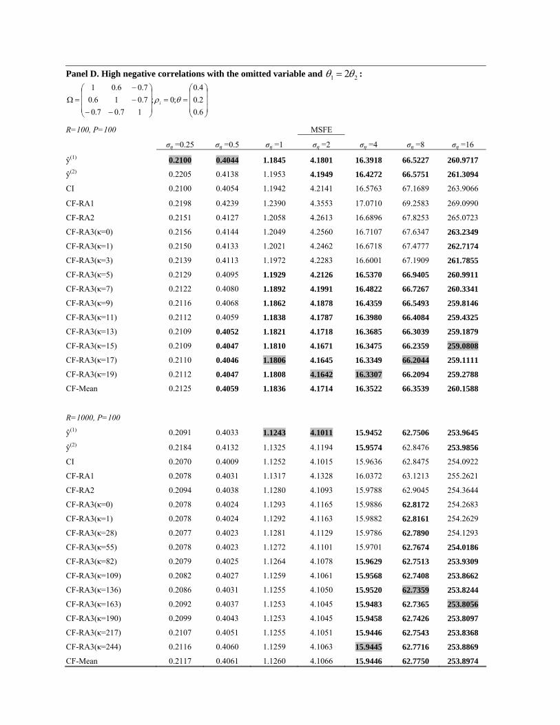
Panel D. High negative correlations with the omitted variable and 21 2θθ = :

⎟⎟⎟

⎠

⎞

⎜⎜⎜

⎝

⎛==

⎟⎟⎟

⎠

⎞

⎜⎜⎜

⎝

⎛

−−−−

=Ω6.02.04.0

;0;17.07.0

7.016.07.06.01

θρi


ŷ(1) 0.2100 0.4044 1.1845 4.1801 16.3918 66.5227 260.9717

ŷ(2) 0.2205 0.4138 1.1953 4.1949 16.4272 66.5751 261.3094

CI 0.2100 0.4054 1.1942 4.2141 16.5763 67.1689 263.9066

CF-RA1 0.2198 0.4239 1.2390 4.3553 17.0710 69.2583 269.0990

CF-RA2 0.2151 0.4127 1.2058 4.2613 16.6896 67.8253 265.0723

CF-RA3(κ=0) 0.2156 0.4144 1.2049 4.2560 16.7107 67.6347 263.2349

CF-RA3(κ=1) 0.2150 0.4133 1.2021 4.2462 16.6718 67.4777 262.7174

CF-RA3(κ=3) 0.2139 0.4113 1.1972 4.2283 16.6001 67.1909 261.7855

CF-RA3(κ=5) 0.2129 0.4095 1.1929 4.2126 16.5370 66.9405 260.9911

CF-RA3(κ=7) 0.2122 0.4080 1.1892 4.1991 16.4822 66.7267 260.3341

CF-RA3(κ=9) 0.2116 0.4068 1.1862 4.1878 16.4359 66.5493 259.8146

CF-RA3(κ=11) 0.2112 0.4059 1.1838 4.1787 16.3980 66.4084 259.4325

CF-RA3(κ=13) 0.2109 0.4052 1.1821 4.1718 16.3685 66.3039 259.1879

CF-RA3(κ=15) 0.2109 0.4047 1.1810 4.1671 16.3475 66.2359 259.0808

CF-RA3(κ=17) 0.2110 0.4046 1.1806 4.1645 16.3349 66.2044 259.1111

CF-RA3(κ=19) 0.2112 0.4047 1.1808 4.1642 16.3307 66.2094 259.2788

CF-Mean 0.2125 0.4059 1.1836 4.1714 16.3522 66.3539 260.1588

R=1000, P=100

ŷ(1) 0.2091 0.4033 1.1243 4.1011 15.9452 62.7506 253.9645

ŷ(2) 0.2184 0.4132 1.1325 4.1194 15.9574 62.8476 253.9856

CI 0.2070 0.4009 1.1252 4.1015 15.9636 62.8475 254.0922

CF-RA1 0.2078 0.4031 1.1317 4.1328 16.0372 63.1213 255.2621

CF-RA2 0.2094 0.4038 1.1280 4.1093 15.9788 62.9045 254.3644

CF-RA3(κ=0) 0.2078 0.4024 1.1293 4.1165 15.9886 62.8172 254.2683

CF-RA3(κ=1) 0.2078 0.4024 1.1292 4.1163 15.9882 62.8161 254.2629

CF-RA3(κ=28) 0.2077 0.4023 1.1281 4.1129 15.9786 62.7890 254.1293

CF-RA3(κ=55) 0.2078 0.4023 1.1272 4.1101 15.9701 62.7674 254.0186

CF-RA3(κ=82) 0.2079 0.4025 1.1264 4.1078 15.9629 62.7513 253.9309

CF-RA3(κ=109) 0.2082 0.4027 1.1259 4.1061 15.9568 62.7408 253.8662

CF-RA3(κ=136) 0.2086 0.4031 1.1255 4.1050 15.9520 62.7359 253.8244

CF-RA3(κ=163) 0.2092 0.4037 1.1253 4.1045 15.9483 62.7365 253.8056

CF-RA3(κ=190) 0.2099 0.4043 1.1253 4.1045 15.9458 62.7426 253.8097

CF-RA3(κ=217) 0.2107 0.4051 1.1255 4.1051 15.9446 62.7543 253.8368

CF-RA3(κ=244) 0.2116 0.4060 1.1259 4.1063 15.9445 62.7716 253.8869

CF-Mean 0.2117 0.4061 1.1260 4.1066 15.9446 62.7750 253.8974

Table 3. Equity Premium Prediction Note: Data range from 1927m1 to 2003m12; “kmax”, the maximum hypothesized number of factors, is set at 12; “h” is the forecast horizon; MSFE is the raw MSFE amplified by 100; MSFE Ratio is the MSFE of each method over that of the Historical Mean model; “k” is the number of factors included in the principal component approaches; “Mean/SD” is the mean and standard deviation of the estimated number of factors over the out-of-sample. The case when Historical Mean benchmark is outperformed is indicated in bold, and the smallest number among them is highlighted.

Panel A1. Monthly prediction, forecasts begin 1969m1 (R=504 and P=420) h=1 h=3 h=6 h=12 MSFE MSFE Ratio MSFE MSFE Ratio MSFE MSFE Ratio MSFE MSFE Ratio Historical Mean 0.0407 0.0407 0.0407 0.0407

CF-Mean 0.0400 0.9820 0.0401 0.9860 0.0403 0.9890 0.0403 0.9891

CF-Median 0.0402 0.9887 0.0404 0.9915 0.0404 0.9913 0.0404 0.9904

CF-RA1 0.0431 1.0585 0.0434 1.0660 0.0420 1.0325 0.0471 1.1548

CF-RA2 0.0447 1.0975 0.0441 1.0847 0.0429 1.0538 0.0457 1.1225

CF-RA3 (κ=0) 0.0439 1.0795 0.0430 1.0581 0.0419 1.0310 0.0457 1.1240

CF-RA3 (κ=1) 0.0434 1.0670 0.0427 1.0487 0.0417 1.0250 0.0452 1.1116

CF-RA3 (κ=3) 0.0425 1.0443 0.0420 1.0317 0.0413 1.0141 0.0443 1.0889

CF-RA3 (κ=5) 0.0417 1.0248 0.0414 1.0172 0.0409 1.0049 0.0435 1.0684

CF-RA3 (κ=7) 0.0410 1.0086 0.0409 1.0052 0.0406 0.9974 0.0427 1.0503

CF-RA3 (κ=9) 0.0405 0.9956 0.0405 0.9956 0.0403 0.9916 0.0421 1.0346

CF-RA3 (κ=11) 0.0401 0.9859 0.0402 0.9884 0.0402 0.9875 0.0416 1.0213

CF-RA3 (κ=13) 0.0398 0.9794 0.0400 0.9837 0.0401 0.9851 0.0411 1.0103

CF-RA3 (κ=15) 0.0397 0.9762 Mean/SD 0.0399 0.9815 Mean/SD 0.0401 0.9844 Mean/SD 0.0408 1.0017 Mean/SD

CF-PC (AIC) 0.0424 1.0429 9.13/3.26 0.0435 1.0697 8.62/3.45 0.0422 1.0363 4.74/4.23 0.0414 1.0158 1.90/2.45

CF-PC (BIC) 0.0400 0.9828 1.30/1.06 0.0405 0.9962 1.14/0.49 0.0408 1.0029 1.18/0.42 0.0407 0.9993 1.06/0.24

CF-PC (k=1) 0.0401 0.9858 0.0403 0.9903 0.0407 0.9989 0.0409 1.0049

CF-PC (k=2) 0.0399 0.9801 0.0405 0.9953 0.0407 1.0000 0.0407 0.9995

CF-PC (k=3) 0.0403 0.9912 0.0410 1.0076 0.0411 1.0090 0.0410 1.0065

CI-Unrestricted 0.0411 1.0103 0.0434 1.0661 0.0424 1.0400 0.0436 1.0712

CI-PC (AIC) 0.0413 1.0142 8.70/2.18 0.0429 1.0537 7.47/2.49 0.0434 1.0655 6.22/2.82 0.0413 1.0147 2.35/0.84

CI-PC (BIC) 0.0428 1.0523 3.29/1.85 0.0434 1.0655 2.48/1.39 0.0427 1.0478 1.92/0.99 0.0410 1.0071 1.38/0.63

CI-PC (k=1) 0.0407 0.9998 0.0407 1.0009 0.0407 0.9996 0.0405 0.9934

CI-PC (k=2) 0.0409 1.0060 0.0413 1.0151 0.0413 1.0134 0.0405 0.9944

CI-PC (k=3) 0.0434 1.0673 0.0440 1.0805 0.0432 1.0612 0.0412 1.0115

Panel A2. Monthly prediction, forecasts begin 1980m1 (R=636 and P=288) h=1 h=3 h=6 h=12

MSFE MSFE Ratio MSFE MSFE Ratio MSFE MSFE Ratio MSFE MSFE Ratio

Historical Mean 0.0398 0.0398 0.0398 0.0398

CF-Mean 0.0395 0.9938 0.0397 0.9980 0.0397 0.9981 0.0398 0.9995

CF-Median 0.0398 0.9993 0.0399 1.0023 0.0397 0.9986 0.0399 1.0026

CF-RA1 0.0422 1.0606 0.0412 1.0361 0.0433 1.0873 0.0424 1.0649

CF-RA2 0.0421 1.0590 0.0423 1.0637 0.0430 1.0811 0.0436 1.0946

CF-RA3 (κ=0) 0.0431 1.0821 0.0422 1.0605 0.0442 1.1108 0.0425 1.0690

CF-RA3 (κ=1) 0.0427 1.0741 0.0420 1.0547 0.0438 1.1008 0.0423 1.0642

CF-RA3 (κ=4) 0.0419 1.0523 0.0413 1.0389 0.0427 1.0734 0.0418 1.0509

CF-RA3 (κ=7) 0.0411 1.0338 0.0408 1.0256 0.0418 1.0501 0.0413 1.0391

CF-RA3 (κ=10) 0.0405 1.0187 0.0404 1.0147 0.0410 1.0310 0.0409 1.0288

CF-RA3 (κ=13) 0.0401 1.0069 0.0400 1.0063 0.0404 1.0161 0.0406 1.0200

CF-RA3 (κ=16) 0.0397 0.9985 0.0398 1.0005 0.0400 1.0053 0.0403 1.0128

CF-RA3 (κ=19) 0.0395 0.9935 0.0397 0.9970 0.0397 0.9986 0.0401 1.0071


CF-PC (AIC) 0.0427 1.0741 10.33/3.27 0.0408 1.0251 8.74/3.98 0.0430 1.0815 9.33/3.95 0.0406 1.0198 4.26/4.55

CF-PC (BIC) 0.0395 0.9937 1.30/0.77 0.0400 1.0063 1.02/0.14 0.0402 1.0104 1.02/0.13 0.0405 1.0161 1/0

CF-PC (k=1) 0.0394 0.9896 0.0399 1.0038 0.0402 1.0089 0.0405 1.0161

CF-PC (k=2) 0.0395 0.9918 0.0402 1.0091 0.0404 1.0154 0.0404 1.0148

CF-PC (k=3) 0.0396 0.9960 0.0401 1.0086 0.0404 1.0150 0.0406 1.0200

CI-Unrestricted 0.0421 1.0592 0.0451 1.1344 0.0419 1.0525 0.0418 1.0495

CI-PC (AIC) 0.0419 1.0522 8.63/1.87 0.0449 1.1274 7.68/2.12 0.0422 1.0607 6.95/2.53 0.0406 1.0197 2.68/1.14

CI-PC (BIC) 0.0423 1.0639 3.02/1.72 0.0421 1.0578 2.35/1.31 0.0406 1.0199 1.64/1.08 0.0413 1.0376 1.56/0.72

CI-PC (k=1) 0.0403 1.0131 0.0404 1.0150 0.0406 1.0200 0.0406 1.0194

CI-PC (k=2) 0.0405 1.0175 0.0408 1.0251 0.0409 1.0274 0.0411 1.0315

CI-PC (k=3) 0.0422 1.0617 0.0423 1.0623 0.0421 1.0575 0.0413 1.0376

Panel B. Quarterly prediction Forecasts begin 1969q1 (R=168 and P=140) Forecasts begin 1980q1 (R=212 and P=96)

h=1 h=4 h=1 h=4

MSFE MSFE Ratio MSFE MSFE Ratio MSFE MSFE Ratio MSFE MSFE Ratio

Historical Mean 0.1518 0.1521 0.1346 0.1347

CF-Mean 0.1455 0.9589 0.1486 0.9768 0.1332 0.9899 0.1356 1.0071

CF-Median 0.1471 0.9689 0.1495 0.9831 0.1345 0.9992 0.1370 1.0172

CF-RA1 0.1888 1.2436 0.2655 1.7457 0.1766 1.3127 0.1692 1.2568

CF-RA2 0.2116 1.3942 0.2510 1.6537 0.1766 1.3120 0.1814 1.3482

CF-RA3 (κ=0) 0.1970 1.2981 0.2539 1.6728 0.2005 1.4901 0.1725 1.2819

CF-RA3 (κ=0.25) 0.1922 1.2660 0.2457 1.6185 0.1958 1.4554 0.1703 1.2656

CF-RA3 (κ=0.5) 0.1875 1.2354 0.2378 1.5665 0.1913 1.4219 0.1682 1.2499


CF-PC (AIC) 0.1994 1.3136 7.08/4.40 0.2051 1.3484 3.31/3.98 0.1645 1.2224 8.69/4.05 0.1476 1.0959 4.17/4.87

CF-PC (BIC) 0.1596 1.0512 1.27/0.66 0.1590 1.0451 1.06/0.23 0.1364 1.0136 1.25/0.78 0.1414 1.0499 1.01/0.10

CF-PC (k=1) 0.1523 1.0036 0.1565 1.0286 0.1344 0.9987 0.1414 1.0501

CF-PC (k=2) 0.1517 0.9993 0.1565 1.0287 0.1369 1.0176 0.1388 1.0306

CF-PC (k=3) 0.1550 1.0214 0.1592 1.0464 0.1375 1.0216 0.1409 1.0467

CI-Unrestricted 0.1645 1.0835 0.1853 1.2182 0.1756 1.3046 0.1619 1.2026

CI-PC (AIC) 0.1744 1.1488 7.66/2.21 0.1689 1.1104 2.56/1.35 0.1741 1.2942 8.73/2.10 0.1442 1.0708 2.97/1.84

CI-PC (BIC) 0.1836 1.2094 2.36/0.95 0.1583 1.0409 1.35/0.78 0.1588 1.1799 2.67/1.60 0.1663 1.2350 2.01/1.49

CI-PC (k=1) 0.1516 0.9991 0.1511 0.9932 0.1401 1.0414 0.1420 1.0543

CI-PC (k=2) 0.1549 1.0207 0.1535 1.0091 0.1459 1.0846 0.1516 1.1257

CI-PC (k=3) 0.1854 1.2214 0.1654 1.0875 0.1630 1.2112 0.1544 1.1467

Panel C. Annual prediction Forecasts begin 1969 (R=42 and P=35) Forecasts begin 1980(R=53 and P=24)

h=1 h=1

MSFE MSFE Ratio MSFE MSFE Ratio

Historical Mean 0.6948 0.4834

CF-Mean 0.6320 0.9096 0.4751 0.9828

CF-Median 0.6524 0.9390 0.4925 1.0188

CF-RA1 3.6004 5.1820 3.1254 6.4651

CF-RA2 2.8360 4.0819 1.5782 3.2646

CF-RA3 (κ=0) 2.9970 4.3141 2.4478 5.0635

CF-RA3 (κ=0.25) 1.5720 2.2625 1.6297 3.3712

CF-RA3 (κ=0.5) 0.7930 1.1408 1.0294 2.1293

CF-RA3 (κ=1) 0.6320 0.9096 Mean/SD 0.4817 0.9965 Mean/SD

CF-PC (AIC) 3.2141 4.6260 10.14/2.59 2.8428 5.8805 10.08/3.39

CF-PC (BIC) 2.5105 3.6133 5.29/4.62 1.0841 2.2426 4.46/4.70

CF-PC (k=1) 0.6971 1.0034 0.5323 1.1012

CF-PC (k=2) 0.6514 0.9376 0.5420 1.1211

CF-PC (k=3) 0.7300 1.0507 0.6323 1.3079

CI-Unrestricted 1.3210 1.9013 0.9659 1.9979

CI-PC (AIC) 1.3247 1.9067 5.34/3.33 0.92799 1.9196 6.33/3.16

CI-PC (BIC) 1.0590 1.5243 3.03/1.87 0.7438 1.5385 1.88/1.33

CI-PC (k=1) 0.7184 1.0340 0.6044 1.2502

CI-PC (k=2) 0.7362 1.0596 0.6373 1.3183 CI-PC (k=3) 0.9556 1.3754 0.6678 1.3814

To Combine Forecasts or to Combine Information

Documents

Transcript of To Combine Forecasts or to Combine Information