DEVELOPING AND PRICING PRECIPITATION INSURANCE

Journal ofAgricultural and Resource Economics 26(1):261-274Copyright 2001 Western Agricultural Economics Association

Developing and PricingPrecipitation Insurance

Steven W. Martin, Barry J. Barnett,and Keith H. Coble

Production agriculture and agribusiness are exposed to many weather-related risks.Recent years have seen the emergence of an increased interest in weather-basedderivatives as mechanisms for sharing risks due to weather phenomena. In thisstudy, a unique precipitation derivative is proposed that allows the purchaser tospecify the parameters of the indemnity function. Pricing methods are presented inthe context of a cotton harvest example from Mississippi. Our findings show apotential for weather derivatives to serve niche markets within U.S. agriculture.

Key words: cross-hedging, precipitation insurance, risk, weather derivative

Introduction

Production agriculture and agribusiness are exposed to many weather-related risks.Common examples include extremes of both precipitation and temperature. In the UnitedStates, the federally subsidized crop insurance program provides crop producers withprotection against many weather-related risks. However, the program is plagued withmoral hazard and adverse selection problems (Skees and Reed; Quiggin, Karagiannis,and Stanton; Smith and Goodwin; Coble et al.; Just, Calvin, and Quiggin). Further,federal crop insurance policies all contain deductibles that leave growers with someexposure to losses associated with extreme weather.

Livestock producers in the U.S. currently have no federally subsidized insurance, yetthey are also exposed to weather risks. Extreme heat can cause increased death loss inbroiler houses and/or higher electrical cost for cooling. Extreme cold can cause increaseddeath loss for range-fed livestock. In 1999, Hurricane Floyd dramatically demonstratedthat extreme precipitation can cause extensive problems with lagoon waste managementsystems for confinement livestock facilities (Barrett; Kilborn; Whitman). Many agri-businesses (input supply, transportation, storage, processing, marketing, etc.) are alsoindirectly affected by impacts of weather risk on production agriculture but have nofederally subsidized insurance.

Recent years have witnessed an increased interest in weather-based derivatives asmechanisms for sharing risks due to weather phenomena. Since early 1997, marketparticipants in the electricity and natural gas sectors have used temperature-based

Steven W. Martin is assistant extension economist at the Delta Research and Extension Center, Mississippi State University;Barry J. Barnett is associate professor, Department of Agricultural and Applied Economics, University of Georgia; and KeithH. Coble is assistant professor, Department of Agricultural Economics, Mississippi State University. This article is based onresearch conducted while Barnett was associate professor in the Department of Agricultural Economics, Mississippi StateUniversity. The authors express their appreciation for the helpful comments of J. Roy Black, Jerry R. Skees, and threeanonymous referees. This research was funded by the Mississippi Agriculture and Forestry Experiment Station.

Review coordinated by J. Scott Shonkwiler and Gary D. Thompson; publication decision made by Gary D. Thompson.

Journal ofAgricultural and Resource Economics

derivatives to offset their exposure to extreme temperatures. Tailored over-the-counterderivatives are based on a specified temperature index such as cumulative heatingdegree days (HDD) or cooling degree days (CDD) for a given location over a specifiedperiod of time (Dischel 1998b). On September 22,1999, the Chicago Mercantile Exchangebegan trading standardized monthly cumulative HDD and CDD futures and optionscontracts. Contracts are now traded for Atlanta, Chicago, Cincinnati, Dallas, Des Moines,Las Vegas, New York, Philadelphia, Portland, and Tucson.

In this article, we propose a unique precipitation derivative that allows the purchaserto specify the parameters of the indemnity function according to his/her risk manage-ment needs. While the proposed derivative has characteristics much like an option, weassume the highly tailored contracts and the relatively small dollar amounts of protectionrequired by most retail purchasers would necessitate sales through traditional retailinsurance channels. A cotton harvest example from Mississippi is employed to demon-strate the potential uses of such derivatives. We begin with a discussion of the rapidlygrowing market for weather derivatives.

Background on Weather Derivatives

Weather derivatives provide a mechanism for cross-hedging against variability in afirm's revenues or costs. If the firm's revenues or costs are sufficiently correlated withthe underlying weather phenomenon, the weather derivative will provide a useful, thoughnot perfect, mechanism for cross-hedging. For example, temperature extremes createproblems for electric and natural gas utilities. During periods of extremely high temper-atures, electric utilities may face levels of consumer demand in excess of generatingcapacity. To meet that demand, utilities purchase marginal quantities of electricity onspot markets. But, because extreme temperatures are often spatially correlated, a utilitymay find itself bidding against many other utilities for available spot market suppliesof electricity. Spot-market prices can increase dramatically above long-run equilibriumlevels. In June 1998, spot-market wholesale prices for electricity increased from $35 permegawatt-hour to $7,500 per megawatt-hour in a matter of days (Dischel 1998c). Whensummer temperatures are unusually mild, electric utilities are faced with reduceddemand and lower revenues. Natural gas suppliers are also faced with temperature-related risks. Unusually mild winter temperatures reduce the demand for natural gas,and hence revenues of natural gas suppliers. Temperature derivatives allow utilities toshed the volumetric risk associated with extreme demand shifts.

Purchasers of weather derivatives are generally exposed to some degree of geograph-ical basis risk. Weather derivatives are typically settled based on realized weatherphenomena, measured by an objective party, at a given location. In the United States,the underlying index is normally based on National Oceanic and Atmospheric Admin-istration (NOAA) measurements at a given weather station. In a world of completeweather derivative contracts, potential purchasers may be able to significantly reducegeographic basis risk by spreading their risk protection across derivatives based onseveral surrounding weather stations.

Weather derivatives are typically based on official NOAA measurements for at leasttwo reasons. First, both parties can be confident of an objective measurement of theweather phenomenon on which the contract will be settled. Second, buyers (sellers) canbase bid (offer) prices on an extended time series of data collected at the site. It is not

262 July 2001

Developing and Pricing Precipitation Insurance 263

unusual for weather data to be available from a given weather station covering periodsof 50 years or more. These data are made available via the internet by the NationalClimate Data Center, a NOAA subsidiary (Dischel 1998c).

Precipitation Insurance

Changnon and Changnon describe the process by which they established premium ratetables for short-term (1-72 hours) precipitation insurance. The policies were designedto provide protection against precipitation affecting outdoor events such as fairs orconcerts. Data from 211 weather stations were used to calculate empirical hourlycumulative frequencies, averaged over calendar months, for six levels of precipitation(0.01, 0.05, 0.10, 0.25, 0.50, and 1.00 inches). The continental United States was dividedinto 17 rating regions, and the historical frequencies were then averaged across all theweather stations within each rating region.

Patrick presents estimated premium costs for a proposed rainfall insurance contractin the Mallee wheat-producing region of Australia. Though Patrick indicates premiumsare derived from "reasonable [parametric] distributions of rainfall," no specifics are pro-vided about distributional forms or parameters.

Sakurai and Reardon estimate the demand for a hypothetical "rainfall lottery" inBurkina Faso. The lottery, which is assumed to be administered by an insurancecompany, would make a lump-sum payment to lottery ticket-holders whenever annualrainfall, measured at a given weather station, is below some predetermined level.

The instruments described by Changnon and Changnon; Patrick; and Sakurai andReardon are similar in that each uses weather station data to calculate premium rates.However, Changnon and Changnon set premium rates for a traditional precipitationinsurance policy where loss adjustment would be based on realized precipitation at theevent site. In contrast, Patrick, and Sakurai and Reardon, consider insurance policieswhich are effectively weather derivatives. Specifically, their studies describe put optionswith loss adjustment based on realized values of an underlying index of precipitationmeasured at a given weather station. Nevertheless, both Patrick, and Sakurai andReardon characterize their proposed precipitation derivatives as insurance, becausethey assume the derivatives would be sold to farmers through retail insurance channels.

Turvey presents stylized European HDD, CDD, and precipitation options where theindemnity function is of the form

O... .0 if x > strike,(1) indemnity = x strike,]

strike-x if x<strikef x <

for puts, and

(2) -indemnity = if x < strike,]x - strike if x > strike

for calls, where strike is a choice variable, x is the cumulative realized value of theunderlying index (HDD, CDD, or precipitation) during the contract period, and X issome predetermined dollar value per unit of the index. Thus, for a precipitation put,if x is 2 inches, strike is 5 inches, and X is $100 per inch, the indemnity would be equalto $300.

Martin, Barnett, and Coble


Skees and Zeuli propose a European precipitation put with an indemnity function ofthe form

0 if x > strike,(3) indemnity = strike - x if strike x liability,

if x < strikestrike

where liability is a choice variable that establishes the maximum possible indemnity.The brackets in equation (3) contain the loss cost function specifying the percentage ofliability to be paid out as an indemnity conditional on the choice of strike and the reali-zation ofx. The indemnity function in equation (3) is analogous to that used by Skees,Black, and Barnett for Group Risk Plan area yield puts. Note, if X = liability/strike,equation (3) is identical to equation (1).

For precipitation, x has a natural lower bound of zero. Thus, for puts, the maximumindemnity is X(strike) for equation (1), and liability for equation (3). But there is nonatural upper bound on x. Thus, for calls, there is no cap on the maximum indemnity.

We propose a more flexible form for European precipitation options. For brevity, wefocus only on calls, though analogous presentations of puts are easily constructed. Theindemnity function for calls is designated by

0 if x < strike,x - strike

(4) indemnity = - strike if limit > x > strike, x liability,limit - strike

1 if x > limit

where limit is an additional choice variable. Again, the brackets contain the loss costfunction for the option. By their choices of strike and limit, purchasers define the domainof x over which the option will pay an indemnity. For calls, limit > strike > 0. In additionto allowing purchasers to tailor the characteristics of precipitation options according totheir risk management needs, the limit variable makes rating of precipitation calls moretractable.

For calls, when limit > strike, we can define a variable ip such that

(5) limit = strike 1 + ),

where 0 < p < oo. Equation (4) can now be rewritten as

0 if x < strike,

p(x - strike)(6) indemnity = ( stri if limit > x > strike, x liability,strike

1 if x > limit

where p is an increasing payment factor. If = 1, limit = 2 x strike. If limit > strike > 0,pj determines how fast the maximum indemnity is paid relative to the base case of limit= 2(strike). Consider a call with the strike set at 6 inches over the contract period. Ifp. = 1, limit will be equal to 12, so the maximum indemnity will be paid only when x is6 inches above the strike. If p = 2, limit will be equal to 9, so the maximum indemnity

264 July 2001


will be paid when x is only 3 inches above the strike. If p = 3, limit will be equal to 8, sothe maximum indemnity will be paid when x is only 2 inches above the strike. Thus, forcalls with the same strike, the value for pj indicates how fast the option will pay the maxi-mum indemnity relative to the base case of p = 1. If p = 2, the call will pay the maximumindemnity twice as fast as the base case; ifp = 3, three times as fast, and so on.

Pricing Precipitation Insurance

Expected loss cost is the standard basis for establishing insurance premium rates (Skeesand Barnett).l Loss cost is equal to indemnities divided by liability. Insurance actuariescalculate an expectation on future loss cost based on historical experience with the insur-ance product. Expected loss cost can be considered as an expected breakeven premiumrate.

Using extended time series of weather data, historical loss costs can be simulated forstylized weather insurance instruments. An expected loss cost can then be estimatedfrom the simulated historical loss costs.

We assume that requiring purchase sufficiently in advance of the contract period willprevent intertemporal adverse selection conditioned on precipitation forecasts (Luo,Skees, and Marchant). In general, advance purchase requirements will need to be setlong enough such that an expectation on precipitation for the contract period conditionedon meteorological forecasts is likely no better than an unconditional expectation. Forsome areas, El Nifo/Southern Oscillation (ENSO) phenomena may require very longadvance purchase requirements (Ker and McGowan; Mjelde, Hill, and Griffiths; Podburyet al.). Alternatively, extensions of the procedures described here could be used to condi-tion premium rates on ENSO phenomena.

Loss cost is the portion of the indemnity function enclosed in brackets in equations(4) and (6). The breakeven premium rate for the proposed precipitation insurance/optionis simply the unconditional expectation of loss cost.

Simulation

Climatological research has supported the use of a gamma distribution to characterizethe distribution of climatological variables (such as cumulative precipitation) exhibitinga physical lower bound of zero but no upper bound (Barger and Thom; Thom; Ison,Feyerherm, and Bark; McWhorter, Matthes, and Brooks; Wax and Walker). The proba-bility density function for the gamma distribution is denoted by

/ )a-l e x pl -a)(7) f(x; c, Pj) x (0;a, p>0,

where x is the random variable (in this case, cumulative precipitation), a is the shapeparameter, and p is the scale parameter. The mean of the distribution is ap.

1While the proposed precipitation insurance is, in essence, an option, pricing based on standard options valuation modelsis problematic. Standard options valuation models require that one be able to construct (at least conceptually) a riskless port-folio consisting of both the option and the asset which forms the underlying index (Hull; Dischel 1998a). Yet, there is noactively traded forward market for precipitation.



To initiate the simulation, cumulative precipitation measures over the chosen contractperiod are calculated for each year in the historical data series. Maximum-likelihoodestimation is then applied to these data to estimate the parameters on the gammadistribution. Because the natural log of zero is undefined, a statistical problem occursif any of the cumulative precipitation observations in the historical data series are equalto zero. To address this problem, Wilks treats precipitation data as exhibiting type Icensoring on the left. In the United States, precipitation amounts of less than 0.01 inchare not recorded in official measurements. If we designate the censoring point as C,

where 0 < C < 0.01, then a given set of cumulative precipitation data will contain Nccensored years in which cumulative precipitation over the contract period is recordedas zero, and Nw years with positive measured values. The total number of years in thedata set will be equal to Nc + Nw. Wilks specifies the likelihood function for the param-eters of the assumed gamma distribution as follows:

Nc Nw

(8) L(a, P; x) = HF(C; a, P) nf(xi; a, P)j=1 i=1

(x 1 ( -xN W - exp-

=[F(C; a, P)]NC P pi=1 p(a

where F is the cumulative distribution function,

(9) F(C; a, P) = Cf(x; a, P)dx = Pr{xj < C}.

The log-likelihood function to be maximized is written as

(10) A(a, P; x) = Ncln[F(C; a, P)] - Nw[aln(P) + ln[r(a)]]Nw 1 Nw

(a-1)ln(xi) - -i=l P i=1

Note that if Nc = 0, equation (10) reduces to the standard log-likelihood function forfitting the parameters of a gamma distribution.

Figure 1 presents estimated gamma probability density functions over cumulativedaily precipitation for the weather station located at the Delta Research and ExtensionCenter (DREC) in Stoneville, Mississippi. The probability density functions are basedon data from 1936 through 1995. The associated parameter estimates and standarderrors are found in table 1. All distributions exhibit positive skewness. Yet, as thetime period lengthens, the distributions become more symmetric. This is consistentwith findings reported in climatological literature suggesting more symmetric distri-butions may adequately characterize cumulative precipitation measured seasonallyor annually, but are unlikely to be appropriate for shorter time periods. Climatologistsprefer the gamma distribution because it is sufficiently flexible to adequately character-ize cumulative precipitation over time periods of varying length (McWhorter, Matthes,and Brooks).

After fitting the parameters of the gamma distribution, the expectation of loss costis calculated by integrating over the loss cost component of the indemnity function. Fora call, the expectation of loss cost corresponding to equation (4) is given by

266 July 2001


U .'U

0.35

0.30

0.25

.2co 0.20.00

a. 0.15

0.10

0.05

0.00

0 1 2 3 4 5 6 7 8 9 10 11 12 13 14 15 16 17 18 19 20

Inches of Precipitation

Figure 1. Estimated gamma probability density functions forprecipitation at the Delta Research and Extension Center,based on daily precipitation data, 1936-1995

(11) E(loss cost) = limit x- strike f(x)dx + f(x)dxJstrike limit -strike) limit

where f(x) is the gamma density. This expression can be rewritten to correspond toequation (6) as follows:

(12) E(loss cost) = imit((x - strike) f(x)dx+ f(x)dx.istrike strike imit

No indemnity is paid if x < strike.

Results

A cotton harvest example is used to illustrate the procedure described above. In the mid-South, cotton harvest generally occurs during the period from mid-September until theend of October. Growers in the region typically defoliate the crop when approximately70% of the bolls are open. However, precipitation between the time cotton bolls open andharvest can cause significant reductions in revenue. These losses occur due to lost yieldand reduced quality.

Using data from DREC test plots, Williford et al. estimate per acre revenue lossesbetween defoliation and harvest due to various discrete levels of precipitation. Theyassume a 650 pound per acre expected yield and an expected price of $0.60 per pound.We fit a quadratic function to these data to obtain the continuous loss function:

(13) loss per acre = -5.02 + 15.0757z - 0.3166z 2

(2.07) (0.60) (0.04)

R2 = 0.997,


A An .

I


Table 1. Gamma Distribution Parameter Estimates Based on Daily Precipi-tation Measurements

ShapeParameter, a Mean, aU

Weather Station (Standard Error) (Standard Error)

Delta Research & Extension Center, Stoneville, Mississippi 4.24 6.41September 1-October 31 (1936-1995) (0.766) (0.413)

Delta Research & Extension Center, Stoneville, Mississippi 1.88 3.25October 1-October 31 (1936-1995) (0.327) (0.314)

Delta Research & Extension Center, Stoneville, Mississippi 1.19 1.94October 16-October 31 (1936-1995) (0.201) (0.250)

Greenville, Mississippi 1.21 2.89October 1-October 31 (1936-1995) (0.199) (0.339)

Cleveland, Mississippi 1.25 3.19October 1-October 31 (1936-1988) (0.219) (0.392)

where z is precipitation between defoliation and harvest, and the numbers in parenthesesare standard errors. The loss function is shown in figure 2. On a hypothetical 1,000-acrecotton farm, 4 inches of cumulative precipitation cause an estimated loss of approxi-mately $50,200; 6 and 8 inches of cumulative precipitation cause estimated losses ofapproximately $74,000 and $95,300, respectively.

Suppose, prior to planting, this grower purchased a buy-up insurance policy covering65% of the actual production history (APH) yield at 100% of the expected price (the mostcommon selections on buy-up policies). For simplicity, assume theAPH yield is equalto the expected yield of 650 pounds per acre. Also assume a price selection equal to theexpected price of $0.60 per pound. The expected revenue on the crop is $390,000. Yet,because of the 35% deductible, the grower is responsible for the first $136,500 of yieldor quality losses (realized yield is adjusted for quality losses on crop yield insurancepolicies). Suppose further that in late September the crop is on target to meet the 650pound per acre yield expectation. The grower is concerned about potential losses due toprecipitation prior to harvest. At this time, the crop yield insurance policy providesessentially no financial protection because of the deductible. Historical data from 1936-1995 reveal mean cumulative precipitation for October at the DREC of 2.96 inches, witha range from 0.03 to 10.99 inches. Twelve inches of precipitation, higher than any occur-rence in the historical record, would generate an estimated $130,300 in losses, all ofwhich would fall under the grower's deductible. Even with a 75% coverage level, a cropyield insurance policy would not pay an indemnity until over 8 inches of precipitationhad caused almost $100,000 in losses. If, in late September, the expected yield on thecrop is higher (lower) than the APH yield, higher (lower) losses due to precipitation wouldbe required to trigger a crop yield insurance indemnity.

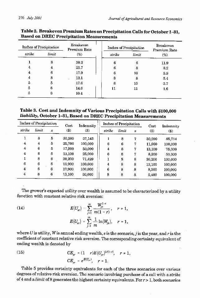
We construct a precipitation call for the period October 1-October 31, with the under-lying index being precipitation measured at the DREC. Table 2 presents breakevenpremium rates for various strikes and limits.

For different choices of strike and limit, and different realizations ofx, table 3 reports thecost and indemnity for a call with liability equal to $100,000. Various combinations ofstrike and limit would provide protection against the estimated losses. Breakeven premiumcosts range from $30,200 for strike = 1 and limit = 8, to $5,400 for strike = limit = 8.

268 July 2001


140

120

100

a)o 80

a(

cn0U0-J 40

20

O1 2 3 4 5 6 7 8 9 10 11 12

Inches of Precipitation

Source: Adapted from Williford et al.

Figure 2. Estimated losses per acre on cotton due to precipitationbetween defoliation and harvest

While various combinations are possible, consider a few examples. If realized precipi-tation is 6 inches, total losses would be approximately $74,000. A $100,000 call with astrike of 4 inches and a limit of 6 inches would have a breakeven cost of $17,900. With

the realized precipitation of 6 inches, the call would pay an indemnity of $100,000. This

would more than cover the estimated loss. A $100,000 call with a strike of 4 inches anda limit of 8 inches would have a breakeven cost of $13,100 and, given the same realizedprecipitation, would pay an indemnity of $50,000, covering only about two-thirds of theestimated loss.

A grower may wish to spread his/her liability across multiple options. Continuing ourexample, a grower could purchase a $50,000 call with a strike of 4 inches and a limit of6 inches, and a $50,000 call with a strike of 4 inches and a limit of 8 inches. This combin-ation would have a breakeven cost of $15,500 and would pay an indemnity of $75,000for 6 inches of realized rainfall. By spreading liability across multiple options with

different combinations of strike and limit, options purchasers can attempt to better match

indemnities to anticipated losses over the domain of potential precipitation.We conduct an expected utility analysis to test the efficacy of these instruments in

protecting against precipitation-induced cotton losses prior to harvest. Our hypothetical1,000-acre farm, located at the Delta Research and Extension Center, is assumed to havean initial wealth of $400,000. Using the loss function in equation (13), pre-harvest losses

are estimated for each year from 1936 through 1995 based on cumulative precipitation

from October 1-31. Table 4 presents mean ending wealth and the standard deviation

of ending wealth under three scenarios: (a) no purchase of precipitation derivatives,(b) purchase of a $100,000 call for DREC with a strike of 4 inches and a limit of 8 inches,and (c) purchase of a $100,000 call for DREC with a strike of 1 inch and a limit of 8inches.


I


Table 2. Breakeven Premium Rates on Precipitation Calls for October 1-31,Based on DREC Precipitation Measurements

Breakeven BreakevenInches of Precipitation re Rae Inches of Precipitation BreakePremium Rate Premium Ratestrike limit (%) strike limit (%)

1 8 30.2 6 6 11.94 4 25.7 6 8 8.24 6 17.9 6 10 5.94 8 13.1 8 8 5.45 5 17.6 8 10 3.75 6 14.6 11 11 1.65 8 10.4

Table 3. Cost and Indemnity of Various Precipitation Calls with $100,000liability, October 1-31, Based on DREC Precipitation Measurements

Inches of Precipitation Inches of PrecipitationCost Indemnity Cost Indemnitystrike limit x ($) ($) strike limit x ($) ($)

1 8 5 30,200 57,143 1 8 7 30,200 85,7144 4 5 25,700 100,000 6 6 7 11,900 100,0004 6 5 17,900 50,000 4 8 7 13,100 75,0004 8 5 13,100 25,000 6 8 7 8,200 50,0001 8 6 30,200 71,429 1 8 8 30,200 100,0006 6 6 11,900 100,000 4 8 8 13,100 100,0004 6 6 17,900 100,000 6 8 8 8,200 100,0004 8 6 13,100 50,000 8 8 8 5,400 100,000

The grower's expected utility over wealth is assumed to be characterized by a utilityfunction with constant relative risk aversion:

(14)m W

1n-rm IWlr

E(Usr) = E JS r s1j=1 m(l - r)m 1

E(Usr) = E ln(Wjs), r =1,j=1 m

where U is utility, Wis annual ending wealth, s is the scenario, j is the year, and r is thecoefficient of constant relative risk aversion. The corresponding certainty equivalent ofending wealth is denoted by

(15) CEsr = (1 - r)E(Usr)/(l'r), r 1,

CEs = eE(Ur), r = 1.

Table 5 provides certainty equivalents for each of the three scenarios over variousdegrees of relative risk aversion. The scenario involving purchase of a call with a strikeof 4 and a limit of 8 generates the highest certainty equivalents. For r > 1, both scenarios

270 July 2001


Table 4. Summary Statistics on Ending Wealth Assuming Purchase of October1-31 Precipitation Calls, Based on DREC Precipitation Measurements

Ending Wealth ($)

Call Scenario Mean Std. Deviation

No Purchase 364,633 30,136strike = 4, limit = 8 364,854 16,082strike = 1, limit = 8 363,264 4,580

Table 5. Certainty Equivalents Assuming Purchase of October 1-31 Precipita-tion Calls, Based on DREC Precipitation Measurements

Call ScenarioConstant RelativeRisk Aversion No Purchase strike = 4, limit = 8 strike = 1, limit = 8

-------------- Certainty Equivalents ($)--------------1.0 363,338 364,504 363,2361.5 362,662 364,328 363,2222.0 361,966 364,152 363,2082.5 361,251 363,976 363,1943.0 360,517 363,800 363,1794.0 358,988 363,447 363,151

involving purchase of a precipitation call generate higher certainty equivalents than thescenario with no purchase. The certainty equivalent for a purchase scenario is less thanthat of a no-purchase scenario only when r = 1 and the call has a strike of 1 and a limitof 8.

To assess the impact of geographic basis risk, the same scenarios are tested with thecalls based on weather stations located in Greenville and Cleveland, Mississippi (tables6 and 7). Greenville, Mississippi, is located approximately 11 miles west and slightlysouth of DREC. Cleveland, Mississippi, is situated approximately 31 miles north andslightly east of DREC. Daily precipitation data were available for 1936-95 for Greenvilleand 1936-88 for Cleveland. (Parameter estimates for the underlying gamma distributionsare shown in table 1.)

Table 6 reports mean ending wealth and the standard deviation of ending wealth forcalls based on Greenville and Cleveland, Mississippi, and table 7 presents certaintyequivalents for the calls. For every value of r, the certainty equivalents of the purchasescenarios exceed those of the no-purchase scenario. The calls based on DREC andGreenville generate lower standard deviations of ending wealth than those based onCleveland. However, the calls based on Cleveland cost less than those based on DRECand Greenville. As a result, the highest certainty equivalents generally occur with thepurchase of calls based on Cleveland-the location farthest away from the hypotheticalfarm. The only exception is for the call with strike = 4 and limit = 8 at the higher levelsof r. In this case, calls based on DREC generate higher certainty equivalents than thosebased on Cleveland. Thus, for these examples, basis risk does not significantly underminethe benefits of purchasing precipitation calls.



Table 6. Summary Statistics on Ending Wealth Assuming Purchase of October1-31 Precipitation Calls, Based on Greenville and Cleveland, Mississippi, Pre-cipitation Measurements

Ending Wealth ($)

Weather Station/Call Scenario Mean Std. Deviation

Greenville: strike = 4, limit = 8 364,610 17,788

Greenville: strike = 1, limit = 8 364,629 12,818

Cleveland: strike = 4, limit = 8 365,284 19,470

Cleveland: strike = 1, limit = 8 364,936 14,483

Table 7. Certainty Equivalents Assuming Purchase of October 1-31 Precipi-tation Calls, Based on Greenville and Cleveland, Mississippi, PrecipitationMeasurements

Greenville Call Scenarios Cleveland Call Scenarios

Constant Relative strike = 4, strike = 1, strike = 4, strike = 1,Risk Aversion limit = 8 limit = 8 limit = 8 limit = 8

--------------- Certainty Equivalents ($)---------------1.0 364,181 364,408 364,767 364,6551.5 363,966 364,297 364,505 364,5142.0 363,750 364,187 364,241 364,3732.5 363,534 364,076 363,975 364,2313.0 363,318 363,966 363,706 364,0904.0 362,885 363,746 363,162 363,808

Conclusion

Interest in weather derivatives is growing rapidly. To date, most applications in theUnited States have been in nonagricultural industries. However, several other countriesare attempting to use weather derivatives in agricultural applications. While the currentfederal crop insurance program crowds out some demand, weather derivatives couldpossibly serve niche markets within U.S. agriculture.

We propose a flexible precipitation insurance/option instrument that allows the pur-chaser to specify various parameters of the indemnity function. We also present a proposedrating method based on simulation procedures. The choice variable, limit, allows buyersto define a layer of protection over the domain of potential precipitation. This featurecan alternatively be characterized as an increasing payment factor reflecting the rateat which the maximum indemnity will be paid relative to a base case. The limit variablehas numerous potential applications beyond precipitation options. For example, itsadoption would likely improve the efficiency of other index options such as federal cropinsurance Group Risk Plan contracts.

Further research could address the potential for reducing geographical basis risk byspreading liability across contracts purchased on several surrounding weather stations.

272 July 2001


Alternatively, insurers, or other weather brokers, could use geographical smoothingtechniques to base indemnities and premiums on some algebraic combination ofweather-station measurements. Further research is also required to determine appropriateadvance purchase requirements for different climatological regions. Should meteor-ologists develop procedures that accurately predict ENSO occurrences on a consistentbasis, the rating procedures described here could be modified to allow for conditionalexpectations on loss cost.

[Received November 1999; final revision received February 2001.]

References

Barger, G. L., and H. C. S. Thornm. "Evaluation of Drought Hazard." Agronomy J. 41(November 1949):519-26.

Barrett, B. "Hog Waste Escapes Dozens of Lagoons as Neuse Rises." The News & Observer (19 September1999). Online. Available at http://www.news-observer.com/daily/1999/09/19/ncO7.html.

Changnon, S. A., and J. M. Changnon. "Developing Rainfall Insurance Rates for the Contiguous UnitedStates." J. Appl. Meteorology 28(November 1989):1185-96.

Coble, K. H., T. 0. Knight, R. D. Pope, and J. R. Williams. "An Expected-Indemnity Approach to theMeasurement of Moral Hazard in Crop Insurance."Amer. J. Agr. Econ. 79(February 1997):216-26.

Dischel, R. "Options Pricing: Black-Scholes Won't Do." Energy and Power Risk Management. Weatherrisk special report, October 1998a.

. "The Fledgling Weather Market Takes Off: Weather Sensitivity, Weather Derivatives, and aPricing Model." Appl. Derivatives Trading 32(November 1998b). Online. Available at http://www.adtrading.com/adt32/weather 1.hts.

. "The Fledgling Weather Market Takes Off: Weather Data for Pricing Weather Derivatives."Appl. Derivatives Trading 33(December 1998c). Online. Available at http://www.adtrading.com/adt33/weather2.hts.

Hull, J. C. Options, Futures, and Other Derivatives, 4th ed. Upper Saddle River NJ: Prentice-Hall, 2000.Ison, N. T., A. M. Feyerherm, and L. D. Bark. "Wet Period Precipitation and the Gamma Distribution."

J. Appl. Meteorology 10(1971):658-65.Just, R. E., L. Calvin, and J. Quiggin. "Adverse Selection in Crop Insurance: Actuarial and Asymmetric

Information Incentives." Amer. J. Agr. Econ. 81(November 1999):834-49.Ker, A. P., and P. J. McGowan. "Weather-Based Adverse Selection and the U.S. Crop Insurance Pro-

gram: The Private Insurance Company Perspective." J. Agr. and Resour. Econ. 25(December 2000):386-410.

Kilborn, P. T. "Hurricane Reveals Flaws in Farm Law." New York Times (17 October 1999). Online.Available at http://www.nytimes.com/library/national/101799floyd-environment.html.

Luo, H., J. R. Skees, and M. A. Marchant. "Weather Information and the Potential for IntertemporalAdverse Selection in Crop Insurance." Rev. Agr. Econ. 16(1994):441-51.

McWhorter, J. C., R. K. Matthes, Jr., and B. P. Brooks, Jr. "Precipitation Probabilities for Mississippi."Staff pap., Water Resources Research Institute, Mississippi State University, 1966.

Mjelde, J. W., S. J. Hill, and J. F. Griffiths. "A Review of Current Evidence on Climate Forecasts andTheir Economic Effects in Agriculture." Amer. J. Agr. Econ. 80,5(1998):1089-95.

Patrick, G. F. "Mallee Wheat Farmers' Demand for Crop and Rainfall Insurance."Austral. J. Agr. Econ.32(April 1988):37-49.

Podbury, T., T. C. Sheales, I. Hussain, and B. S. Fisher. "Use of El Nifno Climate Forecasts in Australia."Amer. J. Agr. Econ. 80,5(1998):1096-1101.

Quiggin, J., G. Karagiannis, and J. Stanton. "Crop Insurance and Crop Production: An Empirical Studyof Moral Hazard and Adverse Selection." In Economics of Agricultural Crop Insurance, eds., D. L.Hueth and W. H. Furtan, pp. 253-72. Norwell MA: Kluwer Academic Publishers, 1994.



Sakurai, T., and T. Reardon. "Potential Demand for Drought Insurance in Burkina Faso and Its Deter-minants." Amer. J. Agr. Econ. 79(November 1997):1193-1207.

Skees, J. R., and B. J. Barnett. "Conceptual and Practical Considerations for Sharing Catastrophic/Systemic Risks." Rev. Agr. Econ. 21(Fall/Winter 1999):424-41.

Skees, J. R., R. J. Black, and B. J. Barnett. "Designing and Rating an Area Yield Crop InsuranceContract." Amer. J. Agr. Econ. 79(May 1997):430-38.

Skees, J. R., and M. R. Reed. "Rate-Making and Farm-Level Crop Insurance: Implications for AdverseSelection." Amer. J. Agr. Econ. 68(August 1986):653-59.

Skees, J. R., and K. A. Zeuli. "Using Capital Markets to Increase Water Market Efficiency." Paperpresented at the 1999 International Symposium on Society and Resource Management, Brisbane,Australia, 8 July 1999.

Smith, V. H., and B. K. Goodwin. "Crop Insurance, Moral Hazard, and Agricultural Chemical Use."Amer. J. Agr. Econ. 78(May 1996):428-38.

Thom, H. C. S. "A Note on the Gamma Distribution." Monthly Weather Rev. 86(April 1958):117-21.Turvey, C. G. "Weather Insurance, Crop Production, and Specific Event Risk." Paper presented at

annual meetings of the AAEA, Nashville TN, 8-11 August 1999.Wax, C. L., and J. C. Walker. "Climatological Patterns and Probabilities of Weekly Precipitation in

Mississippi." Info. Bull. No. 79, Mississippi Agr. and Forestry Exp. Sta., January 1986.Whitman, D. "Hell in High Water." U.S. News and World Report (4 October 1999). Online. Available at

http://www.usnews.com/usnews/issue/991004/flood.htm.Wilks, D. S. "Maximum Likelihood Estimation for the Gamma Distribution Using Data Containing

Zeros." J. Climate 3(December 1990):1495-1501.Williford, J. R., F. T. Cooke, Jr., D. F. Caillavet, and S. Anthony. "Effect of Harvest Timing on Cotton

Yield and Quality." Proceedings of the Beltwide Cotton Conferences 26(1995):633-38.

274 July 2001

DEVELOPING AND PRICING PRECIPITATION INSURANCE

Documents

Transcript of DEVELOPING AND PRICING PRECIPITATION INSURANCE