DYNAMIC PRICING OF GENERAL INSURANCE IN A COMPETITIVE MARKET
34
DYNAMIC PRICING OF GENERAL INSURANCE IN A COMPETITIVE MARKET BY P AUL EMMS ABSTRACT A model for general insurance pricing is developed which represents a sto- chastic generalisation of the discrete model proposed by Taylor (1986). This model determines the insurance premium based both on the breakeven premium and the competing premiums offered by the rest of the insurance market. The opti- mal premium is determined using stochastic optimal control theory for two objective functions in order to examine how the optimal premium strategy changes with the insurer’s objective. Each of these problems can be formu- lated in terms of a multi-dimensional Bellman equation. In the first problem the optimal insurance premium is calculated when the insurer maximises its expected terminal wealth. In the second, the premium is found if the insurer maximises the expected total discounted utility of wealth where the utility function is nonlinear in the wealth. The solution to both these problems is built-up from simpler optimisation problems. For the terminal wealth problem with constant loss-ratio the optimal premium strategy can be found analytically. For the total wealth problem the optimal relative premium is found to increase with the insurer’s risk aversion which leads to reduced market exposure and lower overall wealth generation. 1. INTRODUCTION Dynamic programming has found widespread application in both finance and insurance originating with the optimal asset allocation problem (Samuelson 1969, Merton 1971; 1990). Merton found the optimal allocation of resources in a portfolio consisting of a risky asset and a risk-free asset in order to max- imise some measure of wealth. Part of the attraction of the theory is that the optimal strategy can be determined in closed-form under certain assumptions concerning the form of the process describing the risky asset and the objective of the portfolio manager. The strategy is dynamic since it uses information as it arises: the optimal strategy can be determined as long as we specify the distributions of the underlying processes and the current values of the state variables. There are many generalisations of the problem in the literature includ- ing, for example, an N dimensional state space, non-Markov underlying processes, Astin Bulletin 37(1), 1-34. doi: 10.2143/AST.37.1.2020796 © 2007 by Astin Bulletin. All rights reserved.
Transcript of DYNAMIC PRICING OF GENERAL INSURANCE IN A COMPETITIVE MARKET

DYNAMIC PRICING OF GENERAL INSURANCEIN A COMPETITIVE MARKET
BY
PAUL EMMS
ABSTRACT
A model for general insurance pricing is developed which represents a sto-chastic generalisation of the discrete model proposed by Taylor (1986). This modeldetermines the insurance premium based both on the breakeven premium andthe competing premiums offered by the rest of the insurance market. The opti-mal premium is determined using stochastic optimal control theory for twoobjective functions in order to examine how the optimal premium strategychanges with the insurer’s objective. Each of these problems can be formu-lated in terms of a multi-dimensional Bellman equation.
In the first problem the optimal insurance premium is calculated when theinsurer maximises its expected terminal wealth. In the second, the premium isfound if the insurer maximises the expected total discounted utility of wealthwhere the utility function is nonlinear in the wealth. The solution to both theseproblems is built-up from simpler optimisation problems. For the terminalwealth problem with constant loss-ratio the optimal premium strategy can befound analytically. For the total wealth problem the optimal relative premiumis found to increase with the insurer’s risk aversion which leads to reducedmarket exposure and lower overall wealth generation.
1. INTRODUCTION
Dynamic programming has found widespread application in both finance andinsurance originating with the optimal asset allocation problem (Samuelson1969, Merton 1971; 1990). Merton found the optimal allocation of resourcesin a portfolio consisting of a risky asset and a risk-free asset in order to max-imise some measure of wealth. Part of the attraction of the theory is that theoptimal strategy can be determined in closed-form under certain assumptionsconcerning the form of the process describing the risky asset and the objectiveof the portfolio manager. The strategy is dynamic since it uses informationas it arises: the optimal strategy can be determined as long as we specify thedistributions of the underlying processes and the current values of the statevariables. There are many generalisations of the problem in the literature includ-ing, for example, an N dimensional state space, non-Markov underlying processes,
Astin Bulletin 37(1), 1-34. doi: 10.2143/AST.37.1.2020796 © 2007 by Astin Bulletin. All rights reserved.
9784-07_Astin37/1_01 30-05-2007 13:50 Pagina 1

and random time horizons. Reviews of the literature are contained in Karatzas &Shreve (1998) and Campbell & Viceira (2001).
In actuarial science there are a number of established problems which havebeen tackled using dynamic programming. The optimal asset allocation problemfor an insurer was investigated by Browne (1995). The problem is more com-plex for an insurance company because it invests in risky assets in order tomaintain a reserve to pay out incoming claims. There are then at least two, pos-sibly correlated, random processes required for the model: the invested assetand the claims process. Browne used a normal random process to model thecash flow and found it is optimal to invest a fixed amount of the reserve if theobjective is to maximise the expected utility of wealth for an exponential utilityfunction. He also found that this strategy corresponds to minimising the prob-ability of ruin when the risk-free interest rate is zero. Hipp & Plum (2000) con-sidered the problem with a compound Poisson process for the claims process:the optimal strategy now depends on the current value of the insurer’s reserve.Other insurance problems which use dynamic programming include optimalproportional reinsurance (Højgaard & Taksar 1997), optimal new businessgeneration (Hipp & Taksar 2000) and optimal dividend payout for an insurer(Asmussen & Taksar 1997). A comprehensive review of optimal control theoryapplied to insurance can be found in Hipp (2004).
In this paper we determine the optimal premium strategy for an insurer whichmaximises a particular objective over a fixed planning horizon. Actuaries tradi-tionally price insurance through a premium principle, which relates the charge forcover to the moments of the claims distribution. In this work we determine the pre-mium by using a competitive demand model (following Taylor 1986) as well as theexpected claim size. Consequently, we suppose that the premium is determinedin part by the price relative to the rest of the insurance market. It is not enoughthat an insurer set a price to cover claims if the rest of the market undercuts thatprice since then the insurer will gain insufficient income to remain viable.
The demand law specifies how the insurer’s income and exposure changewith the relative to market premium: a low relative premium generates expo-sure but leads to reduced premium income. The approach builds on the workin Emms, Haberman & Savoulli (2007) and Emms & Haberman (2005), butdevelops a more sophisticated and realistic model, so that the dependence ofthe optimal strategy on the current state is stochastic. Emms, Haberman &Savoulli (2007) developed a continuous time version of Taylor’s model (Tay-lor 1986) because continuous time control systems are often easier to analysethan discrete problems. However, the continuous time version of Taylor’s modelleads to a bang-bang optimal premium strategy which is not realistic. Conse-quently, Emms & Haberman (2005) developed an accrued premium pricingmodel by supposing that the continuously varying premium is paid at a ratefixed at the start of the policy. Here, we also suppose that the premium is acontinuous process; however, policyholders are assumed to pay a fixed amountat the start of the policy in return for a constant period of cover. A renewalof insurance is treated as if the policyholder were buying a new period ofcover. This assumption reduces the state space of the optimisation problem and
2 P. EMMS
9784-07_Astin37/1_01 30-05-2007 13:50 Pagina 2

so makes the analysis easier. Emms & Haberman (2005) determined the optimalpremium strategy which maximised the expected terminal wealth of the insurer.We examine a terminal wealth and a total wealth objective and assess the qual-itative impact of this change on the optimal premium strategy.
In Section 2 we propose a two factor model of the general insurance market:one factor models the randomness of the claim size and intensity, whilst theother models the market average premium. This model is used to determine thepremium which maximises a number of possible objective functions of theinsurer. Section 3 describes the derivation of the Bellman equation which givesthe optimal dynamic premium strategy to maximise the expected terminal wealthof the insurer. The problem reduces to the solution of a reaction-diffusionequation, which is straightforward to solve numerically. Next in Section 4 weconsider the objective of maximising the expected total discounted utility ofwealth with a utility function linear in the wealth. This is probably a morerealistic objective for an insurer given the regulatory constraints imposed overthe course of the planning horizon. The resulting reaction-diffusion equationis slightly more complex but it is again straightforward to solve numerically.We consider a nonlinear utility function by constructing a perturbation expansionin the risk aversion of the insurer. This leads to a pair of coupled reaction-dif-fusion equations and a numerical solution gives the optimal premium strategy.Finally in Section 5 we compare the strategies and suggest further work.
2. MARKOV MODEL
Emms, Haberman & Savouilli (2007) extended Taylor’s model to the case thatthe market average premium is stochastic and the breakeven premium is con-stant. Here we generalise further by adopting stochastic processes with givendistributions for the market average premium pt (per unit exposure) and theloss-ratio gt. Since the market average premium is positive we suppose that itis lognormally distributed:
dpt = pt(mdt + s1d W1t), (1)
where the drift m and the coefficient of volatility s1 are constants and W1t is aBrownian motion. Note that all premiums are specified as per unit of exposureso that each policyholder pays the same premium irrespective of the exposurethat is being insured. Hereafter we shall omit this qualification.
We introduce the relative loss ratio which we define as the ratio between thebreakeven premium pt of the insurer and the market average premium1:
t .gppt
t= (2)
DYNAMIC PRICING OF GENERAL INSURANCE IN A COMPETITIVE MARKET 3
1 In the actuarial literature the loss ratio is usually defined as the claims divided by the premiumsreceived by a company over a year (Daykin et al. 1994).
9784-07_Astin37/1_01 30-05-2007 13:50 Pagina 3
The breakeven premium is the random amount a policy of length t costs theinsurance company. This is the actuarial premium without any profit marginand can be deduced from the insurer’s previous claims data and a loading fac-tor to account for expenses and interest rates (Daykin & Hey 1990). Ratherthan complicating the model with a precise formulation for this factor we sup-pose that the breakeven premium is a stochastic process (Pentikäinen 1986).The advantage of this formulation is that there are no outstanding liabilitiesat the end of the planning horizon T because as soon as policies of total expo-sure dqt are bought, the insurer sets aside pt dqt to cover the resulting claims.Appendix A describes the modifications to the theory if we adopt a stochasticprocess for the mean claim size rate.
We expect a direct correlation between the premium that the market chargesand the breakeven premium of the insurer. If we suppose that claims are identi-cally distributed for the market and the individual insurer then the discrepancybetween these quantities represents the different loadings that insurance compa-nies apply to their policies. Consequently we suppose that the log of the loss-ratiois a Vasicek process (gt must be positive) and that the mean of log gt reverts to zero:
d log gt = – r log gt dt + s2 d W2t,
where r is the rate of reversion, s2 is the coefficient of volatility and W2t is aBrownian motion independent of W1t. Ito’s Lemma gives the SDE for gt as
dgt = gt [ 2
1 s22 – r log gt ] dt + s2gt d W2t. (3)
This definition forces the market average premium towards the breakeven pre-mium: � [gt ] = es2
2 /4r as t → ∞. Market data often show the market average pre-mium drifting above and below the breakeven premium so this would seem tobe a reasonable model (Daykin et al. 1994).
Suppose a policyholder pays a premium p(t) to the insurer at the start ofthe policy for a fixed term of insurance cover t. We suppose that at the end ofthe cover the policyholder can renew by paying p(t + t), that is the same pre-mium as that charged to new business. We suppose the insurer writes a numberof these policies in a time interval dt generating total exposure dqt and receivesthe premium income ptdqt in return. Thus pt is the premium charged to newpolicyholders and existing policyholders who want to renew their policies.
The model is completed by evolution equations for the insurer’s exposureqt and wealth wt. We suppose that the rate of generation of new and renewedexposure bt is parameterised as
bt = qtG(kt), (4)
where G is a demand function which represents the fractional increase in expo-sure per unit time arising from the relative premium charged, kt, defined by
kt = pt /pt.
4 P. EMMS
9784-07_Astin37/1_01 30-05-2007 13:50 Pagina 4

Consequently the wealth generated by premium income over time dt due to afractional increase in exposure is pt dqt = ptbt dt.
This notation leads to the following SDEs:
dq t = (bt – kqt)dt, (5)
dwt = – awtdt + (pt – pt)btdt, (6)
where k > 0 is a constant representing the fractional loss of exposure due tonon-renewed business and a > 0 represents the loss of wealth due to returnspaid to shareholders. In reality, this loss of exposure is related to the numberof policies initiated at times t – t, t – 2t, … since it is only these policyholderswho make a renewal decision at time t. Models incorporating this feature leadto either high dimensional state spaces or non-Markov processes both of whichconsiderably complicate the optimisation theory and are not considered here(see Kolmanovskii & Shaikhet 1996). In practice k must be determined by dataon policy renewals: for simplicity we set k = t –1.
The main difference between this model and that presented in Emms &Haberman (2005) is the interpretation of the “new business’’ parameterisation.This means that the term ptbt dt appears in the wealth equation (6) reflectingthe idea that it is only new business and renewed business who pay a premiumnot the entire customer base. The simplification arises because we set a premiumat the start of the policy rather than a premium rate which varies over thecourse of the policy. The claims arising from insurance taken out at time t areaccounted for by the term pt bt in (6): claims on existing exposure wereaccounted for when these policies were initiated.
3. TERMINAL WEALTH
The premium strategy is determined by maximising the objective function of theinsurer. Due to the parameterisation of the demand law it is simpler if we usethe relative premium kt as the control in the dynamic optimisation problem.Thus, first we aim to find the optimal relative premium k* which maximises theinsurer’s wealth at the end of the planning horizon T. We define the valuefunction
V(x, t) =k
sup� [wT | Xt = x], (7)
where the state of the system is Xt = (pt,qt,wt,gt), the current state is x = (p, q,w, g), and for the moment T =T. If the value function is sufficiently smooththen it satisfies the Bellman equation
Vt + mpVp + 21 s1
2 p2Vpp + g ( 21 s2
2 – r logg) Vg + 21 s2
2 g2Vgg – kqVq – awVw +
qk
sup{G(k) (Vq + p(k – g)Vw)} = 0,(8)
DYNAMIC PRICING OF GENERAL INSURANCE IN A COMPETITIVE MARKET 5
9784-07_Astin37/1_01 30-05-2007 13:50 Pagina 5
with boundary condition
V(x,T ) = w.
The first-order condition for a maximum of k is
q ,kG kG k
g p w+ = -
� VV
^
^
h
h
where � denotes differentiation wrt. k. The control determined by this firstorder condition is called interior and is denoted with a superscript i. The con-trol which satisfies the maximisation operation of the Bellman equation isdenoted by k*, and may not equal the interior control ki. For simplicity, weadopt a linear demand function (Lilien & Kotler 1983):
,
> ,G k
a b k k b
k b
if
if0
#=
-^
^h
h* (9)
where a > 0 has dimension of per unit time and b ≥ 1 is dimensionless. Noticethat there is no lower bound on the control. The interior relative premium isnow given by
q ,k b g p21i
w= + - V
Vf p (10)
providing that g ≤ b + Vq /pVw.Since Vq = 0 and Vw = 1 at t = T, the terminal interior relative premium is
kiT =
21 (b + g) if g ≤ b. (11)
The terminal interior premium is at least the breakeven premium piT ≥ p since
kiT ≥ g. If g > b, that is p > bp, then the interior premium is undefined. In this
case, the insurer can set any relative premium k > b since no-one will buy insur-ance at this price according to the demand law (9). In such circumstances weset k* = b for continuity of the control.
3.1. Constant loss ratio
We need the results from this section to determine the appropriate boundarycondition for (8) when g is stochastic. Suppose the loss ratio g is constant cor-responding to setting r = s2 = 0. Let us look for a value function of the form
V(x, t) = ea (t –T ) (w + qp f0(t)). (12)
6 P. EMMS
9784-07_Astin37/1_01 30-05-2007 13:50 Pagina 6

Substituting this expression into the Bellman equation (8) yields
dtd 0f + (m + a – k) f0 +
ksup{G (k) ( f0 + k – g)} = 0, (13)
with boundary condition f0(T ) = 0. The interior control is given by
k0i (t) = 2
1 (b + g – f0(t)). (14)
At termination k0i (T ) = 2
1 (b + g). If g > b then k*(T ) = b and G* = 0. Conse-quently, the Bellman equation integrates immediately to give f0 / 0 and sok*(t) / b for t ! [0,T ]. This means the optimal strategy is to set a price so thatno insurance is ever sold. It is easy to see why this is optimal: the insurer onlygenerates wealth from insurance if k > g > b from the wealth equation. But atthis relative premium no exposure is generated, so the insurer can never makea profit from selling insurance.
If g ≤ b then at termination k*(T) = k0i (T). Substituting the interior control
into the Bellman equation (13) yields
dtd 0f +
4
1af0
2 + Af0 + B = 0, (15)
where
A(g) =2
1a (b – g) + ƒ,
B(g) =4
1a (b – g)2,
ƒ = m + a – k. (16)
Note that g is constant and so therefore A(g) and B(g) are also constants. Onintegrating (15) and applying the boundary condition we obtain
f0(t; g) =
++
> ,
< ,
,
tan tana D T t D DA A aB A
a E tE t D A D A
aB A
a A T tA T t
aB A
if
if
if
22
2
1
2
2
1 2
2
22
-+ -
-
+ + -
- -
-=
+
-
- -
dde
^
^ ^f
^_
^
nn o
h
h hp
hi
h
Z
[
\
]]]]
]]]]
(17)
where
expE t A DA D T t D=
+-
--
--^ d ^_h n h i, (18)
DYNAMIC PRICING OF GENERAL INSURANCE IN A COMPETITIVE MARKET 7
9784-07_Astin37/1_01 30-05-2007 13:51 Pagina 7

and
D2! = !aB " A2 = "ƒ (a (b – g ) + ƒ). (19)
At termination f0(T) = 0 and from (15), df0 /dt ≤ 0 so that as we integrate fromt = T towards t = 0, f0 increases and it is positive. Further, if f0 is continuousthen it must remain positive because if at any point f0 = 0 then df0 /dt ≤ 0 andf0 increases. Consequently, k*(t) = k0
i (t) ≤ k0i (T ) = 2
1 (b + g) providing that f0(t)remains continuous in [0,T ].
The value function V, given by (12), is twice continuously differentiable inthe state variables and once continuously differentiable in time (under paramet-ric restrictions). Moreover k*(t), by definition, does satisfy the maximisationoperator of the Bellman equation, and it is admissible because the state equa-tions are linear in the state variables. Consequently, k*(t) is the optimal relativepremium strategy by Verification Theorem 4.1 of Fleming & Rishel (1975) as longas f0 !C1[0,T ]. This premium strategy corresponds to that found in Emms &Haberman (2005), although here we are able to give an analytical expressionfor the strategy because of the simplification of the model. It is only the firstcase in (17) that leads to discontinuities, which corresponds to the blow-up inthe Ricatti equation of the accrued premium model. Specifically, there is blow-up at tb if
, .tant T D DA Tp2
20b
1!= - -
+
-
+
dd nn 6 @ (20)
If this is the case then f0(tb) = ∞ and the optimal control is not smooth.
3.2. Stochastic loss ratio
When the loss ratio is stochastic we are unable to solve the Bellman equationanalytically. Motivated by the previous section we introduce the stopping time
t = inf{t > 0 : gt = b}
and set
T = t / T.
Consequently, we bound the sample paths so that the loss ratio does not becometoo large. We have chosen to bound the loss ratio by b because if gt > b thenthere is no relative premium which generates immediate wealth for the insurer.Essentially, we restrict sample paths to those for which the insurer actively sellsinsurance: the insurer cannot leave the market and then return should conditionsbecome favourable. The Bellman equation for this value function is identicalto (8) providing that it is sufficiently smooth (see Fleming & Rishel (1975) p. 154).
8 P. EMMS
9784-07_Astin37/1_01 30-05-2007 13:51 Pagina 8

However, now the state space is restricted to 0 ≤ g ≤ b and on the boundaryg = b we have V = w.
If the optimal control is given by the first order condition then substitut-ing (10) into the Bellman equation (8) we find
Vt + mpVp + 21 s1
2 p2Vpp + g ( 21 s2
2 – r log g)Vg + 21 s2
2 g2Vgg +
q ( 21 a (b – g) – k) Vq + (–aw + 4
1 apq (b – g)2)Vw +q
w
aV
qVp4
2
= 0, (21)
where we have used
w
q .G a b Vg p2i
= - +V
f p
The Bellman equation (21) determines the evolution of the value functionwhen the optimal control is interior, that is, it is given by (10).
Assuming that the solution to the interior equation is sufficiently smooth,a Taylor series expansion yields at t = T – dt
VT – dt = w + (–aw + 41 apq (b – g)2) dt (22)
so that Vq = 41 ap (b – g)2 dt and Vw = 1 – adt. Consequently, the interior relative
premium at t = T – dt is
kiT – dt = 2
1 (b + g – 41 a (b – g)2dt), (23)
neglecting terms of O(dt2). This gives the premium strategy close to the endof the planning horizon. It gives us confidence that the premium is well-definedlocally using an explicit finite difference scheme and it is not determined byexternal constraints.
The local expansion (22) suggests that the value function takes the form
V(x, t) = ea(t – T ) (w + qp f (g, t )). (24)
If this is the case, the optimal strategy is independent of the coefficient ofvolatility for the market average premium s1. Substituting this expression intothe Bellman equation (8) yields a nonlinear PDE for f :
ft + g ( 21 s2
2 – r log g) fg + 21 s2
2 g2 fgg + ƒ f +k
supM (k,g, t) = 0, (25)
where the function M (k,g, t) is defined by
M (k,g, t) =, ,
> .
a b k f t k k b
k b
if
if
g g
0
#- + -^ ^_h h i* (26)
DYNAMIC PRICING OF GENERAL INSURANCE IN A COMPETITIVE MARKET 9
9784-07_Astin37/1_01 30-05-2007 13:51 Pagina 9

We require three boundary conditions in order to solve this problem numeri-cally. The first condition arises from the definition of the value function (7):V = w at t = T giving f (g,T ) = 0. If g = 0 then from the SDE (3) the loss ratiogs / 0 for s ! [t,T ]. Thus the loss ratio is constant and the optimal premiumstrategy is that derived in Section 3.1. Consequently the appropriate boundarycondition on g = 0 is f (0, t) = f0(t;0) where f0 is given by (17). The third condi-tion is determined from the stopping time of sample paths: V = w at t = t givingf (b, t) = 0. Figure 1 shows how M varies as we vary the relative premium k fora number of values of the loss-ratio g and at a fixed time t. The function Mis quadratic in k and has an interior maximum as long as g ≤ b + f (g, t). If f (g,t) is non-negative then the interior control yields the supremum of (25) in thedomain [0,b] ≈ [0,T ].
If f is non-negative the Bellman equation (25) becomes
ft + g ( 21 s2
2 – r log g) fg + 21 s2
2 g2 fgg + 41 af 2 + A(g) f +B (g) = 0, (27)
where A(g) and B (g) are given by (16). The boundary conditions for (27) are
f (g,T ) = 0, f (0, t ) = f0(t; 0), f (b, t) = 0. (28)
Given the solution to equation (27) and its associated boundary conditions (28)the interior relative premium is given by
ki = 21 (b + g – f (g, t)). (29)
10 P. EMMS
FIGURE 1: Behaviour of the function M given in (26) as a function of the relative premium k andthe loss-ratio g at a fixed time t. For k > b the value of M is zero corresponding to a withdrawal
from the insurance market.
9784-07_Astin37/1_01 30-05-2007 13:51 Pagina 10
The complexity of the boundary conditions and the nonlinearity of (27) suggeststhat the problem must be solved numerically. Indeed, the equation is similarto the Fisher equation in Mathematical Biology (Britton 1986, Murray 2002),which is the canonical reaction-diffusion equation. In contrast, (27) has anadditional advective term fg, the diffusion coefficient is not constant, and theequation is inhomogeneous. One usually looks for travelling wave solutions ofthe Fisher equation, which reduces the problem to an ODE, but here the spa-tial domain is restricted so this is not appropriate.
Equation (27) is a semi-linear PDE and it is in the form of an initial-boundaryvalue problem. Friedman (1964) gives existence and uniqueness results for thisclass of problem. Specifically, if there is a solution of the equation then it isunique by Theorem 8 on p. 41, which follows from the weak Maximum Principlefor Parabolic PDEs. Friedman (1964) proves a global existence theorem for semi-linear PDEs providing a linear growth condition is satisfied. The quadraticterm f 2 in (27) prevents the application of this result. A general global existenceresult is clearly not available since we know the boundary condition can blow-up at time tb dependent on the model parameters. Consequently, we must becontent with the local existence result of Theorem 10 on p. 206, which meansthe equation has a solution providing the time horizon T is sufficiently small.
If the numerical solution is robust with respect to grid spacing then it seemsreasonable to assume that the numerical solution does converge to the exactsolution of (27). If f is sufficiently smooth, non-negative and bounded on[0,b ] ≈ [0,T ] then the verification theorem in Fleming & Rishel (1975) can beapplied so that ki is the optimal control. The qualitative behaviour of the opti-mal control for the general problem is determined in large part by the variationof f0 with the model parameters since this is the only forcing function in theproblem. We know that if tb ! [0,T ] then f0 is unbounded, and so therefore fis unbounded. Consequently, there are parameter sets for which (29) does notyield the optimal control. Next we shall describe the form of f0 in terms of areduced set of non-dimensional parameters.
3.3. Numerical Solution
We solve the nondimensionalised problem numerically. There are many possi-ble time scales based on the drift and volatilities of the stochastic processes:we choose the planning horizon T and introduce the non-dimensional time totermination, s, given by
t = T (1 – s ).
This scale leads to the following nondimensional parameter set:
r̂ = rT, s22 = s2
2T, ƒ̂ = ƒT,
a = aT, A = AT, B = BT,(30)
DYNAMIC PRICING OF GENERAL INSURANCE IN A COMPETITIVE MARKET 11
9784-07_Astin37/1_01 30-05-2007 13:51 Pagina 11

which has the advantage of reducing the number of free parameters by one.Henceforth we shall drop the hats on the nondimensional parameters for thenumerical work in order to simplify the notation. Numerical results are pre-sented solely in terms of nondimensional parameters and variables.
The free parameters are now r, s2, a, b, ƒ and in terms of these parame-ters (27) becomes
fs = g ( 21 s2
2 – r log g) fg + 21 s2
2 g2 fgg + 41 af 2 + A(g) f +B (g), (31)
with boundary conditions
f (0,s ) – f0(s;0) = f (∞,s) = f (g,0) = 0. (32)
In the first case of (17), the governing inequality is ƒ (ab + ƒ) < 0 and since abis positive then this condition becomes ab > –ƒ > 0. Therefore (17) becomes
f0(s; 0) =0
+ > > ,
> ,
.
tan tan f
f f
f f
D sD A ab
E sE s D A D A
ab
a A sA s
ab
if
if
if or
a
a
0
10
22
0
2
2
DA
0 21
01
0
0 0 0 0
0
02
+ - -
-
+ + -+
-= = -
+
-
- -
+0
0bbb
^
^ ^f ^
^
ll l
h
h hp h
h
Z
[
\
]]]]
]]]]
(33)
The remaining notation is from (18) and (19) and we have used the subscriptzero to denote that the quantity must be evaluated at g = 0. We find that forthe numerical values quoted in Table 1, ab > –ƒ > 0 so that the expression forf0 is given by the first of these cases.
12 P. EMMS
TABLE 1
SAMPLE DATA SET
Time horizon T 2 yrDepreciation of wealth a 0.05 p.a.Discount factor b 0.05 p.a.Demand parameterisation a 1.5 p.a.Demand parameterisation b 1Length of policy t = k –1 1 yrMarket average premium growth m 0.1 p.a.Market average premium volatility s1 0.1 p.a.Loss ratio mean reversion r 0.1 p.a.Loss ratio volatility s2 0.1 p.a.
9784-07_Astin37/1_01 30-05-2007 13:51 Pagina 12
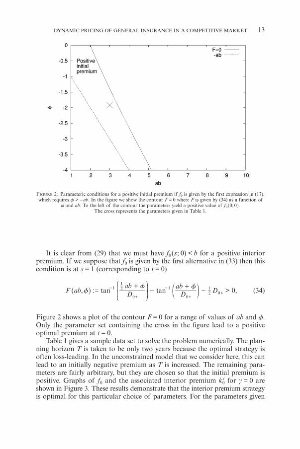
It is clear from (29) that we must have f0(s; 0) < b for a positive interiorpremium. If we suppose that f0 is given by the first alternative in (33) then thiscondition is at s = 1 (corresponding to t = 0)
, : > ,tan tanff f
F ab Dab
Dab
D 01
0
21
1
021
0=+
-+
--
+
-
++
J
L
KK^ d
N
P
OOh n (34)
Figure 2 shows a plot of the contour F = 0 for a range of values of ab and ƒ.Only the parameter set containing the cross in the figure lead to a positiveoptimal premium at t = 0.
Table 1 gives a sample data set to solve the problem numerically. The plan-ning horizon T is taken to be only two years because the optimal strategy isoften loss-leading. In the unconstrained model that we consider here, this canlead to an initially negative premium as T is increased. The remaining para-meters are fairly arbitrary, but they are chosen so that the initial premium ispositive. Graphs of f0 and the associated interior premium k0
i for g = 0 areshown in Figure 3. These results demonstrate that the interior premium strategyis optimal for this particular choice of parameters. For the parameters given
DYNAMIC PRICING OF GENERAL INSURANCE IN A COMPETITIVE MARKET 13
FIGURE 2: Parameteric conditions for a positive initial premium if f0 is given by the first expression in (17),which requires ƒ > – ab. In the figure we show the contour F = 0 where F is given by (34) as a function of
ƒ and ab. To the left of the contour the parameters yield a positive value of f0(0; 0).The cross represents the parameters given in Table 1.
9784-07_Astin37/1_01 30-05-2007 13:52 Pagina 13

in Table 1 the first of the alternatives for f0 is applicable. From (20) there isblowup if
/, ,
tans D
A Dp 20 1b
0
10 0 !=
-
+
-
+^ h6 @
and then f0(sb) = ∞. For these parameter sets the value function is infinite andit is possible to generate infinite wealth.
We adopt a simple explicit finite difference scheme to solve (31) with a firstorder time difference and second order spatial differences (Smith 1985). Con-sequently, there is a restriction on how large the time step can be in order tomaintain numerical stability. In the computations, the nondimensional timestep was taken as Ds = 10–3 and the spatial step was taken as Dg = 10–2 unlessstated otherwise. The results for the parameters in Table 1 are shown in Fig-ure 4. Figure 4(a) shows the variation of the value function V through (24) withthe current state gt = g. The largest value function occurs when s = 0 and theloss ratio is g = 0 corresponding to, say, an infinite market average premium.From (29) and the boundary conditions (32) the interior relative premium islinear in g at termination s = 0 and on g = b = 1, ki = b = 1 for this particulardata set (see Figure 4(b)).
14 P. EMMS
FIGURE 3: Optimal dynamic premium strategy for constant loss ratio g = 0 as a function of the time totermination s using the parameters in Table 1. The expression for f0 is given by the first alternative in (33)
and the approximate relative strategy is given by (23).
9784-07_Astin37/1_01 30-05-2007 13:52 Pagina 14
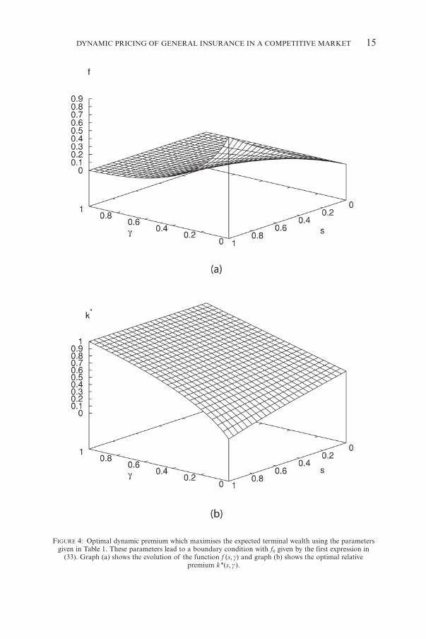
DYNAMIC PRICING OF GENERAL INSURANCE IN A COMPETITIVE MARKET 15
FIGURE 4: Optimal dynamic premium which maximises the expected terminal wealth using the parametersgiven in Table 1. These parameters lead to a boundary condition with f0 given by the first expression in
(33). Graph (a) shows the evolution of the function f (s, g) and graph (b) shows the optimal relativepremium k*(s, g ).
9784-07_Astin37/1_01 30-05-2007 13:52 Pagina 15

Suppose the finite difference grid is indexed by the points {( i, j ) | i = 0,1,…,Ns ;j = 0,1,…, Ng} where Ns, Ng are the number of time and spatial steps respec-tively. We adopt a fixed time step Ds = 1/Ns and a fixed spatial step Dg = b /Ng
and on the grid we write fij = f (iDs, jDg). We can assess the convergence ofthe finite difference scheme by defining
s g
,fN N
f1 1
1
,ij
i j
=+ +
!^ _h i
which measures the size of f over the domain and
dg = (Ds2 + Dg2)1/2,
which measures the resolution of the grid. In Figure 6 we plot || f || against dgusing the grid refinement Ns = 10k, Ng = 2000k with k = 1,2,…,50 and theparameters in Table 1. It is clear that the scheme is converging to || f || ∼ 0.104as dg → 0 with a linear convergence rate as one might expect given that weadopt a first order difference for the time step.
The optimal relative premium in Figure 4(b) gradually increases over theplanning horizon and this increase is greatest when the loss ratio g = 0. As g =p /p decreases so the breakeven premium becomes much less than the marketaverage premium p. This means the insurance market is overpricing insuranceand so there is greater scope to undercut the market price and still generatedemand. This strategy leads to large market exposure through the demand lawand large profits as can be seen in Figure 4(a) since as f increases so does thevalue function V. The form of the premium strategy is strongly influenced bythe qualitative features of the boundary condition on g = 0 given by (33). Asthe point of blow-up sb nears the domain [0,1] so the values of f0 become verylarge, which leads to negative values of k0. If k < g then this is a loss-leadingstrategy so one can identify the first form of (33) as of loss-leading type pro-viding the time horizon is sufficiently large.
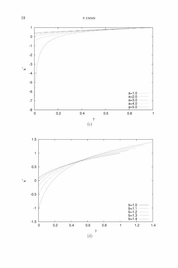
We study the sensitivity of the model by varying the parameters r, s2, a, b,and ƒ in turn in Figures 5(a)-(e). The plots show the optimal relative premiumk* at t = 0 given the current state variable g. The optimal strategy is fairly insen-sitive to the mean reversion, r, and the volatility of the loss ratio, s2. The expectedvalue of the loss-ratio tends to one as r gets large so that there are few oppor-tunities for loss-leading and it is optimal to set a higher premium as shown inFigure 5(a). If the volatility is large and the current loss-ratio g is small thenthe loss ratio may substantially increase over the time horizon, so that it isoptimal to set a higher premium and diminish loss-leading. Conversely, if thevolatility and the current loss-ratio g are large then there is the possibility thatthe loss-ratio will substantially decrease over the planning horizon and loss-leading opportunities will become available. This lowers the optimal premiumas seen in Figure 5(b).
16 P. EMMS
9784-07_Astin37/1_01 30-05-2007 13:52 Pagina 16

DYNAMIC PRICING OF GENERAL INSURANCE IN A COMPETITIVE MARKET 17
9784-07_Astin37/1_01 30-05-2007 13:52 Pagina 17
18 P. EMMS
9784-07_Astin37/1_01 30-05-2007 13:52 Pagina 18

The optimal strategy is strongly dependent on the form of the demand func-tion (parameters a and b) and the parameter ƒ as shown in Figures 5(c)-(e).As a or b is increased the demand for insurance is larger for a fixed relative pre-mium. This favours a loss-leading strategy because lowering the premium gen-erates considerable exposure. Ultimately this leads to negative initial premiumvalues as shown in Figure 5(c),(d) because there is no borrowing constraint inthe model. The parameter ƒ encompasses the drift in the market average pre-mium and the policy length: large growth and long policies tend to increase ƒ,which increases the magnitude of loss-leading and leads to negative initial pre-mium values. If the market average premium grows rapidly whilst the breakevenpremium is fixed this again favours loss-leading.
4. TOTAL DISCOUNTED UTILITY OF WEALTH
It is not clear that the objective of maximising the expected terminal wealthis the most appropriate goal for an insurer. Insurance companies must have
DYNAMIC PRICING OF GENERAL INSURANCE IN A COMPETITIVE MARKET 19
FIGURE 5: Sensitivity of the optimal initial relative premium k*(g,1) to (a) the loss ratio mean reversion r,(b) the loss ratio volatility s2 (Ds = 10–5), (c) the demand parameter a, (d) the demand parameter b,
and (e) the parameter ƒ. The objective is to maximise the expected terminal wealth and theremaining data is taken from Table 1.
9784-07_Astin37/1_01 30-05-2007 13:52 Pagina 19

sufficient funds to cover legal requirements and satisfy the demands of theirshareholders. If an insurer adopts a strategy which leads to large losses in theexpectation of significant income in the future then this generates substantialrisk. An alternative objective often used in financial applications of stochas-tic control theory is to maximise the expected total discounted utility of wealth:
tb
k,sup� e U dttT
0
- w# ^ h( 2
where U = U (wt) is the utility function and T = t / T. From such an objectiveone might expect a more conservative optimal strategy k* because initial loss-leading does affect the objective. For simplicity, we consider the exponentialutility function
U(w) =c1 (1 – e–cw) and c > 0.
This function has constant (absolute) risk aversion c and is a member of theHyperbolic Absolute Risk Aversion (HARA) family (Pratt 1964; Gerber &Pafumi 1998). Browne (1995) used this utility function to calculate the optimalinvestment strategy for an insurer. We adopt a utility function of this form sinceas c → 0, U → w so that the objective is linear in the wealth and it is easier tofind the solution to the Bellman equation.
The appropriate definition for the value function is
sb
k, ,sup�V x t e U ds xt
t
T= =
- s w X#^ ^h h( 2 (35)
and the corresponding Bellman equation is
Vt + mpVp + 21 s1
2 p2Vpp + g ( 21 s2
2 – r log g)Vg + 21 s2
2g2Vgg – kqVq – awVw +
qk
sup{G(k) (Vq + p(k – g )Vw)} +b
ce t-
(1 – e–cw) = 0, (36)
with boundary conditions
V (g = b, t ) = 0, V (x,T ) = 0.
The interior premium is given by (10), as before, since the control does not enterthe objective function in (35). Substituting the interior premium into the aboveequation yields
Vt + mpVp + 21 s1
2 p2Vpp + g ( 21 s2
2 – r log g)Vg + 21 s2
2g2Vgg +
q( 21 a(b – g) – k)Vq + (–aw + 4
1 apq(b – g)2)Vw +q
w
aqV4
2
Vp +b
ce t-
(1 – e–cw) = 0. (37)
20 P. EMMS
9784-07_Astin37/1_01 30-05-2007 13:53 Pagina 20

Again, we suppose that the first order condition does fulfill the maximisationoperation in the Bellman equation and that the value function is sufficientlysmooth that Ito’s lemma can be applied in deriving (36).
At termination t = T the optimal premium is undefined because the valuefunction is identically zero. This should be contrasted with the well-definedterminal optimal premium given by (11) for the terminal wealth case. However,near the end of the time horizon at t = T – dt where dt is a small time incre-ment we find by differencing the Bellman equation
VT – dt =b
ct ed T-
(1 – e–cw).
Therefore, Vq = 0 and the terminal optimal premium is identical to (11) asdt → 0 providing that the differencing is consistent with the spatial boundaryconditions.
We nondimensionalise the Bellman equation by using the scales in (30) sup-plemented by
p = [ p ] p̂ , q = [q ]q, w = [ p ] [q ]w, V = [ p ] [q ]T, b̂ = bT,
where [ p] and [q ] are scales derived from the value of the market average pre-mium and the exposure at t = 0. Let us introduce the parameter
e = c [ p ] [q ],
as a dimensionless measure of the risk aversion of the insurer. Henceforth weshall drop the hats on the nondimensional variables. The nondimensional Bell-man equation is therefore
Vs = mpVp + 21 s1
2 p2Vpp + g ( 21 s2
2 – r log g)Vg + 21 s2
2g2Vgg – kqVq – awVw +
qk
sup{G(k) (Vq + p(k – g)Vw)} +bee
s1- -] g
(1 – e – ew). (38)
We aim to solve this equation approximately using a perturbation expansionfor e % 1.
4.1. No Risk Aversion
If the insurer has no risk aversion then e = 0 (corresponding to c → 0) and theutility function is linear in the wealth process. We look for a solution of theform
V (x,s) = e–b (1 – s) (g(s)w + qph(g,s)). (39)
DYNAMIC PRICING OF GENERAL INSURANCE IN A COMPETITIVE MARKET 21
9784-07_Astin37/1_01 30-05-2007 13:53 Pagina 21

Substituting into (38) we obtain two equations for g and h:
g� + (a + b )g – 1 = 0, (40)
hs = g ( 21 s2
2 – r log g)hg + 21 s2
2g2hgg + k
sup{G(k) (h + (k – g)g)}, (41)
where the boundary conditions are derived in a similar way to the terminalwealth case and are
g(0) = 0, h(0,s) – h0(s) = h(b,s) = h(g,0) = 0. (42)
In terms of these functions the interior relative premium is
,k b
g sh s
gg
2
1i= + -
^
^f
h
hp (43)
and when the control is interior the equation for h becomes
hs = g ( 21 s2
2 – r log g)hg + 21 s2
2g2hgg + C(s)h2 + D (g)h + E (g,s), (44)
where
C (s) =g sa
4 ^ h,
D (g) = 21 a (b – g) + m – b – k,
E (g,s) = 41 a (b – g)2g(s).
The equation for g can be integrated immediately to give
g(s) =a b
1+
(1 – e– (a + b )s), (45)
and, as before, the function h0 is given by the solution to the problem indepen-dent of g :
dsdh0 = C(s)h0
2 + D(0)h0 + E (0, s),
with terminal condition h0(0) = 0. This is a Riccati equation for which there isno general technique for obtaining a solution. Moreover, these equationscan exhibit spontaneous singularities for finite s: this phenomenon restricts theparameter range over which the control will be smooth in a similar way to (17).
In order to determine how the relative premium differs from Section 3 we set
F (g,s) =,
g sh sg^
^
h
h,
22 P. EMMS
9784-07_Astin37/1_01 30-05-2007 13:53 Pagina 22

so that (29) and (43) have the same form. After some manipulation (44) becomes
Fs = g ( 21 s2
2 – r log g)Fg + 21 s2
2g2Fgg + 41 aF 2 + A
g sg
1-^
^d h
hn F + B (g). (46)
Notice there is an extra term –F /g on the RHS of this equation comparedwith (27). Since g(s) is a non-negative function and we expect F is positive asbefore, the gradient Fs is reduced and so –F is increased as the time to termi-nation, s, is increased. Therefore, in comparison with the terminal wealth case,the optimal relative premium is larger and the strategy is more conservative.If the discount rate b is made larger then g decreases and so F is made smaller.This in turn makes –F larger and therefore increases the interior premium ki.
We can reduce the free parameter set by writing
h = a + b. (47)
Thus the nondimensional free parameters are r, s2, a, b, ƒ, h: these parame-ters and the current state, x, determine the optimal relative premium. We havean additional free parameter over the terminal wealth case because we haveintroduced the discount factor b.
Again, an explicit finite difference scheme is used to solve equation (41) withthe boundary conditions in (42) using the grid Ds = 10–4, Dg = 10–2. Figure 7
DYNAMIC PRICING OF GENERAL INSURANCE IN A COMPETITIVE MARKET 23
FIGURE 6: Convergence of the finite difference scheme as the mesh is refined. The resolution of the meshis proportional to dg while || f || is the average value of f over the domain.
9784-07_Astin37/1_01 30-05-2007 13:53 Pagina 23

24 P. EMMS
FIGURE 7: Optimal dynamic premium which maximises the total discounted utility of wealth using theparameters given in Table 1 with a linear utility function. Graph (a) shows the evolution of the function
h (s,g) and graph (b) shows the optimal relative premium k*(s, g).
9784-07_Astin37/1_01 30-05-2007 13:53 Pagina 24

shows plots of h(g,s) and k*(g,s) for the sample data set in Table 1. The opti-mal strategy is qualitatively similar to the terminal wealth case although theoptimal relative premium is larger. The optimal premium strategy is moreconservative here because loss-leading affects the total utility of wealth of theinsurer. The robustness of the control with respect to the objective gives usconfidence that the analytical control in (14) is an appropriate strategy toconsider for an insurer. The sensitivity of the optimal control to the modelparameters is similar to the terminal wealth case and so this is not shown.
4.2. Weakly Nonlinear Utility Function
We consider a nonlinear objective by including the next term in an asymptoticexpansion for the utility function
U(w) a w –21
ew2, (48)
where we assume w a O (1) by the choice of scaling.We use a perturbation expansion for V in terms of e % 1 to yield a succes-
sion of linear systems. Thus we write
V a V0 + eV1 + …
k* a k0* + ek1
* + …
Substituting into (38) and assuming an interior control, V0 is given by (39) whileat O (e) we find
V1s = mpV1p + 21 s1
2 p2V1pp + g ( 21 s2
2 – r log g)V1g + 21 s2
2 g2V1gg +
q( 21 a (b – g) – k)V1q + (–aw + 4
1 apq (b – g)2)V1w +
q1w1,
g taqh t
V hg t
g p4
2 21
- -V
^
^
^e
h
h
ho e– b (1 – s) w2, (49)
and
V1(g = b,s) = 0, V1(x,0) = 0.
This is a linear PDE with four space dimensions. The value function V1 is notlinear in each of the state variables because of the last term in the equation.
We aim to reduce the dimension of the problem by looking for a solutionof the form
V1(x,s) = e– b (1 – s) (m (g,s)p2q2 + n(g,s)pqw + r(s)w2). (50)
DYNAMIC PRICING OF GENERAL INSURANCE IN A COMPETITIVE MARKET 25
9784-07_Astin37/1_01 30-05-2007 13:53 Pagina 25

Substituting (50) into (49) and collecting together the O(1), O(w) and O(w2)terms yields three equations for m, n and r:
ms = g ( 21 s2
2 – r log g)mg + 21 s2
2 g2 mgg +
2,f aa b g
ah m a bgh ng h s g2 41
22
2
- + - - + + + - -J
L
KK^d ^
N
P
OOh n h
ns = g ( 21 s2
2 – r log g)ng + 21 s2
2 g2 ngg +
2,f aa b g
ah n a bgh rg h g2 22
12
2
- + - - + + - -J
L
KK^d ^
N
P
OOh n h
,adsdr rb2 2
1= - + -^ h (51)
with boundary conditions
m(0,s) – m0(s) = m(b,s) = m(g,0) = 0,
n(0,s) – n0(s) = n(b,s) = n(g,0) = 0,
r(0) = 0,
and where g = g(s) and h = h(g,s) are given by (41) and (45). The boundary func-tions m0(s) and n0(s) satisfy the coupled ODEs:
2
2
,
,
f a
f a
dsdm
ab gah
m a bg
hn
dsdn
ab gah
n a bg
hr
h s
h
2 4
2 2
012 0
02
2
0
021 0
02
2
= + - - + + + -
= + - - + + -
0
0
J
L
KK
J
L
KK
e
e
N
P
OO
N
P
OO
o
o
with initial conditions m0(0) = n0(0) = 0. On integrating (51) and applying theboundary condition we obtain
s
.a
r s eb2 2
1a b2
=+
-- +
^^
]
hh
g
From (10) the leading-order interior relative premium is given by (43) whilstthe second-order term is
w1
w w
q
0 0
1*
,, , , .
k
s sh s
qn s r s w q m s wn sg
g g gp p
2
21 2 2
q
q1
0
0= -
= + - -g g
VV
VV
VV
p f
^ ^
^^ ^_ ^ ^f
p
h h
hh h i h hp
26 P. EMMS
9784-07_Astin37/1_01 30-05-2007 13:54 Pagina 26

DYNAMIC PRICING OF GENERAL INSURANCE IN A COMPETITIVE MARKET 27
For a nonlinear objective function the optimal relative premium is a functionof all four state variables. This complicates the comparison of how the premiumstrategy changes if the insurer changes its objective. Also note that m (g,s)depends on the coefficient of volatility of the market average premium, s1, andconsequently so does the relative optimal premium.
Figure 8(a) and (b) show the solutions for m and n computed using anexplicit finite difference scheme and the parameters in Table 1. All of thefunctions m, n and r are negative over the domain of integration indicating thatrisk aversion decreases the value function V. The greatest decrease in V is att = g = 0 since that is where most wealth is generated. Figure 8(c) showsthe perturbation to the optimal relative premium if we set the current statevariables p / q / w / 1. Notice that k1* is positive for these processes, so thatincreasing the risk aversion increases the optimal relative premium. This increaseis greatest if the current loss ratio is small. Figure 9 shows the qualitative effectof increasing the insurer’s risk aversion e. Risk aversion leads to a more con-servative interior premium strategy – this generates less exposure over the plan-ning horizon, which decreases the total claims and maintains premium income.
5. CONCLUSIONS
We have found the optimal premium strategy for an insurer in a competitivemarket using optimal control theory. In general, the Bellman equation arisingfrom control theory contains a degenerate diffusion operator. For the currentmodel we have shown how this degeneracy can be removed by a change ofvariables, which makes the resulting problems easy to solve numerically. Thechoice of a linear demand function (in the relative premium) leads to a singlenonlinear term in the Bellman equation which considerably simplifies the analy-sis. Our ability to find the optimal premium strategy is limited by the valuesgiven to the model parameters. We have found the conditions that lead to a pos-itive initial premium for the terminal wealth case. In general, if the optimal con-trol is smooth then the optimal premium gradually increases over the term ofthe planning horizon for the parameter sets considered here. We find that asrisk aversion is increased so does the optimal relative premium strategy. Thisgenerates lower exposure and so ultimately lower overall wealth. The numeri-cal value of the terminal relative premium is identical for all the objectivesstudied here.
One significant assumption is that we can treat the market distinctly fromthe insurer so that whatever the insurer’s premium, the market does not reactwith a competitive price. Currently we are investigating how one might relax thisassumption by incorporating an adjustment term in the process followed by themarket average premium. Another modelling simplification is the specificationof a stochastic process for the breakeven premium. This premium representsthe cost of insurance for the insurer and assessment of this quantity requiresa good model for the claims process and an accurate definition of the loading
9784-07_Astin37/1_01 30-05-2007 13:54 Pagina 27

28 P. EMMS
9784-07_Astin37/1_01 30-05-2007 13:54 Pagina 28

DYNAMIC PRICING OF GENERAL INSURANCE IN A COMPETITIVE MARKET 29
Figure 8: Optimal premium strategy when the insurer maximises its expected total utility of wealth.The utility function is a quadratic function of the wealth w in (48) and represents the second order
expansion of an exponential utility function when risk aversion is small. Plots (a) and (b) show the solutionfor m (g,s ) and n (g,s ) for the parameters in Table 1, while (c) shows the deviation in the interior relative
premium k*1 (g,s ) for p = q = w = 1.
FIGURE 9: Qualitative comparison of the optimal premium strategy p* if the loss-ratio is constant and themarket average premium is constant for the objective of either maximising expected terminal wealth ortotal discounted utility of wealth with a linear utility function. The loss ratio in the diagram is g = 1/2
so the terminal optimal premium is p*T = † p (b + † ).
9784-07_Astin37/1_01 30-05-2007 13:54 Pagina 29

factor. The benefit of using this process to define a loss-ratio is that the wealthprocess wt directly reflects the current wealth of the insurer including its liabili-ties.
Sample paths have been restricted to prevent the insurer leaving and the re-entering the insurance market. If one relaxes this assumption then one mustcope with the non-differentiability of the demand function (9) at k = b and thedetermination of when the insurer should stop selling insurance. We have intro-duced this non-differentiability in order that the feedback control is tractable.However, it is not clear that there is a classical solution to the Bellman equationfor the more general problem and so one cannot apply a verification theoremto ensure optimality of the feedback control. The problem is reminiscent of theAmerican option pricing problem posed as an optimal control problem fromwhich one obtains a semi-linear Black-Scholes equation with a discontinuouscash flow. Benth, Karlson & Reikvam (2003) have determined simple numericalschemes using viscosity solutions of the Black-Scholes equation (Fleming &Soner 1993). For these schemes it is not required to track the free boundaryrepresenting when it is optimal to exercise the option: its position is givenimplicitly from the numerical solution. It is tempting to suggest that a similarconstruction might be applied to the competitive pricing problem when theinsurer is permitted to have periods of no sales.
The difficulty with using dynamic programming to calculate an optimalpremium strategy lies with the balance between posing a realistic model and theability to solve and interpret the resulting high-dimensional Bellman equation.We have found an analytical solution for a restricted case, and shown that thenumerical solution of the more general problem is feasible, even for a quitesophisticated objective function. Often the premium that the insurer can set is con-strained by both legislation and the desire to minimise the risk of loss-leading.The incorporation of constraints into the optimal control problem is anotherarea of ongoing research.
ACKNOWLEDGEMENTS
We gratefully acknowledge the financial support of the EPSRC under grantGR/S23056/01 and the Actuarial Research Club of the Cass Business School,City University.
APPENDIX
A. MEAN CLAIM SIZE RATE PROCESS
If we drop the assumption that the evolution of the breakeven premium canbe deduced from policy data then we must deal directly with the mean claimsize rate (and related claims expenses) ut. This is, for example, the average sizeof claims received in one day per unit of exposure. It must be measured per
30 P. EMMS
9784-07_Astin37/1_01 30-05-2007 13:54 Pagina 30

unit time because it incorporates the intensity of claims as well as their mag-nitude. An appropriate wealth process is now given by
dwt = – awt dt + ptbtdt – utqt dt.
As before, the new and renewed business generates wealth ptbtdt in time dt whileclaims are now accounted for as they arise so that the loss of wealth is utqt dt.
In order to calculate a simple expression for the liabilities, it is convenientto adopt separate processes for the market average premium and the mean claimsize rate. We suppose that the market average premium reverts to current costof insurance in the long term and that the mean claim size rate is lognormallydistributed:
dpt = l (jut – pt) dt + m1pt dt + s1pt d W1t , (52)
dut = ut(m2 dt + s2d W2t) , (53)
where the mean reversion rate is l. The drifts m1, m2 and coefficients of volatilitys1, s2 are taken as constants. The current cost of insurance per unit exposurefor the whole market is
js ,� ds uX tt
t
t
t=
+
u#< F
where t is the length of policies, the current state of the system is Xt = (pt, ut,qt, wt) and
.ej m
1m
2=
-t2J
L
KK
N
P
OO
If no more insurance is sold at time t then the outstanding claims generate aloss of wealth for the insurer equal to
s s dsu qt
3
# ,
and the exposure decays exponentially according to (5):
qs = qte–k (s – t),
for s ≥ t. The expected liabilities of the insurer at the end of the time horizonis therefore
s .� q e e dsq u
u X k mTT s
TT
T Tk k
2
=-
3-#= G
We must have k > m2 otherwise the outstanding liabilities are infinite.
DYNAMIC PRICING OF GENERAL INSURANCE IN A COMPETITIVE MARKET 31
9784-07_Astin37/1_01 30-05-2007 13:55 Pagina 31
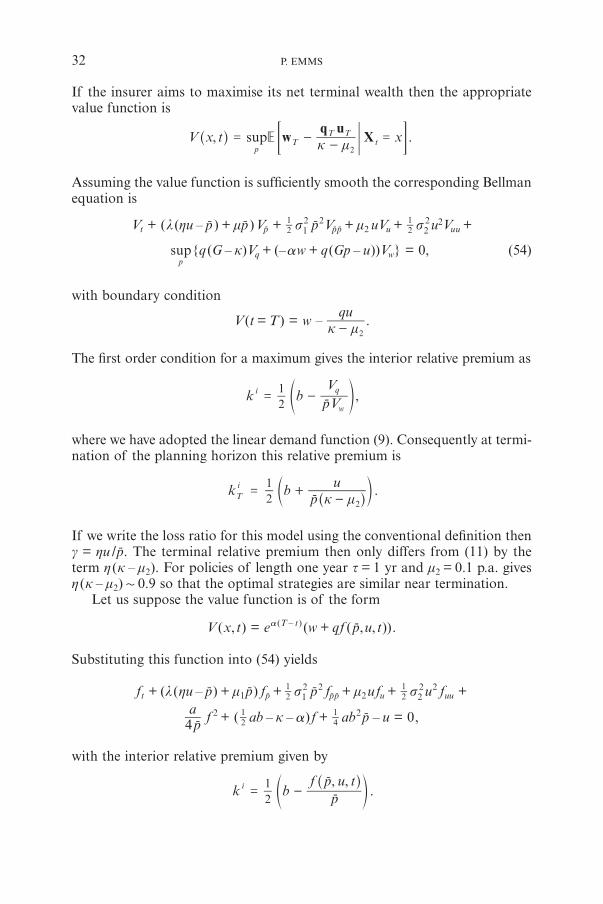
If the insurer aims to maximise its net terminal wealth then the appropriatevalue function is
p, .sup�V x t xw
q uXk mT
T Tt
2
= --
=^ h = G
Assuming the value function is sufficiently smooth the corresponding Bellmanequation is
Vt + (l (ju – p ) + mp )Vp + 21 s1
2 p2Vpp + m2 uVu + 21 s2
2u2Vuu +
psup{q (G – k)Vq + (–aw + q(Gp – u))Vw} = 0, (54)
with boundary condition
V(t = T ) = w –qu
k m2-.
The first order condition for a maximum gives the interior relative premium as
w
q ,k b p21i
= - VV
f p
where we have adopted the linear demand function (9). Consequently at termi-nation of the planning horizon this relative premium is
.k b uk mp2
1Ti
2= +
-^d
hn
If we write the loss ratio for this model using the conventional definition theng = ju /p. The terminal relative premium then only differs from (11) by theterm j (k – m2). For policies of length one year t = 1 yr and m2 = 0.1 p.a. givesj (k – m2) + 0.9 so that the optimal strategies are similar near termination.
Let us suppose the value function is of the form
V (x, t) = ea (T – t ) (w + qf (p,u, t)).
Substituting this function into (54) yields
ft + (l (ju – p) + m1p) fp + 21 s1
2 p2 fpp + m2ufu + 21 s2
2u2 fuu +
4ap f 2 + ( 2
1 ab – k – a) f + 41 ab2p – u = 0,
with the interior relative premium given by
, ,.k b
f u tp
p21i
= -^
fhp
32 P. EMMS
9784-07_Astin37/1_01 30-05-2007 13:55 Pagina 32

DYNAMIC PRICING OF GENERAL INSURANCE IN A COMPETITIVE MARKET 33
The function f is not linear in p or u because of the quadratic term in f so itappears as though we must solve this equation numerically. Consequently,rather than present a premium strategy as a function of three independentvariables (t, p and u), we have chosen in the main body of the paper to modelthe breakeven premium directly, which yields a strategy which is simpler tointerpret. However, the mean claim size rate model does have the merit ofexplicitly accounting for the risk in holding an exposure qt, and therefore maybe a suitable model for studying the optimisation problem when there are con-trol and state constraints.
If we drop (52) and explicitly relate the market average premium pt to themean claim size rate ut then the model only contains a single factor W2t. In thiscase analytical solutions similar to (17) can be found.
REFERENCES
ASMUSSEN, S. and TAKSAR, M. (1997) Controlled diffusion models for optimal dividend pay-out.Insurance: Mathematics and Economics, 20, 1-15.
BENTH, F.E., KARLSEN, K.H. and REIKVAM, K. (2003) A semilinear Black and Scholes partialdifferential equation for valuing American options. Finance and Stochastics, 7, 277-298.
BRITTON, N.F. (1986) Reaction-Diffusion Equations and Their Applications to Biology. AcademicPress.
BROWNE, S. (1995) Optimal investment policies for a firm with a random risk process: Expo-nential utility and minimizing the probability of ruin. Math. Oper. Res., 20, 937-958.
CAMPBELL, J.Y. and VICEIRA, L.M. (2001) Strategic Asset Allocation: Portfolio Choice for Long-Term Investors. New York: Oxford University Press.
DAYKIN, C.D. and HEY, G.B. (1990) Managing Uncertainty in a General Insurance Company.Journal of the Insitute of Actuaries, 117(2), 173-277.
DAYKIN, C.D., PENTIKÄINEN, T. and PESONEN, M. (1994) Practical Risk Theory for Actuaries.Chapman and Hall.
EMMS, P. and HABERMAN, S. (2005) Pricing general insurance using optimal control theory. AstinBulletin, 35(2), 427-453.
EMMS, P., HABERMAN, S. and SAVOULLI, I. (2007) Optimal strategies for pricing general insurance.Insurance: Mathematics & Economics, 40(1), 15-34.
FLEMING, W. and RISHEL, R. (1975) Deterministic and Stochastic Optimal Control. New York:Springer Verlag.
FLEMING, W.H. and SONER, H.M. (1993) Controlled Markov Processes and Viscosity Solutions.Springer-Verlag.
FRIEDMAN, A. (1964) Partial Differential Equations of Parabolic type. Prentice-Hall.GERBER, H.U. and PAFUMI, G. (1998) Utility Functions: From Risk Theory to Finance. North
American Actuarial Journal, 2(3), 74-100.HIPP, C. (2004) Stochastic Control with Application in Insurance. Working Paper, Universität Karls-
ruhe, Germany.HIPP, C. and PLUM, M. (2000) Optimal Investment for Insurers. Insurance: Mathematics and Eco-
nomics, 27, 215-228.HØJGAARD, B. and TAKSAR, M. (1997) Optimal Proportional Reinsurance Policies for Diffusion
Models. Scand. Actuarial J., 2, 166-180.KARATZAS, I. and SHREVE, S.E. (1998) Methods of Mathematical Finance. Springer.KOLMANOVSKII, V.B. and SHAIKHET, L.E. (1996) Control of Systems with Aftereffect. Transla-
tions of Mathematical Monographs, vol. 157. Americal Mathematical Society.LILIEN, G.L. and KOTLER, P. (1983) Marketing Decision Making. Harper & Row.MERTON, R.C. (1971) Optimum Consumption and Portfolio Rules in a Continuous Time Model.
Journal of Economic Theory, 3, 373-413.
9784-07_Astin37/1_01 30-05-2007 13:55 Pagina 33
MERTON, R.C. (1990) Continuous-time Finance. Blackwell.MURRAY, J.D. (2002) Mathematical Biology. Springer.PENTIKÄINEN, T. (1986) Discussion of “Underwriting strategy in a competitive insurance envi-
ronment”. Insurance: Mathematics and Economics, 5, 81-83.PRATT, J.W. (1964) Risk Aversion in the Small and in the Large. Econometrica, 32, 122-136.SAMUELSON, P.A. (1969) Lifetime Portfolio Selection by Dynamic Stochastic Programming. Review
of Economics and Statistics, 51, 239-246.SMITH, G.D. (1985) Numerical Solution of Partial Differential Equations: Finite Difference Methods.
Oxford University Press.Taylor, G.C. (1986) Underwriting strategy in a competitive insurance environment. Insurance:
Mathematics and Economics, 5(1), 59-77.
PAUL EMMS
Faculty of Actuarial Science and InsuranceCass Business SchoolCity University, London
34 P. EMMS
9784-07_Astin37/1_01 30-05-2007 13:55 Pagina 34