Pricing discretion and price regulation in competitive industries

Alberto Iozzi, Roberta Sestini, Edilio Valentini

CEIS Tor Vergata - Research Paper Series, Vol. 23, No. 69, January 2005

This paper can be downloaded without charge from the Social Science Research Network Electronic Paper Collection:

http://papers.ssrn.com/abstract=695282

CEIS Tor Vergata

RESEARCH PAPER SERIES

Working Paper No. 69 January 2005

Pricing discretion and price regulation

in competitive industries∗

Alberto Iozzi†

Universita di Roma “Tor Vergata” and

University of Leicester

Roberta Sestini‡

Universita di Roma “La Sapienza”

Edilio Valentini§

Universita “G. D’Annunzio” di Chieti-Pescara

March 17, 2005

∗The authors wish to thank Nicola Rossi and Carla Pace for their contributions in the early

stages of this project, and Per J. Agrell, Gianni De Fraja, Massimo Roma, Carlo Scarpa, and

seminar audience at the University of Padua for their useful comments†Universita di Roma “Tor Vergata”, Dip. SEFEMEQ, Via Columbia 2, I-00133 Rome, Italy.

E-mail: alberto.iozzi@uniroma2.it‡Universita di Roma “La Sapienza”, Dip. di Informatica e Sistemistica “A. Ruberti”, Via

Buonarroti 12, I-00185 Rome, Italy. E-mail: sestini@dis.uniroma1.it§Universita “G. D’Annunzio” di Chieti-Pescara, Dip. di Economia e Storia del Territorio,

Viale Pindaro 42, I-65127 Pescara, Italy. E-mail: valentin@unich.it

Pricing discretion and price regulation in competitive industries

Alberto Iozzi

Roberta Sestini

Edilio Valentini

Abstract

Price capped firms enjoy a large degree of pricing discretion, which may damage

captive customers and have adverse effects on the development of competition

when regulated firms also operate in competitive industries. We study two alter-

native regulatory approaches to limit such a discretion. The first one places a fixed

upper limit to the prices charged in captive markets; the other constrains the cap-

tive prices relatively to the prices set in the more competitive markets. We refer

to the former approach as the Absolute regime, and to the latter as the Relative

regime. We analyse the effects on prices, competition, and welfare stemming from

the two regimes in a simple model where the regulated firm faces competition by

a competitive fringe in some of the markets it serves. We find that the Relative

regime is not much more effective in protecting captive customers since captive

prices may be identical under both regimes. Moreover, since it makes more costly

to the incumbent regulated firm to reduce its competitive price, this is weakly

higher than under the Absolute regime. However, this is also the reason why the

Relative regime turns out to be more pro-competitive: the total output supplied

by competitors and/or the number of firms entering the potentially competitive

market might be enhanced under this rule. The effects on aggregate welfare are

ambiguous. We provide some evidence that the Relative regime is more likely

to positively affect consumers’ surplus and social welfare the more efficient is the

competitive fringe.

JEL numbers: L13, L50.

Keywords: price regulation, pricing discretion, competition.

1 Introduction

Market power typically gives firms a large discretion over the level and the struc-

ture of their prices. The economic literature has always paid a close attention to

the effects of this discretionality and to the limits, if any, which should be placed

on it (see, for instance, Varian, 1989, and Armstrong and Vickers, 1991). This

paper studies this issues in the context of regulation of a firm operating in an

imperfectly competitive industry.

Economists and policy makers have by now agreed that price cap regulation

is a simple and efficient way to limit the firm’s discretionality over the level of

its prices; indeed, the price cap places an upper limit to the average level (or,

sometimes, to its dynamics) of the prices of all the goods offered by the firm in

markets where it has a large degree of market power (see the seminal paper by

Vogelsang and Finsinger, 1979, and the excellent book by Armstrong et al., 1994).

However, in practice regulators make also the effort to limit the discretionality of

the firm over its price structure. One typical instrument to pursue this objective is

the imposition of caps to the average level of prices of subsets of goods offered by

the firm (in regulators’ jargon, sub-baskets), possibly used in conjunction with a

comprehensive price cap. Clearly, the higher is the number of sub-baskets and the

smaller is the number of elements in each of them, the lower is the firm’s discretion

over its price structure. This approach, taken to the extreme, has often led regu-

lators to set limits to individual prices. For instance, in the telecommunications

industry, where in most countries the majority of consumers are still subscribers

of the dominant operator, a specific cap is typically imposed on the rental fee.

A different approach has been debated for the electricity industry in the UK,

where one of the options discussed in the occasion of the recent review of supply

price constraints was to set an upper limit to the ratio of the prices charged to

prepayment customers (thought to be not sufficiently protected by competition)

with respect to those charged to credit customers (i.e. those customers acting

in markets where competition is sufficiently developed). Despite this option was

1

eventually discarded, a similar constraint is now applied in the electricity distri-

bution price control where, in addition to a revenue cap, ”domestic prepayment

meters are [..] subject to a relative price cap limiting the extra charges for pre-

payment meters that can be made by DNOs [Distribution Network Operators] to

suppliers over and above the charges that are made for an equivalent domestic

credit meter” (Ofgem, 2003, p. 6). In Italy, a similar constraint is faced by motor-

way concessionaires which, together with a comprehensive price cap, are requested

to set peak prices up to a maximum ratio to their off peak prices.

All these approaches originate from the same regulators’ concern: the regu-

lated firm may find it profitable to fix particularly high prices in some markets by

setting at the same time low prices in some other markets. This may adversely

affect the aggregate consumers’ welfare and, if one has reasons to take care of

it, also its distribution across markets. It may also have undesired effects on the

development of competition, if the firm uses its pricing freedom to price aggres-

sively in (potentially) competitive markets (Armstrong and Vickers, 1993; Otero

and Waddams, 2002).

Hence the open question is on the nature of the limits (if any) that should

be imposed on the discretionality granted to the regulated firm over its price

structure. While a number of studies have examined this issue in monopolistic

industries (Armstrong and Vickers, 1991 and 2000; Ireland, 1992; Armstrong and

Sappington, forthcoming), little attention has been devoted to the analysis of

the possible implications of the limits to the pricing discretion of a dominant

firm in an imperfectly competitive environment. To our knowledge, this issue

is first tackled in Armstrong and Vickers (1993) who analyse, in a two-market

setting, the effects of different policies towards price discrimination by a dominant

firm that faces potential competition in one of the markets it serves, with and

without price cap regulation. They show that entry is weakly more likely when

the pricing discretion by the dominant firm is constrained by a ban on price

discrimination and when the firm faces independent caps in the two markets;

2

both these policies have nevertheless ambiguous effects on welfare. More recently,

Anton et al. (2002) focus on the issue of cross-market restrictions associated with

universal service provisions. In a two-market setting – one captive, one where two

firms interact strategically –, they find that these cross-market restrictions are at

the disadvantage of the firm supplying both markets.1

This paper compares different approaches for limiting the pricing discretion

of a regulated firm, both in terms of fostering competition and maximising social

welfare, which are usually the primary objectives of regulators. Following Arm-

strong et al. (1996), we present a stylized model of an industry where there is a

regulated firm offering two goods and a fringe of unregulated price-taker potential

competitors, offering a good which is a substitute of one of the goods supplied

by the regulated firm. We analyse two regulatory regimes that constrain only the

pricing choices of the incumbent firm. Both regimes include a price cap on the

average level of its prices. Moreover, one of the two regimes – referred to as the

Absolute regime – places a fixed upper limit to the price charged in the monopo-

listic market; the other regime – defined as the Relative regime – places instead a

limit on the captive price relatively to the price charged in the competitive market,

i.e. it constrains the ratio of the two prices.

We study the effects of these two regulatory regimes upon equilibrium prices,

the development and extent of competition, and social welfare. We find that the

Relative regime is not much more effective than the Absolute regime in protect-

ing captive customers, since captive prices may be identical under both regimes.

However, the Relative regime makes more costly to the regulated firm to reduce

its competitive price, since this eventual action is coupled with a reduction of

the monopolistic price: hence, the competitive price is generally higher under the

Relative regime. This introduces the other relevant difference between the two

regimes: the Relative regime is generally more able to foster competition, as it1The effects of price cap regulation on competition are also studied by Bos and Nett (1990),

Iozzi (2001) and Iozzi and Fioramanti (2004).

3

may induce a larger (aggregate) supply by the competitor(s). The welfare ranking

of the two regimes cannot be generally established. In a linear example, we find

that under the Relative regime captive customers are not necessarily better off,

while competitive customers are generally worse off than under the alternative rule.

In this example, the Relative regime is more likely to positively affect consumers’

surplus and social welfare the more efficient is the competitive fringe. Although

this conclusion does not fully address the issue of efficiency of entry2, it provides

some evidence of the importance of the relative efficiency of the competing firms

in determining the welfare properties of the regimes under analysis.

The paper is organised as follows. Section 2 illustrates the model. Section 3

provides some general results on equilibrium prices set by the regulated firm and

on the equilibrium behavior by the competitor(s) under the two regimes. Section 4

illustrates these results in a simplified framework, where market demand is linear

and products are homogeneous. Within this example, some welfare comparisons

of two schemes are shown. Section 5 concludes with some final remarks.

2 The model

We consider an industry where a firm, denoted with M , produces two goods, x1

and x2. The market for x1 is captive to firm M , possibly because of legal con-

straints or (market specific) prohibitively high sunk costs. There is a competitive

fringe of N (with N sufficiently large) price-taking firms, all potentially willing to

supply another good, X2, which is a substitute of x2. In the rest of the paper, we

will sometimes refer to good x1 and x2 as captive (or monopoly) and competitive

good respectively. While the hypothesis of price-taking behaviour is introduced to

sidestep any issue of market power of the competitors, the different nature of the

two markets is meant to represent the different speed at which, in many utilities

industries, competition has developed in different markets of the same industry.

Let pi denote firm M ’s prices for xi, where i = 1, 2, and let P2 be the price2A thorough discussion of this issue can be found in Vickers (2004).

4

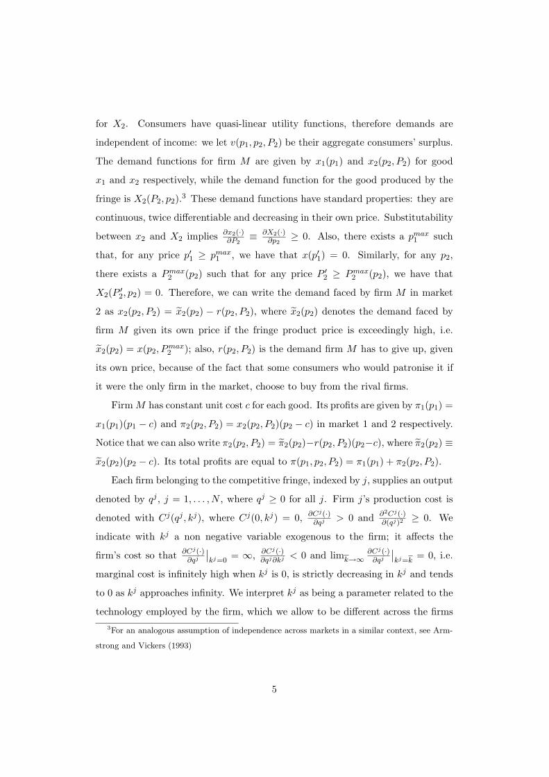
for X2. Consumers have quasi-linear utility functions, therefore demands are

independent of income: we let v(p1, p2, P2) be their aggregate consumers’ surplus.

The demand functions for firm M are given by x1(p1) and x2(p2, P2) for good

x1 and x2 respectively, while the demand function for the good produced by the

fringe is X2(P2, p2).3 These demand functions have standard properties: they are

continuous, twice differentiable and decreasing in their own price. Substitutability

between x2 and X2 implies ∂x2(·)∂P2

≡ ∂X2(·)∂p2

≥ 0. Also, there exists a pmax1 such

that, for any price p′1 ≥ pmax1 , we have that x(p′1) = 0. Similarly, for any p2,

there exists a Pmax2 (p2) such that for any price P ′

2 ≥ Pmax2 (p2), we have that

X2(P ′2, p2) = 0. Therefore, we can write the demand faced by firm M in market

2 as x2(p2, P2) = x2(p2) − r(p2, P2), where x2(p2) denotes the demand faced by

firm M given its own price if the fringe product price is exceedingly high, i.e.

x2(p2) = x(p2, Pmax2 ); also, r(p2, P2) is the demand firm M has to give up, given

its own price, because of the fact that some consumers who would patronise it if

it were the only firm in the market, choose to buy from the rival firms.

Firm M has constant unit cost c for each good. Its profits are given by π1(p1) =

x1(p1)(p1 − c) and π2(p2, P2) = x2(p2, P2)(p2 − c) in market 1 and 2 respectively.

Notice that we can also write π2(p2, P2) = π2(p2)−r(p2, P2)(p2−c), where π2(p2) ≡x2(p2)(p2 − c). Its total profits are equal to π(p1, p2, P2) = π1(p1) + π2(p2, P2).

Each firm belonging to the competitive fringe, indexed by j, supplies an output

denoted by qj , j = 1, . . . , N , where qj ≥ 0 for all j. Firm j’s production cost is

denoted with Cj(qj , kj), where Cj(0, kj) = 0, ∂Cj(·)∂qj > 0 and ∂2Cj(·)

∂(qj)2≥ 0. We

indicate with kj a non negative variable exogenous to the firm; it affects the

firm’s cost so that ∂Cj(·)∂qj

∣∣kj=0

= ∞, ∂Cj(·)∂qj∂kj < 0 and limk→∞

∂Cj(·)∂qj

∣∣kj=k

= 0, i.e.

marginal cost is infinitely high when kj is 0, is strictly decreasing in kj and tends

to 0 as kj approaches infinity. We interpret kj as being a parameter related to the

technology employed by the firm, which we allow to be different across the firms3For an analogous assumption of independence across markets in a similar context, see Arm-

strong and Vickers (1993)

5

in the fringe: the larger is kj the better are the technological conditions for firm

j. Another possible interpretation is with kj representing the institutional and/or

regulatory framework within which the firm competes with the regulated firm.

For example, kj could reflect different interconnection and number portability

rules, the existence of switching costs, etc., which of course affect the firm’s cost

(and supply function). These factors may have a different effect on the firm’s

behaviour according to the technology chosen: for instance, in the TLC industry,

ULL rules only influence the behaviour of carrier selection or carrier pre-selection

operators but not that of cable operators. Hence, the possibility, also under this

interpretation, of different kj ’s for the different firms in the fringe.

Firm j’s profits are denoted by θj(P2, kj) = P2q

j − Cj(qj , kj). By Hotelling’s

lemma, ∂θj(·)∂P2

= sj(P2, kj), where sj(P2, k

j) is firm j’s supply function, which is

weakly increasing in P2. The hypothesis on the relationship between the firm’s

cost and the parameter kj ensures that ∂sj(P2,kj)∂kj > 0.

We follow Armstrong et al. (1996) and treat the fringe as if it were a single

price taking firm, say firm E. This firm chooses its total output by solving the

following nested optimisation problem

θ(P2,k) ≡ maxq≥0

P2q −min

qj

∑

j

Cj(qj , kj)|∑

j

qj = q

(1)

where q =∑

j qj is the aggregate quantity supplied and k = (k1, . . . , kN ) is the

N -dimensional vector of the kj parameters for the N firms in the fringe. By

Hotelling’s lemma, ∂θ(P2,k)∂P2

= s(P2,k) where s(·) is the firm E’s supply function,

which is increasing in P2. Similarly to the case of individual firms, for any two N -

dimensional vectors k = (k1, . . . , kN ) and k = (k1, . . . , kN ) such that 0 ≤ kj ≤ kj

for all j = 1, . . . , N and kj < kj for at least one j, we have that s(P2,k) ≤s(P2,k). To save notation, in the rest of the paper, for any two vectors having

this relationship each other, we will say that 0 ¹ k ≺ k.

Our analysis focuses on two regulatory regimes that, as it is common in prac-

tice, only constrain the prices set by the dominant firm (in this paper, firm M).

6

Both regimes feature a price cap constraint that takes the form pi ≤ ϕ(pj), where

ϕ(.) is a strictly decreasing function, for i, j = 1, 2 and i 6= j; we assume that it

never allows firm M to set unconstrained profit maximising prices. Both regula-

tory regimes include an additional constraint which, by placing an upper limit to

the captive price, restricts the pricing discretion of the regulated firm in order to

prevent it from exploiting its monopoly power in this market. In one regime, re-

ferred to as the Absolute regime, this additional constraint takes the form p1 ≤ p1;

quite naturally, we assume that p1 ≤ pm1 , where pm

1 is the unconstrained profit

maximising price in the captive market. Formally, under this regime firm M has

to choose prices in the set ΨA ≡ {(p1, p2) : p1 ≤ min{ϕ(p2), p1}}. Alternatively, in

the regime we name Relative, the additional constraint takes the form p1 ≤ b(p2),

where b(.) is a strictly increasing function with b(0) ≥ 0: firm M ’s choice set

is therefore given by ΨR ≡ {(p1, p2) : p1 ≤ min{ϕ(p2), b(p2)}}. Notice that our

analysis also encompasses the case in which the regulator chooses not to cap the

average of firm M ’s price: technically, this is the case when the price cap is not

binding under both regimes and only the constraints p1 ≤ p1 and p1 ≤ b(p2)

hold as equalities, in the Absolute and Relative regime respectively. In terms of

policy, this correspond to comparing the option of lifting any regulation from the

competitive market and leaving the price cap on the captive market only (the Ab-

solute regime) against the option of regulating the monopolist price only through

its relationship to the competitive one (the Relative regime).4 We assume that

the constraints under both regimes are such that equilibrium prices exist and are

always unique.5

We assume that the maximum allowed level for p1 is identical under both

schemes.6 This ensures an easier comparability of the two regimes. Also, it for-4In terms of Figure 1 (see below), this case occurs when the equilibrium prices are on the

horizontal line CD under the Absolute regime and on the upward sloping line OE under the

Absolute regime.5Intuitively, this requires that b(.) and ϕ(.) are not ’too’ convex relatively to the shape of the

iso-profit contours.6Formally, this implies that p1 equals the solution with respect to p1 of p1 = b(ϕ(p1)). This,

7

MM

EDC

BB

AA

1p

22 pp

11 pp

00

Figure 1: Prices allowed under the two regulatory regimes

malises the idea that the regulator’s view over the maximum allowed price in

the monopolistic market derives either from distributive considerations or from

the cost wedge between the different services, and is therefore independent of the

choice of regime.

Figure 1 illustrates in the price space the sets of admissible prices under the

Absolute and the Relative regime respectively for the special case of linear con-

straints and b(0) = 0. The additional constraint in the Absolute regime is the

horizontal line CD which intercepts the y-axis at p1 in the left panel; in the Rela-

tive regime, illustrated in the right panel, the additional constraint is the upward

sloping line OE. In both cases, the shaded area is the firm’s choice set. The dot-

ted line linking the two panels illustrates the assumption that the two additional

constraints allow under the two regimes for an identical maximum level of p1.

For each regulatory regime, we deal with a finite game of perfect information

together with the fact that b(.) is strictly increasing, implies that b(0) ≤ p1.

8

with the following order of moves:

• stage 0: nature chooses k,

• stage 1: firm M chooses p1 and p2 subject to the regulatory regime in force;

• stage 2: price and quantity in the market for the good supplied by firm E

are determined.

In other words, for each of the two regulatory regimes under analysis, first the

nature assigns the technological conditions under which firm E operates. Then,

the incumbent chooses its optimal prices subject to the regulatory regime in place.

In the last stage of the game, because of the price-taking behaviour of firm E, the

equilibrium price is that price P2(p2,k) that equates supply and demand, i.e.

s(P2(p2,k),k) ≡ X2(P2(p2,k), p2). Given the nature of the game, we solve it by

backward induction.

The social welfare function employed to evaluate the two regimes is given by

W (p1, p2, P2) = v(p1, p2, P2) + α(π(p1, p2, P2) + θ(P2,k)) (2)

where α ∈ [0, 1] expresses the regulator’s distributional concern.

3 Equilibrium under the two regulatory regimes

This section derives some results regarding the equilibria of the market game

under the two regulatory regimes. We start from studying some properties of

the equilibrium prices under the different regimes; then, using these results, we

investigate the effects of the regulatory regimes on the quantity choice made by

firm E. Consider now the problem faced by firm M :

maxp1,p2

π1(p1) + π2(p2, P2(p2,k)) (3)

s.t. (p1, p2) ∈ Ψh

for h = A,R. In making its choices, firm M anticipates the equilibrium outcome in

the market served by firm E. Clearly, problem (3) encompasses also the problem

9

faced by firm M when operating as a monopolist. In such a case, the equilibrium

price for good X2 is so high that no quantity is traded in this market. Before

discussing the firm M ’s choice, we introduce the following assumption.

Assumption 1. Let k and k be any two vectors such that 0 ¹ k ≺ k. For any

two strictly positive prices p′2 and p′′2 such that p′2 < p′′2, then

r(p′2, P2(p′2,k))− r(p′2, P2(p′2,k))

r(p′′2, P2(p′′2,k))− r(p′′2, P2(p′′2,k))≤ 1. (4)

This assumption simply says that the reduction in demand incurred by firm

M in market 2 due to an increase in k is larger the higher is the price charged

by firm M in this market. This is a rather natural assumption meaning that the

more cost effective is firm E, the larger will be the demand displacement for firm

M when the technological conditions for firm E improve. Notice that a sufficient

(but not necessary) condition for this assumption to hold is the fact that, for

any given price set by firm M , the slope of its demand function in the presence of

competition is always lower than the slope of its demand function when it operates

as a monopoly.

Turn back now to the maximisation problem (3) faced by firm M ’s and let

ph1(k) and ph

2(k), where h = A,R, be the prices that solve this problem. Then,

Proposition 1. Let k and k be any two vectors such that 0 ¹ k ≺ k. Whenever

Assumption 1 holds, under both regulatory regimes, the better are the technological

conditions for firm E the lower is the equilibrium price in the competitive market,

i.e. ph2(k) ≤ ph

2(k) for h = A,R.

Proof. For ease of notation, we drop the superscript h. Let pi ≡ pi(k) and pi ≡ pi(k),

for i = 1, 2. By definition we have that π1(p1) + π2(p2) − r(p2, P2(p2,k))(p2 − c) ≥π1(p1) + π2(p2) − r(p2, P2(p2,k))(p2 − c) and π1(p1) + π2(p2) − r(p2, P2(p2,k)(p2 − c) ≥π1(p1)+ π2(p2)− r(p2, P2(p2,k))(p2− c). Adding up the two inequalities and rearranging

yieldsr(p2, P2(p2,k))− r(p2, P2(p2,k))

r(p2, P2(p2,k))− r(p2, P2(p2,k))≥

p2 − c

p2 − c(5)

10

By contradiction, assume that p2 < p2. Then, the RHS of (5) is strictly greater than

1. Since by assumption the LHS of (5) is smaller than 1, this contradicts inequality (5).

Then, it must be the case that p2 ≤ p2.

The Proposition basically illustrates that the more cost effective is firm E,

the lower is the equilibrium price the dominant firm finds it optimal to charge in

the competitive market. This is due to the fact that the elasticity of the market

demand faced by firm M in market 2 increases as k increases because of the larger

firm E’s supply. Being the optimal price inversely related to the elasticity, the

higher is the parameter k, the lower is the price charged by firm M in market 2.

We are also able to state

Proposition 2. For any given vector k such that 0 ¹ k, the equilibrium price

set by firm M in the captive (competitive, respectively) market under the Absolute

regime is weakly higher (lower) than under the Relative regime: i.e. pA1 (k) ≥ pR

1 (k)

and pA2 (k) ≤ pR

2 (k).

Proof. Let p02 be the price which solves with respect to p the equation ϕ(p) = b(p). From

the facts that i) b(.) is strictly increasing; ii) ϕ(.) is strictly decreasing, and iii) p1 is

constant and equals the price which solves with respect to p the equation p = b(ϕ(p)), it

follows that b(p2) < (>)ϕ(p2) and p1 < (>) ϕ(p2) if and only if p2 < (>) p02. From the

definition of the regulatory regimes and the hypothesis that the price cap never allows

to charge the unconstrained profit maximising price, it follows that pA1 = min{ϕ(pA

2 ), p1}and pR

1 = min{ϕ(pR2 ), b(pR

2 )}. Depending on which expression is lower in each of the two

prices, 4 different cases may occur:

1. ϕ(pA2 ) ≤ p1 and ϕ(pR

2 ) ≤ b(pR2 ) imply pA

1 = ϕ(pA2 ) and pR

1 = ϕ(pR2 ) and pA

2 , pR2 ≥ p0

2.

When the first two weak inequalities hold as equalities, it must be that case that

pA2 = pR

2 = p02 and pA

1 = pR1 = p1. When the two inequalities hold as strict

inequalities, it must also be the case that pA2 , pR

2 > p02. However, since only the price

cap constraint is binding under both regimes and this constraint is identical across

regimes, the solutions to the maximisation problems faced by the firm under the two

regimes must be identical. Hence, pA1 = pR

1 and pA2 = pR

2 . When ϕ(pA2 ) < p1 and

ϕ(pR2 ) = b(pR

2 ), it follows that pA2 > p0

2 and pR2 = p0

2 which, by a revealed preference

11

argument, can be easily shown to be inconsistent with profit maximising behaviour.

The same reasoning applies to the case of ϕ(pA2 ) = p1 and ϕ(pR

2 ) < b(pR2 ).

2. ϕ(pA2 ) ≤ p1 and ϕ(pR

2 ) ≥ b(pR2 ) imply pA

1 = ϕ(pA2 ) and pR

1 = b(pR2 ) and pR

2 ≤ p02 ≤

pA2 . When the two first weak inequalities hold as equalities, we are in a situation

which is identical to case 1. When at least one of the two weak inequalities holds

as a strict inequality, by a revealed preference argument, prices can be easily shown

to be inconsistent with profit maximising behaviour.

3. ϕ(pA2 ) ≥ p1 and ϕ(pR

2 ) ≤ b(pR2 ) imply pA

1 = p1 and pR1 = ϕ(pR

2 ), but also pA1 ≥ pR

1

and pA2 ≤ p0

2 ≤ pR2 . When the first two weak inequalities hold as equalities, we

are in a situation identical to case 1. When the two inequalities hold as strict

inequalities, pA1 > pR

1 and pA2 < p0

2 < pR2 . When ϕ(pA

2 ) > p1 and ϕ(pR2 ) = b(pR

2 ),

then pA1 = pR

1 = p1 and pA2 < p0

2 = pR2 . Finally, the case of ϕ(pA

2 ) = p1 and

ϕ(pR2 ) < b(pR

2 ) is again inconsistent with profit maximising behaviour.

4. ϕ(pA2 ) ≥ p1 and ϕ(pR

2 ) ≥ b(pR2 ) imply that pA

1 = p1 and pR1 = b(pR

2 ), which imme-

diately establishes that pA1 ≥ pR

1 . Also in this case, when the two weak inequalities

hold as equalities, we are in a situation which is identical to case 1. When the

two inequalities hold as strict inequalities, it must be the case that pA2 < pR

2 . To

show this, notice that under the Absolute regime only the p1 constraint is binding:

hence, pA2 = arg max(π(p1, p2)). Since π(p1, p2) is additively separable in prices,

pA2 does not depend on p1. Hence, since under the Relative regime only the b(.)

constraint is binding, conditions which identify the optimal prices under the two

regimes can be written as follows:∂π∂p1∂π∂p2

∣∣∣∣pi=pA

i

= dp1dp2

= 0 and∂π∂p1∂π∂p2

∣∣∣∣pi=pR

i

= dbdp2

> 0,

for i = 1, 2. Since the slope of the profit contour can be positive only when p2 is

above its unconstrained level (provided that p1 is below its unconstrained level),

this establishes the result. Finally, the cases in which only one of the inequalities

holds as a strict inequality while the other holds as an equality have already been

dealt with in cases 2 and 3.

The result stated in Proposition 2 is rather intuitive and depends on the fact

that any price reduction under the Relative regime induced by a larger supply in

the competitive market comes to firm M at the additional cost of a price reduction

12

also in the captive market. This leads firm M to respond to competition under

the Relative regime in manner which is less aggressive than it would be under the

Absolute regime. On the other hand, the lower captive price under the Relative

regime is due to the ability of this regime to transfer to the captive market the

price reductions which take place in the other market. Clearly this is not the case

under the Absolute regime, where the captive price is determined independently

of the competitive price.

We now illustrate a result on the equilibrium behaviour by firm E.

Proposition 3. For any given vector k such that 0 ¹ k, the equilibrium supply

of firm E is always weakly larger under the Relative regime.

Proof. Let qh(ph2 ,k) be the equilibrium supply for firm E under the regime h, for h =

A,R, that is, qh(ph2 ,k) = max{s(P2(ph

2 ,k),k), 0}. Now, by totally differentiating the

equilibrium condition in the market for good X2, s(P2(ph2 ,k)),k) = X2(P2(ph

2 ,k), ph2 ), it

is immediate to establish that ∂ bP2(·)∂p2

> 0. This, together with ∂s(·)∂P2

≥ 0, ensures that∂qh(·)∂p2

≥ 0, with the weak inequality sign taking care of the case in which qh(ph2 ,k) = 0

and an increase in ph2 induces firm E to be inactive. Since, due to Proposition 2, pA

2 ≤ pR2 ,

it follows that qA(pA2 ,k) ≤ qR(pR

2 ,k)

This Proposition illustrates that the Relative regime has always a (weakly)

positive effect on the quantity traded in the market for good X2. Intuitively, this

depends on the equilibrium price chosen by firm M in the competitive market

which is weakly higher under the Relative regime than under the Absolute one.

Because of the substitutability between goods x2 and X2, this causes a rightward

shift of the demand function for good X2 which in turn induces firm E to expand

production.

The result also suggests that there may be cases in which firm E is active

if the Relative regime is in force and, conversely, does not produce under the

Absolute regime. Hence, not only the choice of the regime affects the degree

of competition in the industry, but may determine whether or not competition

is present altogether. Finally, notice that the larger supply under the Relative

13

regime may be the result of an increased output by the same number of firms

being active under both regimes and/or of a larger number of firms in the fringe

finding it optimal to be active.

4 The linear case with homogeneous goods: equilib-

rium and welfare analysis

In this section, we carry out our analysis within a framework with linear demand

functions and homogenous goods. We introduce these simplifying assumptions not

only to better illustrate the results provided in the previous sections but also to

set out a simpler model which allows us to extend our investigation and provide

some indications on the welfare properties of the two regulatory regimes under

analysis.

Firm E is a price taker and chooses its optimal quantity given the price chosen

by the rival; consumers prefer to buy from firm E and patronize firm M only

if some demand is left unsatisfied by firm E. In terms of our previous set up,

this implies that firm E faces an infinitely elastic demand function. Given this

structure of the game, we have a very standard duopoly game with price leadership

where, alongside the price in market 1 and given the regulatory constraints, firm

M maximises its profits by choosing in market 2 a price-quantity combination

along its residual demand.

We assume that demand is identical in both markets and given by x(pi) =

1− pi, for i = 1, 2.7 The incumbent produces both goods with constant marginal

cost c. We set the technological parameter kj identical for all firms in the fringe,

and, for the sake of simplicity, reduce the vector k = (k, . . . , k) to the scalar k,

assuming that k ∈ (1,∞). Firm E’s costs are given by C(q, k) = q2

2(k−1) : its supply

function is then given by s(p2, k) = (k − 1)p2. Hence, k determines not only the7The hypothesis of identical demand schedules in the two markets is clearly a normalization

made to keep the model tractable. If they were allowed to be different, one would expect our

results to depend also on the relative sizes of the markets and of the elasticities of demand.

14

efficiency of firm E at each level of output, in that it affects the marginal cost,

but also the intensity of the decreasing returns to scale of the technology firm E

uses.8

All regulatory constraints are also linear: the price cap constraint under both

regimes takes the form p1+p2 ≤ 1 and the constraint on relative prices is p1 ≤ βp2.9

The assumption introduced in the general set-up that the maximum allowed level

for the monopoly price is identical under both schemes translates here into the

possibility to write p1 in terms of β and viceversa, i.e. p1 = β1+β . We restrict

the choice of p1 so that p1 ∈ [12 , 1+c2 ]; an equivalent restriction is placed on the

admissible range of β. Quite reasonably, this assumption grants that, on the one

hand, the maximum level of the price in the captive market is at most equal to

the unconstrained monopoly price, and, on the other hand, that the regulatory

regimes never force the firm to set a monopoly price lower than the price in the

competitive market.

The optimal prices chosen by firm M under the Absolute regime are as fol-

lows:10

pA1 = 2k−c(k−1)

2(k+1) , pA2 = 2+c(k−1)

2(k+1) for 1 < k ≤ k′; (6)

pA1 = β

β+1 , pA2 = 1

β+1 for k′ ≤ k ≤ k′′; (7)

pA1 = β

β+1 , pA2 = 1+kc

2k for k′′ ≤ k ≤ kAmax; (8)

with k′ = β(2−c)−c2−c(β+1) and k′′ = β+1

2−c(β+1) ; kAmax = 1

c is the highest value of k compat-

ible with equilibrium non-negative residual demand for firm M .8The hypotheses on the firm E’s technology, and the consequent circumstance that firm E

always wants to produce a positive quantity, make this example inherently ill suited to analyse

the cases in which the decision of firm E to be active depends on the regulatory regime in place.9The price cap constraint derives from assuming a constraint given by wp1 + (1 − w)p2 ≤ p,

where p is set equal to 12, and from imposing symmetry, that is w = 1

2. Fixed identical weights

derive form the static nature of the model and the assumption of identical demand functions

across markets. Notice that this price cap does not allow the regulated firm to set unconstrained

monopoly prices when c > 0.10Details are available from the authors upon request.

15

Since k positively affects firm E’s supply and thus the size of firm M ’s residual

demand, also the prices optimally set by firm M will depend on k. Intuitively,

when k → 1, s(p2, k) → 0 and firm M acts as a monopolist in both markets,

choosing those prices along the 45◦ degree line which are just allowed by the

average price cap constraint. On the other hand, if the supply of the rival is

positive but sufficiently small, firm M finds it profitable to charge a price in the

competitive (respectively, captive) market lower (respectively, higher) than the

price it would choose without any competitive pressure. Since the average price

cap is then binding, both prices depend on k with opposite sign (∂p1

∂k = −∂p2

∂k ), and

the wedge between the two prices increases the larger is the output offered by the

competitor. When the supply of firm E is sufficiently large, the constraint on the

absolute level of the captive price becomes always binding irrespective of the level

of the price in the competitive market. This is always set to its unconstrained

level, since the average price cap is not binding.

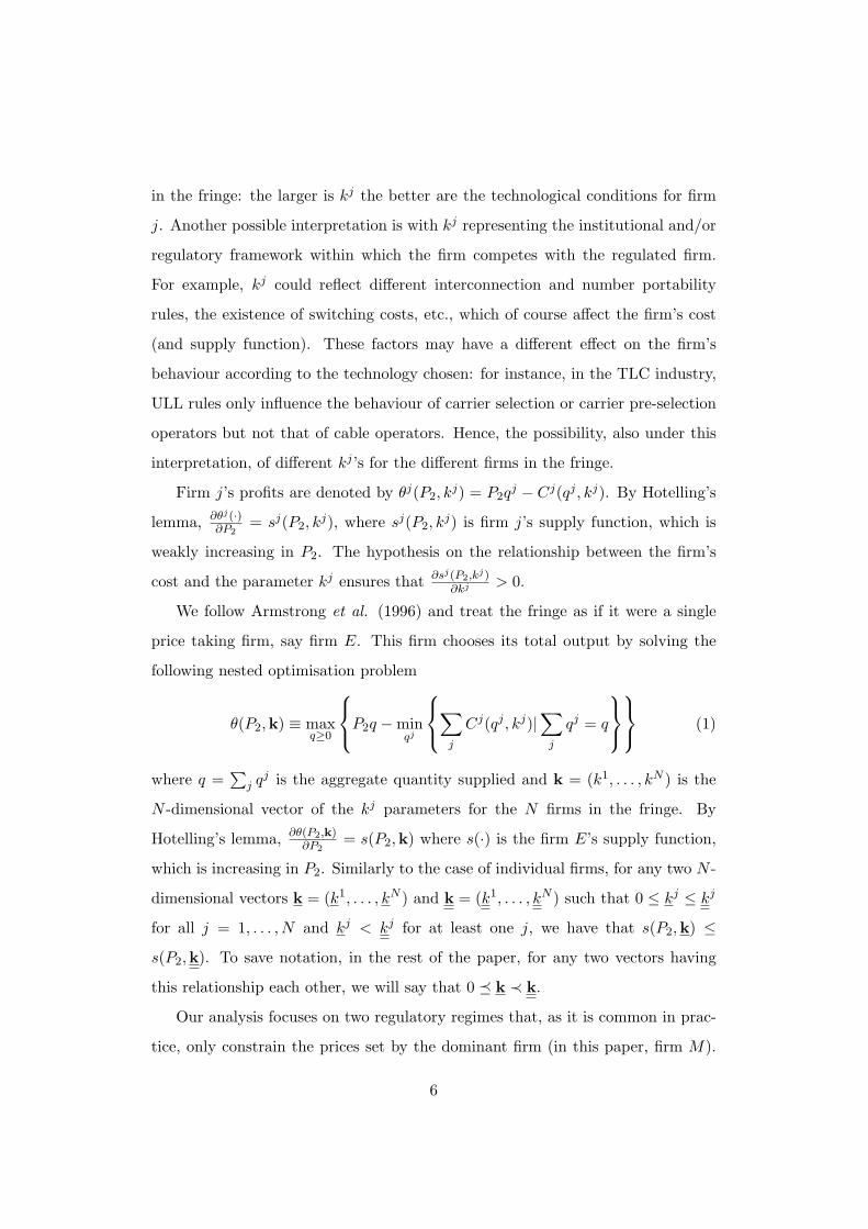
Similarly, under the Relative regime we find that

pR1 = 2k−c(k−1)

2(k+1) , pR2 = 2+c(k−1)

2(k+1) for 1 < k ≤ k′; (9)

pR1 = β

β+1 , pR2 = 1

β+1 for k′ ≤ k ≤ k′′′ (10)

pR1 = β(1+cβ+ck+β)

2(β2+k), pR

2 = 1+cβ+ck+β2(β2+k)

for k′′′ ≤ k ≤ kRmax; (11)

where k′ takes on the same value as before, k′′′ = β2(1−c)−β(2+c)−1βc−2+c and kR

max =1−β(1+c)+

√(1−cβ)2+β2(1+10c)−2β

2c . As in the case of the Absolute regime, k < kRmax

ensures that firm M faces a non–negative residual demand. Notice that kRmax <

kAmax for any admissible value of the parameters c and β.11

Notice that, when firm E offers either a null or a sufficiently small level of

output, optimal prices are identical to those set under the Absolute regime. On the

other hand, when k is sufficiently large, the price set by firm M in the competitive

market decreases with the supply level. Clearly, this is also what occurs under the11The additional conditions c ≤ 1

3ensures that k′′′ < kR

max. Although this condition is not

necessary for the analysis, it is assumed to hold for the sake of simplicity.

16

k kk kk

A

A

R

R2

1

2

1

p

pp

p

’’’ AR’’’maxmax

0.2

0.4

0.6

p

2 4

k

Figure 2: Equilibrium prices in the linear case (c = 0.2 and β = 1.1)

Absolute regime. However, under the Relative regime, because of the additional

constraint on the price ratio, if the regulated firm charges a low price in the

competitive market it is constrained to charge a low price in the captive market

as well. Hence, the larger the supply by firm E, the lower is the price in the

competitive market but also, differently than under the Absolute regime, the lower

is the price in the captive market.

In Figure 2 we plot against k the equilibrium prices under the two alternative

regimes, providing a graphical illustration of the results derived under more general

conditions in Propositions 1 and 2.

We now turn to analysing the welfare properties of the two regulatory rules.

The highly non linear nature of the welfare measures, evaluated at equilibrium

prices, prevents us from obtaining findings as general as in the previous sections.

Therefore, the analysis of the welfare properties of the two regimes is carried out by

means of numerical methods.12 We argue that this methodology does not unduly12Numerical computations and plots are made using the mathematical software Maple. Details

17

restrict the significance of our analysis. As a matter of fact, we aim at finding

plausible regularities in the conditions that ensure that one regime performs better

than the other in terms of guaranteeing higher social welfare. Numerical analysis

is, in our view, an appropriate, albeit maybe inelegant, instrument for this purpose.

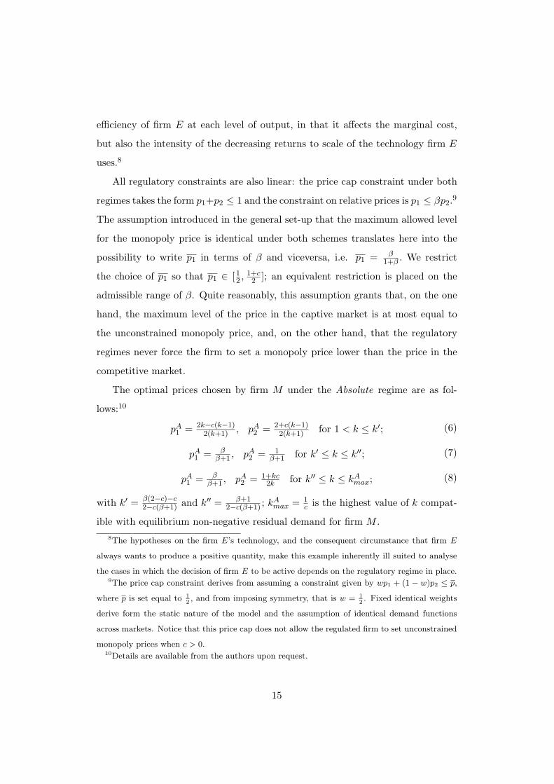
The difference between the equilibrium aggregate consumer surplus under the

Absolute regime and under the Relative regime is plotted in the top panel of Figure

3 against the technological variable k for different values of firm M ’s marginal cost

c and for a given value of β. The Figure shows that, when k is sufficiently low,

equilibrium prices do not differ across regimes and therefore aggregate consumers’

surplus is identical. When k is sufficiently large, the Absolute regime brings about

a higher consumer surplus. This is simply the effect of the Relative regime caus-

ing a higher competitive price, being the captive price identical across regimes.

Consumers may however prefer the Relative regime for high values of k when the

reduction in the monopoly price brought about by the Relative regime is able to

outplay the negative effects of the higher competitive price.

Also, for a given k, the advantages of the Relative regime are higher the lower

is the firm M ’s marginal cost. The reason for this is the following. As k increase,

firm E becomes more and more efficient and exerts more “competitive” downward

pressure on firm M ’s price for good x2. This competitive pressure is more costly

to firm M in the Relative regime, since the reduction of the competitive price must

be coupled, under this regime, with a reduction of the captive price. The more

inefficient is firm M , the more unwilling this firm will be to lower its price as a

reaction to an increase in the competitive pressure from the rival firm. Clearly, for

the reasons illustrated above, this reluctance increases under the Relative regime,

leading firm M to charge relatively higher prices under the Relative regime when

it has a high cost parameter.13

are available from the authors upon request.13Notice that, although we do not we allow for this possibility in our analysis, it may be the case

that the regulatory authority weights more the welfare of consumers in the captive market. In

our model, for any given technological conditions, this would enhance the benefits of the Relative

18

c=0.3

c=0.25

c=0.2

c=0.15

c=0.1

c=0.05–0.15

–0.1

–0.05

02 3 4 5

k

c=0.3

c=0.25

c=0.2

c=0.15

c=0.1

c=0.05

–0.02

0

0.02

0.04

0.06

0.08

2 3 4 5

k

c=0.3

c=0.25

c=0.2

c=0.05

c=0.15

c=0.1

–0.06

–0.04

–0.02

0

0.02

2 3 4 5k

Figure 3: Differences between the equilibrium aggregate consumer surplus (panel

1), aggregate profits (panel 2) and overall welfare (panel 3) under the Absolute

and the Relative regimes in the linear case (β = 1.1).

19

Likewise, we plot in the middle panel of Figure 3 the difference between the

equilibrium aggregate profits under the Absolute and the Relative regime against

the technological variable k for different values of firm M ’s marginal cost c and for

a given value of β. No difference between the regime is observed for very low val-

ues of k. When k takes an intermediate value, the Relative regime delivers higher

aggregate profits. This is because the higher competitive price under this regime

clearly makes both firms better off. When k is sufficiently large, the advantages in

terms of aggregate profits from the Absolute regime increase with k. Indeed, the

larger is k the more vigorously competition drives down the price in the competi-

tive market, increasing the quantity traded and its production cost, and thereby

reducing aggregate profits obtained in this market. Since we have already observed

that this effect is weaker under the Relative regime, this would seem to favour this

regime in terms of aggregate profits. Another reason for reaching this conclusion

would be related to cost considerations: under the Relative regime, firm E’s sup-

ply is larger and, given its decreasing return to scale, aggregate production cost in

this market are higher. However, under this same regime, when the competitive

price is reduced, also the captive price is forced down: it is then the joint effect

on the two markets that makes the Relative regime deliver lower aggregate profits

at high values of k. For exactly the same reason illustrated when discussing to

the relationship between consumers surplus and the firm M ’s marginal cost, this

negative effect of the Relative regime on aggregate profits is more likely to outplay

its positive effect when c is low.14

The bottom panel of Figure 3 illustrates the difference between the equilibrium

social welfare under the two regimes. It clearly emerges that the effect on consumer

regulatory regime. Clearly, this is because, under this regime, the captive price is always weakly

lower then under the alternative regulatory rule.14Similarly to footnote 13, it may be the case that the regulatory authority weights more the

profits obtained by the competitor than those of the regulated firm. As in the case of consumers’

surplus, this would clearly strengthen the argument in favour of the Relative regime, since prices

and, therefore, profits are always weakly higher in this market under this regime.

20

surplus dominates the effect on profits; afortiori, this would be even truer had we

assumed a social welfare function weighting consumers’ surplus more than profits.

5 Conclusions

This paper has analysed the effects of different approaches for limiting the pricing

discretion of a price capped firm which faces different degrees of competition in

the markets it serves. This issue is of a particular importance when the regulated

firm is price capped, since it has been shown in the literature that this firm can

exploit its freedom in setting prices to hinder the development of competition.

This issue is also relevant when a liberalisation process reaches its more advanced

stages, where price constraints in the relatively competitive markets are completely

abolished; in this case, the key question is whether or not the level of the remaining

price constraints should be somehow linked to the prices prevailing in the more

competitive markets.

The main policy implication that can be derived from this paper is that the use

of cross-market restrictions may be part of a regulatory policy promoting competi-

tion. This type of constraints are more likely to enhance consumers’ welfare (and

reduce aggregate firms’ profits) the higher is the degree of competition in the po-

tentially competitive markets. In our model, it is a better technology and/or more

favourable institutional arrangements that foster competition both in terms of a

greater supply and/or in terms of a larger number of firms entering the market.

We derived our results in a highly stylised setting. However, we believe that

a richer model could do nothing but strengthen them.15 In particular, a dynamic

model could take fully account of the dynamic advantages of a more competi-

tive market. Moreover, a model allowing for a strategic interaction between firms15Our results are also robust to different specifications of the model; in particular, we have

obtained results very similar to those illustrated here in a model where the entrant chooses its

capital while facing a convex cost of capital of installation, and then chooses the level of output

per unit of capital installed.

21

would lead to a higher competitive pressure on the regulated incumbent, thereby

enhancing the likelihood of cross-market price restrictions to make consumers bet-

ter off.

References

[1] Anton, J. J., J. H. Vander Weide and N. Vettas (2002). “Entry auctions and

strategic behaviour under cross-market price constraints”. International

Journal of Industrial Organization, 20, 611-629.

[2] Armstrong, M., S. Cowan and J. Vickers (1994). Regulatory Reform: Eco-

nomic Analysis and British Experience. Cambridge (MA): MIT Press.

[3] Armstrong, M., C. Doyle and J. Vickers (1996). “The Access Price Problem:

A Synthesis”. Journal of Industrial Economics, XLIV, 131-50.

[4] Armstrong, M. and D. E. M. Sappington (forthcoming). “Recent Develop-

ments in the Theory of Regulation”. In M. Armstrong and R. H. Porter

(eds.): Handbook of Industrial Organization: Volume 3. Amsterdam:

North-Holland.

[5] Armstrong, M. and J. Vickers (1991). “Welfare Effects of Price Discrimination

by a Regulated Monopolist”. RAND Journal of Economics, 22, 571-580.

[6] Armstrong, M. and J. Vickers (1993). “Price discrimination, competition and

regulation”. Journal of Industrial Economics, XLI, 335-59.

[7] Armstrong, M. and J. Vickers (2000), “Multiproduct Price Regulation under

Asymmetric Information”. Journal of Industrial Economics, XLVIII(4),

137-160.

[8] Bos, D. and L. Nett (1990). “Privatization, price regulation, and market

entry. An asymmetric multistage duopoly model”. Journal of Economics

- Zeitschrift fur Nationalokonomie, 51, 221-57.

[9] Iozzi A. (2001). “Strategic Pricing and Entry Deterrence under Price Cap

22

Regulation”. Journal of Economics - Zeitschrift fur Nationalokonomie,

74 (3), 283-301.

[10] Iozzi A. and M. Fioramanti (2004). “Strategic Choice of the Price Structure

and Entry Deterrence under Price Cap Regulation”. Bulletin of Economic

Research, 56 (4), 333-52.

[11] Ireland, N. J. (1992). “On the Welfare Effects of Regulating Price Discrimi-

nation”. Journal of Industrial Economics, XL(3), 237-248.

[12] Ofgem, 2003. Electricity Distribution Price Control Review – Metering Isuues:

Initial Consultation. Office of Gas and Electricity Markets, July.

[13] Otero, J. and C. Waddams Price (2001). “Price Discrimination, Regulation

and Entry in the UK Residential Electricity Market”. Bulletin of Eco-

nomic Research, 53:3, 161-175.

[14] Varian, H. (1989). “Price Discrimination”, in Schmalensee, R. and R. Willig

(eds.), Handbook of Industrial Organization. Amsterdam: North Holland.

[15] Vickers, J. (2004). “Abuse of market power”. Speech delivered to the 31st con-

ference of the European Association for Research in Industrial Economics,

Berlin.

[16] Vogelsang, I. and J. Finsinger (1979). “A regulatory adjustment for optimal

pricing by multiproduct monopoly firm”. Bell Journal of Economics, 10,

157-71.

23