Asset-pricing puzzles and price-impact∗ - American ...

Asset-pricing puzzles and price-impact∗

Xiao Chen

Rutgers University

Jin Hyuk Choi

Ulsan National Institute of Science and Technology (UNIST)

Kasper Larsen

Rutgers University

Duane J. Seppi

Carnegie Mellon University

November 13, 2020

Abstract: We solve in closed-form a continuous-time Nash equilibrium model

in which a finite number of exponential investors continuously consume and

trade strategically with price-impact. Compared to the analogous Pareto-

efficient equilibrium model, price-impact has an amplification effect on risk-

sharing distortions that helps resolve the interest rate puzzle and the stock-

price volatility puzzle. However, price impact has little effect on the equity

premium puzzle.

Keywords: Asset pricing, price-impact, Nash equilibrium, Radner equilibrium,

risk-free rate puzzle, equity premium puzzle, volatility puzzle.

∗The authors have benefited from helpful comments from Yashar Barardehi, Suleyman Basak, Rene Carmona,George Constantinides, Joel Hasbrouck, Burton Hollifield, Ioannis Karatzas, Lars Kuehn, Bryan Routledge,Mete Soner, Chris Telmer, and seminar participants at Tepper (Carnegie Mellon), ORFE (Princeton), andIntech. The third author has been supported by the National Science Foundation under Grant No. DMS1812679 (2018 - 2021). Any opinions, findings, and conclusions or recommendations expressed in this materialare those of the author(s) and do not necessarily reflect the views of the National Science Foundation (NSF).The corresponding author is Duane J. Seppi. Xiao Chen has email: [email protected], Jin Hyuk Choihas email: [email protected], Kasper Larsen has email: [email protected], and Duane J. Seppi hasemail: [email protected].

Electronic copy available at: https://ssrn.com/abstract=3465159

1 Introduction

Understanding the effects of market frictions on pricing and trading is a long-standing

topic of interest in financial economics. The market microstructure literature focuses on

informational and liquidity-provision frictions (e.g., Kyle 1985, Stoll 1978, Grossman and

Miller 1998). In contrast, the consumption-based asset pricing literature studies how vari-

ous frictions affect risk-sharing across investors and, thus, affect interest rates, stock-price

volatility, and the market price-of-risk.1 This paper merges these two approaches and inves-

tigates the asset-pricing effects of trading by strategic investors with price-impact frictions

on continuous-time stock-price dynamics and interest rates.

Much of our modeling approach is standard. A finite number of risk-averse investors

with time-separable utility receive individual income over time and trade a stock that pays

exogenous continuous dividends and a money market account. Consumption and trading

decisions occur in continuous time over a finite time horizon. Investors trade due to initial

stock-holding endowment imbalances. Following Vayanos (1999), investors are strategic

with respect to the perceived price-impact of their asset holdings and trades. Our main

theorem provides the continuous-time Nash equilibrium stock-price process and equilibrium

interest rate with price-impact via solutions to a system of ODEs.

Our main application shows that price-impact in our Nash equilibrium model has mate-

rial effects on the equilibrium interest rate and stock-price process relative to both the anal-

ogous competitive price-taking Radner equilibrium (with unspanned income shocks and no

1Previous research shows that model incompleteness and consequent non-efficient risk-sharing equilibriacan arise from several channels including: (i) Unspanned labor income as in the continuous-time Radnermodels in Christensen, Larsen, and Munk (2012), Zitkovic (2012), Christensen and Larsen (2014), Choi andLarsen (2015), Kardaras, Xing, and Zitkovic (2015), Larsen and Sae-Sue (2016), and Weston and Zitkovic(2020). (ii) Limited stock-market participation and trading constraints as in the continuous-time Radnermodels in Basak and Cuoco (1998), Chien, Cole, and Lustig (2011), and Hugonnier (2012). (iii) Transactioncosts and quadratic penalties as in the Radner models in Heaton and Lucas (1992, 1996), Vayanos andVila (1999), Garleanu and Pedersen (2016), Bouchard, Fukasawa, Herdegen, and Muhle-Karbe (2018), andWeston (2018). (iv) Trading targets as in the continuous-time Nash models in Brunnermeier and Petersen(2005), Sannikov and Skrzypacz (2016), and Choi, Larsen, and Seppi (2020). (v) Price-impact as in thediscrete-time Nash model in Vayanos (1999) and the continuous-time Nash models in Basak (1996, 1997).

1


price-impact) and the analogous Pareto-efficient equilibrium (with spanned income shocks

and no price-impact). More specifically, taking the Pareto-efficient equilibrium model as

a baseline, price-impact in our Nash equilibrium model magnifies risk-sharing distortions

and, as a result, simultaneously lowers the interest rate and increases stock-price volatil-

ity. Therefore, price-impact simultaneously helps resolve the risk-free rate puzzle of Weil

(1989) and the volatility puzzle of LeRoy and Porter (1981) and Shiller (1981). However,

price-impact has no impact on the instantaneous Sharpe ratio and has quantitatively little

effect on the finite-horizon Sharpe ratios for reasonable model parameters. Thus, while

price-impact does have asset pricing effects on the interest rate and stock volatility, it does

not help resolve the equity premium puzzle of Mehra and Prescott (1985). To the best of

our knowledge, our results about price-impact and asset-pricing puzzles are new.

A variety of other approaches have been proposed to resolve asset-pricing puzzles: (i)

Constantinides and Duffie (1996) and related work in Storesletten, Telmer, and Yaron (2007,

2008) and Krueger and Lustig (2010) use permanent idiosyncratic income shocks to resolve

the three asset-pricing puzzles. However, Cochrane (2005, p.478-9) argues that high levels

of risk aversion are still needed to explain the equity premium puzzle in Constantinides

and Duffie (1996). Cochrane (2008, p.310) argues that jumps help the continuous-time

limiting model of Constantinides and Duffie (1996) to explain the puzzles.2 Constantinides

(2008) and Constantinides and Gosh (2017) make related points about skewedness. In

contrast to approach (i), our price-impact equilibrium model has modest levels of risk

aversion and no jumps or skewedness. In particular, we use correlated arithmetic Brownian

motions to generate exogenous stock dividends and strategic investor idiosyncratic income

shocks.3 (ii) In a representative agent framework, Constantinides (1990) uses an internal

habit process and Campbell and Cochrane (1999) use an external habit process to explain

2Larsen and Sae-Sue (2016) give a closed-form competitive Radner equilibrium model with exponentialutility investors and dividend and income processes governed by continuous-time Levy jump processes thatcan simultaneously explain the three puzzles.

3Additionally, Judd (1985), Feldman and Gilles (1985), and Uhlig (1996) present both mathematical andinterpretation issues related to models with a continuum of investors — such as Constantinides and Duffie(1996) — because these models rely on average clearing conditions. In contrast, our equilibrium model’sidiosyncratic income shocks do not average out at the aggregate level.

2


the puzzles. (iii) Bansal and Yaron (2004) combine long-run consumption risk and an

Epstein-Zin representative agent to explain the puzzles. (iv) Barro (2006) and the extension

to an Epstein-Zin representative agent in Wachter (2013) use rare disasters based on jump

processes to resolve the puzzles. In contrast to approaches (ii)-(iv), our investors’ utilities

are time-additive separable exponential utility functions over continuous-time consumption

rate processes. Furthermore, the models in approaches (ii)-(iv) are based on representative-

agent frameworks in which the underlying model is effectively complete. However, our model

incorporates unspanned income shocks and trading with price-impact. Of the models in (ii)-

(iv), our model is closest to the external habit model in Campbell and Cochrane (1999).

Indeed, by switching off our model’s idiosyncratic income shocks, the resulting common

income shocks can be interpreted as an external habit.

A non-standard feature is that our analysis is non-stationary in that the asset pricing

effects of price-impact dissipate over time. In our model, investors start with endowed ini-

tial stock positions that are Pareto inefficient. However, due to price-impact, investors do

not trade immediately to efficient risk-sharing; rather they trade gradually to optimize with

respect to a trade-off between the benefits of improved risk-sharing and price-impact costs

of faster trading. Over time, their gradual trading has a cumulative effect that improves

risk-sharing. Thus, our analysis shows that price-impact can have a quantitatively material

short-term amplification effect on asset pricing by prolonging risk-sharing distortions. In

our model, risk-sharing distortions arise as a one-time occurrence via inequalities in ini-

tial endowed stock positions. In richer economic settings, however, risk-sharing distortions

could arise on a reoccurring basis from shocks to stochastic habits, sentiment, income, het-

erogeneous beliefs, and asymmetric information. In such a reoccurring-shock environment,

the asset pricing amplification effect due to price-impact could be part of asset pricing in a

stationary equilibrium. Moreover, from a calibration perspective, fundamental risk-bearing

shocks can be quantitatively smaller (i.e., more realistic) and still have material asset pricing

effects because they would be magnified by the price-impact amplification effect.

Basak (1996, 1997), Vayanos (1999, 2001), and Pritsker (2009) are earlier equilibrium

3


models of strategic trading with price-impact. The main differences between our model and

Basak (1996, 1997) are: First, unspanned income shocks make our model incomplete. Sec-

ond, we allow for multiple traders with price-impact. Third, our price-impact equilibrium

model is time-consistent. Our analysis extends or differs from seminal work by Vayanos

(1999, 2001) and from Pritsker (2009) in three ways: First, we focus directly on puzzles

in asset pricing moments, whereas Vayanos (1999) studies welfare but not asset pricing

moments. Second, we solve for an endogenous deterministic interest rate. This allows us

to investigate the interest rate puzzle in Weil (1989). Importantly, it also allows us to

derive the effect of price-impact on the equity premium taking into account the effect of

price-impact on endogenous interest rates. In particular, we find that price-impact has a

quantitatively larger effect on endogenous interest rates than on the equity Sharpe ratio.

Third, our investors start with non-Pareto efficient initial stock endowments but then subse-

quently receive stochastic personal income shocks. This seems more realistic than dynamic

stock-holding shocks as in Vayanos (1999).4 Fourth, and more technically, our model is in

continuous time, which makes the analysis mathematically tractable. Our main theoretical

result ensures existence of a solution to a coupled forward-backward system of ODEs. This

solution is subsequently used to give existence of a Nash equilibrium, which we solve in

closed-form.

Our analysis is related to a long-standing question in financial economics about whether

liquidity is priced (see, e.g., surveys in Easley and O’Hara (2003) and Amihud, Mendel-

son, and Pedersen (2006)). One literature holds that liquidity is priced because investors

require compensation for holding securities that expose them to higher transaction costs.

For example, Amihud and Mendelson (1986) provide a theoretical analysis of this cost-

compensation effect. Acharya and Pedersen (2005) also show that systematic uncertainty

in stochastic trading costs (seen as a type of random negative dividends) can be a priced risk

factor. However, another literature argues that the quantitative impact of liquidity on asset

pricing is small by showing in various economic settings that investors can, given trading

4Vayanos (2001) allows for exogenous noise traders, but all our investors are utility maximizers.

4


costs, reduce their trading with only small utility costs. This counter-argument was first

presented in Constantinides (1986). In contrast, our model is not about bid-ask spreads

and transactional forms of illiquidity, but rather about the price-impact of investor asset-

demand imbalances on market-clearing prices. In particular, we show, in an analytically

tractable version of a standard general equilibrium asset pricing framework, how gradually

decaying distortions in risk-sharing due to how investors curtail their trading in response

to price-impact has asset-pricing effects. We find that price-impact affects prices through

interest rate and return volatility channels but not via the market price-of-risk. Thus, our

analysis supports the equity-premium argument in Constantinides (1986).

2 Setup

We consider a real economy model with a single perishable consumption good, which we take

as the model’s numeraire. Trading and consumption take place continuously for t ∈ [0, T ]

for a finite time-horizon T ∈ (0,∞). The model has two traded securities: A money market

account and a stock. The money market account is in zero net supply, and the stock supply

is a constant L ∈ N. The stock pays exogenous random dividends given by a rate process

D = (Dt)t∈[0,T ] per share. We model the asset-holding and consumption decisions of a

group of i ∈ {1, ..., I}, I ∈ N, strategic traders. Investors receive individual income given

by exogenous random rate processes Yi = (Yi,t)t∈[0,T ] for i ∈ {1, ..., I}. In Theorem 3.3

below, we determine endogenously the interest rate r =(r(t)

)t∈[0,T ]

(a deterministic time-

varying function) and the stock-price process S = (St)t∈[0,T ] in a Nash equilibrium with

price-impact.

2.1 Exogenous model inputs

Let (Bt,W1,t, ...,WI,t)t∈[0,T ] be a set of independent one-dimensional Brownian motions

starting at zero with zero drifts and unit volatilities. The augmented standard Brownian

5


filtration is denoted by

Ft := σ(Bs,W1,s, ...,WI,s)s∈[0,t], t ∈ [0, T ]. (2.1)

An exogenous stock dividend rate process Dt has dynamics

dDt := µDdt+ σDdBt, D0 ∈ R, (2.2)

driven by the Brownian motion Bt, with a given initial value D0, a constant drift µD, and

a constant volatility coefficient σD ≥ 0.5 The dividend rate process plays two roles: First,

it generates a running flow of instantaneous dividends where the associated cumulative

dividend over [0, t] is∫ t

0 Dsds for t ∈ [0, T ]. Second, the stock pays a terminal discrete

liquidating dividend DT at the terminal date T that pins down the terminal stock price:

limt↑T

St = DT , P-a.s. (2.3)

The terminal condition (2.3) requires the stock-price process S = (St)t∈[0,T ] to be left-

continuous at time t = T . We refer to Ohasi (1991, 1992) for a discussion of (2.3). A

boundary condition like (2.3) is needed since our model, for mathematical tractability, has

a finite time horizon. However, by making T large, the terminal liquidating dividend DT is

small relative to total dividends∫ T

0 Dsds + DT . In the next section, we require that (2.3)

holds for each investor i’s perceived stock-price process S = Si (to be defined in Section 2.3)

and for the equilibrium stock-price process S = S (to be derived in Section 3). Models with

terminal Gaussian dividends include Grossman and Stiglitz (1980) and Kyle (1985), and

models with running Gaussian dividends include Campbell, Grossman, and Wang (1993),

Vayanos (1999), and Christensen, Larsen, and Munk (2012).

We model the income rate process Yi,t for trader i ∈ {1, ..., I} as in Christensen, Larsen,

5The assumption of Brownian motion dividends is for mathematical tractability. However, the initialdividend D0 and the dividend drift and volatility can be set such that the probability of negative dividendsis arbitrary small.

6


and Munk (2012) and define

dYi,t := µY dt+ σY(ρdBt +

√1− ρ2dWi,t

), Yi,0 ∈ R, (2.4)

where the Brownian motion Wi,t generates idiosyncratic income shocks. Investor i’s income

consists of a flow of income over [0, T ] resulting in cumulative income given by∫ T

0 Yi,sds

and then a lump-sum income payment Yi,T at the end. The terminal payment Yi,T is a

reduced-form for the value of a flow of income after the terminal date T . Similar to the

boundary condition for dividends, the terminal lump-sum income YT can be made small

relative to total income∫ T

0 Ysds+YT by making T large. In the income rate dynamics (2.4),

the given initial value is Yi,0, the constant drift is µY , the constant volatility coefficient is

σY ≥ 0, and ρ ∈ [−1, 1] is a correlation parameter controlling the relative magnitudes of

investor-specific (i.e., idiosyncratic) income shocks and systematic income shocks correlated

with the dividend process in (2.2). For example, ρ := 0 makes all individual income shocks

independent of dividend shocks. When ρ2 < 1 in (2.4), no single stock-price process can span

all risk because any model with multiple Brownian motions and only one stock is necessarily

incomplete by the Second Fundamental Theorem of Asset Pricing. However, when ρ2 = 1,

all randomness in the model is due to the Brownian motion Bt, and model completeness is

possible. The assumption of homogenous income coefficients across investors is common in

many Nash equilibrium models.

The strategic traders’ endowed money market balances are normalized to zero. Traders

begin with exogenous initial individual stock endowments equal to constants θi,0 ∈ R for

i ∈ {1, ..., I}. Their stock-holding processes over time are

θi,t := θi,0 +

∫ t

0θ′i,udu, t ∈ [0, T ]. (2.5)

This restriction forces traders to use only holding processes given by continuous order-rate

processes θ′i,t. This rate-process restriction has been used in various equilibrium models

including Back, Cao, and Willard (2000), Brunnermeier and Pedersen (2005), Garleanu and

7


Pedersen (2016), and Bouchard, Fukasawa, Herdegen, and Muhle-Karbe (2018). Section 5

below shows how to incorporate discrete orders (i.e., block trades) into the model.

At each time t ∈ [0, T ], trader i chooses an order-rate θ′i,t and a consumption rate ci,t.

In aggregate, trading and consumption clear the stock and real-good consumption markets

in the sense that

L =I∑i=1

θi,t, LDt +I∑i=1

Yi,t =I∑i=1

ci,t, t ∈ [0, T ], (2.6)

where L is the constant stock supply. Walras’ law ensures that clearing in the stock and

real-good consumption markets lead to clearing in the zero-supply money market. The

terminal stock price (2.3) ensures clearing in the real good consumption market at the

terminal time T .

Our model is constructed to investigate how price-impact affects risk-sharing and, thus,

asset pricing. Two specific risk-sharing distortions are present in the model: The first is

potential deviations of investors’ initial endowments θi,0 from equal holdings LI . A second

potential distortion is unspanned stochastic investor income. Section 3 investigates both

distortions.

2.2 Individual utility-maximization problems

With price-impact in our model, traders perceive that their holdings θi,t and order rates

θ′i,t affect the prices at which they trade and their resulting wealth dynamics. In particular,

price-impact here is due to a persistent impact of investor holdings on the market-clearing

aggregate risk-bearing capacity of the market and due to a transitory microstructure impact

of investor trading. Trader i’s perceived wealth process is defined by

Xi,t := θi,tSi,t +Mi,t, t ∈ [0, T ], i ∈ {1, ..., I}, (2.7)

where θi,t denotes her stock holdings, Si,t is her perceived stock-price process, and Mi,t is

her money-market balance (all these processes are to be determined in equilibrium endoge-

8


nously). In a Nash equilibrium model, the perceived stock-price processes Si,t in (2.7) can

differ off-equilibrium across different traders i given their different hypothetical holdings θi,t

and trades θ′i,t but the equilibrium stock-price process St is identical for all traders. On the

other hand, we assume all traders perceive the same deterministically time-varying interest

rate r(t), t ∈ [0, T ] (to be determined endogenously).

Recall that each strategic trader’s initial money market account balance is normalized

to zero, whereas the initial endowed stock holdings are exogenously given by θi,0 ∈ R. The

self-financing condition produces trader i’s perceived wealth dynamics

dXi,t = r(t)Mi,tdt+ θi,t(dSi,t +Dtdt) + (Yi,t − ci,t)dt, Xi,0 = θi,0Si,0. (2.8)

As usual in continuous-time stochastic control problems, the traders’ controls must

satisfy various regularity conditions.

Definition 2.1 (Admissibility). An order-rate process θ′i = (θ′i,t)t∈[0,T ] and a consumption-

rate process ci = (ci,t)t∈[0,T ] are admissible, and we write (θ′i, ci) ∈ A if:

(i) The processes (θ′i, ci) have continuous paths and are progressively measurable with

respect to the filtration Ft in (2.1).

(ii) The stock-holding process θi,t defined by (2.5) is uniformly bounded.

(iii) The wealth process dynamics (2.8) as well as the corresponding money market account

balance process Mi,t := Xi,t − Si,tθi,t are well-defined and

supt∈[0,T ]

E[eζMi,t ] <∞ for all constants ζ ∈ R. (2.9)

(iv) The perceived stock-price process Si,t satisfies the terminal condition (2.3).

♦

9


Each trader i seeks to solve6

inf(θ′i,ci)∈A

E[∫ T

0e−aci,t−δtdt+ e−a(Xi,T+Yi,T )−δT

], i = 1, ..., I, (2.10)

given the perceived stock-price process Si,t in her wealth dynamics (2.8). In (2.10), the term∫ T0 e−aci,t−δtdt denotes utility from the consumption flow rates, and the term e−a(Xi,T+Yi,T )−δT

is a bequest value function for terminal wealth. Like the terminal dividend DT and the

lump-sum terminal income YT , the bequest utility function proxies for continuation utility

past the terminal time in our model. For tractability, the common absolute risk-aversion

coefficient a > 0 is the same for both the consumption flow utility and the bequest value

function. The common time preference parameter is δ ≥ 0. The assumption of identical

exponential utilities across investors is common in many Nash equilibrium models, see, e.g.,

Vayanos (1999).

The next subsection derives stock-price dynamics perceived by trader i when solving

(2.10) as part of our Nash equilibrium with price-impact. These perceived price dynamics

differ from those in the competitive Radner and Pareto-efficient equilibria where all traders

perceive the same stock price and act as price-takers. We describe the analogous competitive

Radner equilibrium in Appendix C and the analogous competitive Pareto-efficient equilib-

rium in Appendix D. As is shown below, neither our Nash model with price-impact nor

the analogous competitive Radner model is Pareto efficient. In addition, when the idiosyn-

cratic income shocks are turned off, the Radner equilibrium reduces to the Pareto-efficient

equilibrium, whereas our Nash model remains Pareto inefficient due to price-impact.

2.3 Price-impact for the stock market

The perceived stock-price process Si,t for trader i depends on market-clearing given how

the other traders j ∈ {1, ..., I} \ {i} respond to trader i’s hypothetical choices of θ′i,t. Thus,

for a Nash equilibrium, we must model how traders j, j 6= i, respond to an arbitrary control

6The negative sign in the exponential utility is removed for simplicity, which leads to the minimizationproblem in (2.10).

10


θ′i,t used by trader i.

Several different price-impact models are available in the literature: Kyle (1985) and

Back (1992) use continuous-time price-impact functions in which price changes dSi,t are

affine in orders dθi,t. Cvitanic and Cuoco (1998) take the drift process in dSi,t to be a

function of θi,t. The affine price-impact function (2.14) we derive below can be found in the

single-trader optimal order-execution models in Almgren (2003) and Schied and Schoneborn

(2009). Our Nash equilibrium model with price-impact can be seen as a continuous-time

version of the discrete-time Nash equilibrium model in Vayanos (1999) in which Si,tn is

affine in discrete orders ∆θi,tn .

We conjecture that each generic trader i ∈ {1, ..., I} perceives the responses used by the

other traders j, j 6= i, to hypothetical holdings θi,t and trades θ′i,t by investor i as given by

θ′j,t := A0(t)(F (t)Dt − Si,t

)+A1(t)θj,t +A2(t)θi,t +A3(t)θ′i,t, j 6= i, (2.11)

for deterministic functions of time A0(t), ..., A3(t). The intuition behind (2.11) is that

investors j 6= i are perceived by investor i to have base levels for their orders θ′j,t that they

then adjust given the controlled price level Si,t (which is affected by trader i’s holdings θi,t

and orders θ′i,t) relative to an adjusted dividend level F (t)Dt where F (t) is the annuity7

F (t) :=

∫ T

te−∫ st r(u)duds+ e−

∫ Tt r(u)du, t ∈ [0, T ]. (2.12)

The response specification in (2.11) also allows the perceived responses of investors j 6= i to

depend directly on investor i’s hypothetical holdings θi,t and orders θ′i,t. Thus, Si,t is not

assumed to be a sufficient statistic for the effects of θi,t and θ′i,t on θ′j,t. At the end of this

subsection, we show that (2.11) can be rewritten as trader j deviating from j’s equilibrium

behavior in response to trader i’s off-equilibrium behavior. The model is symmetric in that

each trader i ∈ {1, ..., I} has perceptions of the form in (2.11).

The perceived investor-response functions A0(t), ..., A3(t) in (2.11) are not simply as-

7For future reference, note that (2.12) is equivalent to F (T ) = 1 and F ′(t) = r(t)F (t) − 1.

11


sumed. Rather, these functions are endogenously determined in equilibrium in Theorem 3.3

below given market-clearing, certain belief-consistency conditions (described in Definition

3.1 below), and given a microstructure parameter that implicitly determines the temporary

(transitory) price-impact of trading θ′i,t (see Theorem 3.3 below).

Investor i does not care directly about other investors’ trades and holdings per se, but

she does care about the impact other investor’s responses to i’s trades and holdings have on

the market-clearing prices at which trader i trades. In particular, the stock-price process

Si,t trader i perceives in her optimization problem (2.10) is found using the stock-market

clearing conditions (2.6) given the perceived responses in (2.11):

0 = θ′i,t +∑j 6=i

θ′j,t

= θ′i,t + (I − 1)A0(t)(F (t)Dt − Si,t

)+A1(t)(L− θi,t) + (I − 1)

(A2(t)θi,t +A3(t)θ′i,t

).

(2.13)

Provided that A0(t) 6= 0 for all t ∈ [0, T ], we can solve (2.13) for trader i’s perceived

market-clearing stock-price process:

Si,t = DtF (t) + A1(t)LA0(t)(I−1) + A2(t)(I−1)−A1(t)

A0(t)(I−1) θi,t + A3(t)(I−1)+1A0(t)(I−1) θ′i,t. (2.14)

Trader i’s stock holdings θi,t and orders θ′i,t affect the perceived stock-price process (2.14)

as follows. Similar to Almgren (2003), the sum F (t)Dt + A1(t)LA0(t)(I−1) in (2.14) is called the

fundamental stock-price process. The coefficient A2(t)(I−1)−A1(t)A0(t)(I−1) on holdings θi,t in (2.14)

is the permanent price-impact (positive in equilibrium) because the price-impact effect of

investor i’s past trading persists even after trading stops (when θ′i,t = 0 and θi,t 6= 0). The

coefficient A3(t)(I−1)+1A0(t)(I−1) on the order rate θ′i,t in (2.14) is the temporary price-impact (positive

in equilibrium) because this component of the price-impact effect disappears when investor i

stops trading (i.e., when θ′i,t = 0). Theorem 3.3 below provides A0(t), ..., A3(t) via solutions

to a system of coupled ODEs.

12


To see that (2.10) is a quadratic minimization problem given the perceived stock-price

process (2.14), we use the perceived money-market account balance process Mi,t from (2.7)

defined by

Mi,t := Xi,t − θi,tSi,t, i ∈ {1, ..., I}, (2.15)

as a state-process. The wealth dynamics (2.8) produce the following perceived dynamics of

the money-market account balance process

dMi,t = dXi,t − d(θi,tSi,t)

= r(t)Mi,tdt+ θi,t(dSi,t +Dtdt) + (Yi,t − ci,t)dt− θ′i,tSi,tdt− θi,tdSi,t

=(r(t)Mi,t + θi,tDt − Si,tθ′i,t + Yi,t − ci,t

)dt.

(2.16)

The second equality in (2.16) uses the quadratic variation property 〈θi, Si〉t = 0, which holds

because θi,t satisfies the order-rate condition (2.5). As shown in the proof in Appendix B,

the affinity in the price-impact function (2.14) and the last line in (2.16) make the individual

optimization problems (2.10) tractable.

Trader i’s control θ′i,t appears in trader j’s response (2.11) implicitly through the stock-

price process Si = (Si,t)t∈[0,T ] and directly via θi,t and θ′i,t. Substituting (2.14) for Si,t into

(2.11), the resulting response functions for j 6= i give trader j’s response directly in terms

of trader i’s orders θ′i,t and associated holdings θi,t, where trader j’s response is affine in

those quantities:

θ′j,t = A1(t)θj,t +A1(t)

1− I(L− θi,t) +

1

1− Iθ′i,t. (2.17)

Furthermore, the equilibrium holdings (θi,t, θj,t) and order-rate processes (θ′i,t, θ′j,t) in The-

orem 3.3 below are consistent with (2.11) in the sense

θ′j,t = A0(t)(F (t)Dt − St

)+A1(t)θj,t +A2(t)θi,t +A3(t)θ′i,t, j 6= i, (2.18)

13


given the equilibrium stock-price process St. This allows us re-write (2.17) as

θ′j,t = θ′j,t −A1(t)(θj,t − θj,t) +1

I − 1(θ′i,t − θ′i,t)−

A1(t)

I − 1(θi,t − θi,t). (2.19)

Thus, the responses in (2.19) describe deviations of θ′j,t from equilibrium behavior θ′j,t for

trader j, j 6= i, in response to trader i’s off-equilibrium deviations of θ′i,t from θ′i,t. Note

here that the equilibrium holdings (θi,t, θj,t) and order-rate processes (θ′i,t, θ′j,t), j 6= i, in

(2.19) do not depend on trader i’s arbitrary orders θ′i,t and holdings θi,t.

2.4 Modeling approach

This section briefly describes modeling differences between our analysis and other asset

pricing models and explains the motivation and reasons for these differences. Our analysis

is at the intersection of research on continuous-time asset pricing and dynamic trading by

heterogenous investors. Thus, for tractability, our model combines modeling elements from

both types of models. Our main technical contribution gives the existence of a tractable

continuous-time incomplete-market price-impact equilibrium. There are two key ingredients

in its construction: Price-impact perceptions as in Almgren (2003) and exponential utilities.

First, perceived price-impact, necessitates, for tractability, that we restrict investors to use

trading-rate processes, which, although less common than other continuous-time processes,

have been used in other equilibrium trading models including Back, Cao, and Willard (2000),

Brunnermeier and Pedersen (2005), and Garleanu and Pedersen (2016). Second, while not

as common as power and Epstein-Zin utilities, exponential utilities are used in asset pricing

equilibrium models in Calvet (2001), Wang (2003), Christensen, Larsen, and Munk (2012),

and Christensen and Larsen (2014). On the other hand, exponential utilities are standard

in the rational expectations trading literature as in, e.g., Grossman and Stiglitz (1980),

Campbell, Grossman, and Wang (1993), and Vayanos (1999). Since our model requires

trading and market-clearing by heterogenous investors (due to their heterogenous stock

holdings), exponential utilities make market-clearing tractable.

14


Endowment effects: With pricing-taking exponential investors, the initial endowed stock-

holding distribution across investors is irrelevant for asset-pricing models. This is well-

known and is re-derived in Appendices C and D. However, our exponential investors are

strategic in that they perceive their holdings and trades to have price-impact, which explains

why our equilibrium model exhibits stock-endowment effects. However, these endowment

effects are due to a risk-bearing mechanism rather than a wealth effect. When investors

are endowed with non-Pareto efficient initial stock endowments in terms of risk-sharing, it

is suboptimal for investors to trade immediately to their Radner allocations due to their

perceived costs given their perceived price-impact.8 The deviation of risk-sharing in the

model relative to the Radner equilibrium, in turn, affects investor stock demands, which

has price effects. It is this risk-sharing based endowment mechanism in our model that

affects risk-free interest rates and stock-price dynamics as mentioned in the introduction

and detailed in Section 4 below. The intuition behind the risk-sharing based endowment

mechanism is simple: It is costly to rebalance to efficient positions given price-impact.

Timing: Our model’s time horizon is finite but can be arbitrary long. Because of slow

trading due to price-impact, our investors’ heterogenous stock holdings converge gradually

over time to the Radner allocations over the time horizon. Consequently, our model is

non-stationary, and, in particular, the asset pricing effects of price-impact are short-term

in nature. However, to the extent that investors are repeatedly shocked away from efficient

risk sharing and need to trade, the model and its asset pricing effects could be made sta-

tionary. These could be periodic shocks to preferred holdings — due to fund flows causing

fluctuations in institutional assets under management (e.g., Coval and Stafford (2017)) and

changes in sentiment (e.g., Baker and Wurgler (2006)) — as well as to shocks to actual

holdings as in Vayanos (1999).

Illiquidity: Liquidity in general equilibrium asset pricing can be modeled as price-impact

or as transaction costs. Our price-impact approach follows Vayanos (1999) in modeling

liquidity as price pressure. Alternatively, transaction costs can be explicitly modeled search

8The Radner equilibrium is not Pareto efficient when ρ2 < 1 in (2.4). However, when ρ2 = 1, theidiosyncratic income shocks disappear and the Radner equilibrium becomes Pareto efficient.

15


costs (as in, e.g., Duffie, Garleanu, and Pedersen (2005)) or implicitly represented via a

reduced-form quadratic penalty (e.g., as in Garleanu and Pedersen (2016)), or can be fees

paid to intermediaries (i.e., bid-ask spreads and commissions charged by market makers,

brokers, and exchanges). Price-impact and transaction costs often produce similar implica-

tions for optimal investor consumption and portfolio choice, but there are other differences:

One difference is market clearing. Price pressure in prices is paid and received by all buyers

and sellers such that, by definition, markets clear. In contrast, transaction costs must either

be modeled as dissipative deadweight costs (i.e., costs for some investors but not income

for other market participants) or else market-making intermediaries must be modeled as

additional agents in the general equilibrium. A second difference concerns trading dynam-

ics. Bid-ask spread type transaction costs and commissions drive a wedge between the net

prices received by sellers and paid by buyers. Thus, as in Noh and Weston (2020), such

transaction costs can lead to endogenous possible no-trade. In contrast, there is no such

wedge with price-impact, and so there is no endogenous no-trade in our model. Third, price

pressure effects can be large if fundamental asset-holding imbalances are large. In contrast,

bid-ask spreads are compensation for short-term inventory holding. Thus, the ultimate as-

set buyers and sellers can keep these fees from being too large, absent adverse selection and

learning, by using dynamic trading to limit how much inventory intermediaries need to hold

at any point in time. Fourth, the quadratic penalty literature takes both permanent and

transitory transaction costs as exogenous. In contrast, Section 3 shows that persistent price

impact costs in our model, as in Vayanos (1999), are endogenously determined once the

transitory price impact is determined. Fifth, household trading constraints and exogenous

market participation restrictions (which can be viewed as infinite costs for certain types

of transactions) also affect asset pricing by distorting asset holdings (see footnote 1 for

references). In contrast, asset-holding distortions in our model are endogenous given that

price-impact slows investor adjustments responding to suboptimal risk-sharing.

16


3 Price-impact equilibrium

This section first defines a Nash equilibrium with price impact and then solves for the

equilibrium in closed-form.

3.1 Equilibrium definition

The following definition is a continuous-time version of the Nash equilibrium in Vayanos

(1999):

Definition 3.1 (Nash equilibrium). Perceived investor response coefficients given by contin-

uous functions of time A0, ..., A3 : [0, T ]→ R constitute a financial-market Nash equilibrium

if:

(i) The solution (ci,t, θ′i,t) to trader i’s individual optimization problem (2.10) with the

price-impact function (2.14) exists for all i ∈ {1, ..., I}.

(ii) The stock-price processes resulting from inserting trader i’s optimizer θ′i,t into the

price-impact function Si,t in (2.14) are identical for all traders i ∈ {1, ..., I}. This

common stock-price process, denoted by St, satisfies the terminal dividend restriction

(2.3).

(iii) The individual orders (θ′i,t)Ii=1 and corresponding holding processes (θi,t)

Ii=1 satisfy

the consistency requirement (2.18).

(iv) The real-good consumption market clearing and the stock-market clearing conditions

(2.6) hold at all times t ∈ [0, T ].

♦

A financial-market Nash equilibrium combines both the idea of strategic behavior in a

Nash equilibrium and the idea of market-clearing. In models of strategic trading, such as

Kyle (1985), this is often achieved by a liquidity provider who supplies residual liquidity

to clear the market. In contrast, following Vayanos (1999), our model constructs perceived

17


response functions in (2.11) for other strategic investors j 6= i such that markets clear given

any potential off-equilibrium trade θ′i,t by any generic investor i. In particular, this con-

struction leads to equation (2.19), which shows how other investors j 6= i deviate from their

equilibrium strategies θ′j,t in order for markets to clear in response to off-equilibrium trading

deviations θ′i,t of a generic investor i from her equilibrium strategy θ′i,t. Equilibrium strate-

gies are, therefore, fixed-points in that they are optimal responses to the perceived collective

off-equilibrium response functions of the other traders given the equilibrium strategies.9 We

also note here that our notion of equilibrium is defined in terms of the perceived price-impact

coefficients A0, ..., A3. These coefficients are the underlying primitives in our model. Given

the equilibrium price impact coefficients, we then solve for optimal strategies (ci,t, θi,t),

i ∈ {1, ..., I}, for investors given their equilibrium price perceptions as in a standard Nash

equilibrium.

3.2 Results

Our main existence equilibrium existence result is based on the following technical lemma

(the proof is in Appendix B below). It guarantees the existence of a solution to an au-

tonomous forward-backward system of coupled ODEs with forward component ψ and back-

ward components (F,Q2, Q22, Q). Similar forward-backward systems have appeared in equi-

librium theory. For example, in Kyle (1985), the forward component is the filter and the

backward components are the value-function coefficients.

Lemma 3.2. For all α > 0, there exists a constant w ≥ L2

I such that the unique solutions

9There are two further technical details to note here: First, for a Nash equilibrium we only need toconsider unilateral deviations from equilibrium strategies by individual investors rather than multilateraldeviations. Second, there is no infinite regress problem in our model (see Townsend (1983)). In a Nashequilibrium, strategies only need to be optimal with respect to perceptions of other agents’ behavior, butNash equilibrium does not require off-equilibrium beliefs to support that perceived behavior.

18


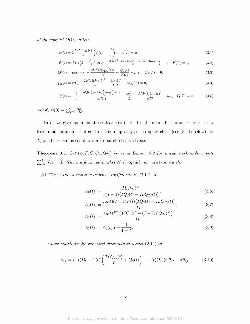
of the coupled ODE system

ψ′(t) = 2F (t)Q22(t)

α

(ψ(t) − L2

I

), ψ(T ) = w, (3.1)

F ′(t) = F (t)(δ − a2σ2

D2I

ψ(t) − a(aIσ2Y +2aLρσDσY −2IµY −2LµD)

2I

)− 1, F (T ) = 1, (3.2)

Q′2(t) = aρσDσY +2LF (t)Q22(t)2

αI+Q2(t)

F (t)− µD, Q2(T ) = 0, (3.3)

Q′22(t) = aσ2D − 2F (t)Q22(t)2

α+Q22(t)

F (t), Q22(T ) = 0, (3.4)

Q′(t) = − δa

+aQ(t) − log

(1

F (t)

)+ 1

aF (t)+aσ2

Y

2− L2F (t)Q22(t)2

αI2− µY , Q(T ) = 0, (3.5)

satisfy ψ(0) =∑I

i=1 θ2i,0.

Next, we give our main theoretical result. In this theorem, the parameter α > 0 is a

free input parameter that controls the temporary price-impact effect (see (3.10) below). In

Appendix E, we use calibrate α to match observed data.

Theorem 3.3. Let (ψ, F,Q,Q2, Q22) be as in Lemma 3.2 for initial stock endowments∑Ii=1 θi,0 = L. Then, a financial-market Nash equilibrium exists in which:

(i) The perceived investor response coefficients in (2.11) are

A0(t) :=ILQ22(t)

α(I − 1)(IQ2(t) + 2LQ22(t)

) , (3.6)

A1(t) :=A0(t)(I − 1)F (t)

(IQ2(t) + 2LQ22(t)

)IL

, (3.7)

A2(t) :=A0(t)F (t)

(IQ2(t)− (I − 2)LQ22(t)

)IL

, (3.8)

A3(t) := A0(t)α+1

1− I, (3.9)

which simplifies the perceived price-impact model (2.14) to

Si,t = F (t)Dt + F (t)

(2LQ22(t)

I+Q2(t)

)− F (t)Q22(t)θi,t + αθ′i,t. (3.10)

19


(ii) The equilibrium interest rate r(t) is given by

r(t) = δ −a2σ2

D

2Iψ(t)−

a(aIσ2

Y + 2aLρσDσY − 2IµY − 2LµD)

2I. (3.11)

(iii) The equilibrium stock-price process is

St = F (t)Dt + F (t)

(LQ22(t)

I+Q2(t)

), (3.12)

where F (t) is the annuity in (3.2) with explicit solution (2.12).

(iv) For i ∈ {1, ..., I}, trader i’s optimal order and consumption rates are:

θ′i,t = γ(t)(θi,t −

L

I

), γ(t) :=

F (t)Q22(t)

α, (3.13)

ci,t =log(F (t))

a +Dtθi,t +Mi,t

F (t) +Q(t) + θi,tQ2(t) +1

2θ2i,tQ22(t) + Yi,t. (3.14)

Remark 3.1.

1. The equilibrium stock-price process (3.12) is Gaussian. Such Bachelier stock-price

models are common equilibrium prices in many settings including Kyle (1985), Gross-

man and Stiglitz (1980), and Hellwig (1980). By setting the initial dividend D0 to be

sufficiently high, the probability of negative stock prices can be made small.

The equilibrium price dynamics given the prices in (3.12) are

dSt = F (t)(dDt +

LQ′22(t)

Idt+Q′2(t)dt

)+F ′(t)

F (t)Stdt

=(r(t)St −Dt + F (t)σDλ

)dt+ F (t)σDdBt,

(3.15)

where the market price-of-risk coefficient in our Nash model is

λ :=a

I(LσD + IσY ρ). (3.16)

20


The dynamics (3.15) follow from Ito’s Lemma and then rearranging using (3.1)-(3.4)

and (3.11). Interestingly, the market price of risk λ is an intertemporal constant

that only depends on exogenous parameters for dividends, income, preferences, and

number of investors.

2. Price-impact is partially endogenous in our model. In particular, the perceived per-

sistent price impact F (t)Q22(t) of an investor’s stock holdings θi,t in (3.10) is endoge-

nously determined in equilibrium given the perceived transitory price impact α of an

investor’s trading rate θ′i,t.

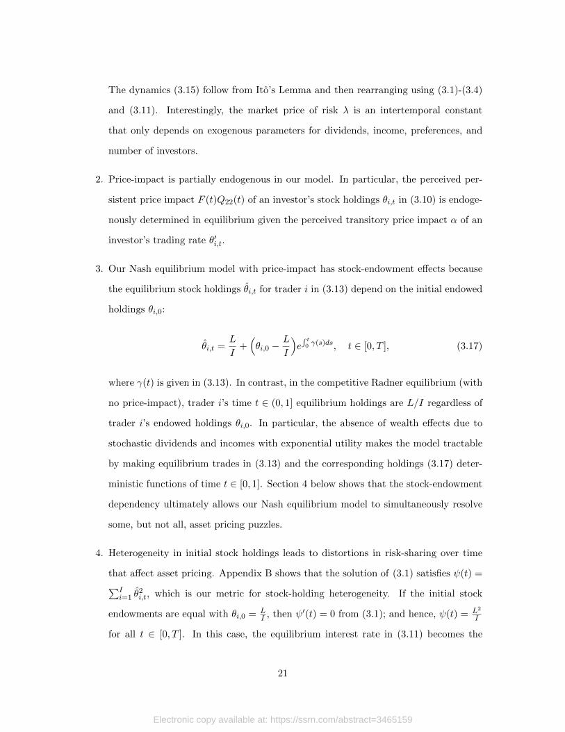
3. Our Nash equilibrium model with price-impact has stock-endowment effects because

the equilibrium stock holdings θi,t for trader i in (3.13) depend on the initial endowed

holdings θi,0:

θi,t =L

I+(θi,0 −

L

I

)e∫ t0 γ(s)ds, t ∈ [0, T ], (3.17)

where γ(t) is given in (3.13). In contrast, in the competitive Radner equilibrium (with

no price-impact), trader i’s time t ∈ (0, 1] equilibrium holdings are L/I regardless of

trader i’s endowed holdings θi,0. In particular, the absence of wealth effects due to

stochastic dividends and incomes with exponential utility makes the model tractable

by making equilibrium trades in (3.13) and the corresponding holdings (3.17) deter-

ministic functions of time t ∈ [0, 1]. Section 4 below shows that the stock-endowment

dependency ultimately allows our Nash equilibrium model to simultaneously resolve

some, but not all, asset pricing puzzles.

4. Heterogeneity in initial stock holdings leads to distortions in risk-sharing over time

that affect asset pricing. Appendix B shows that the solution of (3.1) satisfies ψ(t) =∑Ii=1 θ

2i,t, which is our metric for stock-holding heterogeneity. If the initial stock

endowments are equal with θi,0 = LI , then ψ′(t) = 0 from (3.1); and hence, ψ(t) = L2

I

for all t ∈ [0, T ]. In this case, the equilibrium interest rate in (3.11) becomes the

21


analogous competitive Radner equilibrium interest rate given by (see Appendix C

below):

rRadner := δ −a2σ2

DL2

2I2−a(aIσ2

Y + 2aLρσDσY − 2IµY − 2LµD)

2I. (3.18)

For non-equal endowments (i.e., non-Pareto efficient), Cauchy-Schwarz’s inequality

produces∑I

i=1 θ2i,0 > L2

I , which leads to ψ(t) =∑I

i=1 θ2i,t >

L2

I for all t ∈ [0, T ].

In that case, the Nash equilibrium interest rate (3.11) is strictly smaller than the

competitive Radner equilibrium interest rate in (3.18). Thus, inequality in investor

stock endowments as measured by∑I

i=1 θ2i,t − L2

I is a key quantity in our model’s

ability to resolve the interest rate puzzle and, as shown in Section 4 below, also affects

the stock volatility puzzle. However, over time, the equilibrium holdings in (3.17)

converge to equal holdings (Pareto efficient), and so these asset pricing effects are

temporary.

5. Even if the analogous competitive Radner equilibrium is Pareto-efficient (i.e., if in-

vestor income is spanned), our Nash equilibrium can be non-Pareto efficient. To see

this, set ρ2 = 1 in the income dynamics (2.4), which makes the analogous competitive

Radner model complete. In this case, the interest rate (3.18) in the competitive Rad-

ner equilibrium agrees with the Pareto efficient interest rate given in (D.4) in Appendix

D below. However, as long as θi,0 6= LI for some trader i, we have

∑Ii=1 θ

2i,0 >

L2

I by

Cauchy-Schwarz’s inequality and, consequently, ψ(t) =∑I

i=1 θ2i,t >

L2

I by (3.1). Thus,

even if the competitive Radner equilibrium is Pareto-efficient because ρ2 = 1 in (2.4),

the Nash equilibrium interest rate (3.11) is strictly smaller than the Pareto-efficient

equilibrium interest rate (D.4) whenever θi,0 6= LI for some trader i.

6. Unspanned investor-income randomness also affects risk-sharing and asset pricing.

Individual investor income Yi,t is optimally consumed, as seen in (3.14), and, thus,

income shocks do not directly affect optimal investor holdings. As a result, investor

trading in (3.13) is deterministic, which simplifies the modeling of the stock endow-

22


ment effects. However, the parameters of the investor income process affect asset

pricing in (3.11) and (3.12) and the optimal trading rate θ′i,t in (3.13). Thus, imper-

fect risk-sharing due to both distortions in initial stock endowments and unspanned

(idiosyncratic) shocks to investor income has asset-pricing effects with price-impact.

7. The proof of Theorem 3.3 in Appendix B is based on the standard dynamical program-

ming principle and HJB equations. Thus, by definition, the individual optimization

problems in our Nash equilibrium model are time-consistent. However, it might ap-

pear that our Nash equilibrium model is time-inconsistent given that the optimal

holdings θi,t in (3.17) depend on the endowed holdings θi,0 (see, e.g., the discussion in

Remark 3 on p.455 in Basak, 1997). The explanation for why our Nash equilibrium is

time-consistent while the equilibrium holdings θi,t depend on the endowed holdings θi,0

lies in the state-processes and controls used in the proof of Theorem 3.3, summarized

in Table 1:

Table 1: State-processes and controls used.

State processes Controls

Nash Mi,t, Dt, θi,t ci,t, θ′i,t

Radner and Pareto Xi,t ci,t, θi,t

For time-consistent optimization problems, the initial control values cannot appear in

the optimal controls. However, because the trading rate θ′i,t is the control — not the

stock holdings θi,t — in the Nash equilibrium model, the endowment θi,0 can (and do)

appear in the time-consistent individual optimal holdings θi,t in (3.17). Likewise, the

Radner and Pareto equilibrium models are time-consistent, and so the endowment θi,0

cannot (and do not) appear in the individual optimal holdings LI .

4 Asset-pricing puzzles

This section shows that our continuous-time price-impact equilibrium model produces ma-

terial differences relative to the analogous Radner and Pareto-efficient equilibria. In par-

23


ticular, based on the C-CAPM from Breeden (1979), Appendix D derives the analogous

Pareto-efficient equilibrium where all investors act as price-takers and markets are com-

plete. We show how price-impact affects the three main asset-pricing puzzles (risk-free

rate, equity premium, and volatility). We do this both analytically and by illustrating the

equilibrium differences in a numerical example. The differences between our model and

the Radner and Pareto-efficient equilibria are due to perceived price-impact, heterogenous

stock holdings, and market incompleteness (due to idiosyncratic income risk when ρ2 < 1).

Our conclusion is that, by using the Pareto-efficient equilibrium model as a benchmark,

our price-impact Nash equilibrium model can simultaneously help resolve the risk-free rate

puzzle of Weil (1989), and the volatility puzzle of LeRoy and Porter (1981) and Shiller

(1981). However, price-impact has little quantitative effect on the Sharpe ratio and the

equity premium puzzle of Mehra and Prescott (1985). These empirical works on asset-

pricing puzzles compare a competitive representative agent model with historical data. Such

representative agent models are (effectively) complete and therefore also Pareto efficient by

the First Welfare theorem. Therefore, we use the Pareto efficient equilibrium interest rate

and stock-price process as benchmarks. The comparison with the Radner model shows the

incremental effect of price-impact alone.

4.1 Analytical Comparison

We start by recalling the definition of the equity premium over a time interval [0, t]:

EP(t) : = E

[St − S0 +

∫ t0 Due

∫ tu r(s)dsdu

S0

]−(e∫ t0 r(u)du − 1

), t ∈ [0, T ]. (4.1)

In (4.1), the interest rate r(t) is given in (3.11) with the corresponding (deterministic)

money market account price process is e∫ t0 r(u)du and the equilibrium stock-price process St

is given in (3.12). Based on (4.1), we define the Sharpe ratio measured over a time interval

24


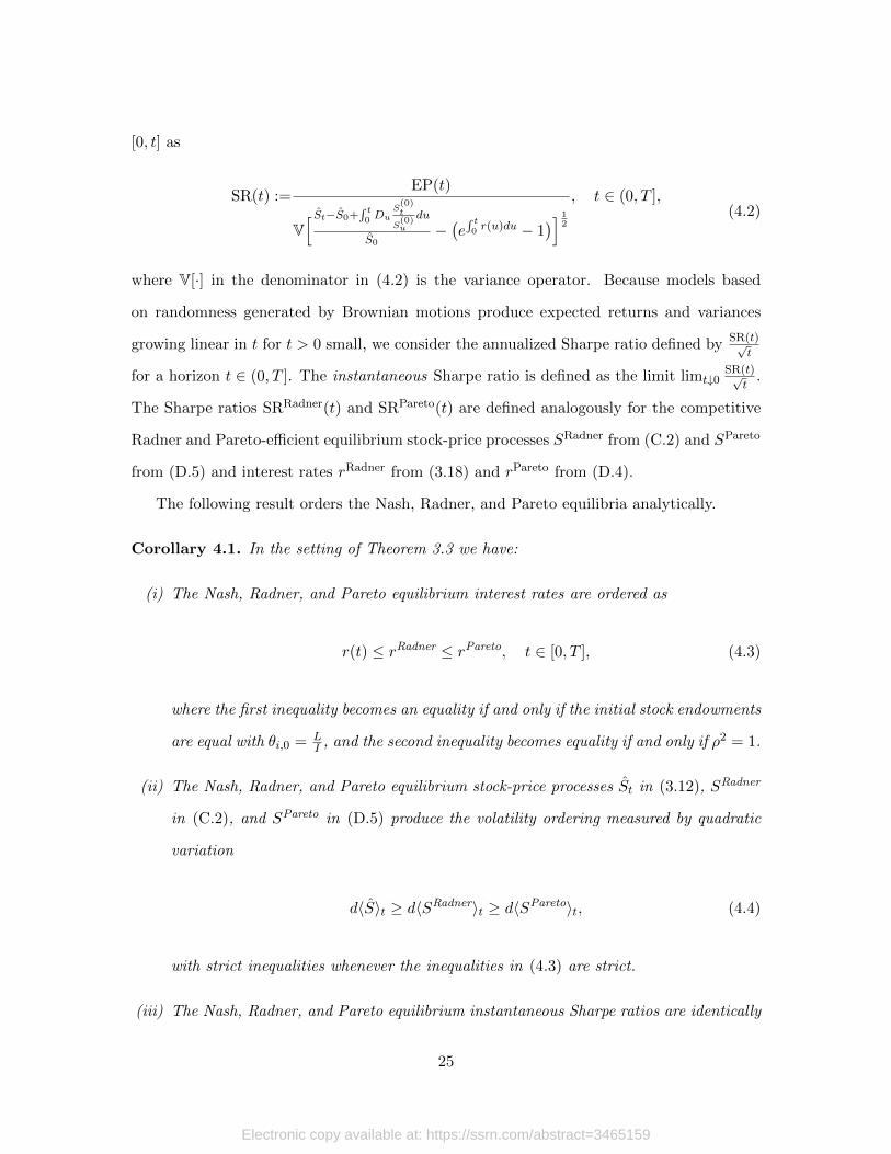
[0, t] as

SR(t) :=EP(t)

V[ St−S0+

∫ t0 Du

S(0)t

S(0)u

du

S0−(e∫ t0 r(u)du − 1

)] 12

, t ∈ (0, T ],(4.2)

where V[·] in the denominator in (4.2) is the variance operator. Because models based

on randomness generated by Brownian motions produce expected returns and variances

growing linear in t for t > 0 small, we consider the annualized Sharpe ratio defined by SR(t)√t

for a horizon t ∈ (0, T ]. The instantaneous Sharpe ratio is defined as the limit limt↓0SR(t)√

t.

The Sharpe ratios SRRadner(t) and SRPareto(t) are defined analogously for the competitive

Radner and Pareto-efficient equilibrium stock-price processes SRadner from (C.2) and SPareto

from (D.5) and interest rates rRadner from (3.18) and rPareto from (D.4).

The following result orders the Nash, Radner, and Pareto equilibria analytically.

Corollary 4.1. In the setting of Theorem 3.3 we have:

(i) The Nash, Radner, and Pareto equilibrium interest rates are ordered as

r(t) ≤ rRadner ≤ rPareto, t ∈ [0, T ], (4.3)

where the first inequality becomes an equality if and only if the initial stock endowments

are equal with θi,0 = LI , and the second inequality becomes equality if and only if ρ2 = 1.

(ii) The Nash, Radner, and Pareto equilibrium stock-price processes St in (3.12), SRadner

in (C.2), and SPareto in (D.5) produce the volatility ordering measured by quadratic

variation

d〈S〉t ≥ d〈SRadner〉t ≥ d〈SPareto〉t, (4.4)

with strict inequalities whenever the inequalities in (4.3) are strict.

(iii) The Nash, Radner, and Pareto equilibrium instantaneous Sharpe ratios are identically

25


given by λ in (3.16); that is,

limt↓0

SR(t)√t

=a

I(LσD + IσY ρ). (4.5)

First, consider the risk-free rate puzzle of Weil (1989). Pareto-efficient equilibrium

models predict interest rates that are too high compared to empirical evidence. From

in (3.11) we see that Nash equilibrium interest rate r(t) is less than both the analogous

competitive interest rate rRadner in (3.18), and the analogous Pareto-efficient interest rate

rPareto in (D.4) in Appendix D. Whenever there is unspanned income risk (i.e., when ρ2 <

1), Christensen, Larsen, and Munk (2012) show that rRadner < rPareto due to a precautionary

saving effect. Here, we find r(t) < rRadner whenever there is stock-endowment inequality

in that θi,0 6= L/I for some trader i ∈ {1, ..., I}.10 The intuition is that price-impact costs

cause investors to rebalance more slowly, which exacerbates risk-bearing inefficiency, which,

in turn, magnifies stock risk and increases bond demand.

Second, consider the volatility puzzle of LeRoy and Porter (1981) and Shiller (1981).

Pareto-efficient models predict a stock-price volatility that is too low compared to empirical

evidence. The ordering (4.3) leads to a reversed annuity ordering:

F (t) ≥ FRadner(t) ≥ FPareto(t), (4.6)

where F (t) is given by the ODE (3.2) and

d

dtFRadner(t) = FRadner(t)rRadner − 1, FRadner(T ) = 1, (4.7)

d

dtFPareto(t) = FPareto(t)rPareto − 1, FPareto(T ) = 1. (4.8)

Consequently, the ordering (4.6) and the equilibrium stock-price processes (3.12), (C.2),

and (D.5) produce the volatility ordering measured by quadratic variation in (4.4). The

intuition is that the multiplication of the current dividend Dt by F (t) in (3.12) represents

10Even without idiosyncratic income risks (i.e., ρ2 = 1 so that rRadner = rPareto), we have r(t) < rRadner.

26


an annuity-valuation effect for the stream of future dividends following Dt at time t. Thus,

lower interest rates in the Nash equilibrium intensify this annuity effect.

Third, consider the equity premium puzzle of Mehra and Prescott (1985). Pareto-

efficient models predict the stock’s excess return over the risk-free rate to be too low

compared to empirical evidence. The equity premium puzzle involves empirical Sharpe

ratios estimated over discrete horizons (e.g., monthly or annually), so the finite-horizon

[0, t] Sharpe ratios SR(t)√t

is the relevant measure. Note here that the finite-horizon Sharpe

ratio (4.2) is a ratio of integrals and not an integral of instantaneous Sharpe ratios. Thus,

finite-horizon Sharpe ratios can differ across the three models (Nash, Radner, and Pareto)

even though their instantaneous Sharpe ratios are identical. However, Section 4.2 below

shows that, over small horizons [0, t] for t > 0, the magnitudes of the finite-horizon Nash

Sharpe ratio are quantitatively similar to the Radner and Pareto Sharpe ratios for a reason-

able set of calibrated model parameters. The reason is that, as t ↓ 0, the time-normalized

discrete-horizon Sharpe ratios in all three models are anchored, by Corollary 4.1, to the

same instantaneous Sharpe ratio λ in (4.5).11 The fact that the Radner and Pareto instan-

taneous Sharpe ratios agree with exponential utilities, continuous-time consumption, and

Brownian motions randomness is proved in Christensen and Larsen (2014, p.273) and is

discussed in Cochrane (2008, p.310). The fact that this is also true for the Nash instanta-

neous Sharpe ratio is a new result. Over longer horizons, our Nash equilibrium model with

price-impact can produce bigger Sharpe ratios (4.2) than the analogous Radner and Pareto

equilibrium models but only for unreasonable parameters. Thus, the calibrated magnitude

of the price-impact Sharpe ratio effect is small.

11There are several ways model incompleteness can produce a different instantaneous Sharpe ratio in thecompetitive (i.e., price-taking) Radner equilibrium model relative to the analogous efficient Pareto model:(i) Traders can be restricted to only consume discretely as in Constantinides and Duffie (1996), (ii) Theunderlying filtration can have jumps as in, e.g., Barro (2006) and Larsen and Sae-Sue (2016), and (iii)Non-time additive utilities as in, e.g., Bansal and Yaron (2004).

27


4.2 Numerics

This section presents calibrated numerics to illustrate the effect of price-impact on all three

asset-pricing puzzles. In our numerics, time is measured on an annual basis (i.e., one year is

t = 1). We normalize the outstanding stock supply to L := 100. As noted in Remark 3.1.3,

the key quantity in explaining the asset pricing puzzles is the heterogeneity in investors’

initial endowments as measured by the difference∑I

i=1 θ2i,0− L2

I ≥ 0 which is a metric for the

distance of the initial stock endowments from Pareto efficiency. To provide some intuition

for this difference, we note that the cross-sectional average and standard deviation of a set

of initial stock endowments ~θ0 := {θ1,0, ..., θI,0} are

mean[~θ0

]: =

1

I

I∑i=1

θi,0

=L

I,

SD[~θ0

]: =

√√√√1

I

( I∑i=1

θ2i,0 −

L2

I

)=

√1

I

(ψ(0)− L2

I

),

(4.9)

where ψ(t) is the function from (3.1).

The utility parameters for (2.10) in our numerics are

δ := 0.02, a := 2. (4.10)

The annual time-preference rate δ is consistent with calibrated time preferences in Bansal

and Yaron (2004), and the level of absolute risk aversion a is from the numerics in Chris-

tensen, Larsen, and Munk (2012). The coefficients for the arithmetic Brownian motion for

the stock dividends in (2.2) are

µD := 0.0201672, σD := 0.0226743, D0 := 1. (4.11)

28


The parameterizations of µD and σD are the annualized mean and standard deviation of

monthly percentage changes in aggregate real US stock market dividends from January

1970 through December 2019 (from Robert Shiller’s website http://www.econ.yale.edu/

~shiller/data.htm). The starting dividend rate D0 = 1 in (4.11) is a normalization.

The annualized income volatility and income-dividend correlation are from the numerics in

Christensen, Larsen, and Munk (2012):

σY = 0.1, ρ = 0. (4.12)

The drift µY and number of investors I ∈ N are found by calibrating the Radner equilibrium

model so that

λ = 0.302324, rRadner = 8.137%, (4.13)

which produces the remaining coefficients12

µY := −0.0709146, I = 15. (4.14)

We set the model horizon T to T := 3 years. In our analysis we found that our numerics

are relatively insensitive to T once T is sufficiently large.

We illustrate that price-impact in the Nash equilibrium can have a material effect on

asset pricing relative to the analogous Pareto-efficient equilibrium. Figure 1 shows interest-

rate and stock return-volatility trajectories over a year t ∈ [0, 1] for the Nash equilibrium

with price-impact, the price-taking Radner equilibrium, and the corresponding Pareto-

efficient equilibrium. For visibility, Figure 1 also shows differences in Sharpe ratios between

the Nash and Radner equilibria since these numerical values are small.

The Nash model with price-impact has two additional parameters relative to the com-

petitive Radner model: The transitory price-impact coefficient α in (3.10) and the difference

12The discount rate δ, dividend parameters µD and σD, and income parameters µY and σY are all quotedin decimal form where 0.01 = 1%.

29


∑Ii=1 θ

2i,t − L2/I = ψ(t) − L2/I for deviations of initial stock endowments from the equal

stock holdings, which is related to the SD[~θ0] in (4.9). Figure 1 illustrates the sensitivity of

asset pricing moments to these two parameters.

Figure 1, Plots A, C, and E show the effects of varying the temporary price-impact

parameter α > 0. Of course, when α > 0 is close to zero, our Nash equilibrium is close to the

Radner equilibrium. In our numerics, we consider two transitory price-impact parameters

of α ∈ {0.01, 0.002}. Appendix E shows that α = 0.002 is roughly consistent with transitory

price-impact estimates in Almgren et al. (2005). To put them in perspective, a price-impact

of α = 0.002 means if an investor trades at a constant rate θ′i = 265 to sell∫ 1

2650 θ′idt = 1

unit of the stock over a day (i.e., a large daily parent trade of 1 percent of L = 100 shares

outstanding), the associated transitory price increase at each time t in the day would be

0.002 × 265 = 0.53. The stock (with α = 0.002 and SD[~θ0] = 5) has an endogenous initial

equilibrium price of S0 = 3.5737, so this corresponds to a sustained percentage transitory

price-impact of 0.002×2653.5737 = 14.83% over the day.

The price-impact feature in the Nash equilibrium can produce up to a 2% annual interest

rate reduction (the reduction is biggest for shorter horizons where, from (3.17), holdings

θi,t differ most from LI ). We see that the stock-return volatility increases by around 0.25%

relative to the Radner volatility. The impact on the Sharpe ratio, while in the right direction

qualitatively, is quantitatively negligible. The Sharpe ratio effects are biggest for longer

horizons. Finally, from Plots A, C, and E, we see that all three asset-pricing impacts are

increasing in the temporary price-impact coefficient α > 0.

Figure 1, Plots B, D, and F consider the effect of different levels of stock-endowment

inequality (SD[~θ0] ∈ {5, 10}). As∑I

i=1 θ2i,0 approaches the calibrated lower bound 1002

15 ≈

666.67 for L2

I from Cauchy-Schwarz’s inequality, the Nash equilibrium converges to the

Radner equilibrium. Plots B, D, and F show all three asset-pricing impacts are increasing

in investor heterogeneity as measured by∑I

i=1 θ2i,0 − L2

I .

The small quantitative effect of price-impact on the equity premium in our analysis is

not due to investor trading incentives being small. To the contrary, the incentive to trade is

30


substantial in these numerical examples: The cross-investor endowment standard deviations

are 5 and 10, relative to the Pareto-efficient stock holdings of 100/15 = 6.66. This suggests

stronger induced trading preferences given other utility specifications may be an important

part of what is needed for price impact to affect the Sharpe Ratio. We leave this to future

research, since exponential preferences are part of the modeling assumptions that make our

current analysis tractable.

31


Figure 1: Trajectories of interest rates (Plots A and B), stock-price volatility (Plots C and

D), and annualized Sharpe ratio differences SR(t)−SRRadner(t)√t

(Plots E and F) for t ∈ [0, 1]

over the first year. The model parameters are given in (4.10), (4.11), (4.12), (4.14), L := 100,T := 3 years, and the time discretization uses 250,000 rounds of trading per year.

0.2 0.4 0.6 0.8 1.0t

-0.02

0.00

0.02

0.04

0.06

0.08

0.10

Interest rate

0.2 0.4 0.6 0.8 1.0t

-0.02

0.00

0.02

0.04

0.06

0.08

0.10

Interest rate

A: SD[~θ0]

:= 5 B: α := 0.002

Nash: α := 0.002 (—–), α := 0.01 (−−), Nash SD[~θ0]

:= 5 (—–), SD[~θ0]

:= 10 (−−),Radner: (− · −), Pareto: (− · ·−) Radner: (− · −), Pareto: (− · ·−)

0.0 0.2 0.4 0.6 0.8 1.0t0.060

0.065

0.070

0.075

0.080Stock volatility

0.0 0.2 0.4 0.6 0.8 1.0t0.060

0.065

0.070

0.075

0.080Stock volatility

C: SD[~θ0]

:= 5 D: α := 0.002

Nash: α := 0.002 (—–), α := 0.01 (−−), Nash: SD[~θ0]

:= 5 (—–),[~θ0]

:= 10 (−−),Radner: (− · −), Pareto: (− · ·−) Radner: (− · −), Pareto: (− · ·−)

0.2 0.4 0.6 0.8 1.0t

0.00002

0.00004

0.00006

0.00008

0.00010Sharpe ratio increase

0.2 0.4 0.6 0.8 1.0t

0.00002

0.00004

0.00006

0.00008

0.00010Sharpe ratio increase

E: SD[~θ0]

:= 5 F: α := 0.002

Nash: α := 0.002 (—–), α := 0.01 (−−) Nash: SD[~θ0]

:= 5 (—–) , SD[~θ0]

:= 10 (−−)

To summarize, Figure 1 shows that price-impact can have a significant impact on inter-

32


est rates and a material impact on stock return volatility for reasonable model parameters.

Moreover, we found that there are model parameterizations such that the quantitative effect

of price-impact on the Sharpe ratio is material in our model. However, these other parame-

terizations involve unrealistically large price-impact and initial stock-holding heterogeneity

and were also associated with unreasonable interest rates. Thus, we conclude that price-

impact in our model only has a negligible impact on the finite-horizon equilibrium Sharpe

ratios. Again, the intuition for this result is the common anchoring of the instantaneous

Sharpe ratio in (4.5).

5 Model extensions

Our analysis has shown how to construct a parsimonious and tractable equilibrium model

of price-impact in continuous-time. However, the following two model extensions illustrate

our Nash equilibrium model’s analytical robustness to variations.

5.1 Discrete-orders

We can allow traders to also place discrete orders (i.e., block trades) as well as consumption

plans with lump sums. To illustrate this, we consider a simple case in which traders can

place block trades and consume in lumps at time t = 0 after which they trade using order

rates and consume using consumption rates for t ∈ (0, T ].

First, we start with block trades and use θi,0− to denote trader i’s initial stock endow-

ment so that ∆θi,0 := θi,0 − θi,0− denotes the block trade at time t = 0. In addition to

(2.11) for t ∈ (0, T ], we conjecture the response at time t = 0 for trader j 6= i to be

∆θj,0 = β0

(F (0)D0 − Si,0

)+ β1θj,0− + β2θi,0− + β3∆θi,0, (5.1)

where (β0, .., β3) are constants (to be determined). The price-impact function trader i

perceives is found using the stock-market clearing condition at time t = 0 when summing

33


(5.1):

0 = (I − 1)β0

(F (0)D0 − Si,0

)+ β1(L− θi,0−)

+ (I − 1)(β2θi,0− + β3∆θi,0

)+ ∆θi,0.

(5.2)

Provided that β0 6= 0, we can solve (5.2) for trader i’s perceived stock market-clearing price

at time t = 0:

Si,0 = D0F (0) +β1L

β0(I − 1)+β2(I − 1)− β1

β0(I − 1)θi,0− +

β3(I − 1) + 1

β0(I − 1)∆θi,0. (5.3)

Second, we introduce time t = 0 lump sum consumption. Because stock prices are

denoted ex dividend, the initial wealth is

Xi,0 = (D0 + Si,0)θi,0− + Yi,0 − Ci, i ∈ {1, ..., I}, (5.4)

where Ci is trader i’s lump sum consumption at time t = 0 (to be determined). The

expression for Xi,0 in (5.4) follows from the normalization that all strategic traders have

zero endowments in the money market account. By using (5.4), the time t = 0 money

market account balance of (2.15) for trader i ∈ {1, ..., I} is given by

Mi,0 :=Xi,0 − Si,0θi,0

=D0θi,0− − Si,0∆θi,0 + Yi,0 − Ci.(5.5)

Next, we show how to modify to the objective in (2.10) to allow for both time t = 0 lump

sum consumption Ci and block trades ∆θi,0. Trader i’s optimization problem becomes:

inf(∆θi,0,Ci)∈R2, (θ′i,ci)∈A

E[e−aCi +

∫ T

0e−aci,t−δtdt+ e−a(Xi,1+Yi,T )−δT

]= inf

(∆θi,0,Ci)∈R2

(e−aCi + v(0,Mi,0, D0, θi,0, Yi,0)

),

(5.6)

where v is the value function defined below in (B.3) in Appendix B corresponding to the

34


objective in (2.10). To minimize the objective in (5.6), we insert Mi,0 from (5.5) and

θi,0 = θi,0− + ∆θi,0 into the last line in (5.6) and minimize to produce the optimal initial

block trade and lump sum consumption. For example, we have

S0 = F (0)(D0 + LQ22(0)

I +Q2(0)),

θi,0 = θi,0− + β1

(θi,0− −

L

I

),

(5.7)

where β1 is a free model parameter (similar to α in Theorem 3.3). From (5.7), we see that

S0 matches the initial stock price in (3.12). Moreover, because of price-impact, we also

see from (5.7) that trader i does not immediately jump to the Pareto efficient holdings LI .

Finally, we note that Corollary 4.1 about the asset pricing effects of price-impact continues

to hold when∑I

i=1 θi,0 is replaced by

I∑i=1

θi,0 =

I∑i=1

(θi,0− + β1

(θi,0− −

L

I

)). (5.8)

5.2 Penalties

In this section our model is extended to allow for inventory penalties and dissipative trans-

action costs. To do this, the objective (2.10) is replaced with

inf(θ′i,ci)∈A

E[∫ T

0e−aci,t−δtdt+ e−a(Xi,1+Yi,T−Li,T )−δT

], i = 1, ..., I, (5.9)

where Li,T is a penalty term. We consider two specifications of Li. First, we can incorporate

high-frequency traders (HFTs) who are incentivized to hold zero positions over time. We

do this by defining the penalty processes:

Li,t :=

∫ t

0κ(s)θ2

i,sds, t ∈ [0, T ], i = 1, ..., I. (5.10)

The deterministic function κ : [0, T ] → [0,∞) in (5.10) is a penalty-severity function. The

strength of κ(t) for t ∈ [0, T ] can vary periodically for times during overnight periods vs

35


during trading days to give HFTs stronger incentive to hold no stocks overnight.

Second, we can approximate deadweight transaction costs by penalizing trading rates

(as in, e.g., Garleanu and Pedersen 2016). We do this by defining the penalty processes:

Li,t :=1

2λ

∫ t

0(θ′i,s)

2ds, t ∈ [0, T ], i = 1, ..., I. (5.11)

The constant λ > 0 in (5.11) is interpreted as a transaction cost parameter.

By altering the ODEs, the existence result in Theorem 3.3 can be modified to include

both penalties (5.10) and (5.11) and linear combinations of (5.10) and (5.11). For this

model extension, the orderings in Corollary 4.1 also continue to hold.

6 Conclusion

This paper has shown, formally and in numerical examples, that price-impact can have

material effects on asset pricing via an amplification effect on imperfect risk sharing. Cali-

brated price-impact helps resolve both the interest rate and volatility puzzles but has only

a negligible quantitative effect on the Sharpe ratios for realistic model parameters.

Our analysis suggests many interesting directions for future work. These include ex-

tending our analysis to non-exponential utility, non-Gaussian dividends, and refinements

of Nash equilibrium for off-equilibrium price perceptions and then investigating whether

such variations relative to our baseline analysis can increase the quantitative effect of price

impact on the Sharpe Ratio.

A Auxiliary ODE result

In the following ODE existence proof, there are no restrictions on the time horizon T ∈

(0,∞) and the constant C0 ∈ R. We note that the ODE (A.3) is quadratic in g(t) and that

the square coefficient − 2α is negative because α > 0 is the temporary price-impact due to

orders θ′i,t.

36


Proposition A.1. For I ∈ N, C0 ∈ R, and positive constants T, a, σD, α, k > 0 there exists

a unique constant h0 ∈ (0, k) such that the ODE system:

h′(t) =2g(t)

αh(t), h(0) = h0, (A.1)

f ′(t) = 1 + f(t)(a2σ2

D2I h(t)− C0

), f(0) = 1, (A.2)

g′(t) = aσ2Df(t)− 2

αg(t)2 + g(t)

(a2σ2

D2I h(t)− C0

), g(0) = 0, (A.3)

with initial condition h0 := h0, has a unique solution for t ∈ [0, T ] that satisfies h(T ) = k.

Proof.

Step 1/3 (h’s range): Let h0 ∈ (0, k) be given. We evolve the ODEs (A.1)-(A.3) from

t = 0 to the right (t > 0). The local Lipschitz property of the ODEs ensure that there

exists a maximal interval of existence [0, τ) with τ ∈ (0,∞] by the Picard-Lindelof theorem

(see, e.g., Theorem II.1.1 in Hartman 2002).

For a constant c, let Tf=c ∈ [0, τ ] be defined as

Tf=c := inf {t ∈ (0, τ) : f(t) = c} ∧ τ, (A.4)

where — as usual — the infimum over the empty set is defined as +∞. We define Tg=c

and Th=c similarly. Suppose that Tf=0 < τ . Then, f(0) = 1 and the continuity of f imply

that f(t) > 0 for t ∈ [0, Tf=0). Since f(Tf=0) = 0, we have f ′(Tf=0) ≤ 0, but (A.2) implies

f ′(Tf=0) = 1 > 0. Therefore, we conclude that

Tf=0 = τ and f(t) > 0 for t ∈ [0, τ). (A.5)

Because g(0) = 0 and g′(0) = aσ2D > 0, we have Tg=0 > 0 and g(t) > 0 for t ∈ (0, Tg=0).

The ODE (A.1) with h(0) = h0 > 0 implies that h(t) increases on the interval [0, Tg=0).

37


Therefore, the ODE (A.2) and the positivity of (f, h) produce

f ′(t) > 1− f(t)C0, t ∈ [0, Tg=0). (A.6)

Then, Gronwall’s inequality produces

f(t) ≥

1+(C0−1)e−C0t

C0if C0 6= 0,

1 + t if C0 = 0.

(A.7)

This inequality implies that

f(t) ≥ C1 for t ∈ [0, Tg=0) where C1 :=

1, if C0 ≤ 1,

1C0, if C0 > 1.

(A.8)

Suppose that Tg=0 < τ . Since g(t) > 0 for t ∈ (0, Tg=0) and g(Tg=0) = 0, we have

g′(Tg=0) ≤ 0. However, this is a contradiction because (A.3) and (A.8) imply g′(Tg=0) ≥

aσ2DC1 > 0 where the positive constant C1 is defined in (A.8).

Up to this point we have shown

Tg=0 = τ and

f(t) ≥ C1 > 0,

h(t) ≥ 0,

g(t) ≥ 0,

for t ∈ [0, τ). (A.9)

To proceed, the positive constant

C2 :=

−αC0

2 , if C0 < 0,

α

(−C0+

√C2

0+4aσ2

DC1

α

)4 , if C0 ≥ 0

(A.10)

38


satisfies

− 2

αx2 − C0x ≥ −

aσ2DC1

2for x ∈ [0, C2]. (A.11)

Because 0 ≤ g(t) < C2 for t ∈ [0, Tg=C2), we can bound (A.3) from below using (A.9) and

(A.11) to see for t ∈ [0, Tg=C2)

g′(t) ≥ aσ2DC1 −

2g(t)2

α− g(t)C0

≥ 1

2aσ2

DC1.

(A.12)

By integrating (A.12) and using the initial condition g(0) = 0 we see g(t) ≥ 12aσ

2DC1t for

t ∈ [0, Tg=C2). Therefore,

Tg=C2 ≤ 2C2

aσ2DC1

. (A.13)

Suppose that Tg=C2 = τ . Then, for t ∈ [0, τ), we have 0 ≤ g(t) < C2 and the ODE

(A.1) produces

h′(t) ≤ 2C2

αh(t),

h(t) ≤ h0 e2C2αt,

(A.14)

where the second inequality uses Gronwall’s inequality. Similarly, for t ∈ [0, τ), the ODE

(A.2) and Gronwall’s inequality imply

f ′(t) ≤ 1 + f(t)(a2σ2

D2I h(t) + |C0|

)≤ 1 + f(t)

(a2σ2

Dh02I e

2C2αt + |C0|

),

f(t) ≤ (1 + t) exp(|C0|t+

a2σ2Dh0α

4IC2(e

2C2αt − 1)

).

(A.15)

The boundedness properties g(t) < C2, (A.14), and (A.15) imply that h, f, and g do not blow

up for t finite. Then, Theorem II.3.1 in Hartman (2002) ensures τ = ∞ which contradicts

39


(A.13). Consequently, we cannot have Tg=C2 = τ and it must be the case that

Tg=C2 < τ. (A.16)

Let Tg=C2 be defined as the first time g reaches C2 strictly after time t = Tg=C2 ; that is,

Tg=C2 := inf{t ∈ (Tg=C2 , τ) : g(t) = C2

}∧ τ. (A.17)

Because g′(Tg=C2) ≥ aσ2DC1

2 > 0 by (A.12), we have

Tg=C2 < Tg=C2 and g(t) > C2 for t ∈ (Tg=C2 , Tg=C2). (A.18)

Suppose that Tg=C2 < τ . Then, g(Tg=C2) = C2 and (A.18) imply that g′(Tg=C2) ≤ 0, but

(A.3), (A.9), and (A.11) produce the contradiction:

g′(Tg=C2) = aσ2Df(Tg=C2)− 2C2

2

α+ C2

(a2σ2

D2I h(Tg=C2)− C0

)≥ aσ2

DC1 −2C2

2

α− C2C0

≥ aσ2DC1

2

> 0.

(A.19)

Therefore, it must be the case that Tg=C2 = τ , which implies the lower bound

g(t) ≥ C2 > 0 for t ∈ [Tg=C2 , τ). (A.20)

Combining (A.12) and (A.20) gives the following global lower bound:

g(t) ≥ aσ2DC1

2 t ∧ C2 for t ∈ [0, τ). (A.21)

In turn, using the ODE (A.1), the bound (A.21) produces the global lower bound for h via

40


Gronwall’s inequality:

h(t) ≥ h0 exp

(2

α

∫ t

0

aσ2DC1

2 s ∧ C2ds

)for t ∈ [0, τ). (A.22)

Next, we suppose Th=k = τ . Then, for t ∈ [0, τ), we have 0 ≤ h(t) < k, and the ODEs

(A.2)-(A.3) and Gronwall’s inequality imply

f ′(t) ≤ 1 + f(t)C3,

f(t) ≤ (1 + t)eC3t,

g′(t) ≤ aσ2Df(t) + g(t)C3

≤ aσ2D(1 + t)eC3t + g(t)C3,

g(t) ≤ aσ2De

C3t(t+ 12 t

2),

(A.23)

where C3 :=a2σ2

D2I k+|C0|. The inequalities in (A.23) and 0 ≤ h(t) ≤ k imply that h, f, and g

do not blow up for t finite. Then, Theorem II.3.1 in Hartman (2002) ensures τ = Th=k =∞.

This is a contradiction because (A.22) implies that h(t) reaches k in finite time. Therefore,

it must be the case that

Th=k < τ. (A.24)

Step 2/3 (Monotonicity): Let 0 < h0 < h0 < k, and denote the solution of the ODE

system (A.1)-(A.3) with the initial condition h(0) = h0 by f , h, and g. The corresponding

maximal existence interval is denoted by τ . We define Tg=g as

Tg=g := inf {t ∈ (0, τ ∧ τ) : g(t) = g(t)} ∧ τ ∧ τ . (A.25)

Because g(0) = g(0) = 0, the ODEs (A.1)-(A.3) have the properties g′(0) = g′(0) = aσ2D

41


and

g′′(0) = aσ2D

(1 +

a2σ2D

I h0 − 2C0

)< aσ2

D

(1 +

a2σ2D

I h0 − 2C0

)= g′′(0).

Therefore,

0 < g(t) < g(t) for t ∈ (0, Tg=g). (A.26)

Suppose that Tg=g < τ ∧ τ . The inequality (A.26) and the ODEs (A.1) and (A.2) imply

that h(t) < h(t)

f(t) < f(t)

for t ∈ (0, Tg=g]. (A.27)

Also, (A.26) and g(Tg=g) = g(Tg=g) produce g′(Tg=g) ≥ g′(Tg=g). However, this contradicts

g′(Tg=g) = aσ2Df(Tg=g)−

2g(Tg=g)2

α+ g(Tg=g)

(a2σ2

D2I h(Tg=g)− C0

)< aσ2

Df(Tg=g)−2g(Tg=g)

2

α+ g(Tg=g)

(a2σ2

D2I h(Tg=g)− C0

)= g′(Tg=g),

(A.28)

where we used (A.3) and (A.27). Therefore, we conclude that Tg=g = τ ∧ τ and

h(t) < h(t)

f(t) < f(t)

g(t) < g(t)

for t ∈ (0, τ ∧ τ). (A.29)

Step 3/3 (Existence): To emphasize the dependence on the initial condition h(0) = h0,

42


we write τ(h0) and Th=k(h0). For example,

Th=k(h0) := inf{t ∈

(0, τ(h0)

): h(t) = k

}∧ τ(h0). (A.30)

Inequality (A.24) in Step 1 implies that Th=k(h0) < ∞ for h0 ∈ (0, k). Step 2 implies

that the map (0, k) 3 h0 7→ Th=k(h0) is strictly decreasing. Therefore, the following three

statements and the Intermediate Value Theorem complete the proof in the sense that we

can choose a unique h0 ∈ (0, k) such that Th=k(h0) = T (recall that T ∈ (0,∞) is the model

time horizon):

(i) limh0↑k Th=k(h0) = 0.

(ii) limh0↓0 Th=k(h0) =∞.

(iii) The map (0, k) 3 h0 7→ Th=k(h0) is continuous.

Here are the proofs of these three statements:

(i) Inequality (A.22) implies (i).

(ii) The inequalities in (A.23) and Gronwall’s inequality produce

h(t) = h0 exp

(∫ t

0

2g(s)α ds

)≤ h0 exp

(∫ t

0

2aσ2De

C3s(s+12 s

2)

α ds

).

(A.31)

Obviously, the function [0,∞) 3 t → exp( ∫ t

0

2aσ2De

C3s(s+12 s

2)

α ds)

is increasing. Therefore,

for any t0 > 0, we can choose h0 > 0 such that

h0 < k exp

(−∫ t

0

2aσ2De

C3s(s+12 s

2)

α ds

), t ∈ [0, t0],

and use (A.31) to see Th=k(h0) > t0. This shows (ii).

(iii) Let h0 ∈ (0, k) be fixed. To emphasize the dependence on the initial condition, we

write(h(t), g(t)

)as(h(t, h0), g(t, h0)

). The local Lipschitz structure of the ODEs (A.1)-

43


(A.3) gives us the continuous dependence of their solutions on the initial condition h0 (see,

e.g., Theorem V.2.1 in Hartman 2002); that is,

limx→h0

h(t, x) = h(t, h0), t ∈[0, τ(h0)

). (A.32)

For 0 < x < h0 we have Th=k(h0) < Th=k(x), and the ODE (A.1) and the Fundamental

Theorem of Calculus produce:

k = h(Th=k(x), x

)= h

(Th=k(h0), x

)+

∫ Th=k(x)

Th=k(h0)

∂∂th(t, x)dt

= h(Th=k(h0), x

)+

2

α

∫ Th=k(x)

Th=k(h0)g(t, x)h(t, x)dt

≥ h(Th=k(h0), x

)+

2x

α

∫ Th=k(x)

Th=k(h0)

(aσ2DC1

2 t ∧ C2

)e

2α

∫ t0

aσ2DC1

2 s∧C2dsdt

≥ h(Th=k(h0), x

)+ xC4

(Th=k(x)− Th=k(h0)

),

(A.33)

where the second last line uses the bounds (A.21) and (A.22) and C4 > 0 is an irrelevant

constant independent of x. Letting x ↑ h0 and using (A.32) produce

limx↑h0

Th=k(x) ≤ Th=k(h0). (A.34)

The opposite inequality trivially holds because Th=k(x) is strictly decreasing. Therefore,

(A.34) holds with equality. Similarly, for x ∈ (h0,k+h0

2 ), we have Th=k(k+h0

2 ) < Th=k(x) <

Th=k(h0) and

h(Th=k(h0), x

)= h

(Th=k(x), x

)+

∫ Th=k(h0)

Th=k(x)

∂∂th(t, x)dt

= k +

∫ Th=k(h0)

Th=k(x)g(t, x)h(t, x)dt

≥ k + xC5

(Th=k(h0)− Th=k(x)

),

(A.35)

44


for a constant C5 independent of x. Letting x ↓ h0 and using (A.32) produce

limx↓h0

Th=k(x) ≥ Th=k(h0). (A.36)

Again, the opposite inequality trivially holds because Th=k(x) is strictly decreasing. There-

fore, (A.36) holds with equality and the continuity property follows.

♦

Proposition A.2. Let h0 = 0 in (A.1). Then, the ODEs (A.1)-(A.3) have unique solutions

on t ∈ [0,∞) with h(t) = 0 for all t ≥ 0.

Proof. As in the proof of Proposition A.1, denote the maximal interval of existence by

(0, τ) for τ ∈ (0,∞]. For t ∈ [0, τ), the solutions to (A.1) and (A.2) are

h(t) = 0,

f(t) =

1+(C0−1)e−C0t

C0if C0 6= 0

1 + t if C0 = 0

.(A.37)

As in the proof of Proposition A.1, we can check that

g(t) ≥ 0 for t ∈ [0, τ). (A.38)

Then (A.3), (A.37), and (A.38) imply that for t ∈ [0, τ),

g′(t) = aσ2Df(t)− 2g(t)2

α − C0g(t)

≤ aσ2Df(t) +

αC20

8 .

(A.39)

Gronwall’s inequality implies that g cannot blow up in finite time. Therefore, we conclude

that τ =∞.

♦

45


B Proof of Lemma 3.2, Theorem 3.3, and Corollary 4.1

Proof of Lemma 3.2. We prove that the coupled ODEs (3.1), (3.2), and (3.4) have unique

solutions for t ∈ [0, T ]. We apply Proposition A.1 and Proposition A.2 with

C0 := δ −a(−2LµD − 2IµY + 2aLρσDσY + aIσ2

Y )

2I−a2σ2

DL2

2I2,

k :=I∑i=1

θ2i,0 −

L2

I,

(B.1)

where k is non-negative by Cauchy-Schwarz’s inequality. The functions

ψ(t) := h(T − t) + L2

I , F (t) := f(T − t), Q22(t) := − g(T − t)f(T − t)

, (B.2)

solve (3.1), (3.2), and (3.4) for t ∈ [0, T ].

From (A.8) in the proof of Proposition A.1, we know that f(t) is bounded away from

zero for t ∈ [0, T ]. Therefore, the solutions to the linear ODEs for Q(t) and Q2(t) in (3.5)

and (3.3) can be found by integration.

♦

Proof of Theorem 3.3.

Step 1/2 (Individual optimality): In this step, we define the function

v(t,Mi, D, θi, Yi) := e−a(MiF (t)

+Dθi+Yi+Q(t)+Q2(t)θi+12Q22(t)θ2i

), (B.3)

for t ∈ [0, T ] and Mi, D, θi, Yi ∈ R. In (B.3), the deterministic functions are defined in

(3.2)-(3.4). We note the terminal ODE conditions produce

v(T,Mi, D, θi, Yi) = e−a(Mi+Dθi+Yi). (B.4)

46


Consequently, because Si,T = DT , we have

e−δT v(T,Mi,T , DT , θi,T , Yi,T ) = e−a(Xi,T+Yi,T )−δT , (B.5)

which is the terminal condition in (2.10). Next, we show that the function e−δtv with v

defined in (B.3) is the value function for (2.10). To see this, let (θ′i, ci) ∈ A be arbitrary. Ito’s

lemma shows that the process e−δtv +∫ t

0 e−aci,u−δudu — with v being shorthand notation

for the process v(t,Mi,t, Dt, θi,t, Yi,t) — has dynamics

d(e−δtv

)+ e−aci,t−δtdt

= e−δtv(ea(−ci,t+Dtθi,t+

Mi,tF (t)

+Q(t)+θi,tQ2(t)+ 12θ2i,tQ22(t)+Y )

−−aα(θ′i,t)

2−aci,t+aDtθi,t+aQ(t)+aθi,tQ2(t)+ 12aθ2i,tQ22(t)+aY−log

(1

F (t)

)+1

F (t)

+aF (t)Q22(t)2(L−θi,tI)2

αI2− aMi,t

F (t)2+

2aθ′i,tQ22(t)(L−θi,tI)I

)dt

− ae−δtv(θi,tσDdBt + σY

(ρdBt +

√1− ρ2dWi,t

)),

(B.6)

where we have used the ODEs (3.1)-(3.4) and the interest rate (3.11). The local martingale

on the last line in (B.6) can be upgraded to a martingale. To see this, we note that θi,t is

bounded and v is square integrable by (2.9) so we can use Cauchy-Schwarz’s inequality to

obtain the needed integrability. Furthermore, to see that the drift in (B.6) is non-negative,

we note the second-order conditions for the HJB equation are (there are no cross terms)

θ′i,t :aα

F (t)> 0,

ci,t : a2e−aci,t > 0.

(B.7)

This first inequality in (B.7) holds because F (t) in (3.2) is the annuity (> 0). Consequently,

the drift in (B.6) is minimized to zero by the controls (3.13) and (3.14). This implies that

e−δtv +∫ t

0 e−aci,u−δudu is a submartingale for all admissible order-rate and consumption

processes θ′i,t and ci,t.

It remains to verify admissibility of the controls (3.13) and (3.14). The explicit solution

47


(3.17) is deterministic and uniformly bounded. Inserting the controls (3.13) and (3.14) into

the money market account balance dynamics (2.16) produces

dMi,t =(r(t)Mi,t + θi,tDt − Stθ′i,t + (Yi,t − ci,t)

)dt

=( log(

1F (t) )

a +Mi,t

(r(t)− 1

F (t)

)−Q(t)

− 1

2θi,t(2Q2(t) + θi,tQ22(t)

)− Stθ′i,t

)dt.

(B.8)

The linear SDE (B.8) has a unique well-defined (Gaussian) solution that satisfies (2.9). All

in all, this shows the admissibility requirements in Definition 2.1 and, hence, optimality of

(3.13) and (3.14) follows from the martingale property of e−δtv +∫ t

0 e−aci,u−δudu.

Step 2/2 (Clearing): Clearly, summing the optimal orders in (3.13) and using∑I

i=1 θi,0 =

L show that the stock market clears for all t ∈ [0, T ]. Summing (3.14) gives us

I∑i=1

ci,t = Ilog(F (t))

a +DtL+ IQ(t) + LQ2(t) +1

2Q22(t)

I∑i=1

θ2i,t +

I∑i=1

Yi,t. (B.9)

Because ψ(0) =∑I

i=1 θ2i,0 and

∑Ii=1 θ

2i,t satisfies the ODE (3.1), we have ψ(t) =

∑Ii=1 θ

2i,t

for all t ∈ [0, T ]. Therefore, the real good market clears if and and only if

0 = Ilog(F (t))

a + IQ(t) + LQ2(t) +1

2Q22(t)ψ(t). (B.10)

The terminal conditions in the ODEs (3.5)-(3.4) ensure clearing holds at time t = T . By

computing time derivatives in (B.10) and using r(t) defined in (3.11), we see that clearing

holds for all t ∈ [0, T ].

Finally, the terminal stock-price condition (2.3) for the equilibrium stock-price process

St in (3.12) holds by the terminal conditions in the ODEs (3.2), (3.3), and (3.4).

♦

Proof of Corollary 4.1:

(i): The expressions in (3.11) and (3.18) imply that the inequality r(t) ≤ rRadner is equivalent

48


to the inequality ψ(t) ≥ L2

I . From the proof of Proposition A.1 and Proposition A.2, we

know that the function h is either strictly positive or identically equal to zero on the interval

[0, T ]. Therefore, the expression for ψ in (B.2) implies that ψ(t) ≥ L2

I . Furthermore,

ψ(t) = L2

I if and only if∑I

i=1 θ2i,0 = ψ(0) = L2

I which — by Cauchy-Schwarz’s inequality —

is equivalent to θi,0 = LI for all 1 ≤ i ≤ I.

By using the expressions in (3.18) and (D.4), we obtain

rPareto − rRadner =a2σ2

Y (1− ρ2)

2

(1− 1

I

)≥ 0. (B.11)

(ii): The equilibrium stock-price processes in (3.12), (C.2), and (D.5) have quadratic vari-

ation processes

d〈S〉t = F (t)2σ2Ddt,

d〈SRadner〉t = FRadner(t)2σ2Ddt,

d〈SPareto〉t = FPareto(t)2σ2Ddt,

(B.12)

where the Nash annuity is given in (3.2) and the Radner and Pareto annuities are defined

as

FRadner(t) :=(rRadner − 1)er

Radner(t−T ) + 1

rRadner, (B.13)

FPareto(t) :=(rPareto − 1)er

Pareto(t−T ) + 1

rPareto. (B.14)

The Radner and Pareto annuities have derivatives (4.7)-(4.8). Therefore, inserting (3.11)

into the Nash annuity (3.2) and using the interest rate ordering (4.3) produce the ordering

(4.6).

49


(iii): To see that (4.5) holds, we write the equity premium (4.1) as

EP(t) =1

S0

(E[St] +

∫ t

0E[Du]e

∫ tu r(s)dsdu

)− e

∫ t0 r(u)du

=F (t)(Q2(t)+L

IQ22(t)

)+F (t)(D0+µDt)+S

(0)t

∫ t0

(D0+µDu)

S(0)u

du

S0− e

∫ t0 r(u)du,

(B.15)

where S(0)t := e

∫ t0 r(u)du. L’Hopital’s rule and the ODEs (3.1)-(3.4) produce the limit

limt↓0

EP(t)

t=aσD(LσD + IρσY )F (0)

IS0

. (B.16)

To compute the numerator in (4.2), we define the function

G(t) :=

∫ t

0

1

S(0)u

du = O(t) as t ↓ 0. (B.17)

Then, we apply Ito’s Lemma to compute the dynamics d(BtG(t)

)which produces the

representation

F (t)Bt + S(0)t

∫ t

0

Bu

S(0)u

du =

∫ t

0

(F (t) + S

(0)t

(G(t)−G(u)

))dBu. (B.18)

Therefore, Ito’s Isometry gives us the variance

V[F (t)Bt + S

(0)t

∫ t

0

Bu

S(0)u

du]

=

∫ t

0

(F (t) + S

(0)t

(G(t) −G(u)

))2du

=

∫ t

0

(F (t)2 + 2F (t)S

(0)t

(G(t) −G(u)

)+ (S

(0)t )2

(G(t)2 − 2G(t)G(u) +G(u)2

))du

= F (t)2t+ 2F (t)S(0)t

(G(t)t−

∫ t

0

G(u)du)

+ (S(0)t )2

(G(t)2t− 2G(t)

∫ t

0

G(u)du+

∫ t

0

G(u)2du)

= F (t)2t+ 2F (t)S(0)t

(O(t)t−O(t2)

)+ (S

(0)t )2

(O(t3) − 2O(t)O(t2) +O(t3)

)= F (t)2t+O(t2).

(B.19)

50


Based on (B.16) and (B.19), the limit in (4.5) equals

limt↓0

SR(t)√t

= limt↓0

S0EP(t)

σD

√tV[F (t)Bt + S

(0)t

∫ t0Bu

S(0)u

du]

= limt↓0

S0EP(t)

σDt√F (t)2 +O(t)

= λ,

(B.20)

where λ is the market price of risk defined in (3.16).

The Radner and Pareto instantaneous Sharpe ratios can be computed similarly.

♦

C Competitive Radner equilibrium

Theorem 2 in Christensen, Larsen, and Munk (2012) shows that there exists a competitive

Radner equilibrium in which the equilibrium interest rate is given by

rRadner = δ +a

I(LµD + IµY )− 1

2

a2

I2

(I2σ2

Y + 2ILρσDσY + L2σ2D

), (C.1)

and the equilibrium stock-price process is given by

SRadnert =

(rRadner − 1)erRadner(t−T ) + 1

rRadnerDt

−(er

Radner(t−T )((rRadner−1)rRadner(t−T )+1)−1)(µD−

aσDI (IρσY +LσD)

)(rRadner)2

.

(C.2)

Ito’s lemma and (C.2) produce the competitive Radner equilibrium stock-price volatility

coefficient of SRadnert to be

(rRadner − 1)erRadner(t−T ) + 1

rRadnerσD. (C.3)

Equivalently, we can write (C.3) as FRadner(t)σD where the Radner annuity FRadner(t) is

given by (4.7).

51


D Pareto efficient equilibrium

The following analysis uses the C-CAPM analysis from Breeden (1979). The utilities (2.10)

produce the representative agent’s utility function as

−e−aIc−δt, c ∈ R, t ∈ [0, T ]. (D.1)

Because the economy’s aggregate consumption is LDt +∑I

i=1 Yi,t, the Pareto efficient equi-

librium model’s unique state-price density ξPareto = (ξParetot )t∈[0,T ] is proportional to the

process

e−aI

(LDt+∑Ii=1 Yi,t)−δt, t ∈ [0, T ]. (D.2)

Ito’s lemma produces the relative state-price dynamics to be:

dξParetot

ξParetot

= −δdt− a

I

(LdDt +

I∑i=1

dYi,t

)+

1

2

a2

I2d〈LD +

I∑i=1

Yi〉t

= −δdt− a

I

((LµD + IµY )dt+ (LσD + IσY ρ)dBt + σY

√1− ρ2

I∑i=1

dWi,t

)+

1

2

a2

I2

((LσD + IσY ρ)2 + Iσ2

Y (1− ρ2))dt.

(D.3)

From (D.3), the Pareto efficient equilibrium’s interest rate (i.e., the dt term in −dξParetot

ξParetot

)

and the market price of risk related to the Brownian motion Bt (i.e., the dBt volatility term

in −dξParetot

ξParetot

) are

rPareto = δ +a

I(LµD + IµY )− 1

2

a2

I2

((LσD + IσY ρ)2 + Iσ2

Y (1− ρ2)),

λ =a

I(LσD + IσY ρ).

(D.4)

52


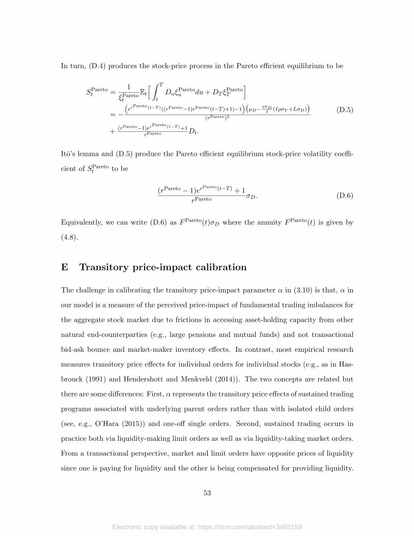
In turn, (D.4) produces the stock-price process in the Pareto efficient equilibrium to be

SParetot =

1

ξParetot

Et[ ∫ T

tDuξ

Paretou du+DT ξ

ParetoT

]= −

(er

Pareto(t−T )((rPareto−1)rPareto(t−T )+1)−1)(µD−

aσDI

(IρσY +LσD))

(rPareto)2

+ (rPareto−1)erPareto(t−T )+1

rPareto Dt.

(D.5)

Ito’s lemma and (D.5) produce the Pareto efficient equilibrium stock-price volatility coeffi-

cient of SParetot to be

(rPareto − 1)erPareto(t−T ) + 1

rParetoσD. (D.6)

Equivalently, we can write (D.6) as FPareto(t)σD where the annuity FPareto(t) is given by

(4.8).

E Transitory price-impact calibration

The challenge in calibrating the transitory price-impact parameter α in (3.10) is that, α in

our model is a measure of the perceived price-impact of fundamental trading imbalances for

the aggregate stock market due to frictions in accessing asset-holding capacity from other

natural end-counterparties (e.g., large pensions and mutual funds) and not transactional

bid-ask bounce and market-maker inventory effects. In contrast, most empirical research

measures transitory price effects for individual orders for individual stocks (e.g., as in Has-

brouck (1991) and Hendershott and Menkveld (2014)). The two concepts are related but

there are some differences: First, α represents the transitory price effects of sustained trading

programs associated with underlying parent orders rather than with isolated child orders

(see, e.g., O’Hara (2015)) and one-off single orders. Second, sustained trading occurs in

practice both via liquidity-making limit orders as well as via liquidity-taking market orders.

From a transactional perspective, market and limit orders have opposite prices of liquidity

since one is paying for liquidity and the other is being compensated for providing liquidity.

53


However, limit buying and market buying both create fundamental asset-holding pressure

on the available ultimate (i.e., non-market-maker) asset sellers. It is the latter that α mea-

sures in our model. Third, stock in our model represents the aggregate stock market as an

asset class and, thus, differs from individual stocks both in terms of its scale and as being a

source of systematic risk rather than also including idiosyncratic stock-specific randomness.

As a result, it seems natural, for example, to measure aggregate trading imbalances relative

to market capitalization (as a measure of fundamental distortions in aggregate asset supply

and demand) rather than in terms of shares (as in a transactional market-maker inventory

model).

Our calibration involves adjusting empirical estimates of transitory price-impact for indi-

vidual stocks into an estimate of the transitory price-impact of trading demand imbalances

for the aggregate market. We proceed as follows: First, rather than using price-impact

measures for individual trades (e.g., as in Hasbrouck (1991)) or market-maker inventory

changes (e.g., as in Hendershott and Menkveld (2014)), we use estimates of the daily tran-

sitory price-impact of parent orders in Almgren, Thum, Hauptmann, and Li (2005). One

advantage of the Almgren et al. (2005) estimation for our purposes is that it measures tran-

sitory price-impacts at the parent order level rather than at the child order level. Another

advantage is that there is a natural way to rescale estimated transitory price-impact for

individual stocks into a price-impact for the aggregate market. In particular, the Almgren

et al. (2005) estimation is an industry-standard approach in which daily price-impact is

estimated given panel data for a sample of parent orders over time for a cross-section of

actively traded stocks. In doing so, the transitory price-impact (TPI) is scaled relative to

a stock’s individual price and daily return volatility and by scaling the underlying parent

order size ∆θ as a percentage relative to a stock’s average daily trading volume (ADV):

TPI

stock price× daily stock return volatility= η ×

( ∆θ

ADV× 100

)β. (E.1)

The coefficient η is estimated in Almgren et al. (2005) to be 0.141, and the exponent

54


β is estimated to be 0.6 (i.e., slightly larger than the standard square-root model). One

final advantage is that these estimates are average effects for all stocks rather than being

driven by stock-specific differences in the trading environment for a particular stock (e.g.,

price level, bid-ask spread, institutional vs. retail ownership, market-maker inventory risk

due to idiosyncratic stock returns). This gives a “dimensionless” standardized measure of

transitory price-impact that can then be rescaled for the aggregate market.

Hence, a preliminary estimate of α in our model is:

TPI ≈ market value × daily market return volatility × η × Qβ3 −Qβ1Q3 −Q1

× SO

ADV× 100

L× θ′i

265

≈ 3.5 × 0.2

√1

265× 0.141 × 1.360.6 − 0.380.6

1.36 − 0.38× 121.36 × 100

100× θ′i

265

≈ 0.0018 × θ′i.

(E.2)

The following steps were used to derive (E.2): First, the market value ($3.50) is set so that

the calibrated absolute (dollar) price-impact is roughly consistent with the stock prices

our asset-pricing model produces. Second, the daily return volatility is set to a ballpark

20% annual return volatility for the aggregate stock market deannualized for one trading

day. Third, the power function in (E.1) is linearized using its slope between the empirical

interquartile values Q1 and Q3 reported in Almgren et al (2005) for the percentage parent-

size/ADV ratio. Fourth, the ratio ∆θADV is factored for our model as SO

ADV∆θSO = 121.36∆θ

L

where 121.36 is the empirical average ratio of shares outstanding to ADV for the NYSE

and Nasdaq for 2009-2018,13 and where shares outstanding SO = L = 100 in our model.

This rescaling measures parent order size relative to shares outstanding, which, as discussed

above, is a natural measure of trade size in our asset-pricing model. Fifth, the parameter

α in (3.10) in our model measures the transitory price-impact relative to the trading rate

θ′i,t (i.e., where θ′i,tdt is the instantaneous child order flow). Thus, we write the daily parent

order ∆θ as

∆θ =

∫ 1265

0θ′idt = θ′i

1

265(E.3)

in terms of a constant child flow rate θ′i over a trading day (i.e., 1265 of a year).

13From the 2019 SIFMQ Capital Market Fact Book.

55


References

[1] Acharya, V. V., and L. H. Pedersen (2005): Asset pricing with liquidity risk, Journal of

Financial Economics 77, 375–410.

[2] Almgren, R. (2003): Optimal execution with nonlinear impact functions and trading-

enhanced risk, Applied Mathematical Finance 10, 1–18.

[3] Almgren, R., C. Thum, E. Hauptmann, and E. Li (2005): Direct estimation of equity

market impact, Risk 18, 58–62.

[4] Amihud, Y., and H. Mendelson (1986): Asset pricing and the bid-ask spread, Journal of

Financial Economics 17, 223–249.

[5] Amihud, Y., H. Mendelson, and L. H. Pedersen (2006): Liquidity and asset prices,

Foundations and Trends in Finance 1, 269–364.

[6] Back, K. (1992): Insider trading in continuous time, Review of Financial Studies 5,

387–409.

[7] Back, K., H. Cao, and G. Willard (2000): Imperfect competition among informed traders,

Journal of Finance 55, 2117–2155.

[8] Baker, M., and J. Wurgler (2006): Investor sentiment and the cross-section of stock

returns, Journal of Finance 61, 1645–1680.

[9] Bansal, R., and A. Yaron (2004): Risks for the long run: A potential resolution of asset

pricing puzzles, Journal of Finance 59, 1481–1509.

[10] Barro, R. J. (2006): Rare disasters and asset markets in the twentieth century, Quarter

Journal of Economics 121, 823–866.

[11] Basak, S. (1996): Dynamic consumption-portfolio choice and asset pricing with non-

price-taking agents, working paper.

[12] Basak, S. (1997): Consumption choice and asset pricing with a non-price-taking agent,

Economic Theory 10, 437–462.

56


[13] Basak, S., and D. Cuoco (1998): An equilibrium model with restricted stock market

participation, Review of Financial Studies 11, 309-341.

[14] Bouchard, B., M. Fukasawa, M. Herdegen, and J. Muhle-Karbe (2018): Equilibrium

returns with transaction costs, Finance and Stochastics 22, 569–601.

[15] Breeden, D. (1979): An inter temporal asset pricing model with stochastic consumption

and investment opportunities, Journal of Financial Economics 7, 265–296.

[16] Brunnermeier, M. K., and L. H. Pedersen (2005): Predatory trading, Journal of Finance

60, 1825–1863.

[17] Calvet, L. E. (2001): Incomplete markets and volatility, Journal of Economic Theory

98, 295–338.

[18] Campbell, J. Y., and J. H. Cochrane (1999): By force of habit: A consumption-based

explanation of aggregate stock market behavior, Journal of Political Economy 107,

205–251.

[19] Campbell, J. Y., S. J. Grossman, and J. Wang (1993): Trading volume and serial

correlation in stock returns, Quarterly Journal of Economics 108, 905–939.

[20] Chien, Y., H. Cole, and H. Lustig (2011): A multiplier approach to understanding the

macro implications of household finance, Review of Economic Studies 78, 199–234.

[21] Choi, J. H., and K. Larsen (2015): Taylor approximation of incomplete Radner equi-

librium models, Finance and Stochastics 19, 653–679.

[22] Choi, J. H., K. Larsen, and D. Seppi (2020): Equilibrium effects of intraday

order-splitting benchmarks, submitted, https://papers.ssrn.com/sol3/papers.

cfm?abstract_id=3146658.

[23] Christensen, P. O., K. Larsen, and C. Munk (2012): Equilibrium in securities markets

with heterogeneous investors and unspanned income risk, Journal of Economic Theory

147, 1035–1063.

57


[24] Christensen, P. O., and K. Larsen (2014): Incomplete continuous-time securities mar-

kets with stochastic income volatility, Review of Asset Pricing Studies 4, 247–285.

[25] Cochrane, J. H. (2005): Asset pricing. Princeton University Press.

[26] Cochrane, J. H. (2008): Financial markets and the real economy, Handbook of the

Equity Risk Premium, 237–325.

[27] Constantinides, G. M., (1986): Capital market equilibrium with transaction costs, Jour-

nal of Political Economy 94, 842–862.

[28] Constantinides, G. M. (1990): Habit formation: A resolution of the equity premium

puzzle, Journal of Political Economy, 98, 519–543.

[29] Constantinides, G. M. (2008): Understanding the equity risk premium puzzle, Hand-

book of the Equity Risk Premium, 331–376.

[30] Constantinides, G. M., and A. Gosh (2017): Asset pricing with countercyclical house-

hold consumption risk, Journal of Finance, 72, 415–460.

[31] Constantinides, G. M., and D. Duffie (1996): Asset pricing with heterogeneous con-

sumers, Journal of Political Economy 104, 219–240.

[32] Coval, J., and E. Stafford (2007): Asset fire sales (and purchases) in equity markets,

Journal of Financial Economics 86, 479–512.

[33] Cvitanic, J., and D. Cuoco (1998): Optimal consumption choices for a large investor,

Journal of Economic Dynamics and Control 22, 401-436.

[34] Duffie, D., Garleanu, N., and L. H. Pedersen (2005): Over the counter markets, Econo-

metrica 73, 1815–1847.

[35] Easley, D., and M. O’Hara (2003): Microstructure and asset pricing, Handbook of the

Economics of Finance 1B, 1021–1051.

[36] Feldman, M., and C. Gilles (1985): An expository note on individual risk without

aggregate uncertainty, Journal of Economic Theory 35, 26–32.

58


[37] Garleanu, N., and L. H. Pedersen (2016): Dynamic portfolio choice with frictions,

Journal of Economic Theory 165, 487–516.

[38] Grossman, S. J., and M. H. Miller (1988): Liquidity and market structure, Journal of

Finance 43, 617–633.

[39] Grossman, S. J., and J. E. Stiglitz (1980): On the impossibility of informationally

efficient markets, American Economic Review 70, 393-408.

[40] Hartman, P. (2002): Ordinary differential equations, 2nd Ed., SIAM Classics in Applied

Mathematics.

[41] Hasbrouck, J. (1991): Measuring the information content of stock trades, Journal of

Finance 46, 179–207.

[42] Heaton, J., and D. Lucas (1992): The effects of incomplete insurance markets and trad-

ing costs in a consumption-based asset pricing model, Journal of Economic Dynamics

and Control 16, 601–620.

[43] Heaton, J., and D. Lucas (1996): Evaluating the effects of incomplete markets on risk

sharing and asset pricing, Journal of Political Economy 104, 443–487.

[44] Hellwig, M. F. (1980): On the aggregation of information in competitive markets, Jour-

nal of Economic Theory 22, 477–498.

[45] Hendershott, T., and A. J. Menkveld (2014): Price pressures, Journal of Financial

Economics 114, 405–423.

[46] Hugonnier, J. (2012): Rational asset pricing bubbles and portfolio constraints, Journal

of Economic Theory 147, 2260–2302.

[47] Judd, K. L. (1985): The law of large numbers with a continuum of iid random variables,

Journal of Economic Theory 35, 19–25.

[48] Kardaras, C., H. Xing, and G. Zitkovic (2015): Incomplete stochastic equilibria with

exponential utilities close to Pareto optimality, working paper.

59


[49] Krueger, D., and H. Lustig (2010): When is market incompleteness irrelevant for the

price of aggregate risk (and when is it not)?, Journal of Economic Theory 145, 1–41.

[50] Kyle, A. (1985): Continuous auctions and insider trading, Econometrica 53, 1315-1336.

[51] Larsen, K., and T. Sae-Sue (2016): Radner equilibrium in incomplete Levy models,

Mathematics and Financial Economics 10, 321–337.

[52] LeRoy, S. F., and R. D. Porter (1981): The present value relation: Tests based on

implied variance bounds, Econometrica 49, 555–574.

[53] Noh, E., and K. Weston (2020): Price impact equilibrium with transaction costs and

TWAP trading, working paper.

[54] Mehra, R., and E. C. Prescott (1985): The equity premium: A puzzle, Journal of

Monetary Economics 15, 145–162.

[55] O’Hara, M. (2015): High frequency market microstructure, Journal of Financial Eco-

nomics, 116, 257–270.

[56] Ohasi, K. (1991): A note on the terminal date security prices in a continuous time

trading model with dividends, Journal of Mathematical Economics 20, 219–224.

[57] Ohasi, K. (1992): Corrigendum: A note on the terminal date prices in a continuous

time trading model with dividends, Journal of Mathematical Economics 21, 199.

[58] Pritsker, M. (2009): Large investors: Implications for equilibrium asset returns, shock

absorption, and liquidity, working paper.

[59] Sannikov, Y., and A. Skrzypacz (2016): Dynamic trading: Price inertia and front-

running, working paper, Stanford University Graduate School of Business.

[60] Schied, A., and T. Schoneborn (2009): Risk aversion and the dynamics of optimal

liquidation strategies in illiquid markets, Finance Stochastics 13, 181–204.

[61] Shiller, R. J. (1981): Do stock prices move too much to be justified by subsequent

changes in dividends?, American Economic Review 71, 421–436.

60


[62] Stoll, H. R. (1978): The pricing of security dealer services: An empirical study of

NASDAQ stocks, Journal of Finance 33, 1153–1172.

[63] Storesletten, K., C. Telmer, and A. Yaron (2007): Asset pricing with idiosyncratic risk

and overlapping generations, Review of Economic Dynamics 10, 519–548.

[64] Storesletten, K., C. Telmer, and A. Yaron (2008): Asset prices and intergenerational

risk sharing: The role of idiosyncratic earnings shocks. Handbook of the Equity Risk

Premium, 565–590.

[65] Townsend, R. M. (1983): Forecasting the forecasts of others, Journal of Political Econ-

omy 91, 546–588.

[66] Uhlig, H. (1996): A law of large numbers for large economies, Economic Theory 8,

41–50.

[67] Vayanos, D. (1999): Strategic trading and welfare in a dynamic market, Review of

Economic Studies 66, 219–254.

[68] Vayanos, D. (2001): Strategic trading in a dynamic noisy market, Journal of Finance

56, 131–171.

[69] Vayanos, D., and J.-L. Vila (1999): Equilibrium interest rate and liquidity premium

with transaction costs, Economic Theory 13, 509–539.

[70] Wachter, J. A. (2013): Can time-varying risk of rare disasters explain aggregate stock

market volatility?, Journal of Finance 68, 987–1035.

[71] Wang, N. (2003): Caballero meets Bewley: The permanent-income hypothesis in gen-

eral equilibrium, American Economic Review 93, 927–936.

[72] Weil, P. (1989): The equity premium puzzle and the risk-free rate puzzle, Journal of

Monetary Economics 24, 401–421.

[73] Weston, K. (2018): Existence of a Radner equilibrium in a model with transaction

costs, Mathematics and Financial Economics 12, 517–539.

61


[74] Weston, K., and G. Zitkovic (2020): An incomplete equilibrium with a stochastic an-

nuity, Finance and Stochastics 24, 359–382.

[75] Zitkovic, G. (2012): An example of a stochastic equilibrium with incomplete markets,

Finance and Stochastics 16, 177–206.

62


Asset-pricing puzzles and price-impact∗ - American ...

Documents

Transcript of Asset-pricing puzzles and price-impact∗ - American ...