NBER WORKING PAPER SERIES

INCOMPLETE MARKET DYNAMICS INNEOCLASSICAL PRODUCTION ECONOMY

George-Marios AngeletosLaurent-Emmanuel Calvet

Working Paper 11016http://www.nber.org/papers/w11016

NATIONAL BUREAU OF ECONOMIC RESEARCH1050 Massachusetts Avenue

Cambridge, MA 02138December 2004

We received helpful comments from P. Aghion, A. Banerjee, R. Barro, J. Benhabib, R. Caballero, O. Galor,J. Geanakoplos, J.M. Grandmont, O. Hart, A. Kajii, H. Polemarchakis, K. Shell, R. Townsend, and seminarparticipants at Brown, Harvard, Maryland, MIT, NYU, Yale, and the 2004 GETA Conference at KeioUniversity. The paper also benefited from excellent research assistance by Ricardo Reis. The viewsexpressed herein are those of the author(s) and do not necessarily reflect the views of the National Bureauof Economic Research.

© 2004 by George-Marios Angeletos and Laurent-Emmanuel Calvet. All rights reserved. Short sections oftext, not to exceed two paragraphs, may be quoted without explicit permission provided that full credit,including © notice, is given to the source.

Incomplete Market Dynamics in a Neoclassical Production EconomyGeorge-Marios Angeletos and Laurent-Emmanuel CalvetNBER Working Paper No. 11016December 2004JEL No. D51, D52, D92, E20, E32

ABSTRACT

We investigate a neoclassical economy with heterogeneous agents, convex technologies and

idiosyncratic production risk. Combined with precautionary savings, investment risk generates rich

effects that do not arise in the presence of pure endowment risk. Under a finite horizon, multiple

growth paths and endogenous fluctuations can exist even when agents are very patient. In infinite-

horizon economies, multiple steady states may arise from the endogeneity of risktaking and interest

rates instead of the usual wealth effects. Depending on the economy's parameters, the local dynamics

around a steady state are locally unique, totally unstable or locally undetermined, and the equilibrium

path can be attracted to a limit cycle. The model generates closed-form expressions for the

equilibrium dynamics and easily extends to a variety of environments, including heterogeneous

capital types and multiple sectors.

George -Marios AngeletosDepartment of EconomicsMIT50 Memorial Drive, E51-251Cambridge, MA 02142and NBERangelet@mit.edu

Laurent-Emmanuel CalvetDepartment of EconomicsHarvard UniversityCambridge, MA 02138and NBERlaurent_clavet@harvard.edu

1 Introduction

How does incomplete risk-sharing affect the level and volatility of macroeconomic activity? We

investigate this question in a neoclassical economy with missing markets and decentralized produc-

tion. Idiosyncratic technological risks, unlike endowment shocks, introduce private risk premia on

capital investment. The interaction of these premia with the precautionary motive can generate

endogenous fluctuations and multiple equilibria even when agents are very patient, technology is

strictly convex, and the wealth distribution has no effect on endogenous aggregates.

We conduct the analysis in the GEI growth framework introduced in Angeletos and Calvet

(2003). Each agent is both a consumer and a producer, who can invest in a private neoclassical

technology with diminishing returns to scale. In contrast to the traditional Ramsey model, individ-

uals are exposed to idiosyncratic shocks in productive investment and possibly in some exogenous

endowment. Agents also trade in financial markets. They can borrow or lend a risk-free bond,

and partially hedge their idiosyncratic risks by exchanging a finite number of risky assets. All

securities are real and there are no constraints on short sales. When markets are complete, the

economy reduces to a Ramsey growth model with identical agents, as in Cass (1965), Koopmans

(1965), and Brock and Mirman (1972). With missing markets, on the other hand, the economy

cannot be described by a representative agent; explicit aggregation is nonetheless possible under a

CARA-normal specification for preferences and risks.

We previously established two main results on macroeconomic performance in the neighbor-

hood of complete markets. First, idiosyncratic production shocks, unlike endowment risk, tend to

discourage investment. Thus in contrast to Bewley models (e.g. Aiyagari, 1994; Huggett, 1997;

Krusell and Smith, 1998), incomplete risk-sharing can lead to lower steady state levels of capital

and output than under complete markets.1 Second, financial incompleteness can increase the per-

sistence of the business cycle. In the traditional Ramsey framework, a negative wealth shock has

some persistence because agents seek to smooth consumption through time. When markets are

incomplete, productive investment is risky and becomes even less attractive relative to current con-

sumption. This can slow down convergence to the steady state, and thus increase the persistence

of aggregate shocks.

The present paper extends our earlier work in a number of useful directions, including high levels

of financial incompleteness and finite-horizon economies. We show that idiosyncratic production

risk can generate rich dynamics that cannot be generated by endowment risks.

We begin by investigating finite-horizon economies. In contrast to the complete market Ramsey

model, agents accumulate large precautionary wealth in later periods, because shocks received

around the terminal date cannot be smoothed through time by borrowing and lending. In economies

1See Ljungqvist and Sargent (2000) for an excellent discussion of Bewley models.

1

with large uninsurable risks, the anticipation of these movements lead to endogenous fluctuations

along the entire equilibrium path.

The interaction between investment risk and precautionary savings can also generate non-

monotonicities in the equilibrium recursion. As a result, there exist multiple growth paths in

some economies with investment risks.

We next examine infinite horizon economies. Multiple steady states can then arise from idiosyn-

cratic production risks and the endogeneity of interest rates. Under incomplete markets, individual

risk-taking is encouraged by the ability to self-insure against future consumption shocks, and thus

by the anticipation of low borrowing rates in later periods. This property can generate multiple

steady states in infinite horizon economies. In a rich equilibrium, a low real interest rate encourages

a high level of risk-taking and investment, which in turn implies a low marginal productivity of

capital and therefore a low interest rate. Conversely in a poor steady state or poverty trap, high

real interest rates, high private risk premia and low investment are self-sustained. Poverty traps

thus originate from the interaction between borrowing costs and risk-taking, a source of multiplicity

that, to the best of our knowledge, is new to the literature. In contrast, earlier work has obtained

poverty traps from wealth effects, building on the idea that poorer agents have lower ability to

borrow and invest and may thus be trapped at low wealth levels (e.g., Banerjee and Newman,

1991; Galor and Zeira, 1993). We eliminate wealth effects by assuming CARA preferences, and

highlight another channel through which financial incompleteness may affect the development of

an economy: the impact of real interest rates on risk-taking.

The local dynamics around the steady state have a rich structure under incomplete markets.

Depending on the economy’s parameters, a steady state is locally unique, totally unstable or lo-

cally undetermined, and the equilibrium path can be attracted to a limit cycle. We observe that

the complicated dynamics arise even when agents are very patient. This suggests that financial

incompleteness may help mitigate the role of heavy discounting in neoclassical growth models of en-

dogenous cycles (e.g. Boldrin and Montrucchio, 1986).2 For instance, Mitra (1996) and Nishimura

and Yano (1996) prove that a period-three cycle only exists if the discount factor β is less than

the constant [(√5 − 1)/2]2 ≈ 0.38. By contrast, our GEI growth economy generates determinis-

tic fluctuations with a Cobb-Douglas technology for large values of the discount factor, such as

β = 0.95.

We observe that like in finite horizon case, complicated dynamics arise even though technology

is convex and there are no credit constraints. Our results thus complements earlier work examining

how equilibrium multiplicity and endogenous cycles may originate from production non-convexities

(e.g. Benhabib and Farmer, 1994), overlapping generations (Benhabib and Day, 1982; Grandmont,

2Note that it is possible to observe fluctuations in a multi-sector growth model for more patient agents (Benhabib

and Nishimura, 1979).

2

1985) or credit constraints (Galor and Zeira, 1993; Kiyotaki and Moore, 1997; Aghion, Banerjee and

Piketty, 1999; Aghion, Bacchetta and Banerjee, 2000). The paper also extends the results obtained

in the incomplete-markets endowment economy of Calvet (2001). Idiosyncratic production risks,

unlike endowment risks, generate cycles even though storage and productive capital can be used as

smoothing devices. They also induce novel dynamic effects, such a complementarity between future

and current investment, and a negative feedback between future capital and current consumption.

Finally, we show that the tractability of our framework is preserved under a number of ex-

tensions. For instance, we introduce a storage technology with fixed positive returns, as well as

randomness in the depreciation of productive capital. The model also generalizes to physical and

human capital, and multiple sectors. Idiosyncratic production risks then also affect the alloca-

tion of savings across different types of capital or different sectors, thus introducing additional

inefficiencies.

Section 2 presents the model. We solve the individual decision problem and calculate the

equilibrium path under a finite horizon in Section 3. In Section 4 we investigate the infinite-horizon

economy and examine the comparative statics and local dynamics of the steady state. Extensions

to multiple capital types and sectors are considered in section 5. We conclude in Section 6. Unless

stated otherwise, all proofs are given in the Appendix.

2 The Model

We consider a neoclassical growth economy with a finite number of heterogeneous agents, indexed

by h ∈ 1, ...H. Agents are born at date t = 0, and live and consume a single good in dates

t ∈ 0, 1, .., T. The horizon is either finite (T <∞) or infinite (T =∞). The economy is stochasticand all random variables are defined on a probability space (Ω,F ,P).

2.1 Production and Idiosyncratic Risks

Each individual is an entrepreneur who owns his own stock of capital and operates his own pro-

duction scheme. The technology is standard neoclassical, convex, and requires neither adjustment

costs nor indivisibilities in investment. These assumptions would lead to the standard neoclassical

growth model, if it were not for the following: production is subject to (partially undiversifiable)

idiosyncratic uncertainty. An investment of kht units of capital at date t yields

yht+1 = Aht+1F (k

ht ) + (1− δht+1)k

ht

units of the consumption good at date t + 1. The production function F is increasing, strictly

concave, and satisfies the Inada conditions.3 The total factor productivity Aht+1 and the depreciation

3The function F satisfies F 0 > 0, F 00 < 0, F (0) = 0, F 0(0) = +∞, F (+∞) = +∞, and F 0(+∞) = 0.

3

rate δht+1 are random shocks specific to individual h, which introduce investment risk. They are

the key ingredients of the model.

The productivity shocks (Aht+1, δ

ht+1) allow us to capture the impact on growth of a wide range

of technological risks. The uncertainty of an entrepreneurial project obviously influences specific

investment in capital or R&D. More generally, the riskiness of a worker’s human capital affects a

wide range of decisions such as labor supply,4 education, learning-by-doing, job search and career

choices. As will be seen in Section 5, the model can be conveniently extended to explicitly include

multiple sectors or the accumulation of human and physical capital.

For comparison purposes, we introduce two additional sources of income. First, individuals

have access to a linear storage technology with gross rate of return ρ ∈ [0, 1]. An investment ofsht units of the good yields ρs

ht with certainty at date t + 1. Second, agents receive an exogenous

stochastic endowment stream eht Tt=0. Income eht+1 captures the effect of risks that are outside thecontrol of individuals and do not affect production capabilities. Like productivity and depreciation,

exogenous income eht+1 is unknown at t and revealed at t+ 1.

2.2 Asset Structure and Preferences

Individual risks can be partially hedged by trading a limited set of real securities. Each asset

n ∈ 0, ..,N is short-lived: it is worth πn,t units of the good at date t, and yields dn,t+1 units of

the good at date t+1. Security n = 0 is riskless and delivers d0,t+1 ≡ 1 with certainty next period.The quantity Rt ≡ 1/π0,t denotes the gross interest rate between t and t + 1, and rt = Rt − 1 isthe corresponding net rate. Assets are in zero net supply, there are no short-sale constraints, and

default is not allowed. It is convenient to stack asset prices and payoffs into the vectors

πt = (πn,t)Nn=0 and dt+1 = (dn,t+1)

Nn=0.

Without loss of generality, we assume that (dn,t+1)Nn=0 is an orthonormal family of L2(Ω), implying

that risky assets have zero expected payoffs and are mutually uncorrelated.

At the outset of every period t, investors are informed of the realization of the asset payoffs dt and

idiosyncratic shocks (Aht , δ

ht , e

ht )Hh=1. Information is thus symmetric across agents.5 Conditional

on available information, agent h selects a portfolio θht = (θhn,t)

Nn=0 in period t.

We assume by construction that all the assets traded in one period are short-lived, in the sense

that they only deliver payoffs in the next period. In the next sections, we will focus on equilibria with

zero risk premia and deterministic interest rate sequences Rt0≤t<T . For this reason, equilibrium4See Marcet, Obiols-Homs and Weil (2000) for a recent discussion of the labor supply in a Bewley model.5The results of this paper would not be modified under the weaker assumptions that income shocks are privately

observed and the structure of the economy is common knowledge (provided of course that the financial structure

remains exogenous).

4

allocations and prices do not change if we introduce a perpetuity, namely a security delivering one

unit of the good every period.6 The perpetuity is worth Πt =PT−1

s=t 1/(Rt...Rs) at date t after

delivery of the period’s coupon.

Each agent maximizes expected lifetime utility Uh0 = E0

PTt=0 β

tu(cht ) subject in all date-events

to the budget constraints

cht + kht + sht + πt · θht = wht (1)

wht+1 = eht+1 +Ah

t+1F (kht ) + (1− δht+1)k

ht + ρsht + dt+1 · θht (2)

The variable wht , called wealth, represents the trader’s net financial position at date t. When the

horizon T is finite, we use the convention that shT = 0 and θhT = 0. Under an infinite horizon, we

instead impose the transversality condition limt→∞ E0βtu(wht ) = 0.

2.3 CARA-Normal Specification

Agents have identical exponential utilities

u(c) = − 1Γexp(−Γc),

where Γ > 0 is the coefficient of absolute risk aversion. The asset payoffs dt+1 and idiosyncratic

shocks ¡Aht+1, δ

ht+1, e

ht+1

¢h are jointly normal and independent of past information. There is thus

no distinction between the conditional and unconditional distribution of these variables. The (un-

conditional) distribution of payoffs and shocks can vary through time, which in future applications

may prove useful to capture the dynamic effect of financial innovation or business cycle variations

in uninsurable risk (e.g. Mankiw, 1986; Constantinides and Duffie, 1996).

We obtain a tractable model when investment opportunities are symmetric across agents and

idiosyncratic shocks cancel out in the aggregate. Specifically, we assume that the mean of idiosyn-

cratic shocks is both constant and homogeneous across the population:

A ≡ EAht+1 > 0, δ ≡ Eδht+1 ∈ [0, 1], e ≡ Eeht+1 ≥ 0.

We rule out aggregate risk by imposing in every period the cross-sectional restriction:

1

H

HXh=1

⎡⎢⎢⎣Aht+1

δht+1

eht+1

⎤⎥⎥⎦ =⎡⎢⎢⎣

A

δ

e

⎤⎥⎥⎦ .This assumption implies that the endogenous fluctuations observed in equilibrium will be unrelated

to aggregate shocks.

6More generally, traders can dynamically replicate a large class of long-lived risky assets.

5

Finally, we must guarantee that idiosyncratic risk is symmetrically distributed across the pop-

ulation. For all h, project the idiosyncratic risks on the asset span available at date t:

Aht+1 = A+

PNn=1 β

h,tA,ndn,t+1 +

eAht+1,

δht+1 = δ +PN

n=1 βh,tδ,ndn,t+1 +

eδht+1,eht+1 = e+

PNn=1 β

h,te,ndn,t+1 + eeht+1.

The residuals ( eAht+1;

eδht+1; eeht+1) represent the undiversifiable component of the investment and en-dowment shocks to individual h. We assume that they are mutually uncorrelated:⎡⎢⎢⎣

eAht+1eδht+1eeht+1

⎤⎥⎥⎦ ∼ N⎛⎜⎜⎝0,

⎡⎢⎢⎣σ2A,t+1 0 0

0 σ2δ,t+1 0

0 0 σ2e,t+1

⎤⎥⎥⎦⎞⎟⎟⎠ ,

and that the standard deviations σt+1 = (σA,t+1;σδ,t+1;σe,t+1) are identical for all agents. The com-

ponents of σt+1 represent useful measures of financial incompleteness, which can deterministically

vary through time.

The CARA-normal specification will ensure that, given a deterministic price sequence, aggregate

quantities are independent of the wealth distribution. This will overcome the curse of dimensionality

that arises when the distribution of wealth — an infinite-dimensional object — enters the state space

of the economy.

2.4 Equilibrium

Given a price sequence πtTt=0, each agent chooses an adapted contingent plan cht , kht , sht , θht , wht Tt=0.

Definition. A GEI equilibrium consists of a price sequence πtTt=0 and a collection of individualplans (cht , kht , sht , θht , wh

t Tt=0)1≤h≤H such that:

(i) Given prices, each agent’s plan is optimal.

(ii) Asset markets clear in every date-event:PH

h=1 θht = 0.

We make two immediate observations. First, if Rt < ρ, agents want to borrow an infinite amount at

rate Rt and invest it in the storage technology. The absence of arbitrage thus requires that Rt ≥ ρ

in any date-event. Second, the absence of aggregate risk in the CARA-normal framework implies

that deterministic price sequences πtTt=0 can be obtained in equilibrium. We henceforth focus onprice sequences satisfying these two conditions.

6

3 Equilibrium under a Finite Horizon

3.1 Decision Theory

Consider an exogenous, deterministic path of asset prices πtTt=0 satisfying the no-arbitrage con-dition Rt ≥ ρ in every period. We focus on a fixed agent h and denote by Jh(w, t) her indirect

utility of wealth along the price path as of date t. Indirect utility satisfies the Bellman equation:

Jh(wht , t) = max

cht ,kht ,sht ,θht u (c) + βEtJh(wh

t+1, t+ 1)

subject to the budget constraints (1) and (2). Since Jh (w,T ) ≡ u(w) at the terminal date, the

value functions Jh (., t) can be solved by a backward recursion.

The results are conveniently presented using

Φ(k) ≡ AF (k) + (1− δ)k + e,

G(k, a, σ) ≡ Φ(k)− Γa[F (k)2σ2A + k2σ2δ + σ2e]/2.

The function Φ(k) denotes the expected non-financial wealth when investing k units of capital. In

contrast, G(k, a, σ) is the risk-adjusted level of non-financial wealth corresponding to productive

investment k, marginal propensity to consume next period a, and residual risks σ = (σA, σδ, σe) .

Lemma 1 The value function belongs to the CARA class in every period:

Jh(w, t) = −(Γat)−1 exp[−Γ(atw + bht )].

The coefficients at and bht are defined recursively by the terminal conditions aT = 1, bhT = 0, and

the equations

at =1

1 + (at+1Rt)−1, (3)

bht = at

ÃMh

t +bht+1

at+1Rt

!, (4)

where

Mht =

G(kht , at+1, σt+1)

Rt− kht −

ln(βRt)

Γat+1Rt+

NXn=1

πn,t

∙βh,te,n + βh,tA,nF (k

ht )− βh,tδ,nk

ht +

Rtπn,t2Γat+1

¸. (5)

The optimal capital stock satisfies

kht ∈ argmaxk≥0

(G(k, at+1, σt+1)−Rtk +Rt

NXn=1

πn,t[βh,tA,nF (k)− βh,tδ,nk]

), (6)

7

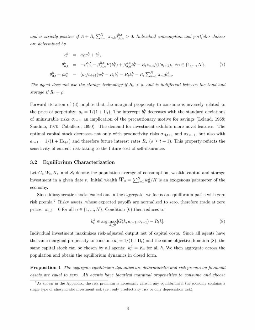
and is strictly positive if A + RtPN

n=1 πn,tβh,tA,n > 0. Individual consumption and portfolio choices

are determined by

cht = atwht + bht ,

θhn,t = −βh,te,n − βh,tA,nF (kht ) + βh,tδ,nk

ht −Rtπn,t/(Γat+1), ∀n ∈ 1, ..., N,

θh0,t + ρsht = (at/at+1)wht −Rtb

ht −Rtk

ht −Rt

PNn=1 πn,tθ

hn,t.

(7)

The agent does not use the storage technology if Rt > ρ, and is indifferent between the bond and

storage if Rt = ρ

Forward iteration of (3) implies that the marginal propensity to consume is inversely related to

the price of perpetuity: at = 1/(1 + Πt). The intercept bht decreases with the standard deviations

of uninsurable risks σt+1, an implication of the precautionary motive for savings (Leland, 1968;

Sandmo, 1970; Caballero, 1990). The demand for investment exhibits more novel features. The

optimal capital stock decreases not only with productivity risks σA,t+1 and σδ,t+1, but also with

at+1 = 1/(1 + Πt+1) and therefore future interest rates Rs (s ≥ t + 1). This property reflects the

sensitivity of current risk-taking to the future cost of self-insurance.

3.2 Equilibrium Characterization

Let Ct,Wt,Kt, and St denote the population average of consumption, wealth, capital and storage

investment in a given date t. Initial wealth W 0 =PH

h=1wh0/H is an exogenous parameter of the

economy.

Since idiosyncratic shocks cancel out in the aggregate, we focus on equilibrium paths with zero

risk premia.7 Risky assets, whose expected payoffs are normalized to zero, therefore trade at zero

prices: πn,t = 0 for all n ∈ 1, ...,N. Condition (6) then reduces to

kht ∈ argmaxk≥0

[G(k, at+1, σt+1)−Rtk]. (8)

Individual investment maximizes risk-adjusted output net of capital costs. Since all agents have

the same marginal propensity to consume at = 1/(1+Πt) and the same objective function (8), the

same capital stock can be chosen by all agents: kht = Kt for all h. We then aggregate across the

population and obtain the equilibrium dynamics in closed form.

Proposition 1 The aggregate equilibrium dynamics are deterministic and risk premia on financial

assets are equal to zero. All agents have identical marginal propensities to consume and choose

7As shown in the Appendix, the risk premium is necessarily zero in any equilibrium if the economy contains a

single type of idiosyncratic investment risk (i.e., only productivity risk or only depreciation risk).

8

identical levels of investment. Macroeconomic aggregates satisfy in every period t the recursion

Kt ∈ argmaxk≥0

[G(k, at+1, σt+1)−Rtk]. (9)

Wt+1 = Φ(Kt) + ρSt (10)

at = 1/[1 + (at+1Rt)−1] (11)

Ct+1 − Ct = ln(βRt)/Γ+ Γa2t+1

£F (Kt)

2σ2A,t+1 +K2t σ

2δ,t+1 + σ2e,t+1

¤/2 (12)

Wt = Ct +Kt + St (13)

and the boundary conditions W0 =W 0, aT = 1 and KT = 0.

While individuals are subjected to idiosyncratic shocks, macroeconomic quantities are deterministic

functions of time. Nevertheless, the economy cannot be represented by a representative agent with

consumption flow Ct, because equilibrium investment (6) and consumption growth (12) depend

on idiosyncratic risk.

Mean consumption growth increases with the variance of future individual consumption, V art(cht+1)

= a2t+1[F (Kt)2σ2A,t+1+K2

t σ2δ,t+1+σ2e,t+1], which is a familiar consequence of the precautionary mo-

tive. The optimal capital stock, on the other hand, satisfies the FOC:

Rt = 1− δ +AF 0(Kt)− Γat+1[F (Kt)F0(Kt)σ

2A,t+1 +Ktσ

2δ,t+1]. (14)

In the absence of undiversifiable productivity risk (σA,t+1 = σδ,t+1 = 0), the marginal product of

capital is equated with the interest rate: Rt = Φ0(Kt) = 1 − δ + AF 0(Kt). This relation, which

is well-known in complete market models, holds more generally in the presence of uninsurable

endowment shocks (σe,t+1 ≥ 0). But when production risks cannot be fully hedged (σA,t+1 or

σδ,t+1 > 0), the interest rate is equal to the risk-adjusted return to capital Gk(Kt, at+1, σt+1). The

difference Φ0(Kt) − Rt = Γat+1[F (Kt)F0(Kt)σ

2A,t+1 +Ktσ

2δ,t+1] represents a private risk premium

on investment. Note that it does not include the endowment coefficient σe,t+1. Under idiosyncratic

production shocks, risk aversion thus induces the sensitivity of current investment Kt to future

marginal propensity at+1 = 1/(1 + Πt+1), and thus to future interest rates. When high real rates

are anticipated in the near future, agents know that it will be costly to smooth adverse future

productivity shocks by borrowing. The anticipation of a high marginal propensity at+1 then implies

low productive investment in the current period.

Idiosyncratic production risk, unlike endowment risk, thus implies that current investment is

sensitive to future interest rates. This effect introduces a dynamic complementarity in general

equilibrium. The anticipation of low income, low savings, and high real interest rates in future

periods discourages current risk-taking and investment, which in turn imply low income and high

real interest rates in the future. The expectation of low economic activity is thus partly or fully

9

self-fulfilling. In Angeletos and Calvet (2003), we highlighted how this positive feedback between

future and current investment can increase the persistence of the transitional dynamics. We will

see below that this complementarity, coupled with the precautionary motive, may also generate

multiple growth paths and steady states.

We finally note that although the production function F (k) is strictly concave, the risk-adjusted

output G(k, a, σ) need not be concave in k when σA > 0. The function G, however, is single-peaked

under the following condition.

Assumption 1 One of the following conditions holds: (i) The function F (k)2 is strictly convex;

(ii) There is no idiosyncratic depreciation risk and ρ ≥ 1− δ.

We then easily show

Lemma 2 The optimal capital stock kht is the unique solution to FOC condition (14).

3.3 Equilibrium Analysis

Equilibrium paths can be calculated by a backward recursion. To simplify the discussion, we now

specialize to a stationary economy, in which residual standard deviations are constant through time:

σt = (σA, σδ,, σe) for all t. Consider the macroeconomic vector xt = (at, Ct,Wt,Kt, St, Rt) and the

reduced vector zt = (at, Ct,Wt). We easily show

Lemma 3 For any zt+1 ∈ (0, 1] × R × [e,+∞), there exists a unique macroeconomic vector xt ∈(0, 1)× R2 × R3+ satisfying the equilibrium recursion (9)− (13).

This property defines the mappings xt = eH(zt+1) andzt = H(zt+1). (15)

The equilibrium dynamics are thus fully characterized by the three-dimensional vector zt.8

The equilibrium calculation is similar to the method used for the complete-market Ramsey

model. At terminal date T , individuals consume all their wealth, which implies the terminal

conditions aT = 1 and CT = WT . The initial wealth level provides the third boundary condition:

W0 = W 0. For any choice of WT ∈ [e,+∞), we can define zT = (1,WT ,WT ) and recursively

calculate the path zt = H(zt+1). Note that the condition Wt+1 ∈ [e,+∞) does not guarantee thatWt ∈ [e,+∞). Some terminal wealth levels imply that Wt < e and the algorithm stops at some

instant t > 0. Other values WT generate an entire path ztTt=0, leading to initial wealth level8The dimensionality of the equilibrium dynamics is determined by the financial structure and the productivity of

capital. More specifically, our model reduces to: a two-dimensional system in (Ct,Wt) when A > 0 and markets are

complete; a one-dimensional system in at when agents do not produce (A = 0, δ = 1, ρ = 0, σA = σδ = 0).

10

W0. The recursion thus defines a function W0(WT ), whose domain is a subset of [e,+∞). Since theinitial wealthW 0 is exogenous, an equilibrium corresponds to a terminal wealth levelWT such that

W0(WT ) =W 0.

In the Appendix, we extend the function W0(·) to a continuous mapping defined on [e,∞), andexamine its behavior when WT → e and WT → +∞. It is then easy to prove that W0(WT ) = W 0

admits at least one solution for any W 0.

Proposition 2 There exists an equilibrium in any finite-horizon economy.

We now investigate the properties of equilibrium paths.

3.4 Finite-Horizon Growth Paths

When uninsurable risks are relatively small, we may expect that the GEI equilibrium remains

close to the complete-market growth path. In fact, the GEI growth path combines two features:

a turnpike property and a strong precautionary effect around the terminal date, as illustrated in

Figure 1A.9 Starting from a low capital stock, the economy accumulates wealth and remains many

periods in the neighborhood of the GEI steady state.10 This is evident in Figure 1B, which plots

equilibrium wealth normalized to its steady-state level. In the traditional Ramsey model, aggregate

wealth progressively decreases around the terminal date T . Under incomplete markets, however,

individuals have a very strong precautionary motive in later periods, because shocks around T

cannot be easily smoothed by borrowing and lending. As a result, aggregate wealth overshoots

the steady state before being consumed in the very last periods. Note that the large accumulation

of wealth is financed by a reduction of consumption and an increase in productive investment

some periods before the terminal date. These results thus contrast with finite-horizon complete

market dynamics, in which the capital stock never exceeds its steady-state level in an initially poor

economy.

When markets are very incomplete, the growth paths of the economy can be startlingly different

than in the traditional Ramsey model. The differences originate in nonmonotonicities embedded

in the equilibrium recursion. Consider for instance the impact of a higher future wealth level

Wt+1 in the absence of storage.11 Higher wealth next period requires higher current investment

Kt = Φ−1(Wt+1) and a lower interest rate Rt, leading to an increase in the component − ln(βRt)/Γ

of current consumption:

Ct = Ct+1 − ln(βRt)/Γ− Γa2t+1£F (Kt)

2σ2A +K2t σ

2δ + σ2e

¤/2. (16)

9The economy in Figure 1 is specified by the Cobb-Douglas production function F (k) = kα and the parameters

Γ = 10, A = 1, α = 0.4, β = 0.95, δ = 0.05, ρ = 1− δ, e = 0, σA = 0.5, σδ = 0, σe = 0, T = 1000.10We discuss the steady state of the infinite-horizon economy in the next section.11The analysis corresponds to the case Wt+1 < W ∗

t+1, as defined in the proof of Lemma 3.

11

Under complete markets, this is the only effect. Current consumption Ct and wealth Wt = Ct+Kt

are increasing functions of future wealth Wt+1. The function W0(·) monotonically increases inWT and there exists a unique equilibrium growth path. More generally, we show in the Appendix

that the monotonicity of W0(·) and thus equilibrium uniqueness also hold in economies with only

endowment shocks (σe ≥ 0, σA = σδ = 0).

With uninsurable production risks, however, the equilibrium recursion need not be monotonic.

High output next period requires a high level of capital investment Kt and therefore high individual

risk-taking in the current period. Agents then have a strong precautionary motive, which implies

a large risk adjustment F (Kt)2σ2A + K2

t σ2δ and a possible reduction of current consumption in

equation (16). As a result, consumption Ct and wealth Wt = Ct +Kt can be decreasing functions

of future wealthWt+1. The anticipation of high wealth in the future may thus imply a precautionary

reduction in current consumption and wealth. In other words, the interaction of investment risk

with the precautionary motive can generate a negative feedback between future and current wealth.

The non-monotonicities generated by productivity shocks have two possible implications: mul-

tiple equilibria and complicated dynamics, which we successively examine.

Proposition 3 There robustly exist multiple equilibrium paths in some finite-horizon economies

with idiosyncratic production risks. In contrast, equilibrium is unique in any economy with either

complete markets or only endowment risks.

Figure 2 illustrates the function W0(WT ) for appropriate values of the economy’s parameters.12

Given an initial wealth level W 0, agents can coordinate on several paths. For instance, they can

choose a high level of risky investment, and low consumption for precautionary reasons. Conversely,

they can coordinate on low investment, which is matched by weak precautionary savings and

high consumption. Under uninsurable production risks, two economies with identical technologies,

preferences and financial structures can thus coordinate on different paths of capital accumulation,

savings and interest rates.

Complicated dynamics can also arise. To simplify the discussion, we consider an economy with

a single equilibrium. The unique growth path illustrated in Figure 3 displays large endogenous

fluctuations. The graph illustrates the kind of complex dynamics that the introduction of incomplete

markets may generate in an otherwise standard neoclassical economy. Such behaviors do not

necessarily require a high degree of impatience. For instance in Figure 3, we obtain endogenous

fluctuations along the unique equilibrium path with a high discount factor (β = 0.99) and a low rate

of capital depreciation (δ = 0.1).13 Large undiversifiable production risk thus generates endogenous

12The economy in Figure 2 is specified by the Cobb-Douglas production function F (k) = kα and the parameters

Γ = 10, A = 10, α = 0.35, β = 0.9, δ = 0.5, ρ = 1− δ, e = 0, σA = 100, σδ = 0, σe = 0, T = 40.13We also assume in Figure 3 that Γ = 1.625, A = 10, α = 0.55, ρ = 0.3, e = 0, σA = 50, σδ = 0, σe = 0, T = 50.

12

fluctuations with more patient agents than in earlier models considered in the literature. We also

observe in Figure 3 that the interest rate frequently reaches the lower bound imposed by the storage

technology. Thus, storage does not preclude the existence of endogenous fluctuations, but dampens

variations in the interest rate and macroeconomic aggregates.

Overall, the analysis of the finite-horizon economy illustrates the strong distinction between

idiosyncratic endowment and productivity shocks. When investors receive only endowment shocks,

the equilibrium recursion is monotonic and there exists a unique growth path. On the other hand,

the presence of undiversifiable productivity shocks generates non-monotonicities, multiple equilibria

and endogenous cycles. Note, however, that large idiosyncratic risks seem to be required for such

complicated dynamics. This suggests that when building macroeconomic models, investment risk

should probably be used in combination with traditional sources of endogenous fluctuations.

4 Equilibrium with Infinite Horizon

4.1 Decision Theory and Equilibrium

Given a deterministic sequence of asset prices πt+∞t=0 , we calculate the optimal decision of anindividual investor h by taking the pointwise limit of the finite horizon problem. Specifically

in every period, let Πt =P+∞

s=t+1 1/(Rt..Rs−1) denote the exogenous price of a perpetuity and

at = (1 + Πt)−1 the implied marginal propensity to consume. We also consider the solution kht to

equation (14), the variables Mht defined by (5), and

bht = at

ÃMh

t ++∞X

s=t+1

Mhs

Rt...Rs−1

!. (17)

The convergence of the series at and bht is guaranteed by the following sufficient conditions:

Assumption 2. The sequences πt+∞t=0 , Rt+∞t=0 and Πt+∞t=0 are bounded.

We can then show

Lemma 4 Under Assumption [2], the value function belongs to the CARA class every period:

Jh(W, t) = −(Γat)−1 exp[−Γ(atW + bht )], and the consumption-portfolio decision satisfies (7).

Since the optimal decision is the limit of the finite horizon problem, Ponzi schemes are ruled out

in the strongest conceivable way, along any possible path.

As in the finite-horizon case, we focus on GEI equilibria in which asset prices are deterministic,

there is no risk premium, capital investment is identical across agents, and Assumption [2] holds. It

is then straightforward to show that the vector zt = (at, Ct,Wt) satisfies the recursion zt = H(zt+1)

13

in every period. Furthermore, Assumption [2] implies that at = 1/(1 + Πt) is bounded away from

0.

Conversely, consider a sequence zt∞t=0 satisfying equilibrium recursion (15) and the condition

inft at > 0. The perpetuity price Πt = 1/at − 1, the corresponding interest rate Rt and the price

sequence πt = (1/Rt, 0, ..0) are bounded across t. By Lemma 4, each agent has a unique optimal

plan and markets clear in every date-event. This establishes

Proposition 4 Any sequence zt satisfying the condition inft at > 0 and the recursion zt =

H(zt+1) defines a GEI equilibrium.

We henceforth focus on infinite horizon paths with these properties.

4.2 Steady State

A steady state is a fixed point of the recursion mapping H. By Assumption [2], the perpetuity has

a finite price Π∞ every period. The net interest rate r∞ is therefore positive, and the gross rate

is larger than unity: R∞ = 1 + r∞ > 1. Since storage has a lower rate of return (ρ ≤ 1 < R∞),

agents never allocate their savings to this low-yield technology: S∞ = 0. The marginal propensity

to consume is given by a∞ = 1−R−1∞ . It is then easy to show

Proposition 5 In a steady state, the interest rate and capital stock satisfy

ln(R∞β) = −Γ2(1−R−1∞ )2£F (K∞)

2σ2A +K2∞σ

2δ + σ2e

¤/2 (18)

R∞ = 1− δ +AF 0(K∞)− Γ(1−R−1∞ )£F 0(K∞)F (K∞)σ

2A +K∞σ

2δ

¤(19)

The first equation corresponds to the stationary Euler condition for consumption, and the second

to the optimality of capital investment. We note that R∞ ≤ 1/β, and that the upper bound

1/β is reached when markets are complete. This result is a possible solution to the low risk-free

rate puzzle, as has been extensively discussed in the literature (e.g. Weil, 1992; Aiyagari, 1994;

Constantinides and Duffie, 1996; Heaton and Lucas, 1996).

The closed-form system (18) − (19) allows us to conveniently analyze existence, multiplicityand comparative statics. We observe that equations (18) and (19) define two weakly decreasing

functions R1(K) and R2(K), which intersect at a steady state. A continuity argument implies

Proposition 6 There exists a steady state in every infinite-horizon economy.

We now turn to comparative statics. As can be seen in equation (18), the idiosyncratic risks σe, σA

and σδ all increase the precautionary demand for savings, which tends to reduce the interest rate

and increase capital investment. The capital stock K∞ therefore increases with the endowment

14

risk σe, as in Aiyagari (1994). We note, however, that uninsurable technological shocks σA and σδ

also reduce the risk-adjusted return to investment and can thus discourage capital accumulation.

While better insurance against endowment risk always reduces output through the precautionary

effect, aggregate activity may actually be increased by new instruments for hedging technological

risks. These conflicting effects lead in some cases to a non-monotonic relation between capital and

idiosyncratic technological shocks, as can be checked numerically.

The steady state is unique when markets are complete, or more generally when agents are

exposed only to uninsurable endowment shocks (σe ≥ 0, σA = σδ = 0).14 We prove this property

by observing that Euler equation (18) is then independent of the capital stock and implies a unique

real interest rate R∞. In the presence of productivity shocks, however, productive investment affects

Euler equation (18). The functions R1(K) and R2(K) are then both strictly decreasing in K, and

multiple steady states can arise.15

Proposition 7 There robustly exists a multiplicity of steady states in some economies with unin-

surable production risks. In contrast, the steady state is unique in economies with either complete

markets or only endowment risk.

While the wealth effects considered in earlier work (e.g. Banerjee and Newman, 1991; Galor and

Zeira, 1993) play no role in our model, Proposition 7 shows that the interaction between the bond

market and idiosyncratic production risk is a possible source of poverty traps. In an economy with

a low capital stock K∞, agents have a weak precautionary motive and the equilibrium interest rate

is high, as seen in (18). By investment equation (19), the low capital stock is also consistent with

high marginal productivity and interest rate. The economy is thus stuck at a low wealth level as

agents coordinate on a large real interest rate on the bond market.

The multiplicity of steady states can be viewed as a natural consequence of the dynamic com-

plementarity in investment discussed in Section 3.2. When low investment K∞ and high interest

rate R∞ are anticipated in future periods, investors are unwilling to make a large risky investment

in the present. This implies in turn a high marginal productivity of capital, low precautionary

savings and thus a high interest rate in the current period. This type of positive feedback nat-

urally generates multiple equilibria, as has been emphasized in the literature on macroeconomic

complementarities. Proposition 7 establishes that the complementarity between future and current

investment can impact the number of steady states. It can also affect the local dynamics, as is now

discussed.14Note that the uniqueness of the steady state is specific to the the pure endowment version of our model. In

general Bewley economies, multiple steady states can arise from the nonmonotonic impact of the interest rate on the

aggregate demand for the bond (e.g. Aiyagari, 1994).15 It is easy to show that the number of steady states is generically odd.

15

4.3 Local Dynamics

The local dynamics around the steady state can be examined by linearizing the recursion mapping.

Wealth Wt is the only predetermined variable in the model, while consumption and marginal

propensity are free to adjust. When markets are complete, the stable manifold has dimension 1,

the system is determined, and the economy converges monotonically to a unique steady state. None

of these results need hold under incomplete markets.

We begin by considering economies with a single steady state.

Proposition 8 When the steady state is unique, it is either locally determined or locally undeter-

mined depending on the economy’s parameters.

We show this property by computing numerically the eigenvalues of the linearized system in some

examples. A continuum of equilibria is obtained in an economy with patients agents (e.g. β =

0.95) and large idiosyncratic production risk. Note that it is not easy to rule out this form of

indeterminacy, because there is no obvious focal equilibrium on which agents can coordinate.

We provide in the Appendix an example of a supercritical flip bifurcation as σA increases. This

result is obtained in a class of economies with fixed psychological discount factor β = 0.95.We infer

that cycles of period 2 exist on an open set of economies.

Proposition 9 Some economies robustly contain attracting cycles.

These cycles arise with reasonably patient investors, but their existence appears to require high

levels of idiosyncratic production risk.

Slightly different results are obtained in economies with only undiversifiable endowment risk

(σe > 0, σA = σδ = 0). Let β∗ = 1/e ≈ 0.368. We show in the Appendix that the unique steadystate is locally determined whenever the discount factor β is larger than β∗. Uninsurable investment

risk is thus indispensable to obtain indeterminacy and cycles with very patient agents.16 Consistent

with the analysis of Section 3, these findings also suggest that idiosyncratic production shocks may

help to generate cycles under less heavy discounting than is required in nonconvex complete-market

growth economies (Boldrin and Montrucchio, 1986; Deneckere and Pelikan, 1986; Sorger, 1992).

We now examine economies with multiple steady states. The Appendix provides an example

with three equilibria, in which the two extreme steady states (lowest and highest W∞) are locally

unique and the middle one is totally unstable.

Proposition 10 When there are multiple steady states, some can be totally unstable.16When β → 0, indeterminacy and cycles are obtained in any economy with fixed production function F and

parameters Γ, A, F, δ, ρ, σA = σδ = 0, σe > 0. This result is consistent with the indeterminacy obtained in Calvet

(2001) for exchange economies with sufficient impatience and large uninsurable endowment shocks.

16

Several mechanisms help to explain the rich local properties uncovered in this subsection. First,

idiosyncratic production risks induce a dynamic complementarity between future and current in-

vestment. Second, we showed in Section 3.3 that endogenous fluctuations can arise from a negative

precautionary feedback between future and current wealth. While a precise decomposition is un-

available for our nonlinear system, we conjecture that both effects contribute to indeterminacy in

infinite horizon economies. Intuition suggests that the negative feedback also helps to generate en-

dogenous cycles, while complementarities in investment induce multiple steady states. We observe

that uninsurable production risk is in any case crucial to obtain the negative feedback and dynamic

complementarity, and thus the rich dynamics, along the infinite-horizon growth paths.

5 Extensions

We now show that our framework remains tractable under multiple capital types and sectors.

5.1 Physical and Human Capital

We consider a one-sector economy with two types of capital, and investigate the impact of specific

idiosyncratic risks on investment and production efficiency. To simplify notation, the bond is the

only traded asset and there is no exogenous endowment or storage. Let k and x respectively denote

the stocks of physical and human capital. The output of agent h is given by

yht+1 = Aht+1F (k

ht , x

ht ) + (1− δhk,t+1)k

ht + (1− δhx,t+1)x

ht ,

where δhk,t+1 and δhx,t+1 are the stochastic depreciation rates on each capital type. The agent satisfies

the budget constraints

cht + kht + xht + θht /Rt = wht ,

wht+1 = Ah

t+1F (kht , x

ht ) + (1− δhk,t+1)k

ht + (1− δhx,t+1)x

ht + θht ,

where θht denotes bond holdings in period t.

Agents have identical CARA preferences and are exposed to idiosyncratic shocks

(Aht , δ

hkt, δ

hxt) ∼ N (1,Σ) ,

where 1 = (1, 1, 1)0 and

Σ =

⎡⎢⎢⎣σ2A 0 0

0 σ2k 0

0 0 σ2x

⎤⎥⎥⎦ .The coefficient σA specifies the idiosyncratic productivity risk common to both types of capital,

whereas σk and σx quantify specific depreciation shocks.

17

We focus on equilibrium paths along which capital investment is identical across agents and

macroeconomic aggregates are deterministic. Risk-adjusted output is defined as:

G (k, x, a) ≡ F (k, x)− Γa2

hF (k, x)2 σ2A + k2σ2k + x2σ2x

i.

We easily check that the optimal individual decision (Kt,Xt) maximizes G (k, x, at+1)−Rt(k+ x).

The risk-adjusted returns to physical and human investment are therefore equated: Gk = Gx = Rt,

implying

Fx (Kt,Xt)− Fk (Kt,Xt) =Γat+1(σ

2xXt − σ2kKt)

1− Γat+1σ2AF (Kt,Xt). (20)

Undiversifiable depreciation risk can thus create a wedge between the marginal productivities of

physical and human capital (Fk 6= Fx). The allocation of savings is then inefficient, in the sense

that decentralized production plans do not maximize aggregate output for a given level of savings:

(Kt,Xt) /∈ argmax(k,x)

F (k, x) s.t. k + x = Kt +Xt .

To provide additional intuition, consider a Cobb-Douglas production function F (k, x) = kαxη,

where α > 0, η > 0 and α + η < 1. The first-best (complete-market) allocation of savings is

characterized by the relation Xt/Kt = η/α. We can then show that under incomplete markets,

Proposition 11 If σk/σx 6=pη/α, the equilibrium allocation of savings is inefficient:

F (Kt,Xt) < max(k,x)

F (k, x) s.t. k + x = Kt +Xt .

In particular, Xt/Kt < η/α if and only if σk/σx <pη/α.

The allocation of savings remains efficient under incomplete markets only if the type-specific risks

are “balanced”, in the sense that σk/σx =pη/α. In an arbitrary economy, an increase in σk

generally shifts savings from physical to human capital. The effect on overall productivity then

depends on the relative magnitude of depreciation risks. If σk/σx <pη/α, an increase in σk will

actually increase investment efficiency and output for any level of savings, whereas an increase in

σx will decrease productivity.

This simple model of human capital thus confirms and extends the analysis conducted by Krebs

(2003) in the context of endogenous growth. While Krebs considers only idiosyncratic shocks to

human capital depreciation, our framework includes shocks to overall individual productivity and

to the specific depreciation rates of each type of capital. This may be a useful extension, since

the relative importance of undiversifiable shocks to human and physical capital remains an open

empirical question. From a theoretical perspective, our model also suggests that capital-specific

incompleteness may substantially influence the macroeconomic impact of financial innovation.

18

5.2 Multiple Sectors

Our benchmark model easily extends to a neoclassical economy with a single good and multiple

technologies j ∈ 1, ..., J. As in the previous example, we simplify notation by assuming that theaverage depreciation rate is equal to unity, the endowment shock is zero, there is no storage, and

the riskless bond is the only traded asset. When agent h invests khj,t units in technology j in period

t, she obtains next period the random output

yhj,t+1 = Ahj,t+1Fj(k

hj,t),

where Ahj,t+1 is an idiosyncratic technology-specific shock and Fj is a production function satisfying

the Inada conditions. The budget constraints are then given by

cht +Pj

j=1 kht + θht /Rt = wh

t ,

wht+1 =

Pjj=1A

hj,t+1Fj(k

hj,t) + θht .

The shocks Aht+1 = (A

hj,t+1)j=1,...,J are jointly normal N (1,Σ) , where

Σ =

⎡⎢⎢⎣σ21 ... 0...

. . ....

0 ... σ2J

⎤⎥⎥⎦ .The coefficient σj ≥ 0 measures idiosyncratic risk in sector j.17

Consider the risk-adjusted output of technology j:

Gj(kj , a) = Fj(kj)− ΓaFj(kj)2σ2j/2.

We easily show that the optimal capital stock khj,t maximizes Gj(k, at+1) − Rtk. The first-order

condition is then∂Gj

∂k(Kj,t, at+1) = Rt.

Agents equate the interest rate with the risk-adjusted return to capital in every sector. As a

result, the cross-sectoral allocation of capital does not maximize aggregate output given the level

of savings.

Proposition 12 The allocation of capital is generically inefficient: for almost every Σ, the indi-

vidual plan (Kj,t)1≤j≤J satisfies

JXj=1

Fj (Kj,t) < max(kj)

⎧⎨⎩JXj=1

Fj (kj) s.t.JXj=1

kj = Kt

⎫⎬⎭where Kt =

PJj=1Kj,t.

17For instance if J = 2, σ1 > 0 and σ2 = 0, we can interpret sector 1 as private equity and sector 2 as public equity.

19

As an example, let F1 = F2 = ... = FJ . Aggregate output is then maximized if and only if

capital is allocated equally across sectors. This is obtained under incomplete markets if and only

if σ1 = σ2 = ... = σJ . If instead risks are asymmetric across sectors, the allocation of capital is

biased towards the least risky sectors. In our benchmark one-sector model, incomplete markets

induce lower income and savings because production risk discourages capital accumulation. With

multiple sectors, the allocation of any given amount of capital is also inefficient and can further

reduce aggregate output.

6 Conclusion

This paper investigates a missing market economy with decentralized production and idiosyncratic

technological risk. Agents are unconstrained in their borrowing and lending, and incomplete risk-

sharing is the only source of market imperfection. Macroeconomic aggregates and financial prices

are deterministic but can follow complicated dynamics and cycles even when agents are very pa-

tient. The results illustrate that endowment and productivity shocks can have profoundly different

implications for aggregate dynamics. Investment risk thus appears to be a promising new direction

for business cycle research. In multisector settings, cyclical variations in sectoral risks may also

lead to cyclical variations in the cross-sectoral allocation of resources and thus further amplify the

business cycle. We leave the further examination of these issues for future research.

20

Appendix

Proof of Lemma 1

We establish the lemma by a backward recursion. The results trivially hold at terminal date T .

We now assume that the lemma has been proven for dates t+1, t+2,..., T, and seek to show that

it also holds at date t. An entrepreneur chooses consumption cht , capital expenditure kht , storage

sht and asset holdings θht that maximize

u(cht ) + β EtJheht+1 +Ah

t+1F (kht ) + (1− δht+1)k

ht + ρsht + dt+1 · θht , t+ 1

isubject to the budget equality cht + kht + sht + πt · θht = wh

t , and the non-negativity constraints:

kht ≥ 0, sht ≥ 0. The agent never uses storage if Rt > ρ, and is indifferent between investing in

storage and investing in the bond if Rt = ρ. It is then convenient to consider bθh0,t = ρsht + θh0,t.

The solution to the Bellman equation is simplified by the following observations. Since wht+1 is

normal, we rewrite the objective function as

u(cht ) + β J

∙Φ(kht ) +

bθh0,t − Γat+12 V art(wht+1), t+ 1

¸.

Budget constraint (1) implies that bθh0,t = Rt(wht − cht − kht −

PNn=1 πn,tθ

hn,t). The decision problem

thus reduces to maximizing

u(cht ) + β J

"Φ(kht ) +Rt(w

ht − cht − kht −

NXn=1

πn,tθhn,t)−

Γat+12

V art(wht+1); t+ 1

#.

over the unconstrained variables (cht , kht , (θ

hn,t)

Nn=1).

We begin by considering the demand for risky assets. Conditional on productive investment

and consumption, the optimal portfolio maximizes

−Rt

NXn=1

πn,tθhn,t −

Γat+12

V art

"eht+1 +Ah

t+1F (kht ) + (1− δht+1)k

ht +

NXn=1

θhn,tdn,t+1

#.

The solution to this mean-variance problem is thus

θhn,t = −βh,te,n − βh,tA,nF (kht ) + βh,tδ,nk

ht −Rtπn,t/(Γat+1). (21)

The agent fully hedges the endowment and productivity shocks, and takes a net position in risky

assets to take advantage of possible risk premia. We plug asset holdings into (2) and infer that

future wealth satisfies

wht+1 = Φ(kht ) +Rt

NXn=1

πn,t

∙βh,tA,nF (k

ht )− βh,tδ,nk

ht + βh,te,n +

Rtπn,tΓat+1

¸(22)

+Rt(wht − cht − kht ) + F (kht )A

ht+1 − δ

ht+1k

ht + eht+1 −

Rt

Γat+1

NXn=1

πn,tdn,t+1.

21

We now consider the optimal level of productive investment. Substitute next-period wealth (22)

into the objective function:

u(cht ) + β J

"G(kht , at+1, σt+1) +Rt

PNn=1 πn,t[β

h,tA,nF (k

ht )− βh,tδ,nk

ht + βh,te,n]

+Rt(wht − cht − kht ) +

R2t2Γat+1

PNn=1 π

2n,t

; t+ 1

#. (23)

The optimal level of productive investment therefore maximizes the criterion (6). Since F 0(0) =

+∞, we infer that kht > 0 if A+RtPN

n=1 βh,tA,nπn,t > 0.

We finally turn to optimal consumption. We differentiate equation (23), take logs and infer that

consumption is a linear function of wealth: cht = atwht + bht , with slope at and intercept b

ht given by

(3) and (4). The consumption-investment plan satisfies the Euler equation u0(ct) = βRtEtu0(ct+1).Since u0 = −Γu, we infer that u(ct) = βRtEtu(ct+1). Hence Jh(W, t) ≡ E0

PTs=t β

su(cs) = (1 +

Πt)u(ct), or equivalently Jh(W, t) ≡ −(Γat)−1 exp£−Γ(atW + bht )

¤. We conclude that the lemma

holds in period t.

Proof of Proposition 1

We show the theorem by a backward recursion. At date t = T , agents have identical propensities

aT = 1 and make no risky investment: khT = 0. Assume now that the properties of the theorem

hold at instants t+1, .., T. Step 1 shows that when there is only one type of technological risk, the

risk premium is necessarily zero in any finite-horizon equilibrium. Step 2 derives the equilibrium

conditions for all economies.

Step 1. Assume that agents are exposed to shocks to total productivity Aht+1 but not to the

depreciation rate δht+1. It is convenient to define the truncated price vector bπt = (πn,t)Nn=1 and theindividual vectors βh,tA = (βh,tA,n)

Nn=1. Since there is no aggregate shock, we know that

PHh=1 β

h,tA = 0

and thereforePH

h=1 bπt · βh,tA = 0. Without loss of generality, we index households so that

bπt · β1,tA ≥ ... ≥ bπt · βL,tA ≥ 0 ≥ bπt · βL+1,tA ≥ ... ≥ bπt · βH,tA .

The corresponding capital stocks provided by equation (6) then satisfy k1t ≥ ... ≥ kHt . For any

n ∈ 1, .., N, the market clearing of security n implies

1

H

HXh=1

θhn,t = −1

H

HXh=1

F (kht )βh,tA,n −

Rtπn,tΓat+1

= 0.

This yields the vector equality bπt = −Γat+1PHh=1 F (k

ht )β

h,tA /(HRt). Since

kbπtk2 = −Γat+1HRt

"LX

h=1

F (kht ) bπt · βh,tA +HX

h=L+1

F (kht ) bπt · βh,tA

#,

22

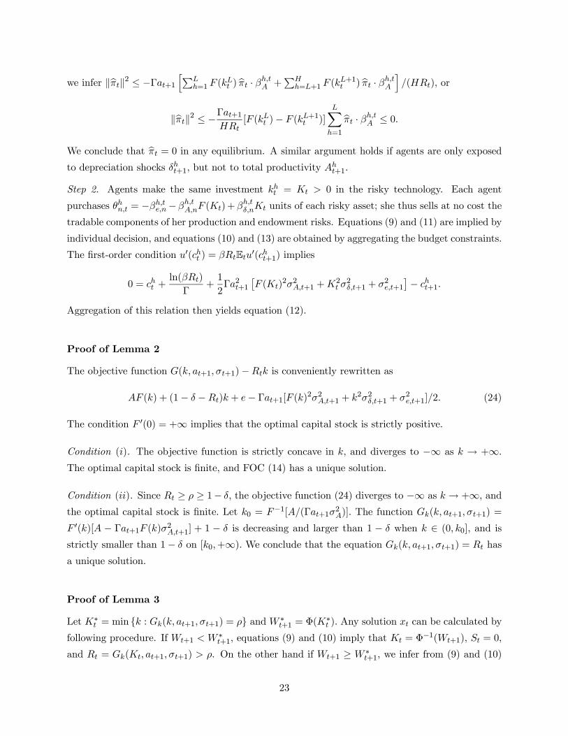
we infer kbπtk2 ≤ −Γat+1 hPLh=1 F (k

Lt ) bπt · βh,tA +

PHh=L+1 F (k

L+1t ) bπt · βh,tA

i/(HRt), or

kbπtk2 ≤ −Γat+1HRt

[F (kLt )− F (kL+1t )]LX

h=1

bπt · βh,tA ≤ 0.

We conclude that bπt = 0 in any equilibrium. A similar argument holds if agents are only exposedto depreciation shocks δht+1, but not to total productivity A

ht+1.

Step 2. Agents make the same investment kht = Kt > 0 in the risky technology. Each agent

purchases θhn,t = −βh,te,n− βh,tA,nF (Kt)+βh,tδ,nKt units of each risky asset; she thus sells at no cost the

tradable components of her production and endowment risks. Equations (9) and (11) are implied by

individual decision, and equations (10) and (13) are obtained by aggregating the budget constraints.

The first-order condition u0(cht ) = βRtEtu0(cht+1) implies

0 = cht +ln(βRt)

Γ+1

2Γa2t+1

£F (Kt)

2σ2A,t+1 +K2t σ

2δ,t+1 + σ2e,t+1

¤− cht+1.

Aggregation of this relation then yields equation (12).

Proof of Lemma 2

The objective function G(k, at+1, σt+1)−Rtk is conveniently rewritten as

AF (k) + (1− δ −Rt)k + e− Γat+1[F (k)2σ2A,t+1 + k2σ2δ,t+1 + σ2e,t+1]/2. (24)

The condition F 0(0) = +∞ implies that the optimal capital stock is strictly positive.

Condition (i). The objective function is strictly concave in k, and diverges to −∞ as k → +∞.

The optimal capital stock is finite, and FOC (14) has a unique solution.

Condition (ii). Since Rt ≥ ρ ≥ 1− δ, the objective function (24) diverges to −∞ as k → +∞, and

the optimal capital stock is finite. Let k0 = F−1[A/(Γat+1σ2A)]. The function Gk(k, at+1, σt+1) =

F 0(k)[A − Γat+1F (k)σ2A,t+1] + 1 − δ is decreasing and larger than 1 − δ when k ∈ (0, k0], and isstrictly smaller than 1− δ on [k0,+∞). We conclude that the equation Gk(k, at+1, σt+1) = Rt has

a unique solution.

Proof of Lemma 3

Let K∗t = min k : Gk(k, at+1, σt+1) = ρ and W ∗

t+1 = Φ(K∗t ). Any solution xt can be calculated by

following procedure. If Wt+1 < W ∗t+1, equations (9) and (10) imply that Kt = Φ

−1(Wt+1), St = 0,

and Rt = Gk(Kt, at+1, σt+1) > ρ. On the other hand if Wt+1 ≥ W ∗t+1, we infer from (9) and (10)

23

that Rt = ρ, Kt = K∗t , and St = [Wt+1−Φ(Kt)]/ρ. Equations (11)− (13) then assign unique values

to at, Ct and Wt. Finally, we observe that (at,Kt, St, Rt) ∈ (0, 1)× R∗+ × R+ × [ρ,+∞), while nosimple restrictions seem to be imposed on current consumption and wealth.

Proof of Proposition 2

Consider a ∈ R and the mapping

ϕ(WT ) =

(W0(WT ) if W0(WT ) is defined and larger than a,

a otherwise.

Since ϕ is continuous on its domain [e,+∞), its image is an interval of the real line. WhenWT → e,

productive investment KT−1 and ST−1 decline to zero, implying that RT−1 → +∞, aT−1 → 1,

CT−1 → −∞, WT−1 → −∞, and ϕ(e) = a. On the other hand when WT → +∞, we observe that

Rt = ρ for all t and ϕ(WT )→ +∞. This establishes that ϕ[e,+∞) = [a,+∞). Since the argumentapplies to any choice of a, we conclude that ϕ(WT ) =W0 has a solution for any W0 ∈ R.

Proof of Proposition 3

Consider an economy with only undiversifiable endowment shocks (σe ≥ 0 and σA = σδ = 0). We

establish the strict monotonicity of W0(·) and thus equilibrium uniqueness by recursively showing

the following

Property. The wealth function Wt(WT ) is strictly increasing in WT . Mean consumption Ct(WT ),

productive investment Kt(KT ) and storage St(ST ) are weakly increasing in WT , while marginal

propensity at(WT ) and the interest rate Rt(WT ) are weakly decreasing.

The statement is true for t = T. Assume that it is true for period t. In the absence of storage, the

capital stock Kt−1 = Φ−1(Wt) locally increases with future wealth Wt and thus terminal wealth

WT ; the interest rate Rt−1 = Φ0(Kt−1) is decreasing in Kt−1 and thus in WT . In the presence of

storage, the safe investment St−1 locally increases in Wt while Rt−1 and Kt−1 are locally constant.

In either case, Kt−1 + St−1 strictly increases with WT . Since at and Rt−1 are both decreasing in

WT , we infer that at−1 = 1/[1 + (atRt−1)−1] is decreasing as well. Consumption

Ct−1 = Ct − ln(βRt−1)/Γ− Γa2tσ2e/2

is therefore increasing in WT . We conclude that Wt−1 = Ct−1+Kt−1+St−1 strictly increases with

the terminal wealth level WT .

24

Proof of Lemma 4

We begin by checking the convergence of the series (17) defining bht . By Assumption [2], the se-

quences at∞t=0 and Rt∞t=0 are contained in compact intervals of the form [a, 1] and [R,R], wherea > 0 and R > 0. It follows that the sequences kht ∞t=0 and Mh

t ∞t=0 are bounded. The determin-istic sequence bht ∞t=0 is thus well-defined and bounded.

We easily check that the consumption-investment plan defined by (7) satisfies the Euler equation

u0(ct) = βRtEtu0(ct+1). Since u0 = −Γu, we infer that u(ct) = βRtEtu(ct+1). The candidate planthus generates utility Jh(W, 0) ≡ E0

P∞t=0 β

tu(ct) = (1 + Π0)u(c0), or equivalently Jh(W, 0) ≡−(Γa0)−1 exp

£−Γ(a0W + bh0)

¤.

We must now verify that Jh(W, 0) is indeed the value function. For a given W , consider

an admissible plan c0t, k0t, s0t, θ0t,W 0t∞t=0 that satisfies W 0

0 = W and the transversality condition

limT→∞ βTE0u(W 0T ) = 0. We know that

Jh(W, 0) = Maxc,k,s,θ,W

hu(c) + βEJh(W1, 1)

i≥ u(c00) + βE0Jh(W 0

1, 1),

and by repetition

Jh(W, 0) ≥ E0

"T−1Xt=0

βtu(c0t)

#+ βTE0Jh(W 0

T , T ). (25)

Since exp(−ΓbhT )/aT∞T=0 is bounded and exp(−ΓaTW 0T ) ≤ 1 + exp(−ΓW 0

T ), the transversality

condition implies that βTE0Jh(W 0T , T ) = −(ΓaT )−1βTE0 exp

£−Γ(aTW 0

T + bhT )¤converges to 0 as

T →∞. We thus obtain that

Jh(W, 0) ≥ E0

"+∞Xt=0

βtu(c0t)

#(26)

for any admissible strategy, and conclude that Jh(W, 0) is the value function.

Proof of Proposition 6

Letting ϕ(R) ≡ Γ−2 (1− 1/R)−2 ln( 1Rβ ), we rewrite system (18)− (19) as:

ϕ(R) =£F (K)2σ2A +K2σ2δ + σ2e

¤/2 (27)

F 0(K)

∙A− Γσ2A

µ1− 1

R

¶F (K)

¸− Γ

µ1− 1

R

¶Kσ2δ + 1− δ −R = 0. (28)

The function ϕ(R) decreases on (1, 1/β] and satisfies ϕ(1, 1/β] = [0,+∞). Equation (27) thus definesthe decreasing function R1(K), which maps [0,+∞) onto (1, ϕ−1(σ2E/2)]. Similarly, equation (28)implicitly defines the decreasing function R2(K) that maps (0,K∗] onto [1,+∞), where K∗ =

(F 0)−1(δ/A).

25

Consider the function ∆(K) = R1(K) − R2(K). When K → 0, we observe that R1(K) →ϕ−1(σ2E/2), R2(K)→ +∞, and therefore ∆(K)→ −∞.We also note that ∆(K∗) = R1(K

∗)− 1 >0. The graphs of the functions R1 and R2 therefore intersect and there exists at least one steady

state.

Finally, we analyze the monotonicity of the steady state with respect to the economy’s parame-

ters. We consider the case |R02(K∞)| > |R01(K∞)|. An increase in σe or β pushes down the functionR1(K) and leaves the function R2(K) unchanged. The steady state is therefore characterized by

a lower interest rate and a higher capital stock. Similarly, an increase in 1 − δ and A pushes up

R2(K), also leading to a lower interest rate and a higher capital stock. We note that an increase

in Γ, σA or σδ pushes down both R1(K) and R2(K) and can have ambiguous effects, as is verified

in simulations.

Proof of Proposition 7

It is enough to provide an example of multiplicity. We numerically check that there exist three

equilibria when Γ = 1.2, A = 20, α = 0.95, β = 0.05, δ = 0.5, σA = 9, σδ = 0, σe = 0, e = 0.

Local Dynamics around the Steady State

There is no storage around the steady state. For computational simplicity, we focus on economies

without undiversifiable depreciation risk. The iterated function H is then implicitly defined by:

Kt = Φ−1(Wt+1),

Rt = F 0(Kt)£A− Γat+1F (Kt)σ

2A

¤+ 1− δ,

at = 1/[1 + (at+1Rt)−1],

Ct = Ct+1 − ln(βRt)/Γ− Γa2t+1£F (Kt)

2σ2A + σ2e¤/2,

Wt = Ct +Kt.

The function H has Jacobian matrix

∂H =

⎡⎢⎢⎣∂at∂at+1

0 ∂at∂Wt+1

∂Ct∂at+1

1 ∂Ct∂Wt+1

∂Ct∂at+1

1 ∂(Ct+Kt)∂Wt+1

⎤⎥⎥⎦ .We observe that ∂Kt/∂Wt+1 = 1/Φ

0(Kt) > 0, and18

∂Rt

∂at+1= −ΓF (Kt)F

0(Kt)σ2A ≤ 0,

∂Rt

∂Wt+1=

1

Φ0(Kt)

©F 00(Kt)

£A− Γat+1F (Kt)σ

2A

¤− at+1[F

0(Kt)]2Γσ2A

ª< 0.

18Since R∞ > 1, we infer that A− Γat+1F (Kt)σ2A > 0 on a neighborhood of the steady state.

26

Let ϕ(v) = 1/(1+v−1).We note that ϕ(v) = v/(1+v) and therefore ϕ0(v) = 1/(1+v)2 = [ϕ(v)/v]2.

Since at = ϕ(at+1Rt), we infer that

∂at∂at+1

=

µat

at+1Rt

¶2µRt − at+1

¯∂Rt

∂at+1

¯¶,

∂at∂Wt+1

= −µ

atat+1Rt

¶2at+1

¯∂Rt

∂Wt+1

¯< 0.

Future propensity at+1 has an ambiguous effect on current propensity at. There is both a positive

direct effect (due to the complementarity of future and current consumption) and a negative indirect

effect (the precautionary motive causes a decline in the current interest rate Rt). Since Ct =

Ct+1 − ln(βRt)/Γ− Γa2t+1£F (Kt)

2σ2A + σ2e¤/2, we infer that

∂Ct

∂at+1=

1

ΓRt

¯∂Rt

∂at+1

¯− Γat+1[F (Kt)

2σ2A + σ2e]

∂Ct

∂Wt+1=

1

ΓRt

¯∂Rt

∂Wt+1

¯− Γa2t+1σ2A

F (Kt)F0(Kt)

Φ0(Kt)

An increase in at+1 and Wt+1 leads to a decline in the current interest rate, which has a positive

effect on current consumption. On the other hand, the increase in at+1 and Wt+1 implies that the

agent bears more risk between time t and time t+ 1. The precautionary motive can then lead to a

decrease in current consumption and current wealth, which may generate endogenous fluctuations.

The characteristic polynomial P (x) = det(∂H − xI) can be rewritten as

P (x) =

µ∂at∂at+1

− x

¶½x2 −

∙1 +

∂(Ct +Kt)

∂Wt+1

¸x+

∂Kt

∂Wt+1

¾+ x

∂Ct

∂at+1

∂at∂Wt+1

.

The roots of P are the eigenvalues of the backward dynamical system. Since P (−∞) = +∞ and

P (+∞) = −∞, there always exists a real eigenvalue. Simple calculation shows that P (1) > 0 if

and only if |R02(K∞)| > |R01(K∞)| . Thus when there is a unique steady state, the Jacobian matrix∂H has an eigenvalue in (1,+∞), and the dimension of the stable manifold is at least 1.

A. Complete Markets

We know that∂at∂at+1

= β,∂Ct

∂at+1= 0,

∂Ct

∂Wt+1> 0,

and the characteristic polynomial is of the form P (x) = (β − x)Q(x), where

Q(x) = x2 −∙1 +

∂(Ct +Kt)

∂Wt+1

¸x+

∂Kt

∂Wt+1.

This implies that x = β is an eigenvalue, which is contained in the interval (0, 1). We observe that

Q(0) > 0 and Q(1) < 0, and infer the polynomial Q has one root in the interval (0, 1) and one root

27

in (1,+∞). Overall, the Jacobian matrix ∂H has two eigenvalues in the interval (0, 1), and one

eigenvalue larger than 1. The stable manifold has thus dimension 1.

B. Endowment Risk - No Productivity Shocks (σe > 0, σA = σδ = 0)

The unique steady state is defined by

ln(R∞β) = −Γ2(1−R−1∞ )2σ2e/2, (29)

R∞ = Φ0(K∞). (30)

The characteristic polynomial simplifies to

P (x) =

µ1

R∞− x

¶½x2 −

∙1 +

1

R∞+

A|F 00(K∞)|ΓR2∞

¸x+

1

R∞

¾+ xΓa2∞R3∞

A¯F 00(K∞)

¯σ2e.

We note that P (1) > 0 and infer that the polynomial has at least one root x1 in (1,+∞). It remainsto characterize the other roots x2 and x3. It is useful to observe that P (0) = R−2∞ ∈ (0, 1).

If the roots x2 and x3 are complex, we know that x3 = x2. The relation P (0) = x1|x2|2 < 1

implies that |x2| < 1. The economy is then stable and locally determined.If the roots x2 and x3 are real, the inequalities x1 > 1 and x1x2x3 = P (0) > 0 implies that

x2 and x3 have the same sign. Furthermore since P (0) < 1, one of these roots is contained in the

interval (−1, 1). We assume without loss of generality that x2 ∈ (−1, 1). We can then consider twocases:

• If x2 and x3 are both positive, the inequalities P (0) > 0 and P (1) > 0 imposes that x2, x3 ∈(0, 1). The steady state is stable and locally determined.

• If on the other hand x2 and x3 are both negative, we know that x3 > −1 if and only ifP (−1) > 0. Since ln(R∞β) = −Γ2(1−R−1∞ )

2σ2e/2 at the steady state, we easily infer

P (−1) = 2µ1

R∞+ 1

¶2+

A|F 00(K∞)|ΓR2∞

∙1 +

1

R∞+ 2

ln(R∞β)

R∞

¸.

The condition R∞ ∈ (1, β−1] implies that

P (−1) ≥ 2µ1 +

1

R∞

¶2+2A|F 00(K∞)|ΓR2∞

(1 + lnβ).

Let β∗ = 1/e ≈ 0.368. Any economy with β ≥ β∗ has a locally determined steady state.

When agents only face uninsurable endowment shocks, it is thus impossible to obtain local

indeterminacy and flip bifurcations with patient agents (i.e. with β ≥ β∗).

Conversely, we can easily show that indeterminacy can arise in economies with sufficient im-

patience and large uninsurable shocks. When σe → +∞, the steady state satisfies R∞ → 1,

28

K∞ → (F 0)−1(δ/A) and Γ2a2∞σ2e → 2 ln(1/β). The characteristic polynomial is then

P (−1) ∼ 2∙4 +

A|F 00(K∞)|Γ

(1− ln 1β)

¸.

We infer that P (−1) < 0 for a sufficiently low value of β. This result is consistent with the

indeterminacy obtained in Calvet (2001) for exchange economies with sufficient impatience and

large uninsurable endowment shocks.

C. Uninsurable Productivity Shocks

Consider the parameter values: β = 0.95, Γ = 2, A = 10, α = 0.35, δ = 0.1, σδ = 0, σe = 0.

We check numerically that the steady state is unique and that the characteristic polynomial has

one eigenvalue x1 > 1 and two eigenvalues in the unit circle when σA ≤ 30.5. On the other handwhen σA = 31.5, the steady state remains unique but there is one eigenvalue in each of the interval

(−∞,−1), (−1, 1) and (1,+∞). This establishes Proposition 8. We also note that the systemundergoes a flip bifurcation as σA varies between 30.5 and 31.5, which proves Proposition 9.

Finally, consider the economy Γ = 1.2, A = 20, α = 0.95, β = 0.05, δ = 0.5, σA = 9, σe = 0,

σδ = 0, e = 0 examined in the proof of Proposition 7. This economy has three steady states, and

it can be checked numerically that the steady state with the intermediate interest rate is totally

unstable, thus establishing Proposition 10.

Proof of Proposition 11

We know thatGk(Kt,Xt) = Rt, we infer that Fx (Kt,Xt) [1−Γat+1σ2AF (Kt,Xt)] = Rt+Γat+1σ2xXt,

which implies

1− Γat+1σ2AF (Kt,Xt) > 0.

Equation (20) can be rewritten as

Kαt X

ηt

µη

Xt− α

Kt

¶= (σ2xXt − σ2kKt)

Γat+11− Γat+1σ2AF (Kt,Xt)

. (31)

We consider parameters satisfying σk/σx <pη/α, and assume that Xt/Kt ≥ η/α. The left-hand

side of (31) is weakly negative. On the other hand since Xt/Kt ≥ η/α > σ2k/σ2x, the right-hand

side of (31) is strictly positive - a contradiction. We conclude that Xt/Kt < η/α.

Proof of Proposition 12

The proposition is a direct application of Sard’s theorem. We assume for notational simplicity that

there are two sectors (J = 2). For a given sequence Rt∞t=0, consider the function

H(k1, k2;σ1, σ2) =

∙∂G1∂k

(k1, σ1)−Rt;∂G2∂k

(k2, σ2)−Rt;F01(k1)− F 02(k2)

¸.

29

It is easy to check that the Jacobian matrix of H has rank 3 whenever H(k1, k2;σ1, σ2) = 0. We

conclude that the system H = 0 has no solution for almost every choice of (σ1, σ2).

References

Aghion, P., Bacchetta, P., Banerjee, A., 2000. “Capital Markets and the Instability of Open Economies,”

manuscript, Harvard University.

Aghion, P., Banerjee, A., Piketty, T., 1999. Dualism and Macroeconomic Activity. Quarterly Journal of

Economics 114, 1359-1397.

Aiyagari, S. R., 1994. Uninsured Idiosyncratic Risk and Aggregate Saving. Quarterly Journal of Economics

109, 659-684.

Angeletos, G. M., Calvet, L. E., 2003. “Idiosyncratic Production Risk, Growth and the Business Cycle.”

NBER Working Paper 9764. Forthcoming in Journal of Monetary Economics.

Banerjee, A., and Newman, A., 1991. Risk-Bearing and the Theory of Income Distribution. Review of

Economic Studies 58, 211-235.

Benhabib, J., Day, R., 1982. A Characterization of Erratic Dynamics in the Overlapping Generations Model.

Journal of Economic Dynamics and Control 4, 37-55.

Benhabib, J., Farmer, R., 1994. Indeterminacy and Increasing Returns. Journal of Economic Theory 63,

19-41.

Benhabib, J., Nishimura, K., 1979. The Hopf Bifurcation and the Existence and Stability of Closed Orbits

in Multisector Models of Optimal Economic Growth. Journal of Economic Theory 21, 421-444.

Boldrin, M., Montrucchio, L., 1986. On the Indeterminacy of Capital Accumulation Paths. Journal of

Economic Theory 40, 26-39.

Brock, W., Mirman, L., 1972. Optimal Economic Growth and Uncertainty: The Discounted Case. Journal

of Economic Theory 4, 497-513.

Caballero, R., 1990. Consumption Puzzles and Precautionary Saving. Journal of Monetary Economics 25,

113-136.

Calvet, L. E., 2001. Incomplete Markets and Volatility. Journal of Economic Theory 98, 295-338.

Cass, D., 1965. Optimum Growth in an Aggregative Model of Capital Accumulation. Review of Economic

Studies 32, 233-240.

30

Constantinides, G., Duffie, D., 1996. Asset Pricing with Heterogeneous Consumers. Journal of Political

Economy 104, 219-240.

Deneckere, R., Pelikan, S., 1986. Competitive Chaos. Journal of Economic Theory 40, 13-25.

Galor, O., Zeira, J., 1993. Income Distribution and Macroeconomics. Review of Economic Studies 60, 35-52.

Grandmont, J. M., 1985. On Endogenous Competitive Business Cycles. Econometrica 53, 995-1045.

Heaton, J., Lucas, D. J., 1996. Evaluating the Effects of Incomplete Markets on Risk Sharing and Asset

Pricing. Journal of Political Economy 104, 443-487.

Huggett, M., 1997. The One-Sector Growth Model with Idiosyncratic Shocks: Steady States and Dynamics.

Journal of Monetary Economics 39, 385-403.

Kiyotaki, N., Moore, J., 1997. Credit Cycles. Journal of Political Economy 105, 211-248.

Koopmans, T. C., 1965. On the Concept of Optimal Economic Growth, in: The Economic Approach to

Development Planning (North-Holland, Amsterdam).

Krebs, T., 2003. Human Capital Risk and Economic Growth. Quarterly Journal of Economics 118, 709-744.

Krusell, P., Smith, A., 1998. Income and Wealth Heterogeneity in the Macroeconomy. Journal of Political

Economy 106, 867-896.

Leland, H., 1968. Saving and Uncertainty: The Precautionary Demand for Saving. Quarterly Journal of

Economics 82, 465-473.

Ljungqvist, L., Sargent, T. J., 2000. Recursive Macroeconomic Theory. MIT Press.

Mankiw, N. G., 1986. The Equity Premium and the Concentration of Aggregate Shocks. Journal of Financial

Economics 17, 211-219.

Marcet, A., Obiols-Hom, F., Weil, P., 2000. Incomplete Markets, Labor Supply and Capital Accumulation.

Working Paper, Universitat Pompeu-Fabra.

Mitra, T., 1996. An Exact Discount Factor Restriction for Period-Three Cycles in Dynamic Optimization

Models. Journal of Economic Theory 69, 281-305.

Nishimura, K., Yano, M., 1996. On the Least Upper Bound of Discount Factors That Are Compatible with

Optimal Period-Three Cycles. Journal of Economic Theory 69, 306-333.

Sandmo, A., 1970. The Effect of Uncertainty on Saving Decisions. Review of Economic Studies 37, 353-360.

Sorger, G., 1992. On the Minimum Rate of Impatience for Complicated Optimal Growth Paths. Journal of

Economic Theory 56, 160-179.

Weil, P., 1992. Equilibrium Asset Prices in Economies with Undiversifiable Labor Income Risk. Journal of

Economic Dynamics and Control 16, 769-790.

31

Figure 1A. Finite-Horizon Growth Path

We plot the time paths of wealth, interest rate, capital, storage, consumption and

marginal propensity to consume for a finite-horizon economy (T = 1000) with

uninsurable idiosyncratic production risk (σA > 0).

250 500 750 1000t

10

15

20

Wealth Wt

250 500 750 1000t

0.96

0.98

1.02

1.04

1.06Interest Rate Rt

250 500 750 1000t

5

10

15

20

Capital Kt

250 500 750 1000t

2

4

6

8

10Storage St

250 500 750 1000t

1.75

2

2.25

Consumption Ct

250 500 750 1000t

0.018

0.022

0.024

M.P.C. at

Figure 1B. Turnpike Property

The figure plots ln(Wt/ W ), which quantifies the distance between the wealth W

tin

period t of a finite-horizon economy (T = 1000) and the steady-state level of wealth

W under infinite horizon (T = ). The economy is the same as in Figure 1A.

200 400 600 800 1000t

-0.4

-0.3

-0.2

-0.1

0.1

0.2

0.3

ln Wt W

Figure 2. Nonmonotonicity of W0(WT)

10 20 30 40 50 60 70WT

1

2

3

4

5

W0

Multiple equilibria in a finite-horizon economy with idiosyncratic production risk and

patient agents (β = 0.9). The figure illustrates the non-monotonic relation between

initial and final wealth. For any given W0 [1,3], there are multiple WT

corresponding

to different equilibrium paths.

Figure 3. Endogenous Fluctuations in Finite Horizon

We plot the time paths of aggregate wealth, interest rate, capital investment, storage,

consumption, and marginal propensity to consume in a finite-horizon economy with

idiosyncratic production risk and patient agents (β = 0.99).

10 20 30 40 50t

5

10

Wealth Wt

10 20 30 40 50t

5

10

Interest Rate Rt

10 20 30 40 50t

0.2

0.4

0.6

0.8

Capital Kt

10 20 30 40 50t

2

4

6

8Storage St

10 20 30 40 50t

1

2

3

4Consumption Ct

10 20 30 40 50t

0.02

0.04

0.06

0.08

M.P.C. at