IEEE TRANSACTIONS ON COMMUNICATIONS, VOL. XX, NO. Y, MONTH 2007 1

Cross-layer Adaptive Transmission with Incomplete

System State InformationAnh Tuan Hoang, Member, IEEE, and Mehul Motani, Member, IEEE

Abstract— We consider a point-to-point communication systemin which data packets randomly arrive to a finite-length bufferand are subsequently transmitted to a receiver over a time-varying wireless channel. Data packets are subject to loss due tobuffer overflow and transmission errors. We study the problemof adapting the transmit power and rate based on the buffer andchannel conditions so that the system throughput is maximized,subject to an average transmit power constraint. Here, the systemthroughput is defined as the rate at which packets are successfullytransmitted to the receiver. We consider this buffer/channel adap-tive transmission when only incomplete system state informationis available for making control decisions. Incomplete systemstate information includes delayed and/or imperfectly estimatedchannel gain and quantized buffer occupancy. We show that,when some delayed but error-free channel state information isavailable, optimal buffer/channel adaptive transmission policiescan be obtained using Markov decision theories. When thechannel state information is subject to errors and when thebuffer occupancy is quantized, we discuss various buffer/channeladaptive heuristics that achieve good performance. In this paper,we also consider the tradeoff between packet loss due to bufferoverflow and packet loss due to transmission errors. We showby simulation that exploiting this tradeoff leads to a significantgain in the system throughput.

Index Terms— Cross-layer design, adaptive transmission,

throughput maximization, partially observable Markov decision

processes.

I. INTRODUCTION

In this paper, we study the problem of buffer and channel

adaptive transmission in a point-to-point wireless communi-

cation scenario with the objective of maximizing the system

throughput, subject to an average transmit power constraint.

We term our adaptive transmission schemes cross-layer since

transmission decisions at the physical layer take into account

not only the channel condition but also the data arrival

statistics and buffer occupancy, which are the parameters of

higher network layers.

Our system model is depicted in Fig. 1. Time is divided

into frames of equal length and during each frame, data

packets arrive at the transmitter buffer according to some

known stochastic distribution. The buffer has a finite length

and when there is no space left, arriving packets are dropped.

Manuscript received November 08, 2006; revised May 31, 2007, andAugust 22, 2007.

A. T. Hoang is with the Department of Networking Protocols, Institute forInfocomm Research (I2R), 21 Heng Mui Keng Terrace, Singapore 119613.Previously, he was with the Department of Electrical and Computer Engineer-ing, National University of Singapore. E-mail: athoang@i2r.a-star.edu.sg.

M. Motani is with the Department of Electrical and Computer En-gineering, National University of Singapore, Singapore 119260. E-mail:motani@nus.edu.sg.

Data packets in the buffer are transmitted to a receiver over

a discrete-time block-fading channel. The fading process is

represented by a finite state Markov chain (FSMC) ( [1], [2]).

We define the system state during each time frame as the

combination of the buffer occupancy and the channel state and

assume that there is a signaling mechanism for the transmitter

and receiver to exchange some system state information (SSI).

In our system model, data packets are subject to loss due

to buffer overflow and transmission errors. We define the

system throughput as the rate at which packets are successfully

transmitted to the receiver. The control problem is to adapt

the transmit power and rate according to some SSI so that the

system throughput is maximized, subject to an average trans-

mit power constraint. We are interested in scenarios in which

only an incomplete observation of the instantaneous system

state is available for making control decisions. Incomplete

SSI includes delayed and/or imperfectly estimated channel

state and quantized buffer occupancy. The case when control

decisions can be made based on complete SSI is considered

in our related work [3], where interesting structural properties

of optimal adaptive transmission policies are studied.

In the context of adaptive transmission, our paper is related

to the well-known works of Goldsmith in [4] and [5]. In these

works, it is shown that when the channel state information

(CSI) is available at both the transmitter and receiver, the

optimal power allocation scheme that achieves the capacity of

a time-varying wireless channel, subject to an average transmit

power constraint, exhibits a water-filling structure over time.

The insight is that the transmitter should transmit at a higher

power and rate when the channel is good while reducing the

transmit power in poorer channel conditions. However, data

arrival statistics and buffer conditions are not of concern in

[4] and [5].

In the context of cross-layer design, our paper is closely

related to the works in [6]–[16], which consider similar

problems of buffer/channel adaptive transmission. An early

work of Collins and Cruz adapts transmit power and rate

based on the queue length and channel condition in order to

minimize the average transmit power, subject to an average

delay constraint [6]. In [7] Berry and Gallager quantify the

behavior of the power-delay tradeoff in the regime of asymp-

totically large delay. The same model is further studied in [8],

[9], with some structural properties of the optimal policies

identified. In [10], Rajan et al. consider a more generalized

queueing model where packets can be dropped. They propose

transmission policies that are near-optimal, in terms of mini-

mizing packet loss subject to an average delay and an average

power constraint. In [11], Karmokar et al. further extend the

IEEE TRANSACTIONS ON COMMUNICATIONS, VOL. XX, NO. Y, MONTH 2007 2

Transmitter Receiver Wireless

Channel

Control Signals Buffer

Packets

Fig. 1. System model of a point-to-point wireless communication scenario.Data packets arrive to the buffer according to some stochastic distribution.The packets are then transmitted over a time-varying wireless channel. Thereare control signals for the transmitter and receiver to exchange buffer andchannel state information.

tradeoff to include average packet delay, average transmit

power, and average packet dropping probability. They also

propose a suboptimal policy that approximates the behaviors

of the optimal policies. In [12]–[16] the problem of cross-layer

adaptive transmission is considered from a different angle

in which transmission is carried out given a fixed amount

of energy and a limited amount of time. The authors adapt

the transmit power and rate according to the amount of data

remaining, the present time relative to the deadline, and the

present channel state, in order to maximize the achievable

throughput ( [12]–[14]) or to maximize the probability of a

data file being successfully transmitted ( [15], [16]).

We note that the works in [6]–[16] assume perfect knowl-

edge of the instantaneous buffer occupancy and channel state.

In [17], Karmokar et al. consider the problem of adapting the

error control coding scheme base on some imperfect observa-

tions of traffic statistics and channel condition. In particular,

the channel observations are in the form of NACK/ACK that

are fed back from the receiver to the transmitter. Similar to

our paper, the problem in [17] is formulated as a partially

observable Markov decision process (POMDP). Even though

the problem setup in [17] differs from that of our paper in

several points, the authors come to a similar conclusion that,

given partial observations, a heuristic called QMDP ( [18])

achieves good performance.

An important contribution that differentiates our work from

[6]–[16] is that we exploit the tradeoff between packet loss

due to buffer overflow and packet loss due to transmission

errors. Our results show that, by balancing these sources of

packet loss, significant gain in the system throughput can

be achieved. From the implementation point of view, when

imperfect channel state information is considered, it is not

possible to calculate transmit power to guarantee a target

packet error rate. We note that the problem formulation in

[10] and [16] allows for optimizing over both packet losses

due to transmission failure and buffer overflow. However, their

assumptions result in no packet losses due to transmission

errors. Specifically, their policies never transmit above the

Shannon capacity and they assume no transmission errors

at rates below capacity. In their recent works ( [19], [20]),

Liu at al. do take into account both packet losses due to

transmission errors and buffer overflows. Their definition of

system throughput is also similar to ours. However, the policies

considered in [19], [20] adapt to the channel state information

only, not to the buffer and data arrival statistics.

The main contributions of this paper can be summarized as

follows.

• We present tractable models of buffer/channel adaptive

transmission given imperfect SSI.

• We exploit the tradeoff between packet loss due to buffer

overflow and packet loss due to transmission errors. This

tradeoff results in a performance gain in the overall

system throughput.

• We show how buffer and channel adaptive transmission

can be carried out given incomplete SSI. In particular, we

show that optimal adaptive policies can be obtained for

the cases when some delayed but error-free channel state

information is available. When the channel state informa-

tion is subject to errors and when the buffer occupancy

is quantized, we present various buffer/channel adaptive

heuristics that achieve good performance.

The rest of this paper is organized as follows. In Section II,

we present our system model and discuss the approach that can

be used to obtain optimal adaptive transmission policies when

the transmit power and rate can be chosen based on a perfect

knowledge of the instantaneous system state. Next, in Section

III, we discuss the situations in which the transmitter and

receiver only have partial information about the current buffer

and channel states. In Section IV, we show that optimal control

policies can be obtained when some delayed but error-free

channel states are available for making decision. When this is

not possible, we propose various heuristics to obtain policies

with good performance in Section V. Numerical results and

discussion are given in Section VI. Finally, we conclude the

paper in Section VII.

II. THROUGHPUT MAXIMIZATION PROBLEM

A. System Model

The system model considered in this paper is depicted in

Fig. 1. Time is divided into frames of equal length of Tf

seconds. During frame i, Ai packets arrive at the transmitter

buffer. We assume that Ai is independent and identically dis-

tributed (i.i.d.) over time and follows a stationary distribution

pA(a). Each data packet contains L bits, the buffer can store

up to B packets and when the buffer is full, all arriving packets

are dropped. We further assume that arriving packets are only

added to the buffer at the end of each time frame.

We consider a discrete-time block-fading channel with

additive white Gaussian noise (AWGN). The fading process

is represented by a stationary and ergodic K-state Markov

chain, with the channel states numbered from 0 to K−1. The

power gain of channel state g, g ∈ {0, . . .K − 1}, is denoted

by γg . During each time frame, we assume that the channel

remains in a single state, between two consecutive frames, the

probability of transitioning from channel state g to channel

state g′ is denoted by PG(g, g′). The stationary distribution of

each channel state is denoted by pG(g).In general, a finite state Markov channel model (FSMC)

is suitable for modeling a slowly varying flat-fading channel

[1], [21]–[23]. A FSMC is constructed for a particular fading

distribution, e.g., log-normal shadowing or Rayleigh fading,

by first partitioning the range of the fading gain into a finite

number of sections. Then each section of the gain value

corresponds to a state in the Markov chain. Given knowledge

of the fading process, the stationary distribution pG(g) as well

IEEE TRANSACTIONS ON COMMUNICATIONS, VOL. XX, NO. Y, MONTH 2007 3

as the channel state transition probabilities PG(g, g′) can be

derived. For more details, the reader is referred to [1], [21]–

[23].

Let Bi denote the number of packets in the buffer at the

beginning of frame i and Gi denote the channel state through-

out frame i, the system state at frame i is Si , (Bi, Gi). For

time frame i, let Pi(Watts) and Ui(packets/frame) denote the

transmit power and rate, respectively. We have 0 ≤ Ui ≤ Bi

and Pi ∈ P , where P is the set of all power levels at which

the transmitter can operate.

B. Buffer and Channel Adaptive Transmission

Given a particular system state (b, g), where b is the buffer

occupancy and g is the channel state (0 ≤ b ≤ B, 0 ≤ g <K), each chosen pair of transmission rate and power (u, P )results in some expected number of packets lost due to buffer

overflow and transmission errors. We characterize these losses

by two functions: Lo(b, u) is the expected number of packets

lost due to buffer overflow and Le(g, u, P ) is the expected

number of packets discarded due to transmission error. Note

that in this paper, we do not consider retransmission of

erroneous packets.

For our system model, when the data arrival process is fixed,

maximizing the system throughput is equivalent to minimizing

total packet loss due to buffer overflow and transmission

errors. This is achieved by varying the transmission rate and

power (Ui, Pi) according to some knowledge of Si. Note

that there are various ways for the transmitter to change its

transmission rate Ui. It can be done by changing the channel

coding scheme [24], i.e. by encoding data bits in the buffer

using different code rates while keeping the transmission rate

for the coded bits fixed. Ui can also be varied by keeping the

symbol rate fixed and changing the signal constellation size of

a modulator [5], [8], [25]. In existing communication standards

such as IEEE.802.11 and IEEE.802.16, different transmission

rates are achieved by combinations of different coding and

modulation schemes.

C. Buffer Overflow and Transmission Error Tradeoff

At this point, let us point out an interesting tradeoff between

the two sources of packet loss, i.e., buffer overflow and

transmission errors. Consider a particular system state (b, g)and a fixed transmit power P . If we increase the transmission

rate u, the amount of buffer overflow is reduced. However,

increasing u when P is fixed results in a greater number of

packet transmission errors. The reverse is also true, for fixed

P , the amount of packet transmission errors can be reduced by

lowering the transmission rate u, but that will be at the cost of

increasing the buffer overflow rate. This argument highlights

the need to find a good tradeoff between packet transmission

errors and buffer overflow when choosing transmit power and

rate. In this paper, our control decision strives for an optimal

tradeoff between these two sources of packet loss.

D. Throughput Maximization with Complete SSI

Before considering buffer/channel adaptive transmission

with incomplete SSI, let us briefly discuss how optimal

buffer/channel adaptive transmission policies can be obtained

for the case of complete SSI. With complete SSI, the through-

put maximization problem can be reformulated as the problem

of minimizing the weighted sum of the long-term packet loss

rate and the average transmission power. In particular, consider

the following problem of selecting transmission rate and power

(Ui, Pi):

arg minUi,Pi

{lim supT→∞

1

TE

{T−1∑

i=0

C(Bi, Gi, Ui, Pi)

}}, (1)

where

C(b, g, u, P ) = P + β (Lo(b, u) + Le(g, u, P )) . (2)

Here β is a positive weighting factor that gives the priority

of reducing packet loss over conserving power. When β is

increased, we tend to transmit at a higher rate in order to lower

the packet loss rate at the expense of using higher transmit

power. On the other hand, for smaller values of β, the average

transmission power will be reduced at the cost of increasing

the packet loss rate. If P β and Lβ are the average power

and packet loss rate (due to buffer overflow and transmission

errors) obtained when solving (1) for a particular value of

β, then Lβ is also the minimum achievable loss rate given a

power constraint of P β .

For our system model in which the channel state Gi

evolves according to a stationary, ergodic Markov process, the

optimization problem in (1) can be classified as an infinite-

horizon, average-cost Markov decision process [26]. For such

a problem, given complete system SSI, there exists a stationary

control policy that is optimal. Let π be a stationary policy

which maps system states into transmission rate and power

for each frame i, i.e., π(Bi, Gi) , (Ui, Pi). Defining

Javr(π) = lim supT→∞

1

TE

{T−1∑

i=0

C(Bi, Gi, Ui, Pi) | π

}, (3)

the optimization problem in (1) becomes

π∗ = arg min

πJavr(π). (4)

The above infinite-horizon, average-cost Markov decision pro-

cess (MDP) can be solved effectively using dynamic program-

ming techniques such as policy iteration and value iteration

[26, Chapter 6].

It is also useful to consider the discounted cost of using

policy π with initial system state (b, g), i.e.,

Jα(b, g, π)

= limT→∞

E

{T−1∑

i=0

αiC (Bi, Gi, Ui, Pi) |B0 = b, G0 = g, π

},

(5)

where 0 < α < 1 is the discounting factor. As the immediate

cost function C(b, g, u, P ) is bounded, the limit in (5) always

exists. Correspondingly, we have the problem of finding a

control policy that minimizes the discounted cost, i.e.,

π∗α = arg min

πJα(b, g, π). (6)

IEEE TRANSACTIONS ON COMMUNICATIONS, VOL. XX, NO. Y, MONTH 2007 4

It can be shown that π∗α converges to π

∗ which is the solution

of (4) as α → 1 ( [26, Chapter 6]). Moreover, let J∗α(b, g) be

the minimum discounted cost when starting with initial state

(b, g), the solution of the discounted cost problem satisfies the

simple Bellman equation ( [26, Chapter 6]):

J∗α(b, g) = min

(u,P )

{C (b, g, u, P ) + α

K−1∑

g′=0

∞∑

a=0

(PG(g, g′)

pA(a)J∗α

(min{b − u + a, B}, g′

))}.

(7)

The physical interpretation of (7) is that, for the discounted

cost problem, at each stage of control, the optimal control

action should minimize the sum of the immediate cost C(.)and the α-weighted future cost, provided that in the sub-

sequent future stages, optimal control actions are selected.

This elegant Bellman equation is useful for analyzing the

structural properties of optimal control policies. It is also

the inspiration behind the effective QMDP heuristic ( [18])

when only incomplete system state information is available

for making control decisions. This is discussed in Section V-

B.3.

III. INCOMPLETE SYSTEM STATE INFORMATION

Let us now consider the cases when only imperfect knowl-

edge of the instantaneous system state is available for making

control decisions. Rather, the transmit power and rate are

adapted based on a partially observed system state which

includes quantized buffer occupancy and delayed and/or im-

perfectly estimated channel state.

A. Quantized Buffer State Information

Although the transmitter usually knows the exact buffer

occupancy, we may not want to adapt the transmission pa-

rameters to this exact value. Firstly, the buffer occupancy can

change frequently, therefore, adapting to its exact value may

require a significant amount of signaling from the transmitter

to the receiver. Secondly, apart from the signaling issue,

we may want to quantize the buffer occupancy in order to

reduce the complexity in obtaining and implementing the

buffer/channel adaptive policies. Given that the buffer capacity

is B and the number of channel states is K , using the exact

buffer occupancy results in the total number of system states of

(B +1)K . When B and K are large, by quantizing B using a

small number of levels, we can significantly reduce the number

of system states and consequently reduce the complexity of

obtaining and implementing the adaptive transmission policies.

We can quantize the buffer occupancy using a small number

of thresholds and only update the transmit power and rate

when there is a threshold crossing. In this paper, the buffer

occupancy is quantized using M +1 thresholds, i.e., 0 = b0 <b1 < . . . < bM = B+1. The buffer is said to be in state k, 0 ≤k < M , if the number of packets currently queueing satisfies

bk ≤ b < bk+1. Denoting the quantized buffer occupancy at

time i by Bi, we have

Bi = bk, where k satisfies bk ≤ Bi < bk+1 . (8)

B. Delayed Imperfect Channel Estimates

We assume that the channel gain is first estimated at

the receiver, then quantized into one of the possible values

{γ0, γ1, . . . γK−1}, and finally the estimated channel index is

fed back to the transmitter. This process introduces both delay

and errors in the transmitter knowledge of the channel state.

If we take into account the effects of both delay and errors,

then at time i, what available at the transmitter is a sequence

of delayed imperfect estimates of the channel states up to time

i−m, i.e., {G0, . . . Gi−m}, i ≥ m ≥ 0. Note that mTf is the

total estimation and feedback delay. We account for the fact

that Gi can be erroneous by the following function:

PE(g, g) = Pr(Gi = g | Gi = g), (9)

which gives the probability of wrongly estimating channel

state g as channel state g. Note that PE(g, g) depends on the

specific channel estimation technique employed at the receiver.

In this paper, we assume that the channel estimation error

does not depend on the chosen transmission parameters and

is i.i.d. over time. We also assume that PE(g, g) is known at

the transmitter for all pairs (g, g).As an example, let us assume that if the actual channel state

is g, then the estimated channel gain prior to quantization is

of the form:

γ = γg + v, (10)

where v is a Gaussian random variable with zero mean and

variance σ2. Quantizing γ to the closest value in the set

{γ0, γ1, . . . γK−1} to obtain the estimated channel index g,

we have:

PE(g, g) =1

2

(erf(γbg + γbg+1 − 2γg

2√

2σ

)

− erf(γbg + γbg−1 − 2γg

2√

2σ

)), 0 < g < K − 1,

(11)

and

PE(g, 0) =1

2

(1 + erf

(γ0 + γ1 − 2γg

2√

2σ

)), (12)

PE(g, K − 1) =1

2

(1 − erf

(γK−2 + γK−1 − 2γg

2√

2σ

)),

(13)

where erf(.) is the standard error function.

IV. OPTIMAL ADAPTIVE TRANSMISSION POLICIES GIVEN

DELAYED ERROR-FREE CHANNEL STATES

In this section, we consider a special case in which

the channel information for choosing the transmit

power and rate at time frame i is of the form

{G0, . . .Gi−m−n, Gi−m−n+1, . . . Gi−m}, i ≥ m + n, m ≥0, n ≥ 0. This means that, at time i, in addition to the

imperfect channel estimates {Gi−m−n+1, . . . Gi−m}, the

transmitter knows all the exact channel states up to time

i − m − n. This assumption can be justified by the fact

that the accuracy of channel estimation process may be

improved if the receiver is given extra time and information

to do processing [5]. For example, when a certain estimation

delay is permitted, the receiver can interpolate between past

IEEE TRANSACTIONS ON COMMUNICATIONS, VOL. XX, NO. Y, MONTH 2007 5

and future estimates to obtain more accurate predictions.

Therefore, our assumption corresponds to the case when the

delay (m + n)Tf is long enough so that the receiver can

obtain a near perfect channel estimate.

Due to the Markov property of the channel model, it is

enough to only maintain a truncated sequence of the channel

observation history which can be represented by the following

channel observation vector:

Hi = (Gi−m−n, Gi−m−n+1 . . . Gi−m). (14)

As there are K possible channel states, the number of all pos-

sible channel observation vectors Hi is Kn+1. The important

point to note is that even though the channel state information

is incomplete, the number of possible values for Hi is still

finite. This allows the problem of minimizing a weighted

sum of the long term packet loss rate and average transmit

power to be formulated as a finite-state MDP, with the actual

channel state Gi being replaced by the channel observation

vector Hi. In order to fully specify the MDP, we need to

derive the dynamics of Hi, together with the cost functions

associated with choosing transmission rate and power (u, P )in state (Bi, Hi).

A. When Hi = (Gi−1, Gi)

To simplify the derivations, we consider the case when

Hi = (Gi−1, Gi). Physically, this means that at time i,the transmitter knows the exact previous channel state Gi−1

and has an estimate of the current channel state Gi. This

corresponds to setting m = 0 and n = 1 in (14). We note

that the subsequent derivations can be extended for general

values of m and n.

At time i, given the channel observation vector H i =(Gi−1, Gi), we can derive the conditional probability distri-

bution of the channel state Gi as:

ρG

(g, g, g

), Pr(Gi = g|Hi = (g, g))

= Pr(Gi = g|Gi−1 = g, Gi = g)

=Pr(Gi = g, Gi−1 = g, Gi = g)

Pr(Gi−1 = g, Gi = g)

=Pr(Gi = g, Gi = g|Gi−1 = g)Pr(Gi−1 = g)

Pr(Gi = g|Gi−1 = g)Pr(Gi−1 = g)

=Pr(Gi = g, Gi = g|Gi−1 = g)

Pr(Gi = g|Gi−1 = g)

=PG(g, g)PE(g, g)

∑K−1g′=0 PG(g, g′)PE(g′, g)

.

(15)

Based on (15), the dynamics of H i can be written as:

PH(g, g, g′, g′) , Pr(H i+1 = (g′, g′)|H i = (g, g)

)

= Pr(Gi = g′, Gi+1 = g′ |H i = (g, g)

)

= Pr(Gi = g′|Hi = (g, g)

)Pr(Gi+1 = g′|Gi = g′)

= ρG(g′, g, g) ×K−1∑

k=0

PG(g′, k)PE(k, g′).

(16)

At time i, given that the buffer occupancy is Bi = b and the

channel observation vector is H i = (g, g), if the transmission

rate and power are set to u and P respectively, the average

number of packets lost due to buffer overflow is still given

by Lo(b, u) while the expected number of packets lost due to

transmission error is

LHe (g, g, u, P ) =

K−1∑

g=0

ρG

(g, g, g

)Le(g, u, P ). (17)

Knowing the dynamics of H i together with the cost of a

transmission action in each state (Bi, Hi), an MDP can be

readily formulated, i.e., similar to that given in Section II-D,

to minimize the weighted sum of the long term packet loss

rate and average transmit power.

B. When Hi = Gi−m

In the special case when Hi = Gi−m, i.e., the transmission

decisions at time i can be made based on the perfect knowl-

edge of channel state at time i − m, the number of possible

values for H i is K . As the result, the size of the newly form

MDP is the same as the size of the MDP for the case of

complete channel state information.

V. ADAPTIVE TRANSMISSION POLICIES WHEN NO

ERROR-FREE CHANNEL STATE IS AVAILABLE

Now, we consider the situation when no delayed error-free

channel estimate is available for choosing transmit power and

rate. At time i, the transmitter knows a sequence of imperfect

channel estimates which can be represented by the following

channel observation vector:

Ii = (G0 . . . Gi−m). (18)

A. Optimal Control Policy Given Delayed Imperfect Channel

Estimates With i.i.d. Channel Model

In the special case when the channel states are i.i.d. over

time, there is no extra information gained by keeping estimates

of past channel states. We suppose that during frame i, the

transmitter knows the estimates of channel state i, i.e., Gi,

then the channel observation vector Ii in (18) is simplified to

defined as

Ii = Gi. (19)

The dynamics of Ii can be derived as:

PI(g, g′) , Pr(Ii+1 = g′|Ii = g)

= Pr(Gi+1 = g′|Gi = g) =K−1∑

g=0

PE(g, g′)pG(g).(20)

Also, during time frame i, given that the channel estimate

is Ii = g, we can derive the probability distribution of the

current channel states as

φG(g, g) , Pr(Gi = g|Ii = g) = Pr(Gi = g|Gi = g)

=PE(g, g)pG(g)

∑K−1g′=0 PE(g′, g)pG(g′)

.(21)

IEEE TRANSACTIONS ON COMMUNICATIONS, VOL. XX, NO. Y, MONTH 2007 6

At time i, given that the buffer occupancy is Bi = b and

the channel observation vector is Ii = (g), if the transmission

rate and power are set to u and P respectively, the average

number of packets lost due to buffer overflow is still given

by Lo(b, u) while the expected number of packets lost due to

transmission error is

LIe(g, u, P ) =

K−1∑

g=0

φG

(g, g)Le(g, u, P ). (22)

Note that the number of possible values for Ii is K .

Knowing the dynamics of Ii together with the cost of a

transmission action in each state (Bi, Ii), an MDP can be

readily formulated, i.e., similar to that given in Section II-D,

to minimize the weighted sum of the long term packet loss

rate and average transmit power.

B. Suboptimal Control Policies Given Imperfect Channel Es-

timates

Now let us consider the case when the channel states are

correlated over time and at time i, the transmitter knows

only a sequence of delayed imperfect channel estimates Ii =(G0 . . . Gi−m). To simplify the notations, we further assume

that m = 0, however, when m > 0 the analysis is similar.

The control problem in this situation can be modeled as a

partially observable Markov decision process (POMDP). For a

POMDP in which the system states are correlated over time, in

order to make an optimal control decision, the controller needs

to keep track of the entire observation history. That means

for our control problem, the transmitter needs to record the

entire channel estimation history, i.e., Ii, in order to select

optimal transmit power and rate. Instead of remembering the

entire observation history, the controller in a POMDP can keep

track of the so called belief state, which is the probability

distribution of the system state, conditioned on the observation

history. For our particular problem, we can define Ψi as the

belief channel state at time i, i.e., then

Ψi(g) = Pr(Gi = g | Ψ0, G0, . . . Gi), (23)

where the initial probability distribution Ψ0 is assumed

known. In case Ψ0 is not given, it can be set to Ψ0(g) =pG(g), i.e., the stationary distribution of the channel states.

The advantage of keeping a belief state for every time frame

is that it contains all relevant information for making control

actions [26]. Furthermore, in the next time frame, given a new

channel estimation Gi+1 = g, the new belief state can be

readily derived from

Ψi+1(g) = Pr(Gi+1 = g | Ψ0, G0, . . . , Gi, Gi+1 = g)

= Pr(Gi+1 = g|Ψi, Gi+1 = g)

=Pr(Gi+1 = g, Gi+1 = g|Ψi)

Pr(Gi+1 = g|Ψi)

=PE(g, g)

∑K−1g′=0 Ψi(g

′)PG(g′, g)∑K−1

g′=0 PE(g′, g)∑K−1

g′′=0 Ψi(g′′)PG(g′′, g′).

(24)

Unfortunately, the number of possible channel observation

vectors Ii and possible belief channel states Ψi are infinite.

Due to this it is essentially impossible to obtain an optimal

adaptive policy based on either Ii or Ψi as doing so may

require infinite time and memory. Therefore, instead of aiming

for an optimal control policy, let us look at some approaches

that can be used to approximate it. All of these approximations

start with the assumption that we have already obtained the

MDP policy π∗, i.e., an optimal policy when the system state

is fully observable.

1) Employing the MDP Policy π∗: The most straightfor-

ward approach is to ignore the partial observability of the

channel states and just employ policy π∗. In other words,

at time i, given the channel estimate Gi and buffer occupancy

Bi, the transmission parameters are set as:

(Ui, Pi) = π∗(Bi, Gi). (25)

2) The Most Likely State Heuristic: In this approach, we

first determine the state that the channel is most likely in, i.e.,

GMLSi = arg max

g∈{0,...K−1}

{Ψi(g)} (26)

Note that Ψi is the belief channel state at time i and is

calculated using (24). Then the transmission parameters are

set as:

(Ui, Pi) = π∗(Bi, G

MLSi ). (27)

This approach, which is usually termed the Most Likely State

(MLS) approach, was proposed in [27].

3) The QMDP Heuristic: This approach relates to the

discounted cost problem defined in (6). Let the Q function

be defined as:

Q(b, g, u, P ) = C(b, g, u, P )

+ α

K−1∑

g′=0

∞∑

a=0

PG(g, g′)pA(a)J∗α

(min{b − u + a, B}, g′

),

(28)

from the Bellman equation (7), when the system state is fully

observed, Q(b, g, u, P ) represents the cost of taking action

(u, P ) in state (b, g) and then acting optimally afterward.

Based on this, the popular QMDP heuristic takes into account

the belief state for one step and then assumes that the state is

entirely known [18]. Applying to our control problem, at time

i, given the buffer occupancy Bi and the belief channel state

ΨI , the transmission rate and power are chosen according to:

(Ui, Pi) = arg minu∈{0,...Bi}, P∈P

{K−1∑

g=0

Ψi(g)Q(Bi, g, u, P )}.

(29)

For a deeper discussion on different approaches to approx-

imate an optimal solution for POMDP, please refer to [28].

4) The Minimum Immediate Cost Heuristic: Finally, to

assess the effectiveness of the MDP, MLS, and QMDP ap-

proaches, which are all MDP-based, we introduce a non-

MDP heuristic called the Minimum Immediate Cost (MIC)

approach. In the MIC approach, at time frame i, given the

belief state Ψi, the transmission parameters are selected so

IEEE TRANSACTIONS ON COMMUNICATIONS, VOL. XX, NO. Y, MONTH 2007 7

that the expected immediate cost is minimized, i.e.,

(Ui, Pi) = arg minu∈{0,...Bi}, p∈P

{K−1∑

g=0

Ψi(g)C(Bi, g, u, P )}.

(30)

VI. NUMERICAL RESULTS AND DISCUSSION

A. System Parameters

The system for our numerical study is as follows. Packets

arrive to the buffer according to a Poisson distribution with

rate λ = 3 × 103 packets/second. All packets have the same

length of L = 100 bits. The buffer length is B = 15 packets.

The channel bandwidth is W = 100 kHz and AWGN noise

power density is No/2 = 10−5 Watt/Hz. We consider two 8-

state FSMCs as described in Table I, where the channel model

in Scenario 1 is obtained by quantizing the fading range of a

Rayleigh fading channel that has average gain γ = 0.8 and

Doppler frequency fD = 10 Hz and the channel model in

Scenario 2 corresponds to fD = 20 Hz.

Adaptive transmission is based on a variable-rate, variable-

power M-ary quadrature amplitude modulation (MQAM)

scheme similar to that described in [5]. Let Ts be the symbol

period of the MQAM modulator and assume a Nyquist signal-

ing pulse, sinc(t/Ts), is used so that the value of Ts is fixed at

1/W seconds. When the symbol period Ts is kept unchanged,

varying the signal constellation size of the modulator gives

us different data transmission rates. As has been specified in

Section II, the power and rate adaptation are carried out in

a frame-by-frame basis. Each frame contains F modulated

symbols and therefore, Tf = FTs. Here we set F = L = 100so that when a signal constellation of size M = 2u is used,

exactly u packets are transmitted from the buffer during each

time frame.

Given a particular system state (b, g), a control action

(u, P ), and a Poisson arrival with rate λ, the expected number

of packets lost due to buffer overflow is

Lo(b, u) = (λTf )

(1 −

B−b+u−1∑

a=0

pA(a)

)

− (B − b + u)

(1 −

B−b+u∑

a=0

pA(a)

),

(31)

where

pA(a) =exp(−λTf)(λTf )a

a!. (32)

We assume that a transmitted packet is in error if at least

V out of the L bits in the packet are in error. The expected

number of packets discarded due to transmission errors can be

calculated by

Le(g, u, P ) =u

L∑

j=V

((L

j

)(Pb(g, u, P ))

j

(1 − Pb(g, u, P ))(L−j)

),

(33)

where Pb(g, u, P ) is the (uncoded) bit error rate when using

transmit power P and rate u on channel state g. Pb(g, u, P )

14 16 18 20 22 24 26

0.1

0.15

0.2

0.25

0.3

0.4

0.5

0.6

Power (dB)

No

rma

lize

d P

acke

t L

oss R

ate

Correlated Channel Model

OCPI, fixed BER = 10−3

OCPI, fixed BER = 10−4

OCPI, fixed BER = 10−5

OCPI, fixed BER = 10−6

OCPI without BER constraint

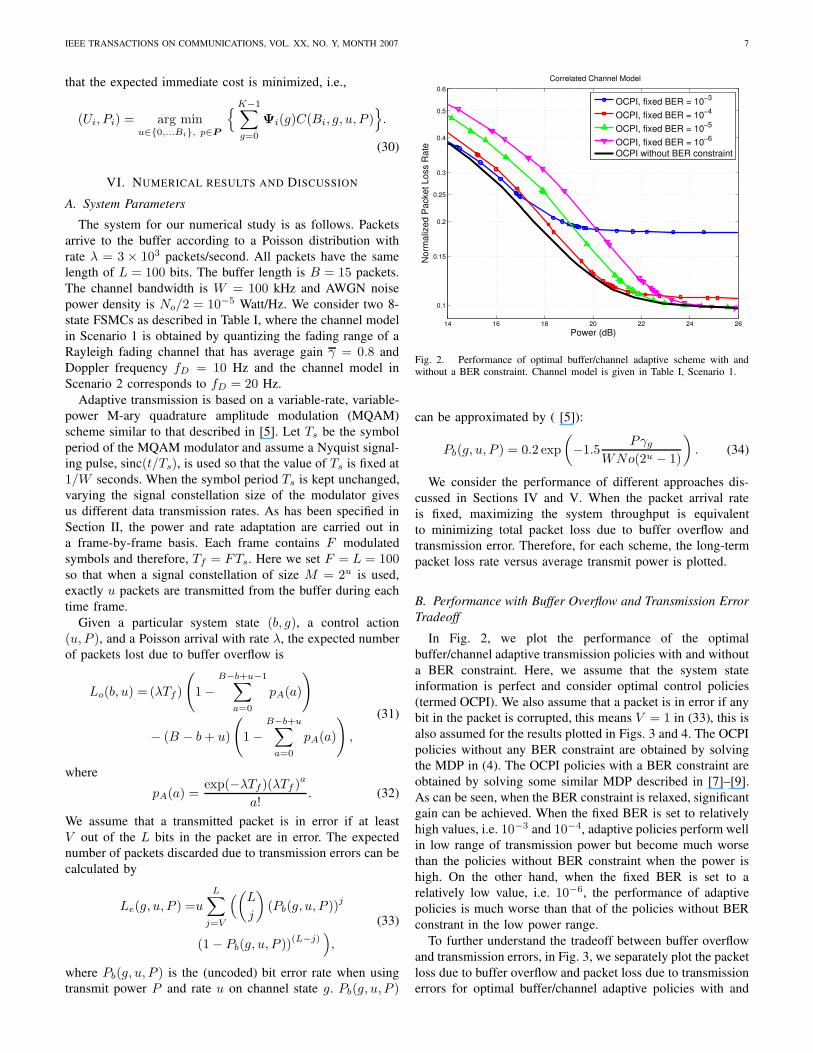
Fig. 2. Performance of optimal buffer/channel adaptive scheme with andwithout a BER constraint. Channel model is given in Table I, Scenario 1.

can be approximated by ( [5]):

Pb(g, u, P ) = 0.2 exp

(−1.5

Pγg

WNo(2u − 1)

). (34)

We consider the performance of different approaches dis-

cussed in Sections IV and V. When the packet arrival rate

is fixed, maximizing the system throughput is equivalent

to minimizing total packet loss due to buffer overflow and

transmission error. Therefore, for each scheme, the long-term

packet loss rate versus average transmit power is plotted.

B. Performance with Buffer Overflow and Transmission Error

Tradeoff

In Fig. 2, we plot the performance of the optimal

buffer/channel adaptive transmission policies with and without

a BER constraint. Here, we assume that the system state

information is perfect and consider optimal control policies

(termed OCPI). We also assume that a packet is in error if any

bit in the packet is corrupted, this means V = 1 in (33), this is

also assumed for the results plotted in Figs. 3 and 4. The OCPI

policies without any BER constraint are obtained by solving

the MDP in (4). The OCPI policies with a BER constraint are

obtained by solving some similar MDP described in [7]–[9].

As can be seen, when the BER constraint is relaxed, significant

gain can be achieved. When the fixed BER is set to relatively

high values, i.e. 10−3 and 10−4, adaptive policies perform well

in low range of transmission power but become much worse

than the policies without BER constraint when the power is

high. On the other hand, when the fixed BER is set to a

relatively low value, i.e. 10−6, the performance of adaptive

policies is much worse than that of the policies without BER

constrant in the low power range.

To further understand the tradeoff between buffer overflow

and transmission errors, in Fig. 3, we separately plot the packet

loss due to buffer overflow and packet loss due to transmission

errors for optimal buffer/channel adaptive policies with and

IEEE TRANSACTIONS ON COMMUNICATIONS, VOL. XX, NO. Y, MONTH 2007 8

TABLE I

CHANNEL STATES AND TRANSITION PROBABILITIES (AN 8-STATE FSMC OBTAINED BY QUANTIZING A RAYLEIGH FADING CHANNEL WITH AVERAGE

GAIN 0.8 AND DOPPLER FREQUENCY 10 HZ IN SCENARIO 1 AND 20 HZ IN SCENARIO 2).

Channel states k 0 1 2 3 4 5 6 7

Scenario 1 γk 0 0.1068 0.2301 0.3760 0.5545 0.7847 1.1090 1.6636Pkk 0.9359 0.8552 0.8334 0.8306 0.8420 0.8665 0.9048 0.9639

Pk,k+1 0.0641 0.0807 0.0859 0.0835 0.0745 0.0590 0.0361 0Pk,k−1 0 0.0641 0.0807 0.0859 0.0835 0.0745 0.0590 0.0361

Scenario 2 γk 0 0.1068 0.2301 0.3760 0.5545 0.7847 1.1090 1.6636Pkk 0.8718 0.7104 0.6668 0.6612 0.6841 0.7330 0.8097 0.9277

Pk,k+1 0.1282 0.1613 0.1718 0.1670 0.1489 0.1181 0.0723 0Pk,k−1 0 0.1282 0.1613 0.1718 0.1670 0.1489 0.1181 0.0723

10 12 14 16 18 20 22 24 2610

−5

10−4

10−3

10−2

10−1

100

Power (dB)

No

rma

lize

d P

acke

t L

oss R

ate

Overflow Rate (BER = 10−3

Error Rate (BER = 10−3

)

Overflow Rate (BER = 10−6

)

Error Rate (BER = 10−6

)

Overflow Rate (no BER constraint)

Error Rate (no BER constraint)

Fig. 3. Packet loss due to buffer overflow and transmission errors of optimalbuffer/channel adaptive scheme with and without a BER constraint. Channelmodel is given in Table I, Scenario 1.

without a BER constraint. It is clear that, without a BER

constraint, an optimal policy varies the transmission error

rate dynamically according to the available transmit power.

In particular, at low power, a greater number of transmission

errors can be tolerated in order to reduce buffer overflow. On

the other hand, when plenty of transmit power is available,

a good adaptive policy should transmit at a high rate and

high power to minimize both transmission errors and buffer

overflow. This argument can be further illustrated in Fig. 4,

where we plot the ratio between packet loss due to buffer

overflow and packet loss due to transmission errors.

C. Performance Under Quantized Buffer Occupancy

First, let us look at the performance of the buffer/channel

adaptive transmission approach when the buffer occupancy

is quantized. When the buffer occupancy is quantized, the

performance of policy π∗ (obtained by solving (4)) depends

on two factors, i.e., the number of quantized buffer states, and

the selected quantization thresholds. Clearly, the greater the

number of quantized states, the closer the performance to the

optimal. At the same time, given a fixed number of quantized

states, the performance depends on the set of selected thresh-

olds. An intuitive way to select good quantization thresholds

is to divide the range of buffer occupancy more finely at the

14 16 18 20 22 24 2610

0

101

102

103

104

105

Power (dB)

Ove

rflo

w_

Ra

te/E

rro

r_R

ate

Overflow/Errors (BER = 10−3

)

Overflow/Errors (BER = 10−6

)

Overflow/Errors (no BER constraint)

Fig. 4. Ratio between packet loss due to buffer overflow and packet loss dueto transmission errors of optimal adaptive scheme with and without a BERconstraint. Channel model is given in Table I, Scenario 1.

range of high probability distribution. For example, if we know

that most of the time, the buffer occupancy is low, then a

greater number of thresholds should be set at low values.

In Fig. 5, we plot the performance of π∗, in terms of total

long term packet loss rate versus average transmit power,

for different buffer quantization schemes. The number of

quantized buffer states is increased from two to four. In

particular, in the first quantization scheme, we set a single

threshold at 7. When the buffer occupancy is less than 7, it

is quantized to 0, otherwise, it is quantized to 7. Similarly,

for the case of three quantized buffer states, we set the two

thresholds at 4 and 9, and for the case of four quantized buffer

states, we set the three thresholds at 3, 6, and 10. For the

results in Fig. 5, as well as in Figs. 6-9, we assume that a

packet is in error if more than ten out of 100 bits in the

packet are corrupted, this means V = 11 in (33). As can

be seen, when only two quantized states are used, there is a

significant loss compared to the case of adapting to the exact

buffer occupancy. However, the performance loss is reduced

significantly when the number of quantized buffer states is

increased to three and four. When four quantized buffer states

are used, the performance is very near optimal. This suggests

that we can often quantize the buffer occupancy in order

to reduce the complexity of the adaptive transmission policy

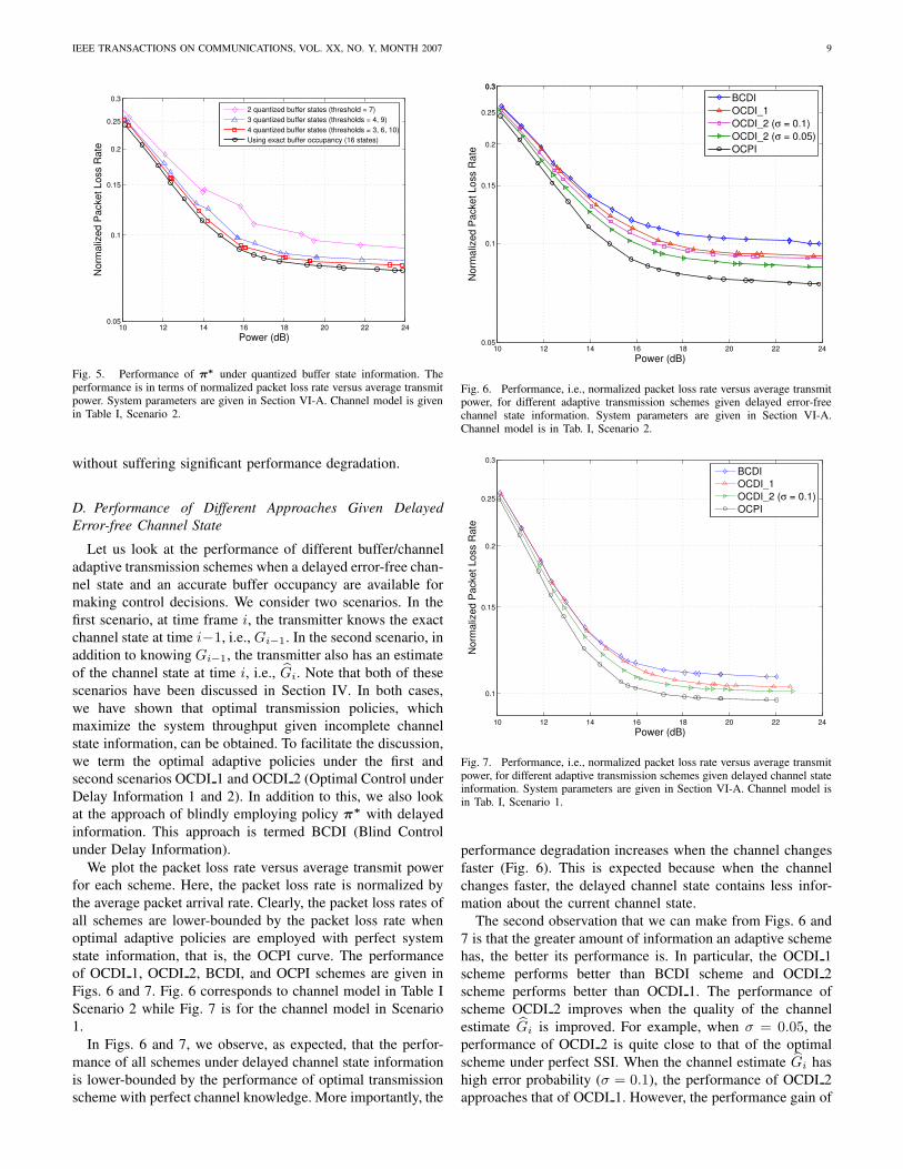
IEEE TRANSACTIONS ON COMMUNICATIONS, VOL. XX, NO. Y, MONTH 2007 9

10 12 14 16 18 20 22 240.05

0.1

0.15

0.2

0.25

0.3

Power (dB)

No

rma

lize

d P

acke

t L

oss R

ate

2 quantized buffer states (threshold = 7)

3 quantized buffer states (thresholds = 4, 9)

4 quantized buffer states (thresholds = 3, 6, 10)

Using exact buffer occupancy (16 states)

Fig. 5. Performance of π∗ under quantized buffer state information. Theperformance is in terms of normalized packet loss rate versus average transmitpower. System parameters are given in Section VI-A. Channel model is givenin Table I, Scenario 2.

without suffering significant performance degradation.

D. Performance of Different Approaches Given Delayed

Error-free Channel State

Let us look at the performance of different buffer/channel

adaptive transmission schemes when a delayed error-free chan-

nel state and an accurate buffer occupancy are available for

making control decisions. We consider two scenarios. In the

first scenario, at time frame i, the transmitter knows the exact

channel state at time i−1, i.e., Gi−1. In the second scenario, in

addition to knowing Gi−1, the transmitter also has an estimate

of the channel state at time i, i.e., Gi. Note that both of these

scenarios have been discussed in Section IV. In both cases,

we have shown that optimal transmission policies, which

maximize the system throughput given incomplete channel

state information, can be obtained. To facilitate the discussion,

we term the optimal adaptive policies under the first and

second scenarios OCDI 1 and OCDI 2 (Optimal Control under

Delay Information 1 and 2). In addition to this, we also look

at the approach of blindly employing policy π∗ with delayed

information. This approach is termed BCDI (Blind Control

under Delay Information).

We plot the packet loss rate versus average transmit power

for each scheme. Here, the packet loss rate is normalized by

the average packet arrival rate. Clearly, the packet loss rates of

all schemes are lower-bounded by the packet loss rate when

optimal adaptive policies are employed with perfect system

state information, that is, the OCPI curve. The performance

of OCDI 1, OCDI 2, BCDI, and OCPI schemes are given in

Figs. 6 and 7. Fig. 6 corresponds to channel model in Table I

Scenario 2 while Fig. 7 is for the channel model in Scenario

1.

In Figs. 6 and 7, we observe, as expected, that the perfor-

mance of all schemes under delayed channel state information

is lower-bounded by the performance of optimal transmission

scheme with perfect channel knowledge. More importantly, the

10 12 14 16 18 20 22 240.05

0.1

0.15

0.2

0.25

0.30.3

Power (dB)

Norm

aliz

ed P

acket Loss R

ate

BCDI

OCDI_1

OCDI_2 (σ = 0.1)

OCDI_2 (σ = 0.05)

OCPI

Fig. 6. Performance, i.e., normalized packet loss rate versus average transmitpower, for different adaptive transmission schemes given delayed error-freechannel state information. System parameters are given in Section VI-A.Channel model is in Tab. I, Scenario 2.

10 12 14 16 18 20 22 24

0.1

0.15

0.2

0.25

0.3

Power (dB)

Norm

aliz

ed P

acket Loss R

ate

BCDI

OCDI_1

OCDI_2 (σ = 0.1)

OCPI

Fig. 7. Performance, i.e., normalized packet loss rate versus average transmitpower, for different adaptive transmission schemes given delayed channel stateinformation. System parameters are given in Section VI-A. Channel model isin Tab. I, Scenario 1.

performance degradation increases when the channel changes

faster (Fig. 6). This is expected because when the channel

changes faster, the delayed channel state contains less infor-

mation about the current channel state.

The second observation that we can make from Figs. 6 and

7 is that the greater amount of information an adaptive scheme

has, the better its performance is. In particular, the OCDI 1

scheme performs better than BCDI scheme and OCDI 2

scheme performs better than OCDI 1. The performance of

scheme OCDI 2 improves when the quality of the channel

estimate Gi is improved. For example, when σ = 0.05, the

performance of OCDI 2 is quite close to that of the optimal

scheme under perfect SSI. When the channel estimate Gi has

high error probability (σ = 0.1), the performance of OCDI 2

approaches that of OCDI 1. However, the performance gain of

IEEE TRANSACTIONS ON COMMUNICATIONS, VOL. XX, NO. Y, MONTH 2007 10

10 12 14 16 18 20 220.05

0.1

0.15

0.2

0.25

0.30.3

Power (dB)

Norm

aliz

ed P

acket Loss R

ate

MIC

BCEI

MLS

QMDP

OCPI

Fig. 8. Performance, i.e., normalized packet loss rate versus average transmitpower, for different adaptive transmission schemes given imperfect channelestimate. System parameters are given in Section VI-A. Channel model isin Tab. I, Scenario 2. The standard deviation of channel estimating noise isσ = 0.05.

OCDI 2 comes at a cost of higher complexity. In particular,

the number of internal channel states for OCDI 2 is K2 while

it is K for OCDI 1.

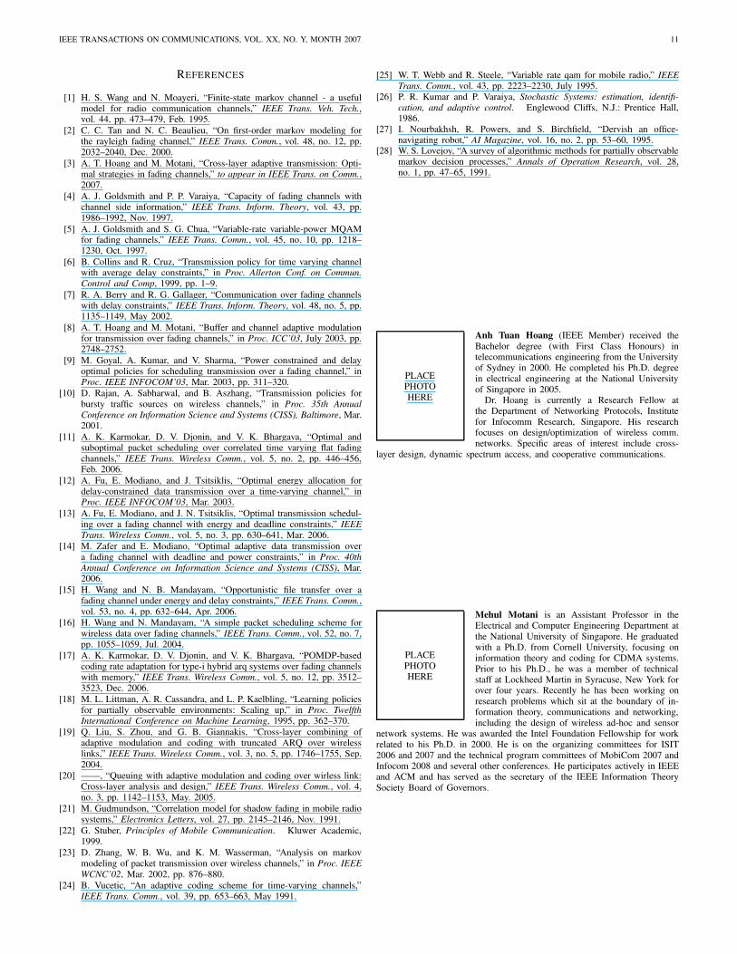
E. Performance of Different Approaches Given Imperfect

Channel Estimates

Now let us look at the performance of different buffer

and channel adaptive transmission schemes when no error-

free channel state information is available at the transmitter.

In particular, during time slot i, the transmitter only has an

estimate of the channel state, i.e., Gi. For this numerical study,

we assume that the estimation error for the channel gain has

a Gaussian distribution with zero mean and variation of σ2.

The estimation statistics can be computed using equation (11)

- (13).

As has been discussed in Section V-B, for the general

case of correlated channel model, when no perfect channel

estimate is available at the transmitter, it is not practical to

look for optimal adaptive transmission policies. Instead, there

are various approaches that can approximate optimal control

policies at lower complexity. These approaches are: BCEI,

MLS, QMDP and they have been discussed in Section V-B.

Note that BCEI is the approach that blindly employs policy

π∗ with erroneous channel state information. Again, we plot

the performance of different adaptive schemes in terms of

normalized packet loss rate versus average transmit power. The

performance of all schemes are compared to the case when an

optimal scheme is employed under perfect SSI, that is, the

OCPI curve. The performance of different classes of adaptive

policies is given in Figs. 8 and 9. Fig. 8 is obtained for the

case when σ = 0.05 and Fig. 9 is for the case when σ = 0.1.

In both Figs. 8 and 9, the channel model in Table I, Scenario

2, is used.

As can be seen, the MIC approach, which only tries to

minimize the immediate cost during each time frame and does

10 12 14 16 18 20 220.05

0.1

0.15

0.2

0.25

0.3

0.35

0.40.4

Power (dB)

Norm

aliz

ed P

acket Loss R

ate

MIC

BCEI

MLS

QMDP

OCPI

Fig. 9. Performance, i.e., normalized packet loss rate versus average transmitpower, for different adaptive transmission schemes given imperfect channelestimate. System parameters are given in Section VI-A. Channel model isin Tab. I, Scenario 2. The standard deviation of channel estimating noise isσ = 0.1.

not take the dynamics of the system into account has the worst

performance. Significant performance gain can be achieved by

using BCEI, MLS, and QMDP approaches. This shows the

important of structuring the problem as a partially observable

Markov decision process.

Among the three approaches BCEI, MLS, and QMDP, it

seems that QMDP performs best. We note that there is no

significant extra complexity when using QMDP instead of

BCEI or MLS, therefore, QMDP is a good choice to cope with

imperfect estimated channel state information. Between BCEI

and MLS, MLS tends to perform better at low power range,

while at higher power range, BCEI achieves better results.

However, we note that the difference in the performance

of BCEI and MLS is not significant, therefore, the simpler

approach, i.e., BCEI, is preferable.

VII. CONCLUSION

In this paper, we consider the problem of buffer and channel

adaptive transmission for maximizing the throughput of a

transmission over a wireless fading channel, subject to an

average transmit power constraint. We consider scenarios in

which the system state information for making control deci-

sions is incomplete. This includes delayed and/or imperfectly

estimated channel state and quantized buffer occupancy. We

also allow for a tradeoff due to the loss from both transmission

errors and buffer overflow and obtain significant throughput

improvement.

This paper shows the importance of cross-layer design in

achieving good performance for wireless data communication

system. This paper also demonstrates that, even when the sys-

tem state is not fully observable, buffer and channel adaptive

transmission can still be implemented in an effective manner.

IEEE TRANSACTIONS ON COMMUNICATIONS, VOL. XX, NO. Y, MONTH 2007 11

REFERENCES

[1] H. S. Wang and N. Moayeri, “Finite-state markov channel - a usefulmodel for radio communication channels,” IEEE Trans. Veh. Tech.,vol. 44, pp. 473–479, Feb. 1995.

[2] C. C. Tan and N. C. Beaulieu, “On first-order markov modeling forthe rayleigh fading channel,” IEEE Trans. Comm., vol. 48, no. 12, pp.2032–2040, Dec. 2000.

[3] A. T. Hoang and M. Motani, “Cross-layer adaptive transmission: Opti-mal strategies in fading channels,” to appear in IEEE Trans. on Comm.,2007.

[4] A. J. Goldsmith and P. P. Varaiya, “Capacity of fading channels withchannel side information,” IEEE Trans. Inform. Theory, vol. 43, pp.1986–1992, Nov. 1997.

[5] A. J. Goldsmith and S. G. Chua, “Variable-rate variable-power MQAMfor fading channels,” IEEE Trans. Comm., vol. 45, no. 10, pp. 1218–1230, Oct. 1997.

[6] B. Collins and R. Cruz, “Transmission policy for time varying channelwith average delay constraints,” in Proc. Allerton Conf. on Commun.

Control and Comp, 1999, pp. 1–9.

[7] R. A. Berry and R. G. Gallager, “Communication over fading channelswith delay constraints,” IEEE Trans. Inform. Theory, vol. 48, no. 5, pp.1135–1149, May 2002.

[8] A. T. Hoang and M. Motani, “Buffer and channel adaptive modulationfor transmission over fading channels,” in Proc. ICC’03, July 2003, pp.2748–2752.

[9] M. Goyal, A. Kumar, and V. Sharma, “Power constrained and delayoptimal policies for scheduling transmission over a fading channel,” inProc. IEEE INFOCOM’03, Mar. 2003, pp. 311–320.

[10] D. Rajan, A. Sabharwal, and B. Aszhang, “Transmission policies forbursty traffic sources on wireless channels,” in Proc. 35th Annual

Conference on Information Science and Systems (CISS), Baltimore, Mar.2001.

[11] A. K. Karmokar, D. V. Djonin, and V. K. Bhargava, “Optimal andsuboptimal packet scheduling over correlated time varying flat fadingchannels,” IEEE Trans. Wireless Comm., vol. 5, no. 2, pp. 446–456,Feb. 2006.

[12] A. Fu, E. Modiano, and J. Tsitsiklis, “Optimal energy allocation fordelay-constrained data transmission over a time-varying channel,” inProc. IEEE INFOCOM’03, Mar. 2003.

[13] A. Fu, E. Modiano, and J. N. Tsitsiklis, “Optimal transmission schedul-ing over a fading channel with energy and deadline constraints,” IEEE

Trans. Wireless Comm., vol. 5, no. 3, pp. 630–641, Mar. 2006.

[14] M. Zafer and E. Modiano, “Optimal adaptive data transmission overa fading channel with deadline and power constraints,” in Proc. 40th

Annual Conference on Information Science and Systems (CISS), Mar.2006.

[15] H. Wang and N. B. Mandayam, “Opportunistic file transfer over afading channel under energy and delay constraints,” IEEE Trans. Comm.,vol. 53, no. 4, pp. 632–644, Apr. 2006.

[16] H. Wang and N. Mandayam, “A simple packet scheduling scheme forwireless data over fading channels,” IEEE Trans. Comm., vol. 52, no. 7,pp. 1055–1059, Jul. 2004.

[17] A. K. Karmokar, D. V. Djonin, and V. K. Bhargava, “POMDP-basedcoding rate adaptation for type-i hybrid arq systems over fading channelswith memory,” IEEE Trans. Wireless Comm., vol. 5, no. 12, pp. 3512–3523, Dec. 2006.

[18] M. L. Littman, A. R. Cassandra, and L. P. Kaelbling, “Learning policiesfor partially observable environments: Scaling up,” in Proc. Twelfth

International Conference on Machine Learning, 1995, pp. 362–370.

[19] Q. Liu, S. Zhou, and G. B. Giannakis, “Cross-layer combining ofadaptive modulation and coding with truncated ARQ over wirelesslinks,” IEEE Trans. Wireless Comm., vol. 3, no. 5, pp. 1746–1755, Sep.2004.

[20] ——, “Queuing with adaptive modulation and coding over wirless link:Cross-layer analysis and design,” IEEE Trans. Wireless Comm., vol. 4,no. 3, pp. 1142–1153, May. 2005.

[21] M. Gudmundson, “Correlation model for shadow fading in mobile radiosystems,” Electronics Letters, vol. 27, pp. 2145–2146, Nov. 1991.

[22] G. Stuber, Principles of Mobile Communication. Kluwer Academic,1999.

[23] D. Zhang, W. B. Wu, and K. M. Wasserman, “Analysis on markovmodeling of packet transmission over wireless channels,” in Proc. IEEE

WCNC’02, Mar. 2002, pp. 876–880.

[24] B. Vucetic, “An adaptive coding scheme for time-varying channels,”IEEE Trans. Comm., vol. 39, pp. 653–663, May 1991.

[25] W. T. Webb and R. Steele, “Variable rate qam for mobile radio,” IEEE

Trans. Comm., vol. 43, pp. 2223–2230, July 1995.[26] P. R. Kumar and P. Varaiya, Stochastic Systems: estimation, identifi-

cation, and adaptive control. Englewood Cliffs, N.J.: Prentice Hall,1986.

[27] I. Nourbakhsh, R. Powers, and S. Birchfield, “Dervish an office-navigating robot,” AI Magazine, vol. 16, no. 2, pp. 53–60, 1995.

[28] W. S. Lovejoy, “A survey of algorithmic methods for partially observablemarkov decision processes,” Annals of Operation Research, vol. 28,no. 1, pp. 47–65, 1991.

PLACEPHOTOHERE

Anh Tuan Hoang (IEEE Member) received theBachelor degree (with First Class Honours) intelecommunications engineering from the Universityof Sydney in 2000. He completed his Ph.D. degreein electrical engineering at the National Universityof Singapore in 2005.

Dr. Hoang is currently a Research Fellow atthe Department of Networking Protocols, Institutefor Infocomm Research, Singapore. His researchfocuses on design/optimization of wireless comm.networks. Specific areas of interest include cross-

layer design, dynamic spectrum access, and cooperative communications.

PLACEPHOTOHERE

Mehul Motani is an Assistant Professor in theElectrical and Computer Engineering Department atthe National University of Singapore. He graduatedwith a Ph.D. from Cornell University, focusing oninformation theory and coding for CDMA systems.Prior to his Ph.D., he was a member of technicalstaff at Lockheed Martin in Syracuse, New York forover four years. Recently he has been working onresearch problems which sit at the boundary of in-formation theory, communications and networking,including the design of wireless ad-hoc and sensor

network systems. He was awarded the Intel Foundation Fellowship for workrelated to his Ph.D. in 2000. He is on the organizing committees for ISIT2006 and 2007 and the technical program committees of MobiCom 2007 andInfocom 2008 and several other conferences. He participates actively in IEEEand ACM and has served as the secretary of the IEEE Information TheorySociety Board of Governors.