An Efficient Fuzzy Clustering-Based Approach

for Intrusion Detection

Huu Hoa Nguyen, Nouria Harbi and Jérôme Darmont

Université de Lyon (ERIC Lyon 2) - France

nhhoa@eric.univ-lyon2.fr, {nouria.harbi, jerome.darmont}@univ-lyon2.fr

Abstract. The need to increase accuracy in detecting sophisticated cyber

attacks poses a great challenge not only to the research community but also to

corporations. So far, many approaches have been proposed to cope with this

threat. Among them, data mining has brought on remarkable contributions to

the intrusion detection problem. However, the generalization ability of data

mining-based methods remains limited, and hence detecting sophisticated

attacks remains a tough task. In this thread, we present a novel method based on

both clustering and classification for developing an efficient intrusion detection

system (IDS). The key idea is to take useful information exploited from fuzzy

clustering into account for the process of building an IDS. To this aim, we first

present cornerstones to construct additional cluster features for a training set.

Then, we come up with an algorithm to generate an IDS based on such cluster

features and the original input features. Finally, we experimentally prove that

our method outperforms several well-known methods.

Keywords: classification, fuzzy clustering, intrusion detection, cyber attack.

1 Introduction

In recent years, with the dramatically increasing use of network-based services and

the vast spectrum of information technology security breaches, more and more

organizational information systems are subject to attack by intruders. Among many

approaches proposed in the literature to deal with this threat, data mining brings on a

noticeable success to the development of high performance intrusion detection

systems (IDSs). The preeminence of such an approach lies in its good generalization

abilities to correctly classify (or detect) both known and unknown attacks. However,

as an inherent essence, the effectiveness of data mining-based IDSs depends heavily

upon the quality of IDS datasets. In practice, IDS datasets are often extracted from

raw traces in a chaotic system environment, and hence could hold implicit

deficiencies, e.g., the existence of noise in class labels due to mistakes in

measurement, and the lack of base features. Moreover, due to the sophisticated

characteristics of attacks and the diversification of normal events, different data

regions could behave differently, i.e., true class labels could seriously be interlaced.

Such factors pose a great difficulty for inducers to identify appropriate decision

boundaries from the input space of IDS datasets. In other words, when the input space

is not robust enough to discriminate class labels, making further treatments from

alternative knowledge sources as new supplemental features is highly desirable. To

this aim, one common approach is to transform the input space into a higher

dimensional space from which data are more separable. New additional features can

be found by either manual ways based on prior knowledge or automatic analysis

methods (e.g., principle component analysis). However, in a high dimensional input

space, finding new relevant features is a tough task that often requires human

analyses, but derived features are sometimes not as good as expected. As a result, in

practice, one often applies standard dimensional-transformation methods (e.g.,

polynomial, radial basic function) to application domains where class discrimination

is ambiguous and additional features are hard to be identified. Yet, such methods are

greatly affected by input parameters and data distribution, thus not always outputting

a high performance classifier. In this vision, it is desirable to find additional features

in a less complex way so that general-purpose algorithms such as Decision Trees

(DT) or Support Vector Machines (SVM) can learn the data more efficiently.

Such a context motivates us to propose a novel approach that treats fuzzy cluster

information as additional features. These features are selectively incorporated into the

input space for building an efficient IDS. we experimentally show that our solution

approach is considerably superior to several well-known methods.

The remainder of this paper is organized as follows. Section 2 presents the

problem formulation of our approach, whereas section 3 describes our solution for

generating an IDS. Section 4 shows the experimental results we achieved. Section 5

finally gives a conclusion of the method we propose.

2 Problem formulation

Clustering aims to organize data into groups (clusters) according to their similarities

measured by some concepts. Unlike crisp clustering that crisply assigns each data

point to a separate cluster, fuzzy clustering allows each data point to belong to various

clusters with different membership degrees (or weights). Fuzzy clusters are expressed

by their centers (or centroids) that are simultaneously found in the partitioning

process of a fuzzy clustering algorithm. The number of clusters (k) is often inputted as

a parameter to a fuzzy clustering algorithm. The nk membership matrix W={wij

[0,1]} of n data points is found in the fuzzy clustering process. For example, Figure 1

describes the instance space of a training set partitioned into four fuzzy clusters,

where membership weights that data point x1 belongs to clusters '1', '2', '3', and '4' are

0.3, 0.14, 0.16, and 0.4, respectively.

Let us first denote S={X,Y} the original training set of n data points X={x1,…,xn},

where each point xi is an m-dimensional vector (xi1,…,xim) and assigned to a label

yiY belonging one of the c classes ={1, …,c}. Let B={bi| bi=max(wij), j=1…k}

hold the maximum membership weight of each point xi, and Z={zi| zi=argmaxj(wij),

j=1…k } contains the cluster (symbolic) number assigned to each point xi.

For conciseness in describing the approach, we term two column matrices Z and B

as two “basic cluster features”. In addition, we name the jth

column of the membership

matrix (W) as Pj, and term the columns P1, ..., Pk as “extended cluster features”. We

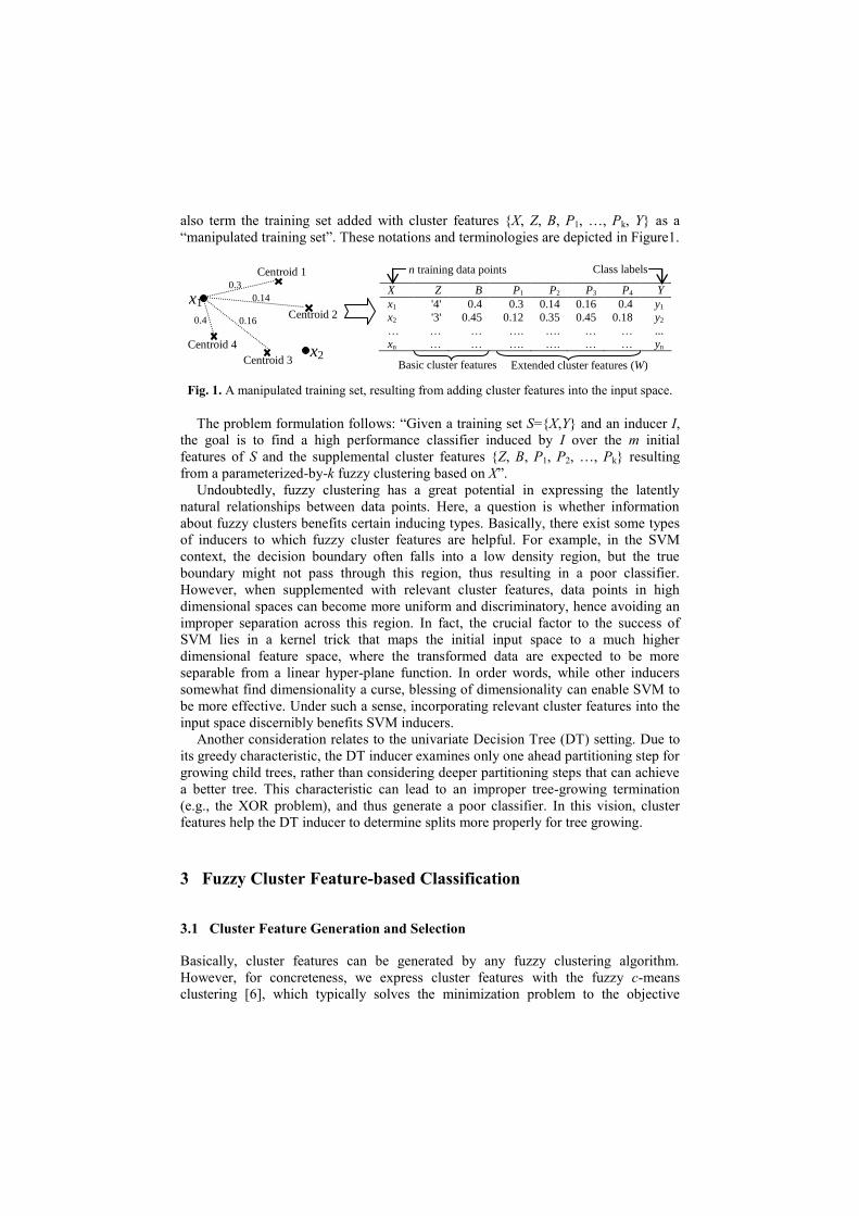
also term the training set added with cluster features {X, Z, B, P1, …, Pk, Y} as a

“manipulated training set”. These notations and terminologies are depicted in Figure1.

X Z B P1 P2 P3 P4 Y

x1 '4' 0.4 0.3 0.14 0.16 0.4 y1

x2 '3' 0.45 0.12 0.35 0.45 0.18 y2

… … … …. …. … … ...

xn … … …. …. … … yn

Basic cluster features Extended cluster features (W)

Class labels n training data points Centroid 1

Centroid 2

Centroid 3

Centroid 4

x1

x2

0.3

0.14

0.16 0.4

Fig. 1. A manipulated training set, resulting from adding cluster features into the input space.

The problem formulation follows: “Given a training set S={X,Y} and an inducer I,

the goal is to find a high performance classifier induced by I over the m initial

features of S and the supplemental cluster features {Z, B, P1, P2, …, Pk} resulting

from a parameterized-by-k fuzzy clustering based on X”.

Undoubtedly, fuzzy clustering has a great potential in expressing the latently

natural relationships between data points. Here, a question is whether information

about fuzzy clusters benefits certain inducing types. Basically, there exist some types

of inducers to which fuzzy cluster features are helpful. For example, in the SVM

context, the decision boundary often falls into a low density region, but the true

boundary might not pass through this region, thus resulting in a poor classifier.

However, when supplemented with relevant cluster features, data points in high

dimensional spaces can become more uniform and discriminatory, hence avoiding an

improper separation across this region. In fact, the crucial factor to the success of

SVM lies in a kernel trick that maps the initial input space to a much higher

dimensional feature space, where the transformed data are expected to be more

separable from a linear hyper-plane function. In order words, while other inducers

somewhat find dimensionality a curse, blessing of dimensionality can enable SVM to

be more effective. Under such a sense, incorporating relevant cluster features into the

input space discernibly benefits SVM inducers.

Another consideration relates to the univariate Decision Tree (DT) setting. Due to

its greedy characteristic, the DT inducer examines only one ahead partitioning step for

growing child trees, rather than considering deeper partitioning steps that can achieve

a better tree. This characteristic can lead to an improper tree-growing termination

(e.g., the XOR problem), and thus generate a poor classifier. In this vision, cluster

features help the DT inducer to determine splits more properly for tree growing.

3 Fuzzy Cluster Feature-based Classification

3.1 Cluster Feature Generation and Selection

Basically, cluster features can be generated by any fuzzy clustering algorithm.

However, for concreteness, we express cluster features with the fuzzy c-means

clustering [6], which typically solves the minimization problem to the objective

function of Formula 1. In a common form, the objective function (Formula 1) reaches

to a minimum over W (membership matrix) and V (centroids), by Formulas 2 and 3.

2

1 1

( , , ) ( , )

k n

obj ij i j

j i

f X W V w d x v

, subject to the constrain 1

1

k

ij

j

w

(1)

1 1

( ) ( )

n n

j ij i ij

i i

v w x w

(2)

1 1

1 1

2 2

1

1 1

( , ) ( , )

k

ij

qi j i q

wd x v d x v

(3)

where is a fuzzy constant and d(xi,vj) is the distance from xi (X ) to vj (V)

Fuzzy c-means clustering tries to find the best fit for a fixed value of k, the number

of clusters. However, as an essential problem of clustering, determining an

appropriate parameter k is a tough task. The most common way to find the reasonable

number of clusters is to run the clustering with various values of k {2,…, kmax} and

then use a validity measure (e.g., partition coefficient ) to evaluate cluster fitness.

In our approach, however, we need data to be grouped in a way that reveals helpful

information for inducers, not for clustering itself, even though the number of clusters

might be wrong. In other words, using validity measures to determine the best number

of clusters is not reliable enough to derive good cluster features for classifiers. In such

a vision, instead of endeavoring to find the best k with validity measures, we use the

over-production method to generate several candidate classifiers for different values

of k and then evaluate their performance to determine the best one. Evaluating the

performance of candidate classifiers can be based either on a validation set or Cross

Validation (CV) method [9]. Thus, a proper value of k is simultaneously found in the

process of finding a maximum performance classifier from candidate classifiers.

In addition, the use of cluster features should be examined individually for a

concrete inducing type. Intuitively, two basic cluster features (Z, B) are benefic

enough for DT inducer, instead of including k extended cluster features (P1,…,Pk). By

contrast, in the SVM context, it is applicable to employ either only the basic cluster

features (Z, B) or all the cluster features (Z, B, P1,…,Pk) for building a classifier.

Another solution that can be applied for any inducing type is to employ feature

selection techniques (e.g., filter, wrapper) to pick out high merit features from both m

initial input features and all (k+2) cluster features. The objective is to apply feature

selection techniques on (m+k+2) features to bring about a smaller but more qualitative

feature subset than those only on m initial features. Here, note is that feature selection

is simultaneously carried out in the process of building candidate classifiers. In a

nutshell, formally, there are three possibilities to incorporate cluster features into the

initial features (A1, …, Am), i.e., (A1, …, Am, Z, B), (A1, …, Am, Z, B, P1, …, Pk), or

Feature Selection(A1, …, Am, Z, B, P1, …, Pk).

3.2 Algorithm for generating a fuzzy cluster feature-based classifier

Our algorithm for generating a classifier from both initial and cluster features, called

CFC, is depicted from Figure 2. Related notations are indicated in Table 1.

Table 1. Notations used in Figure 2.

Notation Description

Ck A candidate classifier resulting from a clustering with k fuzzy clusters.

Ck* The best classifier among |K| candidate classifiers.

Vk A k m matrix of k centroids obtained from clustering X into k clusters.

Vk* A k* m matrix of k* centroids, corresponding to Ck*.

Wk An n k membership matrix of n data points xi X, corresponding to Vk.

kB A column matrix containing the maximum membership weight of each xi X.

kZ A column matrix representing the cluster (symbolic) number of each xi X.

A horizontal concatenation operator between two matrices.

Training phase

Input: S={X, Y}: The original training set

I: a base inducer

K: a predefined integer set representing possible number of clusters

: a feature selection technique that returns a specific feature subset

T: a type to employ features for building classifiers

Output: *k

C , *kV

1: Normalize( )X X //Normalize continuous features

2: For each k K do

3: { , } FuzzyC lustering ( , )k k

W V X k

4: { | m ax( ), 1 ... , 1 ... }k

i i ijB b b w i n j k

5: { | arg m ax ( ), 1 ... , 1 ... }k

i i j ijZ z z w i n j k

6: Case //D is a manipulated training set

7: T = 1: ( )k k

D X Z B //Initial features & basic cluster features

8: T = 2: ( )k k k

D X Z B W //Initial features & all cluster features

9: T = 3:

( , )k k k

F X Z B W Y //Apply a feature selection

( )k k k

D X Z B W [F] //Project data by the derived subset

10: End Case

11: ( , )k

C I D Y //Build a classifier, using the manipulated training set D & inducer I

12: Performance( )k

C {Average performance of q-fold CV based on (D,Y) and I }

13: End For

14:*

arg m ax Perform ance( ),kk C k

C C k K //Determine one best classifier

15: Return *

*,

k

kC V

Operation phase

16: For an unlabeled testing instance x:

17: Normalize( )x x //Normalize continuous features

18: Compute membership weights ( | 1... *)jw j k that x belongs to *k

jv V (Formula 3)

19: max( | 1... *)jb w j k

20: arg max ( | 1... *)j jz w j k

21: Label x, by taking cluster features { , , }jz b w into account, using *k

C

Fig. 2. Algorithm CFC.

The key idea is that, for each clustering with different number of clusters (kK),

the algorithm builds and valuates a candidate classifier from the training set

manipulated with a given feature selection type, by q-Fold Cross Validation [9]. The

resulting classifier is the one exhibiting maximum performance.

In the training phase, the algorithm first normalizes continuous features (e.g., by a

variance-based spread measure) to avoid the dispersion in different ranges (Line 1).

Here, it is noticed that the normalized data (X) is merely for clustering purpose,

whereas classifiers are built by using the original data (X). In addition, instead of

executing clustering with parameter k ranging from 2 to a given kmax value, the

algorithm uses a predefined set K={k} to mainly focus on important values of k,

which can be recognized by experiment or prior knowledge (Line 2). As mentioned in

Section 3.1, there are three cases to incorporate cluster features into the initial

features. Hence, for general purpose, the algorithm introduces an input parameter T

for specifying the way to employ features for building classifiers (Lines 6-10).

Subsequently, the algorithm builds and evaluates one candidate classifier for each

clustering (Lines 11, 12). Here, note is that evaluating candidate classifiers is based

on the averaged performance of q-fold stratified cross validation from the

manipulated training set. Finally, the algorithm determines one best classifier from |K|

candidate classifiers, together with a corresponding centroid set (Lines 14, 15).

In the operation phase, for an unlabeled testing instance x, the algorithm first

normalizes x in the same way as those applied to the training set. Then, cluster

features of x are calculated based on the centroid set *kV (Lines 18-20). Finally, the

corresponding features are input to classifier *k

C for final prediction (Line 21).

4 Experiments

4.1 Dataset

Our experiments are conducted on the intrusion detection dataset KDD99 [3]. This

dataset was derived from the DARPA dataset, a format of TCPdump files captured

from the simulation of normal and attack activities in the network environment of an

air-force base, created by MIT’s Lincoln Laboratory. The KDD99 dataset comprises

494,021 training instances and 311,029 testing instances. Due to data volume, the

research community mostly uses small subsets of the dataset for evaluating IDS

methods. Each instance in the dataset represents a network connection, i.e., a

sequence of network packets starting and ending at some well defined times, between

which data flows to and from a source IP address to a target IP address under some

well defined protocol. Such a connection instance is described by a 41-dimensional

feature vector and labeled with respect to five classes: Normal, Probe, DoS (denial of

service), R2L (remote to local), and U2R (user to root).

To facilitate experiments without losing generality, we only use a smaller set of the

KDD99 dataset for the purpose of evaluating and comparing our method to others. In

particular, the training and testing sets used in our experiments are made up of 33,016

instances and 169,687 instances that are selectively extracted from the KDD99

training and testing sets, respectively. The principle for forming such reduced sets is

to get all instances in each small group (attack type), but only a limited amount of

instances in each large group, from both the KDD99 training and testing sets. More

explicitly, for forming the reduced training, we randomly select five percent of each

large group Neptune, smurf, and normal, while gathering all instances in the

remaining groups from the KDD99 training set. For sampling the reduced testing set,

we randomly select 50 percent of each large group Neptune, smurf, and normal,

whereas collecting all instances in the remaining groups from the KDD99 testing set.

Class distribution of these two reduced sets is shown in Table 2.

Table 2. Class distribution of the reduced training and testing sets used in experiments.

Class Training set Testing set Class Training set Testing set

DoS 22,867 118,807 U2R 52 70

Probe 4,107 4,166 Normal 4,864 30,297

R2L 1,126 16,347 Total 33,016 169,687

4.2 Experiment Setup

In our experiments, the predefined set K is set to {2, 3, …, 50}. The convergence

criterion (termination tolerance) of fuzzy c-means clustering is set to 10-6

, whereas the

fuzzy degree (exponent in Formulas 1-3) is set to 3. On the other hand, continuous

futures are normalized by max_min value ranges [6]. To handle different feature types

as well as express different merit contributions of features in the Euclidian space, we

calculate distances between data points by the metric proposed in Formula 4.

2 2

( , ) ( , )

m

i j q q iq jq

q

d x v G d x v (4)

where Gq is information gain of feature q [5], and

1, , {sym bolic} ( ) , {unknow n}

| |, , {continuous}

( , )| |

, , {ordinals}; {ordinals}1

0, otherw ise,

iq jq iq jq iq jq

iq jq iq jq

q iq jqiq jq

iq jq

if x v x v or x v

x v if x v

d x v x vif x v t

t

The base inducers (I) tested in our method are the C4.5 decision tree [5] and the

SVM [2] with polynomial and radial basic function kernels. The feature selection

technique () used in this experiment is Correlation-based Feature Subset Evaluation

(CfsSubsetEval) with genetic search [7]. CfsSubsetEval evaluates the merit of a

feature subset by considering the individual predictive ability of each feature along

with the degree of redundancy between them. Those subsets that are highly correlated

with the class while having low intercorrelation are preferred.

Candidate classifiers are evaluated by an attack type-based stratified cross

validation (q=10 folds). The maximum performance classifier is determined based on

overall accuracy (i.e., the ratio of the number of correctly classified instances to the

total number of instances in the training set).

4.3 Experiment Results

The experimental comparison of our method to other well-known methods is featured

in Table 3. All the compared classifiers are built from the same training set and tested

on the same testing set as described in Section 4.1. Moreover, Figure 4 depicts True

Positive Rates (TPRs) and False Positive Rates (FPRs) of classifiers with respect to

each class label, whereas Figure 3 portrays average TPRs and FPRs of classifiers.

TPR of a class c is the ratio of “the number of correctly classified instances in the

class c” to “the total number of instances in the class c”. FPR of a class c is the

ratio of “the number of instances that do not belong to the class c but are classified

as c” to “the total number of instances that do not belong to the class c”.

To have a wider comparative view, we run our algorithm (CFC) with different

settings of two parameters (i.e., I: base inducer; T: the way to employ cluster features

for building classifiers). The results of such runs are listed in Rows 10-18 of Table 3.

As shown in Figures 3 and 4, our method, in general, considerably outperforms the

others with respect to TPRs in all five classes and on average. Particularly, CFC

classifiers are significantly better than all the others in detecting hard classes (i.e.,

R2L and U2R). On the other hand, FPRs of CFC classifiers are generally lower than

those of the others. Our method also considerably improves the classification ability

of base inducers (SVM and DT) in both viewpoints, i.e., applying or not applying

feature selection. More concretely, by using the same feature selection technique, the

SVM classifier built from the manipulated training set (i.e., CFC(I=SVM,T=3)) is

considerably superior to the SVM classifier built from the original training set (i.e.,

SVM_FS). Similarly, the performance of CFC(I=DT,T=3) is considerably better than

that DT_FS. This tells that applying a feature selection technique on the manipulated

training set produces a higher qualitative feature subset (including base features and

cluster features) than that on the original training set.

Regarding the SVM context, although we further test PSVM (Polynomial SVM)

with exponent degrees ranging from 2 to 6, its performance remains worse than

CFC(PSVM(degree=2),T={1,2,3}). On average, CFC(PSVM (degree=2),T={1,2,3})

gives a 91.96% TPR (with a 2.2% FPR), whereas PSVM(degree={2,…,6}) produces

an 86.84% TPR (with a 3.44% FPR). We also test RSVM (Radial Basic Function

SVM) with widths Gamma ranging from 0.1 to 1.0, but its performance still

underperforms CFC(RSVM(Gamma=0.1),T={1,2,3}). More precisely, on average,

RSVM(Gamma={0.1,0.2,...,1}) produces an 86.72% TPR (with a 3.62% FPR),

whereas CFC(RSVM(Gamma=0.1),T={1,2,3}) gives a 91.15% TPR (with a 2.3%

FPR). This tells that cluster features benefit SVM in high dimensionality.

87.05 86.27 86.69 86.18 86.49 87.03 86.94 87.02 87.09 90.89 90.18 91.49 91.70 91.24 92.92 90.37 90.96 92.12

3.00 5.82 3.20 4.68 3.25 3.27 5.03 3.32 4.61 2.35 2.90 2.16 2.18 2.35 2.08 2.45 2.38 2.070102030405060708090

100

TPR

FPR

Fig. 3. Average True Positive and False Positive Rates (%) of classifiers

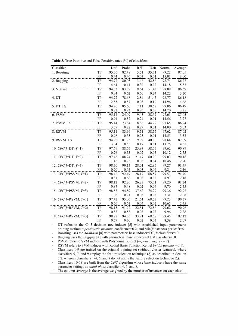
Table 3. True Possitive and False Possitive rates (%) of classifiers.

Classifier DoS Probe R2L U2R Normal Average

1. Boosting TP 95.36 82.48 5.51 35.71 99.22 87.05

FP 0.44 0.46 0.03 0.01 15.01 3.00

2. Bagging TP 94.72 80.03 3.46 42.86 98.74 86.27

FP 4.64 0.41 0.30 0.02 14.18 5.82

3. NBTree TP 94.53 83.32 9.54 51.43 98.08 86.69

FP 0.84 0.62 0.60 0.24 14.22 3.20

4. DT TP 94.72 78.68 2.84 51.43 98.77 86.18

FP 2.85 0.57 0.03 0.10 14.96 4.68

5. DT_FS TP 94.26 85.60 7.11 38.57 99.06 86.49

FP 0.82 0.93 0.26 0.05 14.70 3.25

6. PSVM TP 95.14 84.09 9.43 38.57 97.61 87.03

FP 0.91 0.52 0.24 0.01 14.56 3.27

7. PSVM_FS TP 95.44 73.84 8.86 44.29 97.65 86.94

FP 3.57 0.22 0.29 0.01 14.00 5.03

8. RSVM TP 95.11 83.99 9.51 38.57 97.62 87.02

FP 0.98 0.53 0.23 0.01 14.55 3.32

9. RSVM_FS TP 94.98 81.73 9.92 40.00 98.64 87.09

FP 3.04 0.55 0.17 0.01 13.75 4.61

10. CFC(I=DT, T=1) TP 97.69 88.65 25.93 58.57 99.62 90.89

FP 0.76 0.53 0.02 0.03 10.12 2.35

11. CFC(I=DT, T=2) TP 97.46 88.24 21.47 60.00 99.03 90.18

FP 1.45 0.75 0.03 0.04 10.46 2.90

12. CFC(I=DT, T=3) TP 98.30 90.13 28.01 62.86 99.27 91.49

FP 0.70 0.65 0.03 0.04 9.24 2.16

13. CFC(I=PSVM, T=1) TP 98.42 92.49 28.19 68.57 99.57 91.70

FP 0.81 0.68 0.03 0.03 8.93 2.18

14. CFC(I=PSVM, T=2) TP 98.12 92.20 26.27 75.71 99.20 91.24

FP 0.87 0.48 0.02 0.04 9.70 2.35

15. CFC(I=PSVM, T=3) TP 98.83 94.89 37.62 74.29 99.36 92.92

FP 1.08 0.71 0.03 0.03 7.31 2.08

16. CFC(I=RSVM, T=1) TP 97.42 95.06 21.61 68.57 99.23 90.37

FP 0.76 0.61 0.04 0.02 10.65 2.45

17. CFC(I=RSVM, T=2) TP 98.15 91.72 22.51 72.86 99.62 90.96

FP 0.83 0.58 0.03 0.03 9.96 2.38

18. CFC(I=RSVM, T=3) TP 98.22 94.36 33.81 68.57 99.45 92.12

FP 0.79 0.70 0.02 0.03 8.39 2.07

- DT refers to the C4.5 decision tree inducer [5] with established input parameters:

pruning method = pessimistic pruning, confidence=0.2, and Min(#instances per leaf)=6.

- Boosting uses the AdaBoost [8] with parameters: base inducer=DT, # classifiers=10.

- Bagging uses the Bagging [4] with parameters: base inducer=DT, # classifiers=10.

- PSVM refers to SVM inducer with Polynomial Kernel (exponent degree = 2).

- RSVM refers to SVM inducer with Radial Basic Function Kernel (width gamma = 0.1).

- Classifiers 1-9 are trained on the original training set (without cluster features), where

classifiers 5, 7, and 9 employ the feature selection technique () as described in Section

5.2, whereas classifiers 1-4, 6, and 8 do not apply the feature selection technique ().

- Classifiers 10-18 are built from the CFC algorithm whose base inducers have the same

parameter settings as stand-alone classifiers 4, 6, and 8.

- The column Average is the average weighted by the number of instances on each class.

0

10

20

30

40

50

60

70

80

90

100

DOS

PROBE

R2L

U2R

Normal

Fig. 4. True Positive Rates (%) of classifiers on each class.

5 Conclusion and Future Work

We propose in this paper a novel method in applying data mining to the intrusion

detection problem. The incorporation of cluster features resulting from a fuzzy

clustering into the training process is proven to be efficient for enhancing the strength

of a base classifier. The tactic to achieve a high performance classifier from a training

set supplemented with cluster features is addressed. We experimentally show that, as

a whole, our method clearly outperforms all the tested methods. Although the

experiments are conducted on the KDD99 IDS dataset, the approach we propose can

be generally used to improve classification in other application domains. However, to

be more objective in evaluating any data mining solution, our future work will be to

test the proposed method on other real datasets. In particular, our current effort is

fulfilling a honeypot system for gathering both real intrusion and normal traffic

activities. Such a real dataset will then be used to evaluate the method we proposed.

References

1. Amiria, F., Yousefia, M.R., Lucasa, C., Shakeryb, A., Yazdanib, N.: Mutual Information

Based Feature Selection for Intrusion Detection Systems. JNCA, V.34, pp.1184-1199 (2011)

2. Platt, J.: Fast Training of Support Vector Machines using Sequential Minimal Optimization.

Advances in Kernel Methods - Support Vector Learning, pp. 185-208, MIT Press (1999)

3. UCI KDD Archive, http://kdd.ics.uci.edu/databases/kddcup99/kddcup99.html

4. Breiman, L.: Bagging Predictors. Machine Learning, Vol. 24(2), pp. 123–140 (1996)

5. Quinlan J.R.: C4.5: Programs for Machine Learning. Morgan Kaufmann, San Mateo (1993)

6. Hoppner, F.: Fuzzy Cluster Analysis. John Wiley & Sons, pp. 37-43 (2000)

7. Hall, M.A.: Correlation-based Feature Subset Selection for Machine Learning. Hamilton,

New Zealand (1998)

8. Freund, Y., Schapire R.E.: Experiments with a New Boosting Algorithm. In: Thirteenth

International Conference on Machine Learning, San Francisco, pp. 148–156 (1996)

9. Andrew, Y.N.: Preventing Overfitting of Cross-Validation Data. ICML, pp. 245-253 (1997)

10.Gupta K.K., Nath, B., Ramamohanarao, K.: Layered Approach Using Conditional Random

Fields for Intrusion Detection. IEEE Trans. Dependable Sec. Comput, 7(1), pp. 35-49 (2010)