Digital Signal Processing 23 (2013) 1390–1400

Contents lists available at SciVerse ScienceDirect

Digital Signal Processing

www.elsevier.com/locate/dsp

Improved spatial fuzzy c-means clustering for image segmentationusing PSO initialization, Mahalanobis distance and post-segmentationcorrection

A.N. Benaichouche, H. Oulhadj, P. Siarry !

Université de Paris-Est créteil, Laboratoire Images, Signaux et Systèmes Intelligents (LISSI, E.A. 3956), 122 rue Paul Armangot, 94400 Vitry sur Seine, France

a r t i c l e i n f o a b s t r a c t

Article history:Available online 16 July 2013

Keywords:Fuzzy c-means (FCM) algorithmsImage segmentationLocal spatial informationParticle swarm optimization (PSO)Mahalanobis distancePost-segmentation

In this paper, we propose an improvement method for image segmentation using the fuzzy c-meansclustering algorithm (FCM). This algorithm is widely experimented in the field of image segmentationwith very successful results. In this work, we suggest further improving these results by acting at threedifferent levels. The first is related to the fuzzy c-means algorithm itself by improving the initializationstep using a metaheuristic optimization. The second level is concerned with the integration of the spatialgray-level information of the image in the clustering segmentation process and the use of Mahalanobisdistance to reduce the influence of the geometrical shape of the different classes. The final levelcorresponds to refining the segmentation results by correcting the errors of clustering by reallocating thepotentially misclassified pixels. The proposed method, named improved spatial fuzzy c-means IFCMS, wasevaluated on several test images including both synthetic images and simulated brain MRI images fromthe McConnell Brain Imaging Center (BrainWeb) database. This method is compared to the most usedFCM-based algorithms of the literature. The results demonstrate the e!ciency of the ideas presented.

! 2013 Elsevier Inc. All rights reserved.

1. Introduction

Image segmentation is the process of partitioning a digital im-age into non-overlapped homogeneous regions with respect tosome characteristics, such as gray value, motion, texture, etc. Imagesegmentation is used in various applications like medical imaging,locating objects in satellite images, face recognition, tra!c controlsystems, and machine vision, etc. [1]. Several techniques for im-age segmentation have been proposed [2]. They can be classifiedinto region based approaches [3,4] and edge detection based ap-proaches [5]. In the present work, we are focused on the regionbased approach using fuzzy clustering algorithm (soft clustering),instead of hard clustering strategies. In the latter, each data pointis assigned to only one cluster, while in soft clustering each datapoint belongs to all clusters with different degrees of membership,thus taking a better account for poor contrast, overlapping regions,noises, and intensity inhomogeneities.

The fuzzy set theory was introduced by Zadeh (1965) [6], andsuccessfully applied in image segmentation. The fuzzy c-means al-gorithm proposed by Bezdek (1981) [7], based on fuzzy theory,is the most widely studied and used algorithm in image segmen-tation for its simplicity and ability to retain more information

* Corresponding author.E-mail addresses: ahmed-nasreddine.benaichouche@univ-paris-est.fr

(A.N. Benaichouche), oulhadj@u-pec.fr (H. Oulhadj), siarry@u-pec.fr (P. Siarry).

from images [8]. The blind application of the conventional FCMalgorithm to image segmentation often performs badly because:(i) FCM is very sensitive to noise and imaging artifacts since seg-mentation is decided only by pixel intensities, i.e. no spatial in-formation in the image context is considered; (ii) The e!ciency ofFCM highly depends on the initialization step, because the iterativeprocess easily falls into a locally optimal solution; (iii) The FCM al-gorithm is based on the Euclidean metric distance, so it can onlybe used to detect the data classes with the same super sphericalshapes.

To include spatial information, many works were proposed[8–15]. All of them reformulate the objective function of the stan-dard FCM algorithm with spatial constraints, where the clusteringof each pixel is guided by its local neighborhood.

Ahmed et al. [9] introduced the local gray information by mod-ifying the objective function of the standard FCM so that the la-beling of a pixel is influenced by that of its local neighborhood.The algorithm was called FCM-S. This algorithm is effective, butvery expensive in computation time, because the neighborhoodterm is recalculated at each iteration step. To overcome this, Chenand Zhang [11] proposed two variants, FCM-S1 and FCM-S2, wherethe neighborhood term is calculated in advance. The first variantuses the average filter, and the second one uses the median filter.Szilagyi et al. [12] proposed enhanced FCM (EnFCM) to acceleratethe image segmentation, where a linearly weighted sum image ispre-calculated, then FCM algorithm is applied to the histogram of

1051-2004/$ – see front matter ! 2013 Elsevier Inc. All rights reserved.http://dx.doi.org/10.1016/j.dsp.2013.07.005

A.N. Benaichouche et al. / Digital Signal Processing 23 (2013) 1390–1400 1391

the new image. Kang and Zhang [13] proposed a modified EnFCMby replacing the histogram of the newly constructed image by itsweighted histogram. Cai et al. [14] proposed the fast generalizedFuzzy c-means (FGFCM) algorithm by constructing a new imageusing a similarity measure, that combines both spatial and gray-level local information. The FGFCM is as fast as EnFCM, because thesegmentation process is applied to the histogram of the new pre-calculated image. Krinidis and Chatzis [15] proposed a fuzzy localinformation c-means (FLICM) to overcome the problem of settingparameters in the FCM-based methods. This algorithm uses bothspatial and gray-level local information, and is fully free of param-eter adjustment (except for the number of clusters).

In many clustering problems, the choice of metric is crucial forthe success of the clustering method. The widely used metric is theEuclidean distance because of its simplicity. This metric is based onthe hypothesis that data are uncorrelated in the space of features,and clusters have the same super spherical shapes. In practice,this is often not true, especially in image clustering segmentation.The Mahalanobis distance can overcome this drawback. However,Krishnapuram and Kim [16] showed that the Mahalanobis distancecannot be directly used in the clustering algorithm. Gustafson andKessel (GK) [17] modified the Mahalanobis distance and used thefuzzy covariance matrix. Gath and Geva (GG) [18] assumed thatthe distance is proportional to the inverse of a Gaussian distribu-tion, and used fuzzy covariance matrix. Liu et al. proposed fuzzy c-means algorithms, called FCM-M, FCM-CM, FCM-SM, and FCM-NM,based on different Mahalanobis distances [19]. Recently, Kannan etal. [20] introduced a robust non-Euclidean distance measure to en-hance the e!ciency of the original clustering algorithms to reducenoise and outliers.

To overcome the problem of trapping the altering optimizationalgorithm into a local optimal solution, many researchers proposedto use metaheuristics, such as genetic algorithm (GA), simulatedannealing (SA), tabu search (TS), ant colony optimization (ACO),and their hybridization [21–27]. Izakian and Abraham [28] usedfuzzy particle swarm optimization algorithm (FPSO) proposed byPang et al. [29] to find the global solution of the fuzzy c-meansalgorithm. The application of algorithms like [28] in image seg-mentation problems is not suitable because the dimension of theproblem explodes. Indeed, in such algorithms, the position of eachparticle representing the fuzzy relationship between the data gen-erates 256 " 256 " 3 variables in the case of an image of size256"256 segmented into 3 clusters. Zhang et al. [30] used the par-ticle swarm optimization (PSO) algorithm as an initialization stepfor the possibilistic c-means clustering (PCM) proposed in [31] tofind the best initial positions of the centers of classes.

Recently, Bong and Rajeswari [32] presented the state-of-the-art of multi-objective optimization (MOO) techniques with meta-heuristics through clustering approaches (hard and soft clustering)developed for image segmentation problems.

In the existing methods, the improvement of FCM algorithm ap-plied to image segmentation concerns generally only one side (ini-tialization step, segmentation criteria, distance metric, etc.), whichoften is not enough to produce satisfactory results. Therefore, inour method, we present not one, but several improvements thatwe deem relevant, integrating them into a single algorithm. More-over, a new post-segmentation method, based on a new homo-geneity criterion, is introduced in order to refine the segmentationresults. In addition, most of the existing segmentation FCM-basedmethods were tested in the case of only two classes of pixels(background and objects). Hence, in this paper we push the testsdeeper by extending the segmentation up to five classes of pixels.

The rest of the paper is organized as follows. In Section 2, thestandard fuzzy c-means clustering is introduced with its applica-tion to image segmentation problems. In Section 3, we describethe proposed image segmentation method based on fuzzy c-means

algorithm. The experimental results and the comparison with a setof algorithms from the literature are presented in Section 4. Finally,in Section 5, we draw a conclusion and discuss the perspectives ofdevelopment of this work.

2. Fuzzy c-means algorithm and its adaptation to imagesegmentation

The fuzzy c-means algorithm is a fuzzy clustering methodbased on the minimization of a quadratic criterion where clustersare represented by their respective centers.

For a set of data patterns X = {x1, x2, . . . , xN } the fuzzy c-meansclustering algorithm allows to partition the data space, by calculat-ing the centers of classes (ci) and the membership matrix (U ), byminimizing an objective function J with respect to these centersand membership degrees:

J =N!

j=1

C!

i=1

umij d2(x j, ci) (1)

under constraints:

# j $ [1, N]:C!

i=1

uij = 1 # j $ [1, N], #i $ [1, C]: uij $ [0,1]

(2)

where:

U = [uij]C"N is the membership function matrix,d(x j, ci) is the metric which calculates the distance between the

element x j and the center of cluster ci ,C is the number of clusters,N is the number of data,m is the degree of fuzziness (m % 1).

The problem of minimizing the objective function (1) under theconstraints (2) is solved by converting the problem to an uncon-strained one using the Lagrange multiplier. Both centers of classesand membership degrees cannot be found directly at the sametime, so an alternating procedure is used. Firstly, the centers ofclasses are fixed to find the membership degrees; secondly, themembership degrees are fixed to find the centers. These two stepsare alternatively repeated until convergence is attained.

The general algorithm proceeds according to Algorithm 1.

Algorithm 1 FCMRequire: Set values for the number of clusters C , the degree of fuzziness m > 1 and

the error ! .1: Initialize randomly the centers of clusters c(0)

i .2: k & 13: repeat4: Calculate the membership matrix U (k) using the centers c(k'1)

i :

u(k)i j & 1

"cl=1

# d(x j ,c(k'1)i )

d(x j , c(k'1)l )

$ 2m'1

5: Update the centers c(k)i using U (k): c(k)

i &"N

j=1 (u(k)i j )

mx j

"Nj=1 (u(k)

i j )m

6: k & k + 17: until (c(k)

i ' c(k'1)i ( < !

8: return ci the centers of clusters and the membership degrees uij

In image segmentation, xi is the gray value of the ith pixel, N isthe number of pixels of the image, C is the number of the regions(clusters), d2(xi, c j) is the Euclidean distance between the pixel xiand the center c j and uij is the membership degree of pixel xi inthe jth cluster.

1392 A.N. Benaichouche et al. / Digital Signal Processing 23 (2013) 1390–1400

3. Proposed method

The proposed segmentation method proceeds in three steps:

1. Initialization of the classification of the pixels using the PSOalgorithm (thus obtaining the initial set of cluster centers),

2. Segmentation of the image using an improved FCM-basedclustering algorithm by introducing the spatial informationand the Mahalanobis distance,

3. Post-segmentation (reclassification of potentially misclassifiedpixels).

We detail each step in the following subsections.

3.1. FCM initialization using particle swarm optimization (PSO)

On multimodal or very noisy problems, the FCM algorithm canbe easily trapped in local minima (Fig. 1). Consequently, the qualityof the results strongly depends on the initial solution. To overcomethis drawback, the most common solution, but not necessarily themost effective, is to run the algorithm several times, starting eachtime with a different initial solution, and then select the best so-lution. A solution that we judge more e!cient is to run the algo-rithm once using the closest initial solution to the global optimum.To solve this problem we use a metaheuristic optimization algo-rithm. The advantage of the metaheuristics lies in their robustnessto solve di!cult problems for which data are uncertain, incom-plete or very noisy [33]. The solution provided by metaheuristicsis generally a sub-optimal solution, often very close to the optimalsought solution. There are several metaheuristics in the literature.For our problem, we chose to use the particle swarm optimizationmetaheuristic (PSO). In addition to the reproducibility and qual-ity of its results on a wide variety of problems, this metaheuristichas the advantage of being compatible with the FCM clusteringmethod. In fact, both algorithms are designed to solve continuousvariables problems.

In order to optimize the initialization step of the FCM cluster-ing algorithm, a PSO metaheuristic is used to find the best initialpositions of the centers of clusters, as performed by [30] for PCMclustering algorithm.

Particle swarm optimization (PSO) is a population-based stochas-tic optimization algorithm proposed for the first time by Kennedyand Eberhart [34], inspired by bird flocking and fish schooling. Theproblem is tackled by considering a population (particles), whereeach particle is a potential solution to the problem. Initial posi-tions and velocities of the particles are chosen randomly. In thecommonly used standard PSO, each particle’s position is updatedat each iteration step according to its own personal best positionand the best solution of the swarm. The evolution of the swarm isgoverned by the following equations:

V (k+1) = w.V (k) + c1.rand1.#pbest(k) ' X (k)

$

+ c2.rand2.#gbest(k) ' X (k)

$(3)

X (k+1) = X (k) + V (k+1) (4)

where:

X is the position of the particle,V is the velocity of the particle,w is the inertia weight,pbest is the best position of the particle,gbest is the global best position of the swarm,rand1, rand2 are random values between 0 and 1,c1, c2 are positive constants which determine the impact of the

personal best solution and the global best solution on thesearch process, respectively,

k is the iteration number.

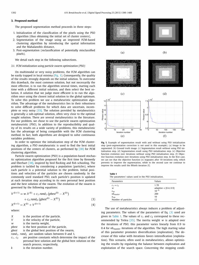
Fig. 1. Example of segmentation result with and without using PSO initializationstep (post-segmentation correction is not used in this example). (a) Image to besegmented. (b) Ground truth image. (c) Segmentation result without using PSO ini-tialization step. (d) Segmentation result using PSO initialization step. (e) Objectivefunction evolution over iterations without using PSO initialization step. (f) Objec-tive function evolution over iterations using PSO initialization step. In the first case,we can see that the objective function (e) stagnates after 10 iterations only, whichprevents to improve the segmentation, while in the second case we continue toimprove the results until the fiftieth iteration (f).

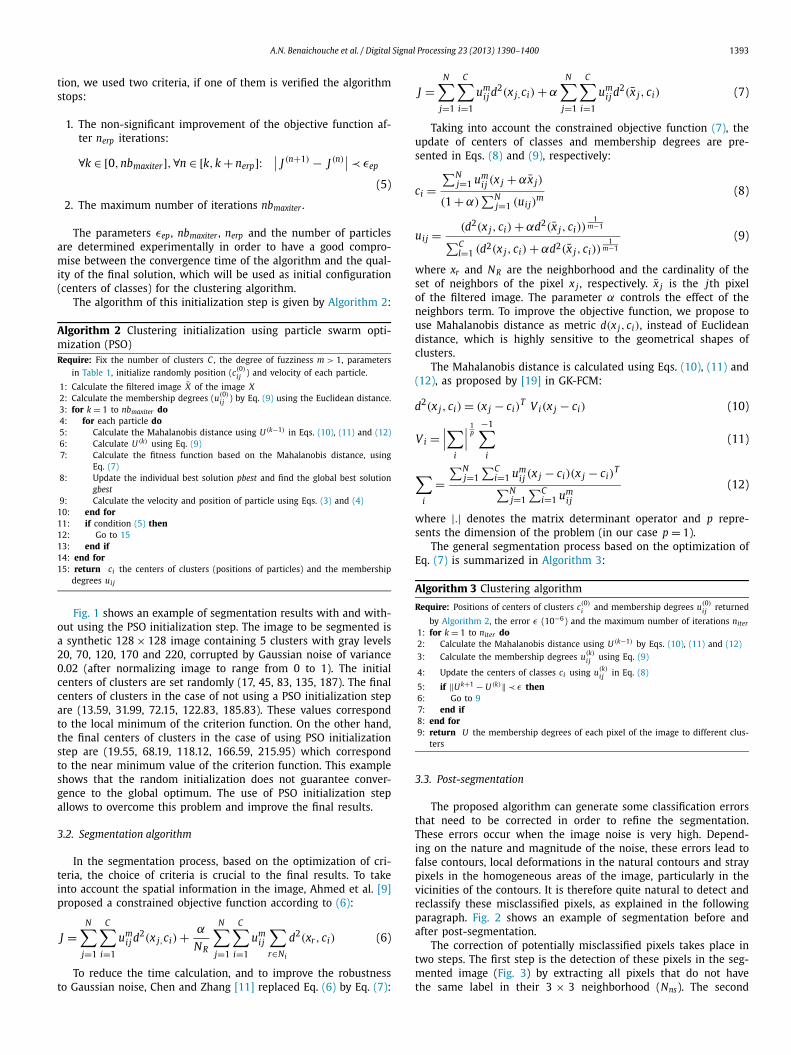
Table 1The parameters’ values used in the PSO initialization.

Parameters Values

c1 = c2 1.70w adaptive $ [0.4,0.9]!ep 10'6

nbmaxiter 200nerp 10Number of particles 12

The use of metaheuristics always induces a problem of adjust-ing parameters. The values of the parameters of Eq. (3) used aregiven in Table 1. The values of c1 and c2 correspond to these rec-ommended by Trelea [35]. The inertia weight w is adapted overthe iterations of PSO; this parameter varies linearly from 0.9 to0.4 for nbmaxiter iterations of the algorithm. The high starting valueof this parameter promotes diversification (exploration). The de-crease of this value with iterations favors intensification (exploita-tion). This scenario, often used in metaheuristics, allows optimiz-ing the results by regulating the balance between exploration andexploitation of the search space. Concerning the stopping condi-

A.N. Benaichouche et al. / Digital Signal Processing 23 (2013) 1390–1400 1393

tion, we used two criteria, if one of them is verified the algorithmstops:

1. The non-significant improvement of the objective function af-ter nerp iterations:

#k $ [0,nbmaxiter],#n $ [k,k + nerp]:%% J (n+1) ' J (n)

%% ) !ep

(5)

2. The maximum number of iterations nbmaxiter .

The parameters !ep , nbmaxiter , nerp and the number of particlesare determined experimentally in order to have a good compro-mise between the convergence time of the algorithm and the qual-ity of the final solution, which will be used as initial configuration(centers of classes) for the clustering algorithm.

The algorithm of this initialization step is given by Algorithm 2:

Algorithm 2 Clustering initialization using particle swarm opti-mization (PSO)Require: Fix the number of clusters C , the degree of fuzziness m > 1, parameters

in Table 1, initialize randomly position (c(0)i j ) and velocity of each particle.

1: Calculate the filtered image X̄ of the image X2: Calculate the membership degrees (u(0)

i j ) by Eq. (9) using the Euclidean distance.3: for k = 1 to nbmaxiter do4: for each particle do5: Calculate the Mahalanobis distance using U (k'1) in Eqs. (10), (11) and (12)6: Calculate U (k) using Eq. (9)7: Calculate the fitness function based on the Mahalanobis distance, using

Eq. (7)8: Update the individual best solution pbest and find the global best solution

gbest9: Calculate the velocity and position of particle using Eqs. (3) and (4)

10: end for11: if condition (5) then12: Go to 1513: end if14: end for15: return ci the centers of clusters (positions of particles) and the membership

degrees uij

Fig. 1 shows an example of segmentation results with and with-out using the PSO initialization step. The image to be segmented isa synthetic 128 " 128 image containing 5 clusters with gray levels20, 70, 120, 170 and 220, corrupted by Gaussian noise of variance0.02 (after normalizing image to range from 0 to 1). The initialcenters of clusters are set randomly (17, 45, 83, 135, 187). The finalcenters of clusters in the case of not using a PSO initialization stepare (13.59, 31.99, 72.15, 122.83, 185.83). These values correspondto the local minimum of the criterion function. On the other hand,the final centers of clusters in the case of using PSO initializationstep are (19.55, 68.19, 118.12, 166.59, 215.95) which correspondto the near minimum value of the criterion function. This exampleshows that the random initialization does not guarantee conver-gence to the global optimum. The use of PSO initialization stepallows to overcome this problem and improve the final results.

3.2. Segmentation algorithm

In the segmentation process, based on the optimization of cri-teria, the choice of criteria is crucial to the final results. To takeinto account the spatial information in the image, Ahmed et al. [9]proposed a constrained objective function according to (6):

J =N!

j=1

C!

i=1

umij d2(x j,ci) + "

NR

N!

j=1

C!

i=1

umij

!

r$Ni

d2(xr, ci) (6)

To reduce the time calculation, and to improve the robustnessto Gaussian noise, Chen and Zhang [11] replaced Eq. (6) by Eq. (7):

J =N!

j=1

C!

i=1

umij d2(x j,ci) + "

N!

j=1

C!

i=1

umij d2(x̄ j, ci) (7)

Taking into account the constrained objective function (7), theupdate of centers of classes and membership degrees are pre-sented in Eqs. (8) and (9), respectively:

ci ="N

j=1 umij (x j + "x̄ j)

(1 + ")"N

j=1 (uij)m

(8)

uij = (d2(x j, ci) + "d2(x̄ j, ci))1

m'1

"Cl=1 (d2(x j, ci) + "d2(x̄ j, ci))

1m'1

(9)

where xr and NR are the neighborhood and the cardinality of theset of neighbors of the pixel x j , respectively. x̄ j is the jth pixelof the filtered image. The parameter " controls the effect of theneighbors term. To improve the objective function, we propose touse Mahalanobis distance as metric d(x j, ci), instead of Euclideandistance, which is highly sensitive to the geometrical shapes ofclusters.

The Mahalanobis distance is calculated using Eqs. (10), (11) and(12), as proposed by [19] in GK-FCM:

d2(x j, ci) = (x j ' ci)T V i(x j ' ci) (10)

V i =%%%!

i

%%%1p

'1!

i

(11)

!

i

="N

j=1"C

i=1 umij (x j ' ci)(x j ' ci)

T

"Nj=1

"Ci=1 um

ij

(12)

where |.| denotes the matrix determinant operator and p repre-sents the dimension of the problem (in our case p = 1).

The general segmentation process based on the optimization ofEq. (7) is summarized in Algorithm 3:

Algorithm 3 Clustering algorithm

Require: Positions of centers of clusters c(0)i and membership degrees u(0)

i j returned

by Algorithm 2, the error ! (10'6) and the maximum number of iterations niter1: for k = 1 to niter do2: Calculate the Mahalanobis distance using U (k'1) by Eqs. (10), (11) and (12)3: Calculate the membership degrees u(k)

i j using Eq. (9)

4: Update the centers of classes ci using u(k)i j in Eq. (8)

5: if (U k+1 ' U (k)( ) ! then6: Go to 97: end if8: end for9: return U the membership degrees of each pixel of the image to different clus-

ters

3.3. Post-segmentation

The proposed algorithm can generate some classification errorsthat need to be corrected in order to refine the segmentation.These errors occur when the image noise is very high. Depend-ing on the nature and magnitude of the noise, these errors lead tofalse contours, local deformations in the natural contours and straypixels in the homogeneous areas of the image, particularly in thevicinities of the contours. It is therefore quite natural to detect andreclassify these misclassified pixels, as explained in the followingparagraph. Fig. 2 shows an example of segmentation before andafter post-segmentation.

The correction of potentially misclassified pixels takes place intwo steps. The first step is the detection of these pixels in the seg-mented image (Fig. 3) by extracting all pixels that do not havethe same label in their 3 " 3 neighborhood (Nns). The second

1394 A.N. Benaichouche et al. / Digital Signal Processing 23 (2013) 1390–1400

Fig. 2. Example of segmentation before and after post-segmentation. (a) Noised im-ages to be segmented. (b) Ground truth images. (c) Segmentation results beforepost-segmentation. (d) Segmentation results after post-segmentation.

step is the reclassification of these extracted pixels by minimiz-ing homogeneous criterion (13), using local information in a 5 " 5neighborhood (Nrl) of each extracted pixel in the original image.Note that each extracted pixel can be reassigned only to a clusterof its Nns neighborhood. The cluster of reallocation can change orbe the same as before. Indeed, this detection method can extractall misclassified pixels, but also some correctly classified pixels inthe neighborhood. It is therefore natural to reallocate the correctlyclassified pixels to their original cluster and all misclassified pixelsto the most appropriate cluster.

Fig. 3. Reclustering of the potentially misclassified pixels. (a) Segmentation resultsbefore post-segmentation. (b) Potentially misclassified pixels detected. (c) The realmisclassified pixels before post-segmentation (difference between (b) and (c) inFig. 2). (d) The real misclassified pixels after post-segmentation (difference between(b) and (d) in Fig. 2).

J i ="# (i)

j + (xi ' u(i)j (

$N j+

N pi!

k=1, k *= j

# (i)k (13)

where:

Npi is the number of different labels present in Nrl neighbor-hood of the pixel i,

N j is the number of pixels belonging to the cluster j in Nrlneighborhood of the pixel i,

A.N. Benaichouche et al. / Digital Signal Processing 23 (2013) 1390–1400 1395

xi is the extracted pixel to be reclassified,u(i)

j is the local mean of the class j in Nrl neighborhood,

# (i)j is the local variance of the cluster j in the Nrl neighbor-

hood of the pixel xi after its reallocation to this cluster,# (i)

k is the local variance of the cluster k in the Nrl neighbor-hood of the pixel xi ,

" is a parameter which allows to adjust the impact of thelocal variance on the reallocation of pixels. Its value isdetermined experimentally and set to 0.65,

$ is a fixed parameter which determines the impact of thenumber of pixels belonging to the cluster j. This param-eter is set to 1/Nrl such that $N j represents the pro-portion of the cluster j in the local neighborhood of thepixel to be reclassified.

Thus, the extracted pixel xi is reallocated to the class j thatminimizes the objective function J i ( j = argmin( J i)), see Algo-rithm 4:

Algorithm 4 Post-segmentationStep 1: Extraction of potentially misclassified pixels (xl )1: l & 12: for all pixels xi of the image do3: if (label(xi) *= label(x j $ Nns)) then4: xl & xi5: for all clusters m in Nrl neighborhood of the pixel xl do6: Calculate the local variance # (l)

m

7: Calculate the local mean µ(l)m

8: end for9: l & l + 1

10: end if11: end for12: return xl , # (l)

m and µ(l)m

Step 2: Reclassification of the extracted pixels1: for all extracted pixels xi do2: for j = 1 to Npi do3: Calculate the objective function J i using Eq. (13)4: Find j = argmin( J i)

5: Assign the pixel xi to the cluster j6: end for7: end for

4. Experimental results

In this section, the experimental results of the proposedmethod are described, and compared with six well-known FCM-based methods of the literature: FCM, FCM-S1, FCM-S2, EnFCM,FGFCM and FLICM. Two types of images were used: syntheticimages with different numbers of clusters and corrupted with dif-ferent levels and types of noises, and simulated MRI brain imagesdownloaded from Brainweb [36]. In order to compare objectivelythe different algorithms, the optimal segmentation accuracy (SA) isused. SA is defined as the sum of the correctly classified pixels di-vided by the sum of the total number of pixels of the test image(Eq. (14)):

SA =c!

i=1

card(Ai + Ci)"cj=1 card(C j)

(14)

where c is the number of clusters, Ai is the set of pixels belongingto the ith cluster found by the algorithm, Ci is the set of the ithcluster in the ground truth segmented image.

The algorithms were implemented in Matlab version 7 and runon a 2.60 GHz Pentium(R) Dual-Core CPU, under Microsoft Win-dows XP pro Operating system.

The values of the parameters of the algorithms cited above arethose chosen by [15]. The values of the parameters of our methodwere already given in the previous subsections.

The results of the concurrent FCM algorithms strongly dependon the initial solution (starting solution). To reduce the influenceof the initial solution, we run each of them 10 times, starting eachtime from a random solution. The results presented are the averageof these 10 executions.

4.1. Results on synthetic images

To compare the robustness of the different algorithms citedabove, we apply them firstly to 256 " 256 synthetic images con-taining 2, 3, 4 or 5 clusters and corrupted with Gaussian, uniformor salt & pepper noises. The levels of these different types of noisesare 10%, 15%, 20% and 25% for images containing 2 or 3 clusters,and 3%, 5%, 8% and 10% for those containing 4 or 5 clusters. Figs. 4and 5 illustrate examples of the segmentation results of syntheticimages containing 5 clusters corrupted with 3% Gaussian noise, 3%uniform noise and 10% salt and pepper noise (Fig. 4(b)).

Visually, FCM-S1 (Fig. 4(d)) and FLICM (Fig. 5(c)) methods re-move most of the Gaussian and uniform noise, but give poorresults in the case of salt and pepper noise. FCM-S2 method(Fig. 4(e)) removes some of salt and pepper noise, but the result isnot satisfactory. On the other hand, the proposed method removesthe most added noise in the three cases, Gaussian noise, uniformnoise and salt and pepper noise and gives quite satisfactory results,which are verified by the segmentation accuracy (SA) in Tables 2and 3.

Tables 2 and 3 give the average segmentation accuracy (SA) ofthe seven algorithms according to the noise type and the num-ber of clusters, respectively. These tables show that the proposedmethod performs clearly better than the other methods, and ismore robust towards type and level of noises and number of clus-ters. Fig. 6 shows the average SA of the seven algorithms on theentire synthetic images database. We can see in this figure thatthe proposed method gives better results than all other FCM-basedmethods.

4.2. Results on simulated MRI images

The ground truth of segmentation for the real MRI images isoften not available, making the quantitative evaluation of the seg-mentation performance impossible. Otherwise, Brainweb providesa Simulated Brain Database (SBD) which contains a set of realisticMRI data volumes produced by an MRI simulator. The availabilityof the ground truth of segmentation enables us to evaluate quanti-tatively the segmentation performances of the different algorithms.The database used contains the 91th brain region slice in the axialplane generated with T1 modality, 1 mm slice thickness. This slicewas noised with 3%, 7% and 9%, the intensity non-uniformity pa-rameter was set to 0%, 20% and 40% for each noise level. These im-ages were segmented on four clusters: background, cerebral spinalfluid (CSF), gray matter and white matter using the seven algo-rithms. Figs. 7 and 8 show the segmentation results for an imagecontaining 7% of noise and 20% intensity of non-uniformity pa-rameter, the background was neglected from the viewing results.Table 4 gives the average of the segmentation accuracy (SA) of theseven algorithms on the database for each cluster and their globalaverage. The evaluation analysis shows that the proposed methodgives better results than the methods used for comparison, for thisdatabase too.

5. Conclusion

In this paper, we presented an improvement of the FCM algo-rithm applied to image segmentation by overcoming its drawbacks.

1396 A.N. Benaichouche et al. / Digital Signal Processing 23 (2013) 1390–1400

Fig. 4. Examples of segmentation on synthetic images.

The first improvement lies in the initialization step of the algo-rithm by using the PSO metaheuristic in order to overcome thetrapping of the solution in local minima. The second one con-cerns the classification criterion which was improved by introduc-ing the local information and the Mahalanobis distance, so thatthe segmentation will be more robust against noise and will takeinto account the geometric shape of the clusters. Finally, a post-segmentation stage was used to refine the results by detectingand reclustering the potentially misclassified pixels, by using anew local criterion optimized by a greedy algorithm. The proposedmethod was tested and compared to the six most used FCM-based

algorithms of the literature. Two kinds of images were used inthe performance evaluation: synthetic images containing differentnumbers of clusters, types and levels of noises and simulated brainMRI images containing different levels of noise and intensity ofnon-uniformity parameters. For the two test databases, the experi-mental results show that the proposed method gives better resultsand is more robust against types of noise and numbers of clus-ters than the other FCM-based methods. Nonetheless, in the pres-ence of high noise, some pixels located at the boundaries betweentwo adjacent regions are still misclassified. To reduce the num-ber of these misclassified pixels, several approaches are possible.

A.N. Benaichouche et al. / Digital Signal Processing 23 (2013) 1390–1400 1397

Fig. 5. Examples of segmentation on synthetic images (next results).

Fig. 6. Global average SA on synthetic images database.

1398 A.N. Benaichouche et al. / Digital Signal Processing 23 (2013) 1390–1400

Table 2Average segmentation accuracy (SA%) of the seven algorithms according to the number of clusters and the level of noise.

FCM FCM_S1 FCM_S2 EnFCM FGFCM FLICM IFCMS

Gaussian 47.48 85.16 78.68 78.07 88.92 91.99 93.11Uniform 42.40 83.06 74.30 76.31 76.31 94.49 95.17Salt & pepper 75.81 81.02 90.05 79.69 72.50 58.39 91.69

Table 3Average segmentation accuracy (SA%) of the seven algorithms according to the level and the type of noise.

FCM FCM_S1 FCM_S2 EnFCM FGFCM FLICM IFCMS

2 classes 90.66 96.91 99.90 94.98 94.99 96.27 99.833 classes 65.66 80.32 77.80 83.98 84.44 82.48 95.644 classes 38.18 79.55 75.68 78.68 77.81 75.21 93.135 classes 26.42 75.53 70.64 54.47 66.73 72.54 84.68

Fig. 7. Examples of segmentation on simulated brain MRI image.

A.N. Benaichouche et al. / Digital Signal Processing 23 (2013) 1390–1400 1399

Fig. 8. Examples of segmentation on simulated brain MRI image (next results).

Table 4Average of the segmentation accuracy (SA%) of the seven algorithms on the MRI-database for each cluster and their global average.

FCM FCM_S1 FCM_S2 EnFCM FGFCM FLICM IFCMS

CSF 93.93 93.17 93.25 92.44 91.64 90.52 94.50Gray matter 89.66 90.61 92.71 85.14 85.27 92.55 93.81White matter 88.81 92.46 92.75 90.92 90.97 91.77 93.10

Average 90.80 92.08 92.90 89.50 89.29 91.61 93.80

Particularly, we plan to use a metaheuristic optimization algorithmin the post-segmentation stage instead of a greedy algorithm, soas not to be trapped in a local optimum, and to apply a multi-objective optimization approach, in order to integrate and mergethe advantages of two or multiple criteria.

References

[1] M. Christ, R.M.S. Parvathi, Magnetic resonance brain image segmentation, In-tern. J. VLSI Design Commun. Syst. 3 (2012) 121–133.

[2] V. Dey, Y. Zhang, M. Zhong, A review on image segmentation techniques withremote sensing perspective, in: W. Wagner, B. Székely (Eds.), ISPRS TC VII Sym-posium – 100 Years ISPRS, vol. XXXVIII, Vienna, Austria, 2011, pp. 31–42.

[3] K.C. Ciesielski, J.K. Udupa, Region-based segmentation: Fuzzy connectedness,graph cut and related algorithms, in: T.M. Deserno (Ed.), Biomedical ImageProcessing, Biological and Medical Physics, Biomedical Engineering, Springer,Berlin, Heidelberg, 2011, pp. 251–278.

[4] A. Nakib, H. Oulhadj, P. Siarry, A thresholding method based on two-dimensional fractional differentiation, Image Vis. Comput. 27 (2009)1343–1357.

[5] G. Papari, N. Petkov, Edge and line oriented contour detection: State of the art,Image Vis. Comput. 29 (2011) 79–103.

[6] L. Zadeh, Fuzzy sets, Inform. Control 8 (1965) 338–353.[7] J.C. Bezdek, Pattern Recognition with Fuzzy Objective Function Algorithms,

Kluwer Academic Publishers, Norwell, MA, USA, 1981.[8] D.L. Pham, J.L. Prince, An adaptive fuzzy c-means algorithm for image segmen-

tation in the presence of intensity inhomogeneities, Pattern Recogn. Lett. 20(1999) 57–68.

[9] M. Ahmed, S. Yamany, N. Mohamed, A. Farag, T. Moriarty, A modified fuzzyc-means algorithm for bias field estimation and segmentation of MRI data, IEEETrans. Med. Imag. 21 (2002) 193–199.

[10] D. Pham, Fuzzy clustering with spatial constraints, in: Proceedings of the In-ternational Conference on Image Processing, vol. 2, New York, USA, 2002,pp. II-65–II-68.

[11] S. Chen, D. Zhang, Robust image segmentation using FCM with spatial con-straints based on new kernel-induced distance measure, IEEE Trans. Syst. ManCybern., Part B, Cybern. 34 (2004) 1907–1916.

[12] L. Szilagyi, Z. Benyo, S. Szilagyi, H. Adam, MR brain image segmentation us-ing an enhanced fuzzy C-means algorithm, in: Proceedings of the 25th AnnualInternational Conference of the IEEE, vol. 1, Cancun, Mexico, Engineering inMedicine and Biology Society, 2003, pp. 724–726.

1400 A.N. Benaichouche et al. / Digital Signal Processing 23 (2013) 1390–1400

[13] J. Kang, W. Zhang, Fingerprint image segmentation using modified fuzzyc-means algorithm, in: 3rd International Conference on Bioinformatics andBiomedical Engineering, ICBBE 2009, Beijing, P.R. China, 2009, pp. 1–4.

[14] W. Cai, S. Chen, D. Zhang, Fast and robust fuzzy c-means clustering algorithmsincorporating local information for image segmentation, Pattern Recogn. 40(2007) 825–838.

[15] S. Krinidis, V. Chatzis, A robust fuzzy local information c-means clustering al-gorithm, IEEE Trans. Image Process. 19 (2010) 1328–1337.

[16] R. Krishnapuram, J. Kim, A note on the Gustafson–Kessel and adaptive fuzzyclustering algorithms, IEEE Trans. Fuzzy Syst. 7 (1999) 453–461.

[17] D.E. Gustafson, W.C. Kessel, Fuzzy clustering with a fuzzy covariance matrix,in: IEEE Conference on Decision and Control including the 17th Symposium onAdaptive Processes, vol. 17, San Diego, CA, USA, 1978, pp. 761–766.

[18] I. Gath, A. Geva, Unsupervised optimal fuzzy clustering, IEEE Trans. PatternAnal. Mach. Intell. 11 (1989) 773–780.

[19] H.-C. Liu, B.-C. Jeng, J.-M. Yih, Y.-K. Yu, Fuzzy C-means algorithm based on stan-dard mahalanobis distances, in: Proceedings of the International Symposiumon Information Processing, ISIP’09, Huangshan, P.R. China, 2009, pp. 422–427.

[20] S.R. Kannan, R. Devi, S. Ramathilagam, K. Takezawa, Effective FCM noise clus-tering algorithms in medical images, Comput. Biol. Med. 43 (2) (2013) 73–83.

[21] U. Maulik, S. Bandyopadhyay, Genetic algorithm-based clustering technique,Pattern Recogn. 33 (2000) 1455–1465.

[22] M.K. Ng, J.C. Wong, Clustering categorical data sets using tabu search tech-niques, Pattern Recogn. 35 (2002) 2783–2790.

[23] T. Niknam, B. Amiri, An e!cient hybrid approach based on PSO, ACO and k-means for cluster analysis, Applied Soft Computing 10 (2010) 183–197.

[24] N. Taher, A. Babak, O. Javad, A. Ali, An e!cient hybrid evolutionary optimiza-tion algorithm based on PSO and SA for clustering, J. Zhejiang Univ. Sci. Ed. 10(2009) 512–519.

[25] S. Das, A. Abraham, A. Konar, Metaheuristic Clustering, Stud. Comput. Intell.,vol. 178, Springer, 2009.

[26] O. Alia, M. Al-Betar, R. Mandava, A. Khader, Data clustering using harmonysearch algorithm, in: B. Panigrahi, P. Suganthan, S. Das, S. Satapathy (Eds.),Swarm, Evolutionary, and Memetic Computing, in: Lecture Notes in Comput.Sci., vol. 7077, Springer, Berlin, Heidelberg, 2011, pp. 79–88.

[27] K.S. Al-Sultan, C.A. Fedjki, A tabu search-based algorithm for the fuzzy cluster-ing problem, Pattern Recogn. 30 (1997) 2023–2030.

[28] H. Izakian, A. Abraham, Fuzzy c-means and fuzzy swarm for fuzzy clusteringproblem, Expert Syst. Appl. 38 (2011) 1835–1838.

[29] W. Pang, K. Wang, C. Zhou, L. Dong, Fuzzy discrete particle swarm optimizationfor solving traveling Salesman problem, in: Proceedings of Fourth InternationalConference on Computer and Information Technology, CIT ’04, IEEE ComputerSociety, Washington, DC, USA, 2004, pp. 796–800.

[30] Y. Zhang, D. Huang, M. Ji, F. Xie, Image segmentation using PSO and PCM withMahalanobis distance, Expert Syst. Appl. 38 (2011) 9036–9040.

[31] R. Krishnapuram, J. Keller, A possibilistic approach to clustering, IEEE Trans.Fuzzy Syst. 1 (1993) 98–110.

[32] C. Bong, M. Rajeswari, Multiobjective clustering with metaheuristic: currenttrends and methods in image segmentation, IET Image Process. 6 (2012) 1–10.

[33] J. Dréo, A. Pétrowski, P. Siarry, E. Taillard, Metaheuristics for Hard Optimization,Springer, 2005.

[34] J. Kennedy, R. Eberhart, Particle swarm optimization, in: Proceedings IEEEInternational Conference on Neural Networks, vol. 4, Perth, Australia, 1995,pp. 1942–1948.

[35] I.C. Trelea, The particle swarm optimization algorithm: convergence analysisand parameter selection, Inform. Process. Lett. 85 (2003) 317–325.

[36] http://www.bic.mni.mcgill.ca/brainweb/, 2012.

Ahmed Nasreddine Benaichouche was born in Algeria in 1988. Hereceived the engineering degree in electronics and automatics from theNational Polytechnic School of Algiers, in 2010. He received his DEA de-gree in signal and image processing from the University Paris 6, in 2011and is currently a PhD student in the University Paris-Est Créteil, since2011. His research interests are in the areas of optimization, image pro-cessing and machine learning.

Hamouche Oulhadj was born in Algeria in 1956. He received hisdegree in Electrical and Electronics Engineering from the PolytechnicSchool of Algiers, then the DEA and the PhD degree in Biomedical En-gineering from the University Paris 12, respectively, in 1985 and 1990.He is presently an Associate Professor at the same university, currentlyrenowned University Paris-Est Créteil. His research interests are focusedon image processing and optimization.

Patrick Siarry was born in France in 1952. He received the PhD de-gree from the University Paris 6, in 1986, and the Doctorate of Sciences(Habilitation) from the University Paris 11, in 1994. He was first involvedin the development of analog and digital models of nuclear power plantsat Electricité de France (E.D.F.). Since 1995 he is a Professor in automaticsand informatics. His main research interests are computer-aided design ofelectronic circuits, and the applications of new stochastic global optimiza-tion heuristics to various engineering fields. He is also interested in thefitting of process models to experimental data, the learning of fuzzy rulebases, and of neural networks.