tug-of-war and the infinity laplacian

JOURNAL OF THEAMERICAN MATHEMATICAL SOCIETYVolume 22, Number 1, January 2009, Pages 167–210S 0894-0347(08)00606-1Article electronically published on July 28, 2008

TUG-OF-WAR AND THE INFINITY LAPLACIAN

YUVAL PERES, ODED SCHRAMM, SCOTT SHEFFIELD, AND DAVID B. WILSON

1. Introduction and preliminaries

1.1. Overview. We consider a class of zero-sum two-player stochastic games calledtug-of-war and use them to prove that every bounded real-valued Lipschitz func-tion F on a subset Y of a length space X admits a unique absolutely minimal(AM) extension to X, i.e., a unique Lipschitz extension u : X → R for whichLipUu = Lip∂Uu for all open U ⊂ X � Y . We present an example that showsthis is not generally true when F is merely Lipschitz and positive. (Recall that ametric space (X, d) is a length space if for all x, y ∈ X, the distance d(x, y) is theinfimum of the lengths of continuous paths in X that connect x to y. Length spacesare more general than geodesic spaces, where the infima need to be achieved.)

When X is the closure of a bounded domain U ⊂ Rn and Y is its boundary, a

Lipschitz extension u of F is AM if and only it is infinity harmonic in the interiorof X � Y ; i.e., it is a viscosity solution (defined below) to ∆∞u = 0, where ∆∞is the so-called infinity Laplacian

(1.1) ∆∞u = |∇u|−2∑i,j

uxiuxixj

uxj

(informally, this is the second derivative of u in the direction of the gradient ofu). Aronsson proved this equivalence for smooth u in 1967, and Jensen proved thegeneral statement in 1993 [1, 13]. Our analysis of tug-of-war also shows that in thissetting ∆∞u = g has a unique viscosity solution (extending F ) when g : U → R iscontinuous and inf g > 0 or sup g < 0, but not necessarily when g assumes values ofboth signs. We note that in the study of the homogenous equation ∆∞u = 0, thenormalizing factor |∇u|−2 in (1.1) is sometimes omitted; however, it is important toinclude it in the non-homogenous equation. Observe that with the normalization,∆∞ coincides with the ordinary Laplacian ∆ in the one-dimensional case.

Unlike the ordinary Laplacian or the p-Laplacian for p < ∞, the infinity Lapla-cian can be defined on any length space with no additional structure (such as ameasure or a canonical Markov semigroup)—that is, we will see that viscosity so-lutions to ∆∞u = g are well defined in this generality. We will establish the abovestated uniqueness of solutions u to ∆∞u = g in the setting of length spaces.

Originally, we were motivated not by the infinity Laplacian but by random turnHex [22] and its generalizations, which led us to consider the tug-of-war game. As

Received by the editors July 11, 2006.2000 Mathematics Subject Classification. Primary 91A15, 91A24, 35J70, 54E35, 49N70.Key words and phrases. Infinity Laplacian, absolutely minimal Lipschitz extension, tug-of-war.Research of the first and third authors was supported in part by NSF grants DMS-0244479

and DMS-0104073.

c©2008 by the authors. This paper or any part thereof may be reproduced for non-commercial purposes.

167

License or copyright restrictions may apply to redistribution; see https://www.ams.org/journal-terms-of-use

168 Y. PERES, O. SCHRAMM, S. SHEFFIELD, AND D. B. WILSON

we later learned, tug-of-war games have been considered by Lazarus, Loeb, Proppand Ullman in [16] (see also [15]).

Tug-of-war on a metric space is very natural and conceivably applicable (likedifferential game theory) to economic and political modeling.

The intuition provided by thinking of strategies for tug-of-war yields new resultseven in the classical setting of domains in Rn. For instance, in Section 4 we showthat if u is infinity harmonic in the unit disk and its boundary values are in [0, 1]and supported on a δ-neighborhood of the ternary Cantor set on the unit circle,then u(0) < δβ for some β > 0.

Before precisely stating our main results, we need several definitions.

1.2. Random turn games and values. We consider two-player, zero-sumrandom-turn games, which are defined by the following parameters: a set Xof states of the game, two directed transition graphs EI, EII with vertex set X,a non-empty set Y ⊂ X of terminal states (a.k.a. absorbing states), a termi-nal payoff function F : Y → R, a running payoff function f : X � Y → R,and an initial state x0 ∈ X.

The game play is as follows: a token is initially placed at position x0. At the kth

step of the game, a fair coin is tossed, and the player who wins the toss may movethe token to any xk for which (xk−1, xk) is a directed edge in her transition graph.The game ends the first time xk ∈ Y , and player I’s payoff is F (xk) +

∑k−1i=0 f(xi).

Player I seeks to maximize this payoff, and since the game is zero-sum, player IIseeks to minimize it.

We will use the term tug-of-war (on the graph with edges E) to describethe game in which E := EI = EII (i.e., players have identical move options) and Eis undirected (i.e., all moves are reversible). Generally, our results pertain only tothe undirected setting. Occasionally, we will also mention some counterexamplesshowing that the corresponding results do not hold in the directed case.

In the most conventional version of tug-of-war on a graph, Y is a union of “targetsets” Y I and Y II, there is no running payoff (f = 0), and F is identically 1 on Y I andidentically 0 on Y II. Players then try to “tug” the game token to their respectivetargets (and away from their opponent’s targets), and the game ends when a targetis reached.

A strategy for a player is a way of choosing the player’s next move as a functionof all previously played moves and all previous coin tosses. It is a map from theset of partially played games to moves (or in the case of a random strategy, aprobability distribution on moves). Normally, one would think of a good strategyas being Markovian, i.e., as a map from the current state to the next move, but itis useful to allow more general strategies that take into account the history.

Given two strategies SI,SII, let F−(SI,SII) and F+(SI,SII) be the expected totalpayoff (including the running payoffs received) at the termination of the game, ifthe game terminates with probability one and this expectation exists in [−∞,∞];otherwise, let F−(SI,SII) = −∞ and F+(SI,SII) = +∞.

The value of the game for player I is defined as supSIinfSII F−(SI,SII). The

value for player II is infSII supSIF+(SI,SII). We use the expressions uI(x) and

uII(x) to denote the values for players I and II, respectively, as a function of thestarting state x of the game.

Note that if player I cannot force the game to end almost surely, then uI = −∞,and if player II cannot force the game to end almost surely, then uII = ∞. Clearly,


TUG-OF-WAR AND THE INFINITY LAPLACIAN 169

uI(x) ≤ uII(x). When uI(x) = uII(x), we say that the game has a value, given byu(x) := uI(x) = uII(x).

Our definition of value for player I penalizes player I severely for not forcing thegame to terminate with probability one, awarding −∞ in this case.

(As an alternative definition, one could define F−, and hence player I’s value, byassigning payoffs to all of the non-terminating sequences x0, x1, x2, . . .. If the payofffunction for the non-terminating games is a zero-sum Borel-measurable function ofthe infinite sequence, then player I’s value is equal to player II’s value in greatgenerality [17]; see also [20] for more on stochastic games. The existence of a valueby our strong definition implies the existence and equality of the values defined bythese alternative definitions.)

Considering the two possibilities for the first coin toss yields the following lemma,a variant of which appears in [16].

Lemma 1.1. The function u = uI satisfies the equation

(1.2) u(x) =12

(sup

y:(x,y)∈E1

u(y) + infy:(x,y)∈E2

u(y)

)+ f(x)

for every non-terminal state x ∈ X�Y for which the right-hand side is well defined,and uI(x) = −∞ when the right-hand side is of the form 1

2 (∞+(−∞))+f(x). Theanalogous statement holds for uII, except that uII(x) = +∞ when the right-handside of (1.2) is of the form 1

2 (∞ + (−∞)) + f(x).

When E = E1 = E2, the operator

∆∞u(x) := supy:(x,y)∈E

u(y) + infy:(x,y)∈E

u(y) − 2u(x)

is called the (discrete) infinity Laplacian. A function u is infinity harmonicif (1.2) holds and f(x) = 0 at all non-terminal x ∈ X � Y . When u is finite, thisis equivalent to ∆∞u = 0. However, it will be convenient to adopt the conventionthat u is infinity harmonic at x if u(x) = +∞ (resp. −∞) and the right-hand sidein (1.2) is also +∞ (resp. −∞). Similarly, it will be convenient to say “u is asolution to ∆∞u = −2 f” at x if u(x) = +∞ (resp. −∞) and the right-hand sidein (1.2) is also +∞ (resp. −∞).

In a tug-of-war game, it is natural to guess that the value u = uI = uII existsand is the unique solution to

∆∞u(x) = −2f,

and also that (at least when E is locally finite) player I’s optimal strategy will be toalways move to the vertex that maximizes u(x) and that player II’s optimal strategywill be to always move to the vertex that minimizes u(x). This is easy to prove whenE is undirected and finite and f is everywhere positive or everywhere negative.Subtleties arise in more general cases (X infinite, E directed, F unbounded, fhaving values of both signs, etc.).

Our first theorem addresses the question of the existence of a value.

Theorem 1.2. A tug-of-war game with parameters X, E, Y, F, f has a value when-ever the following hold:

(1) Either f = 0 everywhere or inf f > 0.(2) inf F > −∞.(3) E is undirected.



Counterexamples exist when any one of the three criteria is removed. In Section 5(a section devoted to counterexamples) we give an example of a tug-of-war gamewithout a value, where E is undirected, F = 0, and the running payoff satisfiesf > 0 but inf f = 0.

The case where f = 0, F is bounded, and (X, E) is locally finite was provedearlier in [15]. That paper discusses an (essentially non-random) game in whichthe two players bid for the right to choose the next move. That game, called theRichman game, has the same value as tug-of-war with f = 0, where F takes thevalues 0 and 1. Additionally, a simple and efficient algorithm for calculating thevalue when f = 0 and (X, E) is finite is presented there.

1.3. Tug-of-war on a metric space. Now consider the special case where (X, d)is a metric space, Y ⊂ X, and Lipschitz functions F : Y → R and f : X � Y → R

are given. Let Eε be the edge-set in which x ∼ y if and only if d(x, y) < ε, and letuε be the value (if it exists) of the game played on Eε with terminal payoff F andrunning payoff normalized to be ε2f .

In other words, uε(x) is the value of the following two-player zero-sum game,called ε-tug-of-war: fix x0 = x ∈ X � Y . At the kth turn, the players toss a coinand the winner chooses an xk with d(xk, xk−1) < ε. The game ends when xk ∈ Y ,and player I’s payoff is F (xk) + ε2

∑k−1i=0 f(xi).

When the limit u := limε→0 uε exists pointwise, we call u the continuum value(or just “value”) of the quintuple (X, d, Y, F, f). We define the continuum valuefor player I (or II) analogously.

The reader may wonder why we have chosen not to put an edge in Eε betweenx and y when d(x, y) = ε exactly. This choice has some technical implications.Specifically, we will compare the ε-game with the 2 ε-game. If x, z are such thatd(x, z) ≤ 2 ε, then in a length space it does not follow that there is a y suchthat d(x, y) ≤ ε and d(y, z) ≤ ε. However, it does follow if you replace the weakinequalities with strong inequalities throughout.

We prove the following:

Theorem 1.3. Suppose X is a length space, Y ⊂ X is non-empty, F : Y → R isbounded below and has an extension to a uniformly continuous function on X, andeither f : X � Y → R satisfies f = 0 or all three of the following hold: inf |f | >0, f is uniformly continuous, and X has finite diameter. Then the continuumvalue u exists and is a uniformly continuous function extending F . Furthermore,‖u− uε‖∞ → 0 as ε ↘ 0. If F is Lipschitz, then so is u. If F and f are Lipschitz,then ‖u − uε‖∞ = O(ε).

The above condition that F : Y → R extends to a uniformly continuous functionon X is equivalent to having F uniformly continuous on Y and “Lipschitz on largescales,” as we prove in Lemma 3.9 below.

We will see in Section 5.1 that this fails in general when f > 0 but inf f =0. When f assumes values of both signs, it fails even when X is a closed diskin R

2, Y is its boundary and F = 0. In Section 5.3 we show by means of anexample that in such circumstances it may happen that uε

I = uεII and moreover,

lim infε↘0 ‖uεI − uε

II‖∞ > 0.



1.4. Absolutely minimal Lipschitz extensions. Given a metric space (X, d),a subset Y ⊂ X and a function u : X → R, we write

LipY u = supx,y∈Y

|u(y) − u(x)|/d(x, y)

and Lipu = LipXu. Thus u is Lipschitz iff Lip u < ∞. Given F : Y → R, we saythat u : X → R is a minimal extension of F if LipXu = LipY F and u(y) = F (y)for all y ∈ Y .

It is well known that for any metric space X, any Lipschitz F on a subset Yof X admits a minimal extension. The largest and smallest minimal extensions(introduced by McShane [18] and Whitney [24] in the 1930’s) are respectively

infy∈Y

[F (y) + LipY F d(x, y)] and supy∈Y

[F (y) − LipY F d(x, y)] .

We say u is an absolutely minimal (AM) extension of F if Lip u < ∞ andLipUu = Lip∂Uu for every open set U ⊂ X � Y . We say that u is AM on U if it isdefined on U and is an AM extension of its restriction to ∂U . AM extensions werefirst introduced by Aronsson in 1967 [1] and have applications in engineering andimage processing (see [4] for a recent survey).

We prove the following:

Theorem 1.4. Let X be a length space and let F : Y → R be Lipschitz, where∅ = Y ⊂ X. If inf F > −∞, then the continuum value function u described inTheorem 1.3 (with f = 0) is an AM extension of F . If F is also bounded, then uis the unique AM extension of F .

We present in the counterexample section, Section 5, an example in which F isLipschitz, non-negative, and unbounded, and although the continuum value is anAM extension, it is not the only AM extension.

Prior to our work, the existence of AM extensions in the above settings wasknown only for separable length spaces [14] (see also [19]). The uniqueness inTheorem 1.4 was known only in the case that X is the closure of a bounded domainU ⊂ Rn and Y = ∂U . (To deduce this case from Theorem 1.4, one needs toreplace X by the smallest closed ball containing U , say.) Three uniqueness proofsin this setting have been published, by Jensen [13], by Barles and Busca [6], andby Aronsson, Crandall, and Juutinen [4]. The third proof generalizes from theEuclidean norm to uniformly convex norms.

Our proof applies to more general spaces because it invokes no outside theoremsfrom analysis (which assume existence of a local Euclidean geometry, a measure,a notion of twice differentiability, etc.), and relies only on the structure of X as alength space.

As noted in [4], AM extensions do not generally exist on metric spaces that arenot length spaces. (For example, if X is the L-shaped region {0} × [0, 1] ∪ [0, 1] ×{0} ⊂ R2 with the Euclidean metric, and Y = {(0, 1), (1, 0)}, then no non-constantF : Y → R has an AM extension. Indeed, suppose that u : X → R is an AMextension of F : Y → R. Let a := u(0, 0), b := u(0, 1) and c := u(1, 0). Then,considering U = {0} × (0, 1), it follows that u(0, s) = a + s (b − a). Likewise,u(s, 0) = a + s (c − a). Now taking Uε := {0} × [0, 1) ∪ [0, ε) × {0}, we see thatlimε↘0 LipUε

u = |b − a|. Hence |c − a| ≤ |b − a|. By symmetry, |c − a| = |b − a|.Since F is assumed to be non-constant, b = c, and hence c − a = a − b. Then∣∣u(0, s) − u(s, 0)

∣∣/(√2s

)=

√2 |b − a|, which contradicts limε↘0 LipUε

u = |b − a|.)



One property that makes length spaces special is the fact that the Lipschitz normis determined locally. More precisely, if W ⊂ X is closed, then either LipW u =Lip∂W u or for every δ > 0

sup{ |u(x) − u(y)|

d(x, y): x, y ∈ W, 0 < d(x, y) < δ

}= LipW u .

The definition of AM was inspired by the notion that if u is the “tautest possible”Lipschitz extension of F , it should be tautest possible on any open V ⊂ X � Y ,given the values of u on ∂V and ignoring the rest of the metric space. Withoutlocality, the rest of the metric space cannot be ignored (since long-distance effectsmay change the global Lipschitz constant), and the definition of AM is less natural.Another important property of length spaces is the fact that the graph distancemetric on Eε scaled by ε approximates the original metric, namely, it is within ε ofd(·, ·).

1.5. Infinity Laplacian on Rn. The continuum version of the infinity Laplacianis defined for C2 functions u on domains U ⊂ R

n by

∆∞u = |∇u|−2∑i,j

uxiuxixj

uxj.

This is the same as ηT Hη, where H is the Hessian of u and η = ∇u/|∇u|. Infor-mally, ∆∞u is the second derivative of u in the direction of the gradient of u. If∇u(x) = 0, then ∆∞u(x) is undefined; however, we adopt the convention that ifthe second derivative of u(x) happens to be the same in every direction (i.e., thematrix {uxixj

} is λ times the identity), then ∆∞u(x) = λ, which is the secondderivative in any direction. (As mentioned above, some texts on infinity harmonicfunctions define ∆∞ without the normalizing factor |∇u|−2. When discussing vis-cosity solutions to ∆∞u = 0, the two definitions are equivalent. The fact that thenormalized version is sometimes undefined when ∇u = 0 does not matter becauseit is always well defined at x when ϕ is a cone function, i.e., when ϕ(z) has theform a|x − z| + b for a, b ∈ R and z ∈ Rn with z = x, and viscosity solutions canbe defined via comparison with cones; see Section 1.6.) As in the discrete setting,u is infinity harmonic if ∆∞u = 0.

While discrete infinity harmonic functions are a recent concept, introduced infinite-difference schemes for approximating continuous infinity harmonic functions[21], related notions of value for stochastic games are of course much older. Thecontinuous infinity Laplacian first appeared in the work of Aronsson [1] and hasbeen very thoroughly studied [4]. Key motivations for studying this operator arethe following:

(1) AM extensions: Aronsson proved that C2 extensions u on domains U ⊂R

n (of functions F on ∂U) are infinity harmonic if and only if they are AM.(2) p-harmonic functions: As noted by Aronsson [1], the infinity Laplacian is

the formal limit, as p → ∞ of the (properly normalized) p-Laplacians. Re-call that p-harmonic functions, i.e., minimizers u of

∫|∇u(x)|p dx subject

to boundary conditions, solve the Euler-Lagrange equation

∇ · (|∇u|p−2∇u) = 0,

which can be rewritten

|∇u|p−2 (∆u + (p − 2)∆∞u) = 0,



where ∆ is the ordinary Laplacian. Dividing by |∇u|p−2, we see that (atleast when |∇u| = 0) p-harmonic functions satisfy ∆pu = 0, where ∆p :=∆∞ + (p − 2)−1∆; the second term vanishes in the large p limit. It is nottoo hard to see that as p tends to infinity, the Lipschitz norm of any limitof the p-harmonic functions extending F will be Lip∂UF . So it is naturalto guess (and was proved in [7]) that as p tends to infinity the p-harmonicextensions of F converge to a limit that is both absolutely minimal and aviscosity solution to ∆∞u = 0.

In the above setting, Aronsson also proved that there always exists an AM ex-tension, and that in the planar case U ⊂ R2, there exists at most one C2 infinityharmonic extension; however C2 infinity harmonic extensions do not always exist[2].

To define the infinity Laplacian in the non-C2 setting requires us to considerweak solutions; the right notion here is that of viscosity solution, as introducedby Crandall and Lions (1983) [11]. Start by observing that if u and v are C2

functions, u(x) = v(x), and v ≥ u in a neighborhood of x, then v − u has a localminimum at x, whence ∆∞v(x) ≥ ∆∞u(x) (if both sides of this inequality aredefined). This comparison principle (which has analogs for more general degenerateelliptic PDEs [5]) suggests that if u is not C2, in order to define ∆∞u(x) we wantto compare it to C2 functions ϕ for which ∆∞ϕ(x) is defined. Let S(x) be theset of real valued functions ϕ defined and C2 in a neighborhood of x for which∆∞ϕ(x) has been defined; that is, either ∇ϕ(x) = 0, or ∇ϕ(x) = 0 and the limit∆∞ϕ(x) := limx′→x 2 ϕ(x′)−ϕ(x)

|x′−x|2 exists.

Definition. Let X be a domain in Rn and let u : X → R be continuous. Set

(1.3) ∆+∞u(x) = inf{∆∞ϕ(x) : ϕ ∈ S(x) and x is a local minimum of ϕ − u} .

Thus u satisfies ∆+∞(u) ≥ g in a domain X, iff every ϕ ∈ C2 such that ϕ − u has

a local minimum at some x ∈ X satisfies ∆+∞ϕ(x) ≥ g(x). In this case u is called

a viscosity subsolution of ∆∞(·) = g. Note that if ϕ ∈ C2, then ∆+∞ϕ = ∆∞ϕ

wherever ∇ϕ = 0.Similarly, let

(1.4) ∆−∞u(x) = sup{∆∞ϕ(x) : ϕ ∈ S(x) and x is a local maximum of ϕ − u} ,

and call u a viscosity supersolution of ∆∞(·) = g iff ∆−∞u ≤ g in X.

Finally, u is a viscosity solution of ∆∞(·) = g if ∆−∞u ≤ g ≤ ∆+

∞u in X (i.e.,u is both a supersolution and a subsolution).

Here is a little caveat. At present, we do not know how to show that ∆∞u = gin the viscosity sense determines g. For example, if u is Lipschitz, g1 and g2 arecontinuous, and ∆∞u = gj holds for j = 1, 2 (in the viscosity sense), how does oneprove that g1 = g2?

The following result of Jensen (alluded to above) is now well known [1, 13, 4]: ifX is a domain in Rn and u : X → R is continuous, then LipUu = Lip∂Uu < ∞ forevery bounded open set U ⊂ U ⊂ X (i.e., u is AM) if and only if u is a viscositysolution to ∆∞u = 0 in X.

Let A ⊂ Y ⊂ X, where A is closed, Y = ∅ and X is a length space. If x ∈ X,one can define the ∞-harmonic measure of A from x as the infimum of u(x)over all functions u : X → [0,∞) that are Lipschitz on X, AM in X �Y and satisfy



u ≥ 1 on A. This quantity will be denoted by ω∞(A) = ω(x,Y,X)∞ (A). In Section 4

we prove

Theorem 1.5. Let X be the unit ball in Rn, n > 1, let Y = ∂X, let x be thecenter of the ball, and for each δ > 0 let Aδ ⊂ Y be a spherical cap of radius δ (ofdimension n − 1). Then

c δ1/3 ≤ ω∞(Aδ) ≤ C δ1/3 ,

where c, C > 0 are absolute constants (which do not depend on n).

Numerical calculations [21] had suggested that in the setting of the theoremω∞(Aδ) tends to 0 as δ → 0, but this was only recently proved [12], and the proofdid not yield any quantitative information on the rate of decay. In contrast to ourother theorems in the paper, the proof of this theorem does not use tug-of-war. Theprimary tool is the comparison of a specific AM function in R

2� {0} with decay

r−1/3 discovered by Aronsson [3].

1.6. Quadratic comparison on length spaces. To motivate the next definition,observe that for continuous functions u : R → R, the inequality ∆+

∞u ≥ 0 reduces toconvexity. The definition of convexity requiring a function to lie below its chords hasan analog, comparison with cones, which characterizes infinity harmonic functions.Call the function ϕ(y) = b |y−z|+ c a cone based at z ∈ R

n. For an open U ⊂ Rn,

say that a continuous u : U → R satisfies comparison with cones from aboveon U if for every open W ⊂ W ⊂ U for every z ∈ Rn � W , and for every coneϕ based at z such that the inequality u ≤ ϕ holds on ∂W , the same inequality isvalid throughout W . Comparison with cones from below is defined similarlyusing the inequality u ≥ ϕ.

Jensen [13] proved that viscosity solutions to ∆∞u = 0 for domains in Rn sat-isfy comparison with cones (from above and below), and Crandall, Evans, andGariepy [9] proved that a function on Rn is absolutely minimal in a bounded do-main U if and only if it satisfies comparison with cones in U .

Champion and De Pascale [8] adapted this definition to length spaces, wherecones are replaced by functions of the form ϕ(x) = b d(x, z)+ c, where b > 0. Theirprecise definition is as follows. Let U be an open subset of a length-space X and letu : U → R be continuous. Then u is said to satisfy comparison with distancefunctions from above on U if for every open W ⊂ U , for every z ∈ X � W ,for every b ≥ 0 and for every c ∈ R, if u(x) ≤ b d(x, z) + c holds on ∂W , then italso holds in W . The function u is said to satisfy comparison with distancefunctions from below if −u satisfies comparison with distance functions fromabove. Finally, u satisfies comparison with distance functions if it satisfiescomparison with distance functions from above and from below.

The following result from [8] will be used in the proof of Theorem 1.4:

Lemma 1.6 ([8]). Let U be an open subset of a length space. A continuous u :U → R satisfies comparison with distance functions in U if and only if it is AM inU .

To study the inhomogenous equation ∆∞u = g, because u will in general have anon-zero second derivative (in its gradient direction), it is natural to extend thesedefinitions to comparison with functions that have a quadratic term.



Definitions. Let Q(r) = ar2 + br + c with r, a, b, c ∈ R and let X be a lengthspace.

• Let z ∈ X. We call the function ϕ(x) = Q(d(x, z)) a quadratic distancefunction (centered at z).

• We say that a quadratic distance function ϕ(x)=Q(d(x, z)) is -increasing(in distance from z) on an open set V ⊂ X if either (1) z /∈ V and for everyx ∈ V , we have Q′(d(x, z)) > 0, or (2) z ∈ V and b = 0 and a > 0.Similarly, we say that a quadratic distance function ϕ is -decreasing onV if −ϕ is -increasing on V .

• If u : U → R is a continuous function defined on an open set U in a lengthspace X, we say that u satisfies g-quadratic comparison on U if thefollowing two conditions hold:(1) g-quadratic comparison from above: For every open V ⊂ V ⊂ U

and -increasing quadratic distance function ϕ on V with quadraticterm a ≤ infy∈V

g(y)2 , the inequality ϕ ≥ u on ∂V implies ϕ ≥ u on V .

(2) g-quadratic comparison from below: For every open V ⊂ V ⊂ Uand -decreasing quadratic distance function ϕ on V with quadraticterm a ≥ supy∈V

g(y)2 , the inequality ϕ ≤ u on ∂V implies ϕ ≤ u on

V .

The following theorem is proved in Section 6.

Theorem 1.7. Let u be a real-valued continuous function on a bounded domainU in Rn, and suppose that g is a continuous function on U . Then u satisfies g-quadratic comparison on U if and only if u is a viscosity solution to ∆∞u = g inU .

This equivalence motivates the study of functions satisfying quadratic compar-ison. Note that satisfying ∆∞u(x) = g(x) in the viscosity sense depends only onthe local behavior of u near x. We may use Theorem 1.7 to extend the definitionof ∆∞ to length spaces, saying that ∆∞u = g on an open subset U of a lengthspace if and only if every x ∈ U has a neighborhood V ⊂ U on which u satisfiesg-quadratic comparison. We warn the reader, however, that even for length spacesX contained within R, there can be solutions to ∆∞u = 0 that do not satisfycomparison with distance functions (or 0-quadratic comparison, for that matter):for example, X = U = (0, 1) and u(x) = x. The point here is that when we takeV ⊂ (0, 1) and compare u with some function ϕ on ∂V , the “appropriate” notionof the boundary ∂V is the boundary in R, not in X.

The continuum value of the tug-of-war game sometimes gives a construction ofa function satisfying g-quadratic comparison. We prove:

Theorem 1.8. Suppose X is a length space, Y ⊂ X is non-empty, F : Y → R isuniformly continuous and bounded, and either f : X � Y → R satisfies f = 0 or allthree of the following hold: inf |f | > 0, f is uniformly continuous, and X has finitediameter. Then the continuum value u is the unique continuous function satisfying(−2f)-quadratic comparison on X � Y and u = F on Y . Moreover, if u : X → R

is continuous, satisfies u ≥ F on Y and (−2f)-quadratic comparison from below onX � Y , then u ≥ u 1 throughout X.



Putting these last two theorems together, we obtain

Corollary 1.9. Suppose U ⊂ Rn is a bounded open set, F : ∂U → R is uniformlycontinuous, and f : U → R satisfies either f = 0 or inf f > 0 and f is uniformlycontinuous. Then there is a unique continuous function u : U → R that is aviscosity solution to ∆∞u = −2f on U and satisfies u = F on ∂U . This uniquesolution is the continuum value of tug-of-war on (U, d, ∂U, F, f).

It is easy to verify that F indeed satisfies the assumptions in Theorem 1.8. Inorder to deduce the corollary, we may take the length space X as a ball in Rn whichcontains U and extend F to X � U , say. Alternatively, we may consider U with itsintrinsic metric and lift F to the completion of U .

We present in Section 5 an example showing that the corollary may fail if fis permitted to take values of both signs. Specifically, the example describes twofunctions u1, u2 defined in the closed unit disk in R2 and having boundary valuesidentically zero on the unit circle such that with some Lipschitz function g we have∆∞uj = g for j = 1, 2 (in the viscosity sense), while u1 = u2.

The plan of the paper is as follows. Section 2 discusses the discrete tug-of-waron graphs and proves Theorem 1.2, and Section 3 deals with tug-of-war on lengthspaces and proves Theorems 1.3, 1.4 and 1.8. Section 4 is devoted to estimatesof ∞-harmonic measure. In Section 5, we present a few counterexamples showingthat some of the assumptions in the theorems we prove are necessary. Section 6 isdevoted to the proof of Theorem 1.7. Section 7 presents some heuristic argumentsdescribing what the limiting trajectories of some ε-tug-of-war games on domainsin R

n may look like and states a question regarding the length of the game. Weconclude with additional open problems in Section 8.

2. Discrete game value existence

2.1. Tug-of-war on graphs without running payoffs. In this section, we willgenerally assume that E = EI = EII is undirected and connected and that f = 0.

Though we will not use this fact, it is interesting to point out that in the casewhere E is finite, there is a simple algorithm from [15] which calculates the value uof the game and proceeds as follows. Assuming the value u(v) is already calculatedat some set V ′ ⊃ Y of vertices, find a path v0, v1, . . . , vk, k > 1, with interior verticesv1, . . . , vk−1 ∈ X �V ′ and endpoints v0, vk ∈ V ′ which maximizes

(u(vk)−u(v0)

)/k

and set u(vi) = u(v0) + i(u(vk) − u(v0)

)/k for i = 1, 2, . . . , k − 1. Repeat this as

long as V ′ = X.Recall that uI is the value function for player I.

Lemma 2.1. Suppose that infY F > −∞ and f = 0. Then uI is the smallest∞-harmonic function bounded from below on X that extends F . More generally, ifv is an ∞-harmonic function which is bounded from below on X and v ≥ F on Y ,then v ≥ uI on X.

Similarly, if F is bounded from above on Y , then uII is the largest ∞-harmonicfunction bounded from above on X that extends F .

Proof. Player I could always try to move closer to some specific point y ∈ Y . Sincein almost every infinite sequence of fair coin tosses there will be a time when thenumber of tails exceeds the number of heads by d(x0, y), this ensures that the gameterminates a.s., and we have uI ≥ infY F > −∞. Suppose that v ≥ F on Y and



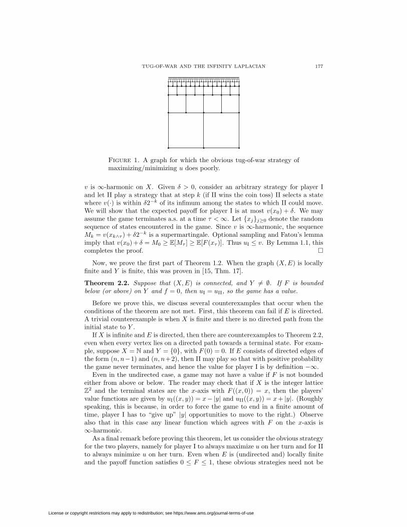
Figure 1. A graph for which the obvious tug-of-war strategy ofmaximizing/minimizing u does poorly.

v is ∞-harmonic on X. Given δ > 0, consider an arbitrary strategy for player Iand let II play a strategy that at step k (if II wins the coin toss) II selects a statewhere v(·) is within δ2−k of its infimum among the states to which II could move.We will show that the expected payoff for player I is at most v(x0) + δ. We mayassume the game terminates a.s. at a time τ < ∞. Let {xj}j≥0 denote the randomsequence of states encountered in the game. Since v is ∞-harmonic, the sequenceMk = v(xk∧τ ) + δ2−k is a supermartingale. Optional sampling and Fatou’s lemmaimply that v(x0)+ δ = M0 ≥ E[Mτ ] ≥ E[F (xτ )]. Thus uI ≤ v. By Lemma 1.1, thiscompletes the proof. �

Now, we prove the first part of Theorem 1.2. When the graph (X, E) is locallyfinite and Y is finite, this was proven in [15, Thm. 17].

Theorem 2.2. Suppose that (X, E) is connected, and Y = ∅. If F is boundedbelow (or above) on Y and f = 0, then uI = uII, so the game has a value.

Before we prove this, we discuss several counterexamples that occur when theconditions of the theorem are not met. First, this theorem can fail if E is directed.A trivial counterexample is when X is finite and there is no directed path from theinitial state to Y .

If X is infinite and E is directed, then there are counterexamples to Theorem 2.2,even when every vertex lies on a directed path towards a terminal state. For exam-ple, suppose X = N and Y = {0}, with F (0) = 0. If E consists of directed edges ofthe form (n, n−1) and (n, n+2), then II may play so that with positive probabilitythe game never terminates, and hence the value for player I is by definition −∞.

Even in the undirected case, a game may not have a value if F is not boundedeither from above or below. The reader may check that if X is the integer latticeZ2 and the terminal states are the x-axis with F ((x, 0)) = x, then the players’value functions are given by uI((x, y)) = x− |y| and uII((x, y)) = x + |y|. (Roughlyspeaking, this is because, in order to force the game to end in a finite amount oftime, player I has to “give up” |y| opportunities to move to the right.) Observealso that in this case any linear function which agrees with F on the x-axis is∞-harmonic.

As a final remark before proving this theorem, let us consider the obvious strategyfor the two players, namely for player I to always maximize u on her turn and for IIto always minimize u on her turn. Even when E is (undirected and) locally finiteand the payoff function satisfies 0 ≤ F ≤ 1, these obvious strategies need not be



optimal. Consider, e.g., the game shown in Figure 1, where X ⊂ R2 is given byX =

{v(k, j) : j = 1, 2, . . . ; k = 0, 1, . . . , 2j

}, v(k, j) = (2−jk, 1 − 2−j+1), and E

consists of edges of the form {v(k, j), v(k + 1, j)} and {v(k, j), v(2k, j + 1)}. Theterminal states are on the left and right edges of the square, and the payoff is 1 onthe left and 0 on the right. Clearly the function u(v(k, j)) = 1−k/2j (the Euclideandistance from the right edge of the square) is infinity harmonic, and by Corollary 2.3below, we have uI = u = uII. The obvious strategy for player I is to always moveleft, and for II it is to always move right. Suppose however that player I alwayspulls left and player II always pulls up. It is easy to check that the probabilitythat the game ever terminates when starting from v(k, j) is at most 2/(k + 2) (thisfunction is a supermartingale under the corresponding Markov chain). Thereforethe game continues forever with positive probability, resulting in a payoff of −∞ toplayer I. Thus, a near-optimal strategy for player I must be able to force the gameto end, and must be prepared to make moves which do not maximize u. (This is awell-known phenomenon, not particular to tug-of-war.)

Proof of Theorem 2.2. If F is bounded above but not below, then we may exchangethe roles of players I and II and negate F to reduce to the case where F is boundedfrom below. Since uI ≤ uII always holds, we just need to show that uII ≤ uI.Since player I could always pull towards a point in Y and thereby ensure thatthe game terminates, we have uI ≥ infY F > −∞. Let u = uI and write δ(x) =supy:y∼x |u(y) − u(x)|. Let x0, x1, . . . be the sequence of positions of the game.For ease of exposition, we begin by assuming that E is locally finite (so that thesuprema and infima in the definition of the ∞-Laplacian definition are achieved)and that δ(x0) > 0; later we will remove these assumptions.

To motivate the following argument, we make a few observations. In order toprove that uII ≤ uI, we need to show that player II can guarantee that the gameterminates while also making sure that the expected payoff is not much larger thanu(x0). These are two different goals, and it is not a priori clear how to combinethem. To resolve this difficulty, observe that δ(xj) is non-decreasing in j if players Iand II adopt the strategies of maximizing (respectively, minimizing) u at every step.As we will later see, this implies that the game terminates a.s. under these strategies.On the other hand, if player I deviates from this strategy and thereby reduces δ(xj),then perhaps player II can spend some turns playing suboptimally with respect tou in order to increase δ. Let X0 := {x ∈ X : δ(x) ≥ δ(x0)} ∪ Y . For n = 0, 1, 2, . . .let jn = max{j ≤ n : xj ∈ X0} and vn = xjn

, which is the last position in X0 up totime n. We will shortly describe a strategy for II based on the idea of backtrackingto X0 when not in X0. If vn = xn, we may define a backtracking move from xn

as any move to a neighbor yn of xn that is closer to vn than xn in the subgraphGn ⊂ (X, E) spanned by the vertices xjn

, xjn+1, . . . , xn. Here, “closer” refers tothe graph metric of Gn. When II plays the backtracking strategy, she backtrackswhenever not in X0 and plays to a neighbor minimizing uI when in X0.

Now consider the game evolving under any strategy for player I and the back-tracking strategy for II. Let dn be the distance from xn to vn in the subgraph Gn.Set

mn := u(vn) + δ(x0) dn .

It is clear that u(xn) ≤ mn, because there is a path of length dn from xn to vn in Gn

and the change in u across any edge in this path is less than δ(x0), by the definitionof X0. It is easy to verify that mn is a supermartingale, as follows. If xn ∈ X0, and



player I plays, then mn+1 ≤ u(xn) + δ(xn) = mn + δ(xn), while if II gets the turn,then mn+1 = u(xn) − δ(xn). If xn /∈ X0 and II plays, then mn+1 = mn − δ(x0). Ifxn /∈ X0 and player I does not play into X0, then mn+1 ≤ mn + δ(x0). The lastcase to consider is that xn /∈ X0 and player I plays into a vertex in X0. In such asituation,

mn+1 = u(xn+1) ≤ u(xn) + δ(xn) ≤ mn + δ(x0) .

Thus, indeed, mn is a supermartingale (bounded from below). Let τ denote thefirst time a terminal state is reached (so τ = ∞ if the game does not terminate).By the martingale convergence theorem, the limit limn→∞ mn∧τ exists. But whenplayer II plays we have mn+1 ≤ mn − δ(x0). Therefore, the game must terminatewith probability 1. The expected outcome of the game thus played is at mostm0 = u(x0). Consequently, uII ≤ u, which completes the proof in the case whereE is locally finite and δ(x0) > 0.

Next, what if E is not locally finite, so that suprema and infima might not beachieved? In this case, we fix a small η > 0, and use the same strategy as above,except that if xn ∈ X0 and II gets the turn, she moves to a neighbor at which uis at most η2−n−1 larger than its infimum value among neighbors of xn. In thiscase, mn + η 2−n is a supermartingale, and hence the expected payoff is at mostu(x0) + η. Since this can be done for any η > 0, we again have that uII ≤ u.

Finally, suppose that δ(x0) = 0. Let y ∈ Y , and let player II pull toward yuntil the first time a vertex x∗

0 with δ(x∗0) > 0 or x∗

0 ∈ Y is reached. After that, IIcontinues as above. Since u(x0) = u(x∗

0), this completes the proof. �

Corollary 2.3. If E is connected, Y = ∅ and sup |F | < ∞, then u = uI = uII isthe unique bounded ∞-harmonic function agreeing with F on Y .

Proof. This is an immediate consequence of Lemma 2.1, the remark that follows it,and Theorem 2.2. �

If E = {(n, n + 1) : n = 0, 1, 2, . . . }, Y = {0} and F (0) = 0, then u(n) = n is anexample of an (unbounded) ∞-harmonic function that is different from u.

2.2. Tug-of-war on graphs with running payoffs. Suppose now that f = 0.Then the analog of Theorem 2.2 does not hold without additional assumptions.For a simple counterexample, suppose that E is a triangle with self-loops at itsvertices (i.e., a player may opt to remain in the same position), that the vertex v0

is a terminal vertex with final payoff F (v0) = 0, and the running payoff is given byf(v1) = −1 and f(v2) = 1. Then the function given by u(v0) = 0, u(v1) = a − 1,u(v2) = a + 1 is a solution to ∆∞u = −2f , provided −1 ≤ a ≤ 1. The readermay check that uI is the smallest of these functions and uII is the largest. The gapof 2 between uI and uII appears because a player would have to give up a move(sacrificing one) in order to force the game to end. This is analogous to the Z2

example given in Section 2.1. Both players are earning payoffs in the interior of thegame, and moving to a terminal vertex costs a player a turn.

One way around this is to assume that f is either uniformly positive or uniformlynegative, as in the following analog of Theorem 2.2. We now prove the second halfof Theorem 1.2:

Theorem 2.4. Suppose that E is connected and Y = ∅. Assume that F is boundedfrom below and inf f > 0. Then uI = uII. If, additionally, f and F are bounded



from above, then any bounded solution u to ∆∞u = −2f with the given boundaryconditions is equal to u.

Proof. By considering a strategy for player I that always pulls toward a specificterminal state y, we see that infX uI ≥ infY F . By Lemma 1.1, ∆∞uI = −2f onX � Y . Let u be any solution to ∆∞u = −2f on X � Y that is bounded frombelow on X and has the given boundary values on Y .

Claim. uII ≤ u. In proving this, we may assume without loss of generality thatG �Y is connected, where G is the graph (X, E). Then if u = ∞ at some vertex inX �Y , we also have u = ∞ throughout X �Y , in which case the Claim is obvious.Thus, assume that u is finite on X �Y . Fix δ ∈ (0, inf f) and let II use the strategythat at step k, if the current state is xk−1 and II wins the coin toss, selects a statexk with u(xk) < infz:z∼xk−1 u(z) + 2−kδ. Then for any strategy chosen by player I,the sequence Mk = u(xk) + 2−kδ +

∑k−1j=0 f(xj) is a supermartingale bounded from

below, which must converge a.s. to a finite limit. Since inf f > 0, this also forcesthe game to terminate a.s. Let τ denote the termination time. Then

u(x0) + δ = M0 ≥ E(Mτ ) ≥ E

(u(xτ ) +

τ−1∑j=0

f(xj))

.

Thus this strategy for II shows that uII(x0) ≤ u(x0) + δ. Since δ > 0 is arbitrary,this verifies the claim. In particular, uII ≤ uI in X, so uII = uI.

Now suppose that sup F < ∞ and sup f < ∞, and u is a bounded solution to∆∞u = −2f with the given boundary values. By the claim above, u ≥ uII = uI.On the other hand, player I can play to maximize or nearly maximize u in everymove. Under such a strategy, she guarantees that by turn k the expected payoff isat least u(x0) − E[Q(k)] − ε, where Q(k) is 0 if the game has terminated by timek, and u(xk) otherwise. If the expected number of moves played is infinite, theexpected payoff is infinite. Otherwise, limk E[Q(k)] = 0, since u is bounded. Thus,uII = uI ≥ u in any case. �

3. Continuum value of tug-of-war on a length space

3.1. Preliminaries and outline. In this section, we will prove Theorem 1.3, The-orem 1.8 and Theorem 1.4. Throughout this section, we assume (X, d, Y, F, f) de-notes a tug-of-war game, i.e., X is a length space with distance function d, Y ⊂ Xis a non-empty set of terminal states, F : Y → R is the final payoff function, andf : X � Y → R is the running payoff function. We let xk denote the game state attime k in ε-tug-of-war.

It is natural to ask for a continuous-time version of tug-of-war on a length space.Precisely and rigorously defining such a game (which would presumably involvereplacing coin tosses with white noise, making sense of what a continuum no-look-ahead strategy means, etc.) is a technical challenge we will not undertake in thispaper (though we include some discussion of the small-ε limiting trajectory of ε-tug-of-war in the finite-dimensional Euclidean case in Section 7). But we can makesense of the continuum game’s value function u0 by showing that the value functionuε for the ε-step tug-of-war game converges as ε → 0.

The value functions uε do not satisfy any nice monotonicity properties as ε →0. In the next subsection we define two modified versions of tug-of-war whose



values closely approximate uε, and which do satisfy a monotonicity property alongsequences of the form ε2−n, allowing us to conclude that limn uε2−n

exists. Then weshow that any such limit is a bounded from below viscosity solution to ∆∞u = −2f ,and that any viscosity solution bounded from below is an upper bound on such alimit, so that any two such limits must be equal, which will allow us to prove thatthe continuum limit u0 = limε uε exists.

Because the players can move the game state almost as far as ε, either player canensure that d(xk, y) is “almost a supermartingale” up until the time that xk = y.When doing calculations it is more convenient to instead work with a related metricdε defined by

dε(x, y) := ε × (min # steps from x to y using steps of length < ε)

=

{0, x = y,

ε + ε�d(x, y)/ε�, x = y.

Since dε is the graph distance scaled by ε, it is in fact a metric, and either playermay choose to make dε(xk, y) a supermartingale up until the time xk = y.

3.2. II-favored tug-of-war and dyadic limits. We define a game called II-favored ε-tug-of-war that is designed to give a lower bound on player I’s expectedpayoff. It is related to ordinary ε-step tug-of-war, but II is given additional options,and player I’s running payoffs are slightly smaller. At the (i + 1)st step, player Ichooses a point z in Bε(xi) and a coin is tossed. If player I wins the coin toss, thegame position moves to a point, of player II’s choice, in (B2ε(z) ∩ Y ) ∪ {z}. (Ifd(z, Y ) ≥ 2ε, this means simply moving to z.) If II wins, then the game positionmoves to a point in B2ε(z) of II’s choice. The game ends at the first time τ forwhich xτ ∈ Y . Player I’s payoff is then −∞ if the game never terminates, andotherwise it is

(3.1) ε2τ∑

i=1

infy∈B2ε(zi)

f(y) + F (xτ ),

where zi is the point that player I targets on the ith turn, and f(y) is defined to bezero if y ∈ Y . We let vε be the value for player I for this game. Given a strategyfor player II in the ordinary ε-game, player II can easily mimic this strategy in theII-favored ε-game and do at least as well, so vε ≤ uε

I .Let wε be the value for player II of I-favored ε-tug-of-war, defined analogously

but with the roles of player I and player II reversed (i.e., at each move, II selectsthe target less than ε units away, instead of player I, etc., and the inf in the runningpayoff term in equation (3.1) is replaced with a sup, and games that never terminatehave payoff +∞). For any ε > 0 we have

vε ≤ uεI ≤ uε

II ≤ wε.

Lemma 3.1. For any ε > 0,

v2ε ≤ vε ≤ uεI ≤ uε

II ≤ wε ≤ w2ε.

Proof. We have already noted that vε ≤ uεI ≤ uε

II ≤ wε. We will prove thatv2ε ≤ vε; the inequality wε ≤ w2ε follows by symmetry. Consider a strategy S2ε

I

for a II-favored 2ε-tug-of-war. We define a strategy SεI for player I for the II-favored

ε-game that mimics S2εI as follows. Whenever strategy S2ε

I would choose a targetpoint z, player I “aims” for z for one “round,” which we define to be the time until



one of the players has won the coin toss two more times than the other player. By“aiming for z” we mean that player I picks a target point that, in the metric dε,is ε units closer to z than the current point. With probability 1/2, player I getstwo surplus moves before II, and then the game position reaches z (or a point inY ∩ B4ε(z)) before the game position exits B4ε(z). If player II gets two surplusmoves before player I, then the game position will be in B4ε(z). (See Figure 2.)The expected number of moves in this round of the II-favored ε-game is 4; and the

4ε

<ε<ε

2ε

z

xz

Figure 2. At the end of the round, player I reaches the targetz (or a point in Y ∩ B4ε(z)) with probability at least 1/2, andotherwise the state still remains within B4ε(z). During the firststep of the round, when player I has target z, the running payoffis the infimum of f over B2ε(z) ⊂ B4ε(z), and during any step ofthe round the infimum is over a subset of B4ε(z).

running payoff at each move is an ε2 times the infimum over a ball of radius 2ε thatis a subset of B4ε(z) (as opposed to (2ε)2 times the infimum over the whole ball).Hence strategy Sε

I guarantees for the II-favored ε-game an expected total payoffthat is at least as large as what S2ε

I guarantees for the II-favored 2ε-game. �

Thus vε converges along dyadic sequences: vε/2∞:= limn→∞ vε2−n

exists. Apriori the subsequential limit could depend upon the choice of the dyadic sequence,i.e., the initial ε.

The same argument can be used to show that vkε ≤ vε for positive integers k.

3.3. Comparing favored and ordinary tug-of-war. We continue with a pre-liminary bound on how far apart vε and wε can be. Let Lipε

Y F denote the Lipschitzconstant of F with respect to the restriction of the metric dε to Y . Since d ≤ dε,the Lipschitz constant LipY F of F with respect to d upper bounds Lipε

Y F .



Lemma 3.2. Let ε > 0. Suppose that LipεY F < ∞ and either

(1) f = 0 everywhere, or(2) |f | is bounded above and X has finite diameter.

Then for each x ∈ X and y ∈ Y ,

vε(x) ≥ F (y) − 2 ε LipεY F −

(Lipε

Y F + 2 (ε + diamX) sup |f |)dε(x, y).

Such an expected payoff is guaranteed for player I if she adopts a pull towards ystrategy, which at each move attempts to reduce dε(xt, y). Similarly a pull towardsy strategy for II gives

wε(x) ≤ F (y) + 2 ε LipεY F +

(Lipε

Y F + 2 (ε + diamX) sup |f |)dε(x, y).

Proof. Let player I use a pull towards y strategy. Let τ be the time at which Yis reached, which will be finite a.s. The distance dε(xk, y) is a supermartingale,except possibly at the last step, where player II may have moved the game stateto a terminal point up to a distance of 2ε from the target, even if player I wins thecoin toss. Thus E[dε(xτ , y)] < dε(x, y) + 2ε, whence

E[F (xτ )] ≥ F (y) −(dε(x, y) + 2ε

)Lipε

Y F.

If f = 0, then this implies vε(x) ≥ F (y) − (dε(x, y) + 2ε)LipεY F . If f = 0 and X

has finite diameter, then the expected number of steps before the game terminatesis at most the expected time that a simple random walk on the interval of integers[0, 1 + �diam(X)/ε�] (with a self-loop added at the right endpoint) takes to reach0 when started at j := dε(x, y)/ε, i.e., at most j

(3 + 2 �diam(X)/ε� − j

). Hence

E

[F (xτ ) +

τ−1∑i=0

ε2f(xi)]

≥ F (y) −(dε(x, y) + 2 ε

)Lipε

Y F + j(3 + 2 �diam(X)/ε� − j

)ε2 min(0, inf f)

≥ F (y) −(dε(x, y) + 2 ε

)Lipε

Y F − dε(x, y)(2 ε + 2 diam(X)

)sup |f |.

This gives the desired lower bound on vε(x). The symmetric argument gives theupper bound for wε(x). �

Next, we show that the lower bound vε on uεI is a good lower bound.

Lemma 3.3. Suppose F is Lipschitz, and either(1) f = 0 everywhere, or(2) f is uniformly continuous, X has finite diameter and inf |f | > 0.

Then ‖uεI − vε‖∞ → 0 as ε → 0. If f is also Lipschitz, then ‖uε

I − vε‖∞ = O(ε).

Note that since X is assumed to be a length space, the assumptions imply thatsign(f) is constant and sup |f | < ∞.

Proof. In order to prove that uεI is not much larger than vε, consider a strategy SI

for player I in ordinary ε-tug-of-war, which achieves an expected payoff of at leastuε

I −ε against any strategy for player II. We shortly describe a modified strategy SF

I

for player I playing the II-favored game, which does almost as well as SI does in theordinary game. To motivate SF

I , observe that a turn in the II-favored ε-tug-of-warcan alternatively be described as follows. Suppose that the position at the end ofthe previous turn is x. First, player I gets to make a move to an arbitrary pointz satisfying d(x, z) < ε. Then a coin is tossed. If player II wins the toss, she gets



to make two steps from z, each of distance less than ε. Otherwise, II gets to moveto an arbitrary point in B2ε(z) ∩ Y , but only if the latter set is non-empty. Thiscompletes the turn. The strategy SF

I is based on the idea that after a win in thecoin toss by II, player I may use her move to reverse one of the two steps executedby II (provided Y has not been reached).

As strategy SF

I is playing the II-favored game against player II, it keeps track ofa virtual ordinary game. At the outset, the II-favored game is in state xF

0 , as is thevirtual game. As long as the virtual and the favored game have not ended, eachturn in the favored game corresponds to a turn in the virtual game, and the virtualgame uses the same coin tosses as the favored game. In each such turn t, the targetzFt for player I in the favored game is the current state xt in the ordinary game. If

player I wins the coin toss, then the new game state xFt+1 in the favored game is his

current target zFt , which is the state of the virtual game xt, and the new state of

the virtual game xt+1 is chosen according to strategy SI applied to the history ofthe virtual game. If player II wins the toss and chooses the new state of the favoredgame to be xF

t+1, where necessarily d(xFt+1, xt) < 2 ε, then in the virtual game the

virtual player II chooses the new state xt+1 as some point satisfying d(xt+1, xt) < ε

and d(xt+1, xFt+1) < ε. Induction shows that d(xF

t , xt) < ε as long as both gamesare running, and thus the described moves are all legal.

If at some time the virtual game has terminated, but the favored game has not,we let player I continue playing the favored game by always pulling towards thefinal state of the virtual game. If the favored game has terminated, for the sake ofcomparison, we continue the virtual game, but this time let player II pull towardsthe final state of the favored game and let player I continue using strategy SI.

Let τF be the time at which the favored game has ended, and let τ be the timeat which the ordinary virtual game has ended. By Lemma 3.2, if τ < τF, thenthe conditioned expectation of the remaining running payoffs and final payoff toplayer I in the favored game after time τ , given what happened up to time τ , isat least F (xτ ) − O(ε) (here the implicit constant may depend on diamX, LipY Fand sup |f |). Likewise, uε

I ≤ wε from Lemma 3.1 and the second inequality fromLemma 3.2 show that if τF < τ , then the conditioned expectation of the remainingrunning and final payoffs in the virtual game is at most F (xF

τF) + O(ε).Set λ = λε := sup

{|f(x)− f(x′)| : x, x′ ∈ X � Y, d(x, x′) < 2 ε

}. Then λ = O(ε)

if f is Lipschitz and limε→0 λε = 0 if f is uniformly continuous. At each timet < τ ∧ τF, since zF

t = xt, the running payoff in the virtual game and in the favoredgame differ by at most ε2 λ. Lemmas 3.1 and 3.2 show that there is a constant C,which may depend on X, Y, f and F , but not on ε, such that −C ≤ vε ≤ uε

I ≤ C.Thus, in the case where sup f < 0, since SI guarantees a payoff of at least uε

I (x0)−ε,we have E[τF ∧ τ ] = O(ε−2). Assume that player II plays the II-favored game (upto time τ ∧ τF) using a strategy SF

II such that the expected payoff to player Iwho uses SF

I is at most vε + ε. Then, in the case where inf f > 0, we will haveE[τ∧τF] = O(ε−2), again. There is a strategy SII for player II in the ordinary game,which corresponds to the play of player II in the virtual game, when player I uses SI

and SF

I and player II uses SF

II in the favored game. (The description of the virtualgame defines SII for some game histories, and we may take an arbitrary extensionof this partial strategy to all possible game histories.) The above shows that theexpected payoff for player I in the ordinary game when player I uses SI and player IIuses SII differs from the expected payoff for player I in the favored game when



player I uses SF

I and player II uses SF

II by at most O(ε)+ λ ε2 E[τ ∧ τF] ≤ O(ε+ λ).Thus uε

I ≤ vε + O(ε + λ). Since uεI ≥ vε, the proof is now complete. �

Hence under the assumption of Lemma 3.3, limn→∞ uε2−n

I = vε/2∞.

3.4. Dyadic limits satisfy quadratic comparison. We start by showing thatuε

I almost satisfies (−2f)-quadratic comparison from above.

Lemma 3.4. Let ε > 0, let V be an open subset of X � Y and write Vε = {x :Bε(x) ⊂ V }. Suppose that ϕ(x) = Q(d(x, z)) is a quadratic distance function thatis -increasing on V , where Q(r) = ar2 + br + c satisfies

(3.2) a ≤ − supx∈Vε

f(x).

Also suppose that supVεf ≥ 0 or diam(V ) < ∞. If the value function uε

I for player Iin ε-tug-of-war satisfies uε

I ≤ ϕ on V \Vε, then uεI ≤ ϕ on Vε.

Proof. Fix some δ > 0. Consider the strategy for player II that from a statexk−1 ∈ Vε at distance r = d(xk−1, z) from z pulls to state z (if r < ε) or elsemoves to reduce the distance to z by “almost” ε units, enough to ensure thatQ(d(xk, z)) < Q(r − ε) + δ2−k. If r < ε, then z ∈ V , whence Q(t) = at2 + c witha ≥ 0. In this case, if II wins the toss, then xk = z, whence ϕ(xk) = Q(0) ≤ Q(r−ε).Thus for all r ≥ 0, regardless of what strategy player I adopts,

E[ϕ(xk) | xk−1] − δ2−k−1 ≤ Q(r + ε) + Q(r − ε)2

= Q(r) + a ε2 = ϕ(xk−1) + a ε2 .

Setting τ := inf{k : xk /∈ Vε}, we conclude that Mk := ϕ(xk∧τ )−a ε2(k∧ τ )+δ 2−k

is a supermartingale.Suppose that player I uses a strategy with expected payoff larger than −∞. (If

there is no such strategy, the assertion of the lemma is obvious.) Then τ < ∞ a.s.We claim that

(3.3) E[Mτ ] ≤ M0 .

Clearly this holds if τ is replaced by τ ∧ k. To pass to the limit as k → ∞, considertwo cases:

• If a ≤ 0, then since ϕ is -increasing on V , it is also bounded from below onV . Consequently, Mk is a supermartingale bounded from below, so (3.3)holds.

• If a > 0, then supVεf < 0, by (3.2). By assumption therefore diamV <

∞, which implies supV |ϕ| < ∞. If E[τ ] = ∞, we get E[Mτ ] = −∞,and hence (3.3) holds. On the other hand, if E[τ ] < ∞, then dominatedconvergence gives (3.3).

Since uεI (xτ ) ≤ ϕ(xτ ), we deduce that

uεI (x0) ≤ sup

SI

E

[ϕ(xτ ) +

τ−1∑t=0

f(xt)] (3.2)

≤ supSI

E[Mτ ] ≤ M0 = ϕ(x0) + δ ,

where SI runs over all possible strategies for player I with expected payoff largerthan −∞. Since δ > 0 was arbitrary, the proof is now complete. �



In order for uεI to satisfy (−2f)-quadratic comparison (from above), we would

like to know that if uεI ≤ ϕ on the boundary of an open set, then this (almost)

holds in a neighborhood of the boundary, so that we can apply the above lemma.To do this we prove a uniform Lipschitz lemma:

Lemma 3.5 (Uniform Lipschitz). Suppose that F is Lipschitz, and either(1) f = 0 everywhere, or(2) |f | is bounded from above and X has finite diameter.

Then for each ε ∈ (0, diamX), uεI and uε

II are Lipschitz on X w.r.t. the metric dε

with the Lipschitz constant depending only on diamX, sup |f | and LipY F .

Proof. By symmetry, it suffices to prove this for uεI . Set

L := 3 LipεY F + 4 diamX sup |f |.

Let x, y ∈ X be distinct. If x, y ∈ Y , then∣∣uε

I (x) − uεI (y)

∣∣ =∣∣F (x) − F (y)

∣∣ ≤Lipε

Y F dε(x, y). If x ∈ X � Y and y ∈ Y , Lemmas 3.2 and 3.1 give

(3.4)∣∣uε

I (x) − uεI (y)

∣∣ =∣∣uε

I (x) − F (y)∣∣ ≤ L dε(x, y) , x ∈ X � Y, y ∈ Y .

Now suppose x, y ∈ X � Y . Set Y ∗ = Y ∪ {y}, F ∗ = F on Y and F ∗(y) = uεI (y).

Then, clearly, the value of uεI (x) for the game where Y is replaced by Y ∗ and

F is replaced by F ∗ is the same as for the original game. By (3.4), we haveLipε

Y ∗(F ∗) ≤ L. Consequently, (3.4) gives∣∣uεI (x) − uε

I (y)∣∣ =

∣∣uεI (x) − F ∗(y)

∣∣ ≤ (3 L + 2 (ε + diamX) sup |f |

)dε(x, y)

≤ 4 L dε(x, y) ,

which completes the proof. �

Lemma 3.6. Suppose F is Lipschitz and inf F > −∞, and either (1) f = 0identically or else (2) inf f > 0, f is uniformly continuous, and X has finite diam-eter. Then the subsequential limit vε/2∞

= limn→∞ vε2−n

satisfies (−2f)-quadraticcomparison on X � Y .

Proof. By Theorems 2.2 and 2.4, uεI = uε

II, so from Lemma 3.3 we have ‖wε −vε‖∞ → 0 as ε → 0. Thus limn→∞ wε2−n

= vε/2∞.

Note that the hypotheses imply that |f | is bounded. Consider an open V ⊂X �Y and an -increasing quadratic distance function ϕ on V with quadratic terma ≤ − supy∈V f(y), such that ϕ ≥ vε/2∞

on ∂V . We must show that ϕ ≥ vε/2∞on

V . Since ‖wε−vε‖∞ → 0, we have by Lemma 3.1 that vε2−n

converges uniformly tovε/2∞

. So for any δ > 0, if n ∈ N is large enough, then vε2−n ≤ ϕ + δ on ∂V . Notealso that ϕ is necessarily uniformly continuous on V . (If diamV < ∞ or a = 0, thisis clear. Otherwise, f = 0 and a < 0. However, a < 0 implies that diamV < ∞,since ϕ is -increasing on V .) Hence, by the uniform Lipschitz lemma, Lemma 3.5,uε2−n

I ≤ ϕ + 2 δ on V � Vε2−n for all sufficiently large n ∈ N, where we use thenotation of Lemma 3.4. By that lemma uε2−n

I ≤ ϕ+2 δ on all of V . Letting n → ∞and δ → 0 shows that vε/2∞

satisfies (−2f)-quadratic comparison from above.To prove quadratic comparison from below, note that the only assumptions which

are not symmetric under exchanging the roles of the players are inf F > −∞ andinf f > 0. However, we only used these assumptions to prove wε/2∞

= vε/2∞.

Consequently, comparison from below follows by symmetry. �



3.5. Convergence.

Lemma 3.7. Suppose that v is continuous and satisfies (−2f)-quadratic compar-ison from below on X � Y , and that f is locally bounded from below. Let δ > 0.Then in II-favored ε-tug-of-war, when player I (using any strategy) targets point zi

on step i, player II may play to make Mt∧τεa supermartingale, where

Mt := v(xt) + ε2t∑

i=1

infy∈B2ε(zi)

f(y) + δ2−t

and τε := inf{t : d(xt, Y ) < 3 ε}.

Proof. Let z = zt be the point that player I has targeted at time t. Assume thatt < τε. We define the following:

(1) α := inf{f(x) : x ∈ B2ε(z)},(2) A := inf{v(x) : x ∈ B2ε(z)} (the infimum value of v that II can guarantee

if II wins the coin toss),(3) β := v(z)+A

2 + α ε2, and

(4) Q(r) := −αr2 + A−v(z)+4αε2

2ε r + v(z) (Q(0) = v(z), Q(2ε) = A, Q(ε) = β,and Q′′ = −2α).

Player II can play so that E[v(xt)

∣∣ zt and all prior events]≤ (v(z) + A)/2 + δ2−t,

i.e., so that E[Mt

∣∣ zt and prior events]− Mt−1 ≤ β − v(xt−1). We will show

that whenever d(x, z) < ε we have v(x) ≥ β, and then it will follow that M is asupermartingale. There are two cases to check, depending on whether α > 0 orα ≤ 0:

Suppose α ≤ 0. Note that A ≤ v(z). If v(z) = A, the inequality v(x) ≥ β onBε(z) follows from α ≤ 0 and the definition of β. Assume therefore that v(z) > A.Then Q′(ε) = (A − v(z))/(2ε) < 0. Thus Q is decreasing on [0, ε]. Let r0 ∈ [ε, 2 ε]be the point where Q attains its minimum in [ε, 2 ε]. Then Q is decreasing on [0, r0].Set V := Br0(z) � {z}. We have v(z) = Q(0) = Q

(d(z, z)

), and for x ∈ ∂Br0(z)

we have v(x) ≥ A = Q(2 ε) ≥ Q(r0) = Q(d(x, z)

). Thus, v(x) ≥ Q

(d(x, z)

)for x ∈ ∂V . Since v satisfies (−2f)-quadratic comparison from below, and Q′′ =−2 α ≥ supx∈V −2 f(x), we get v(x) ≥ Q

(d(x, z)

)for x ∈ V . In particular, for

x ∈ Bε(z) one has v(x) ≥ Q(d(x, z)

)≥ Q(ε) = β.

Now suppose α > 0. The function L0(x) = −α d(x, z)2 + α(2 ε)2 + A is a lowerbound for v on ∂B2ε(z), and hence applying (−2f)-quadratic comparison in B2ε(z)with L0(·) gives v(z) ≥ L0(z) = A + 4 α ε2. Therefore, Q′(0) = (A − v(z) +4αε2)/(2ε) ≤ 0, which together with Q′′ < 0 implies that Q is decreasing on [0, 2ε].By applying (−2f)-quadratic comparison on B2ε(z)�{z} we see that for x ∈ Bε(z)we have v(x) ≥ Q(d(x, z)) ≥ Q(ε) = β. �Lemma 3.8. Suppose that F is Lipschitz, and either

(1) f = 0 everywhere, or(2) |f | is bounded from above and X has finite diameter.

Also suppose that v : X → R is continuous, satisfies (−2f)-quadratic comparisonfrom below on X � Y , v ≥ F on Y , and inf v > −∞. Then vε ≤ v for all ε.

Proof. The idea is for player II to make the M defined in Lemma 3.7 a super-martingale, but we need to pick a stopping time τ such that E[Mτ ] ≤ M0, whilevε(xτ ) is unlikely to be much larger than v(xτ ). Let W := {x ∈ X : d(x, Y ) ≥ 3 ε}



and let τε be defined as in Lemma 3.7; that is, τε := inf{t ∈ N : xt /∈ W}. Setλε := supX�W (vε − v), and let δ > 0. We first show

(3.5) vε ≤ v + λε + δ .

In the case that f = 0, the supermartingale M is bounded from below, so we canchoose τ = τε. Player I is compelled to ensure τ < ∞. Conditional on the gameup to time τ , player I cannot guarantee a conditional expected payoff better thanvε(xτ ) + δ 2−τ ≤ Mτ + λε. Since E[Mτ ] ≤ M0 = v(x0) + δ, we get (3.5), as desired.

In the case f = 0, we let τn := τε ∧ n, where n ∈ N. Then E[Mτn] ≤ M0. Note

that sup vε < ∞ follows from diamX < ∞, vε ≤ uεI and Lemma 3.5. Suppose

player II makes M a supermartingale up until time τn. Given play until time τn,player II may make sure that the conditional expected payoff to player I is at most

δ 2−τn + vε(xτn) + ε2

τn∑i=1

infy∈B2ε(zi)

f(y) .

Taking expectation and separating into cases in which xτn∈ W or not, we get

vε(x0) ≤ E

[v(xτn

) + ε2τn∑i=1

infy∈B2ε(zi)

f(y)]

+ λε + δ 2−τn

+ Pr[xτn∈ W ] sup

W

(vε(x) − v(x)

).

Since E[Mτn] ≤ M0 = v(x0) + δ, this gives

vε(x0) ≤ v(x0) + δ + λε + Pr[xτn∈ W ] sup

W

(vε(x) − v(x)

).

The first term above is < E[Mτn] ≤ M0 = v(x0) + δ, independent of n. Player I

is compelled to play a strategy that ensures τ∞ is finite a.s., since otherwise thepayoff is −∞ < v(x). With such a strategy, Pr[xτn

∈ W ] → 0 as n → ∞, and sincev is bounded from below and sup vε < ∞, the last summand tends to 0 as n → ∞.Thus, we get (3.5) in this case as well.

Next, we show that lim supε↘0 λε ≤ 0. Let y ∈ Y , and set Q(r) = a r2 + b r + c,where a := sup |f |, b < b∗ := −2 sup |f | diamX − LipF , and c := F (y). Letϕ(x) := Q

(d(x, y)

). Then ϕ(y′) ≤ F (y′) ≤ v(y′) for y′ ∈ Y . Since v satisfies

comparison from below and ϕ is -decreasing , we get v(x) ≥ ϕ(x) on X. Thus,if x ∈ B3ε(y), then v(x) ≥ F (y) + b∗ d(x, y) ≥ F (y) + 3 b∗ ε. In conjunction withLemma 3.5, this implies that lim supε↘0 λε ≤ 0. Choosing δ = ε and taking ε to 0therefore gives in (3.5) lim supε↘0 vε ≤ v. However, the inequality v2ε ≤ vε fromLemma 3.1 implies vε ≤ lim supε′↘0 vε′ ≤ v, completing the proof. �

Proof of Theorem 1.3. First, suppose that F is Lipschitz. Let ε, ε′ > 0. Let v :=limn→∞ vε2−n

and v′ := limn→∞ vε′2−n

. We know that these limits exist fromLemma 3.1. Lemma 3.3 tells us that ‖uε

I − vε‖∞ → 0 as ε → 0. Since theassumptions of that lemma are player-symmetric, we likewise get ‖uε

II−wε‖∞ → 0.From Theorems 2.2 and 2.4 (possibly with the roles of the players interchanged) weknow that uε

I = uεII, and hence the above gives ‖vε − wε‖∞ → 0. By Lemma 3.1,

vε ≤ v ≤ wε and vε ≤ uεI ≤ wε, and so we conclude that ‖vε − v‖∞ → 0 and

‖uεI − v‖∞ → 0. Note that the assumptions imply that sup |f | < ∞. Therefore,

from Lemma 3.5 and ‖uεI − v‖∞ → 0 we conclude that v is Lipschitz. Precisely

the same argument gives ‖vε − v‖∞ = O(ε) if f is also assumed to be Lipschitz,



and similar estimates also hold for ‖vε′ − v′‖∞. Note that the assumptions implythat F is bounded if f = 0. Lemma 3.6 (applied possibly with the roles of theplayers reversed) tells us that v′ satisfies (−2f)-quadratic comparison on X � Y .Clearly inf v′ > −∞. (If f = 0 identically, then inf v′ ≥ inf F , while if diamX < ∞,we may use the fact that v′ is Lipschitz.) Thus, Lemma 3.8 implies that vε ≤ v′.Consequently, v ≤ v′. By symmetry v′ ≤ v, and hence v = v′. This completes theproof in the case where F is Lipschitz.

Using the result of Lemma 3.9 below, we know that for every δ > 0 there is aLipschitz Fδ : Y → R such that ‖F − Fδ‖∞ < δ. Then the Lipschitz case appliesto the functions Fδ ± δ in place of F . Since the game value uε for F is boundedbetween the corresponding value with Fδ + δ and Fδ − δ, and the latter two valuesdiffer by 2δ, the result easily follows. �

Lemma 3.9. Let X be a length space, and let F : Y → R be defined on a non-emptysubset Y ⊂ X. The following conditions are equivalent:

(1) F is uniformly continuous and sup{(F (y)−F (y′))/ max{1, d(y, y′)} : y, y′ ∈Y } < ∞.

(2) F extends to a uniformly continuous function on X.(3) There is a sequence of Lipschitz functions on Y tending to F in ‖ · ‖∞.

Proof. We start by assuming (1) and proving (2). Let ϕ(δ) := sup{F (y) − F (y′) :

d(y, y′) ≤ δ, y, y′ ∈ Y}

and ϕ(t) := sup{t ϕ(δ)/δ : δ ≥ t

}. We now show that

limt↘0 ϕ(t) = 0. Let ε > 0, and let δε > 0 satisfy ϕ(δε) < ε. Such a δε existsbecause F is uniformly continuous. Condition (1) implies that M := sup{ϕ(δ)/δ :δ ≥ δε} < ∞. For t < (ε/M) ∧ δε, we have

ϕ(t) = sup{t ϕ(δ)/δ : δε ≥ δ ≥ t

}∨ sup

{t ϕ(δ)/δ : δ > δε

}≤ ϕ(δε) ∨ (t M) ≤ ε ,

which proves that limt↘0 ϕ(t) = 0. Two other immediate properties of ϕ whichwe will use are that F (y) − F (y′) ≤ ϕ

(d(y, y′)

)≤ ϕ

(d(y, y′)

)holds for y, y′ ∈ Y

and ϕ(s t) ≥ s ϕ(t) when s ∈ [0, 1] and t ≥ 0. It follows that ϕ is subadditive:ϕ(a) + ϕ(b) ≥ a ϕ(a + b)/(a + b) + b ϕ(a + b)/(a + b) = ϕ(a + b) for a, b ≥ 0.

Now for x ∈ X set u(x) := inf{F (y) + ϕ(d(y, x)) : y ∈ Y

}. Then u = F on Y .

We now prove

(3.6) u(x) − u(x′) ≤ ϕ(d(x, x′)

)for x, x′ ∈ X. Indeed, let y′ ∈ Y . Then

u(x) − F (y′) − ϕ(d(y′, x′)

)≤ F (y′) + ϕ

(d(y′, x)

)− F (y′) − ϕ

(d(y′, x′)

)= ϕ

(d(y′, x)

)− ϕ

(d(y′, x′)

).

Consequently, subadditivity and monotonicity of ϕ gives

u(x) − F (y′) − ϕ(d(y′, x′)

)≤ ϕ

(∣∣d(x, y′) − d(x′, y′)∣∣) ≤ ϕ

(d(x, x′)

).

Taking the supremum over all y′ ∈ Y then implies (3.6). Therefore, u is uniformlycontinuous and (2) holds.

We now assume (2) and prove (3). Let u : X → R be a uniformly continuousextension of F to X. It clearly suffices to approximate u by Lipschitz functionson X in ‖ · ‖∞. For x ∈ X let uL(x) := inf

{u(x′) + L d(x, x′) : x′ ∈ X

}. The

same argument which was used above to prove (3.6) now shows that Lip(uL) ≤ L.



Clearly, uL(x) ≤ u(x). Let ϕ(t) := sup{u(x)− u(x′) : d(x, x′) ≤ t

}for t ≥ 0. Since

X is a length space, ϕ is subadditive. Let t > 0 and k := �d(x, x′)/t�. Then

u(x) − u(x′) − L d(x, x′) ≤ ϕ(d(x, x′)

)− L d(x, x′) ≤ ϕ

((k + 1) t

)− L k t .

Taking the supremum over all x′ and using the subadditivity of ϕ therefore gives

u(x) − uL(x) ≤ supk∈N

(ϕ((k + 1) t

)− L k t

)≤ ϕ(t) + sup

k∈N

k(ϕ(t) − L t

).

Therefore, u(x) − uL(x) ≤ ϕ(t) once L > ϕ(t)/t. Since inft>0 ϕ(t) = 0 and uL ≤u(x), this proves (3).

The passage from (3) to (1) is standard, and therefore omitted. This concludesthe proof. �

Proof of Theorem 1.8. Lemma 3.9 tells us that F extends to a uniformly continu-ous function on X and that it can be approximated in ‖·‖∞ by Lipschitz functions.We know from Theorem 1.3 that the continuum value u exists and is uniformlycontinuous. Suppose first that F is Lipschitz. Lemma 3.6 (applied possibly withthe roles of the players reversed) says that u satisfies (−2f)-quadratic comparisonon X �Y . If F is not Lipschitz, we may deduce the same result by approximating Ffrom below by Lipschitz functions and observing that a monotone non-decreasing‖ · ‖∞-limit of functions satisfying (−2f)-quadratic comparison from above alsosatisfies (−2f)-quadratic comparison from above, and making the symmetric argu-ment for comparison from below. Now suppose that u is as in the second part of thetheorem. This clearly implies inf u > −∞. Now Lemma 3.8 gives u ≤ u (again, wemay need to first approximate F by Lipschitz functions). The uniqueness followsdirectly. �

Proof of Theorem 1.4. If x ∈ X�Y and y ∈ Y , then from Lemma 3.2 it follows that∣∣u(x) − u(y)∣∣ ≤ LipY F d(x, y). Let U ⊂ X � Y be open and define F ∗(x) = u(x)

for x ∈ Y ∪ ∂U . It is clear that the continuum value u∗ of (X, d, Y ∪ ∂U, F ∗, 0) isthe same as u, since any player may first play a strategy that is appropriate for the(X, d, Y ∪ ∂U, F ∗, 0) game, and once Y ∪ ∂U is hit, start playing a strategy that isappropriate for the original game. The above argument shows that

∣∣u(x)−u(y)∣∣ ≤

d(x, y) Lip∂Uu if y ∈ ∂U and x ∈ U . In particular, Lip∂U∪{x}u = Lip∂Uu, whichimplies LipUu = Lip∂Uu; that is, u is AM in X � Y .

Now suppose that u∗ : X → R is an AM extension of F and sup |F | < ∞.Lemma 1.6 tells us that u∗ satisfies comparison with distance functions. Observethat the proof of Lemma 3.8 shows that in the case f = 0 we may replace thehypothesis that v satisfies 0-quadratic comparison from below on X � Y by thehypothesis that v satisfies comparison with distance functions from below (sinceonly comparisons with distance functions are used in this case). Thus, u ≤ u∗.Similarly, u ≥ u∗, which implies the required uniqueness statement and completesthe proof. �

4. Harmonic measure for ∆∞

Here, we present a few estimates of the ∞-harmonic measure ω∞. Before provingTheorem 1.5, we consider the ∞-harmonic of porous sets. Recall that a set S ina metric space Z is α-porous if for every r ∈ (0, diamZ) every ball of radius rcontains a ball of radius α r that is disjoint from S. An example of a porous set



is the ternary Cantor set in [0, 1]. We start with a general lemma in the setting oflength spaces.

Lemma 4.1. Suppose X is a length space and 0 ≤ F ≤ 1 on the terminal states Y ,where F : Y → R is continuous. Let S := suppF . Suppose that for some integer kand positive constants ε0, dmin and γ ∈ (0, 1), for every x ∈ X with d(x, S) ≥ dmin,there is a sequence of points x = z0, . . . , zk such that zk ∈ Y , F (zk) = 0, and

d(zi, S) ≥ 2 d(zi, zi−1) + 2 ε0 + γ d(z0, S)

for i = 1, . . . , k. Then the AM extension u of F satisfies

0 ≤ u(x) ≤ (1 − 2−k)logγ(dmin/d(x,S)).

Proof. We will obtain bounds on uε(x) that are independent of ε (as long as ε ∈(0, ε0)), and these yield bounds on u(x). Since uε ≥ 0, we need only give a goodstrategy for player II to obtain an upper bound on uε(x). The idea is for player IIto always have a “plan” for reaching a terminal state at which F is 0, while stayingaway from the terminal states at which F is non-zero. A plan consists of a sequenceof points z0, z1, . . . , zk, where z0 is the game state when the plan was formed,zk ∈ Y , and F (zk) = 0. As soon as the game state reaches zi, player II startspulling towards zi+1. If player I is lucky and gets many moves, player II may haveto give up on the plan and form a new plan. When tugging towards zi, we supposethat player II gives up and forms a new plan as soon as dε(xt, zi) = 2dε(zi, zi−1),and otherwise plays to ensure that dε(xt, zi) is a supermartingale. While tuggingtowards zi, the plan will be aborted at that stage with probability at most 1/2, sowith probability at least 2−k the plan is never aborted and succeeds in reaching zk.

Suppose player II aborts the plan at time t while tugging towards zi, and formsa new plan starting at z′0 = xt. Then d(xt, zi) ≤ dε(xt, zi) = 2 dε(zi, zi−1) ≤2 d(zi, zi−1) + 2 ε, so

d(xt, S) ≥ d(zi, S) − d(xt, zi) ≥ d(zi, S) − [2d(zi, zi−1) + 2ε] ≥ γ d(z0, S),

so the game state remains far from S. Since player II can always find a short plan(length at most k) when the distance from S is at least dmin, player I gets to S

with probability at most (1−2−k)�logγ(dmin/d(x0,S))�, which yields the desired upperbound. �

The reader may wish to check that the lemma implies limδ↘0 ω∞(Aδ) = 0 in thesetting of Theorem 1.5 (i.e., when X is the unit ball in Rn, n > 1, Y = ∂X and Aδ

is a spherical cap of radius δ).We are now ready to state and prove an upper bound on the ∞-harmonic measure

of neighborhoods of porous sets.

Theorem 4.2. Let X ⊂ Rn, n > 1, be the closed unit ball and let Y be its boundary,the unit sphere. Let α ∈ (0, 1/2) and let δ > 0. Let S be an α-porous subset of Y ,and let Sδ be the closure of the δ-neighborhood of S. Then

ω(0,Y,X)∞ (Sδ) ≤ δαO(1)

.

Of course, in the above, S is α-porous as a subset of Y . (Every subset of Y is(1/3)-porous as a subset of X.)

Proof. The plan is to use the lemma, of course. Let dmin := 2 δ/α. Let z0 ∈ X �Y ,and suppose that d0 := d(z0, S) ≥ dmin. Let y0 ∈ Y be a closest point to z0 on Y .



Inside Bd0(y0) ∩ Y there is a point y1 such that Bαd0(y1) ∩ S = ∅. (See Figure 3.)Therefore, d(y1, Sδ) ≥ α d0 − δ ≥ α d0/2. We define the sequence zj inductively, asfollows. If d(zj , Sδ) ≥ 3 d(zj , Y ), then we take zj+1 to be any closest point to zj

on Y . Otherwise, let zj+1 be the point on the line segment from zj to y1 whosedistance from zj is d(zj , y1)/10. It can be checked that after k = O(− log α) stepsthe sequence hits Y � S and that the assumptions of the lemma hold with this k,with γ = α/10 and with some ε0 > 0, independent of z0. The theorem now easilyfollows from the lemma. �

We now proceed to study the ∞-harmonic measure of spherical caps.

Proof of Theorem 1.5. It turns out to be more convenient to work with −Aδ ={−y : y ∈ Aδ} in place of Aδ. By an obvious comparison argument, it is sufficient

z0

y0y1

Figure 3. The terminal states are the unit sphere, and the sup-port of F is Sδ, the δ-neighborhood of a porous set on the unitsphere. From a starting point z0, player II finds a point y1 on thesphere that is near the closest point y0 on the sphere but far fromSδ. Player II then tugs towards y1 along a sequence of points, andthen when it gets much closer to the sphere than to Sδ, it tugsstraight to the sphere.



to estimate u(0), where u = uδ is the AM function in X � Y with boundary values

F (y) :=

⎧⎪⎨⎪⎩1 , y ∈ −Aδ ,

0 , d(y,−Aδ) > δ ,

1 − d(y,−Aδ) δ−1 , 0 < d(y,−Aδ) ≤ δ .

The function u is invariant under rotations of X preserving (1, 0, . . . , 0) ∈ Rn.Therefore, u is also AM in R2 ∩ X. Thus, we henceforth restrict ourselves to thecase n = 2, with no loss of generality.

Aronsson [3] constructed a family of viscosity solutions Gm to ∆∞u = 0 inR

2� {0} that are separable in polar coordinates: Gm(r, θ) = rm2/(2m−1)hm(θ) (for

m ∈ Z). We are interested in the m = −1 solution, which may be written as

(4.1) G =[

cos θ (1 − | tan(θ/2)|4/3)2

1 + | tan(θ/2)|4/3 + | tan(θ/2)|8/3

]1/3

r−1/3.

Observe that when −π/2 ≤ θ ≤ π/2 this solution is non-negative, and G ≥ c r−1/3

when θ ∈ [−π/4, π/4], say, where c > 0 is some fixed constant. Then F ≤ O(1) Gδ,where

Gδ(x, y) = δ1/3 G(x + 1 + 2 δ, y) .

Since u(0) is monotone in F , and Gδ satisfies ∆∞Gδ = 0, it follows that u(0) ≤O(1) Gδ(0) = O(δ1/3).

We now show that the bound u(0) = O(δ1/3) is tight. It is easy to see, usingcomparison with a cone centered at (−1, 0), say, that u(−1+δ/10, 0) > c > 0, wherec is a constant that does not depend on δ. Comparison with a cone centered at anypoint z in the unit disk shows that u(z′) ≥ u(z)/2 if |z − z′| ≤ (1 − |z|)/2. Usingsuch estimates, it is easy to see that there is a constant c′ > 0 such that u ≥ c′ onthe disk B of radius δ centered at q := (−1 + 2δ, 0), provided that δ < 1/4, say.Now consider the function

G∗δ(x, y) = c′ δ1/3 G

((x, y) − q

).

By the choice of the constant c′, we have G∗δ ≤ u on ∂B, since G ≤ r−1/3 in R

2�{0}.

If (r′, θ′) denote the polar coordinates centered at q, the center of B, and (r, θ)denote the standard polar coordinates centered at 0, then 2 |θ′| ≥ π − |θ − π| whenr = 1, and we choose θ′ ∈ [−π, π). Also, r′ is bounded from below by a constanttimes |θ− π| when θ ∈ [0, 2π] and r = 1. Since |G| ≤ O(1)

((π/2)− |θ|

)r−1/3 when

θ ∈ [−π, π), it follows that on the unit circle

G∗δ ≤ O(1)

((π/2) − |θ′|

)(r′)−1/3 ≤ O(1) δ1/3 |θ − π|2/3 ≤ O(δ1/3) .

Therefore G∗δ − O(δ1/3) ≤ u on the boundary of the unit circle, as well as on ∂B.

Consequently, u ≥ G∗δ − O(δ1/3) in the complement of B in the unit disk. This

implies that there is some r ∈ (0, 1) such that uδ(−r, 0) ≥ δ−1/3 for all sufficientlysmall δ. The required estimate uδ(0) ≥ Θ(δ−1/3) now follows by several applicationsof comparison with cones (the number of which depends on r), similar to the aboveargument estimating a lower bound for u on B. �

One could also try to use Aronsson’s other solutions Gm to bound ∞-harmonicmeasure of certain sets in other domains. Also, Aronsson has some explicit solutionsfor ∆pu = 0, which may serve a similar purpose.



5. Counterexamples

5.1. Tug-of-war games with positive payoffs and no value. Here we give thepromised counterexample showing that the hypothesis inf f > 0 in Theorem 1.2cannot be relaxed to f > 0. As we later point out, a similar construction works inthe continuum setting of length spaces.

The comb game is tug-of-war with running payoffs on an infinite graph shapedlike a comb, as shown in Figure 4. The comb is defined by an infinite sequence ofpositive integers �0, �1, �2 . . ., and has states (vertices) {(x, y) ∈ Z

2 : 0 ≤ x and 0 ≤y ≤ �x}. The edges of the comb are of the form (x, y) ∼ (x, y + 1) and (x, 0) ∼(x + 1, 0), giving the graph the shape of a comb, where the xth tooth of the combhas length �x. The running payoff f(x, y) is 1/�x if y = 0 and zero otherwise. (Laterwe will consider a variation where f > 0 everywhere.) The terminal states are thestates of the form (x, �x), and the terminal payoff F is zero on all terminal states.

Figure 4. A comb.

Lemma 5.1. For any comb (choice of the sequence {�x}), we have uI(0, 0) = 2.

Proof. First we argue that uI(0, 0) ≥ 2. Denote by ψ(t) :=∑t−1

i=0 f(xi, yi) theaccumulated running payoff. Fix a large B > 0 and equip player I with the followingstrategy: at all times t < τ for which ψ(t) < B, player I pulls down if yt = 0, leftif yt = 0 and xt = 0, and right if (xt, yt) = (0, 0); if ψ(xt) ≥ B, then player I pullstoward the closest terminal state. Define the termination time τ = inf{t : yt = �xt

}and also the stopping time σ0 = inf{t : xt = 0}∧τ . Fix any strategy for player II andobserve that {xt∧σ0}t≥0 is a non-negative supermartingale, which must convergea.s.; therefore, from any initial state, σ0 < ∞ a.s.; therefore, the stopping timeσ = inf{t : ψ(t) ≥ B} ∧ τ is almost surely finite, whence τ < ∞ a.s. as well.

Consider the process

Mt = 2(1 − yt/�xt) + ψ(t) .

Then Mt∧σ is a submartingale. Note that if yσ = 0, then Mσ = ψ(σ) + 2 andψ(σ) ≥ B, while if yσ > 0, then σ = τ and Mσ = ψ(σ). In any case, Mσ ≤ψ(σ)(1 + 2/B). Thus by optional stopping,

2 = M0 ≤ EMσ ≤ (1 +2B

)Eψ(σ) ≤ (1 +2B

)uI(0, 0).



Next, to show that uI(0, 0) ≤ 2, suppose that player II adopts the strategyof always pulling up, and player I knows this and seeks to maximize her payoff.Because player II always pulls up, Mt is a positive supermartingale, so Mt a.s.converges to M∞, and by optional stopping,

2(1 − y0/�x0) = M0 ≥ E[M∞] ≥ E[ ∞∑

t′=0

f(xt′ , yt′)].

This shows that by always pulling up, player II can force player I’s expected payofffrom (x0, y0) = (0, 0) to be no more than 2(1 − y0/�x0) = 2. �

Remark 5.2. Note that the strategy for player II of always pulling up does not neces-sarily force the game to end with probability one; this strategy always gives an upperbound on uI(0, 0), but it only yields an upper bound on uII(0, 0) if

∑x≥0 �−1

x = ∞,when the Borel-Cantelli Lemma ensures termination.

Suppose that the teeth of the comb are long, i.e.,∑∞

x=0 �−1x < ∞, and that

player I plays the strategy of always pulling down if yt > 0 and always pulling rightif yt = 0. If player II plays the strategy of always pulling up, then we may calculatethe probability that the game terminates when started in state (x, 0). Either thestate goes to the terminal state of the tooth or goes to the base of the next tooth,and the latter probability is �x/(�x + 1). When the teeth of the comb are long,the game lasts forever with probability

∏x≥0 �x/(�x + 1) > 0. If player II needs to

ensure that the game terminates, she will need to be prepared to sometimes pullleft instead of up, and this necessity will be costly for player II.

Lemma 5.3. For every s > 0 there is a suitable comb (choice of the sequence {�x})such that uII(0, 0) ≥ s.

Proof. Let player I play the strategy of pulling down when y > 0 and pulling to theright when y = 0. We will estimate from below the expected payoff when player IIplays any strategy which guarantees that the game terminates in finite time a.s.against the above strategy for player I. Let ax denote the probability that the gameterminates at the terminal state (x, �x). Then

∑∞x=0 ax = 1. For every x ∈ N let

Lx, Ux and Rx denote the expected number of game transitions from (x, 0) to theleft, upwards and to the right, respectively (that is, to (x − 1, 0), to (x, 1) and to(x + 1, 0), respectively).

First, observe thatUx ≥ ax �x ,

because every time that the game state arrives at (x, 1), with conditional probabilityat most 1/�x, the game terminates at (x, �x) before returning to (x, 0). Next,observe that

Lx+1 ≥ Rx − 1 ,

because the number of transitions from (x, 0) to (x + 1, 0) can exceed the numberof transitions from (x + 1, 0) to (x, 0) by at most one. (More precisely, we haveLx+1 = Rx −

∑j>x aj , but this will not be needed.) Finally, note that

Rx ≥ Lx + Ux ,

because player I always pulls right at (x, 0). (We set L0 := 0.)



An easy induction shows that the above relations imply

Rx ≥x∑

j=0

aj �j − x .

The expected payoff E satisfies

E =∞∑

x=0

Rx + Lx + Ux

�x≥

∞∑x=0

Rx

�x.

We plug in the above lower bound on Rx to obtain

E ≥∞∑

j=0

aj

( ∞∑x=j

�j

�x

)−

∞∑x=0

x

�x.

Since∑

x≥0 ax = 1, the lemma follows if we choose �x = (c + x)3 with c > 0sufficiently large. �

Note that when player II always pulls up, for every vertex v in the comb thereis a finite upper bound b(v) on the expected number of visits to v, which holdsregardless of the strategy used by player I. Since in the proof of Lemma 5.1 player IIalways pulls up, it follows that the value for player I is at most 3 even when f isreplaced by f(·) + q(·)/

(b(·) + 1

), where q > 0 and

∑v q(v) = 1. This modification

will certainly not decrease the value for player II. Therefore, in Theorem 1.2, theassumption inf f > 0 cannot be replaced by the assumption f > 0, even if F = 0throughout Y .

Note that we may convert the discrete comb graph to a continuous length spaceby adding line segments corresponding to edges in the comb. It is then easy to definethe corresponding continuous f and conclude that in Theorem 1.3 the assumptioninf |f | > 0 cannot be relaxed to f > 0. The details are left to the reader.

Remark 5.4. The dependence of uII(0, 0) on the growth of {�x} is somewhat surpris-ing. If {�x} grows slowly enough so that

∑x≥0 �−1

x = ∞, then uII(0, 0) ≤ 2, because(as remarked above) the Borel-Cantelli lemma implies that the strategy of alwayspulling up is guaranteed to terminate, and thus the proof of Lemma 5.1 applies.We have seen that for some sequences {�x} of polynomial growth, uII(0, 0) can bearbitrarily large. However, if {�x} grows rapidly enough so that �x+1/�x → ∞, thenuII(0, 0) ≤ 2. This is immediate from the following more general statement: forevery k > 0, we have uII(0, 0) ≤ 2 + 2�k

∑j>k �−1

j . To prove this, suppose player IIadopts the strategy of always pulling left when xt > k and yt = 0 and up otherwise.Let ψ(t, k) denote the payoff accumulated for player I at points in [0, k] × {0} upto time t. Then Eψ(t, k) ≤ 2, because

Mt = 2(1 − yt

�xt

) + ψ(t, k)

is a positive supermartingale with M0 = 2. Then we claim that

E[ψ(t) − ψ(t, k)] ≤ 2�k

∑j>k

�−1j .

Fix j > k. Starting at (k, 0), the expected number of visits to (j, 0) beforereturning to (k, 0) is at most 1 (by comparison to simple random walk). Theexpected number of visits to (k, 0) is at most 2�k, since each time (xt, yt) = (k, 0),



there is a chance of at least 1/(2�k) of terminating at (k, �k) without returning to(k, 0). Thus the expected accumulated payoff at (j, 0) is at most 2�k�−1

j ; summingover j > k proves the claim.

5.2. Positive Lipschitz function with multiple AM extensions. Here weshow that uniqueness in Theorem 1.4 may fail if F is unbounded; that is, we givean (X, Y, F ) (here f = 0) for which F is Lipschitz and positive and the continuumvalue is not the only AM extension of F .

Let T be the rooted ternary tree, where each node has three direct descendantsand every node but the root has one parent. Let X be the corresponding lengthspace, where we glue in a line segment of length 1 for every edge in T . For everynode v in T , we label the three edges leading to descendants of v by 1, −1 and ∗.(One may interpret T as the set of finite stacks of cards, where each card has oneof the three labels 1, −1, and ∗.)

We define a function w on the nodes of T by induction on the distance from theroot. For any vertex v let k(v) be the number of edges on the simple path from theroot to v whose label is not ∗. Set w(root) := 0. Next, if v is the parent of v′ andthe edge from v to v′ is labeled ±1, then w(v′) = w(v)± 1, respectively. Finally, ifthe edge from v to v′ is labeled ∗, let w(v′) = w(v) + 1 − 2−k(v), say. This definesw on the vertices of T . We define it on X by linear interpolation along the edges.

Let V0 denote the set of nodes consisting of the root and all vertices v suchthat the edge from v to its parent is not labeled ∗. For each v ∈ V0 let b(v) besome large integer, whose value will be later specified, and let q(v) be the vertexat distance b(v) away from v along the (unique) infinite simple path starting at vwhich contains only edges labeled ∗. Let Y1 = {q(v) : v ∈ V0} and let Y0 be the setof all nodes v such that w(v) ≤ 3/2. Set Y := Y0 ∪ Y1.

We first claim that w is AM on X � Y . Indeed, let U be an open subset ofX � Y . If U does not contain any tree node, then LipUw = Lip∂Uw, because winterpolates linearly inside the edges. Suppose now that v ∈ U is a node. Let βbe the infinite path starting at v always going away from the root which uses onlyedges labeled −1. For each positive integer m let γm be the infinite path starting atv always going away from the root whose first m edges are labeled 1 and the rest arelabeled ∗. Observe that γm meets Y1 and β meets Y0. Consequently, γm ∩ ∂U = ∅and β ∩ ∂U = ∅. If x1 ∈ γm ∩ ∂U and x0 ∈ β ∩ ∂U , then w(x1) − w(x0) ≥(1− 2−m) d(x1, x0) by the construction of w. Thus Lip∂Uw ≥ 1. Since LipXw = 1,this proves that w is AM on X � Y .

Next, we consider the discrete tug-of-war game on the graph T , where f = 0and F is the restriction of w to Y . Let x0, the starting position of the game, be thethird vertex on the infinite simple path from the root whose edges are all labeled1. We claim that the value uI for player I satisfies uI(x0) < w(x0). Before provingthis we explain the idea: at each step, player I has one or two moves that increasethe value of w by 1 (either moving away from the root along an edge with label 1— i.e., “adding a 1 card to the deck” — or moving towards the root along an edgelabeled −1 — i.e., “removing a −1 card from the top of the deck”), and similarly,player II has one or two moves that decrease the value of w by 1. Player I can thusmake w(xj) a submartingale by always making moves of this type.

This does not force the game to terminate, however. In order to end the gamefavorably by reaching a point in Y1, player I must add a sequence of cards labeled∗ to the top of the deck. If player II adopts the strategy of always choosing the



edge labeled −1 (“adding a −1 card to the deck”), then (provided that b(·) increasesrapidly enough) the expected number of suboptimal moves that player I must make(by moving along an edge with label ∗) to reach any particular element of Y1 islarge enough to significantly decrease the total expected payoff for player I.

We proceed to prove that uI(x0) < w(x0). Let v0 be a vertex in V0 � Y , whichis in the same connected component of T � Y as x0. Let (v0, v1, . . . , vb(v0)) bethe simple path from v0 to q(v0). We now abbreviate n = b(v0), h = w(v0) anda = 1 − 2−k(v0).

Let player II use the naive strategy of always trying to move from the currentstate along the edge labeled −1 going away from the root. For i ∈ {0, 1, . . . , n}let τi be the first time t such that xt = vi, and if no such t exists let τi = ∞.(As before xt is the game position at time t.) Let M

(i)t = w(xt) for t < τi and

M(i)t = w(vi−1) + 1 for t ≥ τi. Then M

(i)t is clearly a supermartingale, regardless

of the strategy used by player I. Since the game terminates at time t if w(xt) ≤ 1,this implies that for i ∈ N+

Pr[τi < ∞

∣∣ τi−1 < ∞]≤ w(vi−1)

w(vi−1) + 1= 1 − 1

h + (i − 1) a + 1

≤ exp( −1

h + (i − 1) a + 1

).

Consequently,

Pr[τn < ∞

]≤

n∏i=1

Pr[τi < ∞

∣∣ τi−1 < ∞]≤ exp

(−

n∑i=1

1h + (i − 1) a + 1

)≤ exp

(−

∫ n

0

ds

h + 1 + s a

)=

( h + 1a n + h + 1

)1/a

.

Therefore

Pr[τn < ∞

]F (vn) ≤ (h + n a)

( h + 1a n + h + 1

)1/a

.

Since a < 1, we can make this smaller than any required positive number bychoosing n = b(v0) sufficiently large. We may therefore choose the function b :V0 → N+ so that ∑

v∈Y1

Pr[game ends at v

]F (v) < 1/2 .

Since F ≤ 3/2 on Y0, this implies uI(x0) < 2 < 3 = w(x0).Let u∗ be the linear interpolation of uI to the edges. By Lemma 1.1 uI is discrete

∞-harmonic. It follows that in the II-favored ε-tug-of-war game, for every δ > 0and ε ∈ (0, 1/2), player II can play to make u∗(xt) + 2−tδ a supermartingale.Consequently, Lemma 3.3 implies that the value of the continuum game is boundedby uI on the vertices. Since the continuum value is AM on X �Y , by Theorem 1.4,this proves our claim that the assumption supF < ∞ is necessary for uniquenessto follow in the setting of that theorem.

5.3. Smooth f on a disk with no game value. The following example is acontinuum analog of the triangle example at the beginning of Section 2.2.

Let X be a closed disk in R2, and let Y = ∂X be its boundary. We now show

that for some smooth function f : X → R, the value uεI for player I and the value

uεII for player II differ in ε-tug-of-war with F = 0 on Y . Not only are the values



different, but the difference does not shrink to zero as ε ↘ 0. There is a lot offreedom in the choice of the function f , but an essential property, at least for theproof, is that f is anti-symmetric about a line of symmetry of X.

It will be convenient to identify R2 with C, and use complex numbers to denotepoints in R2. Let f be a C∞ function such that:

(1) f ≥ 1 inside the disk |z − 1| < 1/2,(2) 0 ≤ f ≤ 2 in the right half plane Re z ≥ 0,(3) f = 0 in {z ∈ C : Re z ≥ 0, |z − 1| > 11/20}, and(4) f is anti-symmetric about the imaginary line.

Let R > 2 be large, let X = {z : |z| ≤ R}, Y = {z : |z| = R} and F = 0 on Y .Consider ε > 0 small. We want to show that for an appropriate choice of R, then

(5.1) lim infε↘0

‖uεI − uε

II‖∞ > 0 .

Indeed, suppose that this is not the case. Let δ > 0 be small, and suppose that‖uε

I − uεII‖∞ < δ. Symmetry gives uε

I (x + i y) = −uεII(−x + i y). The assumption

‖uεI −uε

II‖∞ < δ therefore tells us that |uεI (x+i y)+uε

I (−x+i y)| < δ. In particular,|uε

I | < 2 δ on the imaginary axis. We now abbreviate w = uεI . Clearly w ≥ −δ on

{z ∈ X : Re z ≥ 0} and w ≤ δ on {z ∈ X : Re z ≤ 0}. By considering strategieswhich pull towards the imaginary axis and then using whatever strategy gives avalue in [−2 δ, 2 δ], it is easy to see that |w| = O(1) (as usual, f = O(g) means thatthere is some universal constant C such that f ≤ C g) and that |w| ≤ O(δ + ε) in{z ∈ X : |Re z| ≤ 2 ε}, say. (See, e.g., the proof of Lemma 3.5.) It is then easy tosee that there is a constant c1 > 0, which does not depend on R and ε (as long as εis sufficiently small and R > 2, say), such that w ≥ c1 on the disk |z−1| < 3/4 andw ≤ −c1 on the disk |z+1| < 3/4. Since w is nearly anti-symmetric, it is enough toprove the first claim. Indeed, a strategy for player I which demonstrates this is onein which she pulls towards 1 until she accumulates a payoff of 1. If successful, shethen aims towards the boundary Y , but whether successful or not, whenever thegame position comes within distance ε of the imaginary axis, she changes strategyand adopts an arbitrary strategy that yields a payoff O(δ + ε). We assume that δand ε are sufficiently small so that the O(δ + ε) term is much smaller than c1.

It now easily follows from Theorem 1.5 that |w(z)| ≤ O(1) |z|−1/3 + O(δ + ε).Consequently, there is some constant r1 > 2 such that |w| < c1/10 on {z ∈ X : |z| ≥r1}, provided that ε + δ is sufficiently small. Set L = c1/(8 r1), and let ZL = Zε

L

be the set of points z ∈ X such that

sup{w(z′) : z′ ∈ Bz(ε)} − inf{w(z′) : z′ ∈ Bz(ε)} > 2 L ε .

Since |w| ≤ c1/10 on |z| = r1 and |w| ≥ c1 on S := {|z−1| < 3/4}∪{|z+1| < 3/4},it follows that every path in the graph (X, Eε) from S to Y must intersect ZL. (Weare assuming R > r1.) Let ZL denote the union of ZL and all connected componentsof (X � ZL, Eε) that are disjoint from Y .

We now claim that there is some r2 > r1 (which does not depend on ε) suchthat ZL ⊂ {|z| < r2} and therefore ZL ⊂ {|z| < r2}. Indeed, if z1, z2 ∈ X satisfy|z1 − z2| < ε and |z1| > 3 r1, say, then the strategies for either player of pullingtowards z2 and only giving up when the current position is within distance ε of



|z| = r1 show that

|w(z1) − w(z2)| ≤ε

|z1| − r1 − 2 εsup{|w(z)| : |z| ≥ r1} ≤ ε

|z1| − r1 − 2 εc1/10 .

This proves the existence of such an r2.We now let player II play a strategy very similar to the backtracking strategy

she used in the proof of Theorem 2.2, which we presently describe in detail. Letx0, x1, . . . denote the sequence of positions of the game. Assume that x0 ∈ ZL.For each t ∈ N, let jt := max{j ∈ N : j ≤ t, xj ∈ ZL}. Note that if jt < t, thenxjt

∈ ZL. By Lemma 1.1 inside {z ∈ X : |z − 1| ≥ 3/4, |z + 1| ≥ 3/4} the functionw satisfies ∆∞w = 0. If xt ∈ ZL and player II gets the turn, she moves to somez ∈ Bxt

(ε) that satisfies w(z) < inf{w(z′) : z ∈ Bxt(ε)}+ δ 2−t−1. While if xt /∈ ZL

and player II gets the turn, she moves to any neighbor z of xt that is closer (in thegraph metric) to xjt

than xt in the subgraph Gt of (X, Eε) spanned by the verticesxjt

, xjt+1, . . . , xt.Now consider the game evolving under any strategy for player I and the above

strategy for player II. Let dt be the graph distance from xt to xjtin Gt. Set

mt := w(xjt) + dt εL + δ 2−t +

t∑k=0

f(xk) .

As in the proof of Theorem 2.2, it is easy to verify that w(xt) ≤ mt and that mt isa supermartingale.

Let τ be the time in which the game stops; that is, τ := inf{t ∈ N : xt ∈ Y }.Assume that τ < ∞ a.s. Suppose that we could apply the optional stopping timetheorem. Then we would have

w(x0) ≥ E[mτ

]= E[w(xjτ

) + δ 2−τ ] + εL E[dτ ] + E[payoff

].

Thus,E

[payoff

]≤ O(1) − εL E[dτ ] .

But dτ ≥ (R − r2)/ε, because the Euclidean distance from Y to ZL is at leastR−r2. Since w(x0) is at most the supremum of expected payoffs under the currentstrategy for player II and an arbitrary strategy guaranteeing τ < ∞ for player I,we obtain w(x0) ≤ O(1) − R + r2. This contradicts our previous conclusion that‖w‖∞ = O(1), because we may choose r large.

How do we justify the application of the optional stopping time theorem? Weslightly modify the strategy for player II. So far, our analysis utilized one advantageto player II in the calculation of w = uε

I ; that is, that it is player I’s responsibility tomake sure that τ < ∞. Now we have to use the other advantage to player II, whichis that player II gets to choose her strategy after knowing what player I’s strategyis. Let t0 be the first time such that with the strategy which player I is using andthe above strategy for player II, the game terminates by time t0 with probabilityat least 1/2. The new strategy for player II is to play the above strategy until timet0, and if the game lasts longer, to use an arbitrary strategy which would guaranteea conditioned expected future payoff of uε

II(xt0) = O(1). We may certainly applythe optional stopping time theorem at time τ ∧ t0. This does give a contradictionas above, because E[dτ∧t0 ] ≥ (R − r2)/(2 ε), and the contradiction proves ourclaim (5.1).



5.4. Lipschitz g on unit disk with multiple solutions to ∆∞u = g. Here weconstruct the counterexample showing that if we omit the assumption inf f > 0,in Corollary 1.9, then it may fail. In the example, X is the unit disk in R

2, Yis its boundary, F = 0, and f is Lipschitz and take values of both signs. Theexample is motivated by and similar to the example of Section 5.3. However, sincethe assumptions of Corollary 1.9 do not hold (obviously), we need to construct thesolutions u to ∆∞u = g not by using tug-of-war, but by other means. In fact, wewill use a smoothing of Aronsson’s function (4.1).

The following analytic-geometric lemma will replace the use of the backtrackingstrategy for player II in Section 5.3. The following notation will be needed. Forx ∈ U and u : R → R let

Lipxu := inf{LipW u : x ∈ W ⊂ U, W open} .

Lemma 5.5. Let X be a length space, and let F1, F2 be bounded Lipschitz real-valued functions on a non-empty subset Y ⊂ X. Let u1 and u2 be the correspondingAM extensions to X �Y . Fix L > 0, and let ZL := {x ∈ X : Lipxu1 > L}. Supposethat F1 = F2 on ZL ∩ Y , that LipY �ZL

F2 ≤ L and

(5.2) sup{ |F2(y) − u1(x)|

d(y, x): y ∈ Y � ZL, x ∈ ZL

}≤ L .

Then u1 = u2 in ZL.

We need a few simple observations before we begin the proof. Suppose that Uis an open connected subset of a length space X, that X � U is non-empty, andthat F : X � U → R is Lipschitz and bounded. Let ∂U denote the set of allpoints x ∈ ∂U such that there is a finite length path γ ⊂ X where γ ∩ U = ∅ andγ �U = {x}. Set U∗ := U ∪ ∂U , and for two points x, y ∈ U∗ let d∗(x, y) = dU

∗ (x, y)be the infimum length of paths γ ⊂ U∗ joining x and y such that γ ∩ ∂U is finite.Note that (U∗, d∗) is a length space. Also, since d∗ ≥ d on U∗ × U∗, the restrictionof F to ∂U is Lipschitz. Consequently, this restriction of F has an AM extensionu : U∗ → R with respect to d∗. We claim that this is also an AM extension of Fwith respect to d.

Observe that for any Lipschitz function w : V → R where V ⊂ X is open, wehave

LipV w ≤(supx∈V

Lipxw)∨

(Lip∂V w

).

(This can be verified by considering for every pair of distinct points x, y ∈ V therestriction of w to a nearly shortest path joining x and y in X.) Hence, to showthat u is AM with respect to d it is enough to prove that

(5.3) supx∈V

Lipxw ≤ Lip∂V w

holds for arbitrary open V ⊂ U . Observe that for x ∈ U we have Lipxw = Lip∗xw,

where Lip∗ refers to d∗. Since w is AM with respect to d∗, we have Lip∗xw ≤ Lip∗

∂V wfor all x ∈ V . Finally, Lip∗

∂V w ≤ Lip∂V w because d∗ ≥ d on U∗ × U∗. Thisproves (5.3) and thereby shows that w is AM on U with respect to d. In particular,we conclude that

(5.4) Lip∗U∗w = Lip∗

∂Uw

for the AM extension of F to U .



Proof of Lemma 5.5. First, it is clear that ZL is a closed set. Let

F∗(x) =

{u1(x) , x ∈ ZL ,

F2(x) , x ∈ Y � ZL ,

and let w : X → R be the AM extension of F∗ to X � (Y ∪ ZL). We claim thatw is also an AM extension of F2 : Y → R to X � Y . Since uniqueness of AMextensions holds in this setting, this will imply w = u2 and complete the proof,because w = u1 on ZL.

Let U be a connected component of X � ZL, and let d∗ = dU∗ denote the

corresponding metric on U ∪ ∂U . Note that Lip∗∂U

u1 ≤ L, since Lipxu1 ≤ Lfor x ∈ X � ZL. By (5.2) and the assumption LipY �ZL

F2 ≤ L, it follows thatLip∗

∂U∪(Y ∩U)F∗ ≤ L. Thus, we get Lipxw = Lip∗

xw ≤ L for x ∈ U , which impliesLipxw ≤ L for x ∈ X � ZL.

Now let V ⊂ X � Y be open. In order to prove that w is AM, we need toestablish (5.3). Without loss of generality, we assume that V is connected. IfV ∩ ZL = ∅, then (5.3) certainly holds, since w is AM in X � (ZL ∪ Y ).

Suppose now that V ∩ZL = ∅. Then L1 := LipV u1 > L, by the definition of ZL.Since u1 is AM, by (5.4) with u1 in place of w, V in place of U and dV

∗ in place ofdU∗ , there is a sequence of pairs (xj , yj) in ∂V and a sequence of paths γj ⊂ V ∪ ∂V

from xj to yj , respectively, such that xj = yj ,

(5.5) limj→∞

|u1(xj) − u1(yj)|length(γj)

= L1 ,

and γj ∩ ∂V is finite. For all sufficiently large j, |u1(xj) − u1(yj)| > L length(γj).Hence γj ∩ ZL = ∅. Let x′

j be the first point on γj that is in ZL, and let y′j be

the last point on γj that is in ZL. Note that d(x′j , xj)/ length(γj) → 0 as j → ∞,

because L < L1 = LipV u1, (5.5) holds and |u(x′j) − u(xj)| ≤ L d(x′

j , xj). (If atsome significant proportion of the length of γj the function u does not change inspeed very close to L1, it will not have enough distance to catch up.) Similarly,d(y′

j , yj)/ length(γj) → 0. Since supx/∈ZLLipxu1 ≤ L and supx/∈ZL

Lipxw ≤ L

and u1 = w on ZL, it follows that |u1(xj) − w(xj)| ≤ 2 L d(xj , x′j) and similarly

|u1(yj) − w(yj)| ≤ 2 L d(yj , y′j). Thus, |w(xj) − w(yj)|/ length(γj) → L1, proving

that Lip∂V w ≥ LipV w, as needed. �

Our example is based on smoothing two different modifications of Aronsson’s ∞-harmonic function G from (4.1). For L > 0 let ZL be the set of points in R2 � {0}such that |∇G| > L. Define the inner and outer radii of ZL: RL := sup{|z| : z ∈ZL} and rL := inf{|z| : 0 = z /∈ ZL}, and note that limL→∞ RL = 0, while rL > 0for every L > 0. Now fix some large L. Let u denote G restricted to the annulusAL := {z ∈ R2 : rL/2 ≤ |z| ≤ 1}. Let uj , j = 1, 2, denote the AM function on AL

whose boundary values are equal to u on the inner circle and are j on the outercircle, respectively. Lemma 5.5 implies that u1 = u = u2 on AL ∩ ZL (providedthat L was chosen sufficiently large). Shortly, we will show that there is a functionv defined on the unit disk that agrees with u in AL and such that ∆∞v = g (in theviscosity sense), where g is a Lipschitz function. Assuming this for the moment, wecan then define vj = uj − j in AL and vj = v − j inside the disk |z| < rL/2. Thenv1 and v2 are both 0 on the unit circle, and both satisfy ∆∞vj = g, providing the



required example. It thus remains to prove

Lemma 5.6. For every r0 > 0 there are Lipschitz functions g, v : R2 → R suchthat v agrees with G on |z| > r0 and ∆∞v = g holds in the viscosity sense.

Proof. Let

a(θ) :=[

cos θ (1 − | tan(θ/2)|4/3)2

1 + | tan(θ/2)|4/3 + | tan(θ/2)|8/3

]1/3

be the angle factor of G in (4.1). First, observe that a(θ+π) = −a(θ) and a(−θ) =a(θ). Next, note that a(θ) > 0 when θ ∈ (−π/2, π/2). We now verify that a(θ) isC∞ in a neighborhood of π/2. Write

a(θ) = cos θ(1 + | tan(θ/2)|4/3 + | tan(θ/2)|8/3

)−1/3(1 − | tan(θ/2)|4/3

cos θ

)2/3

.

The first two factors are real-analytic near π/2. Setting ϕ = | tan(θ/2)|2/3, whichis real-analytic near θ = π/2, allows us to rewrite the last factor as

(cos (θ/2)

)−4/3(1 − | tan(θ/2)|4/3

1 − tan2(θ/2)

)2/3

=(cos (θ/2)

)−4/3(1 − ϕ2

1 − ϕ3

)2/3

=(cos (θ/2)

)−4/3( 1 + ϕ

1 + ϕ + ϕ2

)2/3

,

which is also real-analytic near θ = π/2. We conclude that a(θ) is real-analytic atevery θ /∈ π Z.

It is instructive to see that G is ∞-harmonic in R2 � {0}. Verifying ∆∞G = 0away from the real line can be done by differentiation. At points where θ = 0, r > 0,we have ∇G/|∇G| = (−1, 0). At such points ∂2

xG = ∂2xr−1/3 = 4 r−7/3/9, and

indeed ∆+∞G = 4 r−7/3/9 there. However,

(5.6) a(θ) = 1 − 16−1/3 θ4/3 − θ2/6 + O(θ3) ,

near θ = 0. This implies that there is no C∞ function u that satisfies u(r, 0) =G(r, 0) and u ≤ G in a neighborhood of (r, 0). Thus, ∆−

∞G = −∞.We return to the proof of the lemma, and first establish that the lemma holds

when we only require that g be continuous, instead of Lipschitz. In this case, thefunction v may be written as

(5.7) v(r, θ) := ϕ(r)(λ(r) a(θ) + (1 − λ(r)) cos θ

)for appropriately chosen functions ϕ and λ. The functions ϕ and λ will be C∞, willsatisfy λ(r) = ϕ(r) = 0 in a neighborhood of 0 and ϕ(r) = r−1/3, λ(r) = 1 for allr ≥ r0/2. It follows that v is Lipschitz and that ∆∞v is C∞ away from the x-axisand in a neighborhood of 0. It remains to check the behavior of ∆∞v at points onand close to the x-axis. Based on (5.6), we may estimate ∆∞v for θ = 0 close to 0and r > 0:

(5.8) ∆∞v = ϕ′′ − 4 λ3 ϕ3

81 r4 (ϕ′)2+

P (r, λ, ϕ, ϕ′, λ′)r6 (ϕ′)4

θ2/3 + O(θ) ,

where P is some polynomial. Let r1, r2, r3 satisfy 0 < r3 < r2 < r1 < r0/2. Chooseλ(r) as a C∞ function that is 0 for r ≤ r2, is 1 for r ≥ r1, and is strictly monotonein [r2, r1]. Choose ϕ(r) as a C∞ function that is 0 in [0, r3] and is r−1/3 for r ≥ r2.When r < r2, λ = 0, and hence ∆∞v is C∞ by (5.7). In the range r ∈ [r2, r1], weuse (5.8) to conclude that the limit as θ → 0 of ∆∞v exists.



We now argue that there is a continuous function g such that ∆∞v = g inthe viscosity sense. Suppose that η is a C2 function defined in a small open set Ucontaining the point z0 = (r, 0) such that the minimum of η−v in U occurs at z0. Wewill now perturb η. For sufficiently small s1 > 0 the function η1(z) := η+s1 |z−z0|2is a C2 function defined in U and z0 is the unique minimum of η1 − v in U . Ifs2 > 0 is chosen much smaller, then the function η2(z) = η1(z) + s2 y will stillsatisfy that the infimum of η2 − v is attained in U . Moreover, that infimum cannotbe attained on the x-axis, because s2 y is zero on the x-axis, ∇y is not parallelto the x-axis, and ∇v exists. Since s2 and s1 are arbitrarily small, we concludethat ∆∞η(z0) ≥ limz ∆∞v(z) as z tends to z0 through a point not on the x-axis.Thus, ∆+

∞v(z0) ≥ limz ∆∞v(z). Similarly, ∆−∞v(z0) ≤ limz ∆∞v(z). This proves

∆∞v = g, where g is the continuous extension of ∆∞v off the x-axis to the wholeplane.

If we want g to be Lipschitz, we need to eliminate the θ2/3 term in (5.8). Define

a1(θ) := −161/3(a(θ) − cos θ − (1/12) sin2 2θ

),

a2(θ) := cos θ + (1/8) sin2 2θ ,

a3(θ) := (1/4) sin2 2θ .

Then near θ = 0 we havea1(θ) = θ4/3 + O(θ3) ,

a2(θ) = 1 + O(θ3) ,

a3(θ) = θ2 + O(θ3) .

Set

(5.9) v(r, θ) := λ1(r) a1(θ) + λ2(r) a2(θ) + λ3(r) a3(θ) ,

where λ1, λ2 and λ3 are to be chosen soon. A calculation shows that near θ = 0 wehave

∆∞v = λ′′2 +

64 λ31

81 r4 (λ′2)2

−16 λ1

64 λ41 − 162 r4 λ′

1(λ′2)

3+27 r2 λ1 (λ′2)

2(3 r2 λ′′

2 + 3 r λ′2−10 λ3

)729 r6 (λ′

2)4θ2/3+O(θ) .

Of course, when λ1, λ2 and λ3 are chosen so that v = G, all the terms on the righthand side vanish. Our goal is to choose these functions so that the following holds:

(1) for r ≥ r0 we have v = G,(2) when r is sufficiently small, we have v = 0,(3) the θ2/3 term vanishes identically,(4) we don’t have a blow up due to λ′

2 = 0, and finally(5) the functions λj are C∞, say.

This is not hard. Fix r1, r2, r3, r4 such that 0 < r4 < r3 < r2 < r1 < r0/2. Forr > r1, we choose the λj so that v = G. In particular, λ2 = r−1/3 in this range.In the range r ≥ r3 we maintain λ2 = r−1/3. The function λ1 is chosen so thatthroughout [r3, r2] we have λ1 = λ′

2, while λ1 does not vanish in [r3, r1]. This ispossible, because λ′

2 < 0 for r ≥ r3 and λ1 = −16−1/3 < 0 at r = r1. For everyr ∈ [r3, r1], λ3(r) takes the unique value for which the θ2/3 term vanishes. Since λ1

and λ′2 do not vanish in the interval, it is clear that such a choice for λ3 is possible



and λ3 is C∞ provided that λ1 and λ2 are also C∞. Throughout r < r2 we takeλ1 = λ′

2. This allows us to simplify the expression for ∆∞v in this range, to obtain

∆∞v = λ′′2 +

64 λ′2

81 r4+ 16

270 r2 λ3 − (64 + 81 r3) λ′2 + 81 r4 λ′′

2

729 r6θ2/3 + O(θ) .

Now the denominators cannot vanish before r = 0. Thus, λ3 takes care to makethe θ2/3 term vanish while λ2 evolves to become zero throughout r ≤ r4. Thiscompletes the proof. �

6. Viscosity solutions and quadratic comparison in Rn

In this section we prove Theorem 1.7, which states that in bounded domains inEuclidean space Rn, u is a viscosity solution of ∆∞u = g iff u satisfies g-quadraticcomparison. The following lemma will be useful in that proof. Let D2ϕ(x) denotethe Hessian matrix

(∂i∂jϕ(x)

)i=1,...,n

j=1,...,n.

Lemma 6.1. Let ϕ be any real-valued function which is C2 in a neighborhood ofx0 ∈ Rn and satisfies ∇ϕ(x0) = 0. Then for every δ > 0, there exist quadraticdistance functions ϕ1 and ϕ2 such that:

(1) ϕ1(x0) = ϕ(x0) = ϕ2(x0); ∇ϕ1(x0) = ∇ϕ(x0) = ∇ϕ2(x0).(2) 0 < |∆∞ϕi(x0) − ∆∞ϕ(x0)| < δ for i ∈ {1, 2}. Also, as quadratic forms,

D2ϕ2(x0) strictly dominates D2ϕ(x0), which in turn strictly dominatesD2ϕ1(x0).

(3) Consequently, ϕ1 < ϕ < ϕ2 at all points x = x0 in a neighborhood U of x0.(4) ϕ1 and ϕ2 are centered at z1 and z2, respectively, with 0 < |zi −x0| < δ for

i ∈ {1, 2}.(5) In a neighborhood of x0, the function ϕ1 is -decreasing in the distance from

z1 and ϕ2 is -increasing in the distance from z2.

Proof. We begin with preliminary calculations about the quadratic distance func-tion ϕa,b(x) = a|x|2 + b|x|, centered at the origin. Fix some x = 0. Let v = x/|x|be the unit vector in the x-direction and vO be any unit vector orthogonal to v.Write M = M(x) = D2ϕa,b(x).

Then direct calculations show:(1) ∇ϕa,b(x) = (2a|x| + b) v.(2) vT Mv = 2a.(3) vT

OMvO = 2a + b|x|−1.(4) vT

OMv = 0.(5) ∆∞ϕa,b(x) = 2a whenever ∇ϕa,b(x) = 0.

Of course, it is enough to complete this calculation in dimension two when x = (1, 0)and a = 1 and to deduce the general case by symmetry.

We now construct the ϕ2 described in the lemma (the construction of ϕ1 issimilar). We will take z2 = x0 − γ ∇ϕ(x0)

|∇ϕ(x0)| for some small value of γ > 0 (specifiedbelow) and write ϕ2(x) = ϕa,b(x−z2)+c, where we first choose a to be an arbitraryreal with the property that 0 < 2a − ∆∞ϕ(x0) < δ, we then choose b so that∇ϕ2(x0) = ∇ϕ(x0) and we then choose c so that ϕ2(x0) = ϕ(x0). We must nowshow that the ϕ2 thus constructed satisfies the requirements of the lemma.

We can compute b explicitly in terms of a, x0, ∇ϕ(x0), γ, and z2 using therelation ∇ϕ2(x0) = (2aγ + b) x0−z2

|x0−z2| = ∇ϕ(x0). As γ tends to zero, b tends to|∇ϕ(x0)|.



The description of D2ϕa,b(x) given above implies that if v = (x0 − z2)/|x0 − z2|and vO is a unit vector orthogonal to v, and M = D2ϕa,b(x0), then

(1) vT Mv = 2a.(2) vT

OMvO = 2a + bγ−1.(3) vT

OMv = 0.

Note that χ := vTOMvO = 2a + bγ−1 = γ−1|∇ϕ(x0)| tends to ∞ as γ ↘ 0.

Let M ′ := D2ϕ(x0). We claim that by choosing γ sufficiently small we can makesure that M dominates M ′ as a quadratic form (or any other fixed quadratic formsatisfying vT M ′v < 2a, for that matter). Let C := sup{wT

0 M ′w1 : w0, w1 ∈Rn, |w0| = |w1| = 1} and a′ := vT M ′v/2 < a. If w ∈ Rn is non-zero, we may writew = α v + wO, where α ∈ R and wO is orthogonal to v. Then

wT M ′w ≤ 2 a′ α2 + 2 C α |wO| + C |wO|2.

On the other hand wT Mw = 2 a α2+χ |wO|2. Since 2 C α |wO| ≤ a−a′

2 α2+C ′ |wO|2for some constant C ′ = C ′(C, a, a′), the domination follows from limγ↘0 χ = ∞.This constructs ϕ2 with the required properties. A similar construction applies toϕ1. �

Proof of Theorem 1.7. Let x0 ∈ U and suppose that u satisfies g-quadratic com-parison in a neighborhood of x0. Let ϕ be a C2 real-valued function defined in aneighborhood of x0. Suppose that ∇ϕ(x0) = 0 and ϕ−u has a local minimum at x0.The above lemma implies that for every δ > 0 there is a quadratic distance functionϕ2(x) = a |x− z|2 + b |x− z| such that ϕ2(x)−ϕ(x) > ϕ2(x0)−ϕ(x0) for all x = x0

in some neighborhood of x0, ∆∞ϕ2 < ∆∞ϕ+δ and ϕ2 is -increasing in a neighbor-hood of x0. Since ϕ2−u has a strict local minimum at x0, it follows by g-quadraticcomparison that arbitrarily close to x0 there are points x for which a > g(x)/2. Bycontinuity of g, this implies a ≥ g(x0)/2. That is, ∆∞ϕ2(x0) ≥ g(x0). Since δ > 0was arbitrary, this also implies ∆∞ϕ(x0) ≥ g(x0).

Now we remove the assumption that ∇ϕ(x0) = 0 and assume instead that ϕ(x) =a |x−x0|2 +o(|x−x0|2) as x → x0. If a ≥ 0, we may take ϕ2(x) = (a+ δ) |x−x0|2,and the same argument as above gives ∆∞ϕ(x0) ≥ g(x0). Now suppose a < 0 andlet δ ∈ (0, |a|). In this case, we have to modify the argument, because ϕ2 is not-increasing in a neighborhood of x0. Recall that ϕ − u has a local minimum atx0 and ϕ2 − ϕ has a strict local minimum at x0. Therefore, ϕ2 − u has a strictlocal minimum at x0. Let r > 0 be sufficiently small so that ϕ2(x) − u(x) >ϕ2(x0) − u(x0) = −u(x0) on {x ∈ Rn : 0 < |x − x0| ≤ r}. By continuity, forevery η ∈ R

n with |η| sufficiently small ϕ2(x + η) − u(x) > −u(x0) for everyx ∈ ∂Bx0(r). Fix such an η satisfying 0 < |η| < r, and let x∗ be a point in Bx0(r)where ϕ2(x + η) − u(x) attains its minimum. Since

ϕ2(x0 + η) − u(x0) < −u(x0) ≤ inf{ϕ2(x + η) − u(x) : x ∈ ∂Bx0(r)

},

it follows that x∗ /∈ ∂Bx0(r). On the other hand, x∗ = x0 − η, because

ϕ2

((x0 − η) + η

)− u(x0 − η) = −u(x0 − η) ≥ −ϕ2(x0 − η) − u(x0) > −u(x0) .

Therefore, ∇ϕ2(x∗) = 0. The first case we have considered therefore gives g(x∗) ≤∆∞ϕ2(x∗) = 2 (a+δ). Since δ ∈ (0, |a|) was arbitrary, continuity gives g(x0) ≤ 2 a,as required. Thus, we conclude that ∆+

∞u ≥ g. By symmetry, ∆−∞u ≤ g, and hence

u is a viscosity solution as claimed.



This completes the first half of the proposition. For the converse, suppose thatu is a viscosity solution of ∆∞u = g. Let W ⊂ W ⊂ U be open. Suppose thatϕ(x) = a |x − z|2 + b |x − z| + c is a -increasing quadratic distance function inW , ϕ > u on ∂W and there is some x0 ∈ W such that u(x0) > ϕ(x0). For allsufficiently small δ > 0 we still have ϕδ(x) := ϕ(x) − δ |x − z|2 > u on ∂W . Letx∗ be a point in W where ϕδ(x) − u(x) attains its minimum. Note that x∗ /∈ ∂W ,since ϕδ(x0) − u(x0) ≤ ϕ(x0) − u(x0) < 0. Consequently, g(x∗) ≤ ∆+

∞u(x∗) ≤∆∞ϕδ(x∗) = 2 (a − δ). Thus, 2 a > infW g. Therefore, u satisfies g-quadraticcomparison on W , and the proof is complete. �

7. Limiting trajectory

7.1. A general heuristic. For every ε, when both players play optimally in ε-tug-of-war, the sequence {xk} of points visited is random. Do the laws of these randomsequences, properly normalized, converge in some sense to the law of a randomcontinuous path as ε tends to zero?

We give a complete answer in only a couple of simple cases. However, we canmore generally compute the limiting trajectory when u is C2 in a domain containedin Rn and the players move to maximize/minimize u instead of uε; we suspect butcannot generally prove that the limiting behavior will be the same when the playersuse uε.

Consider a point x0 in the domain at which ∇u(x0) = 0. If ε is small enough,then ∇u = 0 throughout the closed ball Bε(x0), so the extrema of u on the closedball Bε(x0) lie on the surface of the ball. Then at any such extremum x, by theLagrange multipliers theorem, x − x0 = λ∇u(x) for some real λ = O(ε). Sinceu is C2, we have ∇u(x) = ∇u(x0) + D2u(x0)(x − x0) + o(ε), where D2u(x0) =(∂i∂ju(x0))

i=1,...,nj=1,...,n. We define η = ∇u(x0), H = D2u(x0), and c = ηT Hη/|η|2.

Then x−x0 = λ(η +H(x−x0)+o(ε)), where λ = O(ε). If we solve this with smallλ, we find

x − x0 = (I − λH)−1λ(η + o(ε)) = λη + λ2Hη + o(ε2).

Then ε2 = |x−x0|2 = |η|2λ2 +2c|η|2λ3 +o(ε3), and thus ±ε = |η|λ+c|η|λ2 +o(ε2),and so λ = ±ε/|η| − ε2c/|η|2 + o(ε2). Hence,

x − x0 = ±ε|η|−1η + ε2|η|−2(H − cI)η + o(ε2).

When u is C2 and has non-zero gradient in a domain, this suggests the SDE

(7.1) dXt = r(Xt) dBt + s(Xt) dt ,

where r(Xt)= |∇u(Xt)|−1∇u(Xt) and s(Xt) is equal to |∇u(Xt)|−2D2u(Xt)∇u(Xt)minus its projection onto ∇u(Xt) (so that r(Xt) and s(Xt) are always orthogonal).Now Ito’s formula implies that, as expected, u(Xt)− 1

2

∫ t

s=0∆∞u(Xs) ds is a mar-

tingale. In particular, when u is infinity harmonic, u(Xt) is a martingale.All of the above analysis applies only when players make moves to optimize u

instead of uε, as they would do if they were playing optimally. This difference iswhat makes the calculation of the limiting trajectory a heuristic, except in a fewspecial cases as described in the next subsection.



7.2. Special cases. The above analysis does apply to optimally played games ina couple of simple cases for which u = uε. Let X = R2 and let Y ⊂ X be thecomplement of a bounded set. Then the following are infinity harmonic functionsu which satisfy both ∆∞u = 0 and ∆ε

∞u = 0:

(1) u(v) is the distance from v to a fixed convex set whose ε-neighborhood iscontained in Y .

(2) u(v) is the argument of v on a 2 ε-neighborhood of X � Y , and definedarbitrarily elsewhere (here we assume that the 2 ε-neighborhood of X � Ydoes not contain a simple closed curve surrounding 0, so that the argumentcan be defined there).

(Due to boundary errors the above need not hold when X �Y is a bounded domainand Y is its boundary.) In the first case, Xt is simply a Brownian motion along a(straight) gradient flow line of u. In the second case, Xt is a diffusion with drift inthe −Xt direction and diffusion of constant magnitude orthogonal to Xt.

Crandall and Evans [10] have explored the following question in some detail, andit has recently been answered affirmatively by Savin [23] when n = 2: is every ∞-harmonic function on a domain in Rn everywhere differentiable? This question canbe rewritten as a question about the amount of variation of the optimal direction ofthe first move (as a function of the starting point) in ε-tug-of-war. An affirmativeanswer might be a step towards a more complete analysis of the limiting gametrajectories when f = 0 and when u is not smooth, since it would at least ensurethat r(Xt) is well defined everywhere that the gradient is non-zero.

8. Additional open problems

(1) If U ⊂ Rn is open and bounded, F : ∂U → R Lipschitz, and g : U →R Lipschitz, is there a unique viscosity solution for ∆∞u = g + c withboundary values given by F for generic c ∈ R? Here, generic could meanin the sense of Baire category, or it could mean almost every, or perhapsthis could be true except for a countable set of c.

(2) Does Theorem 1.8 continue to hold if F and f are merely continuous insteadof uniformly continuous? Can the inf |f | > 0 requirement be replaced withf ≥ 0 (or f ≤ 0) when X has finite diameter? When solving ∆∞u = gon bounded domains in Rn, can the condition that g be continuous bereplaced with a natural weaker condition (e.g., semicontinuity or piecewisecontinuity)?

(3) In Section 5.2 we gave a triple (X, Y, F ) with F positive and Lipschitz forwhich the continuum value of tug-of-war is not the unique AM extensionof F .

Is there an example where X is the closure of a connected open subsetof R

n and Y is its boundary? In particular, let X be the set of points in R2

above the graph of the function |x|1+δ, let Y be the boundary of X in R2,and let F (x, y) = y on Y . Is y the only AM extension of F to X? What isthe value of the corresponding game? (Note added in revision: ChangyouWang and Yifeng Yu (personal communication) have recently shown thaty is the only AM extension of F to X. The proof turned out to be rathersimple.)



(4) Suppose that u : U → R is Lipschitz and g1, g2 : U → R are continuouson an open set U ⊂ Rn and that ∆∞u = g1 as well as ∆∞u = g2, both inthe viscosity sense. Does it follow that g1 = g2? (Note added in revision:Yifeng Yu [25] proved this in the case n = 2.)

Acknowledgements

We thank Alan Hammond and Gabor Pete for useful discussions and the refereefor corrections to an earlier version.

References

1. Gunnar Aronsson, Extension of functions satisfying Lipschitz conditions, Ark. Mat. 6 (1967),551–561. MR0217665 (36:754)

2. , On the partial differential equation u2xuxx + 2uxuyuxy + u2

yuyy = 0, Ark. Mat. 7

(1968), 395–425. MR0237962 (38:239)3. , Construction of singular solutions to the p-harmonic equation and its limit equation

for p = ∞, Manuscripta Math. 56 (1986), no. 2, 135–158. MR850366 (87j:35070)4. Gunnar Aronsson, Michael G. Crandall, and Petri Juutinen, A tour of the theory of absolutely

minimizing functions, Bull. Amer. Math. Soc. (N.S.) 41 (2004), no. 4, 439–505 (electronic).

MR2083637 (2005k:35159)5. M. Bardi, M. G. Crandall, L. C. Evans, H. M. Soner, and P. E. Souganidis, Viscosity solutions

and applications, Lecture Notes in Mathematics, vol. 1660, Springer-Verlag, Berlin, 1997,Lectures given at the 2nd C.I.M.E. Session held in Montecatini Terme, June 12–20, 1995,edited by I. Capuzzo Dolcetta and P. L. Lions, Fondazione C.I.M.E. [C.I.M.E. Foundation].MR1462698 (98b:35005)

6. G. Barles and Jerome Busca, Existence and comparison results for fully nonlinear degenerateelliptic equations without zeroth-order term, Comm. Partial Differential Equations 26 (2001),no. 11-12, 2323–2337. MR1876420 (2002k:35078)

7. T. Bhattacharya, E. DiBenedetto, and J. Manfredi, Limits as p → ∞ of ∆pup = f and relatedextremal problems, Rend. Sem. Mat. Univ. Politec. Torino 1989 (1991). Special issue on topicsin nonlinear PDEs, 15–68. MR1155453 (93a:35049)

8. Thierry Champion and Luigi De Pascale, Principles of comparison with distance functionsfor absolute minimizers, J. Convex Anal. 14 (2007), no. 3, 515–541. MR2341302

9. M. G. Crandall, L. C. Evans, and R. F. Gariepy, Optimal Lipschitz extensions and the infinityLaplacian, Calc. Var. Partial Differential Equations 13 (2001), no. 2, 123–139. MR1861094(2002h:49048)

10. Michael G. Crandall and L. C. Evans, A remark on infinity harmonic functions, Proceedingsof the USA-Chile Workshop on Nonlinear Analysis (Vina del Mar-Valparaiso, 2000) (SanMarcos, TX), Electron. J. Differ. Equ. Conf., vol. 6, Southwest Texas State Univ., 2001,pp. 123–129 (electronic). MR1804769 (2001j:35076)

11. Michael G. Crandall and Pierre-Louis Lions, Viscosity solutions of Hamilton-Jacobi equations,Trans. Amer. Math. Soc. 277 (1983), no. 1, 1–42. MR690039 (85g:35029)

12. Lawrence C. Evans and Yifeng Yu, Various properties of solutions of the infinity-Laplacianequation, Comm. Partial Differential Equations 30 (2005), no. 7-9, 1401–1428. MR2180310(2006g:35062)

13. Robert Jensen, Uniqueness of Lipschitz extensions: minimizing the sup norm of the gradient,Arch. Rational Mech. Anal. 123 (1993), no. 1, 51–74. MR1218686 (94g:35063)

14. Petri Juutinen, Absolutely minimizing Lipschitz extensions on a metric space, Ann. Acad.Sci. Fenn. Math. 27 (2002), no. 1, 57–67. MR1884349 (2002m:54020)

15. Andrew J. Lazarus, Daniel E. Loeb, James G. Propp, Walter R. Stromquist, and Daniel H.Ullman, Combinatorial games under auction play, Games Econom. Behav. 27 (1999), no. 2,229–264. MR1685133 (2001f:91023)

16. Andrew J. Lazarus, Daniel E. Loeb, James G. Propp, and Daniel Ullman, Richman games,Games of No Chance (Richard J. Nowakowski, ed.), MSRI Publications, vol. 29, CambridgeUniv. Press, Cambridge, 1996, pp. 439–449. MR1427981 (97j:90101)

17. Donald A. Martin, The determinacy of Blackwell games, J. Symbolic Logic 63 (1998), no. 4,1565–1581. MR1665779 (2000d:03118)


http://www.ams.org/mathscinet-getitem?mr=0217665


































18. E. J. McShane, Extension of range of functions, Bull. Amer. Math. Soc. 40 (1934), no. 12,837–842. MR1562984

19. V. A. Mil′man, Absolutely minimal extensions of functions on metric spaces, Mat. Sb. 190(1999), no. 6, 83–110. MR1719573 (2000j:41041)

20. Abraham Neyman and Sylvain Sorin (eds.), Stochastic games and applications, NATO Sci-ence Series C: Mathematical and Physical Sciences, vol. 570, Dordrecht, Kluwer AcademicPublishers, 2003. MR2032421 (2004h:91004)

21. Adam M. Oberman, A convergent difference scheme for the infinity Laplacian: constructionof absolutely minimizing Lipschitz extensions, Math. Comp. 74 (2005), no. 251, 1217–1230(electronic). MR2137000 (2006h:65165)

22. Yuval Peres, Oded Schramm, Scott Sheffield, and David B. Wilson, Random-turn Hex andother selection games, Amer. Math. Monthly 114 (2007), no. 5, 373–387. MR2309980(2008a:91039)

23. Ovidiu Savin, C1 regularity for infinity harmonic functions in two dimensions, Arch. Ration.Mech. Anal. 176 (2005), no. 3, 351–361. MR2185662 (2006i:35108)

24. Hassler Whitney, Analytic extensions of differentiable functions defined in closed sets, Trans.Amer. Math. Soc. 36 (1934), no. 1, 63–89. MR1501735

25. Yifeng Yu, Uniqueness of values of Aronsson operators and applications to “tug-of-war” gametheory, 2007, http://www.ma.utexas.edu/∼yifengyu/uofa2d.pdf.

Microsoft Research, One Microsoft Way, Redmond, Washington 98052, and Depart-

ment of Statistics, 367 Evans Hall, University of California, Berkeley, California

94720

URL: http://research.microsoft.com/~peres/

Microsoft Research, One Microsoft Way, Redmond, Washington 98052

URL: http://research.microsoft.com/~schramm/

Microsoft Research, One Microsoft Way, Redmond, Washington 98052, and Depart-

ment of Statistics, 367 Evans Hall, University of California, Berkeley, California

94720

Current address: Courant Institute, 251 Mercer Street, New York, New York 10012URL: http://www.cims.nyu.edu/~sheff/

Microsoft Research, One Microsoft Way, Redmond, Washington 98052

URL: http://dbwilson.com














tug-of-war and the infinity laplacian

Documents

Transcript of tug-of-war and the infinity laplacian