INTERNATIONAL JOURNAL FOR NUMERICAL METHODS IN ENGINEERING, VOL. 2 1, 147 1 - 1485 ( 1 985)

SPECIAL FINITE ELEMENTS WITH HOLES AND INTERNAL CRACKS?

R. PILTNER

Ruhr-Universitat Bochum, Institut fur Mechanik, Bochum, West Germany

SUMMARY

For the numerical treatment of stress concentration problems in plane elasticity, special finite elements with circular and elliptic holes and internal cracks have been developed. Two different variational formula- tions have been used to construct elements, which may be combined with conventional displacement elements. Using complex functions and conformal mapping techniques the systematic construction of trial functions is shown which not only satisfy a priori the governing differential equations but also the boundary conditions on such influential boundary portions as hole or crack surfaces. For the evaluation of the stiffness matrices of the special elements, only boundary integral computations are necessary. The numerical results of various examples are very accurate for both functionals.

INTRODUCTION

As an alternative to the Ritz method, Trefftz’ presented in 1926 another method for getting approximate solutions for differential equations. In his concept, trial functions satisfying a priori the governing differential equations are used within an associated variational functional. There are two main advantages in the Trefftz method: first, one has only expressions with boundary integrals in the variational formulation and, secondly, one can easily treat problems with singularities or infinite domains, provided exact local solutions are available. Therefore, it was of great interest to develop compatible finite elements with trial functions in the sense of Trefftz and to couple boundary solutions with finite element fields2q3 Zienkiewicz4 called it a ‘marriage ( a la mode)’ of two processes, which is desirable to secure their appropriate merits. Besides proper variational formulations, including the satisfaction of constraints, the concept of separately assumed boundary displacements introduced by Pian’ turned out to be very suitable for coupling procedures. Especially successful finite element computations with special trial functions could be obtained for stress concentration problems such as crack problem^^,^ and problems with sharp corners.8, taking into account in each case the singular solution character.

One common characteristic of the trial functions used in these problems is that it is not only the governing differential equations, which are the Navier equations here, which are satisfied exactly but also the boundary conditions on influential critical boundary portions, namely the crack and the notch surfaces. Thereby, the character of the local solution is especially taken into account, yielding problem-adapted elements.

To take the character of the local solution into account appropriately for other problems also, it is reasonable to construct further trial functions under the particular consideration of

‘This work has been supported by the DFG (Deutsche Forschungsgemeinschaft).

0029-5981/85/081471-15$01.50 0 1985 by John Wiley & Sons, Ltd.

Received to January 1984 Revised 5 July 1984

1472 R. PILTNER

local boundary conditions. This can be done with the help of conformal mapping as well as the use of complex functions, as shown in this paper. Within the chosen example of an elliptical hole, the special cases of a circular hole and an internal crack are included.

In addition to the variational formulation, used by Tong, Pian and Lasry7 for hybrid crack elements and by Zienkiewicz et al.2*3 for the process of linking boundary solutions and finite elements, another possibility is described in the present paper for coupling special elements (with trial functions in the sense of Trefftz) with conventional displacement elements. In this, a least square functional for the special element is minimized.' This has the task of matching the special element trial functions with the trial functions of the neighbouring elements.

In particular, it should be noticed that the least square expression is not added as a penalty function to the variational functional, but is minimized separately for the special element.

VARIATIONAL FORMULATIONS

Two different variational formulations for the treatment of plane problems are considered for finite element computations. These problems are described by the partial differential equation

D ~ E D U + F = O i n Q (1)

with the boundary conditions

and u=U on rl

nEDu = T = T on Tz In this matrix notation u is the unknown displacement field in the domain 0. D is a differential operator matrix, E contains the elastic constants and F is a given vector of body forces. As the stresses cr are related to the displacements u in this notation through

c = EDu

we have for the boundary tractions T the expression

T = n b = nEDu

where n is the matrix of unit normals on the boundary. U and T are prescribed values on the boundary portions rl and Tz.

The two functionals used for displacement elements can be expressed as a sum of functional portions Hi and rIh, respectively, over all elements in the form

(3)

I n i for method I

'7 H$ for method I1 (4)

The functional portions used in the two methods for an element i with the area A' and the boundary dA' are given

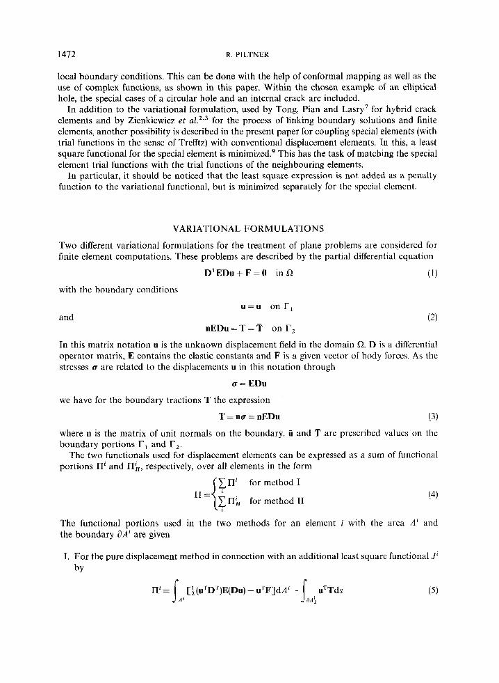
I. For the pure displacement method in connection with an additional least square functional J' by

[f(uTDT)E(Du) - uTF]dAi - ( 5 )

SPECIAL FINITE ELEMENTS 1473

and J L j (ii - ~ ) ~ ( i i - u)ds = minimum for element i (6)

8,4; ta.4;

and 11. for the hybrid displacement method (based on an extended functional for the potential energy)

by

TT(ii - u)ds (7) s 3A; + a A ;

n+ni+

The boundary dA' of an element consists of three parts:

dA' = dA\ + 8A; + dA\

where dAi c rl, dAL c rZ and 8Ai is the inter-element boundary. ii is a vector of independently assumed boundary displacements, which are the same for two adjacent elements over their common boundary. For the special elements, the displacement field u is chosen for the element domain in such a way that the system of differential equations (1) and local boundary conditions are a priori satisfied. T is chosen according to relation (3).

It should be noted that the least square functional J' can be minimized separately for each element. As J' is not added to H i as a penalty function, the problem of finding an optimal factor for the penalty term does not arise. The result of the minimization of J' is an optimal relationship between free parameters and nodal values, which is substituted in ni for method 1. Using the hybrid functional (method II), the determination of the relationship between parameters and nodal values is realized with the extension term ITT@ - u)ds. One essential difference between the two methods is that there must be rigid body terms in method I, whereas in method I1 no rigid body terms are allowed.

Assuming the special trial functions in a proper way, we distinguish a homogeneous solution part uh and a particular part up, where only the homogeneous part has free parameters. So the displacement field can be expressed in the form

u = up + uh,

whereas the according boundary tractions T can be formulated with a homogeneous part T, = nEDu, and a particular part T, = nEDu, as

(9)

By reason of the solution properties of the trial functions, the expression nL of relation ( 5 ) and (7) can be simplified to the following form with boundary integral expressions:

(8)

T = T, + T,

$u;fT,ds + J ugT,ds - J ugTds + terms without u h and T, ni = J a,i 3.4' 8.4; (10)

Since only the homogeneous solution part contains free parameters, all terms of II' not involving uh and T, are of no significance for an approximate solution and are therefore not listed explicitly.

The decomposition into a homogeneous and a particular part is done not only with regard to the satisfaction of the homogeneous and inhomogeneous differential equation, but also in view of the exact fulfilment of homogeneous and inhomogeneous boundary conditions on some portions of the element boundary, for example on the surface of a circular hole. For the special elements, we assume that displacement boundary conditions u = U on 8A i are satisfied in the form

U , = O ondA\

1474 R. PILTNER

and

whereas

and

are suitable conditions for the fulfilment of traction boundary conditions T = T on aA',. In these cases and if the boundary portions aA1 and aA; , respectively, do not belong to the element boundary, one needs only to integrate on the inter-element boundary aAI;.

STIFFNESS MATRICES AND LOAD VECTORS FOR SPECIAL ELEMENTS

The displacement field with the components u and u can be expressed in matrix form as

and UP = [;;I Uh = [3

where c are the unknown parameters. Analogously, the boundary tractions with the components Tx and T, can be written as

and (14)

The assumed functions ii on the inter-element boundary are chosen to be linear or quadratic according to the choice of the conventional (iso- and subparametric) adjacent elements. They can be expressed with two vectors 0 and v, which contain one-dimensional shape functions, and with the nodal displacements q in the following form:

ii=[;]=[O D o v]q

For example, in the case of linear boundary displacements between two nodes p and p + 1

i & t I

P P+ l

t AXl l-+4-+A

P P+l P+Z

I---l---I l--l---I (a) (b)

Figure 1. Special elements with elliptical holes: (a) 8-node element with linear ii between nodes p and p + 1, (b) 16-node element with quadratic ii between nodes p and p + 2

SPECIAL FINITE ELEMENTS 1475

(Figure 1) with nodal values (up, up) and (up+ u p + we have

and

1 is the distance between the two nodes, and s represents a boundary co-ordinate, which is measured from node p . After substituting the terms explained above into (5) and (6) one gets for method I

and

where

Hi = fcTHc + cTrl + terms without c

J ' = fc'Qc - cTf;q + cTrZ + terms without c and q

H = { $[UTT, + T;U + VTT, + TFVlds

Q = 1 [UTU + VTV]ds

8.43

aA3

r

r, = J [UTTxp + VTTyp]ds aA:

r2 = j [UTu, + VTup]ds 8A:

For the hybrid functional of method I1 we obtain

l3& = - &cTHc + cTLq - cTr3 + qTr, + terms without c and q (21)

r3 = 1 [T:u, + TFu,]ds an;

r 4 = [la(O'Txpd]

TTTJpds

The expression for H according to equation (19) is valid here also. The only difference is in computing the H matrices for methods I and I1 and lies in the presence or absence of rigid-body terms.

In both methods we look for an optimal relationship between c and q in the sense of the process

1476 R. PILTNER

used. This relationship can be expressed with a matrix G and a row vector g in the general form

c = c q + g (23) The optimal connection of c and q is gotten for method I from

Z q + r z = O

whereas for the hybrid method the defining equation for c is obtained from

ang aCT -= -Hc+Lq-rr ,=O

Using the general form for c, we can get rather similar expressions for ni and IIk; in fact from (17) and (21) we obtain

ni = 3qTGTHGq + qT[GTHg + GTr,] + terms without q (26)

(27) and n g - 1 T - z q CTHGq + qT[GTHg + r4] + terms without q

Taking into consideration the different meanings of G and g for the two methods (G = Q-'Z, g = - Q- 'r2 for method I and G = H - 'L, g = - H- 'r3 for method 11), one obtains the element- stiffness matrix k and the load vector p for method I in the form

k = GTHG = (ETQ-')H(Q-'E), p = -GTIHg+r l l = -(~'Q-')[H(-Q-'r2)+r,]

(28)

and for method I1 in the form

k = GTHG = LTH-'HH-'L = LTH-'L p = - GTHg - r4 = - (LTH-' )H( - H-'r3) - r4 = LTH-'r3 - r4 (29)

CONSTRUCTION OF SPECIAL TRIAL FUNCTIONS

The best way of constructing special trial functions seems to be to start at a formulation with functions of a complex variable z = x + iy. Using two analytic functions 4 ( z ) and $(z) we can express the displacements and stresses in the form'

_ _ ~ 2/44 + iu) = K&Z) - z 4 ' ( z ) - $ ( z )

crXx + irxy = # ( z ) + # ( z ) - Z$"(Z) - $'(z)

5yy - i Z X Y = # ( z ) + &(z) + z(b"(z) + $'(z)

_ _ _ _ _ _ _ (30)

_ _ _ ~ _ _ _

where p = E/2(1 + v) and K = (3 - v)/(l + v) for plane stress and K = 3 - 4v for plane strain. ( )' denotes complex differentiation with respect to z and (-) denotes the complex conjugate. In complex form, the boundary conditions are

and

_ _ _ _ .+(z) - z # ( z ) - $(z) = 2p(U + iU) on rl

n

4 ( z ) + z @ ( z ) + $(z) = i (Tx + iTy)ds on Tz ~- ~ J

As the treatment of boundary conditions in the original domain usually fails, it is convenient and

SPECIAL FINITE ELEMENTS 1477

I- a -4

= rcr;, t - plane 5 - plane

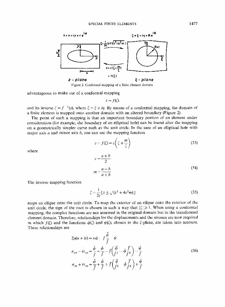
Figure 2. Conformal mapping of a finite element domain

advantageous to make use of a conformal mapping

z = f (i) and its inverse i = j - ‘ ( z ) , where i = < + ir]. By means of a conformal mapping, the domain of a finite element is mapped onto another domain with an altered boundary (Figure 2).

The point of such a mapping is that an important boundary portion of an element under consideration (for example, the boundary of an elliptical hole) can be found after the mapping on a geometrically simpler curve such as the unit circle. In the case of an elliptical hole with major axis a and minor axis h, one can use the mapping function

where

a - h a + h

ni = (34)

The inverse mapping function

(35) 1

2c [ = -[z f d ( Z 2 + 4c2rn)l

maps an ellipse onto the unit circle. To map the exterior of an ellipse onto the exterior of the unit circle, the sign of the root is chosen in such a way that [[I3 1. When using a conformal mapping, the complex functions are not assumed in the original domain but in the transformed element domain. Therefore, relationships for the displacements and the stresses are now required in which f ( 5 ) and the functions $([) and $([), chosen in the [-plane, are taken into account. These relationships are

6 - 2p(u + iv) = rc$ - f--; - $

f ’

1478 R. PILTNER

( . ) denotes complex differentiation with respect to <. The transformed boundary conditions for the new curves, denoted r; and rl,, can be expressed in the following manner:

4 ~ _ _ $([) = K$ - fT - 2p(u + iV) f

on r; (37)

Since $(5) must be an analytic function, the right-hand sides of the boundary ___ ~ equations (37) and (38) must also be analytic. However, the conjugate complex terms 4([), f(i), etc., are not normally analytic functions. The problem in satisfying the boundary conditions is therefore to search for analytic functions, which agree on the curves r; or r; with the non-analytic functions on the right-hand sides of (37) and (38). In treatment of this problem with a conformal mapping onto a unit circle, the important relationshipt

-

y=[-" on 1[1=1 (39)

can be used to advantage, where CI is real. One important step in satisfying boundary conditions is the splitting of the boundary values

into homogeneous and inhomogeneous parts, as in equations (11) and (12). The strategy in satisfying a boundary condition through a suitable construction of a function $ includes the following points:

1. Choose 4(i) as a complex power series. 2. Approximate j ( [ ) with a power series, i f f is not a priori expressed as a polynomial in [. 3. Express (U + iV) and l (Tx + iT,)ds as polynomials in [ in the case of inhomogeneous boundary

4. Replace the conjugate complex function terms by analytic expressions using (39).

The choice of +(i) for an element with an elliptical hole is made in the form of a complex Laurent series

conditions.

with complex coefficients uj = cl j + iBj. Now on the unit circle the following equations are valid:

With the help of equations (40) to (42) we at once obtain the unknown function II/ for homogeneous boundary conditions from (37) and (38), respectively. For the example of a homogeneous stress boundary condition (T, = Ty = 0 on the boundary of an elliptical hole), we obtain

which in connection with 4 from equation (40) enables us to compute the displacements and -

'Corresponding relationships for a mapping on a half-plane are ( j = [ j on the real axis and axis, where j is an integer.

= ( - l)j(j on the imaginary

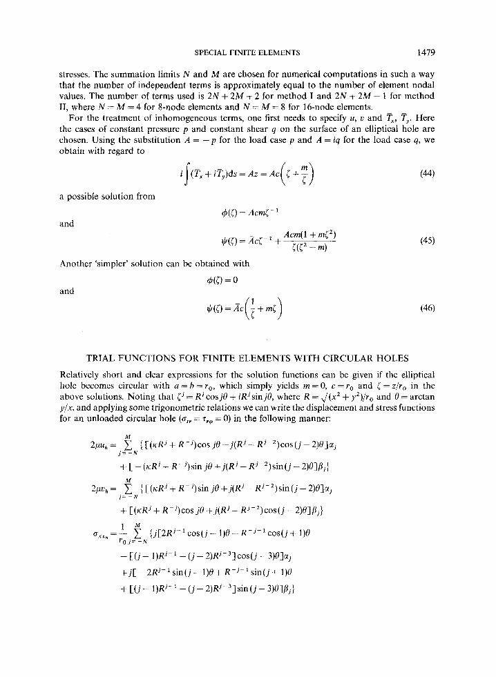
SPECIAL FINITE ELEMENTS 1479

stresses. The summation limits N and M are chosen for numerical computations in such a way that the number of independent terms is approximately equal to the number of element nodal values. The number of terms used is 2N + 2M + 2 for method I and 2N + 2M - 1 for method 11, where N = M = 4 for 8-node elements and N = M = 8 for 16-node elements.

For the treatment of inhomogeneous terms, one first needs to specify U, 17 and Tx, Ty. Here the cases of constant pressure p and constant shear q on the surface of an elliptical hole are chosen. Using the substitution A = - p for the load case p and A = iq for the load case q, we obtain with regard to

i (Tx+iTy)ds=Az=Ac s a possible solution from

and

(44)

Another 'simpler' solution can be obtained with

TRIAL FUNCTIONS FOR FINITE ELEMENTS WITH CIRCULAR HOLES

Relatively short and clear expressions for the solution functions can be given if the elliptical hole becomes circular with a = b = r , , which simply yields m = 0 , c=ro and [ =z/ro in the above solutions. Noting that {j = Rj cos j0 + iRjsin j0, where R = J(xz + y 2 ) / r , and 8 = arctan y/x, and applying some trigonometric relations we can write the displacement and stress functions for an unloaded circular hole (err = zr, = 0) in the following manner:

M

2pu, = c { [I ( K R ~ + R-j)cos j0 - j (Rj - Rj- ')cos ( j - 2)O]gj i= - N

+ [ - ( ~ R j + R - j ) s i n jO+j(Rj-RRj-2)sin(j-2)8],8j}

2pv,= c {[(K-Rj+R-j)sin j O + j ( R j - R j - 2 ) s i n ( j - 2 ) 0 ] a j M

j = - N

+ [ ( I & + R-j)cosjO+j(Rj- Rj-2)cos(j-2)O]/?j}

l M uXXh =-- c {.j[2Rj-'cos(j- l)8- R-j- 'cos( j + 1)0 r,j= - N

- [ C j - 1)RJ-' -(j-2)Rj-3]cos(j-3)H]aj

+j[-2RJ- 's in( j - 1)8+ R-j- ' s in( j+ l)8

+ [(j - 1)Rj-I - ( j - 2)RjP3] sin ( j - 3)8]pj}

1480 R. PILTNER

1 M

+[(j- 1)Rj-I - ( j -2)Rj-3]c~s( j -3)0]aj

+ j[ - 2Rj- ' sin( j - 1)0 - R - j - ' sin(j + 1)8

- [(j- 1)Rj-l -(j-2)Rj-3]sin(j-3)0]bj}

1 M

ro j = - N z X Y h = - 1 ( j [ -R-J- ' s in( j+ l)O+[(j- l ) R j - 1 - ( , j - 2 ) R j - 3 ] s i n ( j - 3 ) 0 ] a j

+j[ -R- j - ' cos( j+ 1)0+[( j - 1)Rj-I -(j-2)Rj-3] cos(j-3)t)]/l,j} (47)

With these functions the required homogeneous vectors uf = [UcVc] = [u,,vJ and TT =

[T,c T,cl= C(oxxhnx + z,yhny)(oyyhny + zxYhnx)] can be given listing the free parameters aj and Dj as a vector cT = [aTBT].

For the boundary condition orr = - p on the surface of a circular hole, we obtain the following expressions:

2puP = pr,R- cos 0 2pv, = pr,R-' sin 0

(T,~, = p R - 2 cos 20 zxy,= - ~ R - ~ s i n 2 8

oXx, = - pR- cos 20 (48)

which can be used to obtain the particular vectors u f = [u,v,] and T;S= [TxPTyI7] =

[ ( C J , ~ , ~ ~ + z,y,ny)(oyy,ny + z,,,n,)]. Analogously, the concrete solution terms for the boundary condition T~~ = q are

2pu, = - qroR-' sin 8 2pv, = - qr,R ' cos 0 oxxl, = - q R - sin 20 oYYp = q R - sin 20 zxy, = qR-2 cos 20

(49)

STRESS CONCENTRATION FACTORS FOR ELEMENTS WITH INTERNAL. CRACKS

If the elliptical hole degenerates to a slit the stresses become singular at the two crack tip points. Since also for internal cracks the stresses in the vicinity of crack tip points are of the form l/,/r' (r' = radius around a crack tip point), it is possible to determine stress concentration factors. For the two crack tip points z = a and z = - a (Figure 3), located at [ = 1 and [ = - 1 in the transformed plane, we obtain9,' I t

( 50)

Often in the literature a factor J n is used in the definition of stress intensity factors. In these cases, the right-hand side of (50) is to be multiplied by 4..

SPECIAL FINITE ELEMENTS 1481

- Figure 3. Internal crack element with quadratic

NUMERICAL EXAMPLES

To investigate the accuracy of the special elements, some examples have been chosen for which exact solutions are known. Besides the special elements, conventional displacement elements are used. For the computations with assumed plane stress, the values E = 1, v = 0.3, p = 1 have been chosen.

Infinite plate with a circular hole under normal tension

This plate is idealized by a finite element model according to Figure 4. The results agree fairly well with the analytic solution containing the stress tips oVg = 3 p in a horizontal cut and og9 = - p in a vertical cut (Table I). Using elements with quadratic ii, one can scarcely see differences in the results between method 1 and method IT.

t t t t t t t l t l t t t t t t t t t t t P 14

14

12

10

10

12

14

14

1 1 1 1 1 1 1 1 1 1 1 1 1 1 1 1 II l l l p I- -:- p

14 14 12 10 10 12 14 14

Figure4. Finite element model for an infinite plate with a cicular hole (1 special element, 60 conventional displacement elements)

1482 R. PILTNER

Table I. Errors for I c T , , , ~ ~ ~ ~ ~ in per cent

In a horizontal cut In a vertical cut Method I Method I1 Method I Method I1

Linear a: 1.3 0.2 2.1 0.5 Quadratic 5: 0.3 0.3 0 6 0.7

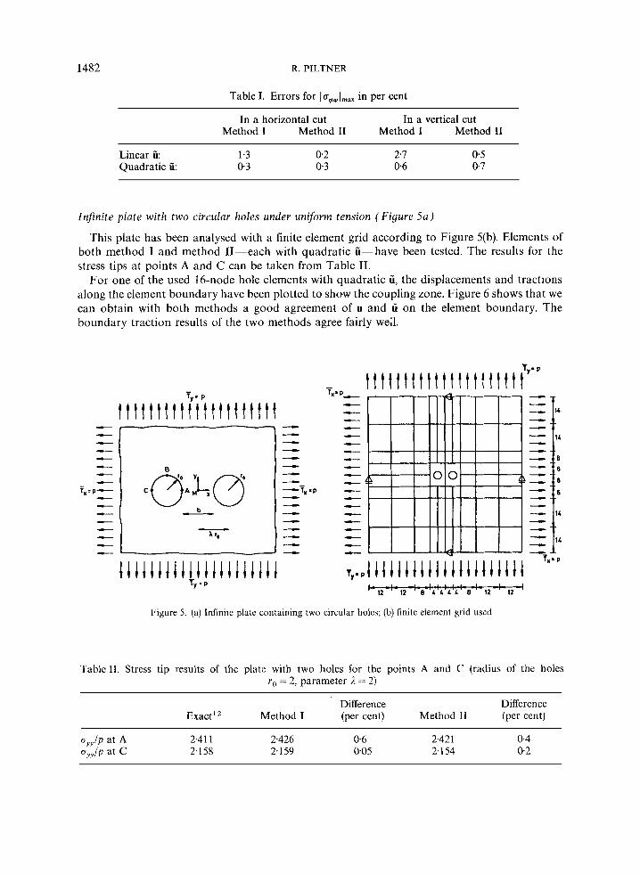
Infinite plate with two circular holes under ungorm tension (Figure 5a)

This plate has been analysed with a finite element grid according to Figure 5(b). Elements of both method I and method IT--each with quadratic Q-have been tested. The results for the stress tips at points A and C can be taken from Table IT.

For one of the used 16-node hole elements with quadratic ii, the displacements and tractions along the element boundary have been plotted to show the coupling zone. Figure 6 shows that we can obtain with both methods a good agreement of u and ii on the element boundary. The boundary traction results of the two methods agree fairly weJ.

- t t t t t t t t t t t t t t t t t I t t il” -

t t t f t t t t t i’ii t t t t t t t t t

ll1llil11lllilllll1l1 r, = ?

‘X’?,

c c c c c c c c c c c c c c c c c c c c

T 14

14

6

6

6

6

14

14

-

Figure 5. (a) Infinitc plate containing two circular holcs; (b) finite element grid used

TableII. Stress tip results of the plate with two holes for the points A and C (radius of the holes ro = 2, parameter 1 = 2)

Difference Difference ExactI2 Method I (per cent) Method I1 (per cent)

“ y y l P at A 2.41 1 2.426 0.6 2.42 1 0.4 “ y y l P at c 2.1 58 2.159 0.05 2.1 54 0.2

SPECIAL FINITE ELEMENTS 1483

Howland strip of width 2b = 20 containing a hole ojradius ro = 2

This strip has been idealized through a finite element grid according to Figure 7. Finite elements with quadratic ii yielded stress-tip values (Table 111), which agree fairly well with the exact values.

t t t t t t t t t t t ’ 6

6

, 8

0

6

6

I--r----t-----c-l 25 7.5 7.5 25

Figure 7. Finite element grid for a Howland strip

1484 R. PILTNER

Table 111. Stress tip results for a Howland strip at points A and B (radius of the hole ro = 2, ro/b = 0.2)

Difference Difference Exact' Method I (per cent) Method I1 (per cent)

oqq/p at A 3.14 3.141 0.03 3.145 0.16 gqOlp at B - 1.1 1 - 1.114 0.4 - 1.1 14 0.4

t t t t t t t t t t t t t t t t t p = '

e x a c t :

K1 = 1.414 Kl = 1.414

1

e x a c t :

K1 = 1.414 Kl = 1.414

1

I 1

I1 I I 1 1 I I I1 I1 1 1 I I I p = '

1L

14

12

10

10

12

14

14

(b) '14 ' 14 %? 10 ' 10+12 ' 14- I ,

Figure 8. (a) Infinite plate with an internal crack; (b) finite element grid with 60 conventional displacement elements and 1 special element containing an internal crack

Internal crack of length 2a = 4 in an infinite plate under tension (Figure 8)

For the study of this plate, a finite element grid with 60 conventional elements and one special internal-crack element has been used. The use of elements with linear varying boundary displacements ii yielded K , = 1.399 for method I and K , = 1.412 for method 11. Using elements with quadratic ii, one can scarcely observe a difference between the two methods; we have K 1 = 1.4165 for method I and K , = 1.4164 for method 11. In all numerical computations, K , was of the order of So in all cases the results agree very well with the exact values K , = 1.414 and K,=O.

CONCLUSIONS

Using independently assumed boundary displacements, the coupling of special problem-adapted elements with conventional displacement elements can be realized almost equally effectively in two different ways. The basic equations of the two methods are compared. A systematology for the derivation of special problem-adapted trial functions has been illustrated using the example of elements with holes and internal cracks. One advantage of the special elements is that the stiffness matrices can be evaluated via simple numerical integrations along the inter-element

SPECIAL FINITE ELEMENTS 1485

boundaries. Numerical examples showed that rather good results can be obtained with geornetri- cally simple finite element grids.

REFERENCES

1. E. Trefftz, ‘Ein Gegenstuck zum Ritzschen Verfahren’, 2. Int. Kongr. fur Techn. Mech., Zurich, 1926, pp. 131-137. 2. 0. C. Zienkiewicz, D. W. Kelly and P. Bettess, ‘The coupling of the finite element method and boundary solution

procedure’, Int. j . numer. methods eng., 11, 355-375 (1977). 3. 0. C. Zienkiewicz, D. W. Kelly and P. Bettess, ‘Marriage a la mode-the best of both worlds (finite elements and

boundary integrals)’, Proc. Int. Symp. on Innovative Numerical Analysis in Applied Engineering Science, Versailles, May 1977, pp. 19-26. Also, Ch. 5, pp. 81-106 in Energy Methods in Finite Element Analysis (Eds. R. Glowinski, E. Y. Rodin and 0. C. Zienkiewicz), Wiley, New York, 1979.

4. 0. C . Zienkiewicz, ‘The Finite Element Method’, 3rd edn, McGraw-Hill, London 1977. 5. T. H. H. Pian, ‘Derivation of element stiffness matrices by assumed stress distribution’, A.I.A.A. J . , 2 (7), 1333-1336

6. E. Byskov, ‘The calculation of stress intensity factors using the finite element method with cracked elements’, Int. J .

7. P. Tong, T. H. H. Pian and S. Lasry, ‘A hybrid element approach to crack problems in plane elasticity’, Int. j . numer.

8. K. Y. Lin and P. Tong, ‘Singular finite elements for the fracture analysis of V-notched plate’, Int. j . numer. methods eng.,

9. R. Piltner, ‘Spezielle finite Elemente mit Lochern, Ecken und Rissen unter Verwendung von analytischen Teillosungen’, Doctoral thesis, Ruhr-Universitat Bochum, Fortschr.-Ber. VDI-Z. Reihe 1 Nr. 96, VDI-Verlag, Diisseldorf, 1982.

10. N. I. Muskhelishvili, ‘Some Basic Problems of the Mathematical Theory ofElasticity’, Noordhoff, Groningen, Holland, 1953.

11. G. C. Sih, P. C. Paris and F. Erdogan, ‘Crack-tip stress-intensity factors for plane extension and plate bending problems’, J . Appl . Mech., 29, 306-312 (1962).

12. G. N. Sawin, Spannungserhiihungen am Rande uon Lochern, VEB-Verlag Technik, Berlin, 1956, pp. 150-154. 13. R.C. J. Howland, ‘On the stresses in the neighbourhood of a circular hole in a strip under tension’, Phil. Trans. Roy. SOC.,

(1964).

Fract. Mech., 6, 159-167 (1970).

methods eng., 7 , 297-308 (1973).

15, 1343-1354 (1980).

London, A229,49-86 (1930).