THE ASYMPTOTIC CRITICAL WAVE SPEED IN A FAMILY OF SCALAR

REACTION-DIFFUSION EQUATIONS

FREDDY DUMORTIER, NIKOLA POPOVIC, AND TASSO J. KAPER

Abstract. We study traveling wave solutions for the class of scalar reaction-diffusion equations

∂u

∂t=

∂2u

∂x2+ fm(u),

where the family of potential functions fm is given by fm(u) = 2um(1 − u). For each m ≥ 1real, there is a critical wave speed ccrit(m) that separates waves of exponential structure from thosewhich decay only algebraically. We derive a rigorous asymptotic expansion for ccrit(m) in the limitas m → ∞. This expansion also seems to provide a useful approximation to ccrit(m) over a widerange of m-values. Moreover, we prove that ccrit(m) is C∞-smooth as a function of m−1. Ouranalysis relies on geometric singular perturbation theory, as well as on the blow-up technique, andconfirms the results obtained by means of asymptotic methods in [D.J. Needham and A.N. Barnes,Nonlinearity, 12(1):41-58, 1999] and in [T.P. Witelski, K. Ono, and T.J. Kaper, Appl. Math. Lett.,14(1):65-73, 2001].

1. Introduction

We consider traveling wave solutions for the class of scalar bistable reaction-diffusion equationsgiven by

∂u

∂t=∂2u

∂x2+ fm(u),(1)

where the family of potential functions fm is defined via fm(u) = 2um(1 − u), with m ≥ 1 real.The restriction to m ≥ 1 is necessary, since it has been shown in [17, 27] that no traveling wavesfor (1) can exist when m < 1, see also [21].

The class of problems in (1) includes the classical Fisher-Kolmogorov-Petrowskii-Piscounov(FKPP) equation with quadratic nonlinearity (m = 1) [10, 12], as well as a bistable equationwith degenerate cubic nonlinearity (m = 2) [25]. In particular, it has been studied in [25] as abridge between the classical FKPP equation and the family of nondegenerate bistable cubic equa-tions with potential f(u) = u(u−a)(1−u), a ∈ (0, 1

2). In the former, u = 0 is an unstable state (inthe PDE sense), whereas in the latter, it is a stable state of the PDE. The motivation for studying(1) in [25] was that it is a family of equations for which the state u = 0 is neutrally stable and, hence,that it lies “in between” the two classical cases. Interesting mathematical phenomena concerningthe stability of wave fronts were reported in [25], see also [18, 15]. We hope that the existenceanalysis presented here will be useful for further investigating the stability of these solutions.

Let the traveling wave solutions to (1) be denoted by u(x, t) = U(ξ), with ξ = x−ct the travelingwave variable and c the wave speed. Moreover, let

limξ→∞

U(ξ) = 0 and limξ→−∞

U(ξ) = 1.

Date: November 29, 2006.1991 Mathematics Subject Classification. 35K57, 34E15, 34E05.Key words and phrases. Reaction-diffusion equations; Traveling waves; Critical wave speeds; Asymptotic expan-

sions; Blow-up technique.

1

It is well-known that for each m ≥ 1, there is a critical wave speed ccrit(m) > 0 such that travelingwave solutions exist for c ≥ ccrit(m) in (1) [2, 1]. The speed ccrit(m) is critical in the sense thatwaves decay exponentially ahead of the wave front (i.e., as ξ → ∞) when c = ccrit(m), whereas thedecay is merely algebraic in ξ for c > ccrit(m).

The family of equations in (1) has been studied in the regimes where m is near 1 or 2. Perturba-tion analyses off these classical cases have been carried out for m = 1+ε using matched asymptoticexpansions [17] and geometric singular perturbation theory [21], showing that the limit as ε→ 0 isnon-uniform, with the critical wave speed given by

ccrit(1 + ε) = 2√

2 −√

2Ω0ε2

3 + O(ε) for ε ∈ (0, ε0).

Here, ε0 > 0 is small, and Ω0 is the first real zero of the Airy function. The corresponding resultfor m ≈ 2 is

ccrit(2 + ε) = 1 − 13

24ε+ O(ε2) for ε ∈ (−ε0, ε0),

see also [27].In the following, we study (3) in the limit of m → ∞. This problem was considered in [27]

via the method of matched asymptotic expansions; independently, it was analyzed in [18] using aslightly different approach. In particular, it has been shown that ccrit(m) ∼ 2

mto leading order for

the critical wave speed ccrit that separates solutions in (1) which decay exponentially from thosefor which the decay is merely algebraic.

Here, the aim is to derive a rigorous asymptotic expansion for ccrit(m) in the large-m limit, andthereby to justify the matched asymptotic analysis of [27] and [18] within a geometric framework.At the same time, we will also obtain an alternative proof for the existence of the correspondingtraveling wave solutions in (1). Two additional factors motivated the analysis of the large-m limit.First, both the asymptotic analysis and the numerical results in [27, 18] suggest that ccrit(m)decreases monotonically to zero as m→ ∞, which is confirmed in Theorem 1.1 below. Second, theexpansion for ccrit(m) as m→ ∞ agrees well with the numerics over a wide range of m-values, evendown to m = 2, see [27, Figure 3(a)]. Hence, the results obtained in the large-m regime seem toprovide a useful approximation to ccrit(m) also for finite values of m.

The following is the principal result of this work:

Theorem 1.1. There exists a function ccrit(m) and an m0 ∈ R sufficiently large such that form ≥ m0, c = ccrit(m) is the critical wave speed for (1). Moreover, ccrit(m) is C∞-smooth in m−1,and there holds

ccrit(m) =2

m+

σ

m2+ O(m−3),(2)

where σ is defined as

σ = limω0→∞

∫ ω0

0

[ω2e−ω

√1 − (1 + ω)e−ω

− ω3

2e−ω

]dω ≈ −0.3119.

The main technique we use to prove Theorem 1.1 is the global blow-up technique, also known asgeometric desingularization of families of vector fields. To the best of our knowledge, this methodwas first used in studying the limit cycles near a cuspidal loop in [7]. The blow-up technique hassince been successfully applied in the study of numerous bifurcation problems. It has for instancebeen introduced in [5] as an extension of the more classical geometric singular perturbation theory[9, 11] to problems in which normal hyperbolicity is lost. For further examples, we refer the readerto [3, 6, 4, 13, 14, 22].

2

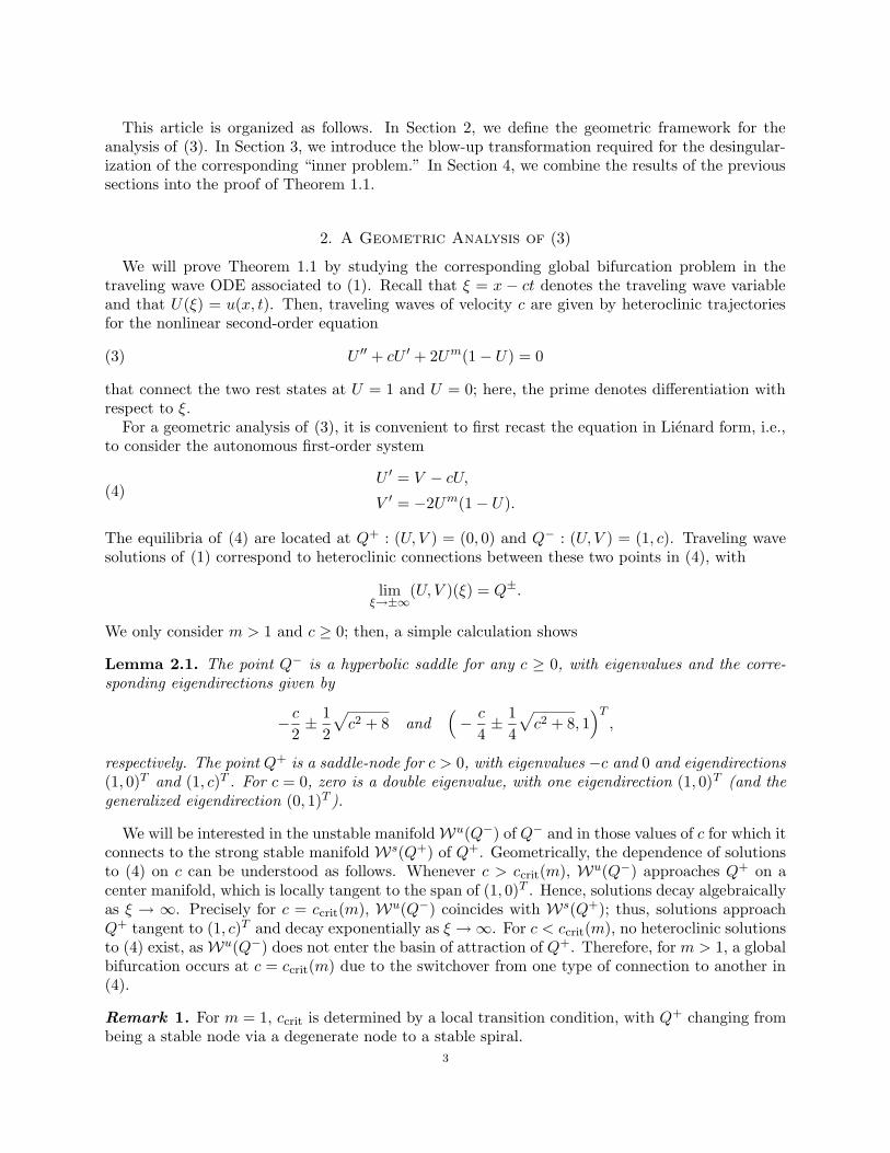
This article is organized as follows. In Section 2, we define the geometric framework for theanalysis of (3). In Section 3, we introduce the blow-up transformation required for the desingular-ization of the corresponding “inner problem.” In Section 4, we combine the results of the previoussections into the proof of Theorem 1.1.

2. A Geometric Analysis of (3)

We will prove Theorem 1.1 by studying the corresponding global bifurcation problem in thetraveling wave ODE associated to (1). Recall that ξ = x − ct denotes the traveling wave variableand that U(ξ) = u(x, t). Then, traveling waves of velocity c are given by heteroclinic trajectoriesfor the nonlinear second-order equation

U ′′ + cU ′ + 2Um(1 − U) = 0(3)

that connect the two rest states at U = 1 and U = 0; here, the prime denotes differentiation withrespect to ξ.

For a geometric analysis of (3), it is convenient to first recast the equation in Lienard form, i.e.,to consider the autonomous first-order system

U ′ = V − cU,

V ′ = −2Um(1 − U).(4)

The equilibria of (4) are located at Q+ : (U, V ) = (0, 0) and Q− : (U, V ) = (1, c). Traveling wavesolutions of (1) correspond to heteroclinic connections between these two points in (4), with

limξ→±∞

(U, V )(ξ) = Q±.

We only consider m > 1 and c ≥ 0; then, a simple calculation shows

Lemma 2.1. The point Q− is a hyperbolic saddle for any c ≥ 0, with eigenvalues and the corre-sponding eigendirections given by

− c2± 1

2

√c2 + 8 and

(− c

4± 1

4

√c2 + 8, 1

)T

,

respectively. The point Q+ is a saddle-node for c > 0, with eigenvalues −c and 0 and eigendirections(1, 0)T and (1, c)T . For c = 0, zero is a double eigenvalue, with one eigendirection (1, 0)T (and thegeneralized eigendirection (0, 1)T ).

We will be interested in the unstable manifold Wu(Q−) of Q− and in those values of c for which itconnects to the strong stable manifold Ws(Q+) of Q+. Geometrically, the dependence of solutionsto (4) on c can be understood as follows. Whenever c > ccrit(m), Wu(Q−) approaches Q+ on acenter manifold, which is locally tangent to the span of (1, 0)T . Hence, solutions decay algebraicallyas ξ → ∞. Precisely for c = ccrit(m), Wu(Q−) coincides with Ws(Q+); thus, solutions approachQ+ tangent to (1, c)T and decay exponentially as ξ → ∞. For c < ccrit(m), no heteroclinic solutionsto (4) exist, as Wu(Q−) does not enter the basin of attraction of Q+. Therefore, for m > 1, a globalbifurcation occurs at c = ccrit(m) due to the switchover from one type of connection to another in(4).

Remark 1. For m = 1, ccrit is determined by a local transition condition, with Q+ changing frombeing a stable node via a degenerate node to a stable spiral.

3

2.1. A preliminary rescaling for (4). We define the new parameter ε = m−1 and hence considerthe limit of ε→ 0 in the following. Given that the function fm(U) assumes its maximum at U = m

m+1and that

fm( mm+1) = 2

( m

m+ 1

)m 1

m+ 1∼ 2

eε

for m sufficiently large, we rescale V via V = εV . Also, we know formally and numerically thatccrit = O(1) as ε→ 0 [18, 27]; therefore, we write c = εc.

Under these rescalings, the equations in (4) become

U = V − cU,(5a)

˙V = − 2

ε2U

1

ε (1 − U);(5b)

here, the overdot denotes differentiation with respect to the rescaled traveling wave coordinate

ξ = εξ.(6)

We investigate (5) in the limit as ε → 0. More precisely, we will decompose the analysis of(5) into two separate problems, the “outer problem” and the “inner problem,” which are definedfor 0 ≤ U < 1 and for U ≈ 1, respectively. This decomposition is naturally suggested when one

introduces U1

ε = e1

εln U in (5b), since this term is exponentially small if U < 1. The desired

expansion for ccrit(ε) will then be obtained by constructing a solution which is uniformly valid onthe entire domain [0, 1].

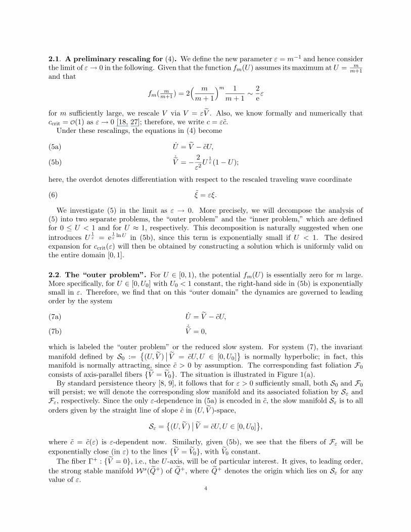
2.2. The “outer problem”. For U ∈ [0, 1), the potential fm(U) is essentially zero for m large.More specifically, for U ∈ [0, U0] with U0 < 1 constant, the right-hand side in (5b) is exponentiallysmall in ε. Therefore, we find that on this “outer domain” the dynamics are governed to leadingorder by the system

U = V − cU,(7a)

˙V = 0,(7b)

which is labeled the “outer problem” or the reduced slow system. For system (7), the invariant

manifold defined by S0 :=(U, V )

∣∣ V = cU, U ∈ [0, U0]

is normally hyperbolic; in fact, thismanifold is normally attracting, since c > 0 by assumption. The corresponding fast foliation F0

consists of axis-parallel fibers V = V0. The situation is illustrated in Figure 1(a).By standard persistence theory [8, 9], it follows that for ε > 0 sufficiently small, both S0 and F0

will persist; we will denote the corresponding slow manifold and its associated foliation by Sε andFε, respectively. Since the only ε-dependence in (5a) is encoded in c, the slow manifold Sε is to all

orders given by the straight line of slope c in (U, V )-space,

Sε =(U, V )

∣∣ V = cU, U ∈ [0, U0],

where c = c(ε) is ε-dependent now. Similarly, given (5b), we see that the fibers of Fε will be

exponentially close (in ε) to the lines V = V0, with V0 constant.

The fiber Γ+ : V = 0, i.e., the U -axis, will be of particular interest. It gives, to leading order,

the strong stable manifold Ws(Q+) of Q+, where Q+ denotes the origin which lies on Sε for anyvalue of ε.

4

U0 1

S0 : V = cU

Q+

Q−

Γ+

V

U

(a) The “outer problem” (7).

W01Q−

S0 : Z = cW

Q+

Γ−

Z

W

(b) The “inner problem” (10).

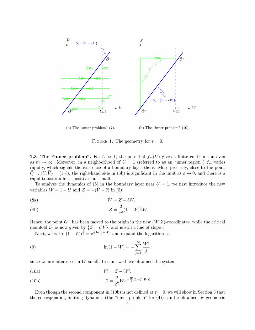
Figure 1. The geometry for ε = 0.

2.3. The “inner problem”. For U ≈ 1, the potential fm(U) gives a finite contribution evenas m → ∞. Moreover, in a neighborhood of U = 1 (referred to as an “inner region”) fm variesrapidly, which signals the existence of a boundary layer there. More precisely, close to the point

Q− : (U, V ) = (1, c), the right-hand side in (5b) is significant in the limit as ε → 0, and there is arapid transition for ε positive, but small.

To analyze the dynamics of (5) in the boundary layer near U = 1, we first introduce the new

variables W = 1 − U and Z = −(V − c) in (5):

W = Z − cW,(8a)

Z =2

ε2(1 −W )

1

εW.(8b)

Hence, the point Q− has been moved to the origin in the new (W,Z)-coordinates, while the criticalmanifold S0 is now given by Z = cW, and is still a line of slope c.

Next, we write (1 −W )1

ε = e1

εln (1−W ) and expand the logarithm as

ln (1 −W ) = −∞∑

j=1

W j

j,(9)

since we are interested in W small. In sum, we have obtained the system

W = Z − cW,(10a)

Z =2

ε2W e−

Wε

(1+O(W )).(10b)

Even though the second component in (10b) is not defined at ε = 0, we will show in Section 3 thatthe corresponding limiting dynamics (the “inner problem” for (4)) can be obtained by geometric

5

desingularization (blow-up) [3]. In particular, the inner limit of (10b) as (W, ε) → (0, 0) is non-uniform. Heuristically, the limiting dynamics for ε→ 0 should be described by the singular orbit

Γ− :=(0, Z)

∣∣Z ∈ [0, c]∪

(W, c)

∣∣W ∈ [0,W0],(11)

where W0 = 1 − U0 (with U0 defined as above). The orbit Γ− consists of that portion of theZ-axis which to lowest order describes the boundary layer at W = 0, as well as of a segment of

Z = c which corresponds to the fiber V = 0 in the “outer” coordinates, see Figure 1(b). Thisintuition will be made rigorous using geometric desingularization to analyze the dynamics of (10)in a neighborhood of the Z-axis.

3. The blow-up transformation for (10)

To desingularize the dynamics of (10) close to the Z-axis, we define the cylindrical blow-uptransformation

W = rw, Z = z, ε = rε,(12)

where (w, ε) ∈ S1+ =

(w, ε)

∣∣ w2 + ε2 = 1, w, ε ≥ 0, z ∈ [0, z0], and r ∈ [0, r0].

Remark 2. The central idea underlying the blow-up technique is to rescale both phase variablesand parameters in a manner that transforms a non-hyperbolic situation into a hyperbolic one, withfixed points (respectively lines of non-isolated fixed points) typically being blown-up into spheres(respectively cylinders). Mathematically, an n-dimensional equation depending on p parameters istransformed into an (n+ 1)-dimensional equation which depends on p− 1 parameters. In general,if there is a lack of normal hyperbolicity along a q-dimensional submanifold W with q < n, thenW can be represented in local coordinates as R

q × 0 ⊂ Rq × R

n−q, and we can identify theparameter space with R

p. During the blow-up procedure, one first writes the parameter λ as(λ1, . . . , λp) = (εi1 λ1, . . . , ε

ip λp) with (λ1, . . . , λp) ∈ Sp−1, for “well-chosen” powers i1, . . . , ip ∈ N.

(Here, Sp−1 denotes the (p − 1)-sphere in R

p.) Then, one adds ε as an additional variable to(x1, . . . , xn) ∈ R

n, and one replaces Rq×0 ⊂ R

q×Rn−q+1 by R

q×Sn−q. For example, 0 ⊂ R

n+1

would be replaced by a sphere Sn, while R × 0 ⊂ R × R

n would be changed into R × Sn−1. In

our case, we have n = 2 and q = 1. We refer the reader to the references cited above for moreinformation.

The dynamics of the blown-up vector field are best analyzed by introducing charts. We employtwo charts here, the “rescaling” chart K2 defined by ε = 1 and a “phase-directional” chart K1 withw = 1. The following lemma describes the transition between the two charts K2 and K1:

Lemma 3.1. The coordinate change κ21 : K2 → K1 is given by

r1 = r2w2, z1 = z2, and ε1 = w−12 .

Remark 3. Given any object , we will denote the corresponding blown-up object by ; in chartsKi (i = 1, 2), the same object will appear as i.

Remark 4. In [27], the modified potential fm(U) = 2U(1−U)e−(m−1)(1−U) is introduced to analyze(10) via a comparison principle. Incidentally, the modified dynamics resulting from replacing fm

by fm in (10) will correspond precisely to the leading-order behavior obtained after blow-up.

3.1. Dynamics in chart K2. In chart K2, (12) is given by

W = r2w2, Z = z2, ε = r2.

6

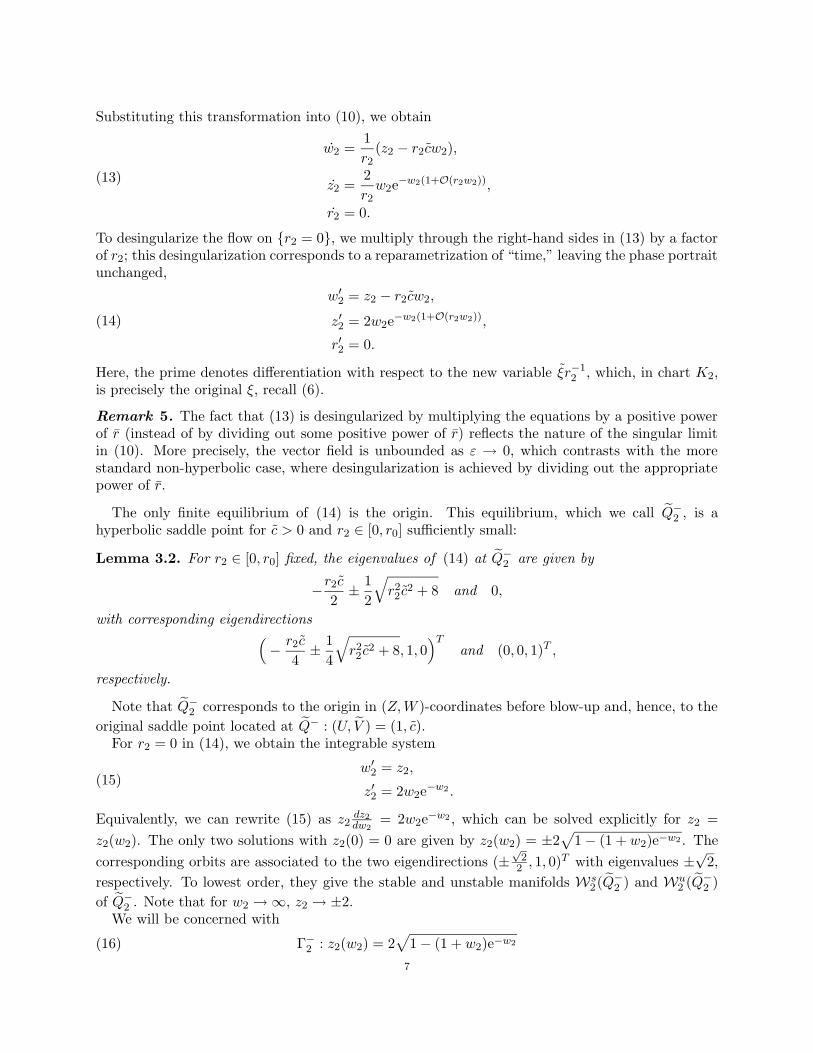
Substituting this transformation into (10), we obtain

w2 =1

r2(z2 − r2cw2),

z2 =2

r2w2e

−w2(1+O(r2w2)),

r2 = 0.

(13)

To desingularize the flow on r2 = 0, we multiply through the right-hand sides in (13) by a factorof r2; this desingularization corresponds to a reparametrization of “time,” leaving the phase portraitunchanged,

w′2 = z2 − r2cw2,

z′2 = 2w2e−w2(1+O(r2w2)),

r′2 = 0.

(14)

Here, the prime denotes differentiation with respect to the new variable ξr−12 , which, in chart K2,

is precisely the original ξ, recall (6).

Remark 5. The fact that (13) is desingularized by multiplying the equations by a positive powerof r (instead of by dividing out some positive power of r) reflects the nature of the singular limitin (10). More precisely, the vector field is unbounded as ε → 0, which contrasts with the morestandard non-hyperbolic case, where desingularization is achieved by dividing out the appropriatepower of r.

The only finite equilibrium of (14) is the origin. This equilibrium, which we call Q−2 , is a

hyperbolic saddle point for c > 0 and r2 ∈ [0, r0] sufficiently small:

Lemma 3.2. For r2 ∈ [0, r0] fixed, the eigenvalues of (14) at Q−2 are given by

−r2c2

± 1

2

√r22 c

2 + 8 and 0,

with corresponding eigendirections(− r2c

4± 1

4

√r22 c

2 + 8, 1, 0)T

and (0, 0, 1)T ,

respectively.

Note that Q−2 corresponds to the origin in (Z,W )-coordinates before blow-up and, hence, to the

original saddle point located at Q− : (U, V ) = (1, c).For r2 = 0 in (14), we obtain the integrable system

w′2 = z2,

z′2 = 2w2e−w2 .

(15)

Equivalently, we can rewrite (15) as z2dz2

dw2= 2w2e

−w2 , which can be solved explicitly for z2 =

z2(w2). The only two solutions with z2(0) = 0 are given by z2(w2) = ±2√

1 − (1 + w2)e−w2 . The

corresponding orbits are associated to the two eigendirections (±√

22 , 1, 0)

T with eigenvalues ±√

2,

respectively. To lowest order, they give the stable and unstable manifolds W s2(Q−

2 ) and Wu2 (Q−

2 )

of Q−2 . Note that for w2 → ∞, z2 → ±2.

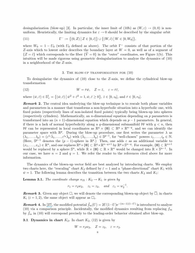
We will be concerned with

Γ−2 : z2(w2) = 2

√1 − (1 + w2)e−w2(16)

7

2

Γ−

2

Σout

2

Q−

2

z2

w2

r2

(a) The “rescaling” chart K2.

P1

`1

Γ+

1

Γ−

1

Σout1

Σin1

ε1

r1

z1

(b) The “phase-directional” chart K1.

Figure 2. The dynamics in the two charts.

here, since it corresponds to the singular orbit Γ− before blow-up. See Figure 2(a) for a summaryof the geometry in chart K2.

Remark 6. Equations (15) correspond precisely to the leading-order “inner system” obtained in[27] by means of asymptotic analysis.

3.2. Dynamics in chart K1. In chart K1, we have

W = r1, Z = z1, ε = r1ε1

for the blow-up transformation in (12), which implies

r′1 = r1(z1 − r1c),

z′1 =2

ε21e− 1

ε1(1+O(r1))

,

ε′1 = −ε1(z1 − r1c)

(17)

for the equations in (10) after desingularization, i.e., after multiplication by r1.Since we assume that r1 is small, the equilibria of (17) are located on the line `1 =

(0, z1, 0)

∣∣ z1 ∈[0, z0]

. Note that although the vector field in (17) is, at first sight, not defined for ε1 = 0, it extends

for ε1 → 0 to a C∞ vector field, since O(r1) stands for an analytic function which is strictly positive;in fact, all of the coefficients in O(r1) are positive, see (9). Therefore, given the above analysis ofthe dynamics in K2, it follows with z1 = z2 that we can restrict ourselves to |z1 − 2| ≤ α here, withα > 0 small. We will denote the point (0, 2, 0) ∈ `1 by P1 in the following.

Lemma 3.3. The eigenvalues of (17) at P1 ∈ `1 are given by −2, 0, and 2, with correspondingeigendirections (0, 0, 1)T , (0, 1, 0)T , and (1, 0, 0)T , respectively.

8

Q−

P

2

Γ+

Γ−

Wu

(Q−

)

ε

w

z

r1

z1

ε1

r2

z2

w2

Figure 3. The situation in blown-up coordinates. (Here, the coordinate framesfor charts K1 and K2 only serve to recall the relevant variables, and not to set therespective origins.)

Given (16) and Lemma 3.1, we obtain an explicit expression for the singular orbit Γ−1 on the

blown-up locus r1 = 0 in chart K1 via

Γ−1 : z1(ε1) = 2

√1 − (1 + 1

ε1)e

− 1

ε1 ;

in particular, z1 → 2 as ε1 → 0, where z1(ε1) is an infinitely flat function at ε1 = 0 (i.e., at P1).The geometry in chart K1 is summarized in Figure 2(b), while the global, blown-up situation is

illustrated in Figure 3.

3.3. Regularity of the transition in K1. For the proof of Theorem 1.1, we will require asmoothness result on the transition past `1 under the flow of (17). For convenience, we introducetwo sections Σin

1 and Σout1 , with ε1 = δ in Σin

1 and r1 = ρ in Σout1 for δ, ρ sufficiently small and

positive. Note that both δ and ρ are constant, i.e., independent of ε. More precisely, we define

Σin1 =

(εδ−1, zin

1 , δ)∣∣ |zin

1 − 2| ≤ α

and Σout1 =

(ρ, zout

1 , ερ−1)∣∣ |zout

1 − 2| ≤ α,(18)

with α > 0 a small constant, as before, and write Π1 : Σin1 → Σout

1 for the corresponding transitionmap, see again Figure 2(b).

Proposition 3.4. The map

Π1 :

Σin

1 → Σout1 ,

(εδ−1, zin1 , δ) 7→ (ρ, zout

1 , ερ−1)

is C∞-smooth in zin1 , as well as in the parameters ε and c.

9

Proof. For convenience, we simplify the equations in (17) by dividing out a factor of (z1−r1c) fromthe right-hand sides,

r′1 = r1,(19a)

z′1 =2

ε21(z1 − r1c)e− 1

ε1(1+O(r1))

,(19b)

ε′1 = −ε1.(19c)

Here, the prime now denotes differentiation with respect to a rescaled variable ξ1. The equationsfor r1 and ε1 are readily solved, since it follows from (19a) and (19c) as well as from rin

1 = εδ−1

and εin1 = δ that

r1 =ε

δeξ1 and ε1 = δe−ξ1 .(20)

In particular, the transition “time” from Σin1 to Σout

1 under Π1 can be obtained explicitly as Ξ1 =− ln ε

δρ, since εout

1 = ερ−1.

It only remains to investigate the regularity of zout1 = zout

1 (zin1 , ε, c). To that end, we introduce

the new variable z1 via z1 = 2 + z1 and then expand (2 + z1 − r1c)−1 = 1

2(1 + O(z1, r1c)) in (19b)to obtain

z′1 =1

ε21e− 1

ε1(1+O(r1))(

1 + O(z1, r1c)).

We now define x1 = δ−1eξ1 and Z1(x1) = z1(ξ1). Note that x1 ∈ [δ−1, ρε−1] and hence εx1 ∈[εδ−1, ρ] ⊂ [0, ρ]; in particular, it follows that εx1 is bounded. We obtain

dZ1

dx1= x1e

−x1(1+O(εx1))(1 + O(Z1, εx1c)

),

or, equivalently,

dZ1

dξ1= 1 + O(Z1, εx1c),(21a)

dx1

dξ1=

1

x1ex1(1+O(εx1))(21b)

for some ξ1. Now, it is important to note that

x1e−x1(1+O(εx1)) ∈

[ρεe−

ρε(1+O(ρ)), 1

δe−

1

δ(1+O( ε

δ))]⊂

[0, 1

δe−

1

δ

];

here, we have used the fact that O(εx1) in (21b) stands for an analytic function which is strictlypositive, see (9). We can solve (21b) by separation of variables,

dξ1 = x1e−x1(1+O(εx1))dx1 = dΨ(x1, εx1),

which gives

ξ1(x1) = Ψ(x1, εx1) − Ψ(δ−1, εδ−1)

if we impose ξ1(δ−1) = 0. Here, Ψ is C∞-smooth due to the analyticity of the vector field in (21)

for x1 > 0. Moreover, Ψ is bounded, since

0 <dξ1

dx1< x1e

−x1 .

Therefore, we conclude that we can solve for x1 = x1(ξ1) in a unique manner, with x1 C∞-smooth.

In turn, since εx1 is bounded, there exists a unique solution Z1 = Z1(Zin1 , ξ1(x1), c) to (21a)

which is C∞-smooth in all its arguments as long as we restrict ourselves to ξ1 ∈ [0, ξout1 ], where

10

ξout1 = ξ1(ρε

−1) = Ψ(ρε−1, ρ) − Ψ(δ−1, εδ−1). Reverting to the original variables z1 and ξ, we findthat zout

1 = zout1 (zin

1 , ε, c) is C∞-smooth in zin1 , as well as in ε and c. This completes the proof.

Remark 7. We conjecture that Π1 is “infinitely close” to the identity, since the right-hand sidein (19b), as well as all its derivatives, go to zero as ε→ 0. A proof would, however, be outside thescope of this work.

Remark 8. Lemma 3.3 shows that the equilibrium at P1 is resonant, in the sense that the eigen-values of the corresponding linearization are in resonance. This implies that resonant terms ofthe form rk

1z`1ε

k1 (k, ` ∈ N) will potentially occur in the normal form for (19b), which, in turn,

might induce logarithmic (switchback) terms [13, 23, 26, 20] in the expansion of Π1. However,Proposition 3.4 implies that no such terms will arise in our case, as Π1 is regular in ε.

4. Proof of Theorem 1.1

The proof of our main result, Theorem 1.1, will be split up into the proofs of several subresults;indeed, Lemma 4.1, Proposition 4.2, and Lemma 4.3 below together immediately yield Theorem 1.1.First, we derive the leading-order behavior of c:

Lemma 4.1. There holds c = 2 + O(1).

Proof. Recall that the analysis in chart K2 implies z2 → 2 as w2 → ∞ to lowest order on Wu(Q−2 ),

see the expression for Γ−2 in (16). Since w2 → ∞ is equivalent to ε1 → 0, cf. Lemma 3.1, and since

z2 = z1, it follows that (r1, z1, ε1) → (0, 2, 0) = P1 ∈ `1. Recalling the definition of Z = −(V − c), as

well as that Z = z1, we have V − c→ −2. Since Ws(Q+) is to leading order given by Γ+ : V = 0,we have c ∼ 2, which is the desired result.

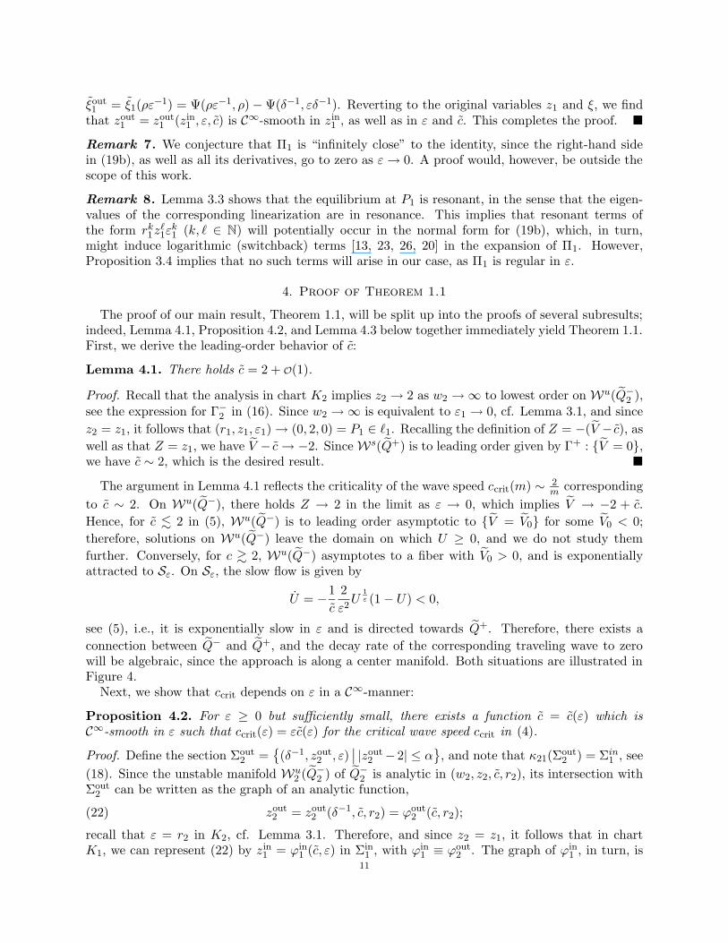
The argument in Lemma 4.1 reflects the criticality of the wave speed ccrit(m) ∼ 2m

corresponding

to c ∼ 2. On Wu(Q−), there holds Z → 2 in the limit as ε → 0, which implies V → −2 + c.

Hence, for c . 2 in (5), Wu(Q−) is to leading order asymptotic to V = V0 for some V0 < 0;

therefore, solutions on Wu(Q−) leave the domain on which U ≥ 0, and we do not study them

further. Conversely, for c & 2, Wu(Q−) asymptotes to a fiber with V0 > 0, and is exponentiallyattracted to Sε. On Sε, the slow flow is given by

U = −1

c

2

ε2U

1

ε (1 − U) < 0,

see (5), i.e., it is exponentially slow in ε and is directed towards Q+. Therefore, there exists a

connection between Q− and Q+, and the decay rate of the corresponding traveling wave to zerowill be algebraic, since the approach is along a center manifold. Both situations are illustrated inFigure 4.

Next, we show that ccrit depends on ε in a C∞-manner:

Proposition 4.2. For ε ≥ 0 but sufficiently small, there exists a function c = c(ε) which isC∞-smooth in ε such that ccrit(ε) = εc(ε) for the critical wave speed ccrit in (4).

Proof. Define the section Σout2 =

(δ−1, zout

2 , ε)∣∣ |zout

2 − 2| ≤ α, and note that κ21(Σ

out2 ) = Σin

1 , see

(18). Since the unstable manifold Wu2 (Q−

2 ) of Q−2 is analytic in (w2, z2, c, r2), its intersection with

Σout2 can be written as the graph of an analytic function,

zout2 = zout

2 (δ−1, c, r2) = ϕout2 (c, r2);(22)

recall that ε = r2 in K2, cf. Lemma 3.1. Therefore, and since z2 = z1, it follows that in chartK1, we can represent (22) by zin

1 = ϕin1 (c, ε) in Σin

1 , with ϕin1 ≡ ϕout

2 . The graph of ϕin1 , in turn, is

11

Q+

Q−

S0

Γ+

Γ−

U0 1

V

U

(a) The geometry for c . 2.

U0 1

Q−

Q+

S0

Γ+

Γ−

U

V

(b) The geometry for c & 2.

Figure 4. The criticality of c ∼ 2.

mapped, under the C∞ mapping Π1, to the graph of a C∞-smooth function in Σout1 ,

zout1 = zout

1 (ρ, c, ερ−1) = ϕout1 (c, ε),(23)

see Proposition 3.4. Hence, in sum, (23) represents the intersection of κ21(Wu2 (Q−

2 )) with Σout1 .

Moreover, since (14) does not depend on c when r2(= ε) = 0, it follows that ∂∂cϕout

1 (2, 0) = 0.

Next, in Σout1 , we can also represent the intersection of Ws(Q+) as the graph of a C∞-smooth

function,

zout1 = ψout

1 (c, ε).

Furthermore, it follows from (5) that ∂∂cψout

1 (2, 0) = 1.Finally, combining the two results from above, we see that the function c(ε) is determined by

the implicit equation

D(c, ε) := ϕout1 (c, ε) − ψout

1 (c, ε) = 0.

In addition, the above analysis shows that

D(2, 0) = 0 and∂D∂c

(2, 0) = −1 6= 0.

Therefore, the result follows locally near (c, ε) = (2, 0) by the Implicit Function Theorem.

Finally, we compute the second-order coefficient in the expansion for ccrit.

Lemma 4.3. There holds c(ε) = 2 + σε+ O(ε2), where

σ = limω0→∞

∫ ω0

0

[ω2e−ω

√1 − (1 + ω)e−ω

− ω3

2e−ω

]dω ≈ −0.3119.

12

Proof. The unstable manifold Wu2 (Q−

2 ) of Q−2 is analytic in w2, z2, c, and r2. Hence, it follows from

regular perturbation theory that, on any bounded domain, we can make the ansatz

z2(w2, c, r2) =∞∑

j=0

Z2j(w2, c)r

j2 and c(r2) =

∞∑

j=0

Cjrj2,(24)

with Z2j(0, c) = 0 for j ≥ 0, in K2. We will consider w2 ∈ [0, δ−1] in the following; recall

the definition of Σout2 . Substituting (24) into (14), making use of the Chain Rule, expanding

exp[− w2

(r2w2

2 +r2

2w2

2

3 + . . .)]

, and collecting like powers of r2, we obtain a recursive sequence ofdifferential equations for Z2j

which depend on Cj (j ≥ 0):

O(1) :dZ20

dw2Z20

= 2w2e−w2 ,(25)

O(r2) :d

dw2(Z20

Z21) = C0w2

dZ20

dw2− w3

2e−w2 .(26)

Equation (25) is equivalent to (15); hence, Z20equals z2 as defined in (16). Next, we can solve (26)

using integration by parts,

Z21(w2, c) =

1√1 − (1 + w2)e−w2

∫ w2

0

[ω2e−ω

√1 − (1 + ω)e−ω

− ω3

2e−ω

]dω

= 2w2 −1√

1 − (1 + w2)e−w2

∫ w2

0

[2√

1 − (1 + ω)e−ω + ω3e−ω]dω,

(27)

where the constant of integration is chosen such that Z21(0, c) = 0 and we have used C0 = 2. In

particular, in Σout2 , the expansion for Wu

2 (Q−2 ) is given by

zout2 = z2(δ

−1) ∼ Z20(δ−1) + εZ21

(δ−1, C0).(28)

We now need to investigate the asymptotics of Wu2 (Q−

2 ) as w2 → ∞. This is readily done in K1,i.e., we will study the transition from Σin

1 = κ21(Σout2 ) to Σout

1 .Let Π1 be defined as in Proposition 3.4, and assume that a curve of initial conditions for Π1

is given by (εδ−1, zin1 , δ) ∈ Σin

1 , with zin1 = zout

2 as in (28). Since Π1 is C∞-smooth in ε, seeProposition 3.4, we may expand z1 as

z1(ε1, c, ε) ∼ Z10(ε1, c) + εZ11

(ε1, c).

Substituting this expansion, as well as the expansion for c from (24), into the equations in (17) andcomparing powers of ε, we obtain the equations

O(1) :dZ10

dε1Z10

= − 2

ε31e− 1

ε1 ,(29)

O(ε) :d

dε1(Z10

Z11) =

2

ε1

dZ10

dε1+

e− 1

ε1

ε51,(30)

which correspond precisely to (25) and (26) after transformation to K1. One can check that thecorresponding solutions Z10

and Z11are given by κ21(Z20

) and κ21(Z21), respectively. In particular,

given (28) as well as εout1 = ερ−1, we find that zout

1 = Π1(zin1 ) is obtained as

zout1 ∼ 2

√1 − (1 + ρ

ε)e−

ρε +

ε√1 − (1 + ρ

ε)e−

ρε

∫ ∞

ερ

[e− 1

η

η4

√1 − (1 + 1

η)e

− 1

η

− 1

2

e− 1

η

η5

]dη

︸ ︷︷ ︸=:I( ε

ρ)

.(31)

13

To determine C1, we have to match Wu(Q−) to Ws(Q+) in the overlap domain between theinner and outer regions. Without loss of generality, the matching will be done in Σout

1 . Recalling

that V = 0 to all orders in ε on Ws(Q+), we conclude Z = c and hence zout1 ∼ 2 + εC1 in Σout

1 forthe contribution from the outer problem. To leading order, we retrieve c = 2 (up to exponentiallysmall terms in ε). To match the O(ε)-terms in (31) to εC1, note that

I( ερ) = I(0) + O(e−

κε ) for some κ > 0,

since the corresponding integrand is exponentially small on [0, ερ] and since ρ > 0. Evaluating I(0)

numerically, we find C1 ∼ I(0) ≈ −0.3119. This completes the proof.

The numerical value of σ coincides with the result obtained in [19] by means of asymptoticmatching. In fact, the above analysis is closely related to the approach one would take to determinean expansion for ccrit via the method of matched asymptotics: The “inner expansion” coming fromchart K2 is “matched” to the “outer expansion” derived in chart K1 in the overlap domain betweenthe two charts. Note that this overlap domain corresponds to the classical “intermediate region”where one would typically match by defining an “intermediate variable”.

Remark 9. Given the regularity of Π1, it is not surprising that the analysis in K1 is analogous tothat in K2, and that the resulting expansions are equal up to the coordinate change κ21. Althoughfor ε > 0, one could probably restrict oneself toK2, it seems more natural to analyze the asymptoticsfor w2 → ∞ in K1.

Remark 10. Numerical evidence [27] suggests that the one-term truncation of the asymptoticexpansion for ccrit in (2), ccrit(m) ∼ 2

m, is optimal for m ∈ [2,m1), where m1 ≈ 4. Similarly,

it appears that the two-term truncation is optimal on some finite m-interval (m1,m2), with m1

defined as before. This would indicate that the formal expansion for ccrit(m) might well haveGevrey properties, cf. e.g. [24]. A rigorous analysis of this question, including the calculationof the corresponding optimal truncation points, seems to be an interesting problem for furtherstudy. The geometric desingularization presented in this article might well be useful for such ananalysis. See e.g. [16] for an example of how the blow-up technique can be employed to studyGevrey properties.

Acknowledgment. The authors are grateful to Tom Witelski for comments on the original manu-script. F.D. would like to thank the Department of Mathematics and Statistics at Boston Universityfor its hospitality and support during the preparation of this paper. The research of N.P. and T.J.K.was supported in part by NSF grants DMS-0109427 and DMS-0306523, respectively.

References

[1] J. Billingham. Phase plane analysis of one-dimensional reaction-diffusion waves with degenerate reaction terms.Dyn. Stab. Syst., 15(1):23–33, 2000.

[2] N.F. Britton. Reaction-Diffusion Equations and Their Applications to Biology. Academic Press Inc., London,1986.

[3] F. Dumortier. Techniques in the theory of local bifurcations: blow-up, normal forms, nilpotent bifurcations,singular perturbations. In D. Schlomiuk, editor, Bifurcations and Periodic Orbits of Vector Fields, volume 408of NATO Adv. Sci. Inst. Ser. C Math. Phys. Sci., pages 19–73, Dordrecht, 1993. Kluwer Acad. Publ.

[4] F. Dumortier and P. De Maesschalck. Topics in singularities and bifurcations of vector fields. In Y. Ilyashenko,C. Rousseau, and G. Sabidussi, editors, Normal Forms, Bifurcations, and Finiteness Problems in DifferentialEquations, volume 137 of NATO Sci. Ser. II Math. Phys. Chem., pages 33–86, Dordrecht, 2004. Kluwer Acad.Publ.

[5] F. Dumortier and R. Roussarie. Canard cycles and center manifolds. Mem. Amer. Math. Soc., 121(577), 1996.[6] F. Dumortier and R. Roussarie. Geometric singular perturbation theory beyond normal hyperbolicity. In

C.K.R.T. Jones and A. Khibnik, editors, Multiple-time-scale dynamical systems, volume 122 of IMA Vol. Math.Appl., pages 29–63, New York, 2001. Springer-Verlag.

14

[7] F. Dumortier, R. Roussarie, and J. Sotomayor. Bifurcations of cuspidal loops. Nonlinearity, 10(6):1369–1408,1997.

[8] N. Fenichel. Persistence and smoothness of invariant manifolds for flows. Indiana Univ. Math. J., 21:193–226,1971.

[9] N. Fenichel. Geometric singular perturbation theory for ordinary differential equations. J. Differential Equations,31(1):53–98, 1979.

[10] R.A. Fisher. The wave of advance of advantageous genes. Ann. Eugenics, 7:355–369, 1937.[11] C.K.R.T. Jones. Geometric Singular Perturbation Theory. In Dynamical Systems, volume 1609 of Springer

Lecture Notes in Mathematics, New York, 1995. Springer-Verlag.[12] A.N. Kolmogorov, I.G. Petrowskii, and N. Piscounov. Etude de l’equation de la diffusion avec croissance de la

quantite de matiere et son application a un probleme biologique. Moscow Univ. Math. Bull., 1:1–25, 1937.[13] M. Krupa and P. Szmolyan. Extending geometric singular perturbation theory to nonhyperbolic points–fold and

canard points in two dimensions. SIAM J. Math. Anal., 33(2):286–314, 2001.[14] M. Krupa and P. Szmolyan. Relaxation oscillation and canard explosion. J. Differential Equations, 174(2):312–

368, 2001.[15] J.A. Leach, D.J. Needham, and A.L. Kay. The evolution of reaction-diffusion waves in a class of reaction-diffusion

equations: algebraic decay rates. Phys. D, 167(3-4):153–182, 2002.[16] P. De Maesschalck. Gevrey properties of real, planar singularly perturbed systems. Preprint, 2005.[17] J.H. Merkin and D.J. Needham. Reaction-diffusion waves in an isothermal chemical system with general orders

of autocatalysis and spatial dimension. J. Appl. Math. Phys. (ZAMP) A, 44(4):707–721, 1993.[18] D.J. Needham and A.N. Barnes. Reaction-diffusion and phase waves occurring in a class of scalar reaction-

diffusion equations. Nonlinearity, 12(1):41–58, 1999.[19] K. Ono. Analytical methods for reaction-diffusion equations: critical wave speeds and axi-symmetric phenomena.

PhD thesis, Boston University, Boston, MA, U.S.A., 2001.[20] N. Popovic. A geometric analysis of logarithmic switchback phenomena. In M.P. Mortell, R.E. O’Malley Jr.,

A.V. Pokrovskii, and V.A. Sobolev, editors, International Workshop on Hysteresis & Multi-scale Asymptotics,University College Cork, Ireland, 17-21 March 2004, volume 22 of J. Phys. Conference Series, pages 164–173,Bristol and Philadelphia, 2005. Inst. Phys. Publishing.

[21] N. Popovic and T.J. Kaper. Rigorous asymptotic expansions for critical wave speeds in a family of scalar reaction-diffusion equations. J. Dynam. Differential Equations, 2006. To appear.

[22] N. Popovic and P. Szmolyan. A geometric analysis of the Lagerstrom model problem. J. Differential Equations,199(2):290–325, 2004.

[23] N. Popovic and P. Szmolyan. Rigorous asymptotic expansions for Lagerstrom’s model equation–a geometricapproach. Nonlinear Anal., 59(4):531–565, 2004.

[24] J.P. Ramis. Series divergentes et theories asymptotiques. Bull. Soc. Math. France, 121, 1993.[25] J.A. Sherratt and B.P. Marchant. Algebraic decay and variable speeds in wavefront solutions of a scalar reaction-

diffusion equation. IMA J. Appl. Math., 56(3):289–302, 1996.[26] S. van Gils, M. Krupa, and P. Szmolyan. Asymptotic expansions using blow-up. Z. Angew. Math. Phys. (ZAMP),

56(3):369–397, 2005.[27] T.P. Witelski, K. Ono, and T.J. Kaper. Critical wave speeds for a family of scalar reaction-diffusion equations.

Appl. Math. Lett., 14(1):65–73, 2001.

E-mail address: freddy.dumortier@uhasselt.be, popovic@math.bu.edu, tasso@math.bu.edu

Universiteit Hasselt, Campus Diepenbeek, Agoralaan Gebouw D, B-3590 Diepenbeek, Belgium

Boston University, Center for BioDynamics and Department of Mathematics and Statistics, 111

Cummington Street, Boston, MA 02215, U.S.A.

15