water

Article

Non-Stationary Bayesian Modeling of AnnualMaximum Floods in a Changing Environmentand Implications for Flood Management in theKabul River Basin, Pakistan

Asif Mehmood 1,2, Shaofeng Jia 1,2,* , Rashid Mahmood 1,2 , Jiabao Yan 1,2 and Moien Ahsan 3

1 Key Laboratory of Water Cycle and Related Land Surface Processes/Institute of Geographic Sciences andNatural Resources Research (IGSNRR), Chinese Academy of Sciences (CAS), Beijing 100101, China;engrasifmehmood733@gmail.com (A.M.); rashi1254@gmail.com (R.M.); jiabao.yan@foxmail.com (J.Y.)

2 University of Chinese Academy of Sciences, Beijing 100049, China3 Center of Excellence in Water Resources Engineering (CEWRE), UET, Lahore 54890, Pakistan;

Moien_ag_2232@yahoo.com* Correspondence: jiasf@igsnrr.ac.cn; Tel.: +86-10-6485-6539

Received: 20 May 2019; Accepted: 3 June 2019; Published: 14 June 2019�����������������

Abstract: Recent evidence of regional climate change associated with the intensification of humanactivities has led hydrologists to study a flood regime in a non-stationarity context. This studyutilized a Bayesian framework with informed priors on shape parameter for a generalized extremevalue (GEV) model for the estimation of design flood quantiles for “at site analysis” in a changingenvironment, and discussed its implications for flood management in the Kabul River basin (KRB),Pakistan. Initially, 29 study sites in the KRB were used to evaluate the annual maximum flood regimeby applying the Mann–Kendall test. Stationary (without trend) and a non-stationary (with trend)Bayesian models for flood frequency estimation were used, and their results were compared usingthe corresponding flood frequency curves (FFCs), along with their uncertainty bounds. The resultsof trend analysis revealed significant positive trends for 27.6% of the gauges, and 10% showedsignificant negative trends at the significance level of 0.05. In addition to these, 6.9% of the gaugesalso represented significant positive trends at the significance level of 0.1, while the remaining stationsdisplayed insignificant trends. The non-stationary Bayesian model was found to be reliable for studysites possessing a statistically significant trend at the significance level of 0.05, while the stationaryBayesian model overestimated or underestimated the flood hazard for these sites. Therefore, it isvital to consider the presence of non-stationarity for sustainable flood management under a changingenvironment in the KRB, which has a rich history of flooding. Furthermore, this study also statesa regional shape parameter value of 0.26 for the KRB, which can be further used as an informedprior on shape parameter if the study site under consideration possesses the flood type “flash”.The synchronized appearance of a significant increase and decrease of trends within very closegauge stations is worth paying attention to. The present study, which considers non-stationarityin the flood regime, will provide a reference for hydrologists, water resource managers, planners,and decision makers.

Keywords: non-stationary; extreme value theory; uncertainty; flood regime; flood management;Kabul river basin; Pakistan

1. Introduction

The comprehensive understanding of flood regimes is an important challenge in hydrology.Hydrologists and engineers customarily use flood frequency analysis (FFA) as a tool to understand

Water 2019, 11, 1246; doi:10.3390/w11061246 www.mdpi.com/journal/water

Water 2019, 11, 1246 2 of 30

flood regimes throughout the world. FFA estimates the flood peak for a given return period, but thecurrently used methods of FFA assume that the flood time series are independent and identicallydistributed [1–3] or, in other words, have no trends and unanticipated variations [4]. Indeed, the conceptof stationarity was and is being adopted to design water resources infrastructure and flood protectionworks all around the globe. In recent decades, the climate system has been under stress due to naturalvariations in the global climate, and human activity also has a potential influence on regional climatethat is ultimately intensifying the hydrologic cycle [5]. The hypothesis of stationarity has becomewidely questionable due to this regional and global change. Keeping this point of view, several studieshave tried to explore the validity of this hypothesis in flood regimes in many regions around the world,considering the effect of natural climate variability [6–12] or land use changes [13–15]. The results ofthese studies have shown clear violations of the assumption of stationarity, which is consistent withstudies that indicate an intensification of the hydrologic cycle [16,17].

Particularly, the KRB in the Hindu Kush Himalayan Range (HKH) is exposed to disturbancesfrom the South Asian monsoon originating from the Bay of Bengal. Several recent studies representeda paucity of stationarity and indicated the intensification in some elements of the hydrologic cycleat the regional scale. The results of these studies investigated the change in the rainfall regime ofthe KRB. For instance, the number of consecutive wet days has been increasing significantly in thePeshawar valley, with a total change of 2.16 at a 95% confidence level. Consecutive wet days havealso increased at Saidu Sharif in the Swat valley and Chitral [18]. Ahmad et al. [19] investigatedtrends in rainfall over the entire Swat River basin, a sub-basin of the KRB. They observed the highestpositive trend (7.48 mm year−1) at the Saidu Sharif in Swat valley. For annual precipitation time series,statistically insignificant trends were revealed for the whole Swat River basin. However, significantpositive increasing trends of precipitation (2.18 mm year−1) were observed in the Lower Swat basin.Saidu Sharif, Mardan, and Charsada stations showed significant positive trends (increased precipitationover time) at the 5% significance level in the annual precipitation time series [20]. The results of thesestudies revealed the presence of trends in precipitation, and their conclusions suggest an importantlink between the changes exhibited in hydro-climatic variables [21].

Furthermore, other factors that may affect the magnitude and frequency of floods in the KRBare associated with human-induced alterations, such as changes in land use, deforestation, and damconstruction. In the KRB, the human activities that can considerably influence flood frequency areland use changes linked with population increase. For instance, a recent study regarding land usecover change (LUCC) dynamics in the KRB in Afghanistan highlighted that substantial LUCCs haveoccurred during the time interval 2000–2010; among several land cover classes, forest, cultivatedland, and grassland showed dynamical change. During the study period, one-fourth of the forestarea was lost, while cultivated land and grassland showed an increase of 13% and 11%, respectively.The forest area was mainly transformed into grassland and barren land. Unused land was changedinto built-up areas, up to 2%, and water areas increased by 4%. A total loss of 43% was observed inforest area [22]. Similarly, LUCCs in the Swat valley have also occurred. Deforestation occurring dueto agriculture expansion was 11.4% at a rate of 0.29%, 77.6% at a rate of 1.98%, and 129.9% at a rate of3.3%, annually in Kalam, Malam Jaba, and the Swat district areas, respectively. The rangeland hasincreased due to the conversion of forest land from 1968–1990, by about 158.7%, 38.18%, and 22.2%in Kalam, Malam Jaba, and Swat regions, respectively, while a 13.22% increase has occurred from1990 to 2007 due to the conversion of agriculture land to rangeland [23]. Dir Kohistan areas of theHindu Kush Mountains, the northern regions of Pakistan, also showed a 6.4% decrease in forestcover, 22.1% increase in rangeland, and 2.9% increase in agriculture land [24,25]. Similarly, Ahmadand Nizami [26] reported a 7.64% decrease in total area under rangeland in Kumrat valley, HinduKush regions. The Mardan city–Kalpani River basin showed an increase in built-up area by 30–60%during 1990–2010. An increase in built-up area has doubled the impervious surface in Mardan andthe agriculture land has shrunk from 42% to 35% [27]. Similar results were presented for Peshawar,the capital city of Khyber Pakhtunkhwa province, Pakistan, indicating a 26.59% increase in built-up

Water 2019, 11, 1246 3 of 30

area during 1999–2016 [28]. The Peshawar valley, with a rich history of flooding, provides the junctionsfor the Kabul River and its various right and left tributaries.

The above studies clearly show the presence of trends in rainfall regime as well as land use changein different sub-basins of the KRB. These climate and human interventions may induce non-stationarityin the flood regime. However, no studies have been reported to examine the presence or absenceof stationarity in the flood regime of the basin. Therefore, it is imperative to study floods with anon-stationary point of view for the KRB.

Recently, Milly et al. [29] stated that the hypothesis of stationarity must be relinquished and that“stationarity is dead” and “should not be revived”. The methods used for estimation of hydrologicindicators should be based on an innovative approach that would be reliable and useful for watermanagement under a changing environment.

In the literature, various approaches have been reported using probabilistic modeling of floodfrequency in a non-stationary context. Khaliq et al. [2] presented a comprehensive review, including theincorporation of trends in the parameters of the distributions, the incorporation of trends in statisticalmoments, the quantile regression method, and the local likelihood method. The studies of FFA undernon-stationary conditions have mostly assumed trends in time [30–37]. The present study outlined aBayesian framework for “at site flood frequency modeling” in stationary and non-stationary conditions.The fundamental concept is based on the generalized extreme value (GEV) distribution, combinedwith Bayesian inference for uncertainty assessment. For this study, a model with trend (non-stationary)and without trend (stationary) was used.

Previous studies in the KRB were limited to inundation mapping of flood-prone areas with a verylittle flow gauge station data, using a traditional frequentist approach [38–42].

The main objectives of the study were: (1) to analyze temporal and spatial trends in the annualmaximum flood regime for the KRB, Pakistan, because no study has yet been reported in the literatureto study the trends in annual extreme data of flood in detail, and (2) to address the non-stationarymodeling of the flood regime in the KRB and its implications for flood management in a changingenvironment. We explored the differences between stationary and non-stationary flood quantileestimates for a given return period using flood frequency curves (FFCs), along with their uncertaintybounds for risk assessment, to analyze the importance of non-stationary models for improving floodmanagement in the study area.

2. Study Area and Data Description

2.1. Study Area

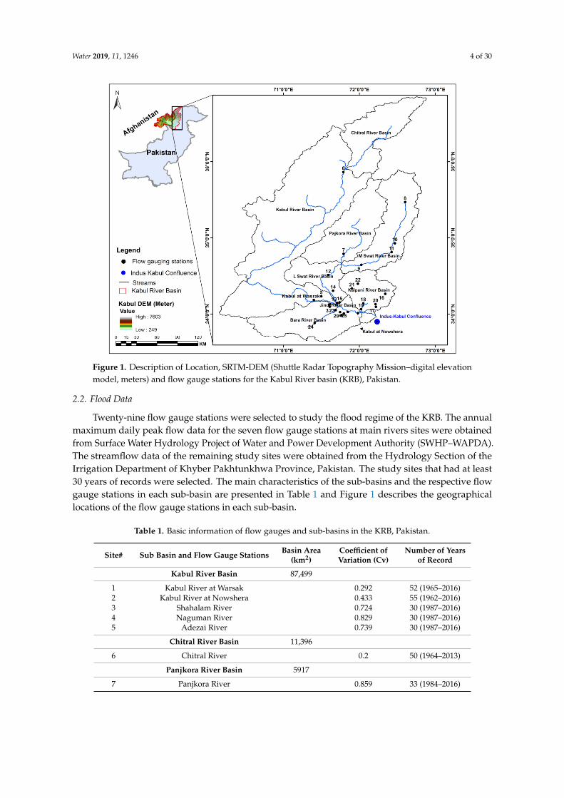
The Kabul River basin (KRB), in Pakistan, stretches from 71◦1′55”–72◦56′0” E to 33◦20′9”–36◦50′0”N, as shown in Figure 1, which covers an area of 33,709 km2. The Kabul River starts at the base ofUnai pass from the Hindu Kush Mountains in Afghanistan and flows eastward, covering a distanceof 700 km to drain into the Indus River, Pakistan [43]. The entire basin covers an area of 87,499 km2.The elevation in the basin varies substantially from 249 m.a.s.l to 7603 m.a.s.l. High elevation mountainsare mainly located in the north. The average temperature and average precipitation vary significantlyacross the River basin. The average temperature is about 13 ◦C. Most of the precipitation occurs in thenorthern mountain and highlands, reported up to 1600 mm. [44].

This study explores the part of the KRB that contributes to flooding. The flood problem arisesmainly as the Kabul River enters Pakistan. The Logar River basin, Alingar River basin, and PanjshirRiver basin lie in Afghanistan. Three dams—Naghlu, Surobi, and Darunta—are located in Afghanistanon the Kabul River and Warsak dam is also located on the Kabul River in Pakistan. The study area isfurther divided into eight sub-basins: Kabul River basin, Chitral River basin, Main Swat River basin,Panjkora River basin, Lower Swat River basin, Kalpani River basin, Jindi River basin, and Bara Riverbasin. The SRTM-DEM (Shuttle Radar Topography Mission–digital elevation model) of 30 m resolutionand the geographical location of the sub-basins are also illustrated in Figure 1.

Water 2019, 11, 1246 4 of 30Water 2019, 11, x FOR PEER REVIEW 4 of 31

Figure 1. Description of Location, SRTM-DEM (Shuttle Radar Topography Mission–digital elevation model, meters) and flow gauge stations for the Kabul River basin (KRB), Pakistan.

2.2. Flood Data

Twenty-nine flow gauge stations were selected to study the flood regime of the KRB. The annual maximum daily peak flow data for the seven flow gauge stations at main rivers sites were obtained from Surface Water Hydrology Project of Water and Power Development Authority (SWHP–WAPDA). The streamflow data of the remaining study sites were obtained from the Hydrology Section of the Irrigation Department of Khyber Pakhtunkhwa Province, Pakistan. The study sites that had at least 30 years of records were selected. The main characteristics of the sub-basins and the respective flow gauge stations in each sub-basin are presented in Table 1 and Figure 1 describes the geographical locations of the flow gauge stations in each sub-basin.

2.3. Flood Generating Mechanism in KRB

The hydrology of floods is linked to weather and climate as well as to physiographical features [45]. The basin has large altitudinal variations from 249 m.a.s.l. to 7603 m.a.s.l. Glacier-melt contribution from the upper part of the basin combined with rainfall in the lower part is the most likely cause of flooding in the region [38]. In the KRB, floods are mostly generated by monsoon rainfall but snow or glacial melt floods have also been observed in some parts of the basin. Snowmelt floods are not common. According to the data used in this study, all of the flood peaks were observed during the monsoon season, from July to August, in almost all the tributaries of the KRB. The historical floods occurred in July 2010, August 1995, and July 1992; all were observed during the monsoon. Anjum et al. [46] provided the details regarding rainfall magnitude, intensity, and spatial extent for the 2010 event. The South Asian monsoon originating from the Bay of Bengal is the dominant weather system for flood generation in the KRB.

However, the flood of 2005 in the Kabul and Indus Rivers was due to snowmelt as well as rainfall in the pre-monsoon period [47]. The flooding behavior of the different tributaries differs according to their catchment characteristics. The riverine floods in the Kabul River usually start below the Warsak dam, and this phenomenon propagates until its confluence with the Indus River at Khairabad

Figure 1. Description of Location, SRTM-DEM (Shuttle Radar Topography Mission–digital elevationmodel, meters) and flow gauge stations for the Kabul River basin (KRB), Pakistan.

2.2. Flood Data

Twenty-nine flow gauge stations were selected to study the flood regime of the KRB. The annualmaximum daily peak flow data for the seven flow gauge stations at main rivers sites were obtainedfrom Surface Water Hydrology Project of Water and Power Development Authority (SWHP–WAPDA).The streamflow data of the remaining study sites were obtained from the Hydrology Section of theIrrigation Department of Khyber Pakhtunkhwa Province, Pakistan. The study sites that had at least30 years of records were selected. The main characteristics of the sub-basins and the respective flowgauge stations in each sub-basin are presented in Table 1 and Figure 1 describes the geographicallocations of the flow gauge stations in each sub-basin.

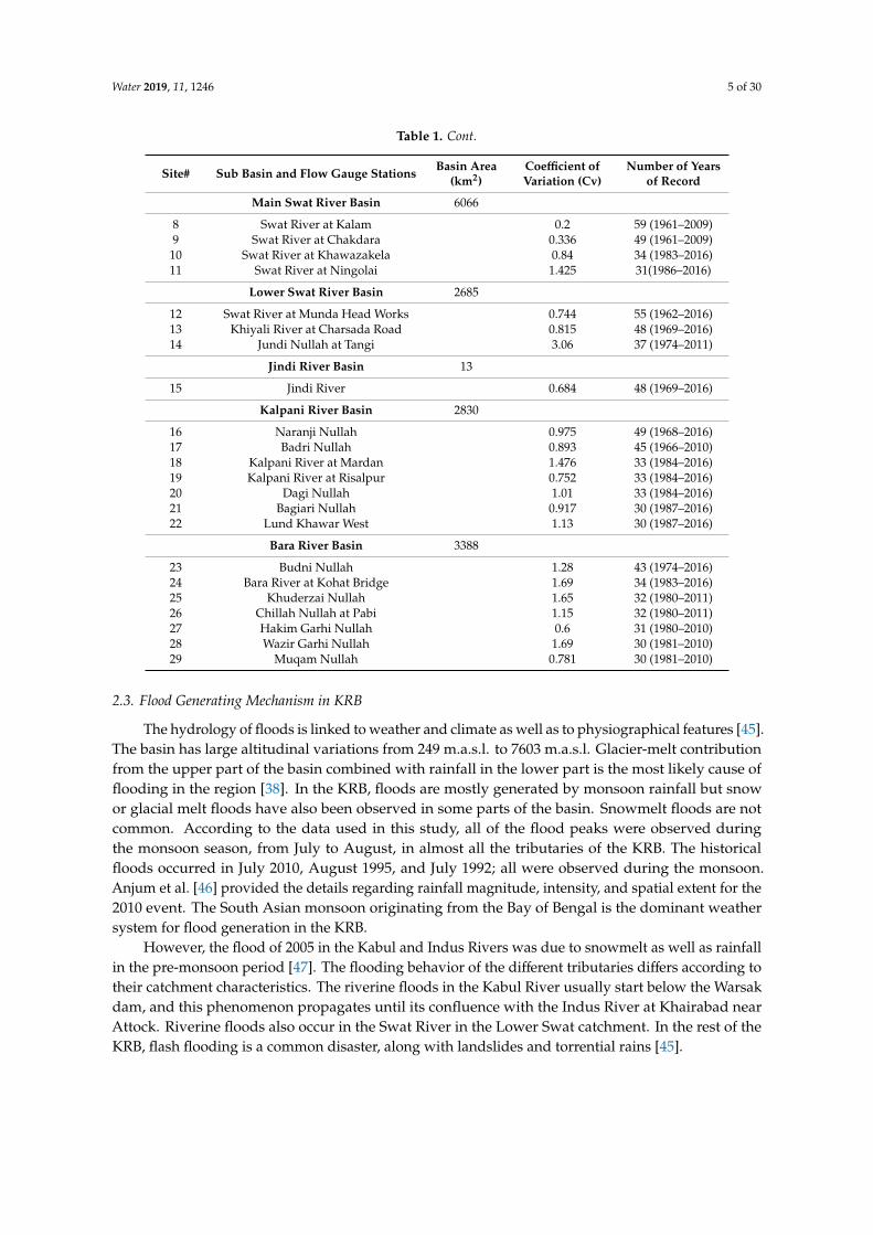
Table 1. Basic information of flow gauges and sub-basins in the KRB, Pakistan.

Site# Sub Basin and Flow Gauge Stations Basin Area(km2)

Coefficient ofVariation (Cv)

Number of Yearsof Record

Kabul River Basin 87,499

1 Kabul River at Warsak 0.292 52 (1965–2016)2 Kabul River at Nowshera 0.433 55 (1962–2016)3 Shahalam River 0.724 30 (1987–2016)4 Naguman River 0.829 30 (1987–2016)5 Adezai River 0.739 30 (1987–2016)

Chitral River Basin 11,396

6 Chitral River 0.2 50 (1964–2013)

Panjkora River Basin 5917

7 Panjkora River 0.859 33 (1984–2016)

Water 2019, 11, 1246 5 of 30

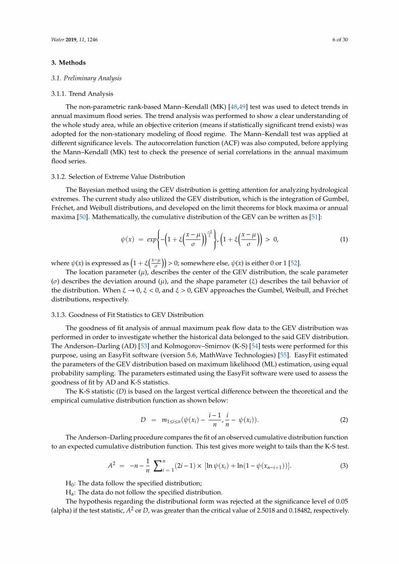
Table 1. Cont.

Site# Sub Basin and Flow Gauge Stations Basin Area(km2)

Coefficient ofVariation (Cv)

Number of Yearsof Record

Main Swat River Basin 6066

8 Swat River at Kalam 0.2 59 (1961–2009)9 Swat River at Chakdara 0.336 49 (1961–2009)10 Swat River at Khawazakela 0.84 34 (1983–2016)11 Swat River at Ningolai 1.425 31(1986–2016)

Lower Swat River Basin 2685

12 Swat River at Munda Head Works 0.744 55 (1962–2016)13 Khiyali River at Charsada Road 0.815 48 (1969–2016)14 Jundi Nullah at Tangi 3.06 37 (1974–2011)

Jindi River Basin 13

15 Jindi River 0.684 48 (1969–2016)

Kalpani River Basin 2830

16 Naranji Nullah 0.975 49 (1968–2016)17 Badri Nullah 0.893 45 (1966–2010)18 Kalpani River at Mardan 1.476 33 (1984–2016)19 Kalpani River at Risalpur 0.752 33 (1984–2016)20 Dagi Nullah 1.01 33 (1984–2016)21 Bagiari Nullah 0.917 30 (1987–2016)22 Lund Khawar West 1.13 30 (1987–2016)

Bara River Basin 3388

23 Budni Nullah 1.28 43 (1974–2016)24 Bara River at Kohat Bridge 1.69 34 (1983–2016)25 Khuderzai Nullah 1.65 32 (1980–2011)26 Chillah Nullah at Pabi 1.15 32 (1980–2011)27 Hakim Garhi Nullah 0.6 31 (1980–2010)28 Wazir Garhi Nullah 1.69 30 (1981–2010)29 Muqam Nullah 0.781 30 (1981–2010)

2.3. Flood Generating Mechanism in KRB

The hydrology of floods is linked to weather and climate as well as to physiographical features [45].The basin has large altitudinal variations from 249 m.a.s.l. to 7603 m.a.s.l. Glacier-melt contributionfrom the upper part of the basin combined with rainfall in the lower part is the most likely cause offlooding in the region [38]. In the KRB, floods are mostly generated by monsoon rainfall but snowor glacial melt floods have also been observed in some parts of the basin. Snowmelt floods are notcommon. According to the data used in this study, all of the flood peaks were observed duringthe monsoon season, from July to August, in almost all the tributaries of the KRB. The historicalfloods occurred in July 2010, August 1995, and July 1992; all were observed during the monsoon.Anjum et al. [46] provided the details regarding rainfall magnitude, intensity, and spatial extent for the2010 event. The South Asian monsoon originating from the Bay of Bengal is the dominant weathersystem for flood generation in the KRB.

However, the flood of 2005 in the Kabul and Indus Rivers was due to snowmelt as well as rainfallin the pre-monsoon period [47]. The flooding behavior of the different tributaries differs according totheir catchment characteristics. The riverine floods in the Kabul River usually start below the Warsakdam, and this phenomenon propagates until its confluence with the Indus River at Khairabad nearAttock. Riverine floods also occur in the Swat River in the Lower Swat catchment. In the rest of theKRB, flash flooding is a common disaster, along with landslides and torrential rains [45].

Water 2019, 11, 1246 6 of 30

3. Methods

3.1. Preliminary Analysis

3.1.1. Trend Analysis

The non-parametric rank-based Mann–Kendall (MK) [48,49] test was used to detect trends inannual maximum flood series. The trend analysis was performed to show a clear understanding ofthe whole study area, while an objective criterion (means if statistically significant trend exists) wasadopted for the non-stationary modeling of flood regime. The Mann–Kendall test was applied atdifferent significance levels. The autocorrelation function (ACF) was also computed, before applyingthe Mann–Kendall (MK) test to check the presence of serial correlations in the annual maximumflood series.

3.1.2. Selection of Extreme Value Distribution

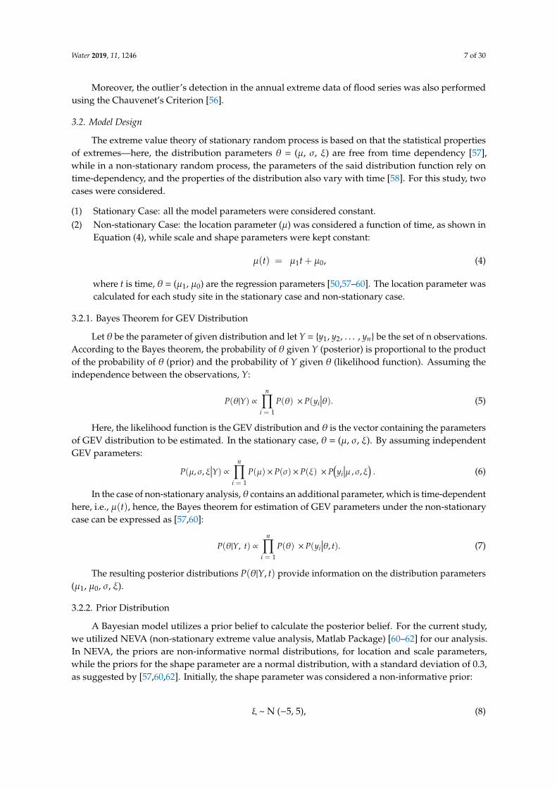
The Bayesian method using the GEV distribution is getting attention for analyzing hydrologicalextremes. The current study also utilized the GEV distribution, which is the integration of Gumbel,Fréchet, and Weibull distributions, and developed on the limit theorems for block maxima or annualmaxima [50]. Mathematically, the cumulative distribution of the GEV can be written as [51]:

ψ(x) = exp

−(1 + ξ(x− µσ

))−1ξ

,(1 + ξ

(x− µσ

))> 0, (1)

where ψ(x) is expressed as(1 + ξ

( x−µσ

))> 0; somewhere else, ψ(x) is either 0 or 1 [52].

The location parameter (µ), describes the center of the GEV distribution, the scale parameter(σ) describes the deviation around (µ), and the shape parameter (ξ) describes the tail behavior ofthe distribution. When ξ→ 0, ξ < 0, and ξ > 0, GEV approaches the Gumbel, Weibull, and Fréchetdistributions, respectively.

3.1.3. Goodness of Fit Statistics to GEV Distribution

The goodness of fit analysis of annual maximum peak flow data to the GEV distribution wasperformed in order to investigate whether the historical data belonged to the said GEV distribution.The Anderson–Darling (AD) [53] and Kolmogorov–Smirnov (K-S) [54] tests were performed for thispurpose, using an EasyFit software (version 5.6, MathWave Technologies) [55]. EasyFit estimatedthe parameters of the GEV distribution based on maximum likelihood (ML) estimation, using equalprobability sampling. The parameters estimated using the EasyFit software were used to assess thegoodness of fit by AD and K-S statistics.

The K-S statistic (D) is based on the largest vertical difference between the theoretical and theempirical cumulative distribution function as shown below:

D = m1≤i≤n(ψ(xi) −i− 1

n,

in− ψ(xi)). (2)

The Anderson–Darling procedure compares the fit of an observed cumulative distribution functionto an expected cumulative distribution function. This test gives more weight to tails than the K-S test.

A2 = −n−1n

∑n

i = 1(2i− 1) × [lnψ(xi) + ln(1−ψ(xn−i+1))]. (3)

H0: The data follow the specified distribution;Ha: The data do not follow the specified distribution.The hypothesis regarding the distributional form was rejected at the significance level of 0.05

(alpha) if the test statistic, A2 or D, was greater than the critical value of 2.5018 and 0.18482, respectively.

Water 2019, 11, 1246 7 of 30

Moreover, the outlier’s detection in the annual extreme data of flood series was also performedusing the Chauvenet’s Criterion [56].

3.2. Model Design

The extreme value theory of stationary random process is based on that the statistical propertiesof extremes—here, the distribution parameters θ = (µ, σ, ξ) are free from time dependency [57],while in a non-stationary random process, the parameters of the said distribution function rely ontime-dependency, and the properties of the distribution also vary with time [58]. For this study, twocases were considered.

(1) Stationary Case: all the model parameters were considered constant.(2) Non-stationary Case: the location parameter (µ) was considered a function of time, as shown in

Equation (4), while scale and shape parameters were kept constant:

µ(t) = µ1t + µ0, (4)

where t is time, θ = (µ1, µ0) are the regression parameters [50,57–60]. The location parameter wascalculated for each study site in the stationary case and non-stationary case.

3.2.1. Bayes Theorem for GEV Distribution

Let θ be the parameter of given distribution and let Y = {y1, y2, . . . , yn} be the set of n observations.According to the Bayes theorem, the probability of θ given Y (posterior) is proportional to the productof the probability of θ (prior) and the probability of Y given θ (likelihood function). Assuming theindependence between the observations, Y:

P(θ|Y) ∝n∏

i = 1

P(θ) × P(yi∣∣∣θ). (5)

Here, the likelihood function is the GEV distribution and θ is the vector containing the parametersof GEV distribution to be estimated. In the stationary case, θ = (µ, σ, ξ). By assuming independentGEV parameters:

P(µ, σ, ξ∣∣∣Y) ∝ n∏

i = 1

P(µ) × P(σ) × P(ξ) × P(yi∣∣∣µ , σ, ξ

). (6)

In the case of non-stationary analysis, θ contains an additional parameter, which is time-dependenthere, i.e., µ(t), hence, the Bayes theorem for estimation of GEV parameters under the non-stationarycase can be expressed as [57,60]:

P(θ|Y, t) ∝n∏

i = 1

P(θ) × P(yi∣∣∣θ, t). (7)

The resulting posterior distributions P(θ|Y, t) provide information on the distribution parameters(µ1, µ0, σ, ξ).

3.2.2. Prior Distribution

A Bayesian model utilizes a prior belief to calculate the posterior belief. For the current study,we utilized NEVA (non-stationary extreme value analysis, Matlab Package) [60–62] for our analysis.In NEVA, the priors are non-informative normal distributions, for location and scale parameters,while the priors for the shape parameter are a normal distribution, with a standard deviation of 0.3,as suggested by [57,60,62]. Initially, the shape parameter was considered a non-informative prior:

ξ ~ N (−5, 5), (8)

Water 2019, 11, 1246 8 of 30

if the value of the shape parameter in the posterior distribution exceeded beyond the plausible limit(−5, 5), as suggested by Martins and Stedinger [63]. Then, we modified the priors for shape parameter,considering partial pooling of information across sites that had similar flood types, for improving theflood quantiles estimates for “at site modeling” using the regional information. The shape parameterwas considered an informative prior and the range of priors for shape parameter was:

ξ ~ N (0, Ksi). (9)

where, the Ksi stands for the shape parameter value of the site of interest from where it was exchanged.However, the location and scale parameter across sites were not shared.

3.2.3. Parameters Estimation and Convergence Criterion

To estimate the parameters inferred by Bayes, the Differential Evolution Markov Chain (DE-MC) isintegrated to generate a large number of realizations from the parameters’ posterior distributions [64,65].The DE-MC attributes to the genetic algorithm Differential Evolution (DE) for global optimization overreal parameter space with the Markov Chain Monte Carlo (MCMC) approach [64,65]. Here, the targetposterior distributions were sampled through five Markov Chains constructed in parallel. These chainswere allowed to learn from each other by generating candidate draws based on two random parentMarkov Chains, rather than running independently. Therefore, it had the advantages of simplicity,speed of calculation, and convergence over the conventional MCMC. The initial numbers of burnedsamples were 6000 and numbers of evaluations were 10,000 for each study site. The R-hat criterion,suggested by Gelman and Shirley [66], was used to assess convergence, where R-hat should remainbelow 1.1.

Uncertainty estimates for FFCs are crucial for risk assessment and decision making. By combiningDE-MC with Bayesian inference, the posterior probability intervals or credible intervals and uncertaintybounds of estimated return levels based on the sampled parameters could be obtained simultaneouslyfor FFCs. For example, for a time series of annual maximum peak flow, the time-variant parameter(µ(t)) was derived by computing the 95th percentile of DE-MC sampled µ(t), (i.e., the 95th percentileof µ(t = 1), . . . , µ(t = 100)). These model parameters were then used to develop the stationary andnon-stationary FFCs.

FFCs could also be drawn at 50% Bayesian credible intervals or at any other desired intervals.

3.2.4. Model Evaluation

In order to evaluate the suitability of the stationary versus non-stationary models, a Bayesfactor K was calculated based on the posterior distributions of sampled parameters of both models.The stationary model was considered a null model M1, while the non-stationary model M2 wasconsidered an alternative.

A value of Bayes factor > 1 denotes the stationary model is favored, while a value < 1 argues inthe favor of the non-stationary model. Similarly, a value approaching +infinity favors the stationarymodel, and −infinity favors non-stationary models. Equation (10) represents the computation of Bayesfactor, as follows:

K =Pr(DA

∣∣∣M1)

Pr(DA∣∣∣M2)

=

∫Pr(θ1

∣∣∣M1)Pr(DA|θ1M1)dθ1∫Pr(θ2

∣∣∣M2)Pr(DA

∣∣∣∣θ2M2)dθ2

. (10)

The term DA denotes input data, and θ stands for model parameters. The term Pr (DA|M) can beexpressed using Monte Carlo integration estimation as follows:

Pr(DA|M) =

1m

∑mi = 1

Pr (DA∣∣∣∣θ(i), M)

−1−1

. (11)

For more details see [67].

Water 2019, 11, 1246 9 of 30

4. Results and Discussion

4.1. Temporal and Spatial Trends in Flood Regime

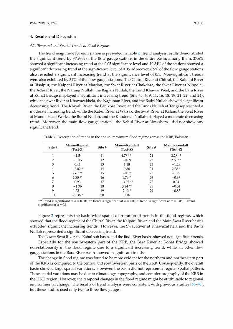
The trend magnitude for each station is presented in Table 2. Trend analysis results demonstratedthe significant trend by 37.93% of the flow gauge stations in the entire basin; among them, 27.6%showed a significant increasing trend at the 0.05 significance level and 10.34% of the stations showed asignificant decreasing trend at the significance level of 0.05. Moreover, 6.9% of the flow gauge stationsalso revealed a significant increasing trend at the significance level of 0.1. Non-significant trendswere also exhibited by 31% of the flow gauge stations. The Chitral River at Chitral, the Kalpani Riverat Risalpur, the Kalpani River at Mardan, the Swat River at Chakdara, the Swat River at Ningolai,the Adezai River, the Naranji Nullah, the Bagiari Nullah, the Lund Khawar West, and the Bara Riverat Kohat Bridge displayed a significant increasing trend (Site #5, 6, 9, 11, 16, 18, 19, 21, 22, and 24),while the Swat River at Khawazakhela, the Naguman River, and the Badri Nullah showed a significantdecreasing trend. The Khiyali River, the Panjkora River, and the Jundi Nullah at Tangi represented amoderate increasing trend, while the Kabul River at Warsak, the Swat River at Kalam, the Swat Riverat Munda Head Works, the Budni Nullah, and the Khuderzai Nullah displayed a moderate decreasingtrend. Moreover, the main flow gauge station—the Kabul River at Nowshera—did not show anysignificant trend.

Table 2. Description of trends in the annual maximum flood regime across the KRB, Pakistan.

Site # Mann–Kendall(Test-Z) Site # Mann–Kendall

(Test-Z) Site # Mann–Kendall(Test-Z)

1 −1.54 11 4.78 *** 21 3.28 **2 −0.35 12 −0.89 22 2.83 **3 0.41 13 1.18 23 −1.284 −2.02 * 14 0.86 24 2.28 *5 2.61 ** 15 −0.37 25 −1.196 2.80 ** 16 1.79 + 26 −0.677 0.93 17 −3.07 ** 27 0.348 −1.36 18 3.24 ** 28 −0.549 1.73 + 19 2.13 * 29 −0.8310 −2.36 * 20 0.16

*** Trend is significant at α = 0.001, ** Trend is significant at α = 0.01, * Trend is significant at α = 0.05, + Trendsignificant at α = 0.1.

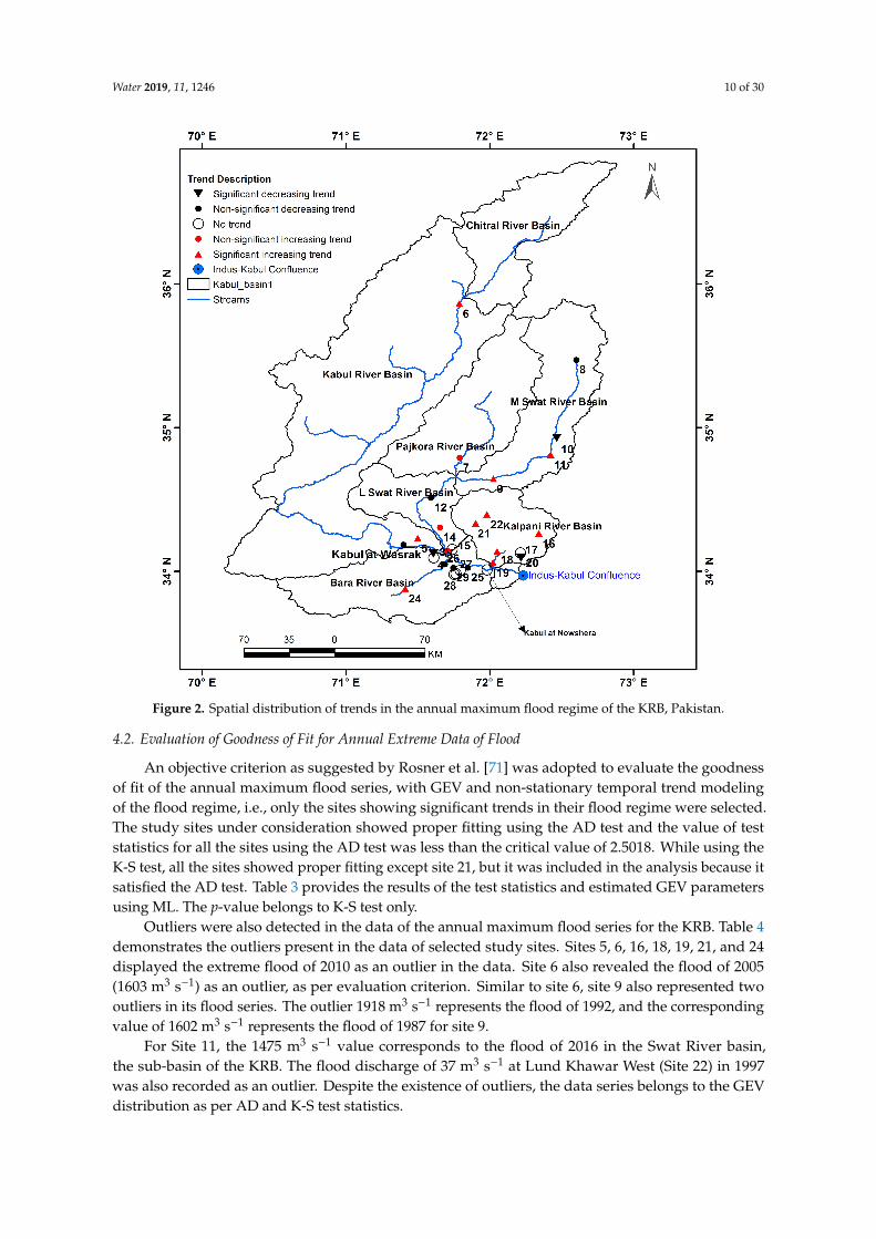
Figure 2 represents the basin-wide spatial distribution of trends in the flood regime, whichshowed that the flood regime of the Chitral River, the Kalpani River, and the Main Swat River basinsexhibited significant increasing trends. However, the Swat River at Khawazakhela and the BadriNullah represented a significant decreasing trend.

The Lower Swat River, the Kabul sub-basin, and the Jindi River basins showed non-significant trends.Especially for the southwestern part of the KRB, the Bara River at Kohat Bridge showed

non-stationarity in the flood regime due to a significant increasing trend, while all other flowgauge stations in the Bara River basin showed insignificant trends.

The change in flood regime was found to be more evident for the northern and northeastern partof the KRB as compared to the central and southwestern parts of the KRB. Consequently, the overallbasin showed large spatial variations. However, the basin did not represent a regular spatial pattern.These spatial variations may be due to climatology, topography, and complex orography of the KRB inthe HKH region. However, the temporal changes in the flood regime might be attributable to regionalenvironmental change. The results of trend analysis were consistent with previous studies [68–70],but these studies used only two to three flow gauges.

Water 2019, 11, 1246 10 of 30Water 2019, 11, x FOR PEER REVIEW 10 of 31

Figure 2. Spatial distribution of trends in the annual maximum flood regime of the KRB, Pakistan.

4.2. Evaluation of Goodness of Fit for Annual Extreme Data of Flood

An objective criterion as suggested by Rosner et al. [71] was adopted to evaluate the goodness of fit of the annual maximum flood series, with GEV and non-stationary temporal trend modeling of the flood regime, i.e., only the sites showing significant trends in their flood regime were selected. The study sites under consideration showed proper fitting using the AD test and the value of test statistics for all the sites using the AD test was less than the critical value of 2.5018. While using the K-S test, all the sites showed proper fitting except site 21, but it was included in the analysis because it satisfied the AD test. Table 3 provides the results of the test statistics and estimated GEV parameters using ML. The p-value belongs to K-S test only.

Outliers were also detected in the data of the annual maximum flood series for the KRB. Table 4 demonstrates the outliers present in the data of selected study sites. Sites 5, 6, 16, 18, 19, 21, and 24 displayed the extreme flood of 2010 as an outlier in the data. Site 6 also revealed the flood of 2005 (1603 m3 s–1) as an outlier, as per evaluation criterion. Similar to site 6, site 9 also represented two outliers in its flood series. The outlier 1918 m3 s–1 represents the flood of 1992, and the corresponding value of 1602 m3 s–1 represents the flood of 1987 for site 9.

For Site 11, the 1475 m3 s–1 value corresponds to the flood of 2016 in the Swat River basin, the sub-basin of the KRB. The flood discharge of 37 m3 s–1 at Lund Khawar West (Site 22) in 1997 was also recorded as an outlier. Despite the existence of outliers, the data series belongs to the GEV distribution as per AD and K-S test statistics.

Figure 2. Spatial distribution of trends in the annual maximum flood regime of the KRB, Pakistan.

4.2. Evaluation of Goodness of Fit for Annual Extreme Data of Flood

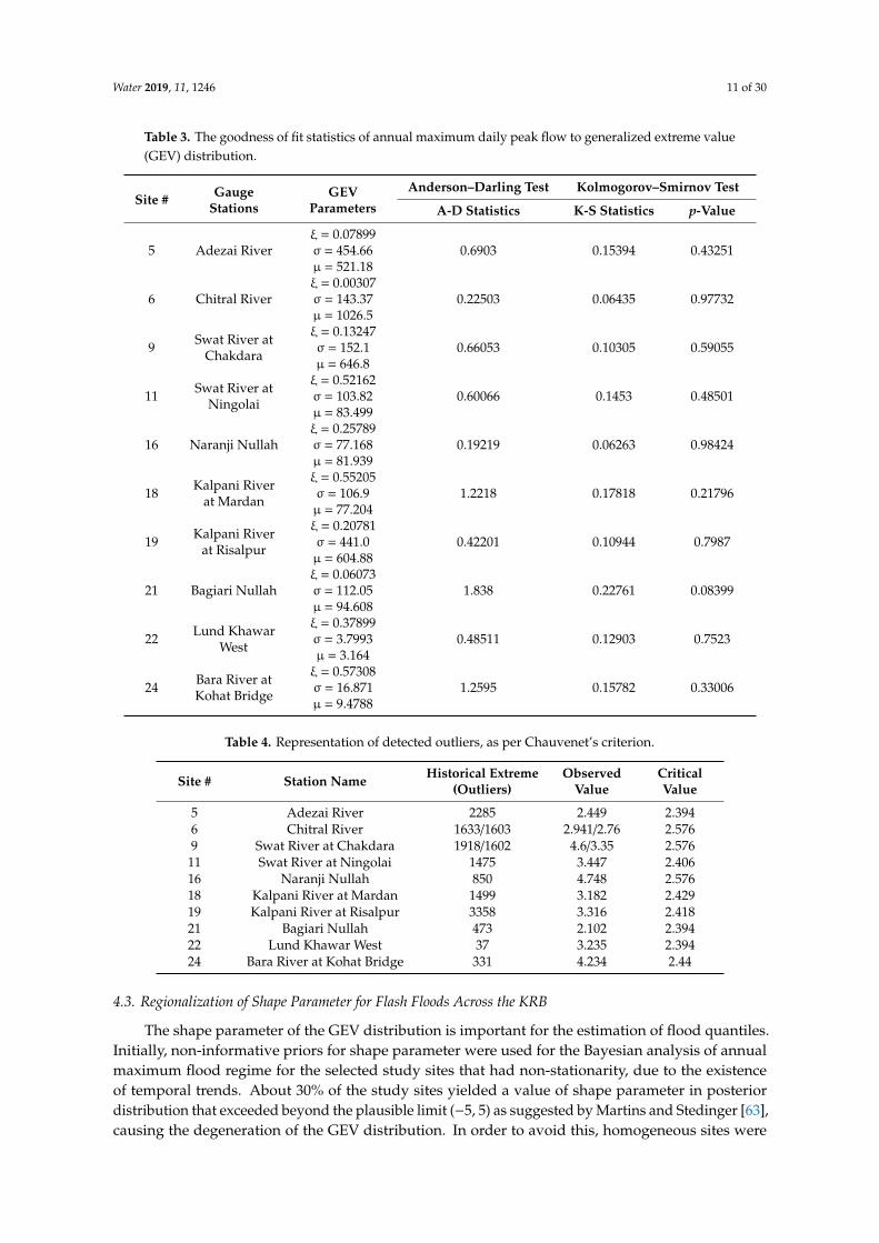
An objective criterion as suggested by Rosner et al. [71] was adopted to evaluate the goodnessof fit of the annual maximum flood series, with GEV and non-stationary temporal trend modelingof the flood regime, i.e., only the sites showing significant trends in their flood regime were selected.The study sites under consideration showed proper fitting using the AD test and the value of teststatistics for all the sites using the AD test was less than the critical value of 2.5018. While using theK-S test, all the sites showed proper fitting except site 21, but it was included in the analysis because itsatisfied the AD test. Table 3 provides the results of the test statistics and estimated GEV parametersusing ML. The p-value belongs to K-S test only.

Outliers were also detected in the data of the annual maximum flood series for the KRB. Table 4demonstrates the outliers present in the data of selected study sites. Sites 5, 6, 16, 18, 19, 21, and 24displayed the extreme flood of 2010 as an outlier in the data. Site 6 also revealed the flood of 2005(1603 m3 s−1) as an outlier, as per evaluation criterion. Similar to site 6, site 9 also represented twooutliers in its flood series. The outlier 1918 m3 s−1 represents the flood of 1992, and the correspondingvalue of 1602 m3 s−1 represents the flood of 1987 for site 9.

For Site 11, the 1475 m3 s−1 value corresponds to the flood of 2016 in the Swat River basin,the sub-basin of the KRB. The flood discharge of 37 m3 s−1 at Lund Khawar West (Site 22) in 1997was also recorded as an outlier. Despite the existence of outliers, the data series belongs to the GEVdistribution as per AD and K-S test statistics.

Water 2019, 11, 1246 11 of 30

Table 3. The goodness of fit statistics of annual maximum daily peak flow to generalized extreme value(GEV) distribution.

Site # GaugeStations

GEVParameters

Anderson–Darling Test Kolmogorov–Smirnov Test

A-D Statistics K-S Statistics p-Value

5 Adezai Riverξ = 0.07899σ = 454.66µ = 521.18

0.6903 0.15394 0.43251

6 Chitral Riverξ = 0.00307σ = 143.37µ = 1026.5

0.22503 0.06435 0.97732

9 Swat River atChakdara

ξ = 0.13247σ = 152.1µ = 646.8

0.66053 0.10305 0.59055

11 Swat River atNingolai

ξ = 0.52162σ = 103.82µ = 83.499

0.60066 0.1453 0.48501

16 Naranji Nullahξ = 0.25789σ = 77.168µ = 81.939

0.19219 0.06263 0.98424

18 Kalpani Riverat Mardan

ξ = 0.55205σ = 106.9µ = 77.204

1.2218 0.17818 0.21796

19 Kalpani Riverat Risalpur

ξ = 0.20781σ = 441.0µ = 604.88

0.42201 0.10944 0.7987

21 Bagiari Nullahξ = 0.06073σ = 112.05µ = 94.608

1.838 0.22761 0.08399

22 Lund KhawarWest

ξ = 0.37899σ = 3.7993µ = 3.164

0.48511 0.12903 0.7523

24 Bara River atKohat Bridge

ξ = 0.57308σ = 16.871µ = 9.4788

1.2595 0.15782 0.33006

Table 4. Representation of detected outliers, as per Chauvenet’s criterion.

Site # Station Name Historical Extreme(Outliers)

ObservedValue

CriticalValue

5 Adezai River 2285 2.449 2.3946 Chitral River 1633/1603 2.941/2.76 2.5769 Swat River at Chakdara 1918/1602 4.6/3.35 2.576

11 Swat River at Ningolai 1475 3.447 2.40616 Naranji Nullah 850 4.748 2.57618 Kalpani River at Mardan 1499 3.182 2.42919 Kalpani River at Risalpur 3358 3.316 2.41821 Bagiari Nullah 473 2.102 2.39422 Lund Khawar West 37 3.235 2.39424 Bara River at Kohat Bridge 331 4.234 2.44

4.3. Regionalization of Shape Parameter for Flash Floods Across the KRB

The shape parameter of the GEV distribution is important for the estimation of flood quantiles.Initially, non-informative priors for shape parameter were used for the Bayesian analysis of annualmaximum flood regime for the selected study sites that had non-stationarity, due to the existenceof temporal trends. About 30% of the study sites yielded a value of shape parameter in posteriordistribution that exceeded beyond the plausible limit (−5, 5) as suggested by Martins and Stedinger [63],causing the degeneration of the GEV distribution. In order to avoid this, homogeneous sites were

Water 2019, 11, 1246 12 of 30

identified. Halbert et al., Kuczera, Kyselý et al., Sun et al., and Viglione et al. [72–76] state that theuse of regional information will improve the flood frequency estimation and reduce the uncertaintyfor sites having short records. Table 5 illustrates the correlation matrix for the selected study sites,which demonstrates that hierarchical clustering is possible based on the correlation between the annualmaximum flood series of the selected study sites.

Table 5. Correlation matrix for the selected study sites.

Site # 5 6 9 11 16 18 19 21 22 24

5 1 0.24 −0.04 0.63 0.35 0.61 0.14 0.25 0.39 0.486 0.24 1 0.29 0.11 0.42 0.33 0.42 0.37 0.38 0.419 −0.04 0.29 1 0.11 0.11 −0.05 −0.22 −0.02 −0.17 0.04

11 0.63 0.11 0.11 1 0.2 0.59 0.04 0.49 0.6 0.2116 0.35 0.42 0.12 0.2 1 0.41 0.47 0.29 0.32 0.6318 0.61 0.33 −0.05 0.59 0.41 1 0.63 0.53 0.52 0.5419 0.14 0.42 −0.22 0.04 0.47 0.63 1 0.65 0.64 0.4221 0.25 0.37 −0.02 0.49 0.29 0.53 0.65 1 0.41 0.222 0.39 0.38 −0.17 0.6 0.32 0.52 0.64 0.41 1 0.4724 0.48 0.41 0.04 0.21 0.63 0.54 0.42 0.2 0.47 1

A positive correlation is present between the sites. Although site 9 possesses the least positivecorrelation with site 6, site 6 has more positive correlations with other sites, hence why all the sites areconsidered homogenous. All the sites also possess “flash” flood type. Moreover, all the sites couldalso be considered homogenous because of the existence of trends in their flood regime. Sun et al. [77]also highlighted the clustering of temporal trends and exchange of shape parameter for the Bayesiananalysis of annual maximum floods across Germany.

Furthermore, the utilization of ML for the estimation of the shape parameter for GEV distributionwas found reliable for large records—at least 50 year [78]. After considering all the study sites ashomogenous based on the correlations between sites, similar flood type, and existence of trends,Naranji Nullah (site 16), with a sufficiently long record, was considered the benchmark site. The shapeparameter estimated by ML was approximately 0.26 for site #16. This value of shape parameter (0.26)was further recognized for all the study sites as an informative prior in the Bayesian model. This is likepartial pooling of information across homogenous sites, which ultimately improved the flood quantilesestimates using the regional information as compared to non-informative priors on shape parameter.Lima et al. [79] used the basin’s average shape parameter value in local and regional hierarchicalBayesian models to solve the issue of sites where the shape parameter value exceeds beyond (−5–5).Lima et al. [79] used the prior for shape parameter as non-informative, but this study considers thepriors on shape parameter to be informative priors.

4.4. Comparison between Stationary and Non-Stationary Bayesian Models

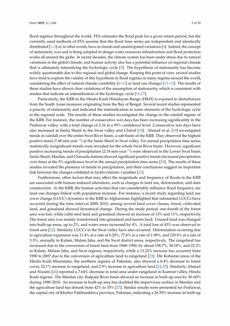
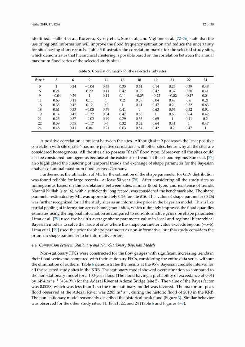
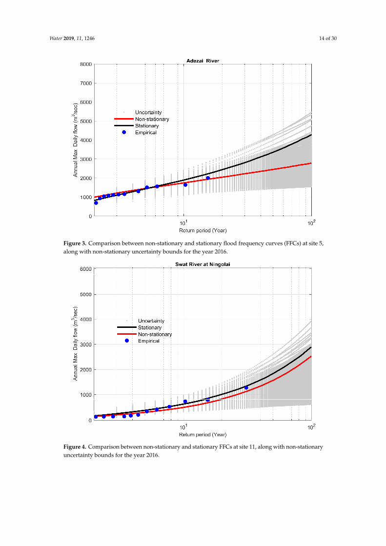
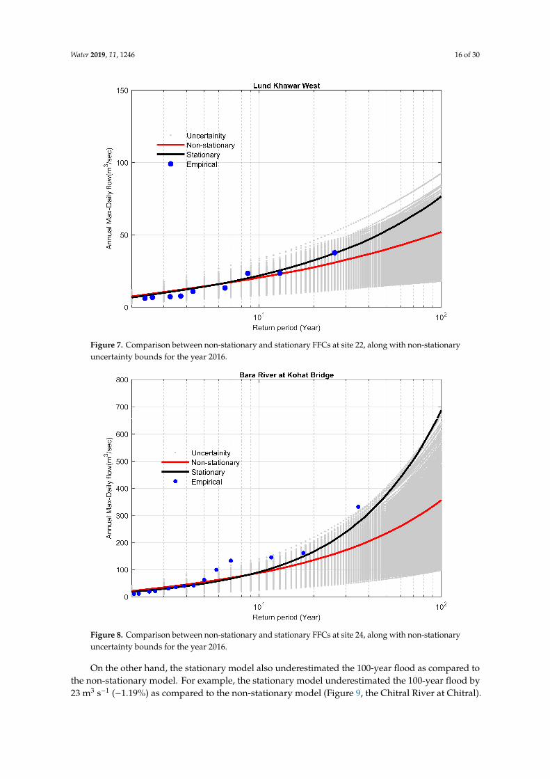
Non-stationary FFCs were constructed for the flow gauges with significant increasing trends intheir flood series and compared with their stationary FFCs, considering the entire data series withoutthe elimination of outliers. Table 6 demonstrates the results at the 95% Bayesian credible interval forall the selected study sites in the KRB. The stationary model showed overestimation as compared tothe non-stationary model for a 100-year flood (The flood having a probability of exceedance of 0.01)by 1494 m3 s−1 (+34.9%) for the Adezai River at Adezai Bridge (site 5). The value of the Bayes factorwas 0.0058, which was less than 1, so the non-stationary model was favored. The maximum peakflood observed at the Adezai River was 2285 m3 s−1, during the historic flood of 2010 in the KRB.The non-stationary model reasonably described the historical peak flood (Figure 3). Similar behaviorwas observed for the other study sites, 11, 18, 21, 22, and 24 (Table 6 and Figures 4–8).

Water 2019, 11, 1246 13 of 30

Table 6. Comparison between 100-year flood estimates using the stationary and non-stationary Bayesian models for “at site modeling” for the KRB, Pakistan.

Site # Station Name HistoricalExtreme m3 s−1

Stationarym3 s−1

Non-Stationarym3 s−1

Difference b/wStationary &

Non-Stationary m3 s−1

PercentDifference (%)

BayesFactor

% Difference betweenPreferred Model and

Historical Extreme

5 Adezai River 2285 4276 2782 1494 34.9 0.0058 17.866 Chitral River 1633 1895 1918 −23 −1.19 0.068 14.859 Swat River at Chakdara 1918 1991 2686 −695 −25.8 7.06 3.8

11 Swat River at Ningolai 1475 2891 2528 363 12.5 0.0065 41.6516 Naranji Nullah 850 1127 1222 −95 −7.7 9.55 24.618 Kalpani River at Mardan 1499 3881 2887 1054 27.15 −Infinity 48.1419 Kalpani River at Risalpur 3358 4918 5140 −222 −4.31 0.4348 34.6621 Bagiari Nullah 473 1666 819 847 50.8 0.0321 42.2422 Lund Khawar West 37 76 51 25 32.89 0.11 27.4524 Bara River at Kohat Bridge 331 686.7 357.5 330.9 48.18 −Infinity 7.2

Water 2019, 11, 1246 14 of 30Water 2019, 11, x FOR PEER REVIEW 0 of 31

Figure 3. Comparison between non-stationary and stationary flood frequency curves (FFCs) at site 5, along with non-stationary uncertainty bounds for the year 2016.

Figure 4. Comparison between non-stationary and stationary FFCs at site 11, along with non-stationary uncertainty bounds for the year 2016.

Figure 3. Comparison between non-stationary and stationary flood frequency curves (FFCs) at site 5,along with non-stationary uncertainty bounds for the year 2016.

Water 2019, 11, x FOR PEER REVIEW 0 of 31

Figure 3. Comparison between non-stationary and stationary flood frequency curves (FFCs) at site 5, along with non-stationary uncertainty bounds for the year 2016.

Figure 4. Comparison between non-stationary and stationary FFCs at site 11, along with non-stationary uncertainty bounds for the year 2016.

Figure 4. Comparison between non-stationary and stationary FFCs at site 11, along with non-stationaryuncertainty bounds for the year 2016.

Water 2019, 11, 1246 15 of 30Water 2019, 11, x FOR PEER REVIEW 1 of 31

Figure 5. Comparison between non-stationary and stationary FFCs at site 18, along with non-stationary uncertainty bounds for the year 2016.

Figure 6. Comparison between non-stationary and stationary FFCs at site 21, along with non-stationary uncertainty bounds for the year 2016.

Figure 5. Comparison between non-stationary and stationary FFCs at site 18, along with non-stationaryuncertainty bounds for the year 2016.

Water 2019, 11, x FOR PEER REVIEW 1 of 31

Figure 5. Comparison between non-stationary and stationary FFCs at site 18, along with non-stationary uncertainty bounds for the year 2016.

Figure 6. Comparison between non-stationary and stationary FFCs at site 21, along with non-stationary uncertainty bounds for the year 2016.

Figure 6. Comparison between non-stationary and stationary FFCs at site 21, along with non-stationaryuncertainty bounds for the year 2016.

Water 2019, 11, 1246 16 of 30Water 2019, 11, x FOR PEER REVIEW 2 of 31

Figure 7. Comparison between non-stationary and stationary FFCs at site 22, along with non-stationary uncertainty bounds for the year 2016.

Figure 8. Comparison between non-stationary and stationary FFCs at site 24, along with non-stationary uncertainty bounds for the year 2016.

Figure 7. Comparison between non-stationary and stationary FFCs at site 22, along with non-stationaryuncertainty bounds for the year 2016.

Water 2019, 11, x FOR PEER REVIEW 2 of 31

Figure 7. Comparison between non-stationary and stationary FFCs at site 22, along with non-stationary uncertainty bounds for the year 2016.

Figure 8. Comparison between non-stationary and stationary FFCs at site 24, along with non-stationary uncertainty bounds for the year 2016.

Figure 8. Comparison between non-stationary and stationary FFCs at site 24, along with non-stationaryuncertainty bounds for the year 2016.

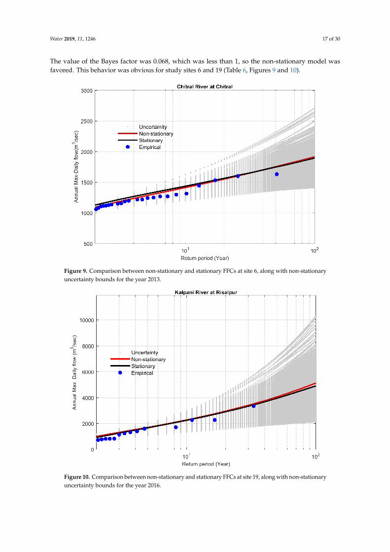
On the other hand, the stationary model also underestimated the 100-year flood as compared tothe non-stationary model. For example, the stationary model underestimated the 100-year flood by23 m3 s−1 (−1.19%) as compared to the non-stationary model (Figure 9, the Chitral River at Chitral).

Water 2019, 11, 1246 17 of 30

The value of the Bayes factor was 0.068, which was less than 1, so the non-stationary model wasfavored. This behavior was obvious for study sites 6 and 19 (Table 6, Figures 9 and 10).

Water 2019, 11, x FOR PEER REVIEW 3 of 31

Figure 9. Comparison between non-stationary and stationary FFCs at site 6, along with non-stationary uncertainty bounds for the year 2013.

Figure 10. Comparison between non-stationary and stationary FFCs at site 19, along with non-stationary uncertainty bounds for the year 2016.

Figure 9. Comparison between non-stationary and stationary FFCs at site 6, along with non-stationaryuncertainty bounds for the year 2013.

Water 2019, 11, x FOR PEER REVIEW 3 of 31

Figure 9. Comparison between non-stationary and stationary FFCs at site 6, along with non-stationary uncertainty bounds for the year 2013.

Figure 10. Comparison between non-stationary and stationary FFCs at site 19, along with non-stationary uncertainty bounds for the year 2016.

Figure 10. Comparison between non-stationary and stationary FFCs at site 19, along with non-stationaryuncertainty bounds for the year 2016.

Water 2019, 11, 1246 18 of 30

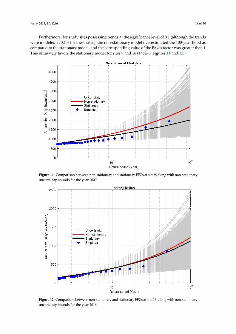
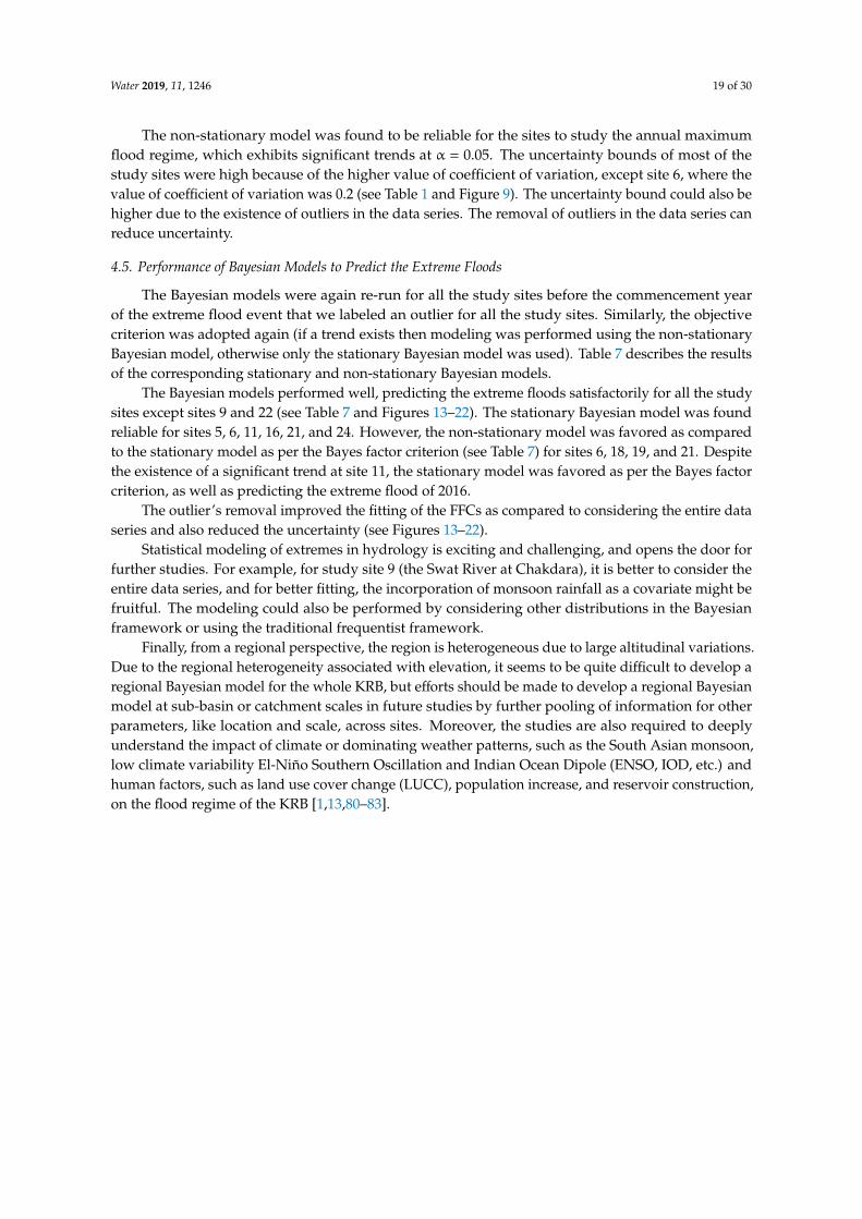
Furthermore, for study sites possessing trends at the significance level of 0.1 (although the trendswere modeled at 0.1% for these sites), the non-stationary model overestimated the 100-year flood ascompared to the stationary model, and the corresponding value of the Bayes factor was greater than 1.This ultimately favors the stationary model for sites 9 and 16 (Table 6, Figures 11 and 12).

Water 2019, 11, x FOR PEER REVIEW 4 of 31

Figure 11. Comparison between non-stationary and stationary FFCs at site 9, along with non-stationary uncertainty bounds for the year 2009.

Figure 12. Comparison between non-stationary and stationary FFCs at site 16, along with non-stationary uncertainty bounds for the year 2016.

The non-stationary model was found to be reliable for the sites to study the annual maximum flood regime, which exhibits significant trends at α = 0.05. The uncertainty bounds of most of the

Figure 11. Comparison between non-stationary and stationary FFCs at site 9, along with non-stationaryuncertainty bounds for the year 2009.

Water 2019, 11, x FOR PEER REVIEW 4 of 31

Figure 11. Comparison between non-stationary and stationary FFCs at site 9, along with non-stationary uncertainty bounds for the year 2009.

Figure 12. Comparison between non-stationary and stationary FFCs at site 16, along with non-stationary uncertainty bounds for the year 2016.

The non-stationary model was found to be reliable for the sites to study the annual maximum flood regime, which exhibits significant trends at α = 0.05. The uncertainty bounds of most of the

Figure 12. Comparison between non-stationary and stationary FFCs at site 16, along with non-stationaryuncertainty bounds for the year 2016.

Water 2019, 11, 1246 19 of 30

The non-stationary model was found to be reliable for the sites to study the annual maximumflood regime, which exhibits significant trends at α = 0.05. The uncertainty bounds of most of thestudy sites were high because of the higher value of coefficient of variation, except site 6, where thevalue of coefficient of variation was 0.2 (see Table 1 and Figure 9). The uncertainty bound could also behigher due to the existence of outliers in the data series. The removal of outliers in the data series canreduce uncertainty.

4.5. Performance of Bayesian Models to Predict the Extreme Floods

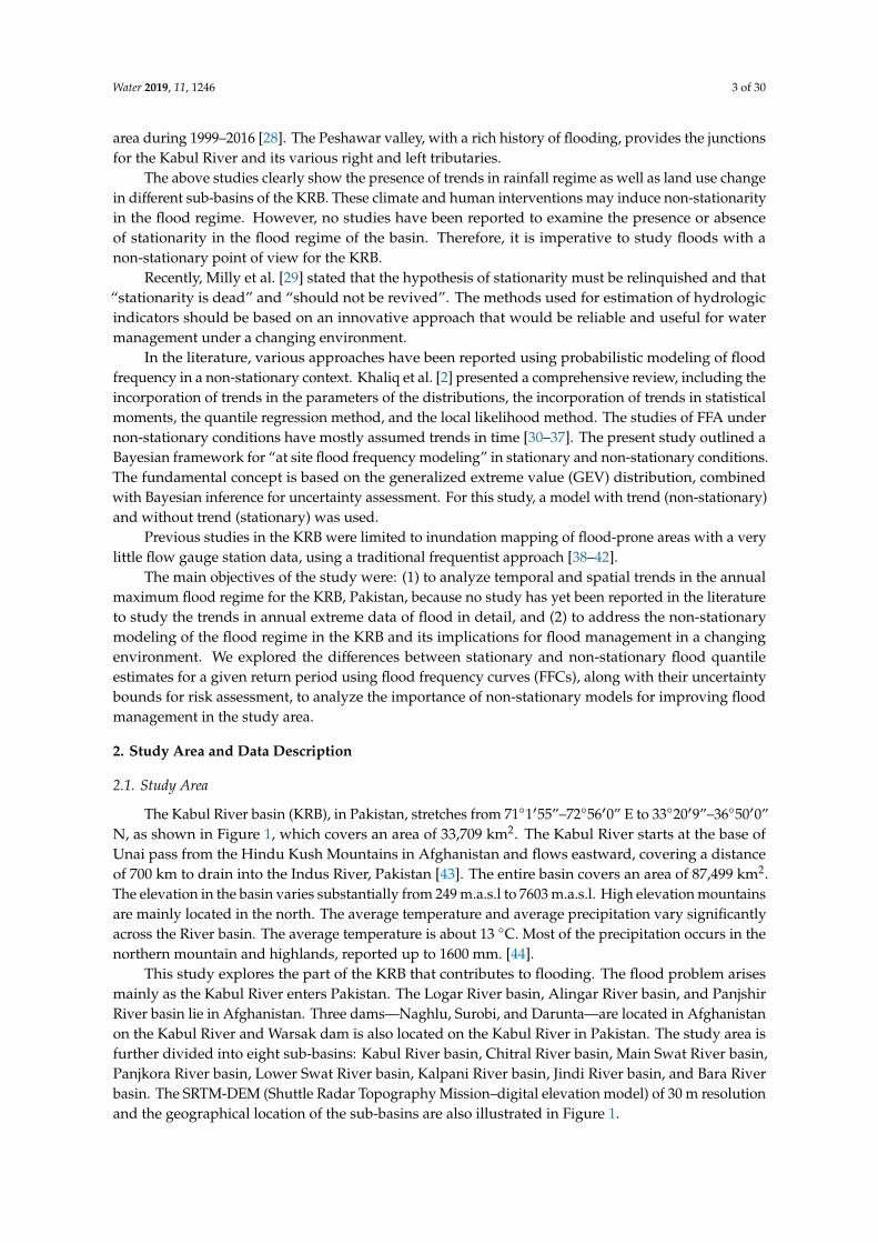
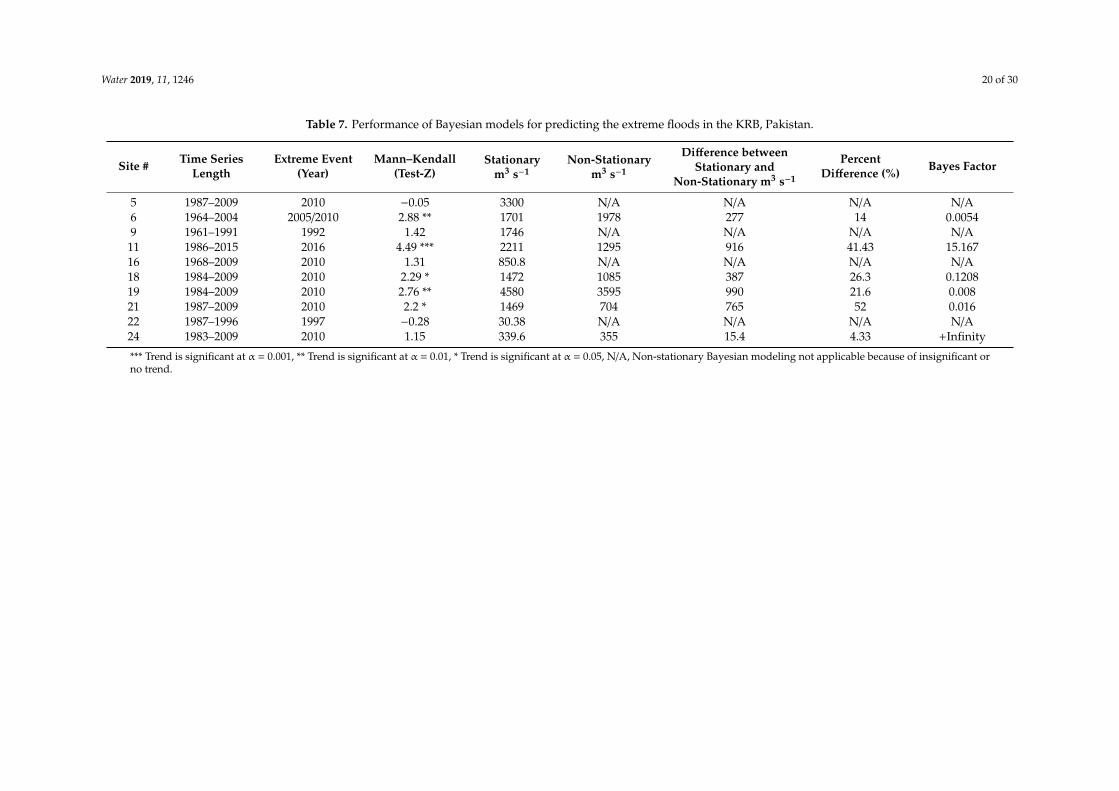
The Bayesian models were again re-run for all the study sites before the commencement yearof the extreme flood event that we labeled an outlier for all the study sites. Similarly, the objectivecriterion was adopted again (if a trend exists then modeling was performed using the non-stationaryBayesian model, otherwise only the stationary Bayesian model was used). Table 7 describes the resultsof the corresponding stationary and non-stationary Bayesian models.

The Bayesian models performed well, predicting the extreme floods satisfactorily for all the studysites except sites 9 and 22 (see Table 7 and Figures 13–22). The stationary Bayesian model was foundreliable for sites 5, 6, 11, 16, 21, and 24. However, the non-stationary model was favored as comparedto the stationary model as per the Bayes factor criterion (see Table 7) for sites 6, 18, 19, and 21. Despitethe existence of a significant trend at site 11, the stationary model was favored as per the Bayes factorcriterion, as well as predicting the extreme flood of 2016.

The outlier’s removal improved the fitting of the FFCs as compared to considering the entire dataseries and also reduced the uncertainty (see Figures 13–22).

Statistical modeling of extremes in hydrology is exciting and challenging, and opens the door forfurther studies. For example, for study site 9 (the Swat River at Chakdara), it is better to consider theentire data series, and for better fitting, the incorporation of monsoon rainfall as a covariate might befruitful. The modeling could also be performed by considering other distributions in the Bayesianframework or using the traditional frequentist framework.

Finally, from a regional perspective, the region is heterogeneous due to large altitudinal variations.Due to the regional heterogeneity associated with elevation, it seems to be quite difficult to develop aregional Bayesian model for the whole KRB, but efforts should be made to develop a regional Bayesianmodel at sub-basin or catchment scales in future studies by further pooling of information for otherparameters, like location and scale, across sites. Moreover, the studies are also required to deeplyunderstand the impact of climate or dominating weather patterns, such as the South Asian monsoon,low climate variability El-Niño Southern Oscillation and Indian Ocean Dipole (ENSO, IOD, etc.) andhuman factors, such as land use cover change (LUCC), population increase, and reservoir construction,on the flood regime of the KRB [1,13,80–83].

Water 2019, 11, 1246 20 of 30

Table 7. Performance of Bayesian models for predicting the extreme floods in the KRB, Pakistan.

Site # Time SeriesLength

Extreme Event(Year)

Mann–Kendall(Test-Z)

Stationarym3 s−1

Non-Stationarym3 s−1

Difference betweenStationary and

Non-Stationary m3 s−1

PercentDifference (%) Bayes Factor

5 1987–2009 2010 −0.05 3300 N/A N/A N/A N/A6 1964–2004 2005/2010 2.88 ** 1701 1978 277 14 0.00549 1961–1991 1992 1.42 1746 N/A N/A N/A N/A

11 1986–2015 2016 4.49 *** 2211 1295 916 41.43 15.16716 1968–2009 2010 1.31 850.8 N/A N/A N/A N/A18 1984–2009 2010 2.29 * 1472 1085 387 26.3 0.120819 1984–2009 2010 2.76 ** 4580 3595 990 21.6 0.00821 1987–2009 2010 2.2 * 1469 704 765 52 0.01622 1987–1996 1997 −0.28 30.38 N/A N/A N/A N/A24 1983–2009 2010 1.15 339.6 355 15.4 4.33 +Infinity

*** Trend is significant at α = 0.001, ** Trend is significant at α = 0.01, * Trend is significant at α = 0.05, N/A, Non-stationary Bayesian modeling not applicable because of insignificant orno trend.

Water 2019, 11, 1246 21 of 30Water 2019, 11, x FOR PEER REVIEW 0 of 31

Figure 13. FFCs at site 5, along with stationary uncertainty bounds for the year 2009.

Figure 14. Comparison between non-stationary and stationary FFCs at site 6, along with non-stationary uncertainty bounds for the year 2004.

Figure 13. FFCs at site 5, along with stationary uncertainty bounds for the year 2009.

Water 2019, 11, x FOR PEER REVIEW 0 of 31

Figure 13. FFCs at site 5, along with stationary uncertainty bounds for the year 2009.

Figure 14. Comparison between non-stationary and stationary FFCs at site 6, along with non-stationary uncertainty bounds for the year 2004.

Figure 14. Comparison between non-stationary and stationary FFCs at site 6, along with non-stationaryuncertainty bounds for the year 2004.

Water 2019, 11, 1246 22 of 30Water 2019, 11, x FOR PEER REVIEW 1 of 31

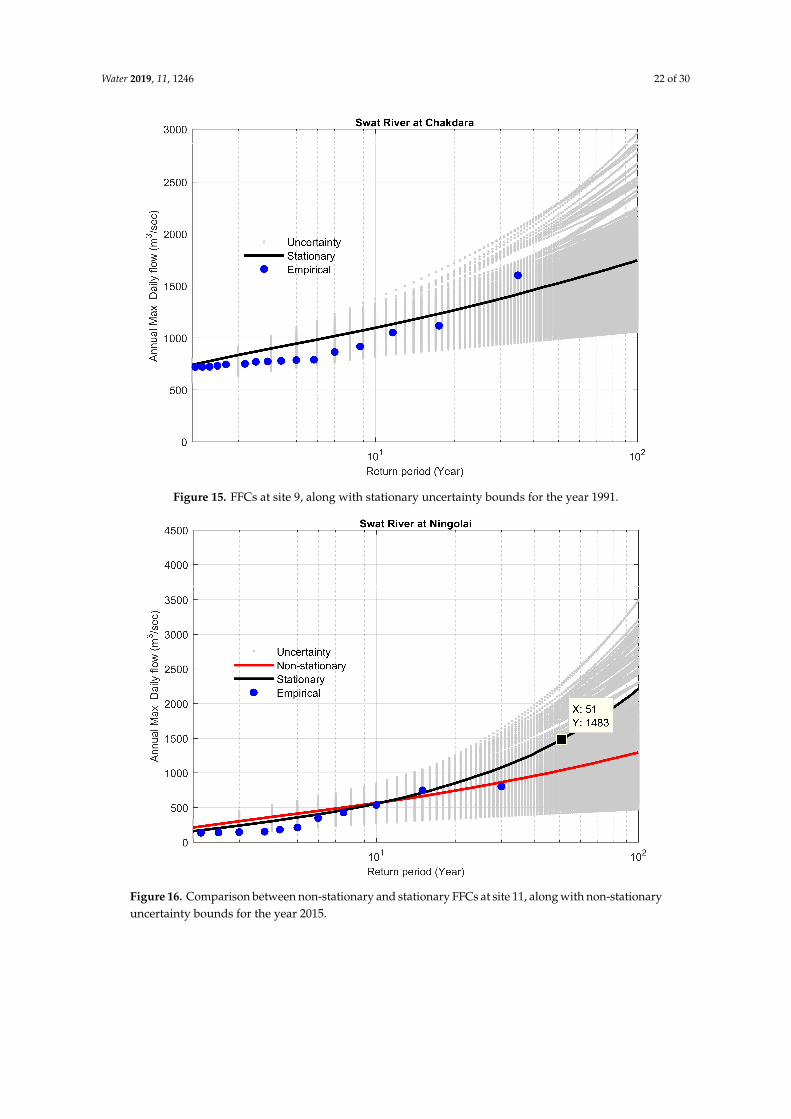
Figure 15. FFCs at site 9, along with stationary uncertainty bounds for the year 1991.

Figure 16. Comparison between non-stationary and stationary FFCs at site 11, along with non-stationary uncertainty bounds for the year 2015.

Figure 15. FFCs at site 9, along with stationary uncertainty bounds for the year 1991.

Water 2019, 11, x FOR PEER REVIEW 1 of 31

Figure 15. FFCs at site 9, along with stationary uncertainty bounds for the year 1991.

Figure 16. Comparison between non-stationary and stationary FFCs at site 11, along with non-stationary uncertainty bounds for the year 2015.

Figure 16. Comparison between non-stationary and stationary FFCs at site 11, along with non-stationaryuncertainty bounds for the year 2015.

Water 2019, 11, 1246 23 of 30Water 2019, 11, x FOR PEER REVIEW 2 of 31

Figure 17. FFCs at site 16, along with stationary uncertainty bounds for the year 2009.

Figure 18. Comparison between non-stationary and stationary FFCs at site 18, along with non-stationary uncertainty bounds for the year 2009.

Figure 17. FFCs at site 16, along with stationary uncertainty bounds for the year 2009.

Water 2019, 11, x FOR PEER REVIEW 2 of 31

Figure 17. FFCs at site 16, along with stationary uncertainty bounds for the year 2009.

Figure 18. Comparison between non-stationary and stationary FFCs at site 18, along with non-stationary uncertainty bounds for the year 2009.

Figure 18. Comparison between non-stationary and stationary FFCs at site 18, along with non-stationaryuncertainty bounds for the year 2009.

Water 2019, 11, 1246 24 of 30Water 2019, 11, x FOR PEER REVIEW 3 of 31

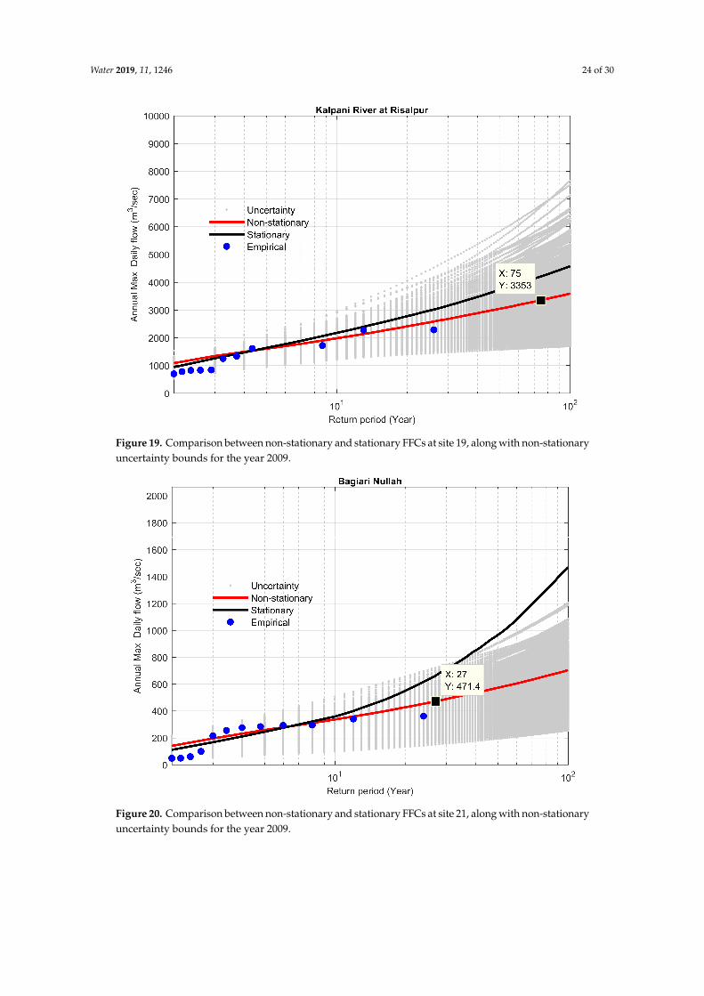
Figure 19. Comparison between non-stationary and stationary FFCs at site 19, along with non-stationary uncertainty bounds for the year 2009.

Figure 20. Comparison between non-stationary and stationary FFCs at site 21, along with non-stationary uncertainty bounds for the year 2009.

Figure 19. Comparison between non-stationary and stationary FFCs at site 19, along with non-stationaryuncertainty bounds for the year 2009.

Water 2019, 11, x FOR PEER REVIEW 3 of 31

Figure 19. Comparison between non-stationary and stationary FFCs at site 19, along with non-stationary uncertainty bounds for the year 2009.

Figure 20. Comparison between non-stationary and stationary FFCs at site 21, along with non-stationary uncertainty bounds for the year 2009.

Figure 20. Comparison between non-stationary and stationary FFCs at site 21, along with non-stationaryuncertainty bounds for the year 2009.

Water 2019, 11, 1246 25 of 30Water 2019, 11, x FOR PEER REVIEW 4 of 31

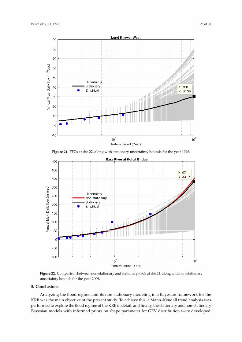
Figure 21. FFCs at site 22, along with stationary uncertainty bounds for the year 1996.

Figure 22. Comparison between non-stationary and stationary FFCs at site 24, along with non-stationary uncertainty bounds for the year 2009.

Statistical modeling of extremes in hydrology is exciting and challenging, and opens the door for further studies. For example, for study site 9 (the Swat River at Chakdara), it is better to consider the entire data series, and for better fitting, the incorporation of monsoon rainfall as a covariate might

Figure 21. FFCs at site 22, along with stationary uncertainty bounds for the year 1996.

Water 2019, 11, x FOR PEER REVIEW 4 of 31

Figure 21. FFCs at site 22, along with stationary uncertainty bounds for the year 1996.

Figure 22. Comparison between non-stationary and stationary FFCs at site 24, along with non-stationary uncertainty bounds for the year 2009.

Statistical modeling of extremes in hydrology is exciting and challenging, and opens the door for further studies. For example, for study site 9 (the Swat River at Chakdara), it is better to consider the entire data series, and for better fitting, the incorporation of monsoon rainfall as a covariate might

Figure 22. Comparison between non-stationary and stationary FFCs at site 24, along with non-stationaryuncertainty bounds for the year 2009.

5. Conclusions

Analyzing the flood regime and its non-stationary modeling in a Bayesian framework for theKRB was the main objective of the present study. To achieve this, a Mann–Kendall trend analysis wasperformed to explore the flood regime of the KRB in detail, and finally, the stationary and non-stationaryBayesian models with informed priors on shape parameter for GEV distribution were developed,

Water 2019, 11, 1246 26 of 30

and their results were compared by using the corresponding FFCs, along with their uncertainty bounds.We utilized the annual extreme data of flood series for the study area, with a maximum record of1962–2016 (55 years) and a minimum of 1987–2016 (30 years). The key findings of the study aredescribed below:

1. Trend analysis showed a mixture of increasing and decreasing trends at different gauges in theKRB at α = 0.05. The Chitral River, Kalpani River, Main Swat River, and Bara River basins showedsignificant increasing trends, and the Panjkora River basin displayed a moderate increasing trendin its annual maximum flood regime. However, the Lower Swat and Kabul sub-basins showeddecreasing trends, except for the Adezai River in the Kabul sub-basin, which showed a significantincreasing trend.

2. The overall basin was under critical change and signals of clear non-stationarity in the floodregime were evident at various spatial scales throughout the basin.

3. The presence of a significant trend and significant difference in flood estimates for 100-year floodbetween stationary and non-stationary FFCs were found that represent the clear violation fromthe so-called stationary assumption.

4. The non-stationary Bayesian model was found to be reliable for the study sites that had asignificant trend at α = 0.05, while the stationary model overestimated or underestimated theflood risk for these sites. On the other hand, the stationary Bayesian model performed better forthe study sites for trends at α = 0.1, while the non-stationary Bayesian model overestimated orunderestimated the flood risk for such sites.

5. The use of informed priors on the shape parameter based on regional information improved theestimation of flood quantiles and reduced the uncertainty.

6. Proper consideration should be given to identify the outliers while using Bayesian models.7. The presence of non-stationarity in the flood regime of the KRB has substantial implications for

flood management and water resources development. A design with stationary assumptionwill cause two major concerns: under estimation or overestimation of design for structuraland non-structural measures in the KRB. An event-based design may also overestimate orunderestimate the risk in hydraulic design that was intended. Some previous studies in otherparts of world also provided similar results [1,13,31,84–86].

The study will be helpful for sustainable flood management and provide a reference for studyingfloods in a changing environment for hydrologists, water resources managers, decision makers,and concerned organizations.

Author Contributions: This research article, A.M. and S.J. formulated research design, plan, organized researchflow and manuscript write up. A.M. performed analysis, S.J. supervised research work and contributed in theinterpretation of results and discussions, R.M. and M.A. contributed in drafting and map preparations and J.Y.was involved in short listing data sets from 45 flow gauge stations to 29 for the current study. All the authorscontributed well to writing at various stages.

Funding: This research was funded by CAS-TWAS President Fellowship Program for doctoral students and theStrategic Priority Research Program of the Chinese Academy of Sciences [XDA20010201].

Acknowledgments: The authors acknowledge SWHP (Surface Water Hydrology Project) WAPDA Pakistan andIrrigation Department Khyber Pakhtunkhwa, Pakistan to provide data for this study.

Conflicts of Interest: The authors declare no conflicts of interests.

References

1. López, J.; Francés, F. Non-stationary flood frequency analysis in continental Spanish rivers, using climateand reservoir indices as external covariates. Hydrol. Earth Syst. Sci. 2013, 17, 3189–3203. [CrossRef]

2. Khaliq, M.; Ouarda, T.; Ondo, J.-C.; Gachon, P.; Bobée, B. Frequency analysis of a sequence of dependentand/or non-stationary hydro-meteorological observations: A review. J. Hydrol. 2006, 329, 534–552. [CrossRef]

Water 2019, 11, 1246 27 of 30

3. Stedinger, J.R.; Vogel, R.; Foufoula-Georgiou, E. Frequency analysis of extreme events. Handb. Hydrol. 1993,18, 68.

4. Salas, J. Analysis and Modeling of Hydrologic Time Series in Hand Book of Hydrology; Maidment, D.R., Ed.;McGraw Hill Book Co.: New York, NY, USA, 1993.

5. Council, N.R. Decade-to-Century-Scale Climate Variability and Change: A Science Strategy; National AcademiesPress: Washington, DC, USA, 1998.

6. Norrant, C.; Douguédroit, A. Monthly and daily precipitation trends in the Mediterranean (1950–2000).Theor. Appl. Climatol. 2006, 83, 89–106. [CrossRef]

7. Mudelsee, M.; Börngen, M.; Tetzlaff, G.; Grünewald, U. No upward trends in the occurrence of extremefloods in central Europe. Nature 2003, 425, 166–169. [CrossRef]

8. Douglas, E.; Vogel, R.; Kroll, C. Trends in floods and low flows in the United States: Impact of spatialcorrelation. J. Hydrol. 2000, 240, 90–105. [CrossRef]

9. Franks, S.W. Identification of a change in climate state using regional flood data. Hydrol. Earth Syst. Sci.2002, 6, 11–16. [CrossRef]

10. Milly, P.C.; Dunne, K.A.; Vecchia, A.V. Global pattern of trends in streamflow and water availability in achanging climate. Nature 2005, 438, 347–350. [CrossRef]

11. Villarini, G.; Serinaldi, F.; Smith, J.A.; Krajewski, W.F. On the stationarity of annual flood peaks in thecontinental united states during the 20th century. Water Resour. Res. 2009, 45. [CrossRef]

12. Wilson, D.; Hisdal, H.; Lawrence, D. Has streamflow changed in the nordic countries?–recent trends andcomparisons to hydrological projections. J. Hydrol. 2010, 394, 334–346. [CrossRef]

13. Villarini, G.; Smith, J.A.; Serinaldi, F.; Bales, J.; Bates, P.D.; Krajewski, W.F. Flood frequency analysis fornonstationary annual peak records in an urban drainage basin. Adv. Water Resour. 2009, 32, 1255–1266.[CrossRef]

14. Vogel, R.M.; Yaindl, C.; Walter, M. Nonstationarity: Flood magnification and recurrence reduction factors inthe United States. J. Am. Water Resour. Assoc. 2011, 47, 464–474. [CrossRef]

15. Hejazi, M.I.; Markus, M. Impacts of urbanization and climate variability on floods in northeastern Illinois.J. Hydrol. Eng. 2009, 14, 606–616. [CrossRef]

16. Held, I.M.; Soden, B.J. Robust responses of the hydrological cycle to global warming. J. Clim. 2006, 19,5686–5699. [CrossRef]

17. Allen, M.R.; Smith, L.A. Monte carlo ssa: Detecting irregular oscillations in the presence of colored noise.J. Clim. 1996, 9, 3373–3404. [CrossRef]

18. Zaman, C.Q.U.; Mahmood, A.; Rasul, G.; Afzal, M. Climate Change Indicators of Pakistan; Report No:PMD-22/2009; Pakistan Meteorological Department: Islamabad, Pakistan, 2009.

19. Ahmad, I.; Tang, D.; Wang, T.; Wang, M.; Wagan, B. Precipitation trends over time using mann-kendall andspearman’s rho tests in Swat river basin, Pakistan. Adv. Meteorol. 2015, 2015, 431860. [CrossRef]

20. Khalid, S.; Rehman, S.U.; Shah, S.M.A.; Naz, A.; Saeed, B.; Alam, S.; Ali, F.; Gul, H. Hydro-meteorologicalcharacteristics of Chitral river basin at the peak of the Hindukush range. Nat. Sci. 2013, 5, 987. [CrossRef]

21. Hartmann, H.; Buchanan, H. Trends in extreme precipitation events in the Indus river basin and flooding inPakistan. Atmos. Ocean 2014, 52, 77–91. [CrossRef]

22. Najmuddin, O.; Deng, X.; Siqi, J. Scenario analysis of land use change in Kabul river basin–a river basin withrapid socio-economic changes in Afghanistan. Phys. Chem. Earth Parts A B C 2017, 101, 121–136. [CrossRef]

23. Qasim, M.; Hubacek, K.; Termansen, M.; Khan, A. Spatial and temporal dynamics of land use pattern indistrict Swat, Hindu Kush Himalayan region of Pakistan. Appl. Geogr. 2011, 31, 820–828. [CrossRef]

24. Ullah, S.; Farooq, M.; Shafique, M.; Siyab, M.A.; Kareem, F.; Dees, M. Spatial assessment of forest cover andland-use changes in the Hindu-Kush mountain ranges of northern Pakistan. J. Mt. Sci. 2016, 13, 1229–1237.[CrossRef]

25. Sajjad, A.; Adnan, S.; Hussain, A. Forest land cover change from year 2000 to 2012 of tehsil Barawal DirUpper Pakistan. Int. J. Adv. Res. Biol. Sci. 2016, 3, 144–154.

26. Ahmad, A.; Nizami, S.M. Carbon stocks of different land uses in the Kumrat valley, Hindu Kush region ofPakistan. J. For. Res. 2015, 26, 57–64. [CrossRef]

27. Yar, P.; Atta-ur-Rahman, M.A.K.; Samiullah, S. Spatio-temporal analysis of urban expansion on farmland andits impact on the agricultural land use of Mardan city, Pakistan. Proc. Pak. Acad. Sci. B Life Environ. Sci. 2016,53, 35–46.

Water 2019, 11, 1246 28 of 30

28. Raziq, A.; Xu, A.; Li, Y.; Zhao, Q. Monitoring of land use/land cover changes and urban sprawl in peshawarcity in khyber pakhtunkhwa: An application of geo-information techniques using of multi-temporal satellitedata. J. Remote Sens. GIS 2016, 5. [CrossRef]

29. Milly, P.C.; Betancourt, J.; Falkenmark, M.; Hirsch, R.M.; Kundzewicz, Z.W.; Lettenmaier, D.P.; Stouffer, R.J.Stationarity is dead: Whither water management? Science 2008, 319, 573–574. [CrossRef] [PubMed]

30. Delgado, J.M.; Apel, H.; Merz, B. Flood trends and variability in the Mekong river. Hydrol. Earth Syst. Sci.2010, 14, 407–418. [CrossRef]

31. Leclerc, M.; Ouarda, T.B. Non-stationary regional flood frequency analysis at ungauged sites. J. Hydrol. 2007,343, 254–265. [CrossRef]

32. Olsen, J.R.; Lambert, J.H.; Haimes, Y.Y. Risk of extreme events under nonstationary conditions. Risk Anal.1998, 18, 497–510. [CrossRef]

33. McNeil, A.J.; Saladin, T. Developing Scenarios for Future Extreme Losses Using the Pot Method. In Extremesand Integrated Risk Management; Embrechts, P., Ed.; CiteseerX: Zurich, Switzerland, 2000; pp. 253–267.

34. Stedinger, J.R.; Crainiceanu, C.M. Climate Variability and Flood-Risk Management. In Risk-Based DecisionMaking in Water Resources IX; ASCE: Reston, VA, USA, 2001; pp. 77–86.

35. Strupczewski, W.; Singh, V.; Mitosek, H. Non-stationary approach to at-site flood frequency modelling. III.Flood analysis of Polish rivers. J. Hydrol. 2001, 248, 152–167. [CrossRef]

36. He, Y.; Bárdossy, A.; Brommundt, J. Non-Stationary Flood Frequency Analysis in Southern Germany.In Proceedings of the Seventh International Conference on Hydroscience and Engineering, Philadelphia, PA,USA, 10–13 September 2006.

37. Renard, B.; Lang, M.; Bois, P. Statistical analysis of extreme events in a non-stationary context via a bayesianframework: Case study with peak-over-threshold data. Stoch. Environ. Res. Risk Assess. 2006, 21, 97–112.[CrossRef]

38. Khattak, M.; Anwar, F.; Sheraz, K.; Saeed, T.; Sharif, M.; Ahmed, A. Floodplain mapping using hec-ras andarcgis: A case study of Kabul river. Arab. J. Sci. Eng. (Springer Sci. Bus. Media BV) 2016, 41, 1375–1390.[CrossRef]

39. Sayama, T.; Ozawa, G.; Kawakami, T.; Nabesaka, S.; Fukami, K. Rainfall–runoff–inundation analysis of the2010 Pakistan flood in the Kabul river basin. Hydrol. Sci. J. 2012, 57, 298–312. [CrossRef]

40. Bahadar, I.; Shafique, M.; Khan, T.; Tabassum, I.; Ali, M.Z. Flood hazard assessment using hydro-dynamicmodel and gis/rs tools: A case study of Babuzai-Kabal tehsil Swat basin, Pakistan. J. Himal. Earth Sci. 2015,48, 129–138.

41. Aziz, A. Rainfall-runoff modeling of the trans-boundary Kabul river basin using integrated flood analysissystem (ifas). Pak. J. Meteorol. 2014, 10, 75–81.

42. Ullah, S.; Farooq, M.; Sarwar, T.; Tareen, M.J.; Wahid, M.A. Flood modeling and simulations usinghydrodynamic model and aster dem—A case study of Kalpani river. Arab. J. Geosci. 2016, 9, 439. [CrossRef]

43. Mack, T.J.; Chornack, M.P.; Taher, M.R. Groundwater-level trends and implications for sustainable water usein the Kabul basin, afghanistan. Environ. Syst. Decis. 2013, 33, 457–467. [CrossRef]

44. Lashkaripour, G.R.; Hussaini, S. Water resource management in Kabul river basin, Eastern Afghanistan.Environmentalist 2008, 28, 253–260. [CrossRef]

45. Tariq, M.A.U.R.; Van de Giesen, N. Floods and flood management in Pakistan. Phys. Chem. Earth Parts A B C2012, 47, 11–20. [CrossRef]

46. Anjum, M.N.; Ding, Y.; Shangguan, D.; Ijaz, M.W.; Zhang, S. Evaluation of high-resolution satellite-basedreal-time and post-real-time precipitation estimates during 2010 extreme flood event in Swat river basin,Hindukush region. Adv. Meteorol. 2016, 2016, 2604980. [CrossRef]

47. Rasul, G.; Dahe, Q.; Chaudhry, Q. Global warming and melting glaciers along southern slopes of HKH range.Pak. J. Meteorol. 2008, 5, 63–76.

48. Mann, H.B. Nonparametric tests against trend. Econom. J. Econom. Soc. 1945, 13, 245–259. [CrossRef]49. Kendall, M. Rank Correlation Methods; Charles Griffin: London, UK, 1975.50. Katz, R.W. Statistics of extremes in climate change. Clim. Chang. 2010, 100, 71–76. [CrossRef]51. Coles, S.; Bawa, J.; Trenner, L.; Dorazio, P. An Introduction to Statistical Modeling of Extreme Values; Springer:

Berlin/Heidelberg, Germany, 2001; Volume 208.52. Smith, R. Extreme value statistics in meteorology and the environment. Environ. Stat. 2001, 8, 300–357.

Water 2019, 11, 1246 29 of 30

53. Shukla, R.K.; Trivedi, M.; Kumar, M. On the proficient use of gev distribution: A case study of subtropicalmonsoon region in India. arXiv 2012, arXiv:1203.0642.

54. Massey, F.J., Jr. The kolmogorov-Smirnov test for goodness of fit. J. Am. Stat. Assoc. 1951, 46, 68–78. [CrossRef]55. Mehrannia, H.; Pakgohar, A. Using easy fit software for goodness-of-fit test and data generation. Int. J. Math.

Arch. 2014, 5, 118–124.56. Lin, L.; Sherman, P.D. Cleaning Data the Chauvenet Way. In Proceedings of the SouthEast SAS Users Group,

Hilton Head Island, SC, USA, 4–6 November 2007; SESUG Proceedings, Paper SA11.57. Renard, B.; Sun, X.; Lang, M. Bayesian Methods for Non-Stationary Extreme Value Analysis. In Extremes in a

Changing Climate; Springer: Berlin/Heidelberg, Germany, 2013; pp. 39–95.58. Meehl, G.A.; Karl, T.; Easterling, D.R.; Changnon, S.; Pielke, R., Jr.; Changnon, D.; Evans, J.; Groisman, P.Y.;

Knutson, T.R.; Kunkel, K.E. An introduction to trends in extreme weather and climate events: Observations,socioeconomic impacts, terrestrial ecological impacts, and model projections. Bull. Am. Meteorol. Soc. 2000,81, 413–416. [CrossRef]

59. Gilleland, E.; Katz, R.W. New software to analyze how extremes change over time. Eos Trans. Am. Geophys.Union 2011, 92, 13–14. [CrossRef]

60. Cheng, L.; AghaKouchak, A.; Gilleland, E.; Katz, R.W. Non-stationary extreme value analysis in a changingclimate. Clim. Chang. 2014, 127, 353–369. [CrossRef]

61. Stephenson, A.; Tawn, J. Bayesian inference for extremes: Accounting for the three extremal types. Extremes2004, 7, 291–307. [CrossRef]

62. Ragno, E.; AghaKouchak, A.; Love, C.A.; Cheng, L.; Vahedifard, F.; Lima, C.H. Quantifying changes in futureintensity-duration-frequency curves using multimodel ensemble simulations. Water Resour. Res. 2018, 54,1751–1764. [CrossRef]

63. Martins, E.S.; Stedinger, J.R. Generalized maximum-likelihood generalized extreme-value quantile estimatorsfor hydrologic data. Water Resour. Res. 2000, 36, 737–744. [CrossRef]

64. Ter Braak, C.J. A Markov chain monte carlo version of the genetic algorithm differential evolution: Easybayesian computing for real parameter spaces. Stat. Comput. 2006, 16, 239–249. [CrossRef]

65. Vrugt, J.A.; Ter Braak, C.; Diks, C.; Robinson, B.A.; Hyman, J.M.; Higdon, D. Accelerating markov chainmonte carlo simulation by differential evolution with self-adaptive randomized subspace sampling. Int. J.Nonlinear Sci. Numer. Simul. 2009, 10, 273–290. [CrossRef]

66. Gelman, A.; Shirley, K. Inference from Simulations and Monitoring Convergence. In Handbook. Markov ChainMonte Carlo; CRC Press: Boca Raton, FA, USA, 2011; pp. 163–174.

67. Kass, R. Re kass and ae raftery. J. Am. Stat. Assoc. 1995, 90, 773–795. [CrossRef]68. Khan, A. Analysis of streamflow data for trend detection on major rivers of the indus basin. J. Himal. Earth

Sci. Vol. 2015, 48, 99–111.69. Khan, K.; Yaseen, M.; Latif, Y.; Nabi, G. Detection of river flow trends and variability analysis of Upper Indus

basin, pakistan. Sci. Int. 2015, 27, 1261–1270.70. Sharif, M.; Archer, D.; Fowler, H.; Forsythe, N. Trends in timing and magnitude of flow in the Upper Indus

basin. Hydrol. Earth Syst. Sci. 2013, 17, 1503–1516. [CrossRef]71. Rosner, A.; Vogel, R.M.; Kirshen, P.H. A risk-based approach to flood management decisions in a nonstationary

world. Water Resour. Res. 2014, 50, 1928–1942. [CrossRef]72. Sun, X.; Thyer, M.; Renard, B.; Lang, M. A general regional frequency analysis framework for quantifying

local-scale climate effects: A case study of enso effects on southeast Queensland rainfall. J. Hydrol. 2014, 512,53–68. [CrossRef]

73. Halbert, K.; Nguyen, C.C.; Payrastre, O.; Gaume, E. Reducing uncertainty in flood frequency analyses:A comparison of local and regional approaches involving information on extreme historical floods. J. Hydrol.2016, 541, 90–98. [CrossRef]

74. Kyselý, J.; Gaál, L.; Picek, J. Comparison of regional and at-site approaches to modelling probabilities ofheavy precipitation. Int. J. Climatol. 2011, 31, 1457–1472. [CrossRef]

75. Viglione, A.; Merz, R.; Salinas, J.L.; Blöschl, G. Flood frequency hydrology: 3. A bayesian analysis.Water Resour. Res. 2013, 49, 675–692. [CrossRef]

76. Kuczera, G. Combining site-specific and regional information: An empirical bayes approach. Water Resour.Res. 1982, 18, 306–314. [CrossRef]

Water 2019, 11, 1246 30 of 30

77. Sun, X.; Lall, U.; Merz, B.; Dung, N.V. Hierarchical bayesian clustering for nonstationary flood frequencyanalysis: Application to trends of annual maximum flow in Germany. Water Resour. Res. 2015, 51, 6586–6601.[CrossRef]

78. Katz, R.W.; Parlange, M.B.; Naveau, P. Statistics of extremes in hydrology. Adv Water Resour. 2002, 25,1287–1304. [CrossRef]

79. Lima, C.H.; Lall, U.; Troy, T.; Devineni, N. A hierarchical bayesian gev model for improving local and regionalflood quantile estimates. J. Hydrol. 2016, 541, 816–823. [CrossRef]

80. Kwon, H.H.; Brown, C.; Lall, U. Climate informed flood frequency analysis and prediction in Montana usinghierarchical bayesian modeling. Geophys. Res. Lett. 2008, 35. [CrossRef]

81. Steinschneider, S.; Lall, U. A hierarchical bayesian regional model for nonstationary precipitation extremesin northern california conditioned on tropical moisture exports. Water Resour. Res. 2015, 51, 1472–1492.[CrossRef]

82. Lima, C.H.; Lall, U.; Troy, T.J.; Devineni, N. A climate informed model for nonstationary flood risk prediction:Application to negro river at Manaus, Amazonia. J. Hydrol. 2015, 522, 594–602. [CrossRef]

83. Machado, M.J.; Botero, B.; López, J.; Francés, F.; Díez-Herrero, A.; Benito, G. Flood frequency analysis ofhistorical flood data under stationary and non-stationary modelling. Hydrol. Earth Syst. Sci. 2015, 19,2561–2576. [CrossRef]

84. Šraj, M.; Viglione, A.; Parajka, J.; Blöschl, G. The influence of non-stationarity in extreme hydrological eventson flood frequency estimation. J. Hydrol. Hydromech. 2016, 64, 426–437. [CrossRef]

85. Hounkpè, J.; Diekkrüger, B.; Badou, D.F.; Afouda, A.A. Non-stationary flood frequency analysis in theOuémé river basin, Benin Republic. Hydrology 2015, 2, 210–229. [CrossRef]

86. Xiong, L.; Du, T.; Xu, C.-Y.; Guo, S.; Jiang, C.; Gippel, C.J. Non-stationary annual maximum flood frequencyanalysis using the norming constants method to consider non-stationarity in the annual daily flow series.Water Resour. Manag. 2015, 29, 3615–3633. [CrossRef]

© 2019 by the authors. Licensee MDPI, Basel, Switzerland. This article is an open accessarticle distributed under the terms and conditions of the Creative Commons Attribution(CC BY) license (http://creativecommons.org/licenses/by/4.0/).