Local and Global Climate Feedbacks in Models with Differing Climate Sensitivities

Local and Global Climate Feedbacks in Models with Differing Climate Sensitivities

MARKUS STOWASSER AND KEVIN HAMILTON

International Pacific Research Center, University of Hawaii at Manoa, Honolulu, Hawaii

GEORGE J. BOER

Canadian Centre for Climate Modelling and Analysis, Meteorological Service of Canada, University of Victoria, Victoria,British Columbia, Canada

(Manuscript received 5 April 2005, in final form 22 July 2005)

ABSTRACT

The climatic response to a 5% increase in solar constant is analyzed in three coupled global ocean–atmosphere general circulation models, the NCAR Climate System Model version 1 (CSM1), the Commu-nity Climate System Model version 2 (CCSM2), and the Canadian Centre for Climate Modelling andAnalysis (CCCma) Coupled General Circulation Model version 3 (CGCM3). For this simple perturbationthe quantitative values of the radiative climate forcing at the top of the atmosphere can be determined veryaccurately simply from a knowledge of the shortwave fluxes in the control run. The climate sensitivity andthe geographical pattern of climate feedbacks, and of the shortwave, longwave, clear-sky, and cloud com-ponents in each model, are diagnosed as the climate evolves. After a period of adjustment of a few years,both the magnitude and pattern of the feedbacks become reasonably stable with time, implying that theymay be accurately determined from relatively short integrations.

The global-mean forcing at the top of the atmosphere due to the solar constant change is almost identicalin the three models. The exact value of the forcing in each case is compared with that inferred by regressingannual-mean top-of-the-atmosphere radiative imbalance against mean surface temperature change. Thisregression approach yields a value close to the directly diagnosed forcing for the CCCma model, but a valueonly within about 25% of the directly diagnosed forcing for the two NCAR models. These results indicatethat this regression approach may have some practical limitation in its application, at least for some models.

The global climate sensitivities differ among the models by almost a factor of 2, and, despite an overallapparent similarity, the spatial patterns of the climate feedbacks are only modestly correlated among thethree models. An exception is the clear-sky shortwave feedback, which agrees well in both magnitude andspatial pattern among the models. The biggest discrepancies are in the shortwave cloud feedback, particu-larly in the tropical and subtropical regions where it is strongly negative in the NCAR models but weaklypositive in the CCCma model. Almost all of the difference in the global-mean total feedback (and climatesensitivity) among the models is attributable to the shortwave cloud feedback component.

All three models exhibit a region of positive feedback in the equatorial Pacific, which is surrounded bybroad areas of negative feedback. These positive feedback regions appear to be associated with a localmaximum of the surface warming. However, the models differ in the zonal structure of this surface warming,which ranges from a mean El Niño–like warming in the eastern Pacific in the CCCma model to a far-westernPacific maximum of warming in the NCAR CCSM2 model. A separate simulation with the CCSM2 model,in which these tropical Pacific zonal gradients of surface warming are artificially suppressed, shows noregion of positive radiative feedback in the tropical Pacific. However, the global-mean feedback is onlymodestly changed in this constrained run, suggesting that the processes that produce the positive feedbackin the tropical Pacific region may not contribute importantly to global-mean feedback and climate sensi-tivity.

Corresponding author address: Markus Stowasser, IPRC/SOEST, University of Hawaii at Manoa, 1680 East–West Rd., Post Bldg.401, Honolulu, HI 96822.E-mail: [email protected]

15 JANUARY 2006 S T O W A S S E R E T A L . 193

© 2006 American Meteorological Society

JCLI3613

1. Introduction

Forecasts of how the global climate may change overthe next century in response to standard scenarios ofanthropogenic perturbation of atmospheric composi-tion have now been conducted in a large number ofcomprehensive coupled ocean–atmosphere models. Forexample, the Intergovernmental Panel on ClimateChange (IPCC) third assessment report (Houghton etal. 2001) featured results from 80-yr simulations of theglobal-mean surface warming due to a 1% yr�1 growthof atmospheric CO2 conducted using 19 different mod-els. The transient climate response of these simulationsvaries from about 1.3° to 3.8°C.

The surface temperature increase realized in a par-ticular model in such an experiment is considered todepend on (i) the radiative forcing of the climate pro-duced by the change in CO2; (ii) the climate sensitivityof the model, which connects the magnitude of the sur-face warming to that of the radiative perturbation; and(iii) the rate of ocean heat uptake that acts to delay therealization of the surface warming. Climate sensitivityappears to be a reasonably robust quantity for a par-ticular model with only modest dependence on the forc-ing pattern and the climate state (e.g., Hansen et al.1997; Senior and Mitchell 2000; Watterson 2000; Boerand Yu 2003a,b; Meehl et al. 2004). Differences in theequilibrium climate sensitivity among current modelsare quite large, however, and this accounts for much ofthe uncertainty in the predictions of warming over thenext century and beyond (e.g., Cess et al. 1990; Watter-son et al. 1999; Houghton et al. 2001; Colman 2003).

We investigate issues relating to climate sensitivity,climate feedback, and climate forcing in simulationswith three state-of-the-art global climate models,namely the National Center for Atmospheric Research(NCAR) Climate System Model version 1 (CSM1),the Community Climate System Model version 2(CCSM2), and the Canadian Centre for Climate Mod-elling and Analysis (CCCma) Coupled General Circu-lation Model version 3 (CGCM3). Initial conditions forthe experiments are taken from long control runs of themodels and an instantaneous 5% increase in the solarconstant is imposed. The models are subsequently in-tegrated for 50 or 100 years, in parallel with a continu-ation of the control runs over the same period.

The first issue considered is the estimation of theequilibrium climate sensitivity, which is attained whenthe model has come into equilibrium with the im-posed forcing using relatively short transient model in-tegrations. We follow Boer and Yu (2003a,b) in diag-nosing local climate feedbacks in the experiments andseparating these feedbacks into components associated

with changes in shortwave and longwave radiation, andto atmosphere/surface (clear sky) and cloud changes.The feedbacks are determined for each year of the in-tegration, and the transient evolution and the approachto stable values is evaluated.

In these experiments, the top-of-atmosphere climateforcing can be straightforwardly determined from aknowledge of the net solar flux in the control runs. Inexperiments with other climate forcing mechanisms(such as a change in the concentrations of well-mixedgreenhouse gases or aerosol distributions) diagnosingthe forcing is more difficult. Gregory et al. (2004) pro-pose that global-mean climate forcing can be estimatedby regressing the top-of-atmosphere radiative changeagainst the change in surface temperature during atransient integration. We will compare the radiativeforcing inferred this way with our more direct calcula-tions.

The differences in the feedbacks among the threemodels are also investigated. The NCAR models havesome of the lowest values of global-mean climate sen-sitivity among the current generation of models. Thesensitivity of the CCCma model, although almost twiceas large, falls in the middle of the range of model sen-sitivities considered in Houghton et al. (2001). We com-pare the clear-sky and cloud feedbacks among the mod-els and examine the pattern of feedbacks in relation tothe geographical distribution of the surface warming ineach model. An additional experiment with prescribedSST investigates the effect of the structure of the tropi-cal Pacific sea surface temperature warming on the lo-cal feedbacks and on global climate sensitivity.

The models employed are described in section 2 andthe formalism used to diagnose the climate feedbacks isreviewed in section 3. Section 4 discusses results forglobal-mean feedbacks and climate sensitivity. Section5 presents results concerning the geographical distribu-tion of the feedbacks, and section 6 considers resultspertaining to the tropical Pacific. Conclusions are sum-marized in section 7.

2. Models and experiments

The three coupled ocean–atmosphere, global generalcirculation models used in this study are CSM1,CCSM2, and CGCM3. Detailed descriptions of CSM1and CCSM2 are given in Boville and Gent (1998) andKiehl and Gent (2004), respectively. A number of cli-mate change integrations, involving a variety of sce-narios, have been documented for versions of theNCAR CSM (Boville and Gent 1998; Meehl et al. 2000;Boville et al. 2001; Dai et al. 2001). The differencesin the atmosphere component of CCSM2 and CSM1include an updated prognostic cloud water scheme

194 J O U R N A L O F C L I M A T E VOLUME 19

(Rasch and Kristjánsson 1998; Zhang et al. 2003), ageneralization of the cloud overlap in the radiationcode (Collins 2001), and a more accurate formulationof water vapor radiative effects (Collins et al. 2002).Cloud fraction is diagnosed similarly in both model ver-sions based on a generalization of the scheme intro-duced by Slingo (1987), with variations described inKiehl et al. (1998) and Rasch and Kristjánsson (1998).The CCSM integrations reported here were performedat the International Pacific Research Center (IPRC)and were begun from initial conditions provided byNCAR from their control runs. The simulations wereperformed at T31 resolution with 18 levels in the ver-tical for CSM1 and 26 levels for CCSM2.

The CGCM3 integrations were performed at CCCmaand initialized from the control run of that model. Ear-lier versions of the CCCma coupled global climatemodel (CGCM1 and CGCM2) and the results of cli-mate change integrations using these model versionsare described in Flato et al. (2000) and Boer et al.(2000) and references therein. CGCM3 incorporates anew version of the atmospheric component (AGCM3)as discussed in Scinocca and McFarlane (2004). For thepresent study CGCM3 was run at T47 horizontal reso-lution and 32 vertical levels with physics calculations onthe 96 � 48 linear grid.

The NCAR CSM1 and CCCma version 1 model(CGCM1) are among the models whose climate sensi-tivities, based on calculations with mixed layer oceancomponents, are compared in chapter 9 of Houghton etal. (2001). The equilibrium sensitivities of the models,as measured by the global-mean surface temperaturechange for a doubling of atmospheric CO2 concentra-tion, is 2.0°C for CSM1 (T42 resolution), which isnearly the smallest of any model considered, and 3.5°Cfor CGCM1, which is close to both the mean and me-dian of all the model results. The results discussed laterin the present paper suggest that this difference in cli-mate sensitivity between the NCAR and CCCmamodel families persists in the later versions, specificallythe NCAR CCSM2 and CCCma CGCM3.

For each of the three models considered here, a con-trol integration and a forced climate change integrationfrom the same initial state are performed. The climatechange is forced by an instantaneous 5% increase in thesolar constant over that used in the control simulation.For CSM1 and CCSM2 the model integrations extendfor 50 years, while for CGCM3 the integrations extendfor 100 years.

The global-mean climate forcing due to the 5% solarconstant increase is about 12 W m�2 for each of thethree models considered. This can be compared to theforcing from a doubling of CO2 concentration, which is

typically found to be about 4 W m�2. The solar constantchange imposed here thus represents a fairly large per-turbation and is chosen to produce a climate changesignal that could be diagnosed accurately in the pres-ence of natural variability. Boer et al. (2005) examinedthe response of the CSM1 to a wide range of increases(2.5%–45%) in the solar constant. They found that theclimate sensitivity is only a very weak function of theforcing level up to about 10% increases. Thus conclu-sions drawn from the 5% perturbation are expected tobe applicable as well to either smaller or modestlylarger climate forcings.

3. Forcing and feedback

Following Boer and Yu (2003b), the time-averagedcolumn-integrated energy equation is written as

dh�

dt� A� � R�

� A� � �R � R*� � �R* � R0�

� A� � g � f

� A� � �T� � f, �1�

where R is the top-of-atmosphere (TOA) net down-ward flux, h is the heat storage in the atmosphere andunderlying land or ocean, and A is the convergence ofhorizontal heat transport in the atmosphere and ocean;X� � X � X0 indicates the difference in the value of avariable between the perturbed X and control X0 simu-lations. The radiative perturbation R� is expressed astwo terms, namely, a radiative feedback g � (R � R*)� �T�, written as linear function of surface tempera-ture change, and a radiative forcing, f � (R* � R0),representing the externally imposed perturbation to theradiative balance. Here R* is the radiative flux for thesame conditions of atmospheric temperature, pressure,moisture, etc., as for R0 (i.e., as for the control run, butwith the incident solar radiation at the TOA increasedby 5%).

a. Forcing

The calculation of the radiative forcing in the experi-ments is straightforward. For R � S � L, the TOAdownward shortwave and longwave radiative compo-nents, the control run value of S is S0 � (1 � 0),where is the solar input and 0 the planetary albedo.For a 5% increase in solar constant with other quanti-ties retaining their control run values, S* � 0.05(1 �0) and L* � L0 so that

f � R* � R0 � S* � S0 � 0.05�1 � �0�� 0.05S0. �2�


This is the “instantaneous TOA” radiative forcing andcan be diagnosed accurately from a knowledge of thenet downward TOA solar flux control run, So. Anotherwidely used definition of climate forcing (advocated bythe IPCC) is the “adjusted tropopause” forcing, that is,the change in the net downward flux at the tropopauseinduced by the climate perturbation after allowing thestratospheric temperature to adjust radiatively. The ad-justed-tropopause forcing for the present solar constantincrease is reduced somewhat over the instantaneous-TOA forcing due to the absorption of the solar beam inthe stratosphere. This effect is partly compensated bythe increased downward flux at the tropopause due tothe warmer adjusted stratosphere. For our solar con-stant perturbation the fractional difference between cli-mate forcing defined relative to TOA and the adjusted-tropopause value is bounded by the fraction of the solarbeam absorbed above the tropopause, which is lessthan 0.05 (Lacis and Hansen 1974).

The climate forcing f in (2) is obtained straightfor-wardly from the control-run net solar flux. A compara-bly accurate determination of the climate forcing in adoubled CO2 experiment would be considerably morecomplicated. State-of-the-art models can be expectedto have planetary albedos (and hence shortwave netradiative fluxes) close to that observed. Thus, the glob-al-mean climate forcing for a change in solar constantshould be very similar among models, which is not nec-essarily the case for other climate perturbations.

The smooth distribution of is modulated by theplanetary albedo 0 to give the geographical pattern ofS0, and hence of f (not shown). The planetary albedo isgenerally larger, corresponding to smaller forcing, overland than over oceans. For the three models consideredin the present study, the annual-mean, global-mean cli-mate forcing due to the increase in solar constant isbetween 11.9 and 12.1 W m�2 (see Table 1).

b. Feedback

The radiative response expressed as a linear functionof temperature change defines the feedback parameter� with

g � R � R* � �T�, �3�

where all quantities are functions of location and time.The feedback parameter is further decomposed intoclear-sky (�A) and cloud (�C) feedbacks, as well as intoshortwave (�S) and longwave (�L) components, to givethe nine components:

� � �A � �C � �S � �L � �SA � �LA � �SC � �LC.

�4�

The clear-sky components can be easily computed byusing the model’s clear-sky diagnostics of the net long-wave and shortwave flux at the TOA.

4. Global-mean feedback and climate sensitivity

Taking the global average (indicated by angularbrackets) of (1) gives

�dh�

dt � � �R�� T�� f � � ��T�� f �, �5�

where �A�� 0 on the global average and the globalfeedback parameter �� T��/�T�� is a average of thelocal feedback weighted by the temperature change,with �� . For a system in equilibrium, �dh�/dt� goesto zero, and the three representations of the globallyaveraged response of the system are related as

�T�� f �� s� f � � �g��, �6�

where s � �1/� is the climate sensitivity parameterlinking global mean forcing to global-mean tempera-ture response. Senior and Mitchell (2000) and Boer andYu (2003a) report that, in earlier versions of the HadleyCentre and CCCma models, �and s are only veryslowly varying functions of time as the climate ap-proaches equilibrium after forcing is stabilized at a con-stant value. In these earlier CCCma model experimentsdiscussed by Boer and Yu (2003a), the variation is onthe order of 10%–20% over a 1000-yr simulation. Theequilibrium climate sensitivity of models can also de-pend on the forcing level, as discussed in Boer et al.(2005). Nevertheless, a knowledge of � and hence sgives a measure of the global climate sensitivity of amodel, which is useful for scaling results, calibrating

TABLE 1. The global-mean forcing � f � (W m�2), the feedbackparameter �, and its atmosphere/surface (clear sky) �A and cloud�C components (W m�2 K�1) obtained directly and by the regres-sion method. The direct calculations use averages over years 41–50 or 91–100 as indicated, and for the regression calculation 50and/or 100 years of data are used.

� f � � �A �C

DirectCSM1 (41–50) 12.1 �2.6 �1.5 �1.1CCSM2 (41–50) 11.9 �2.3 �1.4 �0.9CGCM3 (41–50) 11.9 �1.3 �1.6 �0.3CGCM3 (91–100) 12.0 �1.3 �1.6 �0.3

RegressionCSM1 (50 yr) 9.2 �1.8 �1.1 �0.7CCSM2 (50 yr) 8.9 �1.7 �1.1 �0.6CGCM3 (50 yr) 11.6 �1.3 �1.5 �0.2CGCM3 (100 yr) 11.2 �1.2 �1.4 �0.2


simpler models, and for comparing the behavior of dif-ferent models.

Figure 1 displays the time series of annual-mean,global-mean surface air temperature change, �T��, andthe climate sensitivity, s, for the three models consid-ered here.

In each model the diagnosed climate sensitivity, s,varies rapidly over the first few years but approaches afairly stable value over the rest of the integration. Thehorizontal lines in the top panel of Fig. 1 show thevalues of s based on the average of years 41–50 of theNCAR and CCCmm model integrations. After the first20 years or so, the diagnosed annual-mean value of thesensitivity is within a few percent of the year 41–50mean, although there is some indication of a weak in-creasing trend in the sensitivities. The behavior of theNCAR and CCCma models differ in the first few years,with the diagnosed sensitivity dropping from larger val-ues in the CCCma model but rising over the same pe-riod in the NCAR model.

The present study will concentrate on our estimatesof the equilibrium climate feedbacks and sensitivity,but the behavior of the climate simulations in the firstfew years after the switch-on of the solar forcing per-turbation may be worthy of additional investigation.The introduction of stratospheric aerosols by major vol-canic eruptions produces a rather sudden and wide-spread climate forcing with a tropospheric effect ex-pected to be somewhat similar to a change in the solarconstant. Our results in Fig. 1 suggest that, even withperfect data, the climate sensitivity diagnosed in theway described here from a short-lived transient volca-

nic forcing event may differ significantly from the equi-librium climate sensitivity.

Figure 2 displays the annual-mean values of � and itscomponents as functions of the annual global-mean sur-face air temperature change relative to the control run.The various components may evolve rapidly during thefirst few years but settle into a slow drift after about thefirst decade. The trend with time (or, equivalently, in-creasing warming) is for the magnitudes of each of thefeedbacks to reduce.

The difference in climate sensitivity between theCCCma and NCAR models in Fig. 1 (top panel) isreflected in the differences in the global mean feedbackparameter � in Fig. 2 (black triangles and dots). Thefour components of the feedback are also plotted indi-vidually. All of the individual feedback components dif-fer only slightly between the two NCAR models (closedand open circles).

The CGCM3 longwave cloud feedback component�LC (purple triangles) is very similar to those of theNCAR models (correspondingly colored circles) as isthe clear-sky shortwave component �SA (green tri-angles and circles). However, the CGCM3 longwaveclear-sky �LA (blue triangles) is slightly stronger nega-tive than those of the NCAR models.

The top part of Table 1 gives the global average forc-ing obtained “directly” from (2) together with the glob-al climate feedback and its components calculated from(5) in the form

� ��R�� f �

�T��. �7�

The results are for averages over years 41–50 of thesimulations. Results of an additional calculation forCGCM3 using averages over years 91–100 are alsogiven. The difference in the shortwave cloud feedbackcomponent �SC in Table 1 and in Fig. 2 (orange sym-bols) accounts for most of the difference in net feed-back, and hence climate sensitivity, between models.

Regression approach

Gregory et al. (2004) propose a method to calculatethe anticipated equilibrium global-mean temperatureincrease, �T�e�, the global feedback parameter, �, andthe global-mean forcing, � f �, in transient simulationsusing only the evolving surface temperatures and TOAradiative imbalances. We use the present set of simu-lations to see how well this method works comparedwith the “direct” determinations discussed above. Fig-ure 3 plots �R�� versus �T�� (triangles) and the straightlines are obtained by a least squares linear regression:

�R�� a�T�� b. �8�

FIG. 1. Global-mean surface air temperature change �T�� (K)and climate sensitivity s (W m�2 K�1) for the warming experi-ments with CGCM3 (dashed lines), CCSM2 (solid lines), andCSM1 (dotted lines). (top) Year 41–50 average of s for CGCM3and CCSM2 are shown as horizontal lines.


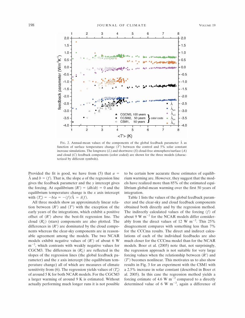
Provided the fit is good, we have from (5) that a �� and b � � f �. That is, the slope a of the regression linegives the feedback parameter and the y intercept givesthe forcing. At equilibrium �R�� dh/dt� � 0 and theequilibrium temperature change is the x axis interceptwith �T�e� � �b/a � �� f �/� � s� f �.

All three models show an approximately linear rela-tion between �R�� and �T�� with the exception of theearly years of the integrations, which exhibit a positiveoffset of �R�� above the best-fit regression line. Thecloud �R�C� (stars) components are also plotted. Thedifferences in �R�� are dominated by the cloud compo-nents whereas the clear-sky components are in reason-able agreement among the models. The two NCARmodels exhibit negative values of �R�� of about 6 Wm�2, which contrasts with weakly negative values forCGCM3. The differences in �R�C� are reflected in theslopes of the regression lines (the global feedback pa-rameter) and the x axis intercept (the equilibrium tem-perature change) all of which are measures of climatesensitivity from (6). The regression yields values of �T�e�of around 5 K for both NCAR models. For the CGCM3a larger warming of around 9 K is estimated. Withoutactually performing much longer runs it is not possible

to be certain how accurate these estimates of equilib-rium warming are. However, they suggest that the mod-els have realized more than 85% of the estimated equi-librium global-mean warming over the first 50 years ofintegration.

Table 1 lists the values of the global feedback param-eter and the clear-sky and cloud feedback componentsobtained both directly and by the regression method.The indirectly calculated values of the forcing � f � ofabout 9 W m�2 for the NCAR models differ consider-ably from the direct values of 12 W m�2. This 25%disagreement compares with something less than 7%for the CCCma results. The direct and indirect calcu-lations of each of the individual feedbacks are alsomuch closer for the CCCma model than for the NCARmodels. Boer et al. (2005) note that, not surprisingly,the regression approach is not suitable for very largeforcing values when the relationship between �R�� and�T�� becomes nonlinear. This motivates us to also showresults in Fig. 3 for an experiment with the CSM1 witha 2.5% increase in solar constant (described in Boer etal. 2005). In this case the regression method yields aforcing estimate of 4.6 W m�2 compared to a directlydetermined value of 6 W m�2, again a difference of

FIG. 2. Annual-mean values of the components of the global feedback parameter � asfunction of surface temperature change �T�� between the control and 5% solar constantincrease simulations. The longwave (L) and shortwave (S) cloud-free atmosphere/surface (A)and cloud (C) feedback components (color coded) are shown for the three models (charac-terized by different symbols).


Fig 2 live 4/C

about 25%. The result is that the indirect method ap-parently underestimates the forcing by about one-quarter for the NCAR models. There is considerablybetter agreement in the two methods for CGCM3.

These results indicate that the Gregory et al. (2004)regression approach may have some practical limitationin its application, at least for some models. It is strikingthat our analysis shows such a large difference in thebehavior among the individual models in this respect.The CCCma model has a radiative imbalance that doesscale reasonably linearly with the realized surfacewarming over the entire experiment. The NCAR mod-els, on the other hand, show a very strong departurefrom this linear relation during the early years of theexperiment. It would be interesting to repeat this analy-sis for other models and see if a similar range of be-havior appears and whether the form of the radiativeimbalance-versus-realized warming relation correlateswith other aspects of model sensitivity.

5. Geographical pattern of the feedback

The geographical pattern of the feedback is ex-pressed as the local contribution �l to the global feed-back parameter such that �� l�. From (1)

�l � �R� � f��T�� g��T�� A� � f � dh��dt��T��.

�9�

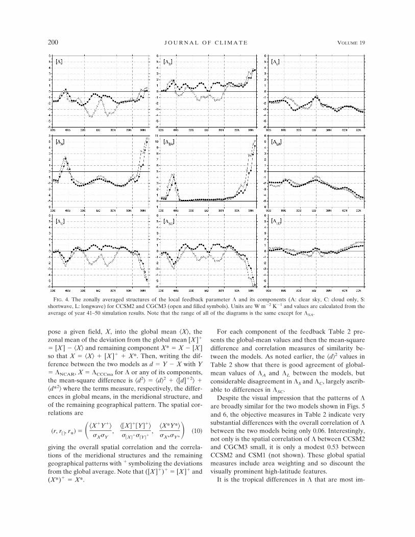
The subscript l is omitted in the following discussion.Here we will present annual-mean values of the feed-back diagnosed from years 41–50 of each of the simu-lations. The zonal-mean values of the feedback, [�],and its components for CCSM2 and CGCM3 are com-pared in Fig. 4. A map of the feedback and componentsfor CCSM2 is shown in Fig. 5 and for CGCM3 in Fig. 6.The CSM1 results (not shown) are reasonably similar tothose from CCSM2.

Figure 4 shows that the difference in the global-meantotal feedback, �� is attributable mainly to differencesin the Tropics and subtropics where the NCAR model’sfeedback is much more negative than that of theCCCma model. The meridional variation of three ofthe four individual components �SA, �LA, and �LC, arequite similar for the two models, but the shortwavecloud feedback �SC is quite different in the two models,particularly in the latitude belt 30°S–30°N.

To provide objective comparisons of the feedbacksbetween the models some simple calculations havebeen performed, starting with the full annual-meanfeedback values depicted in Figs. 5 and 6. We decom-

FIG. 3. The evolution of the global- and annual-mean radiative flux �R�� with temperaturechange �T�� for the three models (color-coded triangles). The cloud �R�C� (stars) componentsare also shown. Open symbols give monthly mean values over the first year of integration. Thedirect estimate of climate forcing from (2) is marked by the heavy black arrow. The CSM1result for a 2.5% increase in solar constant is also shown (green triangles).


Fig 3 live 4/C

pose a given field, X, into the global mean �X�, thezonal mean of the deviation from the global mean [X ]�

� [X ] � �X� and remaining component X* � X � [X ]so that X � �X� � [X ]� � X*. Then, writing the dif-ference between the two models as d � Y � X with Y� �NCAR, X � �CCCma for � or any of its components,the mean-square difference is �d2� � �d�2 � �[d]�2� ��d*2� where the terms measure, respectively, the differ-ences in global means, in the meridional structure, andof the remaining geographical pattern. The spatial cor-relations are

�r, r� �, r*� � ��X�Y��X�Y

,��X��Y��X�

��Y��

,�X*Y*��X*�Y*

� �10�

giving the overall spatial correlation and the correla-tions of the meridional structures and the remaininggeographical patterns with � symbolizing the deviationsfrom the global average. Note that ([X ]�)� � [X ]� and(X*)� � X*.

For each component of the feedback Table 2 pre-sents the global-mean values and then the mean-squaredifference and correlation measures of similarity be-tween the models. As noted earlier, the �d�2 values inTable 2 show that there is good agreement of global-mean values of �A and �L between the models, butconsiderable disagreement in �S and �C, largely ascrib-able to differences in �SC.

Despite the visual impression that the patterns of �are broadly similar for the two models shown in Figs. 5and 6, the objective measures in Table 2 indicate verysubstantial differences with the overall correlation of �between the two models being only 0.06. Interestingly,not only is the spatial correlation of � between CCSM2and CGCM3 small, it is only a modest 0.53 betweenCCSM2 and CSM1 (not shown). These global spatialmeasures include area weighting and so discount thevisually prominent high-latitude features.

It is the tropical differences in � that are most im-

FIG. 4. The zonally averaged structures of the local feedback parameter � and its components (A: clear sky, C: cloud only, S:shortwave, L: longwave) for CCSM2 and CGCM3 (open and filled symbols). Units are W m�2 K�1 and values are calculated from theaverage of year 41–50 simulation results. Note that the range of all of the diagrams is the same except for �SA.


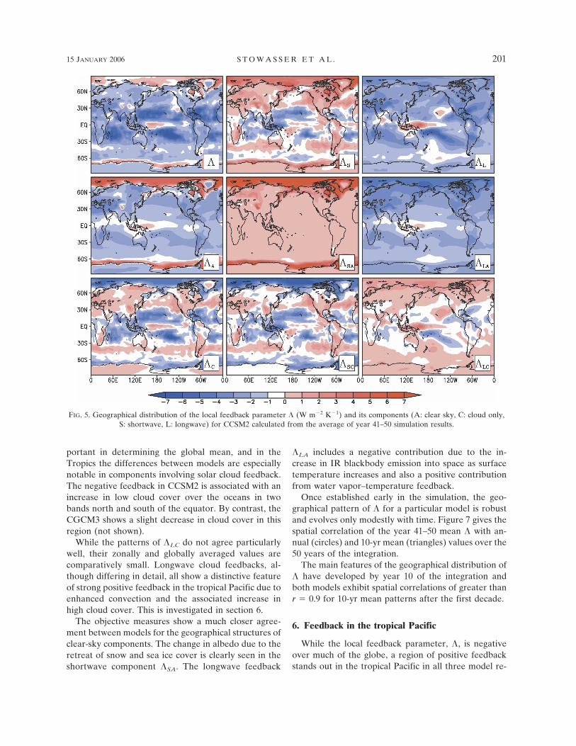
portant in determining the global mean, and in theTropics the differences between models are especiallynotable in components involving solar cloud feedback.The negative feedback in CCSM2 is associated with anincrease in low cloud cover over the oceans in twobands north and south of the equator. By contrast, theCGCM3 shows a slight decrease in cloud cover in thisregion (not shown).

While the patterns of �LC do not agree particularlywell, their zonally and globally averaged values arecomparatively small. Longwave cloud feedbacks, al-though differing in detail, all show a distinctive featureof strong positive feedback in the tropical Pacific due toenhanced convection and the associated increase inhigh cloud cover. This is investigated in section 6.

The objective measures show a much closer agree-ment between models for the geographical structures ofclear-sky components. The change in albedo due to theretreat of snow and sea ice cover is clearly seen in theshortwave component �SA. The longwave feedback

�LA includes a negative contribution due to the in-crease in IR blackbody emission into space as surfacetemperature increases and also a positive contributionfrom water vapor–temperature feedback.

Once established early in the simulation, the geo-graphical pattern of � for a particular model is robustand evolves only modestly with time. Figure 7 gives thespatial correlation of the year 41–50 mean � with an-nual (circles) and 10-yr mean (triangles) values over the50 years of the integration.

The main features of the geographical distribution of� have developed by year 10 of the integration andboth models exhibit spatial correlations of greater thanr � 0.9 for 10-yr mean patterns after the first decade.

6. Feedback in the tropical Pacific

While the local feedback parameter, �, is negativeover much of the globe, a region of positive feedbackstands out in the tropical Pacific in all three model re-

FIG. 5. Geographical distribution of the local feedback parameter � (W m�2 K�1) and its components (A: clear sky, C: cloud only,S: shortwave, L: longwave) for CCSM2 calculated from the average of year 41–50 simulation results.


Fig 5 live 4/C

sults, although its location and extent differs in each.This feature is largely, but not entirely, attributable tothe longwave cloud feedback �LC (see Figs. 5 and 6)and is connected to a permanent El Niño–like warming

in the models as the global-mean temperature rises.Boer et al. (2004) argue that this region of positivefeedback also operates to produce the La Niña–likepattern that is seen in simulations of the Last Glacial

FIG. 6. As in Fig. 5 but for the CGCM3 results.

TABLE 2. The global-mean values of the feedback parameter � and its components for the averages of years 41–50 for the CCSM2and CGCM3 (W m�2 K�1). Also given are the mean-square differences and spatial correlations between CCSM2 and CGCM3 resultsin global means, meridional structure, and of the remaining geographical pattern.

� �S �L �A �C �SA �SC �LA �LC

Global meanCCSM2 �2.30 �0.10 �2.20 �1.36 �0.94 0.76 �0.86 �2.12 �0.08CGCM3 �1.29 1.01 �2.30 �1.58 0.29 0.68 0.33 �2.26 �0.04

Mean-square diff�d�2 1.03 1.24 0.01 0.05 1.53 0.01 1.42 0.02 0.00�[d]�2� 1.81 1.15 0.27 0.23 1.38 0.36 0.77 0.11 0.21�d*2� 2.12 2.15 1.65 0.97 1.65 0.94 2.10 0.29 0.79

Spatial correlationsr 0.06 0.24 0.35 0.74 0.22 0.81 0.38 0.75 0.27r[ ]� �0.08 0.26 0.68 0.92 0.13 0.95 0.60 0.92 0.53r* 0.15 0.24 0.22 0.54 0.29 0.61 0.22 0.57 0.17


Fig 6 live 4/C

Maximum (LGM) with CGCM2 and some other mod-els (in response to a negative climate forcing in thiscase). In addition to the obvious regional implicationsfor an El Niño–like response in the Pacific (e.g., Meehl1996), there is the possibility that the mechanism lead-ing to the tropical Pacific positive feedback patch actsto significantly affect the global feedback and increaseclimate sensitivity. Alternatively, this mechanism mayonly produce a modification of the feedback patternwithout significantly affecting the global average.

The El Niño–like nature of the warming pattern is aconsequence of basin-scale equatorial ocean dynamicsaccording to Boer and Yu (2003c) who show, in anearlier version (CGCM1) of the CCCma coupledmodel, that both the region of positive feedback in thetropical Pacific and the El Niño–like temperature re-sponse are absent in a simulation with a mixed layer orthermodynamic-only ocean component. Meehl et al.(2000) examine the surface temperature response inglobal warming simulations with atmospheric modelscoupled to a mixed layer ocean to suppress the effectsof ocean dynamics; their results suggest that the devel-opment of the permanent El Niño–like warming in thetropical Pacific might enhance the global-mean surfacewarming by 5% and that the El Niño–like warmingresponse in the model was attributed to cloud feed-backs interacting with the radiative forcing. Of course,observations of the interannual variability in the realworld show that globally averaged surface tempera-tures are anomalously warm during an El Niño event(e.g., Nicholls 1992), but the two situations are not nec-essarily parallel. In particular, Yu and Boer (2002)

show that the mean El Niño–like warming pattern inCGCM1 is sustained by oceanic heat transports into theregion, while observational results suggest that oceanicheat transports are away from the region in the usualtransient El Niño event.

The feedback parameter and the change in surfacetemperature in the tropical Pacific region are shown inFig. 8 for all three of the present model warming ex-periments.

The tropical Pacific region of positive � is associatedwith an El Niño–like SST warming pattern in the cen-tral Pacific for CSM1, in the western Pacific forCCSM2, and in the central eastern Pacific for CGCM3.The region of positive feedback is surrounded by com-paratively strong negative feedback in the NCAR mod-

FIG. 7. The evolution of the spatial pattern of � as measured bythe spatial correlation with the year 41–50 mean pattern. Filledand open circles are for annual-mean values, and triangles are for10-yr means for CCSM2 and CGCM3, respectively.

FIG. 8. Feedback parameter � (shaded in W m�2 K�1) and thechange in surface temperatures (contours in K) calculated fromthe average of years 41–50 of (a) CSM1, (b) CCSM2, and (c)CGCM3 simulation results.


Fig 8 live 4/C

els, and this serves to localize the temperature maxi-mum in that region. By contrast, the CGCM3 feedbackpattern is broader, less localized, and less congruent tothe temperature pattern. In all of the models the largestlongwave cloud feedback is associated with the greatestchanges in surface temperature. Most previous globalwarming simulations have exhibited a mean El Niño–like warming (e.g., Meehl and Washington 1996; Tim-mermann et al. 1999; Boer et al. 2000; Cai and Whetton2000), but there are exceptions with some models simu-lating a bland tropical SST change pattern (Meehl et al.2000) or even a La Niña–like pattern (Noda et al. 1999).

Rewriting (1) and then assuming that the change inoceanic heat storage in the Tropics is comparativelysmall, we obtain

R� � R�A � C� � �A� � �l�T�� f. �11�

This highlights the connection to the change in energyconvergence, A�, in the atmosphere and ocean. Here R�� R�A � C�, where R�A is the cloud-free change in ra-diative flux and C� is the change in cloud radiative forc-ing.

Atmospheric energy transport is closely connected tothe the divergent flow in the Tropics (Boer and Sargent1985; Trenberth et al. 2000). Figure 9 plots the controlrun 200-hPa divergent wind vectors and associated ve-locity potential for CCSM2 and CGCM3 together with

the change in these quantities for the 5% solar constantincrease experiment. The regions of divergence in thecontrol simulations are associated with regions of warmsea surface temperatures and high latent heat releaseand the flux of energy is toward cold continental andoceanic regions. These patterns are clearly related tothe upper-tropospheric components of the Hadley–Walker circulation. The Walker circulation in the equa-torial east–west plane over the Pacific is represented bythe streamfunction associated with the divergent east–west wind component uD for the equatorial band 5°N–5°S calculated as �(p, �) � �p

0 uD dp/g. This is plottedfor the control runs for CCSM2 and CGCM3 in the toppanels of Fig. 10. The bottom panels show the changesin � in the perturbed experiments for both models.

Large centers of upper-tropospheric divergence (andlower-tropospheric convergence) in the central andwestern equatorial Pacific warm pool region are appar-ent in the control runs of both models. The equatorialeastern Pacific cold tongue is associated with upper-tropospheric convergence. The associated Walker cir-culation is distinctly stronger in CGCM3 than inCCSM2.

In the perturbed runs the overall strength of theWalker circulation is reduced in CGCM3. In theCCSM2, by contrast, the upper-tropospheric diver-gence strengthens in the western Pacific warm pool and

FIG. 9. Divergent wind vectors and the corresponding velocity potential for the CCSM2 and CGCM3 models at the 200-hPa level(mean of years 41–50). (top) Control-run values and (bottom) the changes in the 5% solar constant increase simulation. Units are 103

kg m�1 s�1 and 108 kg s�1, respectively.


the Walker circulation is actually slightly enhanced,leading to an increase in convection and high cloudcover in this region. Both models simulate an increasedconvergence over the Indian Ocean and SoutheastAsia, but this feature is again more pronounced inCGCM3.

Much of the geographical structure of the feedbackin the tropical Pacific is associated with the longwavecloud component, �LC, which is strongly positive in thewestern Pacific in the CCSM2 simulation (see Fig. 5).To investigate the importance of air–sea interactions indetermining the �LC distribution, a separate integra-tion with prescribed SSTs was performed. In particular,the CCSM2 model was run with exactly the same 5%increase solar constant but with prescribed SSTs andsea ice concentrations. These were taken from theoriginal 5% perturbation simulation everywhere exceptin a region of the western Pacific bounded by 8°S–8°N,140°–220°E. Here the SST was prescribed as the controlrun value plus a warming field based on the original 5%perturbation model results, but smoothed in this regionto suppress zonal gradients in the warming, while re-taining the average surface temperature increase overthe region.

The longwave cloud feedback parameter �LC and the

temperature change for the two cases are shown in Fig.11. The smoothing of the temperature change patternhas a strong influence on �LC; the strong positive cen-ter in the western Pacific wanes and even becomesslightly negative, consistent with of the results of Boerand Yu (2003c) for a mixed layer ocean. Here, the sig-nificant effects are restricted to the region where thesmoothing is applied. The signal is not so striking in �itself since �SC increases and partially counteracts thechange in �LC (not shown).

From (11) we may approximate the change betweenthe two cases as �R� � ��A� � �C� � ��T�� so that

�� A��T�� C��T�� 12�

and the change in feedback is approximately connectedto a change in transport and cloud forcing.

Despite the difference in � in the tropical Pacific inthese two experiments the global mean feedback, andhence the climate sensitivity, changes only slightly,from �2.3 W m�2 K�1 in the coupled model case to�2.2 W m�2 K�1 with prescribed smoothed SSTs. Thissuggests that in the full coupled model the positivefeedback associated with the SST maximum is morethan balanced by enhanced negative feedback else-where. The implication is that the tropical Pacific maxi-

FIG. 10. The mean streamfunction associated with the divergent east–west mass circulation for the years 41–50 ofthe control runs of CCSM2 and CGCM3. (bottom) The change in the 5% solar constant increase run is shown. Units are109 kg s�1.


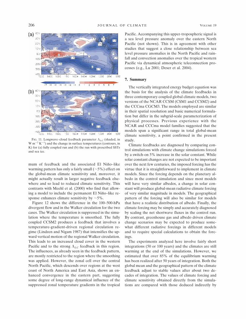
mum of feedback and the associated El Niño–likewarming pattern has only a fairly small (�5%) effect onthe global-mean climate sensitivity and, moreover, itmight actually result in larger negative feedback else-where and so lead to reduced climate sensitivity. Thiscontrasts with Meehl et al. (2000) who find that allow-ing a model to include the permanent El Niño–like re-sponse enhances climate sensitivity by �5%.

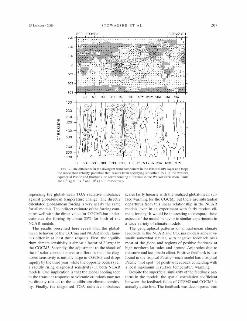
Figure 12 shows the difference in the 100–500-hPadivergent flow and in the Walker circulation for the twocases. The Walker circulation is suppressed in the simu-lation where the temperature is smoothed. The fullycoupled CCSM2 produces a feedback that involves atemperature-gradient-driven regional circulation re-gime (Lindzen and Nigam 1987) that intensifies the up-ward vertical motion of the regional Walker circulation.This leads to an increased cloud cover in the westernPacific and to the strong �LC feedback in this region.The influences, as already seen in the feedback pattern,are mostly restricted to the region where the smoothingwas applied. However, the zonal cell over the centralNorth Pacific, which descends over regions at the westcoast of North America and East Asia, shows an en-hanced convergence in the eastern part, suggestingsome degree of long-range dynamical influence of thesuppressed zonal temperature gradients in the tropical

Pacific. Accompanying this upper-tropospheric signal isa sea level pressure anomaly over the eastern NorthPacific (not shown). This is in agreement with otherstudies that suggest a close relationship between sealevel pressure anomalies in the North Pacific and rain-fall and convection anomalies over the tropical westernPacific via dynamical atmospheric teleconnection pro-cesses (e.g., Lu 2001; Deser et al. 2004).

7. Summary

The vertically integrated energy budget equation wasthe basis for the analysis of the climate feedbacks inthree contemporary coupled global climate models, twoversions of the NCAR CCSM (CSM1 and CCSM2) andthe CCCma CGCM3. The models employed are similarin their spatial resolution and basic numerical formula-tion but differ in the subgrid-scale parameterization ofphysical processes. Previous experience with theNCAR and CCCma model families suggested that themodels span a significant range in total global-meanclimate sensitivity, a point confirmed in the presentstudy.

Climate feedbacks are diagnosed by comparing con-trol simulations with climate change simulations forcedby a switch-on 5% increase in the solar constant. Whilesolar constant changes are not expected to be importantover the next few centuries, the imposed forcing has thevirtue that it is straightforward to implement in climatemodels. Since the forcing depends on the planetary al-bedo in the control simulation and since most modelswill have very similar albedos, a change in solar con-stant will produce global-mean radiative climate forcingof very similar magnitude in models. The geographicalpattern of the forcing will also be similar for modelsthat have a realistic distribution of albedo. Finally, theclimate forcing may be simply and accurately diagnosedby scaling the net shortwave fluxes in the control run.By contrast, greenhouse gas and albedo driven climatechange scenarios may be expected to produce some-what different radiative forcings in different modelsand to require special calculations to obtain the forc-ings.

The experiments analyzed here involve fairly shortintegrations (50 or 100 years) and the climates are stillwarming at the end of the simulations. However, weestimated that over 85% of the equilibrium warminghas been realized after 50 years of integration. Both theglobal mean and the geographical pattern of the climatefeedback adjust to stable values after about two de-cades of integration. The values of climate forcing andclimate sensitivity obtained directly from the simula-tions are compared with those deduced indirectly by

FIG. 11. Longwave–cloud feedback parameter �LC (shaded, inW m�2 K�1) and the change in surface temperatures (contours, inK) for (a) fully coupled run and (b) the run with prescribed SSTsand sea ice.


Fig 11 live 4/C

regressing the global-mean TOA radiative imbalanceagainst global-mean temperature change. The directlycalculated global-mean forcing is very nearly the samefor all models. The indirect estimate of the forcing com-pares well with the direct value for CGCM3 but under-estimates the forcing by about 25% for both of theNCAR models.

The results presented here reveal that the global-mean behavior of the CCCma and NCAR model fami-lies differ in at least three respects. First, the equilib-rium climate sensitivity is almost a factor of 2 larger inthe CGCM3. Secondly, the adjustment to the shock ofthe of solar constant increase differs in that the diag-nosed sensitivity is initially large in CGCM3 and dropsrapidly by the third year, while the opposite occurs (i.e.,a rapidly rising diagnosed sensitivity) in both NCARmodels. One implication is that the global cooling seenin the transient response to volcanic eruptions may notbe directly related to the equilibrium climate sensitiv-ity. Finally, the diagnosed TOA radiative imbalance

scales fairly linearly with the realized global-mean sur-face warming for the CGCM3 but there are substantialdepartures from this linear relationship in the NCARmodels, even in an experiment with fairly modest cli-mate forcing. It would be interesting to compare theseaspects of the model behavior in similar experiments ina wide variety of climate models.

The geographical patterns of annual-mean climatefeedback in the NCAR and CCCma models appear vi-sually somewhat similar, with negative feedback overmost of the globe and regions of positive feedback athigh northern latitudes and around Antarctica due tothe snow and ice albedo effect. Positive feedback is alsofound in the tropical Pacific—each model has a tropicalPacific “hot spot” of positive feedback coinciding witha local maximum in surface temperature warming.

Despite the superficial similarity of the feedback pat-terns in the models, the spatial correlation coefficientbetween the feedback fields of CCSM2 and CGCM3 isactually quite low. The feedback was decomposed into

FIG. 12. The difference in the divergent wind component in the 100–500-hPa layer and (top)the associated velocity potential that results from specifying smoothed SST in the westernequatorial Pacific and (bottom) the corresponding difference in the Walker circulation. Unitsare 103 kg m�1 s�1 and 108 kg s�1, respectively.


shortwave and longwave/clear-sky (atmosphere/sur-face) and cloud components. The mean-square differ-ences and spatial correlations between the models werecomputed for each component. The clear-sky compo-nents have reasonably large correlation coefficientsand, indeed, the clear-sky feedback maps look quitesimilar for the CCCma and NCAR models. The lowspatial correlation and large mean-square differencebetween the total feedback patterns in the models islargely a consequence of a marked difference in theshortwave cloud feedback component in the Tropicsand subtropics. The NCAR models have strong nega-tive shortwave cloud feedback over most of the bandbetween 30°S and 30°N due to an increase in low-cloudcover over the oceans in bands north and south of theequator. This contrasts with a slight decrease in cloudcover and a weak positive shortwave cloud feedback inCGCM3. The result is that the NCAR models exhibitstronger negative global-mean feedback than doesCGCM3, resulting in a considerably lower climate sen-sitivity.

All three models display a local maximum in surfacewarming and a region of positive total feedback in thetropical Pacific region. However, the models differ inthe zonal structure of the simulated surface warming,with results ranging from a mean El Niño–like warmingin the eastern Pacific in the CGCM3 to a peak warmingin the far western Pacific in the CCSM2 model. A sepa-rate global warming simulation for the CCSM2 was per-formed in which the zonal gradients in the temperatureresponse pattern in the tropical Pacific were sup-pressed. In this simulation the region of positive feed-back in the tropical Pacific is absent, but the global-mean negative feedback is about 5% greater than thatin standard experiment. The implication is that thecoupled atmosphere–ocean processes that lead to thetropical region of positive feedback and the associatedSST maximum only modestly influence the global-mean climate sensitivity, and might actually act toslightly reduce the global sensitivity.

Acknowledgments. The authors acknowledge the as-sistance of Ping Liu and Weijun Zhu with the NCARmodel runs. This research was supported by the JapanAgency for Marine-Earth Science and Technology(JAMSTEC) through its sponsorship of the Interna-tional Pacific Research Center.

REFERENCES

Boer, G. J., and N. Sargent, 1985: Vertically integrated budgets ofmass and energy for the globe. J. Atmos. Sci., 42, 1592–1613.

——, and B. Yu, 2003a: Climate sensitivity and climate state.Climate Dyn., 21, 167–176.

——, and ——, 2003b: Climate sensitivity and response. ClimateDyn., 20, 415–429.

——, and ——, 2003c: Dynamical aspects of climate sensitivity.Geophys. Res. Lett., 30, 1135, doi:10.1029/2002GL016549.

——, G. Flato, and D. Ramsden, 2000: A transient climate changesimulation with greenhouse gas and aerosol forcing: Pro-jected climate for the 21st century. Climate Dyn., 16, 427–450.

——, B. Yu, S. J. Kim, and G. Flato, 2004: Is there observationalsupport for an El Niño-like pattern of future global warming?Geophys. Res. Lett., 31, L06201, doi:10.1029/2003GL018722.

——, K. Hamilton, and W. Zhu, 2005: Climate sensitivity andclimate change under strong forcing. Climate Dyn., 24,doi:10.1007/s00382-004-0500-3.

Boville, B. A., and P. R. Gent, 1998: The NCAR climate systemmodel, version one. J. Climate, 11, 1115–1130.

——, J. T. Kiehl, P. J. Rasch, and F. O. Bryan, 2001: Improve-ments to the NCAR CSM-1 for transient climate simulations.J. Climate, 14, 164–179.

Cai, W., and P. Whetton, 2000: Evidence for a time-varying pat-tern of greenhouse warming in the Pacific Ocean. Geophys.Res. Lett., 27, 2577–2580.

Cess, R. D., and Coauthors, 1990: Intercomparison and interpre-tation of climate feedback processes in 19 atmospheric gen-eral circulation models. J. Geophys. Res., 95, 16 601–16 615.

Collins, W. D., 2001: Parameterization of generalized cloud over-lap for radiative calculations in general circulation models. J.Atmos. Sci., 58, 3224–3242.

——, J. K. Hackney, and D. P. Edwards, 2002: An updated pa-rameterization for infrared emission and absorption by watervapor in the National Center for Atmospheric Research com-munity atmosphere model. J. Geophys. Res., 107, 4664,doi:10.1029/2001JD001365.

Colman, R., 2003: A comparison of climate feedback in generalcirculation models. Climate Dyn., 20, 865–873.

Dai, A., T. M. L. Wigley, B. A. Boville, J. T. Kiehl, and L. E. Buja,2001: Climates of the twentieth and twenty-first centuriessimulated by the NCAR Climate System Model. J. Climate,14, 485–519.

Deser, C., A. S. Phillips, and J. W. Hurrell, 2004: Pacific interdec-adal climate variability: Linkages between the Tropics andthe North Pacific during boreal winter since 1900. J. Climate,17, 3109–3124.

Flato, G., G. J. Boer, W. Lee, N. McFarlane, D. Ramsden, and A.Weaver, 2000: The CCCma global coupled model and itsclimate. Climate Dyn., 16, 451–467.

Gregory, J. M., and Coauthors, 2004: A new method for diagnos-ing radiative forcing and climate sensitivity. Geophys. Res.Lett., 31, L03205, doi:10.1029/2003GL018747.

Hansen, J., M. Sato, and R. Reudy, 1997: Radiative forcing andclimate response. J. Geophys. Res., 102, 6831–6864.

Houghton, J. T., Y. Ding, D. J. Griggs, M. Noguer, P. J. van derLinden, X. Dai, K. Maskell, and C. A. Johnson, Eds., 2001:Climate Change 2001: The Scientific Basis. Cambridge Uni-versity Press, 881 pp.

Kiehl, J. T., and P. R. Gent, 2004: The Community Climate Sys-tem model, version 2. J. Climate, 17, 3666–3682.

——, J. J. Hack, G. B. Bonan, B. B. Boville, D. L. Williamson, andP. J. Rasch, 1998: The National Center for Atmospheric Re-search Community Climate Model: CCM3. J. Climate, 11,1131–1150.

Lacis, A. A., and J. Hansen, 1974: A parameterization for theabsorption of solar radiation in the earth’s atmosphere. J.Atmos. Sci., 31, 118–133.


Lindzen, R. S., and S. Nigam, 1987: On the role of sea surfacetemperature gradients in forcing low level winds and conver-gence in the tropics. J. Atmos. Sci., 44, 2418–2436.

Lu, R., 2001: Interannual variability of the summertime NorthPacific subtropical high and its relation to atmospheric con-vection over the warm pool. J. Meteor. Soc. Japan, 79, 771–783.

Meehl, G. A., 1996: Vulnerability of fresh water resources to cli-mate change in the tropical Pacific region. J. Water. Air SoilPollut., 92, 203–213.

——, and W. M. Washington, 1996: El Niño-like climate change ina model with increased atmospheric CO2 concentration. Na-ture, 382, 56–60.

——, W. D. Collins, B. A. Boville, J. T. Kiehl, T. M. L. Wigley,and J. M. Arblaster, 2000: Response of the NCAR climatesystem model to increased CO2 and the role of physical pro-cesses. J. Climate, 13, 1879–1898.

——, W. M. Washington, C. M. Ammann, J. M. Arblaster, T. M.L. Wigley, and C. Tebaldi, 2004: Combination of natural andanthropogenic forcings in twentieth-century climate. J. Cli-mate, 17, 3721–3727.

Nicholls, N. G., 1992: Observed climate variability and change.Climate Change 1992: The Supplementary Report to the IPCCScientific Assessment, J. T. Houghton, B. A. Callander, andS. K. Varney, Eds., Cambridge University Press, 133–192.

Noda, A., K. Yamaguchi, S. Yamaki, and S. Yukimoto, 1999:Relationship between natural variability and CO2 inducedwarming pattern: MRI AOGCM experiment. Preprints, 10thSymp. on Global Change Studies, Dallas, TX, Amer. Meteor.Soc., 359–364.

Rasch, P. J., and J. E. Kristjánsson, 1998: A comparison of theCCM3 model climate using diagnosed and predicted conden-sate parameterizations. J. Climate, 11, 1587–1614.

Scinocca, J. F., and N. A. McFarlane, 2004: The variability ofmodeled tropical precipitation. J. Atmos. Sci., 61, 1993–2015.

Senior, C. A., and J. F. B. Mitchell, 2000: The time dependence ofclimate sensitivity. Geophys. Res. Lett., 27, 2685–2688.

Slingo, J. M., 1987: The development and verification of a cloudprediction scheme for the ECMWF model. Quart. J. Roy.Meteor. Soc., 113, 899–927.

Timmermann, A., M. Latif, A. Bacher, J. Oberhuber, and E.Roeckner, 1999: Increased El Niño frequency in a climatemodel forced by future greenhouse warming. Nature, 398,694–697.

Trenberth, K. E., D. P. Stepaniak, and J. M. Caron, 2000: Theglobal monsoon as seen through the divergent atmosphericcirculation. J. Climate, 13, 3969–3993.

Watterson, I. G., 2000: Interpretation of simulated global warm-ing using a simple model. J. Climate, 13, 202–215.

——, M. R. Dix, and R. A. Colman, 1999: A comparison ofpresent and doubled CO2 climates and feedbacks simulatedby three GCMs. J. Geophys. Res., 104, 1943–1956.

Yu, B., and G. J. Boer, 2002: The roles of radiation and dynamicalprocesses in the El Niño–like response to global warming.Climate Dyn., 19, 539–553.

Zhang, M. H., W. Y. Lin, C. Bretherton, J. J. Hack, and P. J.Rasch, 2003: A modified formulation of fractional stratiformcondensation rate in the NCAR Community AtmosphericModel (CAM2). J. Geophys. Res., 108, 4035, doi:10.1029/2002JD002523.


Local and Global Climate Feedbacks in Models with Differing Climate Sensitivities

Documents

Transcript of Local and Global Climate Feedbacks in Models with Differing Climate Sensitivities