1 23

Climate DynamicsObservational, Theoretical andComputational Research on the ClimateSystem ISSN 0930-7575Volume 39Combined 3-4 Clim Dyn (2012) 39:575-588DOI 10.1007/s00382-011-1104-3

Uncertainty in the ocean–atmospherefeedbacks associated with ENSO in thereanalysis products

Arun Kumar & Zeng-Zhen Hu

1 23

Your article is protected by copyright and

all rights are held exclusively by Springer-

Verlag (outside the USA). This e-offprint is

for personal use only and shall not be self-

archived in electronic repositories. If you

wish to self-archive your work, please use the

accepted author’s version for posting to your

own website or your institution’s repository.

You may further deposit the accepted author’s

version on a funder’s repository at a funder’s

request, provided it is not made publicly

available until 12 months after publication.

Uncertainty in the ocean–atmosphere feedbacks associatedwith ENSO in the reanalysis products

Arun Kumar • Zeng-Zhen Hu

Received: 29 March 2011 / Accepted: 18 May 2011 / Published online: 4 June 2011

� Springer-Verlag (outside the USA) 2011

Abstract The evolution of El Nino-Southern Oscillation

(ENSO) variability can be characterized by various ocean–

atmosphere feedbacks, for example, the influence of ENSO

related sea surface temperature (SST) variability on the

low-level wind and surface heat fluxes in the equatorial

tropical Pacific, which in turn affects the evolution of the

SST. An analysis of these feedbacks requires physically

consistent observational data sets. Availability of various

reanalysis data sets produced during the last 15 years

provides such an opportunity. A consolidated estimate of

ocean surface fluxes based on multiple reanalyses also

helps understand biases in ENSO predictions and simula-

tions from climate models. In this paper, the intensity and

the spatial structure of ocean–atmosphere feedback terms

(precipitation, surface wind stress, and ocean surface heat

flux) associated with ENSO are evaluated for six different

reanalysis products. The analysis provides an estimate for

the feedback terms that could be used for model validation

studies. The analysis includes the robustness of the esti-

mate across different reanalyses. Results show that one of

the ‘‘coupled’’ reanalysis among the six investigated is

closer to the ensemble mean of the results, suggesting that

the coupled data assimilation may have the potential to

better capture the overall atmosphere–ocean feedback

processes associated with ENSO than the uncoupled ones.

Keywords Reanalysis products � ENSO feedback �Dynamical and thermodynamical processes � Uncertainty �Multi-reanalysis ensemble � Coupled and uncoupled

reanalyses

1 Introduction

El Nino-Southern Oscillation (ENSO) is the most dominant

mode of interannual variability in the tropical climate

system, and is associated with the coupled air–sea inter-

actions in the equatorial tropical Pacific. Sea surface tem-

perature (SST) variability associated with ENSO has global

atmospheric and oceanic climate influence, and is the basic

premise for skillful seasonal climate prediction efforts

(Kumar et al. 2005; National Research Council 2010). As a

consequence, improving ENSO prediction has been a

major effort at many prediction centers over the world.

Given the societal impacts of ENSO, an understanding

of its characteristics and variability under a changing

climate is also an intense area of research (Guilyardi et al.

2009a, b).

Improving ENSO prediction relies on the understanding

of the features of ENSO variability, improvements in

ENSO prediction tools, and availability of physically

consistent observational data sets for validation. A tool

for generating ENSO predictions is the coupled ocean–

atmosphere general circulation models (CGCMs) that are

initialized with the observed state of the ocean and atmo-

sphere, and are integrated forward in time. To advance the

current level of ENSO prediction skill, and to build con-

fidence in changes in ENSO characteristics under an

evolving climate, efforts are continually under way to

improve CGCMs that are used for ENSO prediction and

projections. Such efforts require an assessment of coupled

model simulations, and their validation against the

observed characteristics of ENSO. A key factor in vali-

dating coupled model predictions and simulations is the

strength and the spatial structure of the coupled air-sea

feedbacks that are important in determining ENSO feature.

Such feedbacks include the interaction between the ENSO

A. Kumar (&) � Z.-Z. Hu

Climate Prediction Center, NCEP/NWS/NOAA, 5200 Auth

Road (Suite 605), Camp Springs, MD 20746, USA

e-mail: Arun.Kumar@NOAA.GOV

123

Clim Dyn (2012) 39:575–588

DOI 10.1007/s00382-011-1104-3

Author's personal copy

SST, precipitation, surface wind stress, as well as various

surface heat fluxes, e.g. latent heat, and surface shortwave

radiation (e.g. Bjerknes 1969; Philander 1990; Barnett et al.

1991; Neelin et al. 1998, Wang and Picaut 2004; Sun et al.

2006, 2009; Lloyd et al. 2009, 2011).

Over the past decade, several global reanalysis efforts

have generated a three dimensional rendition of the evo-

lution of the climate system. These reanalyses have been

treated as ‘‘observations’’ and have been used to validate

the basic features of coupled air–sea feedback related to

ENSO (Okumura and Deser 2010; Xue et al. 2011). These

physically coherent data sets have also been used as initial

conditions for seasonal climate predictions and for gen-

erating hindcasts, as well as validating the fidelity of long-

term climate change projections (IPCC 2007; National

Research Council 2010). Reanalysis products, however,

are themselves dependent on models and data assimilation

systems. As a consequence, in data sparse regions, such as

the southern ocean, reanalysis products may be entirely an

artifact of the model solution, and could be influenced by

model biases. Therefore, before the reanalysis products

can be used as a basis for validating the air-sea feedbacks

in coupled models, it is important to assess the reliability

of these so-called ‘‘observations’’ and to quantify uncer-

tainty between them. Such an analysis is the focus of this

paper.

In this work, we focus on the uncertainty of the ocean–

atmosphere feedbacks associated with ENSO by examining

ocean surface wind stress, precipitation, and various com-

ponents of ocean surface heat flux in the different reanal-

ysis products, which are dominant in governing the ENSO

evolution in observations and in present-day coupled

models (Schneider 2002; Guilyardi et al. 2004; Kim et al.

2008; references therein). The thermocline, advection, and

Ekman feedbacks which also determine the ENSO evolu-

tion are not examined. The paper is organized as follows:

in Sect. 2 the various observational and reanalysis prod-

ucts, and the analysis procedures used in this paper are

described. A comparison of air-sea feedback terms related

to ENSO between various reanalyses is presented in Sect.

3, followed by a summary and discussion in Sect. 4.

2 Data and analysis procedure

In this study, six different reanalysis products that have

been generated over the last *15 year period are analyzed.

In the chronological order of their availability, these

reanalysis products are: NCEP/NCAR reanalysis (R1;

Kalnay et al. 1996); NCEP-DOE reanalysis (R2; Kanamitsu

et al. 2002; ERA-40 (ERA40; Uppala et al. 2005); JRA-25

(JRA; Onogi et al. 2007); CFSR (Saha et al. 2010); and

MERRA (Rienecker et al. 2011). Data from all these

reanalyses are available for 1979–2009 except for the

ERA40 that only extends to 2001. It should be pointed out

that except CFSR, all these reanalysis products are gener-

ated using atmosphere general circulation models (AG-

CMs) forced by observed SST and with the assimilation of

various observational data. On the other hand, the CFSR is a

partially coupled ocean–atmosphere reanalysis system

(Saha et al. 2010).

The observed interannual ENSO variability is defined

based on the analyzed monthly mean SST data, which is

version 3b of the extended reconstruction of the SST

analyses (ERSSTv3) on a 2 9 2 grid during the period

January 1979–December 2009 (Smith et al. 2008). We also

use the Monthly Climate Prediction Center (CPC) Merged

Analysis of Precipitation (CMAP) on a 2.5 9 2.5 grid from

Jan. 1979–Dec. 2009 (Xie and Arkin 1997). The observed

estimate of latent heat flux over the ocean surface from Jan.

1979-Dec. 2008 is from the objectively analyzed air-sea

flux (OAFlux) (Yu and Weller 2007) and net shortwave

(SW) radiation flux over the ocean surface is from the

International Satellite Cloud Climatology Project (ISCCP,

Zhang et al. 2004).

ENSO evolution involves dynamical and thermody-

namical feedback processes (Bjerknes 1969; Philander

1990; Barnett et al. 1991; Neelin et al. 1998; Wang and

Picaut 2004; Sun et al. 2006, 2009; Lloyd et al. 2009,

2011). Of the important ocean–atmosphere feedback terms

related to ENSO variability are the variations in surface

winds (or the surface wind stress) and surface heat fluxes.

The intensity and spatial pattern of these feedbacks par-

tially depend on the precipitation response to variations in

SSTs. Since precipitation is not an assimilated variable

during the assimilation, it is likely that precipitation

response in various reanalyses may depend on the char-

acteristics of the assimilation system, ingested observa-

tional data, and the model, particularly the atmospheric

component.

In this work, ocean–atmosphere feedbacks associated

with ENSO in various reanalyses are quantified based on

the monthly means of surface wind stress, different heat

(latent, sensible, shortwave, long-wave) flux terms, and

precipitation. The analysis of monthly means, by averaging

the high-frequency atmospheric variability that may be

independent of ENSO, highlights the coupled ocean–

atmosphere interaction related to ENSO. All monthly

anomalies are computed by subtracting the climatology for

each month constructed by averaging over the respective

data periods.

A common way to identify ENSO variability (and

events) is the Nino 3.4 SST index (Barnston et al. 1997).

Using this index as a representation of ENSO variability, a

simple approach of linear regression of different variables

onto the Nino3.4 index for all months is used to quantify

576 A. Kumar, Z.-Z. Hu: Uncertainty in the ocean–atmosphere feedbacks

123

Author's personal copy

the ocean–atmosphere coupling associated with ENSO

variability. The Nino3.4 index is computed using the

ERSSTv3 SST, and although various reanalyses have uti-

lized different SST analyses, the differences in the inter-

annual variability of the Nino3.4 SSTA used in reanalyses

and ERSSTv3 are minor (not shown). Also, general pat-

terns following regressions do not depend on the index

used to represent ENSO.

3 Results

3.1 Dynamical feedbacks

Shown in Fig. 1 is the regression pattern of the ERSSTv3

SST anomaly (SSTA) onto the Nino3.4 index. The spatial

pattern of SSTA regression has the typical ENSO pattern

with warm SSTAs stretching from the west coast of South

America to about the dateline, with the maximum anomaly

straddling the equator (Rasmusson and Carpenter 1982).

The equatorial SSTAs in the Pacific are flanked by a

horseshoe pattern of cold SSTAs in the northern and

southern hemisphere.

Warm SSTAs associated with the positive phase of the

Nino3.4 index result in an eastward shift in the tropical

convection as evident in Fig. 2, where regression of

reanalysis derived precipitation and surface wind stress

anomalies with the Nino3.4 index is shown. All reanalyses

have positive regressions of rainfall anomalies in the

tropical central and eastern Pacific, however, the intensity

and spatial structure have large differences across different

reanalyses. R2 and ERA40 have the largest amplitude for

the precipitation response while R1 has the smallest. Pre-

cipitation responses in MERRA, CFSR, and JRA share

similar amplitude and spatial structure with a comma

shaped pattern extending from the Southern to the Northern

Hemisphere.

Compared with the climatological distribution pattern of

precipitation (shading in Fig. 5), we note that the precipi-

tation regression pattern associated with ENSO (shading in

Fig. 2) represents a northeastward shift of the South Pacific

Convergence Zone (SPCZ) below the equator and

strengthening of the Intertropical Convergence Zone

(ITCZ) above the equator. Both R1 and R2 (Fig. 2a, b),

however, have a more equatorially symmetric precipitation

response pattern, while ERA40 (Fig. 2e) has a hint of a

comma shaped pattern. Differences in precipitation

response to SSTs are likely due to differences in the data

assimilation procedures, and differences in the parameteri-

zation schemes that are part of the AGCM component of the

assimilation system. It is well known that small changes in

adjustable parameters that are part of various parameteri-

zation schemes can lead to a large sensitivity in precipita-

tion to interannual variations in SSTs (Ji et al. 1994).

Precipitation regression for the reanalyses can also be

compared with that for the observation-based estimate of

Fig. 1 Regression of ERSSTv3

SST anomalies onto the Nino3.4

index computed used ERSSTv3

SSTA. Contour interval is 0.2

of per unit standard deviation

(STDV) of the Nino3.4 index

A. Kumar, Z.-Z. Hu: Uncertainty in the ocean–atmosphere feedbacks 577

123

Author's personal copy

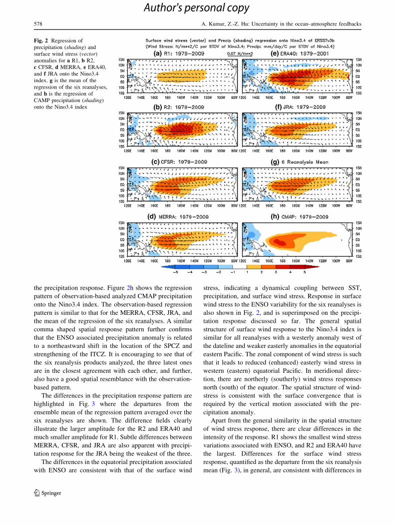
the precipitation response. Figure 2h shows the regression

pattern of observation-based analyzed CMAP precipitation

onto the Nino3.4 index. The observation-based regression

pattern is similar to that for the MERRA, CFSR, JRA, and

the mean of the regression of the six reanalyses. A similar

comma shaped spatial response pattern further confirms

that the ENSO associated precipitation anomaly is related

to a northeastward shift in the location of the SPCZ and

strengthening of the ITCZ. It is encouraging to see that of

the six reanalysis products analyzed, the three latest ones

are in the closest agreement with each other, and further,

also have a good spatial resemblance with the observation-

based pattern.

The differences in the precipitation response pattern are

highlighted in Fig. 3 where the departures from the

ensemble mean of the regression pattern averaged over the

six reanalyses are shown. The difference fields clearly

illustrate the larger amplitude for the R2 and ERA40 and

much smaller amplitude for R1. Subtle differences between

MERRA, CFSR, and JRA are also apparent with precipi-

tation response for the JRA being the weakest of the three.

The differences in the equatorial precipitation associated

with ENSO are consistent with that of the surface wind

stress, indicating a dynamical coupling between SST,

precipitation, and surface wind stress. Response in surface

wind stress to the ENSO variability for the six reanalyses is

also shown in Fig. 2, and is superimposed on the precipi-

tation response discussed so far. The general spatial

structure of surface wind response to the Nino3.4 index is

similar for all reanalyses with a westerly anomaly west of

the dateline and weaker easterly anomalies in the equatorial

eastern Pacific. The zonal component of wind stress is such

that it leads to reduced (enhanced) easterly wind stress in

western (eastern) equatorial Pacific. In meridional direc-

tion, there are northerly (southerly) wind stress responses

north (south) of the equator. The spatial structure of wind-

stress is consistent with the surface convergence that is

required by the vertical motion associated with the pre-

cipitation anomaly.

Apart from the general similarity in the spatial structure

of wind stress response, there are clear differences in the

intensity of the response. R1 shows the smallest wind stress

variations associated with ENSO, and R2 and ERA40 have

the largest. Differences for the surface wind stress

response, quantified as the departure from the six reanalysis

mean (Fig. 3), in general, are consistent with differences in

Fig. 2 Regression of

precipitation (shading) and

surface wind stress (vector)

anomalies for a R1, b R2,

c CFSR, d MERRA, e ERA40,

and f JRA onto the Nino3.4

index. g is the mean of the

regression of the six reanalyses,

and h is the regression of

CAMP precipitation (shading)

onto the Nino3.4 index

578 A. Kumar, Z.-Z. Hu: Uncertainty in the ocean–atmosphere feedbacks

123

Author's personal copy

precipitation response. Larger precipitation response in R2

and ERA40 is associated with a larger wind stress

response, while smaller precipitation response in R1 leads

to a smaller wind stress response. This implies a good

internal consistency between precipitation and wind stress

response for each reanalysis system in that larger negative

(positive) precipitation departures associated with larger

surface divergence (convergence) (not shown) lead to lar-

ger surface wind stress. We should point out that differ-

ences in wind stress, in addition, could also be associated

with differences in the parameterization of boundary layer

processes in the assimilation models. We also note that, as

for the precipitation, difference in wind stress response is

the smallest among the MERRA, CFS, and JRA.

3.2 Thermodynamical feedback

The surface heat fluxes over the ocean are the fields with less

direct measurements. Their variability is only indirectly

constrained by the meteorological observations in data

assimilation systems. As a result, in the reanalysis products

these quantities are likely more ‘‘model-dependent’’ than

other variables, such as the wind and temperature etc. Given

the central role played by surface fluxes in the ocean–

atmosphere feedbacks and ENSO evolution (e.g. Barnett

et al. 1991), as well as the fact that more and more studies are

using the surface fields from various analyses to examine the

mechanisms of ocean–atmosphere interactions and validate

model simulation, it is important to quantify uncertainties

inherent in reanalysis products. The connection of interan-

nual variability in the Nino3.4 index with different compo-

nents of the surface heat flux component is discussed next.

For all reanalyses the response in sensible and long-wave

heat flux is quite small and is not discussed here.

The response for the latent heat flux shown in Fig. 4 and

the sign convention is such that negative values represent

increased evaporation and cooling of the ocean. Increased

latent heat flux in response to warm SST (Fig. 1) implies a

negative feedback and has been noted in earlier studies

(e.g. Barnett et al. 1991). The latent heat flux response is

largest in the eastern equatorial Pacific between 100� and

140�W and slightly south of the equator for all reanalyses.

There is also a secondary maximum north of the equator

along 10�N shifted westward of its southern counterpart.

Much weaker latent heat flux response with a large spread

for different reanalysis products occurs in the western

Pacific: some products have positive anomalies (CFSR,

JRA), some have negative anomalies (R1, R2), while

Fig. 3 Regression of

precipitation (shading) and

surface wind stress (vector)

anomalies for a R1, b R2,

c CFSR, d MERRA, e ERA40,

and f JRA onto the Nino3.4

index. All the results are the

departure from the mean of the

regression of the six reanalyses

A. Kumar, Z.-Z. Hu: Uncertainty in the ocean–atmosphere feedbacks 579

123

Author's personal copy

others have almost no response (MERRA, ERA40). Such

differences either reflect a weak ENSO related signal or

may be due to the complexity of the thermodynamical

processes in the tropical western Pacific associated with

ENSO that are not well captured by the assimilation

models.

Compared with the regressions of the individual rea-

nalyses (Fig. 4a–f), the mean regression of the six reanal-

yses has a remarkable similarity to the regression with the

OAFlux both in the spatial pattern and the amplitude,

particularly in the central and eastern Pacific Ocean

(Fig. 4g, h), suggesting the potential advantage of using the

ensemble mean of the reanalyses in representing the latent

heat flux process associated with ENSO. The strength of

the negative feedback varies across different reanalyses and

the maximum south of the equator is *15–25 W/m2/�C per

unit standard deviation (STDV) of the NINO3.4

index, while the maximum north of the equator is

*5–15 W/m2/�C per unit STDV of the NINO3.4 index.

The percentages of the total variances of the latent heat flux

explained by the part related to Nino3.4 are very close in

different reanalyses and vary from 5.9% (R1) to 7.4%

(CFSR) for the average in the whole domain. However, all

these percentages are slightly lower than that of OAFlux

(7.9%).

The spatial structure of the latent heat flux response may

be explained with the help of the climatological wind stress

(Fig. 5). In the Southern Hemisphere, climatological mean

southeasterly trades are strongest in the eastern Pacific

(Fig. 5) and the direction of ENSO related surface wind

(as implied by the surface wind stress response, Fig. 2)

enhances the trades. Larger surface wind leads to increased

surface evaporation, cooling the ocean, damping the posi-

tive SSTA in the eastern tropical Pacific Ocean. A similar

argument holds for the secondary maximum north of the

equator along 10�N and its westward shift as the trades are

also shifted westward compared to their location for the

maximum in the Southern Hemisphere. In the western

Pacific, the wind response is opposite to the mean surface

wind climatology, leading to either a reduction in surface

wind speed, or resulting in a total reversal of surface wind

direction altogether. The uncertainty of the wind speed

changes in the reanalysis products may also explain the

divergence of the results of the latent heat flux associated

with ENSO in the western Pacific Ocean (Fig. 4). How-

ever, Fu et al. (1992) and Lloyd et al. (2011) argued that

Fig. 4 Regression of net latent

heat flux anomalies (contour)

for a R1, b R2, c CFSR,

d MERRA, e ERA40, f JRA,

and h OAFlux onto the Nino3.4

index, and g mean of regression

of the six reanalyses. The

shading represents the

corresponding departure from

the mean of the regression of the

six reanalyses in (a–f) and the

departure of the mean of

regression of the six reanalyses

from that of OAFlux in (g).

Downward (upward) is positive

(negative). Contour interval is

5 W/m2/�C per unit STDV of

the Nino3.4 index. The

percentages of the total net

latent heat flux variance

explained by the regression

averaged in the whole domain

are shown in each panel

580 A. Kumar, Z.-Z. Hu: Uncertainty in the ocean–atmosphere feedbacks

123

Author's personal copy

this latent heat flux feedback is actually driven by changes

in the near-surface specific humidity difference and the

winds play a secondary role

The response in the net downward shortwave (SW) flux

is shown in Fig. 6. The spatial structure of the SW response

is similar to that for the precipitation (Fig. 2) indicating

that the changes in cloudiness associated with precipitation

are responsible. In comparison with the latent heat

response, the SW response has a wider spatial extent, and

the largest anomalies are located westward. Negative val-

ues, implying reduced SW flux into the ocean, also repre-

sent a negative feedback for positive SSTAs associated

with ENSO (Fig. 1). The amplitude of the SW response

between reanalyses varies from -10 to -30 W/m2/�C per

unit STDV of the NINO3.4 index (Fig. 6). ERA40 has the

strongest overall damping, and CFSR the weakest. This is

consistent with Cronin et al. (2006) in that the cloud

forcing in ERA40 is too large in the ITCZ and equatorial

regions compared with buoy observations. The percentages

of the total variances of SW explained by the part linked

with the Nino3.4 are different between the analyses and

vary from 4.2% (R2) to13.6% (ERA40) for the average in

the whole domain. The mean of the percentage of the six

reanalyses is 8.2%, which is comparable with that for the

ISCCP (8.5%). Furthermore, the spatial pattern of the mean

of regression of the six reanalyses (Fig. 6g), as well as JRA

and ERA40 (Fig. 6e, f), are closer to the ISCCP (Fig. 6h)

than compared to the other four individual reanalyses

(Fig. 6a–d), particularly in the central Pacific Ocean,

although some differences in the amplitude are noted.

Although the precipitation response for MERRA, CFSR,

and JRA have a similar spatial structure and amplitude, the

corresponding SW response displays many differences in

the spatial distribution (Fig. 6). For example, MERRA and

JRA have a maximum damping west of the dateline, for the

CFSR SW anomaly has a more elongated structure. CFSR

also has a well defined band of positive SW response

extending from the west coast of South America to the

dateline along 5�N. Consistent with the largest precipita-

tion response in ERA40, the SW response is also the

largest, while the latent heat flux response was on the

weaker side (Fig. 4).

For different reanalyses and for observations the rela-

tionship between the variability in precipitation and SW is

confirmed by the scatter plots between the regressions of

the precipitation and surface SW anomalies on the Nino3.4

Fig. 5 Climatological mean of

surface wind stress (vector) and

precipitation (shading) for a R1,

b R2, c CFSR, d MERRA,

e ERA40, and f JRA. g is the

mean of the six reanalyses, and

h is the mean of CAMP

precipitation

A. Kumar, Z.-Z. Hu: Uncertainty in the ocean–atmosphere feedbacks 581

123

Author's personal copy

index (Fig. 7). The scatter plots are for all the points

located in 15�S–15�N, 120�E–75�W. Consistent with spa-

tial distribution patterns of the precipitation and SW radi-

ation regressions (Figs. 2, 3, 6), R1 has the smallest range

for SW radiation and precipitation anomalies, and ERA40

the largest, suggesting the weakest (strongest) radiation

damping of SSTA in R1 (ERA40). It is also noted that R1,

ERA40, and JRA (Fig. 7a, e, f) have a stronger linear

relation between SW radiation and precipitation anomalies,

which is similar to that between the ISCCP SW radiation

and CMAP precipitation (Fig. 7g), and R2 and CFSR have

the weakest ones. The differences among various reanal-

yses may be due to differences in parameterization

schemes among different atmospheric models that are part

of the reanalysis systems and dependence of cloudiness

amount on changes in precipitation.

Figure 8 shows the response to ENSO SST for the total

heat flux which is the sum of latent, sensible, SW, and

long-wave heat flux (with latent and SW having the largest

contribution). In general, the negative heat flux response

stretches along the equator from 160oE to the west coast

of South America. This is a consequence of the

complementary nature of the spatial pattern for the SW and

latent heat flux, while the former has maximum anomaly

near the dateline, and the latter is largest in the eastern

Pacific. The negative heat flux anomalies stretch along the

entire extent of the ENSO SST anomalies (Fig. 1), and act

as a damping term throughout the Pacific basin. Of all the

reanalyses the weakest heat flux damping is for the

MERRA and is split into two centers—one in the west

associated with the SW flux and one in the eastern Pacific

associated with the latent heat flux with a minimum in

between.

For all the reanalyses, the maximum damping due to the

net heat flux is around 25 W/m2/�C per unit STDV of the

NINO3.4 index. On the other hand, the spatial structure has

large differences. For some, the maximum is located in the

eastern Pacific (e.g. R1, CFSR and JRA), for ERA40 it has

an elongated structure, for R1 and R2 the maximum is

located more westward, while for MERRA there are two

distinct centers. Overall, the distribution pattern and

amplitude of R1, CFSR, and JRA are more similar to the

ensemble mean of the six reanalyses, compared with other

three reanalyses (R2, MERRA, and ERA40). Differences

Fig. 6 Regression of net short-

wave radiation anomalies at

surface (contour) for a R1,

b R2, c CFSR, d MERRA,

e ERA40, f JRA, and g ISCCP

onto the Nino3.4 index, and

g mean of regression of the six

reanalyses. The shading

represents the corresponding

departure from the mean of the

regression of the six reanalyses

in (a–f) and the departure of the

mean of regression of the six

reanalyses from that of ISCCP

in (g). Downward (upward) is

positive (negative). Contour

interval is 5 W/m2/�C per unit

STDV of the Nino3.4 index.

The percentages of the total

short-wave radiation variances

explained by the regression

averaged in the whole domain

are shown in each panel

582 A. Kumar, Z.-Z. Hu: Uncertainty in the ocean–atmosphere feedbacks

123

Author's personal copy

in spatial structure point to the level of uncertainty in the

reanalysis based estimates of the air–sea thermodynamical

feedback terms related to ENSO.

Figure 8g shows the ensemble mean of the regressions

of the six reanalyses of the total heat flux onto the Nino3.4

index (contours) and uncertainty (STDV of the departure

from the ensemble mean) (shading). The ensemble mean in

the eastern Pacific is approximately 25 W/m2/�C per unit

STDV of the NINO3.4 index with uncertainty of about

3 W/m2/oC per unit STDV of the NINO3.4 index. The

largest uncertainty is about 6–8 W/m2/�C per unit STDV of

the NINO3.4 index between 160 and 140�W. Farther west

the uncertainty is about the same order as the ensemble

mean and similar is true in the far eastern Pacific where the

uncertainty is even larger than the ensemble mean. The

ratio of the ensemble mean to the uncertainty shown in

Fig. 8h provides an estimate of the robustness in the esti-

mate of the heat flux feedback across different reanalyses.

The maximum absolute values of the ratios are in the

eastern Pacific between 90 and 130�W with absolute values

larger than 6, indicating more confidence in the value of the

thermodynamical damping in the eastern than in the wes-

tern Pacific. Nevertheless, in the western Pacific, the

uncertainties of the latent heat flux, net SW radiation, as

well as the total heat flux associated with ENSO in the

different reanalysis products (Figs. 4, 6, 8) are so large, the

robust conclusions about the feedback between ocean–

atmosphere cannot be made.

3.3 A synthesis of dynamical and thermodynamical

feedbacks

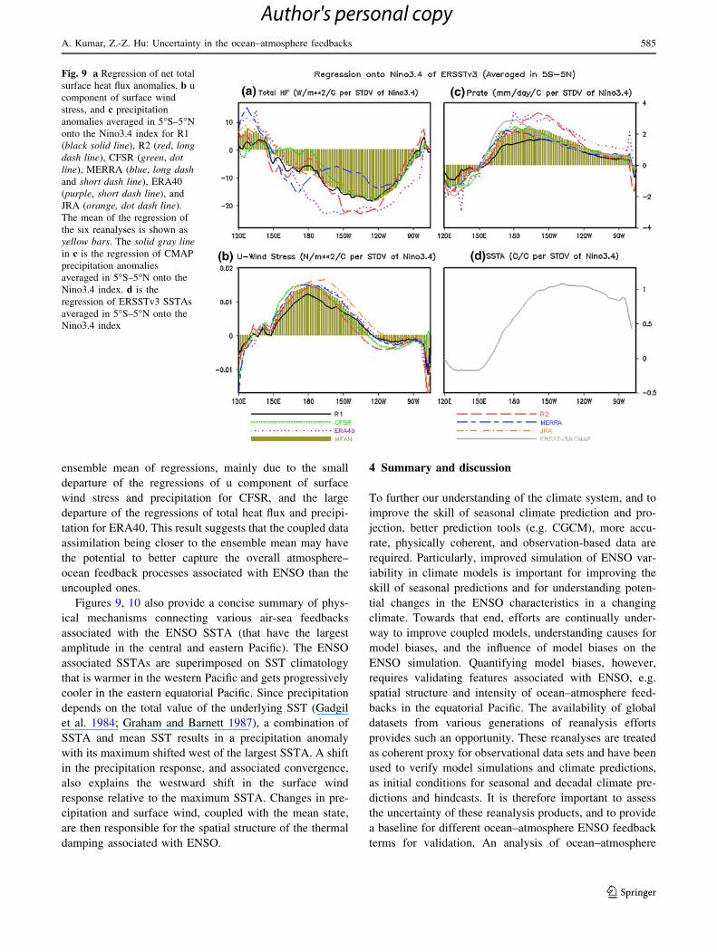
Figure 9 summarizes the longitudinal variation of the

regressions of the total heat flux (Fig. 9a), u component of

surface wind stress (Fig. 9b), precipitation (Fig. 9c), and

ERSSTv3 SST anomalies (Fig. 9d) averaged between 5�S

and 5�N on the Nino3.4 index. The corresponding regres-

sions of CMAP precipitation (gray line in Fig. 9c), as well

as the ensemble mean of the regression of the six reanalysis

products (bar graphs) are also included in the corresponding

panels (Fig. 9a–c). To further quantify comparison across

the six reanalyses, Fig. 10a–c show the mean of regressions

of the total heat flux anomalies averaged in (5�S–5�N,

150�E–90�W), u component of surface wind stress anom-

alies averaged in (5�S–5�N, 150�E–135�W), and precipi-

tation anomalies averaged in (5�S–5�N, 150�E–90�W) on

the Nino3.4 index. The different regions for different vari-

ables are chosen in order to focus on regions of that have

Fig. 7 Scatter of the regressions of net short-wave radiation anom-

alies (shown in 6) and the regressions of precipitation anomalies

(shown in Fig. 2) for a R1 a, b R2, c CFSR, d MERRA, e ERA40,

f JRA, and g ISCCP/CMAP in the region (15�S–15�N, 120�E–75�W).

Downward (upward) is positive (negative) for the net short-wave

radiation

A. Kumar, Z.-Z. Hu: Uncertainty in the ocean–atmosphere feedbacks 583

123

Author's personal copy

strongest connection with ENSO. The values plotted are

relative to the ensemble mean of the regressions of the six

reanalyses, and values close to (far from) zero indicate

proximity (large departure) from the ensemble mean.

For the regression of the total heat flux (Fig. 9a), the

ensemble mean value is negative from 150�E to the

west coast of South America and has an amplitude of

*20 W/m2/�C per unit STDV of the NINO3.4 index

between 150 and 120�W. The opposite phase relationship

with the SSTA shows that the total heat flux (Fig. 9a) is

clearly a damping for the SSTA (Fig. 9d). Overall, R1, R2,

and JRA are closer to the ensemble mean, and CFSR,

MERRA, and ERA40 have larger differences from the

ensemble mean (Fig. 10a). The estimates from CFSR and

MERRA have the least heat flux damping while ERA40

has the largest.

For the regression of precipitation (Figs. 9c, 10c),

CFSR, MERRA, and JRA are closer to the ensemble mean,

and ERA40 and R2 (R1) have larger positive (negative)

differences from the ensemble mean. In further comparison

with CMAP and the ensemble mean, CFSR is the closest

one, and ERA40, R2, and R1 have the largest difference.

Overestimated precipitation in ERA40 and R2 are consis-

tent with the excessive damping of the total heat flux

(Fig. 10a, c). The underestimated precipitation in R1 is

consistent with weak zonal wind stress (Figs. 9b, 10b). For

the regressions of u component of surface wind stress

(Fig. 9b) on the Nino3.4 index, CFSR, MERRA, and

ERA40 are the closest to the ensemble mean, and R1 (JRA)

has the largest negative (positive) differences from the

ensemble mean (Figs. 9c, 10c). We also note that near the

west coast of South America all reanalyses except for

CFSR have strong easterlies.

To quantify the degree of overall closeness of the

individual reanalyses to the ensemble mean of the six

reanalyses in capturing the feedback processes associated

with ENSO, we first compute the absolute values of the

regressions shown in Fig. 10a–c divided by the corre-

sponding spread between the six reanalyses. This is done

for the surface heat flux (Fig. 10a), zonal wind stress

(Fig. 10b), and precipitation (Fig. 10c) separately. For each

reanalysis we then sum the values for the three compo-

nents, and the result is shown in Fig. 10d. The smaller

(larger) number in Fig. 10d correspond to a smaller (larger)

departure from the overall mean of regressions of total heat

flux, u component of surface wind stress, and precipitation

anomalies from the ensemble mean. It is shown that CFSR

is the closest one and ERA40 is the farthest one to the

Fig. 8 Regression of net total

heat flux anomalies at surface

(contour) for a R1 a, b R2,

c CFSR, d MERRA, e ERA40,

and f JRA onto the Nino3.4

index. The shading in

(a–f) represents the

corresponding departure from

the mean of the regression of the

six reanalyses. g is the mean

(contour) and the spread

(shading) of the six reanalyses,

and h is the ratio of the mean to

the spread. Downward (upward)

is positive (negative). Contour

interval is 5 W/m2/�C per unit

STDV of the Nino3.4 index in

(a–g), and 2 in (h)

584 A. Kumar, Z.-Z. Hu: Uncertainty in the ocean–atmosphere feedbacks

123

Author's personal copy

ensemble mean of regressions, mainly due to the small

departure of the regressions of u component of surface

wind stress and precipitation for CFSR, and the large

departure of the regressions of total heat flux and precipi-

tation for ERA40. This result suggests that the coupled data

assimilation being closer to the ensemble mean may have

the potential to better capture the overall atmosphere–

ocean feedback processes associated with ENSO than the

uncoupled ones.

Figures 9, 10 also provide a concise summary of phys-

ical mechanisms connecting various air-sea feedbacks

associated with the ENSO SSTA (that have the largest

amplitude in the central and eastern Pacific). The ENSO

associated SSTAs are superimposed on SST climatology

that is warmer in the western Pacific and gets progressively

cooler in the eastern equatorial Pacific. Since precipitation

depends on the total value of the underlying SST (Gadgil

et al. 1984; Graham and Barnett 1987), a combination of

SSTA and mean SST results in a precipitation anomaly

with its maximum shifted west of the largest SSTA. A shift

in the precipitation response, and associated convergence,

also explains the westward shift in the surface wind

response relative to the maximum SSTA. Changes in pre-

cipitation and surface wind, coupled with the mean state,

are then responsible for the spatial structure of the thermal

damping associated with ENSO.

4 Summary and discussion

To further our understanding of the climate system, and to

improve the skill of seasonal climate prediction and pro-

jection, better prediction tools (e.g. CGCM), more accu-

rate, physically coherent, and observation-based data are

required. Particularly, improved simulation of ENSO var-

iability in climate models is important for improving the

skill of seasonal predictions and for understanding poten-

tial changes in the ENSO characteristics in a changing

climate. Towards that end, efforts are continually under-

way to improve coupled models, understanding causes for

model biases, and the influence of model biases on the

ENSO simulation. Quantifying model biases, however,

requires validating features associated with ENSO, e.g.

spatial structure and intensity of ocean–atmosphere feed-

backs in the equatorial Pacific. The availability of global

datasets from various generations of reanalysis efforts

provides such an opportunity. These reanalyses are treated

as coherent proxy for observational data sets and have been

used to verify model simulations and climate predictions,

as initial conditions for seasonal and decadal climate pre-

dictions and hindcasts. It is therefore important to assess

the uncertainty of these reanalysis products, and to provide

a baseline for different ocean–atmosphere ENSO feedback

terms for validation. An analysis of ocean–atmosphere

Fig. 9 a Regression of net total

surface heat flux anomalies, b u

component of surface wind

stress, and c precipitation

anomalies averaged in 5�S–5�N

onto the Nino3.4 index for R1

(black solid line), R2 (red, longdash line), CFSR (green, dotline), MERRA (blue, long dashand short dash line), ERA40

(purple, short dash line), and

JRA (orange, dot dash line).

The mean of the regression of

the six reanalyses is shown as

yellow bars. The solid gray linein c is the regression of CMAP

precipitation anomalies

averaged in 5�S–5�N onto the

Nino3.4 index. d is the

regression of ERSSTv3 SSTAs

averaged in 5�S–5�N onto the

Nino3.4 index

A. Kumar, Z.-Z. Hu: Uncertainty in the ocean–atmosphere feedbacks 585

123

Author's personal copy

feedback terms in the six reanalyses was presented in this

paper. The analysis provided the best estimate of feedback

terms as an average over all the products, and a discussion

of uncertainty in their estimates. Differences in ocean–

atmosphere feedback terms arise because of differences in

data assimilation systems, observational data, and param-

eterization schemes in the reanalysis models.

The overall structure and various ocean–atmosphere

dynamical and thermodynamical feedback terms agree well

in all the reanalyses and are likely due to the fact that all

the reanalyses agree on one basic premise: an increase in

precipitation in response to warm SST. Increased precipi-

tation, in turn, is associated with surface convergence and

an increase in cloudiness. Surface convergence then leads

to the basic structure of wind stress response, which, in

conjunction with its climatological mean, is responsible for

changes in the latent heat flux. Variability in cloudiness, in

turn, is responsible for changes in the shortwave radiation.

On the other hand, there are substantial differences in the

spatial structures of the ocean–atmosphere feedback terms

among reanalysis products, demonstrating the level of

uncertainty in current estimates arising from intrinsic dif-

ferences among reanalysis systems. For the regression of

the total heat flux, R1, CFSR, and JRA are closer to the

ensemble mean, and MERRA has the least heat flux

damping while ERA40 the largest.

The results also suggest that the coupled data assimila-

tion (CFSR) may have the potential to better capture the

overall atmosphere–ocean feedback processes associated

with ENSO than the uncoupled data assimilations. In the

‘‘coupled’’ assimilation system, where the first guess is

produced by a coupled GCM, seems to produce more

realistic response to SST anomalies. In particular, due to

the air–sea feedback and active SST adjustment, the net

surface heat flux represents less damping for ENSO. In

these uncoupled data assimilation systems, due to the fact

that atmospheric feedback on SST is prohibited, the

atmospheric state is the pure response to the SST with

Fig. 10 a Regression of net total surface heat flux anomalies

averaged in (5�S–5�N, 150�E–90�W), b u component of surface

wind stress anomalies averaged in (5�S–5�N, 150�E–135�W), and

c precipitation anomalies averaged in (5�S–5�N, 150�E–90�W) onto

the Nino3.4 index for the six reanalyses. The displayed regression is

the departure from the ensemble mean of the regressions of the six

reanalyses. d is the integrated absolute values of the regressions

shown in (a–c) divided by the corresponding spread of the regressions

of the six reanalyses. The units are W/m2/�C per unit STDV of the

Nino3.4 index in (a), N/m2/�C per unit STDV of the Nino3.4 index in

(b), mm/day/�C per unit STDV of the Nino3.4 index in (c)

586 A. Kumar, Z.-Z. Hu: Uncertainty in the ocean–atmosphere feedbacks

123

Author's personal copy

restriction of the assimilated observational data. As a

result, the dynamical and thermodynamical coupled pro-

cesses involved in ENSO cannot be fully described in

the uncoupled data assimilation systems, suggesting the

necessity of using a coupled assimilation system. If the

biases in the estimates from different reanalyses is con-

sidered random, and to the extent they average out, the

ensemble mean values for the wind stress and heat flux

response (e.g. Fig. 9) are our best estimate of the air–sea

feedback terms associated with the ENSO variability. Such

an estimate can be used to validate some features of ENSO

characteristics in model simulations, or validate other

reanalysis and observational products.

The regression patterns presented in this work are com-

puted over all seasons. However, considering the fact that

ENSO is an evolving, and a propagating phenomenon, with

a strong seasonal dependence, some of the features shown

in the regression patterns may have a strong seasonality. For

instance, on average, ITCZ anomaly associated with ENSO

displays a northwestward shift from boreal winter to sum-

mer (not shown). Nevertheless, this shift was not well

simulated in R1 and R2 (not shown). That may be a reason

of the lack of the comma-shaped rainfall structure in the all

season regression of R1 and R2 (Fig. 2). Moreover, the

larger uncertainty in the surface heat fluxes in the western

and central equatorial Pacific may be mainly associated

with the different characters of the eastward progression

during the ENSO developing phase in boreal summer in

various analyses. Overall, a seasonal dependence analysis

of the regression results may add additional information and

provide further validation for climate models.

Acknowledgments We appreciate the comments of Drs. Wanqiu

Wang, Yan Xue, D. G. DeWitt, and two reviewers. Thanks also go to

Dr. Li Zhang for managing the reanalysis data sets at CPC.

References

Barnett TP, Latif M, Kirk E, Roeckner E (1991) On ENSO physics.

J Clim 4(5):487–515

Barnston AG, Chelliah M, Goldenberg SB (1997) Documentation of a

highly ENSO-related SST region in the equatorial Pacific. Atmos

Ocean 35:367–383

Bjerknes J (1969) Atmospheric teleconnections from the equatorial

Pacific. Mon Weather Rev 97:163–172

Cronin MF, Bond NA, Fairall CW, Weller RA (2006) Surface cloud

forcing in the east Pacific stratus deck/cold tongue/ITCZ

complex. J Clim 19:392–409

Fu C, Fan H, Diaz H (1992) Variability in latent heat flux over the

tropical Pacific in association with recent two ENSO events. Adv

Atmos Sci 9:351–358

Gadgil S, Joseph PV, Joshi NV (1984) Ocean-atmosphere coupling

over monsoon regions. Nature 312:141–143

Graham NE, Barnett TP (1987) Sea surface temperature, surface wind

divergence, and convection over tropical oceans. Science

238:657–659

Guilyardi E et al (2004) Representing El Nino in coupled ocean–

atmosphere GCMs: the dominant role of the atmospheric

component. J Clim 17:4623–4629

Guilyardi E et al (2009a) Understanding El Nino in ocean–

atmosphere general circulation models: progress and challenges.

Bull Am Meterol Soc 90:325–340

Guilyardi E et al (2009b) Atmosphere feedbacks during ENSO in a

coupled GCM with a modified atmospheric convection scheme.

J Clim 22:5698–5718

IPCC (2007) Climate change 2007: the physical science basis. In:

Solomon S et al (eds) Contribution of working group I to the

fourth assessment report of the intergovernmental panel on

climate change. Cambridge University Press, Cambridge

Ji M, Kumar A, Leetmaa A (1994) A multiseason climate forecast

system at the National Meteorological Center. Bull Am Meterol

Soc 75:569–577

Kalnay E et al (1996) The NCEP/NCAR 40-year reanalysis project.

Bull Am Meterol Soc 77:437–471

Kanamitsu M et al (2002) NCEP-DOE AMIP-II reanalysis (R-2). Bull

Am Meterol Soc 83:1631–1643

Kim D, Kug J-S, Kang I-S, Jin F-F, Wittenberg AT (2008) Tropical

Pacific impacts of convective momentum transport in the SNU

coupled GCM. Clim Dyn 31:213–226

Kumar A, Zhang Q, Peng P, Jha B (2005) SST-forced atmospheric

variability in an atmospheric general circulation model. J Clim

18:3953–3967

Lloyd J, Guilyardi E, Weller H, Slingo J (2009) The role of

atmosphere feedbacks during ENSO in the CMIP3 models.

Atmos Sci Lett 10:170–176

Lloyd J, Guilyardi E, Weller H (2011) The role of atmosphere

feedbacks during ENSO in the CMIP3 models. Part II: using

AMIP runs to understand the heat flux feedback mechanisms.

Clim Dyn. doi:10.1007/s00382-010-0895-y (published on-line)

National Research Council (2010) Assessment of intraseasonal

to interannual climate prediction and predictability. The National

Academies Press, Washington, 192 pp, ISBN-10: 0-309-15183-X

Neelin JD et al (1998) ENSO theory. J Geophys Res 103:14261–

14290

Okumura YM, Deser C (2010) Asymmetry in the duration of El Nino

and La Nina. J Clim 23:5826–5843

Onogi K et al (2007) The JRA-25 reanalysis. J Meteorol Soc Jpn

85:369–432

Philander SGH (1990) El Nino, La Nina and the southern oscillation.

Academic Press, San Diego, 293 pp, ISBN 0125532350

Rasmusson EM, Carpenter TH (1982) Variation in tropical sea

surface temperature and surface wind fields associated with

Southern Oscillation/El Nino. Mon Weather Rev 110:354–384

Rienecker MM et al (2011) MERRA—NASA’s modern-era retro-

spective analysis for research and applications. J Clim

(submitted)

Saha S et al (2010) The NCEP climate forecast system reanalysis.

Bull Am Meterol Soc 91:1015–1057. doi:10.1175/2010BAM

S3001.1

Schneider EK (2002) Understanding differences between the equatorial

Pacific as simulated by two coupled GCMs. J Clim 15:449–469

Smith TM, Reynolds RW, Peterson TC, Lawrimore J (2008)

Improvements to NOAA’s historical merged land-ocean surface

temperature analysis (1880–2006). J Clim 21:2283–2296

Sun D et al (2006) Radiative and dynamical feedbacks over the

equatorial cold tongue: results from nine atmospheric GCMs.

J Clim 19:4059–4074

Sun D, Yu Y, Zhang T (2009) Tropical water vapor and cloud

feedbacks in climate models: a further assessment using coupled

simulations. J Clim 22:1287–1304

Uppala SM et al (2005) The ERA-40 re-analysis. Q J R Meterol Soc

131:2961–3012. doi:10.1256/qj.04.176

A. Kumar, Z.-Z. Hu: Uncertainty in the ocean–atmosphere feedbacks 587

123

Author's personal copy

Wang C, Picaut J (2004) Understanding ENSO physics—a review. In:

Wang C, Xie S-P, Carton JA (eds) Earth’s climate: the ocean–

atmosphere interaction. Geophysical Monograph Series, vol 147.

AGU, Washington, pp 21–48

Xie P, Arkin PA (1997) Global precipitation: a 17-year monthly

analysis based on gauge observations, satellite estimates, and

numerical model outputs. Bull Am Meterol Soc 78:2539–2558

Xue Y, Huang B, Hu Z-Z, Kumar A, Wen C, Behringer D, Nadiga S

(2011) An assessment of oceanic variability in the NCEP climate

forecast system reanalysis. Clim Dyn. doi:10.1007/s00382-

010-0954-4 (published online)

Yu L, Weller RA (2007) Objectively analyzed air–sea heat fluxes

(OAFlux) for the global ocean. Bull Am Met Soc 88:527–539

Zhang Y, Rossow W, Lacis A, Oinas V, Mishchenko M (2004)

Calculation of radiative flux profiles from the surface to top-of

atmosphere based on ISCCP and other global data sets:

refinements of the radiative transfer model and input data.

J Geophys Res 109:D19105. doi:10.1029/2003JD004457

588 A. Kumar, Z.-Z. Hu: Uncertainty in the ocean–atmosphere feedbacks

123

Author's personal copy