Verification of AROME-MetCoOp reanalysis for 2010

Application for the NBV project

Jakob Kristoffer Süld and Bruce Rolstad Denby

METreport

No. [x]/[xxxx] ISSN 2387-4201

Numerical weather prediction and air

pollution

Footer 2

METreport

Title Verification of AROME-MetCoOp reanalysis for 2010

Date 2015-04-26

Section Klimamodellering og luftforurensning (KL) and Numerisk værvarsling (NM)

Report no. No. [x]/[xxxx]

Author(s) Jakob Kristoffer Süld and Bruce Rolstad Denby

Classification ● Free ○ Restricted

Client(s) Miljødirektoratet

Client's reference

Abstract As part of the ‘Nasjonalt Beregningsvektøy for Lokal Luftkvalitet’ project (National modelling system for local air quality) the Norwegian Meteorological Institute (MET) has recalculated and archived meteorological model data for 2010 for all of Norway. The reanalysis was undertaken to provide the required 3D spatial meteorological fields needed for air quality model calculations to be carried out by the Norwegian institute for air research (NILU). The model used is the operative numerical weather prediction model AROME-MetCoOp, coupled to the surface model SURFEX. These models are part of the HARMONIE numerical weather predictions system. In this report verification of the 2.5 km resolution calculations for all of Norway for the entire year are presented along with a comparison with 1 km resolution calculations for Southern Norway for December 2010 only. The statistical analysis of the 2.5 km calculations shows that the model biases are generally very low for the meteorological parameters of 10 m wind, 2 m temperature and 12 hour accumulated precipitation. Hourly variability of the error is seasonally dependent, with the highest errors being found in the winter. The model reproduces very well the frequency distribution of these three meteorological parameters. Comparison of 2.5 and 1 km resolution calculations for Southern Norway show that in some instances the model provides improved wind results with the higher resolution calculations. These improvements are observed in complex terrain situations. Precipitation is not significantly affected by the enhanced resolution. The 1 km calculation led to an unexpected positive bias in temperature which may be the result of the surface model initialisation procedure.

Keywords AROME-MetCoOp, air quality, numerical weather prediction, verification

Disiplinary signature Responsible signature

Meteorologisk institutt Meteorological Institute Org.no 971274042 post@met.no

Oslo P.O. Box 43 Blindern 0313 Oslo, Norway T. +47 22 96 30 00

Bergen Allégaten 70 5007 Bergen, Norway T. +47 55 23 66 00

Tromsø P.O. Box 6314, Langnes 9293 Tromsø, Norway T. +47 77 62 13 00 www.met.no

Abstract

As part of the ‘Nasjonalt Beregningsvektøy for Lokal Luftkvalitet’ project (National modelling system for local air quality) the Norwegian Meteorological Institute (MET) has recalculated and archived meteorological model data for 2010 for all of Norway. The reanalysis was undertaken to provide the required 3D spatial meteorological fields needed for air quality model calculations to be carried out by the Norwegian institute for air research (NILU). The model used is the operative numerical weather prediction model AROME-MetCoOp, coupled to the surface model SURFEX. These models are part of the HARMONIE numerical weather predictions system. In this report verification of the 2.5 km resolution calculations for all of Norway for the entire year are presented along with a comparison with 1 km resolution calculations for Southern Norway for December 2010 only. The statistical analysis of the 2.5 km calculations shows that the model biases are generally very low for the meteorological parameters of 10 m wind, 2 m temperature and 12 hour accumulated precipitation. Hourly variability of the error is seasonally dependent, with the highest errors being found in the winter. The model reproduces very well the frequency distribution of these three meteorological parameters. Comparison of 2.5 and 1 km resolution calculations for Southern Norway show that in some instances the model provides improved wind results with the higher resolution calculations. These improvements are observed in complex terrain situations. Precipitation is not significantly affected by the enhanced resolution. The 1 km calculation led to an unexpected positive bias in temperature which may be the result of the surface model initialisation procedure.

Footer 4

Table of contents

1 Introduction 9

2 Climatological overview for 2010 10

3 Model description and setup 13 3.1 AROME physics 13 3.2 SURFEX as surface model 13 3.3 Model implementation and data assimilation 14 3.4 Boundaries and initialization of upper air fields 14 3.5 Model domains 15 3.6 Model run times and memory requirements 16 3.7 Special configuration for the 2010 reanalysis 16

4 Statistical analysis 17 4.1 Observations 17 4.2 Statistical error parameters 17

5 Verification results for all Norway 19 5.1 Monthly statistics for all of Norway 19 5.2 Frequency distribution and hit charts for all of Norway 22 5.3 Maps for all of Norway 25

6 Comparison of 2.5 and 1 km model calculations 29 6.1 Verification statistics for December in Southern Norway 29 6.2 Oslo time series for December 31 6.3 Bergen time series for December 33 6.4 Trondheim time series for December 34 6.5 Stavanger time series for December 35

7 Conclusions and recommendations 36 7.1 Conclusions concerning the model error verification results 36 7.2 Enhanced resolution 36 7.3 Verification methodology and parameters 37 7.4 Recommended model developments for further implementation 38

Acknowledgements 39

References 40

Appendix: List of archived model parameters 41

Footer 5

Footer 6

List of figures

Figure 1. Climatological overview of precipitation in Norway taken from Iden et al. (2010). 11

Figure 2. Climatological overview of 2 m temperature in Norway taken from Iden et al. (2010). 12

Figure 3. AROME-MetCoOp 2.5 km model domain and the reduced southern Norway 1 km domain used in the calculations. Shown is the topographic height. 15

Figure 5 Monthly mean error (top) and monthly standard deviation error (bottom) for hourly 10 m wind speed. Between 179-195 measurement sites are used in the analysis. 19

Figure 6 Monthly mean error (top) and monthly standard deviation error (bottom) for hourly 2 m temperature. Between 207-227 measurement sites are used in the analysis. 20

Figure 7 Monthly mean error (top) and monthly standard deviation error (bottom) for hourly 2 m temperature. Between 76-102 measurement sites are used in the analysis. 21

Figure 8. Summary plot of the data provided in Table 2. 22

Figure 9. Probability density functions for modelled and observed wind speed (top), temperature (middle) and precipitation (bottom). For wind speed the bin size is 0.5 m/s, for temperature 1 oC and for precipitation 0.1 mm.12hr. 23

Figure 10. Hit charts for wind speed (top) and precipitation (bottom). Colours indicate the positive hit diagonal (red) and the near positive hit (purple). Hits outside of these two regions (orange and green) should be as low as possible 24

Figure 11. Map of annual mean 10 m wind speed from AROME together with the Mean Error at measurement sites. Values are in m/s. 26

Figure 12. Map of annual mean 2 m temperature from AROME together with the Mean Error at measurement sites. Values are in oC. 27

Figure 13. Map of annual mean 12 hour accumulated precipitation from AROME together with the Mean Error at measurement sites. Values are given as mm/12hr. 28

Figure 14. Verification statistics for 10 m wind speed. Shown are the 2.5 km and 1 km AROME calculations for Southern Norway (119 sites) for December 2010. Also included for comparison is the 2.5 km AROME calculation for all of Norway (same results as presented in Figure 8). 30

Figure 15. Verification statistics for 2 m temperature. Shown are the 2.5 km and 1 km AROME calculations for Southern Norway (141 sites) for December 2010. Also included for comparison is the 2.5 km AROME calculation for all of Norway (same results as presented in Figure 8). 30

Figure 16. Verification statistics for 12 hour precipitation. Shown are the 2.5 km and 1 km AROME calculations for Southern Norway (77 sites) for December 2010. Also included for comparison is the 2.5 km AROME calculation for all of Norway (same results as presented in Figure 8). 31

Figure 17. Comparison of 2.5 (light blue) and 1 km (light green) AROME calculations for December 2010 at the synoptic measurement site Blindern. Data every 3 hours are shown for 10 m wind speed (top left), 10 m wind

Footer 7

direction (top right), 2 m temperature (bottom left)and 12 hour precipitation (bottom right).Precipitation is taken from the Tryvannshøgda site 32

Figure 18. Comparison of 2.5 (light blue) and 1 km (light green) AROME calculations for December 2010 at the synoptic measurement site Alna. Data every 3 hours are shown for 10 m wind speed (top left),10 m wind direction (top right),2 m temperature (bottom left). 32

Figure 19. Comparison of 2.5 (light blue) and 1 km (light green) AROME calculations for December 2010 at the synoptic measurement site Florida. Data every 3 hours are shown for 10 m wind speed (top left), 10 m wind direction (top right), 2 m temperature (bottom left)and 12 hour precipitation (bottom right). 33

Figure 20. Comparison of 2.5 (light blue) and 1 km (light green) AROME calculations for December 2010 at the synoptic measurement site Voll. Data every 3 hours are shown for 10 m wind speed (top left), 10 m wind direction (top right), 2 m temperature (bottom left)and 12 hour precipitation (bottom right). 34

Figure 21. Comparison of 2.5 (light blue) and 1 km (light green) AROME calculations for December 2010 at the synoptic measurement site Sola. Data every 3 hours are shown for 10 m wind speed (top left), 10 m wind direction (top right), 2 m temperature (bottom left)and 12 hour precipitation (bottom right). 35

Footer 8

List of tables

Table 1. Mathematical definitions of the statistical parameters used in the verification 18

Table 2. Total statistics for all sites and all hours 21

Footer 9

1 Introduction

As part of the ‘Nasjonalt Beregningsvektøy for Lokal Luftkvalitet’ project (National modelling system for local air quality) the Norwegian Meteorological Institute (MET) has recalculated and archived meteorological model data for 2010 for all of Norway. The reanalysis was undertaken to provide the required 3D spatial meteorological fields needed for air quality model calculations. The model used is the operative numerical weather prediction model AROME-MetCoOp, coupled to the surface model SURFEX. These models are part of the HARMONIE numerical weather forecasting system. In this report verification of the 2.5 km resolution calculations for all of Norway for the entire year is presented along with verification of the 1 km resolution calculations in Southern Norway for December only. Finally recommendations for further development and assessment are given.

Footer 10

2 Climatological overview for 2010

The year 2010 was characterised by lower temperatures and precipitation than normal, when compared to the reference period 1961-1990. An analysis of the climate for this year is provided in Iden et al. (2010). For 2010 the average temperature in Norway was 1 oC below normal. The average temperature was only above normal in parts of Finnmark and some coastal regions in Troms and Nordland and some arctic stations. Precipitation was on average 85% of normal. In some areas of Westland precipitation was 60-75% of normal and in in parts of Finnmark precipitation reached 125-150% of the norm. The general distribution of temperature and precipitation deviation from the norm for the entire year is shown in Figure 1 and Figure 2. In December, the period when both 1 km and 2.5 km calculations were made, the temperature was 4.7 oC below normal. The largest deviation occurred in elevated regions in southern Norway with temperatures of 10 oC below normal. The month December was also dry with only 55% of the normal precipitation for all of Norway. In Southern Norway this was as low as 10-20%. No climatological analysis of wind has been carried out for this year. In regard to air quality the year 2010 resulted in large exceedances of the air quality limit values in Stavanger, Bergen and Oslo. Particularly the hourly mean limit value for NO2 was exceeded due to episodes with low wind speeds, inversions and recirculation. These episodes have been assessed in more detail in Ødegård et al. (2011). 1 km calculations have been carried out for the December period in which a number of these exceedances occurred, and a comparison with observations, as well as with 2.5 km calculations, is presented in Section 6

Footer 11

Figure 1. Climatological overview of precipitation in Norway taken from Iden et al. (2010).

Footer 12

Figure 2. Climatological overview of 2 m temperature in Norway taken from Iden et al. (2010).

Footer 13

3 Model description and setup

A suite of experimental HARMONIE (Hirlam Aladin Research on Meso-scale Operational NWP in Euromed) models have been run at MET Norway since August 2008. This led to the implementation of AROME-Norway on yr.no on 1 October 2013. AROME-MetCoOp, which is run in cooperation between Swedish Meteorological and Hydrological Institute (SMHI) and MET Norway, replaced AROME-Norway on yr.no on 27 May 2014. The HARMONIE system includes several configuration options. The configuration used in this reanalysis is the AROME-MetCoOp (AM25) HARMONIE cycle 38h1.2 with AROME physics run on a 2.5 x 2.5 km2

grid. The same model configuration has been used for the 1 x 1 km2 domain. Both calculations use SURFEX as the surface interface model. The following subsections provide a brief description of this model configuration. More documentation is available concerning the modelling system on http://www.cnrm.meteo.fr/gmapdoc/ or through the HIRLAM homepage (HIRLAM, 2015).

3.1 AROME physics

AROME (Applications of Research to Operations at MEsoscale) is targeted for a horizontal resolution of 2.5 km or finer. It uses physical parameterizations based on the French academia model Meso-NH and the external surface model SURFEX. AROME has been operational at Météo-France since 18 December 2008, with a horizontal resolution of 2.5 km.

3.2 SURFEX as surface model

SURFEX (Surface externalisée) is developed at Météo-France and academia for offline experiments and introduced in NWP (Numerical Weather Prediction) models to ensure consistent treatment of processes related to the surface. SURFEX includes routines to simulate the exchange of energy and water between the atmosphere and 4 surface types (tiles); land, sea (ocean), lake (inland water) and town. The land or nature tile can be divided further into 12 vegetation types (patches). ISBA (Interaction between Soil Biosphere and Atmosphere) is used for modelling the land surface processes. Towns may be treated by a separate TEB (Town Energy Balance) module. Seas and lakes are also treated separately. The lake model, FLAKE (Freshwater LAKE), has recently been introduced in SURFEX. In the SURFEX configuration used in these calculations the four tiles are used but a single ‘average’ patch characteristic is used for each nature tile, rather than separation into individual patches for each tile. The global ECOCLIMAP-2 database which combines land cover maps and satellite information provides information about surface properties on 1 km resolution. The

Footer 14

orography is taken from gtopo30. “SURFEX Scientific Documentation” and “User’s Guide” are available on http://www.cnrm.meteo.fr/surfex/

3.3 Model implementation and data assimilation

The operational AROME-MetCoOp weather forecast model is updated each third hour; at 00, 03, 06, 09, 12, 15, 18 and 21 UTC using observations received in real-time from the global observing system. Forecasts are for 66 hours at every 6’th hour. For the reanalysis however, the model is updated every 6 hours; at 00, 06, 12 and 18 UTC. Model forecasts are made for 18 hours at 00 and 12 UTC.

3.3.1 Surface analysis

Surface analysis is performed by CANARI (Code d’Analyse Nécessaire à ARPEGE pour ses Rejets et son Initialisation). The analysis method is Optimal Interpolation and only conventional synoptic observations are used. 2 meter temperature and relative humidity observations are used to update the surface and soil temperature and moisture. The snow analysis is also performed with CANARI. Snow depth observations are used to update Snow Water Equivalent. The snow fields are analysed only at 06 UTC as there are very few snow depth observations at 00, 12 and 18. The Sea Surface Temperature is not analysed, but taken from the boundaries. ECMWF uses the OSTIA (Operational Sea Surface Temperature and Sea Ice Analysis) product, including SST from UK Met Office and SIC from MET. The surface temperature over sea ice is taken from the boundary model and remains unchanged through the forecast. The 1 km calculation uses blending and no surface assimilation. The initial surface fields of each forecast are read from the analysis of the 2.5 km model.

3.3.2 Upper air analysis

AROME-MetCoOp runs three dimensional variational (3DVAR) data assimilation using conventional observations from synop stations, ships, radiosondes and aircrafts. AMSU-A and AMSU-B/MHS data from the polar orbiting NOAA and METOP satellites are also used. For the reanalysis the 2.5km model uses blending instead of 3DVAR for the upper air assimilation.

3.4 Boundaries and initialization of upper air fields

AROME-MetCoOp 2.5 km receives its boundary values (1-hourly) from the ECMWF model at approximately 16 km horizontal resolution and 60 vertical levels. Model domains are initialised

Footer 15

with these fields. The 1 km calculation is nested into the 2.5 km runs and boundaries are updated every hour.

3.5 Model domains

Two model domains are applied. The first at 2.5 km resolution is the same as the operational AROME-MetCoOp model domain (738 x 947 grids) with 65 vertical levels. The second domain is the 1 km domain (438 x 708 grids) covering Southern Norway, also using 65 vertical levels. These domains are shown in Figure 3.

Figure 3. AROME-MetCoOp 2.5 km model domain and the reduced southern Norway 1 km domain used in the calculations. Shown is the topographic height.

Footer 16

3.6 Model run times and memory requirements

The reanalysis run was performed on the HPC (High Performance Computer) at ECMWF. With the setup used for the reanalysis at 2.5 km resolution the time needed for the calculations was roughly 1 week for every month of forecast. For the 1 km calculations roughly 10 days was required per month of calculation. One year of 2.5 km data requires 6.8TB of storage, or roughly 570 GB per month. One month for the 1 km model requires 310GB of storage.

3.7 Special configuration for the 2010 reanalysis

For the reanalysis, the model runs every 6 hours; at 00, 06, 12 and 18 UTC. Instead of the operational 66 hour forecasts 18 hour forecasts are made at 00 and 12, where the last 12 hours of each the forecasts are used as valid meteorological data. This configuration enables spin up times necessary for physical processes related to cloud formation and precipitation. Some schemes are different for the 1 km calculation compared to the 2.5 km calculations. For example the time stepping scheme used in the 1 km model is the predictor-corrector (PC) scheme. This scheme is somewhat less efficient than the SETTLS time stepping scheme, used in the 2.5 km runs, but has been implemented due to stability problems at 1 km. In addition to this, the major difference between the operational and reanalysis AROME-MetCoOp configurations is in the data assimilation methods, as previously indicated. The 2.5 km reanalysis uses blending instead of 3DVAR upper air assimilation and CANARI for surface assimilation (same as the operational AROME-MetCoOp). The 1km uses blending and no surface assimilation. The initial surface fields of each 1 km reanalysis forecast are read from the analysis of the 2.5 km model The meteorological parameters archived in the reanalysis differ from the operational AROME-MetCoOp calculations. A list of the archived parameters are provided in the Appendix. The major difference is that 3D spatial fields for the most important prognostic variables are archived.

Footer 17

4 Statistical analysis

All model forecasts in this report are verified against observations by interpolating (bilinear) the grid based forecasts to the observational sites. Verification is carried out for wind speed, temperature and precipitation based on statistical parameters that are regularly applied in other MET verification reports, see Bremnes and Homleid (2011) for a verification report of the year 2010 using the operational models then in place. For the application here the short forecast period (18 hours) does not require an assessment of the errors as a function of forecast time, as the statistical parameters vary little over this short period. Statistics are thus not shown as a function of the forecast hour but are aggregated into monthly statistics. Thus the last 12 hours for each of the 18 hour forecast are used to generate these statistics. The following assessments are shown

1. Monthly error statistics for 10 m wind speed, 2 m temperature and 12 hour accumulated precipitation.

2. Frequency distribution plots and hit charts for 10 m wind speed, 2 m temperature (no hit chart) and 12 hour accumulated precipitation.

3. Maps showing modelled mean 10 m wind speed, 2 m temperature and 12 hour accumulated precipitation together with mean errors at station sites

4. Statistical analysis and a selection of time series plots from the Southern Norway December period where both the 2.5 and 1 km models were run

4.1 Observations

All observations for the verification come from Klimadatavarehuset at MET and only synop stations are used. The number of available stations for comparison lies between 70 – 230 stations, dependent on the meteorological parameter. Not all stations have valid data through the entire year so the number of stations used for each hour also varies slightly.

4.2 Statistical error parameters

The verification statistics applied to continuous variables are standard in MET verification reports and defined in Table 1. For this report we present monthly values for the Mean Error (ME), which indicates the bias of the model, and the Standard Deviation of the Error (SDE), which indicates the distribution of the error around this mean (hourly uncertainty). The other statistical parameters of RMSE and MAE are only presented in the summary tables for the entire year.

Footer 18

Table 1. Mathematical definitions of the statistical parameters used in the verification

Footer 19

5 Verification results for all Norway

5.1 Monthly statistics for all of Norway

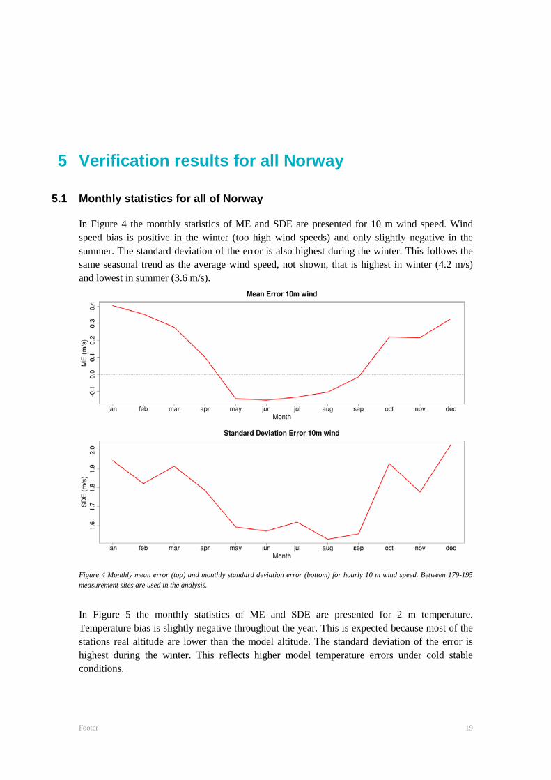
In Figure 4 the monthly statistics of ME and SDE are presented for 10 m wind speed. Wind speed bias is positive in the winter (too high wind speeds) and only slightly negative in the summer. The standard deviation of the error is also highest during the winter. This follows the same seasonal trend as the average wind speed, not shown, that is highest in winter (4.2 m/s) and lowest in summer (3.6 m/s).

Figure 4 Monthly mean error (top) and monthly standard deviation error (bottom) for hourly 10 m wind speed. Between 179-195 measurement sites are used in the analysis.

In Figure 5 the monthly statistics of ME and SDE are presented for 2 m temperature. Temperature bias is slightly negative throughout the year. This is expected because most of the stations real altitude are lower than the model altitude. The standard deviation of the error is highest during the winter. This reflects higher model temperature errors under cold stable conditions.

Footer 20

Figure 5 Monthly mean error (top) and monthly standard deviation error (bottom) for hourly 2 m temperature. Between 207-227 measurement sites are used in the analysis.

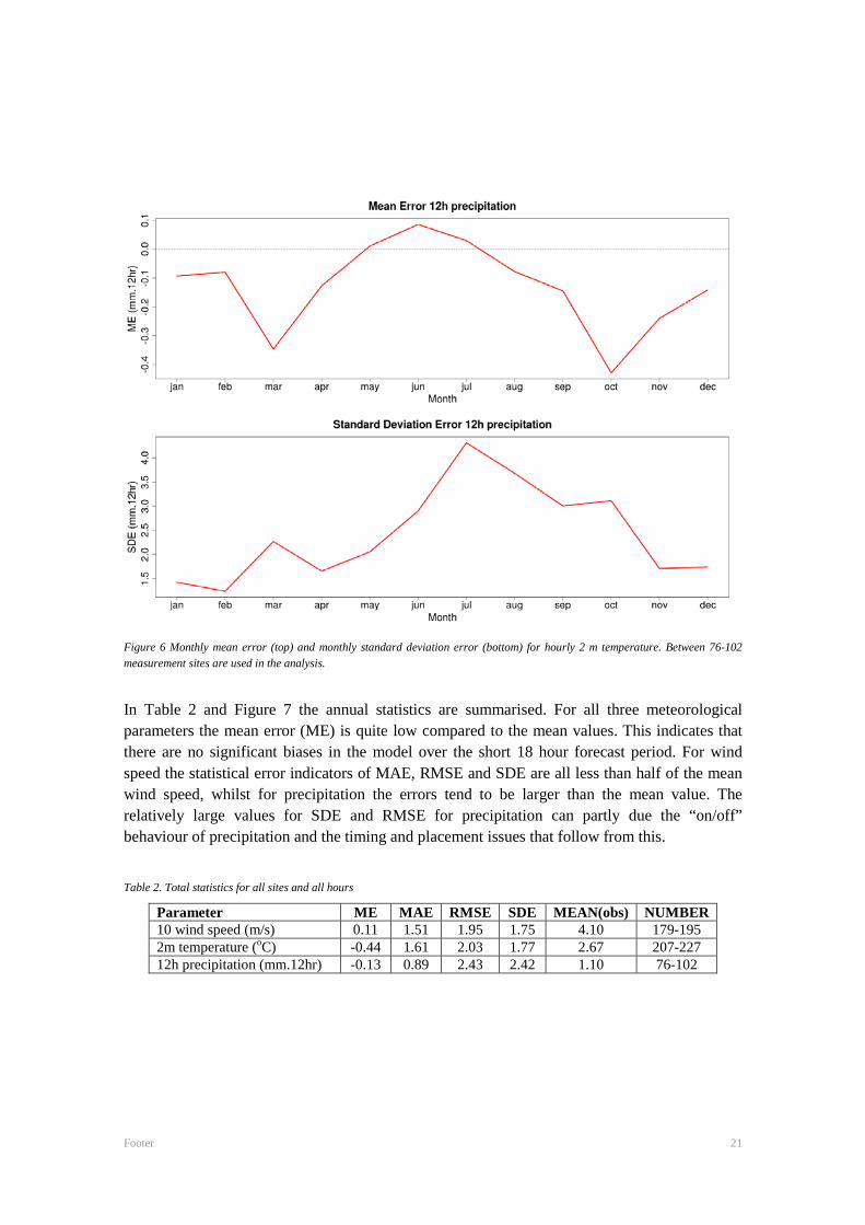
In Figure 6 the monthly statistics of ME and SDE are presented for 12 h precipitation. Precipitation bias is slightly negative during winter. The standard deviation of the error is highest during the summer-autumn period which also corresponds to the period with highest precipitation.

Footer 21

Figure 6 Monthly mean error (top) and monthly standard deviation error (bottom) for hourly 2 m temperature. Between 76-102 measurement sites are used in the analysis.

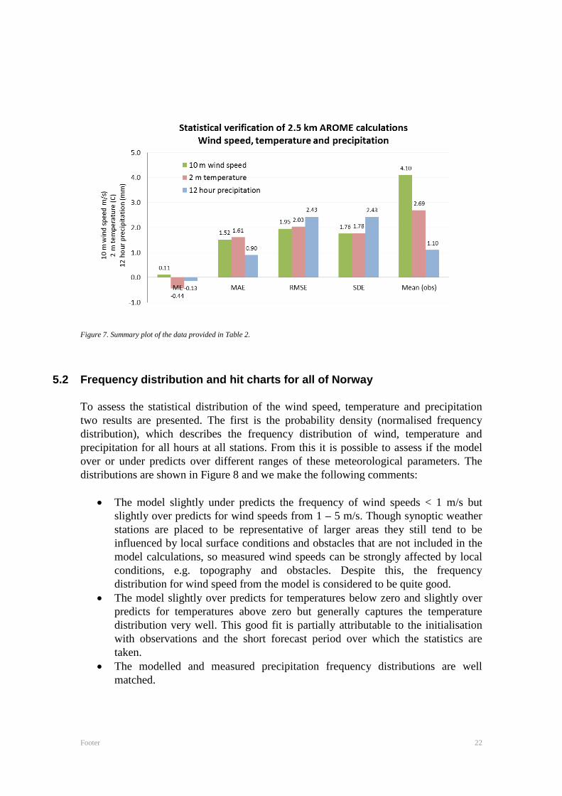
In Table 2 and Figure 7 the annual statistics are summarised. For all three meteorological parameters the mean error (ME) is quite low compared to the mean values. This indicates that there are no significant biases in the model over the short 18 hour forecast period. For wind speed the statistical error indicators of MAE, RMSE and SDE are all less than half of the mean wind speed, whilst for precipitation the errors tend to be larger than the mean value. The relatively large values for SDE and RMSE for precipitation can partly due the “on/off” behaviour of precipitation and the timing and placement issues that follow from this.

Table 2. Total statistics for all sites and all hours

Parameter ME MAE RMSE SDE MEAN(obs) NUMBER 10 wind speed (m/s) 0.11 1.51 1.95 1.75 4.10 179-195 2m temperature (oC) -0.44 1.61 2.03 1.77 2.67 207-227 12h precipitation (mm.12hr) -0.13 0.89 2.43 2.42 1.10 76-102

Footer 22

Figure 7. Summary plot of the data provided in Table 2.

5.2 Frequency distribution and hit charts for all of Norway

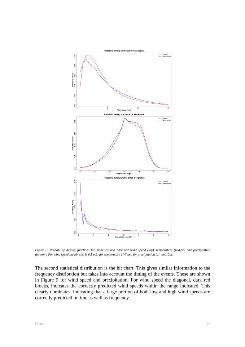
To assess the statistical distribution of the wind speed, temperature and precipitation two results are presented. The first is the probability density (normalised frequency distribution), which describes the frequency distribution of wind, temperature and precipitation for all hours at all stations. From this it is possible to assess if the model over or under predicts over different ranges of these meteorological parameters. The distributions are shown in Figure 8 and we make the following comments:

• The model slightly under predicts the frequency of wind speeds < 1 m/s but slightly over predicts for wind speeds from 1 – 5 m/s. Though synoptic weather stations are placed to be representative of larger areas they still tend to be influenced by local surface conditions and obstacles that are not included in the model calculations, so measured wind speeds can be strongly affected by local conditions, e.g. topography and obstacles. Despite this, the frequency distribution for wind speed from the model is considered to be quite good.

• The model slightly over predicts for temperatures below zero and slightly over predicts for temperatures above zero but generally captures the temperature distribution very well. This good fit is partially attributable to the initialisation with observations and the short forecast period over which the statistics are taken.

• The modelled and measured precipitation frequency distributions are well matched.

Footer 23

Figure 8. Probability density functions for modelled and observed wind speed (top), temperature (middle) and precipitation (bottom). For wind speed the bin size is 0.5 m/s, for temperature 1 oC and for precipitation 0.1 mm.12hr.

The second statistical distribution is the hit chart. This gives similar information to the frequency distribution but takes into account the timing of the events. These are shown in Figure 9 for wind speed and precipitation. For wind speed the diagonal, dark red blocks, indicates the correctly predicted wind speeds within the range indicated. This clearly dominates, indicating that a large portion of both low and high wind speeds are correctly predicted in time as well as frequency.

Footer 24

For precipitation the number of modelled and observed low level precipitation events dominates and are correctly predicted by the model. Note that non-precipitation is excluded from this analysis by setting the minimum value of the precipitation bin to 0.1 mm. Above levels of 2 mm the model performance is diminished. Predicting exact precipitation and its timing is demanding for any weather prediction model.

Figure 9. Hit charts for wind speed (top) and precipitation (bottom). Colours indicate the positive hit diagonal (red) and the near positive hit (purple). Hits outside of these two regions (orange and green) should be as low as possible

Footer 25

5.3 Maps for all of Norway

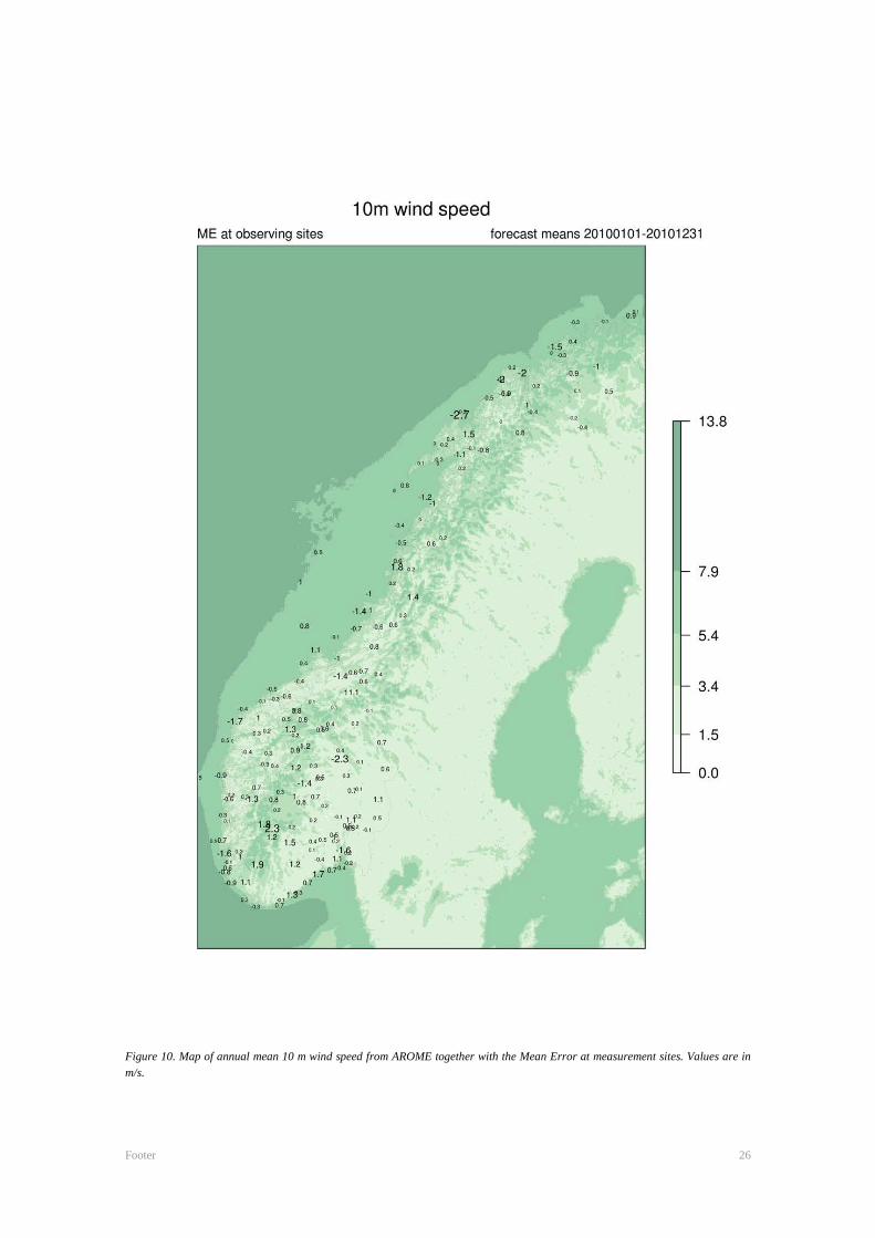
To indicate the geographical distribution of the errors, maps are made showing the mean model values as shaded pixels and the associated errors as values at measurement stations. These are shown for the mean model error (ME) for wind, temperature and precipitation. To aid visual interpretation the font size increases with increasing absolute error. The highest wind speeds (Figure 10) from the model are found at high elevation (intrusion into high elevation winds) and over water surfaces (low roughness lengths). There is no systematic geographical distribution of the error as this is most likely to be the result of local conditions affecting the measurement site. Temperature (Figure 11) is geographically related to height, latitude and proximity to the sea. Of these height plays a major role. The highest errors are found in mountainous regions where the elevation of the measurement site may not correspond to the model height at 2.5 km resolution. For production of temperature in public forecasts (yr.no) temperature is post processed to 500 m grids and this post processing technique takes into account height differences between model and observations. No post processing has been carried out on the model data here. Precipitation is geophysically related to orography and circulation patterns where the precipitation is highest on the west coast of Norway (Figure 12). The highest errors of around 2 mm/12hr are found on the west coast of Southern Norway. This error is equivalent to an annual precipitation error of approximately 700 mm. Total precipitation in this region is often more than 2000 mm.

Footer 26

Figure 10. Map of annual mean 10 m wind speed from AROME together with the Mean Error at measurement sites. Values are in m/s.

Footer 27

Figure 11. Map of annual mean 2 m temperature from AROME together with the Mean Error at measurement sites. Values are in oC.

Footer 28

Figure 12. Map of annual mean 12 hour accumulated precipitation from AROME together with the Mean Error at measurement sites. Values are given as mm/12hr.

Footer 29

6 Comparison of 2.5 and 1 km model calculations

In this section we present a comparison of the 2.5 and 1 km runs for the month of December. Two results are show, the overall statistics for all stations within the 1 km Southern Norway domain and a set of time series, every third hour is plotted, from a selection of stations within the cities of Oslo, Bergen, Stavanger and Trondheim. Wind speed, wind direction, temperature and precipitation are presented in these time series plots.

6.1 Verification statistics for December in Southern Norway

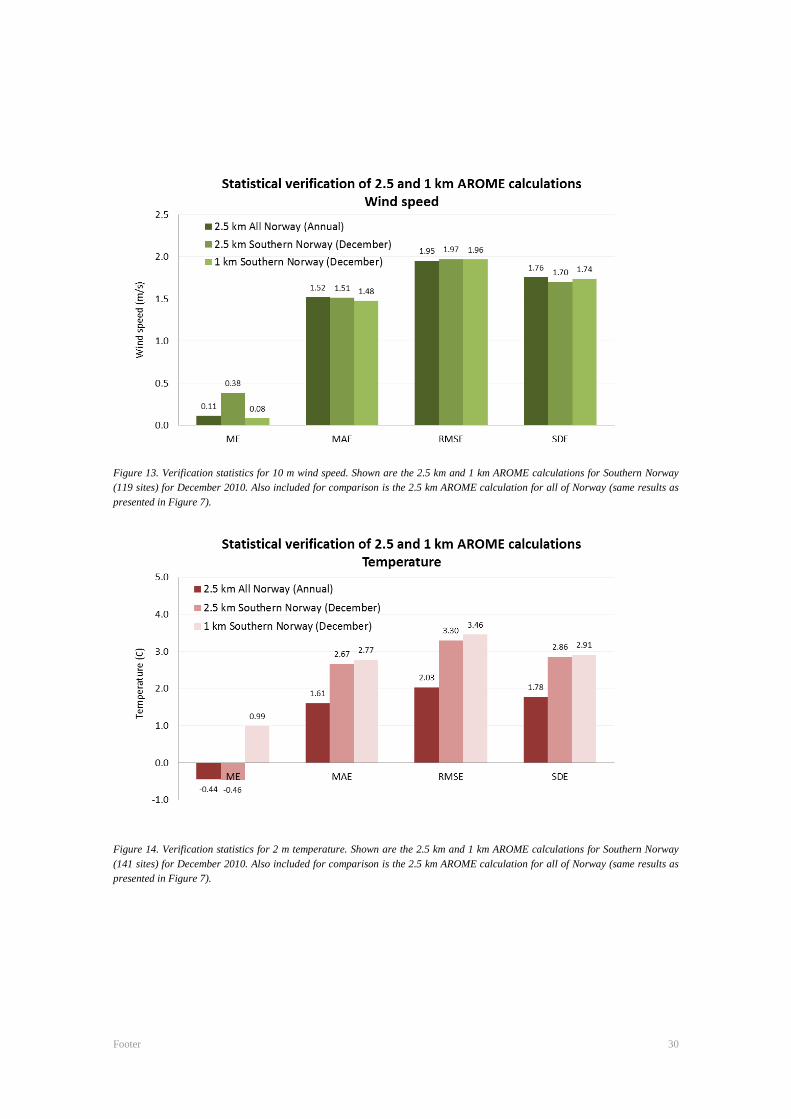
In Figure 13 - Figure 15 the same verification statistics that are presented in Figure 7 for all of Norway are also presented for the 2.5 and 1 km Southern Norway calculations for December, 2010. Included in these figures are the whole of Norway calculations for comparison. We make the following conclusions from this analysis

• The bias (ME) in wind speed is slightly reduced when increasing the model resolution from 2.5 to 1 km.

• There is no significant change in the other error statistics for wind speed when increasing the model resolution from 2.5 to 1 km.

• There is a significant positive bias (ME) for temperature when increasing the model resolution from 2.5 to 1 km.

• There is no significant change in the other error statistics for temperature when increasing the model resolution from 2.5 to 1 km.

• There is no significant difference in any of the precipitation error statistics when increasing the model resolution from 2.5 to 1 km.

The large change in model bias for temperature requires analysis. Though some of this change may be attributable to improved resolution of the topography it is also suspected that the surface assimilation method employed in the 1 km calculation is not optimal. For the Bedre Byluft forecasts (Denby et al., 2014; 2015), on which the 1 km calculation is based, surface observations are not directly assimilated into the system as they are done in the 2.5 km runs but instead the already assimilated 2.5 km surface variables are interpolated to the 1 km grid for initialisation. This may lead to a non-optimal initialisation of the 1 km calculation.

Footer 30

Figure 13. Verification statistics for 10 m wind speed. Shown are the 2.5 km and 1 km AROME calculations for Southern Norway (119 sites) for December 2010. Also included for comparison is the 2.5 km AROME calculation for all of Norway (same results as presented in Figure 7).

Figure 14. Verification statistics for 2 m temperature. Shown are the 2.5 km and 1 km AROME calculations for Southern Norway (141 sites) for December 2010. Also included for comparison is the 2.5 km AROME calculation for all of Norway (same results as presented in Figure 7).

Footer 31

Figure 15. Verification statistics for 12 hour precipitation. Shown are the 2.5 km and 1 km AROME calculations for Southern Norway (77 sites) for December 2010. Also included for comparison is the 2.5 km AROME calculation for all of Norway (same results as presented in Figure 7).

6.2 Oslo time series for December

Three stations (Blindern, Alna and Tryvannshøgda) are selected for Oslo. 3 hour time series data are presented in Figure 16 and Figure 17 for wind speed, wind direction and temperature for Blindern and Alna. Precipitation, not available at Blindern and Alna, is presented for Tryvannshøgda in Figure 16. Both the 2.5 and 1 km runs are shown. The following comments are made concerning these time series

• There is little difference between the 2.5 and 1 km calculations for wind speed and direction at the Blindern site.

• There is little difference between the 2.5 and 1 km calculations for wind speed at the Alna site.

• There is a difference between the 2.5 and 1 km calculations for wind direction at the Alna site. The 1 km run improves the wind direction for a significant amount of the December period. This is likely due to an improved representation of topography in this region allowing, for example, drainage flows and channelling to develop.

• The temperature is higher for the 1 km runs, compared to the 2.5 km calculation, for both Oslo sites. This reflects the positive temperature bias generally found in the 1 km runs.

• There is little difference between the 2.5 km and the 1 km precipitation. Events are well captured by both model resolutions though the intensities did not always match the available measurements. Precipitation events during this period were snow.

Footer 32

Figure 16. Comparison of 2.5 (light blue) and 1 km (light green) AROME calculations for December 2010 at the synoptic measurement site Blindern. Data every 3 hours are shown for 10 m wind speed (top left), 10 m wind direction (top right), 2 m temperature (bottom left)and 12 hour precipitation (bottom right).Precipitation is taken from the Tryvannshøgda site

Figure 17. Comparison of 2.5 (light blue) and 1 km (light green) AROME calculations for December 2010 at the synoptic measurement site Alna. Data every 3 hours are shown for 10 m wind speed (top left),10 m wind direction (top right),2 m temperature (bottom left).

Footer 33

6.3 Bergen time series for December

One station (Florida) is selected for Bergen. 3 hour time series are presented in Figure 18 for wind speed, wind direction, temperature and precipitation. Both the 2.5 and 1 km runs are shown. The following comments are made concerning these time series

• Wind speeds are lower and more realistic for the 1 km run during light wind periods. This site is centrally located in Bergen which is located in a valley approximately 2 km wide. Increased resolution appears to resolve some of the valley meteorological features.

• There are some differences between the 2.5 and 1 km calculations for wind direction at this site but these are not large.

• The temperature is slightly higher for the 1 km runs, compared to the 2.5 km calculation. This reflects the positive temperature bias generally found in the 1 km runs.

• Precipitation events and intensities are captured by both resolutions. These events were chiefly rain.

Figure 18. Comparison of 2.5 (light blue) and 1 km (light green) AROME calculations for December 2010 at the synoptic measurement site Florida. Data every 3 hours are shown for 10 m wind speed (top left), 10 m wind direction (top right), 2 m temperature (bottom left)and 12 hour precipitation (bottom right).

Footer 34

6.4 Trondheim time series for December

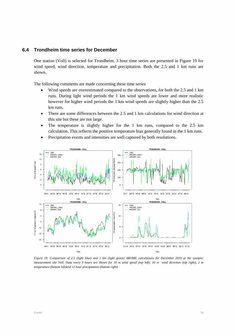
One station (Voll) is selected for Trondheim. 3 hour time series are presented in Figure 19 for wind speed, wind direction, temperature and precipitation. Both the 2.5 and 1 km runs are shown. The following comments are made concerning these time series

• Wind speeds are overestimated compared to the observations, for both the 2.5 and 1 km runs. During light wind periods the 1 km wind speeds are lower and more realistic however for higher wind periods the 1 km wind speeds are slightly higher than the 2.5 km runs.

• There are some differences between the 2.5 and 1 km calculations for wind direction at this site but these are not large.

• The temperature is slightly higher for the 1 km runs, compared to the 2.5 km calculation. This reflects the positive temperature bias generally found in the 1 km runs.

• Precipitation events and intensities are well captured by both resolutions.

Figure 19. Comparison of 2.5 (light blue) and 1 km (light green) AROME calculations for December 2010 at the synoptic measurement site Voll. Data every 3 hours are shown for 10 m wind speed (top left), 10 m wind direction (top right), 2 m temperature (bottom left)and 12 hour precipitation (bottom right).

Footer 35

6.5 Stavanger time series for December

One station (Sola) is selected for Stavanger. 3 hour time series are presented in Figure 20 for wind speed, wind direction, temperature and precipitation. Both the 2.5 and 1 km runs are shown. The following comments are made concerning these time series

• There is very little difference between the 2.5 and 1 km runs in terms of wind speed and wind direction. Sola is situated at Stavanger airport and is reasonably flat and exposed.

• There are some differences between the 2.5 and 1 km calculations for wind direction at this site but these are not large.

• The temperature is very similar for both the 1 km and 2.5 km runs. • Precipitation events and intensities are mostly captured by both resolutions, though

some precipitation is predicted that is not observed.

Figure 20. Comparison of 2.5 (light blue) and 1 km (light green) AROME calculations for December 2010 at the synoptic measurement site Sola. Data every 3 hours are shown for 10 m wind speed (top left), 10 m wind direction (top right), 2 m temperature (bottom left)and 12 hour precipitation (bottom right).

Footer 36

7 Conclusions and recommendations

7.1 Conclusions concerning the model error verification results

Verification of the standard synoptic meteorological parameters of 10 m wind, 2 m temperature and precipitation (12 hour accumulated) has been carried out. Between 100 and 200 synoptic stations have been used to determine a number of error statistics on a monthly basis. In particular the mean error (ME), that represents the bias in the model, and the standard deviation of the error (SDE), that represents model uncertainty on an hourly basis, has been assessed. Error statistics indicate satisfactorily low biases in all three meteorological parameters addressed but also show seasonal differences. Wind speeds are positively biased in winter and slightly negatively biased in summer, temperatures are slightly negatively biased throughout the year and precipitation has a slight negative bias in spring and autumn. Seasonally there is higher model uncertainty during the winter for wind speed and temperature but a higher uncertainty in precipitation during the summer/autumn. Higher uncertainty in wind and temperature during the colder winter months likely reflects the models decreased ability to reproduce the colder more stable conditions found then, though more attention to both the radiation and turbulence processes in the model are required to determine why this occurs. A comparison of modelled and observed frequency distributions for wind speed, temperature and precipitation show a very good statistical representation of these. The tendency of the model to slightly over predict the frequency of low wind speeds and low temperatures is reflected in the monthly error statistics, as these distributions are seasonally coupled.

7.2 Enhanced resolution

The comparison of 2.5 km and 1 km resolutions for the month of December 2010 indicates that wind speeds and directions at some sites can be improved with the use of higher resolution modelling. Improvements are found in areas with complex topography, though the comparison of two sites within the city of Oslo indicate that only one of these is improved using higher resolution. There is little to be gained by increasing the resolution where topography and land use characteristics vary little.

Footer 37

The final impact of enhanced resolution will need to be assessed by the air quality model itself. Air quality measurements provide information on the transport and dispersion of pollutants within the cities and correctly modelling these will provide verification of both the meteorological and air quality models.

7.3 Verification methodology and parameters

Verification has been carried out on standard synoptic station data of wind, temperature and precipitation. This report can then be compared to standard verification reports produced regularly at MET. However, for air quality applications there are other parameters and other methods for assessing model performance that may provide further insight into the quality of the model results. In particular it is the low wind speed conditions that are the most important for air quality. The ability of the model to reproduce low wind speeds has been addressed in the probability distributions and hit charts but the general error statistics will not reflect this, as they are strongly weighted by the errors associated with higher wind speeds. In addition the ability of the model to represent inversions is only partially addressed through temperature error statistics. A proper assessment of inversion strength would require comparisons with radiosonde data, boundary layer height measurements or with temperature measurements placed at different heights in the terrain. These data are scarce or non-existent in and around the cities addressed in this study. It is also worth noting that in the current air quality modelling system from NILU that upper air temperature inversions are not used. Stability and dispersion are determined solely by the surface flux conditions. Verification of local circulation patterns has also not been carried out, as there is no data available for this. This, together with inversions, are likely to be important for the air quality modelling. Indeed, taking the meteorological fields and applying them in an air quality model is another step in the verification process. Air quality measurements, that are strongly dependent on local dispersion conditions, contain relevant information for verification of the meteorological model as well as the air quality model. Other relevant model parameters for verification include humidity, radiation and turbulent fluxes. However, since these are non-standard parameters significant work is required to develop the routines for assessing these data. No attempt was made to use cross-validation techniques to verify the model. As such synoptic measurement data used to initialise the model are also used for the forecast validation. Even though the verification is made using the last 12 hours of the 18 hour forecast the influence of the initialisation will still be present in the forecast to some extent. Cross-validation using an assimilation and validation subset of synoptic stations may be implementable, but it may not provide more insight into the model performance and is not necessarily recommended.

Footer 38

7.4 Recommended model developments for further implementation

This verification study has indicated a number of areas of model development that need to be addressed. These include:

• Investigation and improvement of the land surface initialisation procedures for the 1 km nested model calculations.

• Testing and implementation of alternative time stepping and boundary condition schemes to improve stability and efficiency of the 1 km model.

• Assessment of the ECOCLIMAP database in cities to determine if the correct land use characteristics are provided for the selected cities.

• Assess the impact of resolution for the December 2010 period using air quality models for all relevant cities.

• Assess the feasibility of archiving operative weather forecasts for use in NBV instead of reanalysis. This will require updating model parameters and an automatic archiving system.

Footer 39

Acknowledgements

Thanks to Bjørg Jenny Kokkvoll Engdahl from MET for providing scripts and text from previous MET verification reports for adaption here.

Footer 40

References

Bremnes J.B. and M. Homleid (2011). Verification of Operational Numerical Weather Prediction Models December 2010 to February 2011. MET report 06/2011 http://met.no/Forskning/Publikasjoner/MET_report/2011/?module=Files;action=File.getFile;ID=4400 Denby B.R., Jacob Suld, Arne Kristensen, Ingrid Sundvor, Islen Vallejo Henao, Sam Erik Walker (2015). Bedre byluft: Endringer i 2014 og forskningsresultater av prognoser for meteorologi og luftkvalitet i norske byer vinteren 2013-2014. MET report 08/2015. http://met.no/Forskning/Publikasjoner/MET_report/?module=Files;action=File.getFile;ID=6391 Denby B.R., Anna Carlin Benedictow, Aslaug Skålevik Valved, Thomas Olsen, Arne Kristensen, Leiv Håvard Slørdal (2014). Bedre byluft - Prognoser for meteorologi og luftkvalitet i norske byer vinteren 2013 – 2014. Met report 17/2014 http://met.no/Forskning/Publikasjoner/MET_report/2014/?module=Files;action=File.getFile;ID=6321 HIRLAM 2015. Web site for HIRLAM, URLs: http://www.hirlam.org/index.php/hirlam-programme-53/general-model-description/mesoscale-harmonie http://www.hirlam.org/index.php/documentation/harmonie Iden K., Ketil Isaksen, Stein Kristiansen, Jostein Mamen, Hanna Szewczyk-Bartnicka (2011). Været i Norge Klimatologisk oversikt Året 2010. METinfo report Nr. 13/2010. http://www.met.no/Forskning/Publikasjoner/MET_info/2010/?module=Files;action=File.getFile;ID=6063

Ødegaard, V., Gjerstad, K.I., Abildsnes, H., Olsen, T. (2011). Bedre byluft: Prognoser for meteorologi og luftkvalitet i norske byer vinteren 2010-2011. Oslo, met.no (met.no report, 8/2011). http://met.no/Forskning/Publikasjoner/filestore/report8_2011.pdf

Footer 41

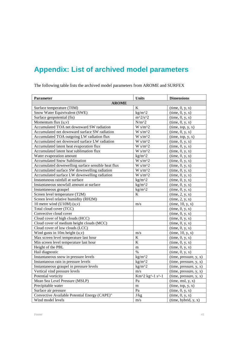
Appendix: List of archived model parameters

The following table lists the archived model parameters from AROME and SURFEX Parameter Units Dimensions

AROME Surface temperature (T0M) K (time, 0, y, x) Snow Water Equivivalent (SWE) kg/m^2 (time, 0, y, x) Surface geopotential (fis) m^2/s^2 (time, 0, y, x) Momentum flux (u,v) N/m^2 (time, 0, y, x) Accumulated TOA net downward SW radiation W s/m^2 (time, top, y, x) Accumulated net downward surface SW radiation W s/m^2 (time, 0, y, x) Accumulated TOA outgoing LW radiation flux W s/m^2 (time, top, y, x) Accumulated net downward surface LW radiation W s/m^2 (time, 0, y, x) Accumulated latent heat evaporation flux W s/m^2 (time, 0, y, x) Accumulated latent heat sublimation flux W s/m^2 (time, 0, y, x) Water evaporation amount kg/m^2 (time, 0, y, x) Accumulated Snow Sublimation W s/m^2 (time, 0, y, x) Accumulated downwelling surface sensible heat flux W s/m^2 (time, 0, y, x) Accumulated surface SW downwelling radiation W s/m^2 (time, 0, y, x) Accumulated surface LW downwelling radiation W s/m^2 (time, 0, y, x) Instantanous rainfall at surface kg/m^2 (time, 0, y, x) Instantaneous snowfall amount at surface kg/m^2 (time, 0, y, x) Instantaneous graupel kg/m^2 (time, 0, y, x) Screen level temperature (T2M) K (time, 2, y, x) Screen level relative humidity (RH2M) (time, 2, y, x) 10 metre wind (U10M) (u,v) m/s (time, 10, y, x) Total cloud cover (TCC) (time, 0, y, x) Convective cloud cover (time, 0, y, x) Cloud cover of high clouds (HCC) (time, 0, y, x) Cloud cover of medium height clouds (MCC) (time, 0, y, x) Cloud cover of low clouds (LCC) (time, 0, y, x) Wind gusts in 10m height (u,v) m/s (time, 10, y, x) Max screen level temperature last hour K (time, 0, y, x) Min screen level temperature last hour K (time, 0, y, x) Height of the PBL m (time, 0, y, x) Hail diagnostic % (time, 0, y, x) Instantaneous snow in pressure levels kg/m^2 (time, pressure, y, x) Instantanous rain in pressure levels kg/m^2 (time, pressure, y, x) Instantaneous graupel in pressure levels kg/m^2 (time, pressure, y, x) Vertical vind pressure levels m/s (time, pressure, y, x) Potential vorticity Km^2 kg^-1 s^-1 (time, pressure, y, x) Mean Sea Level Pressure (MSLP) Pa (time, msl, y, x) Precipitable water m (time, top, y, x) Surface air pressure Pa (time, 0, y, x) Convective Available Potential Energy (CAPE)" J/kg (time, 0, y, x) Wind model levels m/s (time, hybrid, y, x)

Footer 42

Air temperature model levels K (time, hybrid, y, x) Specific humidity model levels Kg/kg (time, hybrid, y, x) Atmospheric cloud condensed water content in model levels kg m-2 (time, hybrid, y, x) Cloud ice in model levels kg m-2 (time, hybrid, y, x) Cloud cover in model levels % (time, hybrid, y, x) Turbulent kinetic energy (TKE) m^2/s^2 (time, hybrid, y, x) Geopotential model levels m^2/s^2 (time, hybrid, y, x) Accumulated total precipitation kg/m^2 (time, 0, y, x) Total accumulated solid precipitation kg/m^2 (time, 0, y, x) Wind gust m/s (time, 10, y, x)

SURFEX Vegetation index (VEG) (time, 0, y, x) Sea surface temperature (SST) (time, 0, y, x) 2 m temperature (T2M) K (time, 2, y, x) 2 m specific humidity (Q2M) kg/kg (time, 2, y, x) 2 m relative humidity (HU2M) (time, 2, y, x) TG1 K (time, -, y, x) TG2 K (time, --, y, x) WG1 m^3/m^3 (time, -, y, x) WG2 m^3/m^3 (time, --, y, x) WGI1 m^3/m^3 (time, -, y, x) WGI2 m^3/m^3 (time, --, y, x) WSNOW_VEG1 kg/m^2 (time, 0, y, x) RSNOW_VEG1 kg/m^2 (time, 0, y, x) ASNOW_VEG (time, 0, y, x) LAI (time, 0, y, x) Roughness length momentum (Z0) m (time, 0, y, x) Roughness length temperature (Z0H) m (time, 0, y, x) RI (time, 0, y, x) CD W/s^2 (time, 0, y, x) CE W/s/K (time, 0, y, x) LE W/m^2 (time, 0, y, x) H W/m^2 (time, 0, y, x) Momentum flux (FM) (u,v) kg/ms^2 (time, 0, y, x) Net radiation (RN) W/m^2 (time, 0, y, x) Surface energy flux (GFLUX) W/m^2 (time, 0, y, x)