The Change in the ENSO Teleconnection under a Low Global Warming Scenario andthe Uncertainty due to Internal Variability

CLIO MICHEL AND CAMILLE LI

Geophysical Institute, University of Bergen and Bjerknes Centre for Climate Research, Bergen, Norway

ISLA R. SIMPSON

Climate and Global Dynamics Laboratory, National Center for Atmospheric Research, Boulder, Colorado

INGO BETHKE

Geophysical Institute, University of Bergen and Bjerknes Centre for Climate Research, Bergen, Norway

MARTIN P. KING AND STEFAN SOBOLOWSKI

NORCE Norwegian Research Centre AS and Bjerknes Centre for Climate Research, Bergen, Norway

(Manuscript received 27 September 2019, in final form 24 January 2020)

ABSTRACT

El Niño–SouthernOscillation (ENSO) is a main driver of climate variability worldwide, but the presence of

atmospheric internal variability makes accurate assessments of its atmospheric teleconnections a challenge.

Here, we use a multimodel large ensemble of simulations to investigate the ENSO teleconnection response

to a low global warming scenario that represents Paris Agreement targets. The ensemble comprises five

atmospheric general circulation models with two experiments (present-day and128C) in which the same set

of ENSO events is prescribed, which allows for quantification of the uncertainty in the ENSO response due to

internal variability. In winter, the teleconnection during the positive ENSO phase features a strong negative

anomaly in sea level pressure over the northeast Pacific (and vice versa for the negative phase); this anomaly

shifts northeastward and strengthens in the warming experiment ensemble. At least 50–75 ENSO events are

required to detect a significant shift or strengthening, emphasizing the need to adequately sample the internal

variability to isolate the forced response of the ENSO teleconnection under a low warming scenario. Even

more events may be needed if one includes other sources of uncertainty not considered in our experimental

setup, such as changes in ENSO itself. Over North America, precipitation changes are generally more

robust than temperature changes for the regions considered, despite large internal variability, and are shaped

primarily by changes in atmospheric circulation. These results suggest that the observational period is likely

too short for assessing changes in the ENSO teleconnection under Paris Agreement warming targets.

1. Introduction

El Niño–Southern Oscillation (ENSO) is a major

driver of climate variability on interannual time scales.

Anomalous sea surface temperatures (SSTs) in the

equatorial Pacific trigger an atmospheric teleconnec-

tion, usually described as a wave train from the tropics

to higher latitudes, related to the Pacific–NorthAmerican

teleconnection pattern (Wallace and Gutzler 1981), and

extending toward the North Atlantic (Bjerknes 1969;

Horel andWallace 1981). This wave train is characterized

by a strong sea level pressure (SLP) anomaly over the

northeast Pacific slightly east of the climatological

Aleutian low and aNorthAtlantic Oscillation (NAO)-like

signature over the North Atlantic. The ENSO-related

changes in atmospheric circulation modify temperature

and precipitation globally [Ropelewski andHalpert 1987;

Diaz et al. 2001—over North America (Ropelewski and

Halpert 1986; L’Heureux et al. 2015; Jong et al. 2016; Fasullo

et al. 2018), Europe (Fraedrich 1994; Brönnimann 2007),

Supplemental information related to this paper is available at

the Journals Online website: https://doi.org/10.1175/JCLI-D-19-

0730.s1.

Corresponding author: Clio Michel, clio.michel@uib.no

1 JUNE 2020 M I CHEL ET AL . 4871

DOI: 10.1175/JCLI-D-19-0730.1

� 2020 American Meteorological Society. For information regarding reuse of this content and general copyright information, consult the AMS CopyrightPolicy (www.ametsoc.org/PUBSReuseLicenses).

Unauthenticated | Downloaded 01/14/22 11:45 PM UTC

Asia (Huang and Wu 1989), Africa (e.g., Plisnier et al.

2000), South America (e.g., Grimm and Tedeschi 2009),

and Australia (e.g., Cai et al. 2011)], although the im-

pacts are not always robust against internal variability

especially outside the tropics (Brands 2017). ENSO

effects can last for several months, from winter to the

following summer (Diaz et al. 2001). These impacts

highlight the importance of assessing how ENSO tele-

connections will change in the future.

The response of the ENSO teleconnection to global

warming is quite varied in modeling studies, both in

terms of changes in strength and pattern. Focusing on

winter, many studies report a northeastward shift of

theNorth Pacific center of action but they do not agree on

the sign of the change in intensity [using coupled models

for Meehl and Teng (2007), Müller andRoeckner (2008),

Kug et al. (2010), Stevenson et al. (2012), Stevenson

(2012), and Zhou et al. (2014); pacemaker experiments

for Drouard and Cassou (2019); and uncoupled models

for Zhou et al. (2014)]. The shift seems to depend strongly

on the period considered and model used. For future

warming under the RCP4.5 scenario, 10 out of 19 CMIP5

models exhibit a northeastward shift of the North

Pacific center of approximately 0.58–1.58N and 18–118E(Fig. 14.15 in Christensen et al. 2013), but some models

produce no shift or even a westward shift, under the

RCP4.5 scenario as well as in other warming experi-

mental setups (Schneider et al. 2009; Herceg Bulic et al.

2012; Zhou et al. 2014). No shift and a weakening of the

SLP anomaly was obtained by Herceg Bulic et al. (2012)

using amodel of intermediate complexity; a westward shift

along with a strengthening was obtained by Schneider

et al. (2009) using uncoupled simulations; and the

National Centers for Environmental Prediction–National

Center for Atmospheric Research (NCEP–NCAR) re-

analysis period 1979–2008 features an intensification and

southeastward shift of the El Niño SLP anomaly (Zhou

et al. 2014). By using large ensembles of different models

the present study will be able to define an uncertainty

range in the ENSO response to a warmer atmosphere

under the limited warming we would see in the coming

decades if Paris Agreement targets are to be met.

Part of the uncertainty in the teleconnection response

stems from uncertainty in how ENSO itself will change

under global warming. Changes in ENSO amplitude, for

example, seem to be closely linked to the mean warming

pattern in the tropical Pacific: most models warm more

in the eastern tropical Pacific (Zhu and Liu 2009; Collins

et al. 2010) and tend to exhibit amplified ENSO vari-

ability, but some models warm more in the western

tropical Pacific and exhibit reduced ENSO variability

(Zheng et al. 2016). In the case of more eastern Pacific

warming, the climatological zonal gradient of SSTweakens

with global warming, leading to a weaker Walker circula-

tion, weaker trade winds, and an eastward shift of the

precipitation or convection centers in the equatorial

Pacific (Liu et al. 2005; Vecchi et al. 2006; Vecchi and

Soden 2007; Müller and Roeckner 2008; Kug et al. 2010;

Cai et al. 2015; Drouard and Cassou 2019). The atmo-

spheric ENSO teleconnection tends to follow changes

in tropical convection in observations and model sim-

ulations for both eastward (Kug et al. 2010; Hoerling

et al. 1997) and westward shifts (Schneider et al. 2009).

However, experimental setups with more warming in

the eastern tropical Pacific can also produce no shift in

the North Pacific teleconnection (Herceg Bulic et al.

2012), while uniform SST warming can still produce an

eastward shift (Zhou et al. 2014).

In addition to the uncertainty arising from ENSO

changes with global warming, there is also uncertainty

from internal variability, due to the chaotic nature of the

atmospheric and oceanic circulations, that hinders our

ability to assess the teleconnection response (Deser et al.

2017; Zheng et al. 2018). As shown in Deser et al. (2017),

uncertainty in the observed ENSO teleconnection pattern

is large given our current record length covering the

twentieth century and is mainly due to atmospheric

internal variability rather than to the diversity of the

ENSO events themselves. To detect any robust cli-

mate signals associated with ENSO, current or future,

the internal variability that is unrelated to ENSO has

to be accounted for. Thus, large ensembles that sufficiently

sample the internal variability are required (Stevenson

2012; Garfinkel et al. 2018). It is still unclear how and if

the internal variability changes with global warming

(Olonscheck and Notz 2017). The multidecadal vari-

ability of ENSO is also a source of uncertainty when

estimating ENSO changes in the past, present, and

future (Atwood et al. 2017) and is not addressed in the

present paper.

Our study aims to quantify the uncertainty from in-

ternal variability in the response of the ENSO atmo-

spheric teleconnection to a low global warming scenario

(i.e., that which we would experience over the coming

decades if the128C Paris Agreement target is reached).

To this end, we use amultimodel ensemble produced for

the Half-a-degree Additional warming, Prognosis and

Projected Impacts (HAPPI) project (Mitchell et al. 2017),

including five different atmospheric global circulation

models (AGCMs) and a very large number of ensemble

members (at least 100 per model) compared to previ-

ous studies. The HAPPI setup does not allow for an

examination of all possible factors that could contribute to

changing ENSO teleconnections (e.g., changing ENSO

character/flavors or changing ENSO amplitude). In addi-

tion, the experimental setup assumes that global warming

4872 JOURNAL OF CL IMATE VOLUME 33

Unauthenticated | Downloaded 01/14/22 11:45 PM UTC

will produce a weaker zonal (east–west) gradient across

the tropical Pacific, as predicted by theCMIP5multimodel

mean (Zhu and Liu 2009; Collins et al. 2010) but poten-

tially in disagreement with long-term trends in the twen-

tieth century (L’Heureux et al. 2013; Sohn et al. 2013;

Sandeep et al. 2014; Coats and Karnauskas 2017; Johnson

et al. 2019; Seager et al. 2019), a discrepancy that must be

borne in mind when interpreting the model results.

Given our focus on internal variability, we note that

the experimental design is well suited for testing in an

idealized setup how the ENSO teleconnection associ-

ated with the same set of ENSO events may be altered

under a low global warming scenario. In particular, the

setup allows us to isolate the magnitude of this change

relative to internal variability. The large ensemble of the

Community Earth SystemModel 1 (CESM1) (Kay et al.

2015) is also used to provide a basic comparison between

the HAPPI prescribed SST ensembles and a coupled

simulation, and insight into the decadal/multidecadal

variability of the atmospheric ENSO teleconnection as

an additional source of uncertainty.

In section 2, the experimental setup is detailed.

Section 3 shows how the ENSO teleconnection in the

models compares to ERA-Interim, including an as-

sessment of the ensemble spread. The changes in the

atmospheric ENSO teleconnection under a low global

warming scenario, their link to tropical deep convec-

tion, and the uncertainty due to internal variability

are detailed in section 4. Section 5 describes how the

changing teleconnection affects North American tem-

perature and precipitation. Finally, we discuss caveats

related to the experimental design in section 6 and

summarize the results in section 7.

2. Data and methods

Our analysis makes use of the wintertime [December–

February (DJF)] mean and anomaly of monthly fields.

Themonthly anomalies are the deviation of the monthly

field from the climatological seasonal cycle. Considering

each winter month separately gives similar ENSO tele-

connection patterns over the North Pacific as using the

winter mean in both the present and future experiments

(not shown).

a. The HAPPI ensemble

The HAPPI ensemble1 was designed to assess the re-

gional impacts of global warming, accounting for natural

variability andmodel uncertainty in lowwarming scenarios

(Mitchell et al. 2016, 2017). HAPPI was one of the sci-

entific efforts meant to inform action after the Paris

Agreement (UUN-FCCC 2015), which recommended

limiting global warming to 11.58C relative to the prein-

dustrial period. The analysis carried out in this paper uses

the present-day and 128C experiments of five models

of the HAPPI ensemble: CAM4-2degree, CanAM4,

ECHAM6.3-LR, MIROC5, and NorESM1-Happi [see

Table 1 of Li et al. (2018) for details about the models].

For the present-day experiment, the five atmospheric

general circulation models were forced with the observed

evolution of SST and sea ice from 2006 to 2015 (for

NorESM1-Happi, this was extended by 6 months to

include the 2015/16 El Niño). For the 128C experi-

ment, weighted averages of the RCP2.6 and 4.5 CMIP5

multimodel mean responses were added to the ob-

served values of SST and sea ice, with the weighting

chosen to correspond to a global warming of 128Crelative to the preindustrial period [see Mitchell et al.

(2017) for methodology]. Note that the SST and sea ice

anomalies (difference between the 128C and present-

day experiments) vary spatially, with more warming in

the eastern tropical Pacific than the west (decreasing

the east–west SST gradient) and include a seasonal

cycle that is identical from year to year (see Fig. 1b for

the seasonal evolution over DJF 2006/07). Although

the models simulate different values of global mean

temperature, they produce a consistent answer for

the temperature difference between the 128C and

present-day experiments (1.18–1.28Cwarming, as expected

given that the present day is 0.88C warmer than the

preindustrial period; Fig. 1a).

b. ERA-Interim reanalysis

To evaluate the models’ performance in reproducing

ENSO teleconnections, we compare with monthly sea

level pressure data from the European Centre for

Medium-RangeWeather Forecasts (ECMWF) reanalysis

ERA-Interim (Dee et al. 2011) over the same period

as the simulations (January 2006–December 2015 for

CAM4-2degree, CanAM4,ECHAM6.3-LRandMIROC5;

January 2006–June 2016 for NorESM1-Happi), inter-

polated on a 0.58 3 0.58 horizontal grid.

c. Large ensemble experiments of the CommunityEarth System Model

To complement the analysis and provide insight into

the behavior of a coupled model under similar warming

levels as HAPPI, we use monthly output from large

ensemble experiments of the fully coupled Community

Earth System Model 1 (CESM1) (Kay et al. 2015). We

use the historical experiment (1920–2005) and the RCP8.5

scenario (2006–2100). In this study, we merge portions

1Data can be downloaded at https://portal.nersc.gov/c20c/

data.html#DataPortal.

1 JUNE 2020 M I CHEL ET AL . 4873

Unauthenticated | Downloaded 01/14/22 11:45 PM UTC

of the historical and future periods to produce a 40-

member ensemble from 1920 to 2100, which we refer to

as CESM8.5 in the rest of the paper.

For comparison with the 11.28C of warming in the

HAPPI 28C-present-day response, we focus on two 20-yrperiods, with the first centered on year 2006 (1996–

2015), that is, centered on the first year of the HAPPI

simulations, and the second centered around year 2037

(2027–46), corresponding to a 1.28C increase in the

ensemble-mean global-mean near-surface air tempera-

ture between the two periods. The choice of 20 years is a

good compromise between being relatively short (as the

HAPPI setup is), yet long enough to sample ‘‘enough’’

ENSO events. CESM8.5 has a similar DJF SST warming

from the first period to the second as the warming im-

posed in HAPPI (see Fig. S1 in the online supplemental

material; Zheng et al. 2018).

As in many other CMIP5 coupled models (e.g., Bayr

et al. 2019), CESM1 exhibits a cold SST bias in the

equatorial Pacific (Zhang et al. 2017) that is thought to

degrade the simulated ENSO diversity (Feng et al. 2020).

d. ENSO events

To define ENSO events, we use the Niño-3.4 index,

calculated by area averaging themonthly SST anomalies

in the Niño-3.4 region (58N–58S, 1708–1208W).We apply a

3-month running average, remove any 10-yr linear trend,

and standardize the index by subtracting the 10-yr mean

FIG. 1. (a) Distributions of the near-surface air temperature globally and annually averaged from eachmodel for the present-day (black)

and128C (red) experiments. The values in the top corner of each panel are themeans of the distributions. (b) SST difference (8C) betweenthe 128C and present-day experiments for the winter months. (c) Standardized and detrended Niño-3.4 index. The red (blue) shading

shows months with an index above (below) 1. (d) Area-averaged SST (8C) in the Niño-3.4 region for the present-day (black) and 128C(red) experiments.

4874 JOURNAL OF CL IMATE VOLUME 33

Unauthenticated | Downloaded 01/14/22 11:45 PM UTC

and dividing by the standard deviation (Fig. 1c). El Niñoand La Niña events are identified when the index has

values above 1 and below21, respectively, for the three

winter months (DJF). Figure 1c shows that there are

six ENSO events: three La Niña events (DJF 2007/08,

2010/11, 2011/12) and three El Niño events (DJF 2006/07,

2009/10, 2015/16) in the NorESM1-Happi simulation;

the four other model simulations are missing the

2015/16 El Niño. In the 128C experiment, the SST

warming varies spatially, but the time variability of

the Niño-3.4 index and SST averaged in the Niño-3.4box is identical to the present-day experiments. Therefore,

the ENSO events are the same in both experiments,

with only the background temperature being ;18Cwarmer in the Niño-3.4 region in the future experi-

ment (Fig. 1d).

For CESM8.5, we define changes in ENSO tele-

connections over the two 20-yr periods defined above

(centered on 2006 and 2037). There are between 4 and

10 ENSO events per period. In addition, we explore

changes over continuous 20-yr periods through the

whole 1920–2100 simulation, with a shift of one year

(162 periods in total).

Our ENSO composite is the mean anomaly of

all El Niño and La Niña events where the La Niñaevents have been multiplied by 21, producing one

composite for every member of every ensemble. This

averages over some nonlinearities between El Niñoand La Niña (Hoerling et al. 1997; Herceg Bulic and

Brankovic 2007; Okumura and Deser 2010; Feng et al.

2017; Jiménez-Esteve and Domeisen 2018) but allows

us to maximize the sample size of events in the

HAPPI 10-yr period. We focus on winter as it is the

season during which the Niño-3.4 index peaks and

ENSO has its largest impact on the atmosphere, as

well as allowing for comparison with many relevant

studies (e.g., Hoerling and Ting 1994; Müller and

Roeckner 2008; Schneider et al. 2009; Kug et al. 2010;

Stevenson et al. 2012; Stevenson 2012; Christensen

et al. 2013; Zhou et al. 2014; Cai et al. 2015; Deser et al.

2017, 2018; Jiménez-Esteve and Domeisen 2018, 2019;

Drouard and Cassou 2019). The composites are based

on a limited number of ENSO events, but this is not

expected to substantially affect the results: uncertainty

in the ENSO teleconnection arises primarily from in-

ternal atmospheric variability rather than ENSO di-

versity (Deser et al. 2017) and as will be shown below,

even with a limited number of events, the canonical

ENSO teleconnection is well reproduced. This atmo-

spheric variability is well sampled in the HAPPI ‘‘very

large’’ ensemble, which includes a total of 926 reali-

zations all together for each experiment. Thus, despite

the various disadvantages of AGCMs (e.g., lack of

feedback from atmosphere to ocean, no energy con-

servation), their use here allows us to run enough re-

alizations to separate the forced signal (e.g., here,

changes in ENSO teleconnection due to warming)

from the internal variability.

3. How well is the present-day atmospheric re-sponse to ENSO represented in the models?

All six models exhibit similar atmospheric ENSO

teleconnection patterns in the present-day experiment

(Fig. 2). The most prominent feature in winter (DJF) is

a negative SLP anomaly over the North Pacific, with

variations in magnitude of 1–2hPa (approximately 25%)

acrossmodels.Allmodels butMIROC5exhibit a positive

anomaly in the Arctic, and all models exhibit a very weak

negative anomaly over theNorthAtlantic (Figs. 2a–c,e,f).

The SLP anomaly pattern for each event separately is

similar to the full composite (Fig. S2) with the event-

to-event difference being comparable to the model-

to-model difference. Looking at individual winter

months gives similar SLP anomaly patterns that vary

in amplitude through the season (not shown).

The simulated ENSO teleconnection compares well to

reanalysis data, with some differences in the strength and

exact positions of the main centers of action that are

common to allHAPPImodels (Fig. 3a forCAM4-2degree;

other models shown in Fig. S3). The differences

reach appreciable amplitudes (e.g., up to 5 hPa for

CAM4-2degree over central Eurasia), but there are

only limited regions where ERA-Interim lies outside

the 5th–95th range of the model ensembles (Fig. S3).

Moreover, the spread for ENSO winters is similar

to the spread for neutral winters (Figs. 3b,c and

Fig. S4), consistent with the idea that atmospheric

internal variability shapes the uncertainty in the ENSO

teleconnection (Deser et al. 2017) and the year-to-

year spread in ENSO’s midlatitude impacts (Chen

and Kumar 2015). Additionally, we note that the

ensemble-mean ENSO teleconnection is similar to

the teleconnection derived from observations over

the entire twentieth century, a period that includes

18 El Niños and 14 La Niñas (see Fig. 3b in Deser

et al. 2017), indicating that despite the limited in-

dividual events present in the HAPPI ensembles,

they are capable of capturing the canonical ENSO

teleconnection.

The North Pacific portion of the ENSO teleconnec-

tion exhibits substantial variability across the members

in terms of its intensity and location. The spread in the

SLP anomaly, that is the difference between the 95th

and 5th percentiles of the member distribution, has

large values (8–10 hPa) over the North Pacific, a few

1 JUNE 2020 M I CHEL ET AL . 4875

Unauthenticated | Downloaded 01/14/22 11:45 PM UTC

degrees poleward of the SLP anomaly center, as well

as around the Barents–Kara Seas extending over the

North Atlantic (Fig. 3b for CAM4-2degree and Fig. S4

for all HAPPI models).

Figure 3d shows the large ensemble spread in the

position of the North Pacific SLP anomaly, with the

position calculated as follows:

lC5�DSLP02l

�DSLP02

uC5�DSLP02u

�DSLP02

,

8>>>>>>>>><>>>>>>>>>:

(1)

where (lC, uC) are the longitude and latitude of

the ‘‘center of action’’ of the SLP anomaly (SLP0).The summation is done over all longitudes and lati-

tudes (l, u) in the domainD 5 (208–708N, 1208–2508E),covering a large part of the North Pacific, for which SLP0

is negative. On average, the ensemble mean position of

the North Pacific center of action is situated south of the

Aleutian Islands, but the exact position varies from

model to model, e.g., the center in CAM4-2degree is a

few degrees southwest of the center in NorESM1-Happi

(large filled dots in Fig. 3d). The ERA-Interim center of

action (red dot) lies east of the five model-mean centers

but well within the spread across individual ensemble

members.

Overall, we consider the ENSO teleconnection to be

well simulated by the HAPPI models.

FIG. 2. Ensemble-mean DJF SLP anomaly for ENSO (colored shading) in (a) CAM4-2degree, (b) CanAM4, (c) ECHAM6.3-LR,

(d) MIROC5, (e) NorESM1-Happi, and (f) CESM8.5. The gray shading shows areas where the ensemble mean is not significantly

different from zero, i.e., areas where the zero value lies within the 5th–95th percentile range.

4876 JOURNAL OF CL IMATE VOLUME 33

Unauthenticated | Downloaded 01/14/22 11:45 PM UTC

4. What is the response of the North Pacific ENSOteleconnection to climate change?

a. Northern Hemisphere response

In the HAPPI low-warming scenario, the ENSO

teleconnection is generally amplified, with some re-

gional differences from model to model (Fig. 4). The

most apparent feature of the response pertains to the

negative SLP anomaly over the North Pacific, which

deepens and/or shifts/extends northeastward (Fig. 4;

see section 4b for more details). The responses in

MIROC5 and CESM8.5 are very weak over the North

Pacific compared to the other models.

For some models, there is also a nonsignificant strength-

ening of the positive Arctic SLP center (over Baffin

Bay, Greenland, the Nordic seas, or northwest Russia

depending on the model), along with a very weak deep-

ening of the negative SLP center in the North Atlantic.

Overall, the signal-to-noise ratio (SNR; the ratio of the

ensemble mean to the across-member standard devia-

tion) of the teleconnection response to this low warming

scenario is weak, but reaches maximum values of 0.2–0.5

in parts of the North Pacific (not shown).

Many previous studies have linked ENSO and the

NAO, with El Niño favoring the negative phase of the

NAO and La Niña the positive phase, subject to some

nonlinearities (Fraedrich and Müller 1992; Toniazzoand Scaife 2006; Zhang et al. 2019, and references

therein). Figure 4 shows that, for all models except

MIROC5, the change in ENSO teleconnection with

warming exhibits a weak negative NAO-like response

over the North Atlantic region, with negative values

FIG. 3. Simulated ENSO teleconnection in the HAPPI ensemble present-day experiment. (a) Ensemble-mean DJF SLP anomaly for

CAM4-2degree (contours; interval: 1 hPa; zero contour omitted, negative contours in dashed lines) and its difference from the equivalent

ERA-Interim composite (shading; only where the ERA-Interim composite lies outside the 5th–95th percentile range). Ensemble-mean

(contours) and 95th–5th percentile spread (shading) in the DJF SLP anomaly during (b) ENSO and (c) non-ENSO winters for CAM4-

2degree. (d) Position of the center of the ENSODJF SLP anomaly. Small circles show each member. Large dots show the model means.

ERA-Interim is represented by the large red dot.

1 JUNE 2020 M I CHEL ET AL . 4877

Unauthenticated | Downloaded 01/14/22 11:45 PM UTC

around the Azores and positive values around Iceland.

Similar patterns but with opposite sign are found for

El Niño versus La Niña. These very weak responses

suggest a possibly stronger link between ENSO and

the NAO in the future, as shown by e.g., Müller andRoeckner (2006, 2008). Recently, Drouard and Cassou

(2019) pointed to a stronger waveguide between the

North Pacific and Atlantic during La Niña episodes as areason for this stronger link.

b. Focus on the North Pacific

We now turn our attention to the North Pacific center

of the ENSO teleconnection. The northeastward shift

with warming can be more precisely evaluated by taking

the differences in longitude and latitude of the SLP

anomaly center between the 128C and present-day en-

semble means (symbols in Fig. 5a). The uncertainty

in the shift is calculated from bootstrapped ensembles

created by randomly picking, with replacement, an

equivalent number of members to the original en-

semble for each model and experiment. We identify

the longitude and latitude of the ensemble-mean SLP

center within each bootstrapped ensemble and calculate

the difference in longitude and latitude between the128Cand present-day experiments. This operation is repeated

10 000 times to create a distribution of position shifts

(error bars in Fig. 5a indicating the 5th–95th percentile

range of this distribution). While all six models show a

FIG. 4. Ensemble-mean ENSO DJF SLP anomaly for the present-day experiment (contours; interval: 1 hPa; zero contour omitted,

negative contours in dashed lines) and the 28C-present-day response (colored shading) in (a) CAM4-2degree, (b) CanAM4,

(c) ECHAM6.3-LR, (d) MIROC5, (e) NorESM1-Happi, and (f) CESM8.5. The gray shading shows areas where the 5th (95th) percentile

of a bootstrapped distribution of the ENSO DJF SLP anomaly is positive (negative), that is, areas where the ensemble mean is not

significant at the 95% confidence level.

4878 JOURNAL OF CL IMATE VOLUME 33

Unauthenticated | Downloaded 01/14/22 11:45 PM UTC

northeastward shift of the ENSO SLP anomaly over the

North Pacific, it is only significant for both the longitu-

dinal and latitudinal components (i.e., the 5th percentile

is above 0) in four of them (Fig. 5a). The ensemble mean

of MIROC5 shows a northeastward shift with 11.28Cwarming but there is a large uncertainty in this result,

with the error bars crossing zero for both longitude and

latitude. The uncertainty is also large for the coupled

CESM8.5, but this is probably due to the smaller en-

semble size (40 compared to at least 100 for the HAPPI

models). Although a direct comparison of 20 years of

CESM8.5 with 10 years of HAPPI is not fully correct

due to their different number of ENSO events, taking

40members of the 125members of theNorESM1-Happi

FIG. 5. Ensemble mean and uncertainties on the shift of the North Pacific ENSO teleconnection and link to

tropical convection. (a) Shift in latitude vs shift in longitude of theNorth Pacific center of theDJF SLP anomaly [see

Eq. (1) in section 2 for definition]. Symbols show the ensemblemean for eachmodel. (b) ENSODJFOLR anomaly

in the latitudinal band 58S–58N over the equatorial Pacific (solid line shows the present-day experiment and dashed

line shows the 128C experiment). (c) Shift in longitude of the ensemble-mean North Pacific center vs shift in

longitude of the ensemble-mean OLR center. (d) As in (c), but for the latitude of center of the ensemble mean

ENSO DJF SLP anomaly. (e),(f) As in (c) and (d), but vs the OLR anomaly change. Crosshairs in (a) and (c)–(f)

show the 5th–95th percentile range of the bootstrapped distribution of the shift (details in text). The numbers at the

top left of (c)–(f) show the Pearson correlation.

1 JUNE 2020 M I CHEL ET AL . 4879

Unauthenticated | Downloaded 01/14/22 11:45 PM UTC

ensemble gives a similar uncertainty as CESM8.5

(not shown).

In agreement with previous studies, the northeast-

ward shift of the North Pacific ENSO teleconnection is

at least partly linked to changes in deep convection in

the tropics. This deep convection spreads eastward in

the 128C experiment because of more SST warming

in the central and eastern tropical Pacific relative to

the western tropical Pacific. Figure 5b shows the ENSO

OLR anomaly over the tropical Pacific averaged be-

tween 58S and 58N, with negative values indicating

higher/colder cloud tops associated with enhanced

convection. The OLR anomaly reaches a minimum

between 1708E and 1708W depending on the model,

where the strongest ENSO anomalies in deep convec-

tion and therefore precipitation (not shown) occur.

Global warming (dashed curves) slightly enhances

(more negative OLR) and extends the convection to the

east relative to the present-day (solid curves), confirm-

ing that the convection can shift eastward even under a

weak warming scenario (see also Fig. S5 for a map). Kug

et al. (2010) showed a similar eastward shift of tropical

precipitation in CO2 doubling experiments. MIROC5 is

the model featuring the least negative OLR anomaly

and the weakest change with global warming (cf. solid

and dashed yellow lines in Fig. 5b). The coupled

CESM8.5 exhibits OLR anomalies that extend farther

to the west than the HAPPI models but have a similar

(though weaker) response to global warming.

Both the position and intensity of the OLR anomaly

can influence the teleconnection. To determine the po-

sition of theOLR anomaly, we apply Eq. (1) to theOLR

in the tropical Pacific domain 108S–108N, 1508–2608E.The shifts in longitude of the OLR and SLP anomalies

are almost linearly related: the larger the longitude shift

in the OLR anomaly, the larger the longitude shift in

the SLP anomaly (Fig. 5c). The relationship between the

latitude shift of the SLP anomaly and the longitude shift

of the OLR anomaly is not as clear as for the longitude

shift of the SLP anomaly (Fig. 5d) [Note that the OLR

anomaly does not shift in latitude (not shown).] The

change in strength of the OLR anomaly with warming

(averaged in the region 58S–58N, 1608–2208E, where the

response is the largest) is plotted against the longitude

and latitude shift of the SLP anomaly in Figs. 5e and 5f.

These panels show that larger OLR anomalies in the

region are also associated with a greater eastward and

northward shift of the SLP anomaly.

The response of the ENSO teleconnection to global

warming seems closely linked to the response of themean

state (Herceg Bulic et al. 2012). In the HAPPI setup, the

mean SSTs warm more in the eastern equatorial Pacific

than the western equatorial Pacific (as for CESM8.5; see

Fig. S1), favoring an eastward shift in convection that

in turn affects atmospheric variability modes such as

the Pacific–North American pattern. For the HAPPI

models, the wintertime mean state has the same re-

sponse to global warming as the ENSO teleconnection,

with a strengthening and extension of the Aleutian low

toward the east, whereas there is not much change for

CESM8.5 over the North Pacific (see Fig. S6). This

change in the HAPPI models is associated with a

strengthening of the zonal wind around 308N in the

eastern North Pacific and an eastward displacement

of the stationary waves in the northeastern North Pacific

(see Figs. 5 and 10 of Li et al. 2018).

c. How many members are required to detect asignificant change with global warming?

The purpose of using a large ensemble is to be able to

separate the forced climate change signal from the in-

ternal variability. One may wonder how many members

the ensemble must contain in order to detect a signifi-

cant response to the forcing. Or equivalently, what is the

minimum number of ENSO events that is required to

detect a robust change in the near term under Paris

Agreement targets? To answer this question, we create

bootstrapped distributions of the ENSO teleconnection

response for ensembles containing a given number of

members. The response metrics of interest are the

strength and position of the SLP center in the North

Pacific. For example, to assess the uncertainty using

one-member ensembles, we randomly pick one member

each from the 128C and present-day experiments, cal-

culate the desired SLP metrics, take the difference be-

tween the two experiments, and repeat this operation

10 000 times. For the uncertainty using two-member

ensembles, we pick two members from each experiment

and repeat the procedure, and so on for ensemble sizes

up to the maximum number of members for the model

considered. When more than one member is used, the

ensemble mean is calculated before calculating the

SLP metrics. We determine the anomalies to be sig-

nificant when the 5th–95th percentile range does not

encompass zero.

When using all members, every model shows a deep-

ening of the ENSO teleconnection in the SLP anomaly

over the northeast Pacific. The strength of the telecon-

nection is calculated by averaging the SLP anomaly over

the region with the largest response to global warming

(458–658N, 1708–1258W). For four of theHAPPImodels,

the deepening of the negative SLP anomaly over the

northeast Pacific with global warming is significantly

different from 0 when there are at least 11 members

(Figs. 6a–f). The other models (MIROC5, CESM8.5)

do not exhibit any significant change in the strength

4880 JOURNAL OF CL IMATE VOLUME 33

Unauthenticated | Downloaded 01/14/22 11:45 PM UTC

FIG. 6. Detection of robust changes in the North Pacific ENSO teleconnection. Panels show bootstrapped distributions of

various features of the teleconnection response to warming as a function of the ensemble size: (left) intensity of ENSO DJF SLP

anomaly averaged over the northeast Pacific, and shifts in (center) longitude and (right) latitude of the center of the ENSO DJF

SLP anomaly [see Eq. (1) in section 2 for definition] in (a),(g),(m) CAM4-2degree, (b),(h),(n) CanAM4, (c),(i),(o) ECHAM6.3-LR,

(d),(j),(p) MIROC5, (e),(k),(q) NorESM1-Happi, and (f),(l),(r) CESM8.5. The boxes show the interquartile range and the whiskers

extend to the 5th and 95th percentiles. The vertical gray line and number in the top-right corner show the number of members

required for the 5th–95th percentile range to not encompass zero, considered as a significant deepening or shift of the SLP anomaly.

See text for more details.

1 JUNE 2020 M I CHEL ET AL . 4881

Unauthenticated | Downloaded 01/14/22 11:45 PM UTC

of the SLP anomaly in the considered region. From

Fig. 4, we could already guess that the deepening

in these two models is not detectable even for the

maximum ensemble size (Figs. 6d,f).

Detecting a significant shift of the ENSO telecon-

nection in a low warming scenario requires a large

number ofmembers, from 11 tomore than 100 depending

on the model (Figs. 6g–r). Assuming the models exhibit

realistic internal variability, such a shift would be difficult

to detect in the real world. Only 11members of CanAM4

are required for the longitudinal shift to be significant,

whereas even 100 members of the ECHAM6.3-LR or

MIROC5 models are not enough (Figs. 6g–l). The lat-

itudinal shift becomes detectable with 33–45 member

ensembles for all HAPPI models except MIROC5

(Figs. 6m–q) and is not detectable in CESM8.5 (Fig. 6r).

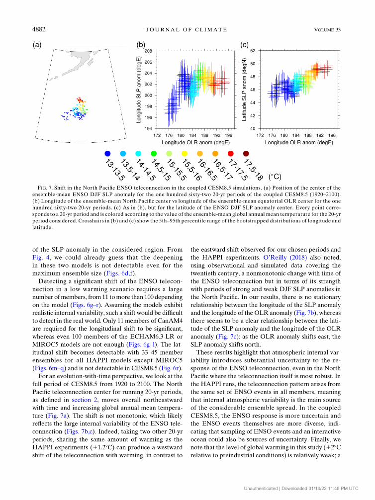
For an evolution-with-time perspective, we look at the

full period of CESM8.5 from 1920 to 2100. The North

Pacific teleconnection center for running 20-yr periods,

as defined in section 2, moves overall northeastward

with time and increasing global annual mean tempera-

ture (Fig. 7a). The shift is not monotonic, which likely

reflects the large internal variability of the ENSO tele-

connection (Figs. 7b,c). Indeed, taking two other 20-yr

periods, sharing the same amount of warming as the

HAPPI experiments (11.28C) can produce a westward

shift of the teleconnection with warming, in contrast to

the eastward shift observed for our chosen periods and

the HAPPI experiments. O’Reilly (2018) also noted,

using observational and simulated data covering the

twentieth century, a nonmonotonic change with time of

the ENSO teleconnection but in terms of its strength

with periods of strong and weak DJF SLP anomalies in

the North Pacific. In our results, there is no stationary

relationship between the longitude of the SLP anomaly

and the longitude of theOLR anomaly (Fig. 7b), whereas

there seems to be a clear relationship between the lati-

tude of the SLP anomaly and the longitude of the OLR

anomaly (Fig. 7c): as the OLR anomaly shifts east, the

SLP anomaly shifts north.

These results highlight that atmospheric internal var-

iability introduces substantial uncertainty to the re-

sponse of the ENSO teleconnection, even in the North

Pacific where the teleconnection itself is most robust. In

the HAPPI runs, the teleconnection pattern arises from

the same set of ENSO events in all members, meaning

that internal atmospheric variability is the main source

of the considerable ensemble spread. In the coupled

CESM8.5, the ENSO response is more uncertain and

the ENSO events themselves are more diverse, indi-

cating that sampling of ENSO events and an interactive

ocean could also be sources of uncertainty. Finally, we

note that the level of global warming in this study (128Crelative to preindustrial conditions) is relatively weak; a

FIG. 7. Shift in the North Pacific ENSO teleconnection in the coupled CESM8.5 simulations. (a) Position of the center of the

ensemble-mean ENSO DJF SLP anomaly for the one hundred sixty-two 20-yr periods of the coupled CESM8.5 (1920–2100).

(b) Longitude of the ensemble-mean North Pacific center vs longitude of the ensemble-mean equatorial OLR center for the one

hundred sixty-two 20-yr periods. (c) As in (b), but for the latitude of the ENSO DJF SLP anomaly center. Every point corre-

sponds to a 20-yr period and is colored according to the value of the ensemble-mean global annual mean temperature for the 20-yr

period considered. Crosshairs in (b) and (c) show the 5th–95th percentile range of the bootstrapped distributions of longitude and

latitude.

4882 JOURNAL OF CL IMATE VOLUME 33

Unauthenticated | Downloaded 01/14/22 11:45 PM UTC

larger global warming may reduce the number of events

required for a robust signal.

5. North American impacts

ENSO is an important source of predictability in

seasonal climate forecasts over North America (Shukla

et al. 2000). The North Pacific center of action is asso-

ciated with large-scale circulation anomalies that affect

temperature and rainfall over the continent (L’Heureux

et al. 2015). Given the response of the ENSO telecon-

nection to global warming in the HAPPI models, we ask

how ENSO’s impact over North America may be ex-

pected to change considering the role of internal vari-

ability and being aware that those changes will be more

likely to be true only if the equatorial SST zonal gradient

weakens with global warming. We only use the HAPPI

experiments in this section as they were purpose-

fully designed for impacts assessment under the Paris

Agreement targets.

a. Surface temperature impact

The present-day ENSO impact on near-surface air

temperature is relatively well simulated by the HAPPI

models, with warm anomalies over Alaska extending

southeast over Canada and the United States and cold

anomalies over the southern United States (Fig. 8a), in

agreement with observations (Fig. S7 and e.g., Ropelewski

andHalpert 1986; Livezey et al. 1997) and coupled climate

models (Deser et al. 2018; Perry et al. 2020).

The future impacts of ENSO over North America and

their robustness against internal variability and model

dependency strongly depend on the region considered.

Overall, the response of the temperature anomalies to

FIG. 8. Detection of the robust changes in DJF ENSO impacts over North America. (a) HAPPI ensemble-mean ENSO temperature

anomalies for the present-day experiment [interval: 0.4 K; zero-contour omitted; orange solid (blue dashed) lines represent positive

(negative) values] and (b) the response to 128C warming. (c),(d) As in (a) and (b), but for the precipitation anomalies [interval:

0.2mmday21; zero-contour omitted; green solid (brown dashed) lines represent positive (negative) values]. Vectors in (d) represent the

response of ENSO 850-hPa wind anomalies (m s21) to warming. (e) ENSO precipitation anomalies that arise from the thermodynamic

effect only [8.4% of present-day anomalies in (c)] [contour interval: 0.02mmday21; zero-contour omitted, solid (dashed) lines represent

positive (negative) values]. (f) Difference between (d) and (e), that is, the difference between the128C and the predicted [from Eq. (2)]

precipitation anomalies. Pink boxes in (a) and (b) show the regions in which the temperature and precipitation anomalies are averaged for

Fig. 9. The stippling is present when less than four models out of five agree on the sign of the HAPPI ensemble-mean response.

1 JUNE 2020 M I CHEL ET AL . 4883

Unauthenticated | Downloaded 01/14/22 11:45 PM UTC

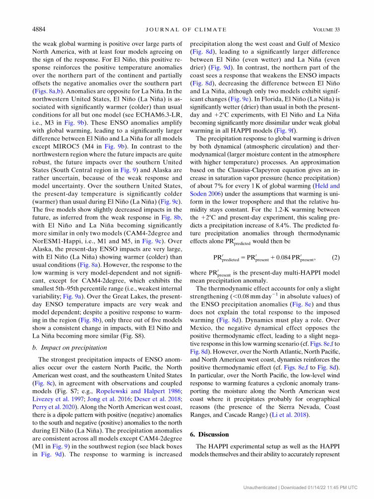
the weak global warming is positive over large parts of

North America, with at least four models agreeing on

the sign of the response. For El Niño, this positive re-

sponse reinforces the positive temperature anomalies

over the northern part of the continent and partially

offsets the negative anomalies over the southern part

(Figs. 8a,b). Anomalies are opposite for La Niña. In the

northwestern United States, El Niño (La Niña) is as-sociated with significantly warmer (colder) than usual

conditions for all but one model (see ECHAM6.3-LR,

i.e., M3 in Fig. 9b). These ENSO anomalies amplify

with global warming, leading to a significantly larger

difference between El Niño and La Niña for all models

except MIROC5 (M4 in Fig. 9b). In contrast to the

northwestern region where the future impacts are quite

robust, the future impacts over the southern United

States (South Central region in Fig. 9) and Alaska are

rather uncertain, because of the weak response and

model uncertainty. Over the southern United States,

the present-day temperature is significantly colder

(warmer) than usual during El Niño (La Niña) (Fig. 9c).The five models show slightly decreased impacts in the

future, as inferred from the weak response in Fig. 8b,

with El Niño and La Niña becoming significantly

more similar in only two models (CAM4-2degree and

NorESM1-Happi, i.e., M1 and M5, in Fig. 9c). Over

Alaska, the present-day ENSO impacts are very large,

with El Niño (La Niña) showing warmer (colder) than

usual conditions (Fig. 8a). However, the response to the

low warming is very model-dependent and not signifi-

cant, except for CAM4-2degree, which exhibits the

smallest 5th–95th percentile range (i.e., weakest internal

variability; Fig. 9a). Over the Great Lakes, the present-

day ENSO temperature impacts are very weak and

model dependent; despite a positive response to warm-

ing in the region (Fig. 8b), only three out of five models

show a consistent change in impacts, with El Niño and

La Niña becoming more similar (Fig. S8).

b. Impact on precipitation

The strongest precipitation impacts of ENSO anom-

alies occur over the eastern North Pacific, the North

American west coast, and the southeastern United States

(Fig. 8c), in agreement with observations and coupled

models (Fig. S7; e.g., Ropelewski and Halpert 1986;

Livezey et al. 1997; Jong et al. 2016; Deser et al. 2018;

Perry et al. 2020). Along theNorthAmerican west coast,

there is a dipole pattern with positive (negative) anomalies

to the south and negative (positive) anomalies to the north

during El Niño (La Niña). The precipitation anomalies

are consistent across all models except CAM4-2degree

(M1 in Fig. 9) in the southwest region (see black boxes

in Fig. 9d). The response to warming is increased

precipitation along the west coast and Gulf of Mexico

(Fig. 8d), leading to a significantly larger difference

between El Niño (even wetter) and La Niña (even

drier) (Fig. 9d). In contrast, the northern part of the

coast sees a response that weakens the ENSO impacts

(Fig. 8d), decreasing the difference between El Niñoand La Niña, although only two models exhibit signif-

icant changes (Fig. 9e). In Florida, El Niño (La Niña) issignificantly wetter (drier) than usual in both the present-

day and 128C experiments, with El Niño and La Niñabecoming significantly more dissimilar under weak global

warming in all HAPPI models (Fig. 9f).

The precipitation response to global warming is driven

by both dynamical (atmospheric circulation) and ther-

modynamical (larger moisture content in the atmosphere

with higher temperature) processes. An approximation

based on the Clausius-Clapeyron equation gives an in-

crease in saturation vapor pressure (hence precipitation)

of about 7% for every 1K of global warming (Held and

Soden 2006) under the assumptions that warming is uni-

form in the lower troposphere and that the relative hu-

midity stays constant. For the 1.2-K warming between

the 128C and present-day experiment, this scaling pre-

dicts a precipitation increase of 8.4%. The predicted fu-

ture precipitation anomalies through thermodynamic

effects alone PR0predicted would then be

PR0predicted 5PR0

present 1 0:084PR0present, (2)

where PR0present is the present-day multi-HAPPI model

mean precipitation anomaly.

The thermodynamic effect accounts for only a slight

strengthening (,0.08mmday21 in absolute values) of

the ENSO precipitation anomalies (Fig. 8e) and thus

does not explain the total response to the imposed

warming (Fig. 8d). Dynamics must play a role. Over

Mexico, the negative dynamical effect opposes the

positive thermodynamic effect, leading to a slight nega-

tive response in this lowwarming scenario (cf. Figs. 8e,f to

Fig. 8d). However, over theNorthAtlantic, North Pacific,

and North American west coast, dynamics reinforces the

positive thermodynamic effect (cf. Figs. 8e,f to Fig. 8d).

In particular, over the North Pacific, the low-level wind

response to warming features a cyclonic anomaly trans-

porting the moisture along the North American west

coast where it precipitates probably for orographical

reasons (the presence of the Sierra Nevada, Coast

Ranges, and Cascade Range) (Li et al. 2018).

6. Discussion

The HAPPI experimental setup as well as the HAPPI

models themselves and their ability to accurately represent

4884 JOURNAL OF CL IMATE VOLUME 33

Unauthenticated | Downloaded 01/14/22 11:45 PM UTC

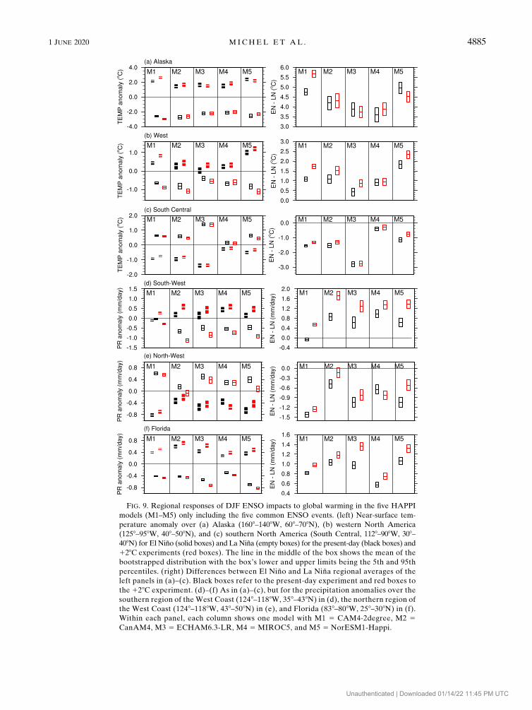
FIG. 9. Regional responses of DJF ENSO impacts to global warming in the five HAPPI

models (M1–M5) only including the five common ENSO events. (left) Near-surface tem-

perature anomaly over (a) Alaska (1608–1408W, 608–708N), (b) western North America

(1258–958W, 408–508N), and (c) southern North America (South Central, 1128–908W, 308–408N) for El Niño (solid boxes) and La Niña (empty boxes) for the present-day (black boxes) and

128C experiments (red boxes). The line in the middle of the box shows the mean of the

bootstrapped distribution with the box’s lower and upper limits being the 5th and 95th

percentiles. (right) Differences between El Niño and La Niña regional averages of the

left panels in (a)–(c). Black boxes refer to the present-day experiment and red boxes to

the 128C experiment. (d)–(f) As in (a)–(c), but for the precipitation anomalies over the

southern region of the West Coast (1248–1188W, 358–438N) in (d), the northern region of

the West Coast (1248–1188W, 438–508N) in (e), and Florida (838–808W, 258–308N) in (f).

Within each panel, each column shows one model with M1 5 CAM4-2degree, M2 5CanAM4, M3 5 ECHAM6.3-LR, M4 5 MIROC5, and M5 5 NorESM1-Happi.

1 JUNE 2020 M I CHEL ET AL . 4885

Unauthenticated | Downloaded 01/14/22 11:45 PM UTC

atmospheric processes are factors that can influence the

interpretation of the present study’s results, which features

an important role for internal variability in shaping future

changes of the ENSO teleconnection.

As the response of the ENSO teleconnection to global

warming is tightly linked to the response of convection

in the tropics, any uncertainty in the latter must be

considered in interpreting the results of this study. By

using the CMIP5 multimodel mean SST response, the

HAPPI setup assumes that the zonal SST gradient in

the equatorial Pacific will weaken in the future, fa-

voring an eastward migration of convection. However,

recent studies have argued that the real world may not

be trending toward a warmer eastern equatorial Pacific

in the same way that the models are (L’Heureux et al.

2013; Sohn et al. 2013; Sandeep et al. 2014; Coats and

Karnauskas 2017; Bayr et al. 2019; Johnson et al. 2019;

Seager et al. 2019). If this is correct, the ENSO tele-

connection may not shift eastward with global warming,

although even uniform tropical warming does seem to

create some eastward shift (Zhou et al. 2014). Whether

models are indeed incorrect in this regard is an active

topic of research. In addition to shifting, the convection

anomalies associated with ENSO are also expected to

strengthen with global warming (Kug et al. 2010; Seager

et al. 2012; Johnson et al. 2019), which can then influence

the ENSO teleconnection through the SLP anomaly

strength, for example. Idealized simulations with pre-

scribed equatorial convection could be useful in inves-

tigating the relative roles of the position and strength of

the convection anomalies in the North Pacific ENSO

teleconnection.

The results from the uncoupled HAPPI models are

in relatively good agreement with those of the coupled

CESM1 model and in qualitative agreement with most

of the CMIP5 models in a stronger warming scenario

(Christensen et al. 2013). However, the similarities be-

tween HAPPI, CESM8.5, and CMIP5 are corroborated

by Deser et al.’s (2017) study, which does not show large

differences in the present-day ENSO teleconnection

in pacemaker versus Tropical Ocean and the Global

Atmosphere (TOGA) simulations. We do not have

the appropriate experiments to test quantitatively

whether this is true for the response to warming, but

the similarity between HAPPI and CESM8.5 suggests

the results would be similar in coupled frameworks.

This is despite the fact that the HAPPI framework

does not represent the two-way atmosphere–ocean

interactions, including changes in upwelling, ther-

mocline depth, and surface heat and radiative fluxes

that can modify the amplitude, pattern, and vari-

ability of ENSO (Collins et al. 2010). It would be

worthwhile confirming these results with a wider

range of coupled large ensembles where the ocean

can react to atmospheric changes (Garfinkel et al.

2018), the nature of ENSO can also change under

warming, and the simulations can capture a richer

spectrum of ENSO events. In addition, there may be

other sources of variability that are missing from this

HAPPI ensemble that may further enhance the un-

certainty in projected changes. For example, the

Pacific decadal oscillation (PDO) does not play an

important role over the short HAPPI record, but it

could further increase the sampling uncertainty if

it were present, or if the PDO and/or its modulation

of ENSO were to change with global warming too

(Zhang and Delworth 2016; Mantua et al. 1997;

Zhang et al. 1997; Wang and An 2001; Jia and Ge

2017; Wills et al. 2018, and references therein).

ENSO is known to modulate the NAO with El Niño(La Niña) favoring the negative (positive) phase of

the NAO (e.g., Fraedrich and Müller 1992). One of

the pathways connecting ENSO to the North Atlantic

is through the stratosphere (Jiménez-Esteve andDomeisen

2018). However, the HAPPI models do not resolve the

stratosphere very well and thus may not adequately

represent troposphere–stratosphere interactions, which

may impact the response to warming of the ENSO in-

fluence onto the NAO.

Our overall aim was to assess the uncertainty due to

atmospheric internal variability in the response of the

extratropical ENSO teleconnection to warming by tak-

ing advantage of a very large ensemble of simulations.

There are important caveats concerning experiment

design and model uncertainty, as discussed above.

However, the results are robust and emphasize the im-

portance of sampling the internal variability thoroughly

in order to accurately determine the forced response

under a low warming scenario, as would be expected in

the coming decades if the Paris Agreement target is met.

7. Conclusions

The wintertime atmospheric teleconnection of ENSO

in the North Pacific shifts northeastward by a few de-

grees with 128C of global warming in the HAPPI large

ensemble. The shift is tightly linked to changes in the

position and intensity of the forcing by convection in the

equatorial region, as represented by OLR: the farther

east and the stronger (more negative) the tropical OLR

anomaly, the farther northeast the extratropical SLP

anomaly. The displacement relationship has been noted

in other climatemodels, with relevance for issues such as

impacts of cold tongue SST biases, which are common to

many models (e.g., Bayr et al. 2019). Detecting the

northeastward shift in the SLP anomaly requires at least

4886 JOURNAL OF CL IMATE VOLUME 33

Unauthenticated | Downloaded 01/14/22 11:45 PM UTC

10–15 HAPPI ensemble members of 1 decade each, or

equivalently 50–75 ENSO events, in both the present

and future climates. Some models (MIROC5, and to a

lesser extent, ECHAM6.3-LR) show a tendency toward

a northeastward shift, but the shift is not significant even

with 100 ensemble members (500 ENSO events). Even

more eventsmay be needed if one includes other sources

of uncertainty not considered in our experimental setup,

such as changes in ENSO itself (Berner et al. 2020).

CESM8.5, which includes eventual changes in ENSO

under a weak warming, also shows a tendency toward a

northeastward shift that is not significant with 40 mem-

bers. However, fewer members would be required if the

signal were greater (e.g., under a higher global warming

scenario). The results highlight that, for low warming

scenarios, changes in the atmospheric ENSO telecon-

nection are highly uncertain due to internal atmospheric

variability. This large uncertainty may explain why past

studies using smaller ensemble sizes have found differ-

ent ENSO responses to climate change (e.g., Meehl and

Teng 2007; Schneider et al. 2009; Christensen et al.

2013). It also suggests that the observational period

(1920–2013), which includes 32 ENSO events (Deser

et al. 2017, 2018), is too short to use as a baseline for

assessing changes in the ENSO teleconnection under

Paris Agreement warming targets. For North American

impacts, precipitation changes with global warming

are relatively robust compared to temperature changes

and are dominated by the changes in the atmospheric

circulation rather than the thermodynamic effect.

Acknowledgments. The authors thank the three re-

viewers whose comments improved themanuscript. This

work was funded by the Norwegian Research Council

projects 255027 DynAMiTe, 231716 jetSTREAM, and

261821 HappiEVA. We are thankful to UNINETT

Sigma2 AS for managing the national infrastructure

for computational science in Norway (project NS9082K),

the European Centre for Medium-Range Weather

Forecasts for providing the ERA-Interim reanalyses,

the HAPPI project for producing such a very large

ensemble of simulations, and the National Center for

Atmospheric Research for providing the large en-

semble of the Community Earth System Model.

REFERENCES

Atwood, A. R., D. S. Battisti, A. T. Wittenberg, W. H. G. Roberts,

and D. J. Vimont, 2017: Characterizing unforced multi-

decadal variability of ENSO: A case study with the GFDL

CM2.1 coupled GCM. Climate Dyn., 49, 2845–2862, https://

doi.org/10.1007/s00382-016-3477-9.

Bayr, T., D. I. V. Domeisen, and C.Wengel, 2019: The effect of the

equatorial Pacific cold SST bias on simulated ENSO tele-

connections to the North Pacific and California.Climate Dyn.,

53, 3771–3789, https://doi.org/10.1007/s00382-019-04746-9.

Berner, J., H. M. Christensen, and P. D. Sardeshmukh, 2020: Does

ENSO regularity increase in a warming climate? J. Climate,

33, 1247–1259, https://doi.org/10.1175/JCLI-D-19-0545.1.

Bjerknes, J., 1969: Atmospheric teleconnections from the equa-

torial Pacific. Mon. Wea. Rev., 97, 163–172, https://doi.org/

10.1175/1520-0493(1969)097,0163:ATFTEP.2.3.CO;2.

Brands, S., 2017: Which ENSO teleconnections are robust to in-

ternal atmospheric variability? Geophys. Res. Lett., 44, 1483–

1493, https://doi.org/10.1002/2016GL071529.

Brönnimann, S., 2007: Impact of El Niño–Southern Oscillation on

European climate.Rev.Geophys., 45, RG3003, https://doi.org/

10.1029/2006RG000199.

Cai, W., P. van Rensch, T. Cowan, and H. H. Hendon, 2011:

Teleconnection pathways of ENSO and the IOD and the

mechanisms for impacts on Australian rainfall. J. Climate, 24,

3910–3923, https://doi.org/10.1175/2011JCLI4129.1.

——, and Coauthors, 2015: ENSO and greenhouse warming. Nat.

ClimateChange, 5, 849–859, https://doi.org/10.1038/nclimate2743.

Chen, M., and A. Kumar, 2015: Influence of ENSO SSTs on the

spread of the probability density function for precipitation and

land surface temperature. Climate Dyn., 45, 965–974, https://

doi.org/10.1007/s00382-014-2336-9.

Christensen, J. H., and Coauthors, 2013: Climate phenomena and

their relevance for future regional climate change. Climate

Change 2013: The Physical Science Basis, T. F. Stocker et al.,

Eds., Cambridge University Press, 1217–1308.

Coats, S., and K. B. Karnauskas, 2017: Are simulated and observed

twentieth century tropical Pacific sea surface temperature

trends significant relative to internal variability? Geophys. Res.

Lett., 44, 9928–9937, https://doi.org/10.1002/2017GL074622.

Collins, M., and Coauthors, 2010: The impact of global warming on

the tropical Pacific Ocean and El Niño. Nat. Geosci., 3, 391–

397, https://doi.org/10.1038/ngeo868.

Dee, D. P., and Coauthors, 2011: The ERA-Interim reanalysis:

Configuration and performance of the data assimilation sys-

tem.Quart. J. Roy. Meteor. Soc., 137, 553–597, https://doi.org/

10.1002/qj.828.

Deser, C., I. R. Simpson, K. A. McKinnon, and A. S. Phillips, 2017:

The Northern Hemisphere extratropical atmospheric circu-

lation response to ENSO:How well do we know it and how do

we evaluate models accordingly? J. Climate, 30, 5059–5082,

https://doi.org/10.1175/JCLI-D-16-0844.1.

——, ——, A. S. Phillips, and K. A. McKinnon, 2018: How well do

we know ENSO’s climate impacts over North America, and

how do we evaluate models accordingly? J. Climate, 31, 4991–

5014, https://doi.org/10.1175/JCLI-D-17-0783.1.

Diaz, H. F., M. P. Hoerling, and J. K. Eischeid, 2001: ENSO vari-

ability, teleconnections and climate change. Int. J. Climatol.,

21, 1845–1862, https://doi.org/10.1002/joc.631.Drouard, M., and C. Cassou, 2019: Amodeling and process-oriented

study to investigate the projected change of ENSO-forced

wintertime teleconnectivity in a warmer world. J. Climate, 32,

8047–8068, https://doi.org/10.1175/JCLI-D-18-0803.1.

Fasullo, J., B. L. Otto-Bliesner, and S. Stevenson, 2018: ENSO’s

changing influence on temperature, precipitation, and wildfire

in a warming climate. Geophys. Res. Lett., 45, 9216–9225,

https://doi.org/10.1029/2018GL079022.

Feng, J., W. Chen, and Y. Li, 2017: Asymmetry of the winter extra-

tropical teleconnections in the Northern Hemisphere associ-

ated with two types of ENSO. Climate Dyn., 48, 2135–2151,

https://doi.org/10.1007/s00382-016-3196-2.

1 JUNE 2020 M I CHEL ET AL . 4887

Unauthenticated | Downloaded 01/14/22 11:45 PM UTC

——, T. Lian, J. Ying, J. Li, and G. Li, 2020: Do CMIP5 models

show El Niño diversity? J. Climate, 33, 1619–1641, https://

doi.org/10.1175/JCLI-D-18-0854.1.

Fraedrich, K., 1994: An ENSO impact on Europe? Tellus, 46A,

541–552, https://doi.org/10.3402/tellusa.v46i4.15643.

——, and K.Müller, 1992: Climate anomalies in Europe associated

with ENSO extremes. Int. J. Climatol., 12, 25–31, https://

doi.org/10.1002/joc.3370120104.

Garfinkel, C. I., I. Weinberger, I. P. White, L. D. Oman, V. Aquila,

and Y.-K. Lim, 2018: The salience of nonlinearities in the

boreal winter response to ENSO: North Pacific and North

America.ClimateDyn., 52, 4429–4446, https://doi.org/10.1007/

s00382-018-4386-x.

Grimm, A. M., and R. G. Tedeschi, 2009: ENSO and extreme

rainfall events in South America. J. Climate, 22, 1589–1609,

https://doi.org/10.1175/2008JCLI2429.1.

Held, I. M., and B. J. Soden, 2006: Robust responses of the hy-

drological cycle to global warming. J. Climate, 19, 5686–5699,

https://doi.org/10.1175/JCLI3990.1.

Herceg Bulic, I., and �C. Brankovic, 2007: ENSO forcing of

the Northern Hemisphere climate in a large ensemble

of model simulations based on a very long SST record.

Climate Dyn., 28, 231–254, https://doi.org/10.1007/s00382-

006-0181-1.

——, ——, and F. Kucharski, 2012: Winter ENSO teleconnections

in a warmer climate. Climate Dyn., 38, 1593–1613, https://

doi.org/10.1007/s00382-010-0987-8.

Hoerling, M. P., and M. Ting, 1994: Organization of extratropical

transients during El Niño. J. Climate, 7, 745–766, https://doi.org/

10.1175/1520-0442(1994)007,0745:OOETDE.2.0.CO;2.

——, A. Kumar, and M. Zhong, 1997: El Niño, La Niña, and the

nonlinearity of their teleconnections. J. Climate, 10, 1769–1786,

https://doi.org/10.1175/1520-0442(1997)010,1769:ENOLNA.2.0.CO;2.

Horel, J. D., and J. M. Wallace, 1981: Planetary-scale atmospheric

phenomena associated with the Southern Oscillation.Mon. Wea.

Rev., 109, 813–829, https://doi.org/10.1175/1520-0493(1981)

109,0813:PSAPAW.2.0.CO;2.

Huang, R., and Y. Wu, 1989: The influence of ENSO on the sum-

mer climate change in China and its mechanism. Adv. Atmos.

Sci., 6, 21–32, https://doi.org/10.1007/BF02656915.Jia, X., and J. Ge, 2017: Modulation of the PDO to the relationship

between moderate ENSO events and the winter climate over

North America. Int. J. Climatol., 37, 4275–4287, https://

doi.org/10.1002/joc.5083.

Jiménez-Esteve, B., andD. I. V. Domeisen, 2018: The tropospheric

pathway of the ENSO–North Atlantic teleconnection.

J. Climate, 31, 4563–4584, https://doi.org/10.1175/JCLI-D-

17-0716.1.

——, and——, 2019: Nonlinearity in theNorth Pacific atmospheric

response to a linear ENSO forcing. Geophys. Res. Lett., 46,

2271–2281, https://doi.org/10.1029/2018GL081226.

Johnson, N. C.,M. L. L’Heureux, C.-H. Chang, and Z.-Z.Hu, 2019:

On the delayed coupling between ocean and atmosphere in

recent weak El Niño episodes.Geophys. Res. Lett., 46, 11 416–

11 425, https://doi.org/10.1029/2019GL084021.

Jong, B.-T., M. Ting, and R. Seager, 2016: El Niño’s impact on

California precipitation: Seasonality, regionality, and El Niñointensity. Quart. J. Roy. Meteor. Soc., 11, 054021, https://

doi.org/10.1088/1748-9326/11/5/054021.

Kay, J. E., and Coauthors, 2015: The Community Earth System

Model (CESM) large ensemble project: A community re-

source for studying climate change in the presence of internal

climate variability. Bull. Amer. Meteor. Soc., 96, 1333–1349,

https://doi.org/10.1175/BAMS-D-13-00255.1.

Kug, J.-S., S.-I. An, Y.-G. Ham, and I.-S. Kang, 2010: Changes in

El Niño and La Niña teleconnections over North Pacific–

America in the global warming simulations. Theor. Appl.

Climatol., 100, 275–282, https://doi.org/10.1007/s00704-009-

0183-0.

L’Heureux, M. L., S. Lee, and B. Lyon, 2013: Recent multidecadal

strengthening of the Walker circulation across the tropical

Pacific. Nat. Climate Change, 3, 571–576, https://doi.org/

10.1038/nclimate1840.

——, M. K. Tippett, and A. G. Barnston, 2015: Characterizing

ENSO coupled variability and its impact on North American

seasonal precipitation and temperature. J. Climate, 28, 4231–

4245, https://doi.org/10.1175/JCLI-D-14-00508.1.

Li, C., and Coauthors, 2018: Midlatitude atmospheric circulation

responses under 1.5 and 2.08C warming and implications for

regional impacts. Earth Syst. Dyn., 9, 359–382, https://doi.org/

10.5194/esd-9-359-2018.

Liu, Z., S. Vavrus, F. He, N. Wen, and Y. Zhong, 2005: Rethinking

tropical ocean response to global warming: The enhanced

equatorial warming. J. Climate, 18, 4684–4700, https://doi.org/

10.1175/JCLI3579.1.

Livezey, R. E., M. Masutani, A. Leetmaa, H. Rui, M. Ji, and

A.Kumar, 1997: Teleconnective response of the Pacific–North

American region atmosphere to large central equatorial Pacific

SST anomalies. J. Climate, 10, 1787–1820, https://doi.org/10.1175/

1520-0442(1997)010,1787:TROTPN.2.0.CO;2.

Mantua, N. J., S. R. Hare, Y. Zhang, J. M. Wallace, and R. C.

Francis, 1997: A Pacific interdecadal climate oscillation with

impacts on salmon production. Bull. Amer. Meteor. Soc., 78,

1069–1079, https://doi.org/10.1175/1520-0477(1997)078,1069:

APICOW.2.0.CO;2.

Meehl, G. A., and H. Teng, 2007: Multi-model changes in El Niñoteleconnections over North America in a future warmer

climate. Climate Dyn. 29, 779–790, https://doi.org/10.1007/

S00382-007-0268-3.

Mitchell, D., R. James, P. M. Forster, R. A. Betts, H. Shiogama,

and M. Allen, 2016: Realizing the impacts of a 1.58C warmer

world. Nat. Climate Change, 6, 735–737, https://doi.org/10.1038/

nclimate3055.

——, and Coauthors, 2017: Half a degree additional warming,

prognosis and projected impacts (HAPPI): Background and

experimental design.Geosci. Model Dev., 10, 571–583, https://

doi.org/10.5194/gmd-10-571-2017.

Müller, W. A., and E. Roeckner, 2006: ENSO impact on midlati-

tude circulation patterns in future climate change projections.

Geophys. Res. Lett., 33, L05711, https://doi.org/10.1029/

2005GL025032.

——, and ——, 2008: ENSO teleconnections in projections of

future climate in ECHAM5/MPI-OM. Climate Dyn., 31,

533–549, https://doi.org/10.1007/s00382-007-0357-3.

Okumura,Y.M., andC.Deser, 2010: Asymmetry in the duration of

El Niño andLaNiña. J. Climate, 23, 5826–5843, https://doi.org/

10.1175/2010JCLI3592.1.

Olonscheck, D., and D. Notz, 2017: Consistently estimating internal

climate variability from climate model simulations. J. Climate,

30, 9555–9573, https://doi.org/10.1175/JCLI-D-16-0428.1.

O’Reilly, C., 2018: Interdecadal variability of the ENSO telecon-

nection to the wintertime North Pacific. Climate Dyn., 51,

3333–3350, https://doi.org/10.1007/s00382-018-4081-y.

Perry, S. J., S. McGregor, A. Sen Gupta, M. H. England, and

N. Maher, 2020: Projected late 21st century changes to the

4888 JOURNAL OF CL IMATE VOLUME 33

Unauthenticated | Downloaded 01/14/22 11:45 PM UTC

regional impacts of the El Niño–SouthernOscillation.Climate

Dyn., 54, 395–412, https://doi.org/10.1007/s00382-019-05006-6.

Plisnier, P. D., S. Serneels, and E. F. Lambin, 2000: Impact of

ENSOonEastAfrican ecosystems:Amultivariate analysis based

on climate and remote sensing data. Global Ecol. Biogeogr., 9,

481–497, https://doi.org/10.1046/j.1365-2699.2000.00208.x.

Ropelewski, C. F., and M. S. Halpert, 1986: North American

precipitation and temperature patterns associated with the

El Niño/Southern Oscillation (ENSO). Mon. Wea. Rev.,

114, 2352–2362, https://doi.org/10.1175/1520-0493(1986)114,2352:

NAPATP.2.0.CO;2.

——, and ——, 1987: Global and regional scale precipitation

patterns associated with the El Niño/Southern Oscillation.

Mon. Wea. Rev., 115, 1606–1626, https://doi.org/10.1175/

1520-0493(1987)115,1606:GARSPP.2.0.CO;2.

Sandeep, S., F. Stordal, P. D. Sardeshmukh, and G. P. Compo,

2014: Pacific Walker circulation variability in coupled and

uncoupled climate models. Climate Dyn., 43, 103–117, https://

doi.org/10.1007/s00382-014-2135-3.

Schneider, E. K., M. J. Fennessy, and J. L. Kinter III, 2009: A

statistical-dynamical estimate of winter ENSO teleconnections

in a future climate. J. Climate, 22, 6624–6638, https://doi.org/

10.1175/2009JCLI3147.1.

Seager, R., N. Naik, andL.Vogel, 2012:Does global warming cause

intensified interannual hydroclimate variability? J. Climate,

25, 3355–3372, https://doi.org/10.1175/JCLI-D-11-00363.1.

——, M. Cane, N. Henderson, D.-E. Lee, R. Abernathey, and

H. Zhang, 2019: Strengthening tropical Pacific zonal sea sur-

face temperature gradient consistent with rising greenhouse

gases. Nat. Climate Change, 9, 517–522, https://doi.org/10.1038/s41558-019-0505-x.

Shukla, J., and Coauthors, 2000: Dynamical seasonal prediction.

Bull. Amer. Meteor. Soc., 81, 2593–2606, https://doi.org/

10.1175/1520-0477(2000)081,2593:DSP.2.3.CO;2.

Sohn, B. J., S.-W. Yeh, J. Schmetz, and H.-J. Song, 2013:

Observational evidences of Walker circulation change over

the last 30 years contrasting with GCM results. Climate Dyn.,

40, 1721–1732, https://doi.org/10.1007/s00382-012-1484-z.

Stevenson, S., B. Fox-Kemper,M. Jochum,R. Neale, C. Deser, and

G.Meehl, 2012:Will there be a significant change to ElNiño inthe twenty-first century? J. Climate, 25, 2129–2145, https://doi.org/10.1175/JCLI-D-11-00252.1.

——, 2012: Significant changes to ENSO strength and impacts in

the twenty-first century: Results from CMIP5. Geophys. Res.

Lett., 39, L17703, https://doi.org/10.1029/2012GL052759.

Toniazzo, T., and A. A. Scaife, 2006: The influence of ENSO on

winter North Atlantic climate.Geophys. Res. Lett., 33, L24704,

https://doi.org/10.1029/2006GL027881.

UN-FCCC, 2015: Adoption of the Paris Agreement, Conference of

the Parties, 2015. United Nations Framework Convention on

Climate Change, https://unfccc.int/resource/docs/2015/cop21/

eng/l09r01.pdf.

Vecchi, G. A., and B. J. Soden, 2007: Global warming and the

weakening of the tropical circulation. J. Climate, 20, 4316–4340, https://doi.org/10.1175/JCLI4258.1.

——, ——, A. T. Wittenberg, I. M. Held, A. Leetmaa, and M. J.

Harrison, 2006: Weakening of tropical Pacific atmospheric

circulation due to anthropogenic forcing. Nature, 441, 73–76,https://doi.org/10.1038/nature04744.

Wallace, J. M., and D. S. Gutzler, 1981: Teleconnections in the

geopotential height field during the Northern Hemisphere.

Mon. Wea. Rev., 109, 784–812, https://doi.org/10.1175/1520-0493(1981)109,0784:TITGHF.2.0.CO;2.

Wang, B., and S.-I. An, 2001: Why the properties of El Niñochanged during the late 1970s. Geophys. Res. Lett., 28, 3709–3712, https://doi.org/10.1029/2001GL012862.

Wills, R. C., T. Schneider, J. M. Wallace, D. S. Battisti, and D. L.

Hartmann, 2018: Disentangling global warming, multidecadal

variability, and El Niño in Pacific temperatures.Geophys. Res.

Lett., 45, 2487–2496, https://doi.org/10.1002/2017GL076327.

Zhang, L., and T. L. Delworth, 2016: Simulated response of the

Pacific decadal oscillation to climate change. J. Climate, 29,

5999–6018, https://doi.org/10.1175/JCLI-D-15-0690.1.

Zhang, T., X. Shao, and S. Li, 2017: Impacts of atmospheric pro-

cesses on ENSO asymmetry: A comparison between CESM1

andCCSM4. J. Climate, 30, 9743–9762, https://doi.org/10.1175/JCLI-D-17-0360.1.

Zhang, W., Z. Wang, M. F. Stuecker, A. G. Turner, F.-F. Jin, and

X. Geng, 2019: Impact of ENSO longitudinal position on tel-

econnections to the NAO. Climate Dyn., 52, 257–274, https://doi.org/10.1007/s00382-018-4135-1.

Zhang, Y., J. M. Wallace, and D. S. Battisti, 1997: ENSO-like in-

terdecadal variability: 1990–93. J. Climate, 10, 1004–1020,

https://doi.org/10.1175/1520-0442(1997)010,1004:ELIV.2.0.CO;2.

Zheng, X.-T., S.-P. Xie, L.-H. Lv, and Z.-Q. Zhou, 2016:

Intermodel uncertainty in ENSO amplitude change tied to

Pacific Ocean warming pattern. J. Climate, 29, 7265–7279,

https://doi.org/10.1175/JCLI-D-16-0039.1.

——, C. Hui, and S.-W. Yeh, 2018: Response of ENSO amplitude

to global warming in CESM large ensemble: Uncertainty due

to internal variability. Climate Dyn., 50, 4019–4035, https://

doi.org/10.1007/s00382-017-3859-7.

Zhou, Z.-Q., S.-P. Xie, X.-T. Zheng, Q. Liu, and H. Wang, 2014:

Global warming-induced changes in El Niño teleconnections

over the North Pacific and North America. J. Climate, 27,

9050–9064, https://doi.org/10.1175/JCLI-D-14-00254.1.

Zhu, X., andZ. Liu, 2009: Tropical SST response to global warming

in the twentieth century. J. Climate, 22, 1305–1312, https://doi.org/10.1175/2008JCLI2164.1.

1 JUNE 2020 M I CHEL ET AL . 4889

Unauthenticated | Downloaded 01/14/22 11:45 PM UTC