The physics of climate variability and climate change - CentAUR

The physics of climate variability and climate change Article

Published Version

Ghil, M. and Lucarini, V. ORCID: https://orcid.org/0000-0001-9392-1471 (2020) The physics of climate variability and climate change. Reviews of Modern Physics, 92 (3). 035002. ISSN 0034-6861 doi: https://doi.org/10.1103/RevModPhys.92.035002 Available at https://centaur.reading.ac.uk/91299/

It is advisable to refer to the publisher’s version if you intend to cite from the work. See Guidance on citing .

To link to this article DOI: http://dx.doi.org/10.1103/RevModPhys.92.035002

Publisher: American Physical Society

All outputs in CentAUR are protected by Intellectual Property Rights law, including copyright law. Copyright and IPR is retained by the creators or other copyright holders. Terms and conditions for use of this material are defined in the End User Agreement .

www.reading.ac.uk/centaur

CentAUR

Central Archive at the University of Reading

http://centaur.reading.ac.uk/71187/10/CentAUR%20citing%20guide.pdf

http://www.reading.ac.uk/centaur

http://centaur.reading.ac.uk/licence

Reading’s research outputs online

The physics of climate variability and climate change

Michael Ghil

Geosciences Department and Laboratoire de Meteorologie Dynamique (CNRS and IPSL),Ecole Normale Superieure and PSL University, F-75231 Paris Cedex 05, Franceand Department of Atmospheric and Oceanic Sciences, University of California,Los Angeles, California 90095-1565, USA

Valerio Lucarini

Department of Mathematics and Statistics, University of Reading,Reading RG66AX, United Kingdom,Centre for the Mathematics of Planet Earth, University of Reading,Reading RG66AX, United Kingdom,and CEN—Institute of Meteorology, University of Hamburg, Hamburg 20144, Germany

(published 31 July 2020)

The climate is a forced, dissipative, nonlinear, complex, and heterogeneous system that is out ofthermodynamic equilibrium. The system exhibits natural variability on many scales of motion, in timeas well as space, and it is subject to various external forcings, natural as well as anthropogenic. Thisreview covers the observational evidence on climate phenomena and the governing equations ofplanetary-scale flow and presents the key concept of a hierarchy of models for use in the climatesciences. Recent advances in the application of dynamical systems theory, on the one hand, andnonequilibrium statistical physics, on the other hand, are brought together for the first time and shownto complement each other in helping understand and predict the system’s behavior. Thesecomplementary points of view permit a self-consistent handling of subgrid-scale phenomena asstochastic processes, as well as a unified handling of natural climate variability and forced climatechange, along with a treatment of the crucial issues of climate sensitivity, response, and predictability.

DOI: 10.1103/RevModPhys.92.035002

CONTENTS

I. Introduction and Motivation 2A. Basic facts of the climate sciences 2B. More than “just” science 4

1. The Intergovernmental Panel on Climate Change 42. Hockey stick controversy and climate blogs 5

C. This review 5II. Introduction to Climate Dynamics 7

A. Climate observations: Direct and indirect 71. Instrumental data and reanalyses 72. Proxy data 10

B. Climate variability on multiple Timescales 111. A survey of climatic timescales 122. Atmospheric variability in mid-latitudes 13

C. Basic properties and fundamental equations 161. Governing equations 162. Approximate balances and filtering 17

a. Hydrostatic balance 17b. Geostrophic balance 18

3. Quasigeostrophy and weather forecasting 19D. Climate prediction and climate model performance 20

1. Predicting the state of the system 222. Predicting the system’s statistical properties 233. Metrics for model validation 24

III. Climate Variability and the Modeling Hierarchy 25A. Radiation balance and energy balance models 25B. Other atmospheric processes and models 28C. Oscillations in the ocean’s thermohaline circulation 28

1. Theory and simple models 28

2. Bifurcation diagrams for GCMs 29D. Bistability, oscillations, and bifurcations 31

1. Bistability and steady-state bifurcations 312. Oscillatory instabilities and Hopf bifurcations 32

E. Main modes of variability 331. Modes of variability and extended-range

prediction 332. Coupled atmosphere-ocean modes of

variability 343. Atmospheric low-frequency variability 34

F. Internal variability and routes to chaos 361. A simple model of the double-gyre circulation 372. Bifurcations in the double-gyre problem 38

a. Symmetry-breaking bifurcation 38b. Gyre modes 38c. Global bifurcations 39

G. Multiple scales: Stochastic and memory effects 401. Fast scales and their deterministic

parametrization 402. An example: Convective parametrization 413. Stochastic parametrizations 414. Modeling memory effects 42

a. The Mori-Zwanzig formalism 43b. EMR methodology 43c. Role of memory effects in EMR 43d. EMR applications 44e. Explicit derivation of the parametrized

equations 45IV. Climate Sensitivity and Response 46

A. A simple framework for climate sensitivity 46

REVIEWS OF MODERN PHYSICS, VOLUME 92, JULY–SEPTEMBER 2020

0034-6861=2020=92(3)=035002(77) 035002-1 © 2020 American Physical Society

https://orcid.org/0000-0001-5177-7133

https://orcid.org/0000-0001-9392-1471

https://crossmark.crossref.org/dialog/?doi=10.1103/RevModPhys.92.035002&domain=pdf&date_stamp=2020-07-31

https://doi.org/10.1103/RevModPhys.92.035002




B. Climate sensitivity: Uncertainties and ambiguities 47C. Transient climate response (TCR) 48D. Beyond climate sensitivity 49E. A general framework for climate response 50

1. Pullback attractors (PBAs) 502. Fluctuation dissipation and climate change 513. Ruelle response theory 514. Climate change prediction via Ruelle

response theory 535. Slow correlation decay and sensitive

parameter dependence 54V. Critical Transitions and Edge States 56

A. Bistability for gradient flows and EBMs 56B. Finding the edge states 58C. Invariant measures and noise-induced transitions 59D. Nearing critical transitions 60E. Chaos-to-chaos transition 60

VI. Conclusions 62List of Symbols and Abbreviations 64Acknowledgments 64References 65

I. INTRODUCTION AND MOTIVATION

A. Basic facts of the climate sciences

The climate system is forced, dissipative, chaotic, and outof equilibrium; its complex natural variability arises from theinterplay of positive and negative feedbacks, instabilities, andsaturation mechanisms. These processes span a broad range ofspatial and temporal scales and include many chemical speciesand all of the most common physical phases. The system’sheterogeneous phenomenology includes the mycrophysics ofclouds, cloud-radiation interactions, atmospheric and oceanicboundary layers, and several scales of turbulence (Ghil, 2019);it evolves, furthermore, under the action of large-scale agentsthat drive and modulate its evolution, mainly differential solarheating and the Earth’s rotation and gravitation.As is often the case, the complexity of the physics is

interwoven with the chaotic character of the dynamics.Moreover, the climate system’s large natural variability ondifferent timescales is strongly affected by relatively smallchanges in the forcing, anthropogenic as well as natural (Ghiland Childress, 1987; Peixoto and Oort, 1992; Lucarini,Blender et al., 2014).On the macroscopic level, climate is driven by differences

in the absorption of solar radiation throughout the depth of theatmosphere, as well as in a narrow surface layer of the oceanand of the soil; the system’s actual governing equations aregiven in Sec. II.C. The prevalence of absorption at the surfaceand in the atmosphere’s lower levels leads through severalprocesses to compensating vertical energy fluxes, mostnotably, fluxes of infrared radiation throughout the atmos-phere and convective motions in the troposphere; see Fig. 1.More solar radiation is absorbed in the low latitudes,

leading to horizontal energy fluxes as well. The atmosphere’slarge-scale circulation is to first order a result of thesehorizontal and vertical fluxes arising from the gradients insolar radiation absorption, in which the hydrological cycleplays a key role as well. The ocean circulation, in turn, is setinto motion by surface or near-surface exchanges of mass,

momentum, and energy with the atmosphere: the so-calledwind-driven component of the circulation is due mainly to thewind stress and the thermohaline one is due mainly tobuoyancy fluxes (Dijkstra, 2005; Dijkstra and Ghil, 2005;Kuhlbrodt et al., 2007). The coupled atmospheric and oceaniccirculation reduces the temperature differences between thetropics and polar regions with respect to that on an otherwisesimilar planet with no horizontal energy transfers (Lorenz,1967; Peixoto and Oort, 1992; Held, 2001; Lucarini andRagone, 2011). At steady state, the convergence of enthalpytransported by the atmosphere and the ocean compensatesfor the radiative imbalance at the top of the atmosphere;see Fig. 2.The classical theory of the general circulation of the

atmosphere (Lorenz, 1967) describes in further detail howthe mechanisms of energy generation, conversion, and dis-sipation produce the observed circulation, which deviatessubstantially from the highly idealized, zonally symmetricpicture sketched so far. According to Lorenz (1955), atmos-pheric large-scale flows result from the conversion of availablepotential energy, which is produced by the atmosphere’sdifferential heating, into kinetic energy, and the Lorenz(1967) energy cycle is completed by energy cascading tosmaller scales to eventually be dissipated. McWilliams (2019)provided an up-to-date criticism of and further perspective onthis theory.Overall, the climate system can be seen as a thermal engine

capable of transforming radiative heat into mechanical energywith a given, highly suboptimal efficiency given the manyirreversible processes that make it less than ideal (Pauluis andHeld, 2002; Kleidon and Lorenz, 2005; Lucarini, 2009b;Lucarini, Blender et al., 2014). This conversion occursthrough genuinely three-dimensional (3D) baroclinic insta-bilities (Charney, 1947; Eady, 1949) that are triggered by largetemperature gradients and would break zonal symmetry evenon a so-called aqua planet, with no topographic or thermalasymmetries at its surface. These instabilities give rise to anegative feedback, as they tend to reduce the temperature

FIG. 1. Globally averaged energy fluxes in the Earth system(Wm−2). The fluxes on the left represent solar radiation in thevisible and the ultraviolet, those on the right represent terrestrialradiation in the infrared, and those in the middle representnonradiative fluxes. From Trenberth, Fasullo, and Kiehl, 2009.

Michael Ghil and Valerio Lucarini: The physics of climate variability and climate …

Rev. Mod. Phys., Vol. 92, No. 3, July–September 2020 035002-2

gradients they feed upon by favoring the mixing betweenmasses of fluids at different temperatures.Note that while these baroclinic and other large-scale

instabilities do act as negative feedbacks they cannot betreated as diffusive, Onsager-like [Onsager (1931)] processes.Faced with the Earth system’s complexity discussed hereinand illustrated in Fig. 3, the closure of the coupled thermo-dynamical equations governing the general circulation of theatmosphere and ocean would provide a self-consistent theoryof climate. Such a theory should able to connect instabilitiesand large-scale stabilizing processes on longer spatial andtemporal scales, and to predict its response to a variety offorcings, both natural and anthropogenic (Ghil and Childress,1987; Lucarini, 2009b; Lucarini, Blender et al., 2014; Ghil,2015). This goal is being actively pursued but is still out ofreach at this time; see, e.g., Ghil (2019) and the referencestherein, and also Secs. IV and V. The observed persistence ofspatial gradients in chemical concentrations and temperatures,as well as the associated mass and energy fluxes, is a basicsignature of the climate system’s intrinsic disequilibrium.Figure 3 emphasizes, moreover, that the fluid and the

solid parts of the Earth system are coupled on even longer

timescales, on which geochemical processes become ofparamount importance (Rothman, Hayes, and Summons,2003; Kleidon, 2009). In contrast, closed, isolated systemscannot maintain disequilibrium and have to evolve towardhomogeneous thermodynamical equilibrium as a result of thesecond law of thermodynamics (Prigogine, 1961).Studying the climate system’s entropy budget provides a

good global perspective on this system. Earth as a wholeabsorbs shortwave radiation carried by low-entropy solarphotons at TSun ≃ 6000 K and emits infrared radiation to spacevia high-entropy thermal photons at TEarth ≃ 255 K (Peixotoand Oort, 1992; Lucarini, Blender et al., 2014). Besides theviscous dissipation of kinetic energy, many other irreversibleprocesses, such as turbulent diffusion of heat and chemicalspecies, irreversible phase transitions associated with varioushydrological processes, and chemical reactions involved in thebiogeochemistry of the planet, contribute to the total materialentropy production (Goody, 2000; Kleidon, 2009).These and other important processes appear in the sche-

matic diagram of Fig. 3. In general, in a forced dissipativesystem, entropy is continuously produced by irreversibleprocesses, and at steady state this production is balancedby a net outgoing flux of entropy at the system’s boundaries(Prigogine, 1961; de Groot and Mazur, 1984); in the case athand, this flux leaves mainly through the top of the atmos-phere (Goody, 2000; Lucarini, 2009b). Thus, on average,the climate system’s entropy budget is balanced, just like itsenergy budget.The phenomenology of the climate system is commonly

approached by focusing on distinct and complementaryaspects that include the following:

• Wavelike features such as Rossby waves or equatoriallytrapped waves [see, e.g., Gill (1982)], which play a key

FIG. 3. Schematic diagram representing forcings, dissipativeand mixing processes, gradients of temperature and chemicalspecies, and coupling mechanisms across the Earth system. Blue(red) areas refer to the fluid (solid) Earth. From Kleidon, 2010.

FIG. 2. Meridional distribution of net radiative fluxes and ofhorizontal enthalpy fluxes. (a) Observed zonally averaged radi-ative imbalance at the top of the atmosphere from the ERBEexperiment (1985–1989). (b) Inferred meridional enthalpy trans-port from ERBE observations (solid line) and estimate of theatmospheric enthalpy transport from two reanalysis datasets(ECMWF and NCEP). From Trenberth and Caron, 2001.



role in the transport of energy, momentum, and watervapor, as well as in the study of atmospheric, oceanic,and coupled-system predictability.

• Particlelike features such as hurricanes, extratropicalcyclones, and oceanic vortices [see, e.g., Salmon (1998)and McWilliams (2019)], which strongly affect the localproperties of the climate system and its subsystems andsubdomains.

• Turbulent cascades, which are of crucial importance inthe development of large eddies through the mechanismof geostrophic turbulence (Charney, 1971), as well as inmixing and dissipation within the planetary boundarylayer (Zilitinkevich, 1975).

Each of these points of view is useful, and they do overlapand complement each other (Ghil and Robertson, 2002;Lucarini, Blender et al., 2014), but neither by itself providesa comprehensive understanding of the properties of theclimate system. It is a key objective of this review to providethe interested reader with the tools for achieving such acomprehensive understanding with predictive potential.While much progress has been achieved (Ghil, 2019),

understanding and predicting the dynamics of the climatesystem faces, on top of all the difficulties that are intrinsic toany nonlinear, complex system out of equilibrium, thefollowing additional obstacles that make it especially hardto grasp fully:

• The presence of well-defined subsystems, the atmos-phere, the ocean, the cryosphere, characterized bydistinct physical and chemical properties and widelydiffering timescales and space scales.

• The complex processes coupling these subsystems.• The continuously varying set of forcings that resultfrom fluctuations in the incoming solar radiation andin the processes, both natural and anthropogenic,that alter the atmospheric composition.

• The lack of scale separation between differentprocesses, which requires a profound revision ofthe standard methods for model reduction and callsfor unavoidably complex parametrization of sub-grid-scale processes in numerical models.

• The lack of detailed, homogeneous, high-resolution,and long-lasting observations of climatic fields thatleads to the need for combining direct and indirectmeasurements when trying to reconstruct past cli-mate states preceding the industrial era.

• The fact that we only have one realization ofthe processes that give rise to climate evolutionin time.

For all of these reasons, it is far from trivial to separate theclimate system’s response to various forcings from its naturalvariability in the absence of time-dependent forcings. Moresimply, and as noted already by Lorenz (1979), it is hard toseparate forced and free climatic fluctuations (Lucarini andSarno, 2011; Lucarini, Blender et al., 2014; Lucarini, Ragone,and Lunkeit, 2017). This difficulty is a major stumbling blockon the road to a unified theory of climate evolution (Ghil,2015, 2017), but some promising ideas for overcoming it areemerging and are addressed in Secs. IV and V; see alsoGhil (2019).

B. More than “just” science

1. The Intergovernmental Panel on Climate Change

Besides the strictly scientific aspects of climate research,much of the recent interest in it has been driven by theaccumulated observational and modeling evidence on theways humans influence the climate system. To review andcoordinate the research activities carried out by thescientific community in this respect, the United NationsEnvironment Programme (UNEP) and the WorldMeteorological Organization (WMO) established in 1988the Intergovernmental Panel on Climate Change (IPCC); itsassessment reports (ARs) are issued every 4–6 yr. Bycompiling systematic reviews of the scientific literaturerelevant to climate change, the ARs summarize the scientificprogress, the open questions, and the bottlenecks regardingour ability to observe, model, understand, and predict theclimate system’s evolution.More specifically, it is the IPCC Working Group I that

focuses on the physical basis of climate change; see IPCC(2001, 2007, 2014a) for the three latest reports in this area:AR3, AR4, and AR5. Working Groups II and III areresponsible for the reports that cover the advances in theinterdisciplinary areas of adapting to climate change and ofmitigating its impacts; see IPCC (2014b, 2014c) for thecontributions of Working Groups II and III, respectively, toAR5. AR6 is currently in preparation.1

Moreover, the IPCC supports the preparation of specialreports on themes that are of interest across two of theworking groups, e.g., climatic extremes (IPCC, 2012), oracross all three of them. The IPCC experience and workinggroup structure is being replicated for addressing climatechange at the regional level, as in the case for the HinduKush Himalayan region, sometimes called the “third pole”(Wester et al., 2019).The IPCC reports are based on the best science available

and are policy relevant but not policy prescriptive. Theirmultistage review is supposed to guarantee neutrality but thereports are still inherently official, UN-sanctioned documentsand have to bear the imprimatur of the IPCC’s 195 membercountries. Their release thus leads to considerable and oftenadversarial debates involving a variety of stakeholders fromscience, politics, civil society, and business; they also affectmedia production, cinema, video games, and art at large andare more and more reflective of them.Climate change has thus become an increasingly central

topic of discussion in the public arena, involving all levels ofdecision-making, from local through regional and on toglobal. In recent years, climate services have emerged as anew area at the intersection of science, technology, policymaking, and business. They emphasize tools to enable climatechange adaptation and mitigation strategies, and they havebenefited from large public investments like the EuropeanUnion’s Copernicus Programme.2

The lack of substantial progress made by national govern-ments and international bodies tackling climate change has

1See https://www.ipcc.ch/assessment-report/ar6/.2See https://climate.copernicus.eu.



https://www.ipcc.ch/assessment-report/ar6/



https://climate.copernicus.eu



recently led to the rapid growth of global, young-people-driven grassroots movements like Extinction Rebellion3 andFridaysForFuture.4 Some countries, like the United Kingdom,have declared a state of climate emergency,5 and someinfluential media outlets have started to use the expressionclimate crisis instead of climate change.6 While such socio-economic and political issues are of great consequence, thisreview does not dwell on them.

2. Hockey stick controversy and climate blogs

Mann, Bradley, and Hughes (1999) produced in Fig. 3(a)of their paper a temperature reconstruction from proxy data(see Sec. II.A) for the last 1000 years, shown as part of theblue (dark gray) curve in Fig. 4. This curve was arguably themost striking, and hence controversial, scientific resultcontained in the AR3 report (IPCC, 2001), and it was dubbedfor obvious reasons the hockey stick. The AR3 reportcombined into one figure, Fig. 1(b) of the Summary forPolicy Makers (SPM), the blue curve and the red curve shownin Fig. 4, which was based on instrumental data over the lastcentury and a half; see Fig. 1(a) of the SPM. This super-position purported to demonstrate that the recent temperatureincrease was unprecedented over the last two millennia, inboth values attained and rate of change.Figure 1(b) of the AR3’s SPM received an enormous deal of

attention from the social and political forces wishing tounderscore the urgency of tackling anthropogenic climatechange. For opposite reasons, the paper and its authors werethe subject of intense political and judicial scrutiny and attack

by other actors in the controversy, claiming that the paper wasboth politically motivated and scientifically unsound.McIntyre and McKitrick (2005), among others, strongly

criticized the results of Mann, Bradley, and Hughes (1999),claiming that the statistical procedures used for smoothlycombining the diverse proxy records used, including treerings, coral records, ice cores, and long historical records,with their diverse sources and ranges of uncertainty, into asingle multiproxy record, and the latter with instrumentalrecords, were marred by bias and underestimation of theactual statistical uncertainty. Later papers criticized in turnthe statistical methods of McIntyre and McKitrick (2005)and confirmed the overall correctness of the hockey stickreconstruction; see, e.g., Huybers (2005), Mann et al. (2008),Taricco et al. (2009), and PAGES (2013). NRC (2006)provided a review of the state of our knowledge concerningthe last two millennia of climate change and variability.This controversy included the notorious “Climategate”

incident, in which data hacked from the computer of awell-known UK scientist were used to support the thesis thatscientific misconduct and data falsification had been routinelyused to support the hockey stick reconstruction. These claimswere later dismissed but they did lead to an important changein the relationship between the climate sciences, society, andpolitics, and in the way climate scientists interact amongthemselves and with the public. In certain countries, e.g., theUK and the United States, stringent rules have been imposedto ascertain that scientists working in governmental institu-tions have to publicly reveal the data they use in thepreparation of scientific work if formally requested to do so.Faced with the confusion generated by the polemics, several

leading scientists started blogs7 in which scientific literatureand key ideas are presented for a broader audience anddebated outside the traditional media of peer-reviewed jour-nals or public events, such as conferences and workshops.Most contributions are of high quality, but sometimes argu-ments appear to sink to the level of bitter strife between thosein favor and those against the reality of climate change and ofthe anthropogenic contribution to its causes.

C. This review

The main purpose of this review is to bring together asubstantial body of literature published over the last fewdecades in the geosciences, as well as in mathematical andphysical journals, and provide a comprehensive picture ofclimate dynamics. Moreover, this picture should appeal to areadership of physicists and help stimulate interdisciplinaryresearch activities.For decades meteorology and oceanography, on the one

side, and physics, on the other side, have had a relatively lowlevel of interaction, with by-and-large separate scientificgatherings and scholarly journals. Recent developments indynamical systems theory, both finite and infinite dimen-sional, as well as in random processes and statistical mechan-ics, have created a common language that makes it possible at

FIG. 4. Surface air temperature record for the last two millennia.Green dots show the 30-yr average of the latest PAGES 2kreconstruction (PAGES, 2013), while the red curve shows theglobal mean temperature, according to HadCRUT4 data from1850 onward; the original “hockey stick” of Mann, Bradley, andHughes (1999) is plotted in blue and its uncertainty range in lightblue. Graph by Klaus Bitterman.

3See https://rebellion.earth/.4See https://www.fridaysforfuture.org.5See https://www.bbc.co.uk/news/uk-politics-48126677.6See https://tinyurl.com/y2v2jwzy.

7See, e.g., http://www.realclimate.org, http://www.ClimateAudit.org,http://www.climate-lab-book.ac.uk, and http://judithcurry.com.



https://rebellion.earth/

https://rebellion.earth/

https://www.fridaysforfuture.org



https://www.bbc.co.uk/news/uk-politics-48126677




https://tinyurl.com/y2v2jwzy

https://tinyurl.com/y2v2jwzy

www.realclimate.org

www.realclimate.org

www.realclimate.org

www.ClimateAudit.org

www.climate-lab-book.ac.uk

judithcurry.com

this time to achieve a higher level of communication andmutual stimulation.The key aspects of the field that we tackle here are the

natural variability of the climate system, the deterministic andrandom processes that contribute to this variability, itsresponse to perturbations, and the relations between internaland external causes of observed changes in the system.Moreover, we present tools for the study of critical transitionsin the climate system, which could help us to understand andpossibly predict the potential for catastrophic climate change.In Sec. II, we provide an overview for nonspecialists of the

way climate researchers collect and process information onthe state of the atmosphere, the land surface, and the ocean.Next the conservation laws and the equations that governclimatic processes are introduced.An important characteristic of the climate system is the

already mentioned coexistence and nonlinear interaction ofmultiple subsystems, processes, and scales of motion. Thisstate of affairs entails two important consequences that arealso addressed in Sec. II. First is the need for scale-dependentfiltering: on the positive side, this filtering leads to simplifiedequations; on the negative one, it calls for so-called para-metrization of unresolved processes, i.e., for the representa-tion of subgrid-scale processes in terms of the resolved,larger-scale ones. Second is the fact that no single model canencompass all subsystems, processes, and scales; hence theneed for resorting to a hierarchy of models. Section II endswith a discussion of present-day standard protocols forclimate modeling and the associated problem of evaluatingthe models’ performance in a coherent way.Section III treats climate variability in greater depth. We

describe the most important modes of climate variability andprovide an overview of the coexistence of several equilibria inthe climate system, and of their dependence on parametervalues. While the study of bifurcations and exchange ofstability in the climate system goes back to the work of E. N.Lorenz, H. M. Stommel, and G. Veronis in the 1960s [see,e.g., Ghil and Childress (1987), Dijkstra (2013), and Ghil(2019)], a broadened interest in these matters has beenstimulated by the borrowing from the social sciences of theterm tipping points (Gladwell, 2000; Lenton et al., 2008).Proceeding beyond multiple equilibria, we show next how

complex processes give rise to the system’s internal variabilityby successive instabilities setting in, competing, and even-tually leading to the quintessentially chaotic nature of theevolution of climate. Section III concludes by addressing theneed to use random processes to model the faster and smallerscales of motion in multiscale systems, and by discussingMarkovian and non-Markovian approximations for the rep-resentation of the neglected degrees of freedom. We alsodiscuss top-down versus data-driven approaches.Section IV delves into the analysis of climate response.

The response to the external forcing of a physicochemicalsystem out of equilibrium is the overarching concept weuse in clarifying the mathematical and physical bases ofclimate change. We critically appraise climate models asnumerical laboratories and review ways to test their skill atsimulating past and present changes, as well as at predictingfuture ones. The classical concept of equilibrium climate

sensitivity is critically presented first, and we discuss itsmerits and limitations.We present next the key concepts and methods of

nonautonomous and random dynamical systems, as a frame-work for the unified understanding of intrinsic climatevariability and forced climate change, and emphasize thekey role of pullback attractors in this framework. Theseconcepts have been introduced only quite recently into theclimate sciences, and we show how pullback attractors andthe associated dynamical systems machinery provide a settingfor studying the statistical mechanics of the climate system asan open system.This system is subject to variations in the forcing and in

its boundary conditions on all timescales. Such variationsinclude, on different timescales, the incoming solar radiation,the position of the continents, and the sources of aerosolsand greenhouse gases. We further introduce time-dependentinvariant measures on a parameter-dependent pullback attrac-tor, and the Wasserstein distance between such measures, asthe main ingredients for a more geometrical treatment ofclimate sensitivity in the presence of large and sudden changesin the forcings.We then outline, in the context of nonequilibrium statistical

mechanics, Ruelle’s response theory as an efficient andflexible tool for calculating climate response to small andmoderate natural and anthropogenic forcings, and we recon-struct the properties of the pullback attractor from a suitablydefined reference background state. The response of a systemnear a tipping point is studied, and we emphasize the linkbetween properties of the autocorrelation of the unperturbedsystem and its vicinity to the critical transition, along withtheir implications in terms of telltale properties of associatedtime series.Section V is devoted to discussing multistability in the

climate system and the critical transitions that occur in thevicinity of tipping points in systems possessing multiplesteady states. The corresponding methodology is then appliedto the transitions between a fully frozen so-called snowballstate of our planet and its warmer states. These transitionshave played a crucial role in modulating the appearance ofcomplex life forms. We introduce the concept of an edge state,a dynamical object that has helped explain bistability in fluidmechanical systems, and argue that such states will also yielda more complete picture of tipping points in the climaticcontext. Finally, we present an example of a more exoticchaos-to-chaos critical transition that occurs in a delay-differential-equation model for the tropical Pacific Ocean.In Sec. VI, we briefly summarize this review’s main ideas

and introduce complementary research lines that are notdiscussed herein, as well as a couple of the many still openquestions. The List of Symbols and Abbreviations contains alist of scientific and institutional acronyms that are usedthroughout the review.We started this section by characterizing the climate system

and giving a broad-brush description of its behavior. But wehave not defined the concept of climate as such since we donot have as yet a consensual definition of what the climate, asopposed to weather, really is. An old adage states that “climateis what you expect, weather is what you get.”



This implies that stochastic and ergodic approaches mustplay a role in disentangling the proper types of averaging onthe multiple timescales and space scales involved. A fullerunderstanding of the climate system’s behavior should even-tually lead to a proper definition of climate. Mathematicallyrigorous work aimed at such a definition is being undertakenbut is far from complete.8

II. INTRODUCTION TO CLIMATE DYNAMICS

A. Climate observations: Direct and indirect

A fundamental difficulty in the climate sciences arises fromhumanity’s insufficient ability to collect data of standardizedquality, with sufficient spatial detail, and of sufficient temporalcoverage. Instrumental datasets have substantial issues of bothsynchronic and diachronic coherence. Moreover, such data-sets extend, at best, only about one to two centuries into thepast. In this section, we first cover instrumental datasets andthen so-called historical and proxy datasets, which use indirectevidence on the value of meteorological observables beforethe industrial era.

1. Instrumental data and reanalyses

Since the establishment of the first meteorologicalstations in Europe and North America in the 19th century,the extent and quality of the network of observations and thetechnology supporting the collection and storage of data haverapidly evolved. Still, at any given time, the spatial densityof data changes dramatically across the globe, with muchsparser observations over the ocean and over land areascharacterized by low population density or a low degree oftechnological development; see, e.g., Ghil and Malanotte-Rizzoli (1991), Fig. 1.Starting in the late 1960s, polar-orbiting and geostationary

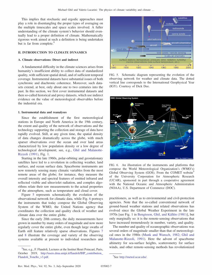
satellites have led to a revolution in collecting weather, landsurface, and ocean surface data. Spaceborne instruments arenow remotely sensing many climatic variables from the mostremote areas of the globe; for instance, they measure theoverall intensity and spectral features of emitted infrared andreflected visible and ultraviolet radiation, and complex algo-rithms relate their raw measurements to the actual propertiesof the atmosphere, such as temperature and cloud cover.Figure 5 represents schematically the evolution of the

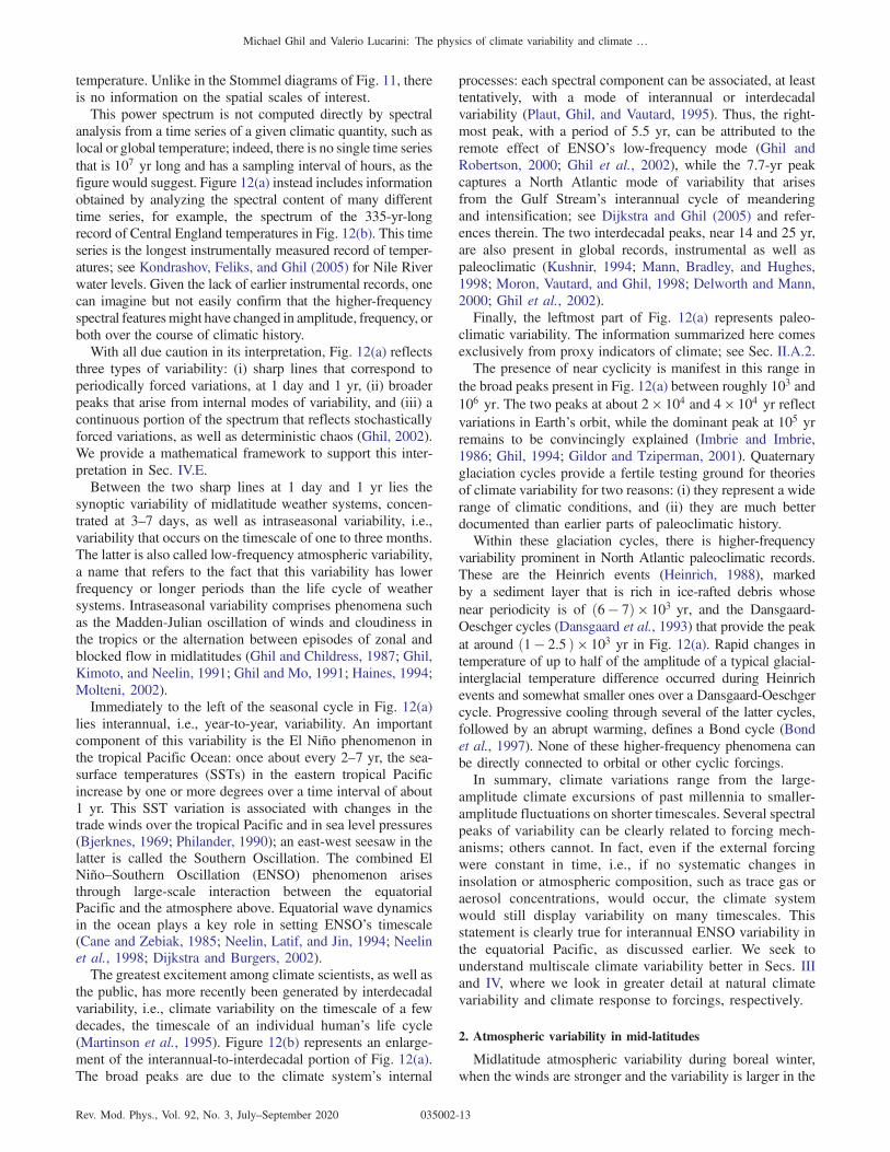
observational network for climatic data, while Fig. 6 portraysthe instruments that today compose the Global ObservingSystem of the WMO, the United Nations agency thatcoordinates the collection and quality check of weather andclimate data over the entire globe.Since the early 20th century, the daily measurements have

grown in number by many orders of magnitude and now moreregularly cover the entire globe, even though large swaths ofEarth still feature relatively sparse observations. Figures 7and 8 illustrate the coverage and variety of the observingsystems available at present to individual researchers and

practitioners, as well as to environmental and civil-protectionagencies. Note that the so-called conventional network ofground-based weather stations and related observations hasevolved since the Global Weather Experiment in the late1970s [see Fig. 1 in Bengtsson, Ghil, and Kallen (1981)], butonly marginally so: it is the remote-sensing observations thathave increased tremendously in number, variety, and quality.The number and quality of oceanographic observations was

several orders of magnitude smaller than that of meteorologi-cal ones in the 1980s (Munk and Wunsch, 1982; Ghil andMalanotte-Rizzoli, 1991). Here the advent of spacebornealtimetry for sea-surface heights, scatterometry for surfacewinds, and other remote-sensing methods has revolutionized

FIG. 5. Schematic diagram representing the evolution of theobserving network for weather and climate data. The dottedvertical line corresponds to the International Geophysical Year(IGY). Courtesy of Dick Dee.

FIG. 6. An illustration of the instruments and platforms thatcompose the World Meteorological Organization’s (WMO’s)Global Observing System (GOS). From the COMET website9

of the University Corporation for Atmospheric Research(UCAR), sponsored in part through a cooperative agreementwith the National Oceanic and Atmospheric Administration(NOAA), U.S. Department of Commerce (DOC).

9See http://meted.ucar.edu/.

8See, e.g., F. Flandoli, Lectures at the Institut Henri Poincare, Paris,October 2019, http://users.dma.unipi.it/flandoli/IHP_contribution_Flandoli_Tonello_v3.pdf.



http://meted.ucar.edu/



http://users.dma.unipi.it/flandoli/IHP_contribution_Flandoli_Tonello_v3.pdf






the field; see, e.g., Robinson (2010). This number, however, isstill smaller by at least 1 order of magnitude than that ofatmospheric observations since, as pointed out by Munk and

Wunsch (1982), the ocean’s interior is not permeable toexploration by electromagnetic waves. This is a fundamentalbarrier hindering our ability to directly observe the deep ocean.Observational data for the atmosphere and ocean are at any

rate sparse, irregular, and of different degrees of accuracy,while in many applications one has to obtain the best estimate,

FIG. 7. Maps of point observations from theWMO’s GOS on 10 April 2009: (a) synoptic weather station and ship reports, (b) upper-airstation reports, (c) buoy observations, (d) aircraft wind and temperature, (e) wind profiler reports, (f) temperature and humidity profilesfrom Global Positioning System (GPS) radio occultation, and (g) observations from citizen weather observers. The tropics are the brightareas bordered by �30° latitude. From the COMETwebsite10 of the UCAR, sponsored in part through cooperative agreements with theNOAA, U.S. DOC.

10See http://meted.ucar.edu/.






with known error bars, of the state of the atmosphere or oceanat a given time and with a given, uniform spatial resolution.More often than not, this estimate also needs to includemeteorological, oceanographic, or coupled-system variables,such as vertical wind velocity and surface heat fluxes, that canbe observed only either poorly or not at all.The active field of data assimilation has been developed

to bridge the gap between the observations that are,typically, discrete in both time and space and the continuumof the atmospheric and oceanic fields. Data assimilation, asdistinct from polynomial interpolation, statistical regression,or the inverse methods used in solid-earth geophysics, firstarose in the late 1960s from the needs of numerical weatherprediction (NWP), on the one hand, and the appearanceof time-continuous data streams from satellites, on the otherhand (Charney, Halem, and Jastrow, 1969; Ghil, Halem,and Atlas, 1979). NWP is essentially an initial-valueproblem for the partial differential equations (PDEs) gov-erning large-scale atmospheric flows (Richardson, 1922)that needed a complete and accurate initial state every 12 or24 hours.

Data assimilation combines partial and inaccurate obser-vational data with a dynamic model, based on physical laws,that governs the evolution of the continuous medium understudy to provide the best estimates of the state of the medium.This model is also subject to errors, due to incompleteknowledge of the smaller-scale processes, numerical discre-tization errors, and other factors. Given these two sources ofinformation, observational and physicomathematical, thereare three types of problems that can be formulated and solvedgiven measurements over a time interval ft0 ≤ t ≤ t1g: filter-ing, smoothing, and prediction; see Fig. 9.Filtering involves obtaining a best-possible estimate of the

state XðtÞ at t ¼ t1, smoothing at all times t0 ≤ t ≤ t1, andprediction at times t > t1. Filtering and prediction are typi-cally used in NWP and can be considered the generation ofshort “video loops,” while smoothing is typically used inclimate studies and resembles the generation of long “featuremovies” (Ghil and Malanotte-Rizzoli, 1991).Figure 10 illustrates a so-called forecast-assimilation cycle,

as used originally in NWP: at evenly spaced, preselectedtimes ftk∶k ¼ 1; 2;…; Kg, one obtains an analysis of the state

FIG. 8. Geographic distribution of observing systems: (a) geostationary satellite observations, (b),(c) polar-orbiting satellite soundings,(d) ocean surface scatterometer-derived winds, and (e),(f) Tropical Rainfall Measuring Mission (TRMM) Microwave Imager orbits.Each color represents the coverage of a single satellite. Observations in (b) and (c) represent vertical layers and area-averaged values.The tropics are marked by the lighter areas bordered by �30° latitude. From the same source as Fig. 7.



XðtkÞ by combining the observations over some intervalpreceding the time tk with the forecast from the previousstate Xðtk−1Þ (Bengtsson, Ghil, and Kallen, 1981; Kalnay,2003). Many variations on this relatively simple scheme havebeen introduced in adapting it to oceanographic data [see Ghiland Malanotte-Rizzoli (1991) and references therein] andspace plasmas [see, e.g., Merkin et al. (2016)] or to usingthe time-continuous stream of remote-sensing data (Ghil,Halem, and Atlas, 1979). Carrassi et al. (2018) provided acomprehensive review of data assimilation methodology andapplications.Analyses are routinely used for numerical weather forecasts

and take advantage of the continuous improvements of modelsand observations. But climate studies require data of con-sistent spatial resolution and accuracy over long time intervals,over which an operational NWP center might have changed itsnumerical model or its data assimilation scheme, as well as itsraw data sources. To satisfy this need, several NWP centershave started in the 1990s to produce so-called reanalyses thatuse the archived data over multidecadal time intervals,typically since World War II, as well as the best model anddata assimilation method available at the time of the reanalysisproject. For obvious reasons of computational cost, reanalysesare often run at a lower spatial resolution than the latestversion in operational use at the time.

Some leading examples of such diachronically coherentreanalyses for the atmosphere are those produced by theEuropean Centre for Medium-Range Weather Forecasts(ECMWF) (Dee et al., 2011), the NCEP-NCAR reanalysisproduced as a collaboration of the U.S. National Centers forEnvironmental Prediction (NCEP) and the National Center forAtmospheric Research (NCAR) (Kistler et al., 2001), and theJRA-25 reanalysis produced by the Japan MeteorologicalAgency (Onogi et al., 2007). While these reanalyses agreefairly well for fields that are relatively well observed, such asthe geopotential field (see Sec. II.C) over the continents of theNorthern Hemisphere, substantial differences persist in theirfields over the Southern Hemisphere or those that are observedeither poorly or not at all (Dell’Aquila et al., 2005, 2007;Kharin, Zwiers, and Zhang, 2005; Marques et al., 2009;Marques, Rocha, and Corte-Real, 2010; Kim and Kim, 2013).Compo et al. (2011) produced a centennial reanalysis from

1871 to the present by assimilating only surface pressurereports and using observed monthly sea-surface temperatureand sea-ice distributions as boundary conditions, while Poliet al. (2016) provided a similar product for the time interval1899–2010, where the surface pressure and the surface windswere assimilated. These enterprises are motivated by the needto provide a benchmark for testing the performance of climatemodels for the late 19th and the 20th century.A similar need has arisen for the ocean: on the one hand,

several much more sizable data sources have become availablethrough remote sensing and have led to detailed oceanmodeling; on the other hand, the study of the coupled climatesystem requires a more uniform dataset, albeit one lessaccurate than for the atmosphere alone. Thus, the equivalentof a reanalysis for the ocean had to be produced, in spite of thefact that the equivalent of NWP for the ocean did not exist. Agood example of a diachronically coherent dataset for theglobal ocean is the Simple Ocean Data Assimilation (Cartonand Giese, 2008). More recently the community of oceanmodelers and observationalists delivered several ocean rean-alyses able to provide a robust estimate of the state of theocean (Lee et al., 2009; Balmaseda et al., 2015).Finally, by relying on recent advances in numerical meth-

ods and in the increased availability of observational data, aswell as of increased performance of computing and storagecapabilities, coupled atmosphere-ocean data assimilation sys-tems have been constructed; see, e.g., Penny and Hamill(2017). Vannitsem and Lucarini (2016) provided a theoreticalrationale for the need of coupled data assimilation schemes tobe able to deal effectively with the climate system’s multiscaleinstabilities. These coupled systems play a key role in effortsto produce seamless weather, subseasonal-to-seasonal (S2S),seasonal, and interannual climate predictions (Palmer et al.,2008; Robertson and Vitart, 2018); they have already beenused for constructing climate reanalyses; see, e.g., Karspecket al. (2018) and Laloyaux et al. (2018).

2. Proxy data

As already mentioned repeatedly and discussed in greaterdetail in Sec. II.B, climate variability covers a vast range oftimescales, and the information we can garner from theinstrumental record is limited to the last century or two.

FIG. 10. Schematic diagram of a forecast-assimilation cyclethat is used for constructing the best estimates of the state ofthe atmosphere, ocean, or both through the procedure of dataassimilation. Observational data are dynamically interpolatedusing the a meteorological, oceanographic, or coupled model toyield the analysis products. The red arrow corresponds to a longerforecast, made only from time to time. Greater detail for the caseof operational weather prediction appears in Ghil (1989), Fig. 1.

FIG. 9. Schematic diagram of filtering F, smoothing S,and prediction P; green solid circles are observations. FromWiener, 1949.



Even so-called historical records extend only to the fewmillennia of a literate humanity (Lamb, 1972). To extendour reach beyond this eyeblink of the planet’s life, it isnecessary to resort to indirect measures of past climaticconditions able to inform us about its state thousands or evenmillions of years ago.Climate proxies are physical, chemical, or biological

characteristics of the past that have been preserved in variousnatural repositories and that can be correlated with the local orglobal state of the atmosphere, ocean, or cryosphere at thattime. Paleoclimatologists and geochemists currently take intoconsideration multiple proxy records, including coral records(Boiseau, Ghil, and Juillet-Leclerc, 1999; Karamperidou et al.,2015) and tree rings (Esper, Cook, and Schweingruber, 2002)for the last few millennia, as well as marine-sediment(Duplessy and Shackleton, 1985; Taricco et al., 2009) andice-core (Jouzel et al., 1993; Andersen et al., 2004) records forthe last 2 × 106 yr of Earth’s history, the Quaternary.Glaciation cycles, i.e., an alternation of warmer and colderclimatic episodes, dominated the latter era. The chemical andphysical characteristics, along with the accumulation rate ofthe samples, require suitable calibration and dating and areused thereafter to infer some of the properties of the climateof the past; see, e.g., Ghil (1994) and Cronin (2010) andreferences therein.Proxies differ enormously in terms of precision, uncertain-

ties in the values and dating, and spatiotemporal extent, andthey do not homogeneously cover Earth. It is common practiceto combine and cross-check many different sources of data tohave a more precise picture of the past (Imbrie and Imbrie,1986; Cronin, 2010). Recently data assimilation methods havestarted to be applied to this problem as well, using simplemodels and addressing the dating uncertainties in particular;see, e.g., Roques et al. (2014). Combining the instrumentaland proxy data with their extremely different characteristics ofresolution and accuracy is a complex and sometimes con-troversial exercise in applied statistics. An important exampleis that of estimating the globally averaged surface air temper-ature record well before the industrial era; see Fig. 4 and theprevious discussion of the hockey stick controversy inSec. I.B.2.

B. Climate variability on multiple Timescales

The presence of multiple scales of motions in space andtime in the climate system can be summarized through so-called Stommel diagrams. Figure 11(a) presents the originalStommel (1963) diagram, in which a somewhat idealizedspectral density associated with the ocean’s variability wasplotted in logarithmic spatial and temporal scales whilecharacteristic oceanic phenomena whose variance exceedsthe background level were identified. Stommel diagramsdescribe the spatial-temporal variability in a climatic sub-domain by associating different, phenomenologically well-defined dynamical features, such as cyclones and long wavesin the atmosphere or meanders and eddies in the ocean, withspecific ranges of scales; they emphasize relationshipsbetween spatial and temporal scales of motion. Usually,specific dynamical features are associated with specific

FIG. 11. Idealized wavelength-and-frequency power spectra forthe climate system. (a) The original Stommel diagram representingthe spectral density (vertical coordinate) of the ocean’s variabilityas a function of the spatial and temporal scale. From Stommel,1963(b) Diagram qualitatively representing the main features ofocean variability. Courtesy of D. Chelton. (c) The same as (b),describing here the variability of the atmosphere.



approximate balances governing the properties of the evolu-tion equations of the geophysical fluids; see Sec. II.C.2.In Figs. 11(b) and 11(c), a qualitative Stommel diagram

portrays today’s estimates of the main range of spatial andtemporal scales in which variability is observed for the oceanand the atmosphere, respectively. One immediately noticesthat larger spatial scales are typically associated with longertemporal scales, in both the atmosphere and the ocean. Thetwo plots show that for both geophysical fluids a “diagonal” ofhigh spectral density in the wavelength-frequency planepredominates. As the diagonal reaches the size of the planetin space, the variability can no longer maintain this propor-tionality of scales and keeps increasing in timescales, whichare not bounded, while the spatial ones are.Both extratropical cyclones in the atmosphere and eddies

in the ocean are due to baroclinic instability, but theircharacteristic spatial extent in the ocean is 10 times smallerand their characteristic duration is 100 times longer thanin the atmosphere. In Fig. 11(c), three important meteoro-logical scales are explicitly mentioned: the microscale(small-scale turbulence), the mesoscale (e.g., thunderstormsand frontal structures), and the synoptic scale (e.g., extra-tropical cyclones).Given the different dynamical variability ranges in space

and time, different classes of numerical models based ondifferent dynamical balances can simulate explicitly onlyone or a few such dynamical ranges. The standard way ofmodeling processes associated with a particular range ofscales is to “freeze” processes on slower timescales or toprescribe their slow quasiadiabatic effect on the variabilitybeing modeled to handle the processes that are too large or tooslow in scale to be included in the model.As for the faster processes, these are “parametrized”; i.e.,

one attempts to model their net effect on the variability ofinterest. Such parametrizations have been, until recently,purely deterministic but have started over the last decade orso to be increasingly stochastic; see Palmer and Williams(2009) and references therein. We discuss the mathematicsbehind parametrizations and provide a few examples inSec. III.G.To summarize, there are about 15 orders of magnitude in

space and in time that are active in the climate system, fromcontinental drift at millions of years to cloud processes athours and shorter increments. The presence of such a widerange of scales in the system provides a formidable challengefor its direct numerical simulation. There is no numericalmodel that can include all the processes that are active on thevarious spatial and temporal scales and can run for 107

simulated years. Occam’s razor and its successors, includingPoincare’s parsimony principle (Poincare, 1902), suggest thatif we had one, it would not necessarily be such a good tool fordeveloping scientific insight. It would instead just be agigantic simulator not helping scientists to distinguish theforest from the trees.Still, there are increasing efforts for achieving “seemless

prediction” across timescales and space scales; see, e.g.,Palmer et al. (2008) and Robertson and Vitart (2018).Merryfield et al. (2020) provided a comprehensive reviewof the most recent efforts for bridging the gap between S2Sand seasonal-to-decadal predictions.

1. A survey of climatic timescales

Combining proxy and instrumental data allows one togather information not only on the mean state of the climatesystem but also on its variability on many different scales. Anartist’s rendering of climate variability in all timescales isprovided in Fig. 12(a). The first version of this figure wasproduced by Mitchell (1976), and many versions thereof havecirculated since. The figure is meant to provide semiquanti-tative information on the spectral power S ¼ SðωÞ, where theangular frequency ω is 2π times the inverse of the oscillationperiod; SðωÞ is supposed to give the amount of variability in agiven frequency band for a generic climatic variable, althoughone typically has in mind the globally averaged surface air

FIG. 12. Power spectra of climate variability across timescales.(a) An artist’s rendering of the composite power spectrum ofclimate variability for a generic climatic variable, from hours tomillions of years; it shows the amount of variance in eachfrequency range. (b) Spectrum of the Central England temper-ature time series from 1650 to the present. Each peak in thespectrum is tentatively attributed to a physical mechanism; seePlaut, Ghil, and Vautard (1995) for details. From Ghil, 2002.



temperature. Unlike in the Stommel diagrams of Fig. 11, thereis no information on the spatial scales of interest.This power spectrum is not computed directly by spectral

analysis from a time series of a given climatic quantity, such aslocal or global temperature; indeed, there is no single time seriesthat is 107 yr long and has a sampling interval of hours, as thefigure would suggest. Figure 12(a) instead includes informationobtained by analyzing the spectral content of many differenttime series, for example, the spectrum of the 335-yr-longrecord of Central England temperatures in Fig. 12(b). This timeseries is the longest instrumentally measured record of temper-atures; see Kondrashov, Feliks, and Ghil (2005) for Nile Riverwater levels. Given the lack of earlier instrumental records, onecan imagine but not easily confirm that the higher-frequencyspectral featuresmight have changed in amplitude, frequency, orboth over the course of climatic history.With all due caution in its interpretation, Fig. 12(a) reflects

three types of variability: (i) sharp lines that correspond toperiodically forced variations, at 1 day and 1 yr, (ii) broaderpeaks that arise from internal modes of variability, and (iii) acontinuous portion of the spectrum that reflects stochasticallyforced variations, as well as deterministic chaos (Ghil, 2002).We provide a mathematical framework to support this inter-pretation in Sec. IV.E.Between the two sharp lines at 1 day and 1 yr lies the

synoptic variability of midlatitude weather systems, concen-trated at 3–7 days, as well as intraseasonal variability, i.e.,variability that occurs on the timescale of one to three months.The latter is also called low-frequency atmospheric variability,a name that refers to the fact that this variability has lowerfrequency or longer periods than the life cycle of weathersystems. Intraseasonal variability comprises phenomena suchas the Madden-Julian oscillation of winds and cloudiness inthe tropics or the alternation between episodes of zonal andblocked flow in midlatitudes (Ghil and Childress, 1987; Ghil,Kimoto, and Neelin, 1991; Ghil and Mo, 1991; Haines, 1994;Molteni, 2002).Immediately to the left of the seasonal cycle in Fig. 12(a)

lies interannual, i.e., year-to-year, variability. An importantcomponent of this variability is the El Niño phenomenon inthe tropical Pacific Ocean: once about every 2–7 yr, the sea-surface temperatures (SSTs) in the eastern tropical Pacificincrease by one or more degrees over a time interval of about1 yr. This SST variation is associated with changes in thetrade winds over the tropical Pacific and in sea level pressures(Bjerknes, 1969; Philander, 1990); an east-west seesaw in thelatter is called the Southern Oscillation. The combined ElNiño–Southern Oscillation (ENSO) phenomenon arisesthrough large-scale interaction between the equatorialPacific and the atmosphere above. Equatorial wave dynamicsin the ocean plays a key role in setting ENSO’s timescale(Cane and Zebiak, 1985; Neelin, Latif, and Jin, 1994; Neelinet al., 1998; Dijkstra and Burgers, 2002).The greatest excitement among climate scientists, as well as

the public, has more recently been generated by interdecadalvariability, i.e., climate variability on the timescale of a fewdecades, the timescale of an individual human’s life cycle(Martinson et al., 1995). Figure 12(b) represents an enlarge-ment of the interannual-to-interdecadal portion of Fig. 12(a).The broad peaks are due to the climate system’s internal

processes: each spectral component can be associated, at leasttentatively, with a mode of interannual or interdecadalvariability (Plaut, Ghil, and Vautard, 1995). Thus, the right-most peak, with a period of 5.5 yr, can be attributed to theremote effect of ENSO’s low-frequency mode (Ghil andRobertson, 2000; Ghil et al., 2002), while the 7.7-yr peakcaptures a North Atlantic mode of variability that arisesfrom the Gulf Stream’s interannual cycle of meanderingand intensification; see Dijkstra and Ghil (2005) and refer-ences therein. The two interdecadal peaks, near 14 and 25 yr,are also present in global records, instrumental as well aspaleoclimatic (Kushnir, 1994; Mann, Bradley, and Hughes,1998; Moron, Vautard, and Ghil, 1998; Delworth and Mann,2000; Ghil et al., 2002).Finally, the leftmost part of Fig. 12(a) represents paleo-

climatic variability. The information summarized here comesexclusively from proxy indicators of climate; see Sec. II.A.2.The presence of near cyclicity is manifest in this range in

the broad peaks present in Fig. 12(a) between roughly 103 and106 yr. The two peaks at about 2 × 104 and 4 × 104 yr reflectvariations in Earth’s orbit, while the dominant peak at 105 yrremains to be convincingly explained (Imbrie and Imbrie,1986; Ghil, 1994; Gildor and Tziperman, 2001). Quaternaryglaciation cycles provide a fertile testing ground for theoriesof climate variability for two reasons: (i) they represent a widerange of climatic conditions, and (ii) they are much betterdocumented than earlier parts of paleoclimatic history.Within these glaciation cycles, there is higher-frequency

variability prominent in North Atlantic paleoclimatic records.These are the Heinrich events (Heinrich, 1988), markedby a sediment layer that is rich in ice-rafted debris whosenear periodicity is of ð6 − 7Þ × 103 yr, and the Dansgaard-Oeschger cycles (Dansgaard et al., 1993) that provide the peakat around ð1 − 2.5 Þ × 103 yr in Fig. 12(a). Rapid changes intemperature of up to half of the amplitude of a typical glacial-interglacial temperature difference occurred during Heinrichevents and somewhat smaller ones over a Dansgaard-Oeschgercycle. Progressive cooling through several of the latter cycles,followed by an abrupt warming, defines a Bond cycle (Bondet al., 1997). None of these higher-frequency phenomena canbe directly connected to orbital or other cyclic forcings.In summary, climate variations range from the large-

amplitude climate excursions of past millennia to smaller-amplitude fluctuations on shorter timescales. Several spectralpeaks of variability can be clearly related to forcing mech-anisms; others cannot. In fact, even if the external forcingwere constant in time, i.e., if no systematic changes ininsolation or atmospheric composition, such as trace gas oraerosol concentrations, would occur, the climate systemwould still display variability on many timescales. Thisstatement is clearly true for interannual ENSO variability inthe equatorial Pacific, as discussed earlier. We seek tounderstand multiscale climate variability better in Secs. IIIand IV, where we look in greater detail at natural climatevariability and climate response to forcings, respectively.

2. Atmospheric variability in mid-latitudes

Midlatitude atmospheric variability during boreal winter,when the winds are stronger and the variability is larger in the



Northern Hemisphere, has long been a major focus ofdynamic meteorology. The intent of this section is to motivatethe reader to appreciate the complexity of large-scale atmos-pheric dynamics by focusing on a relatively well understoodaspect thereof. We see that fairly diverse processes contributeto the spectral features discussed in connection with Fig. 12.The synoptic disturbances that are most closely associated

with midlatitude weather have characteristic timescales ofthe order of 3–10 days, with a corresponding spatial scale ofthe order of 1000–2000 km (Holton and Hakim, 2013). Theyroughly correspond to the familiar eastward-propagatingcyclones and anticyclones and emerge as a result of theprocess of baroclinic instability, which converts availablepotential energy of the zonal flow into eddy kinetic energy.This conversion is a crucial part of the Lorenz energy cycle

(Lorenz, 1955, 1967), and it occurs through the lowering ofthe center of mass of the atmospheric system undergoing anunstable development. Baroclinic instability (Charney, 1947;Vallis, 2006; Holton and Hakim, 2013) is active when themeridional temperature gradient or, equivalently, the verticalwind shear is strong enough. These conditions are morereadily verified in the winter season, which features a largeequator-to-pole temperature difference and a strong midlati-tude jet (Speranza, 1983; Holton and Hakim, 2013).The space-time spectral analysis introduced by Hayashi

(1971) and refined by Pratt (1976) and Fraedrich and Bottger(1978) builds upon the idea of the Stommel diagrams in Fig. 11.In addition, it provides information about the direction andspeed at which the atmospheric eddies move and associateswith each range of spatial and temporal scales a correspondingweight in terms of spectral power. This information may beobtained in the first instance by Fourier analysis of a one-dimensional spatial field, and it allows one to reconstruct thepropagation of atmospheric waves. This analysis is usuallycarried out in the so-called zonal, i.e., west-to-east, direction;see Sec. II.C.Next one can compute the power spectrum in the frequency

domain for each spatial Fourier component and then averagethe results across consecutive winters to derive a climatologyof winter atmospheric waves. The difficulty here lies in thefact that straightforward space-time decomposition does notdistinguish between standing and traveling waves: a standingwave gives two spectral peaks corresponding to waves thattravel eastward and westward at the same speed and with thesame phase. This problem can be circumvented only bymaking assumptions regarding a given wave’s nature. Forinstance, we may assume complete coherence between theeastward and westward components of standing waves andattribute the incoherent part of the spectrum to actualtraveling waves.Figure 13 shows the spectral properties of the winter

500-hPa geopotential height field meridionally averagedacross the midlatitudes of the northern hemisphere (specifi-cally, between 30° and 75° N) for the time interval 1957–2002.The properties of all waves, as well as the standing, eastward-traveling, and westward-traveling waves, appear in panelsFigs. 13(a)–13(d), respectively. As discussed later, the 500-hPaheight field provides a synthetic yet comprehensive picture ofthe atmosphere’s synoptic to large-scale dynamics.

Figure 13(c) shows that the eastward-propagating wavesare dominated by synoptic variability, concentrated over3–12-day periods and zonal wave numbers 5–8; note that asingle cyclone or anticyclone counts for half a wavelength.In addition, the slanting high-variability ridge in HE indicatesthe existence of a statistically defined dispersion relation thatrelates frequency and wave number, which is in agreementwith the basic tenets of baroclinic instability theory (Holtonand Hakim, 2013).When looking at the westward-propagating variance in

Fig. 13(d), one finds that the dominant portion of thevariability is associated with low-frequency, planetary-scaleRossby waves. Finally, Fig. 13(b) shows the contribution tothe variance given by standing waves, which correspond tolarge-scale, geographically locked, and persistent phenomenalike blocking events. Note that westward-propagating andstationary waves provide the lion’s share of the overallvariability of the atmospheric field; see also Kimoto andGhil (1993a), Fig. 7.The dynamics and energetics of planetary waves are still

under intensive scrutiny. Descriptions and explanations ofseveral highly nonlinear aspects thereof are closely inter-woven with those of blocking events, identified as persistent,large-scale deviations from the zonally symmetric generalcirculation (Charney and DeVore, 1979; Legras and Ghil,1985; Benzi et al., 1986; Ghil and Childress, 1987; Benzi andSperanza, 1989; Kimoto and Ghil, 1993a). Weeks et al.(1997) provided a fine example of contrast between a blockingevent and the climatologically more prevalent zonal flow.Persistent blocking events strongly affect the weather for

up to a month over continental-size areas. Such persistenceoffers some hope for extended predictability of large-scaleflows, and of the associated synoptic-scale weather, beyondthe usual predictability of the latter, which is believed notto exceed 10–15 days; see Lorenz (1996) and referencestherein.Today, the most highly resolved and physically detailed

NWPmodels are reasonably good at predicting the persistenceof a blocking event once the model’s initial state is within thatevent, but not at predicting the onset of such an event or itscollapse (Ferranti, Corti, and Janousek, 2015). Likewise, thecapability of necessarily lower-resolution climate models tosimulate the spatiotemporal statistics of such events is far fromperfect; in fact, relatively limited improvement has beenrealized in the last two decades (Davini and D’Andrea,2016). Weeks et al. (1997) reproduced successfully in thelaboratory key features of the dynamics and statistics ofblocking events.Ghil and Robertson (2002) reviewed several schematic

descriptions of the midlatitude atmosphere’s low-frequencyvariability (LFV) as jumping between a zonal regime and ablocked one or, more generally, a small number of suchregimes. This coarse graining of the LFV’s phase space andMarkov chain representation of the dynamics continues toinform current efforts at understanding what atmosphericphenomena can be predicted beyond 10–15 days and how.Recently analyses based on dynamical-systems theory haveassociated blocked flow configurations with higher instabilityof the atmosphere as a whole (Schubert and Lucarini, 2016;



Faranda, Messori, and Yiou, 2017; Lucarini and Gritsun,2020), as predicted by Legras and Ghil (1985).The effect of global warming on the statistics of blocking

events has recently become a matter of considerable con-troversy. The sharper increase of near-surface temperatures inthe Arctic than near the Equator is fairly well understood [see,e.g., Ghil (1976), Fig. 7] and has been abundantly documentedin recent observations; see, e.g., Walsh (2014), Fig. 8. Thisdecrease in pole-to-equator temperature difference ΔT isreferred to as polar amplification of global warming.Francis and Vavrus (2012) and Liu et al. (2012) suggested

that reduced ΔT slows down the prevailing westerlies andincreases the north-south meandering of the subtropical jetstream, resulting in more frequent blocking events. Thissuggestion seems to agree with fairly straightforward argu-ments of several other authors on the nature of blocking(Charney and DeVore, 1979; Legras and Ghil, 1985; Ghil andChildress, 1987), as illustrated, for instance, by Ghil andRobertson (2002) in their Fig. 2): The strength ψ�

A of the

driving jet in the figure is proportional to ΔT, in accordancewith standard quasigeostrophic flow theory,11 and lowerjet speeds ψA favor blocking. Ruti et al. (2006) alsopresented observational evidence for a nonlinear relationbetween the strength of the subtropical jet and the probabilityof occurrence of blocking events, in agreement with thebent-resonance theory of midlatitude LFV proposed byBenzi et al. (1986).Considerable evidence against the apparently straightfor-

ward argument for global warming as the cause of an increasein midlatitude blocking has accumulated too from bothobservational and modeling studies; see Hassanzadeh,Kuang, and Farrell (2014), Barnes and Screen (2015), andreferences therein. The issue is far from settled, as are manyquestions about other regional effects of global warming.

FIG. 13. Variance H of the winter (December–February) atmospheric fields in the midlatitudes of the Northern Hemisphere. (a) Totalvariance HT . (b) Variance associated with standing waves HS. (c) Variance associated with eastward-propagating waves HE.(d) Variance associated with westward-propagating waves HW . Based on NCEP-NCAR reanalysis data (Kistler et al., 2001). See thetext for details. From Dell’Aquila et al., 2005.

11See Secs. II.C.2 and II.C.3 for geostrophic balance, quasigeos-trophy, and their consequences.



C. Basic properties and fundamental equations

1. Governing equations

The evolution of the atmosphere, the ocean, the soil, and theice masses can be described by using the continuum approxi-mation, in which these subsystems are represented by fieldvariables that depend on three spatial dimensions and time.For each of the climatic subdomains, we consider thefollowing field variables: the density ρ and the heat capacityat constant volume C, with the specific expression for ρ and Cdefining the thermodynamics of the medium; the concen-tration of the chemical species fξk∶1 ≤ k ≤ Kg contained inthe medium and present in different phases, e.g., the saltdissolved in the ocean or the water vapor in the atmosphere;the three components fvi∶1 ≤ i ≤ 3g of the velocity vector;the temperature T; the pressure p; the heating rate J; and thegravitational potential Φ.Note that by making the thin-shell approximation

H=R ≪ 1, where H is the vertical extent of the geophysicalfluid and R is the radius of Earth, we can assume that thegravitational potential at the local sea level is zero and can thussafely use the approximation Φ ¼ gz, where Φ is then calledthe geopotential, g is the gravity at the surface of Earth, and zis the geometric height above sea level. Moreover, one has totake into account the fact that the climate system is embeddedin a noninertial frame of reference that rotates with an angularvelocity Ω with components fΩi∶1 ≤ i ≤ 3g.The PDEs that govern the evolution of the field variables

are based on the budget of mass, momentum, and energy.When the fluid contains several chemical species, theirseparate budgets also have to be accounted for (Vallis,2006). To have a complete picture of the Earth system,one should in principle also consider the evolution ofbiological species. Doing so, however, is well beyond ourscope here, even though present Earth system models doattempt to represent biological processes, albeit in a sim-plified way; see the discussion in Sec. II.D.The mass budget equations for the constituent species can

be written as follows:

∂tðρξkÞ ¼ −∂iðρξkviÞ þDξk þ Lξk þ Sξk : ð1Þ

Here ∂t is the partial derivative in time and ∂i is the partialderivative in the xi direction;Dξk , Lξk , and Sξk are the diffusionoperator, phase changes, and local mass budget due to otherchemical reactions that are associated with k.The momentum budget’s ith component is written as

∂tðρviÞ ¼ −∂jðρvjviÞ − ∂ipþ ρ∂iΦ

− 2ρϵijkΩjvk þ Ti þ Fi: ð2Þ

Here the Levi-Civita antisymmetric tensor ϵijk is used to writethe Coriolis force; Ti indicates direct mechanical forcings,e.g., those resulting from lunisolar tidal effects; Fi ¼ −∂jτijcorresponds to friction, with fτijg the stress tensor; andsummation over equal indices is used. Equation (2) is justa forced version of the momentum equation in the Navier-Stokes equations (NSEs), written in a rotating frame ofreference.

A general state equation valid for both fluid envelopes ofEarth, i.e., the atmosphere and the ocean, is

ρ ¼ gðT; p; ξ1;…; ξKÞ: ð3Þ

As a first approximation, one can take K ¼ 1, where ξ1 ¼ ξ is,respectively, moisture in the atmosphere and salinity of theocean. For brevity, we restrict ourselves here to the atmosphere.In general, one can write the specific energy of the climate

system as the sum of the specific internal, potential, andkinetic energies, also taking into account the contributionscoming from chemical species in different phases. To getmanageable formulas, some approximations are necessary;see, e.g., Peixoto and Oort (1992).Neglecting reactions other than the phase changes between

the liquid and gas phases of water, the expression of thespecific energy in the atmosphere is

e ¼ cvT þΦþ vjvj=2þ Lq;

where cv is the specific heat at constant volume for thegaseous atmospheric mixture, L is the latent heat of evapo-ration, and q ¼ ρξ is the specific humidity. In this formula, weneglect the heat content of the liquid and solid water and theheat associated with the phase transition between solid andliquid water. Instead, the approximate expression for thespecific energy in the ocean is

e ¼ cWT þΦþ vjvj=2;

where cW is the specific heat at constant volume ofwater, while neglecting the effects of salinity and of pressure.Finally, for the specific energy of soil or ice, we can takee ¼ cfS;IgT þΦ, respectively.After some nontrivial calculations, one derives the follow-

ing general equation for the local energy budget:

∂tðρeÞ ¼ −∂jðρεvjÞ − ∂jQSWj − ∂jQLW

j

− ∂jJSHj − ∂jJLHj − ∂jðviτijÞ þ viTi; ð4Þ

where e is the energy per unit mass and ε ¼ eþ p=ρ is theenthalpy per unit mass. The energy source and sink terms canbe written as the sum of the work done by the mechanicalforcing viTi and of the respective divergences of the short-wave (solar) and longwave (terrestrial) components of thePoynting vector QSW

j and QLWj , of the turbulent sensible and

latent heat fluxes JSHj and JLHj , and of the scalar product of thevelocity field with the stress tensor viτij.Equation (4) is written in a conservative form, with the

right-hand side containing only the sum of flux divergences,except for the last term, which is negligible. By taking suitablevolume integrals of Eq. (4) and assuming steady-state con-ditions, one derives meridional enthalpy transports from thezonal budgets of energy fluxes (Ghil and Childress, 1987;Peixoto and Oort, 1992; Lucarini and Ragone, 2011; Lucarini,Blender et al., 2014); recall Figs. 2(a) and 2(b). The presenceof inhomogeneous absorption of shortwave radiation due tothe geometry of the Sun-Earth system and of the physico-chemical properties of the climatic subdomains determines the



presence of nonequilibrium conditions for the climate system,as already discussed in Sec. I.A.Various versions of Eqs. (1)–(4) have been studied for over

a century, and well-established thermodynamical and chemi-cal laws accurately describe the phase transitions and reactionsof the climate system’s constituents. Finally, quantummechanics allows one to calculate in detail the interactionbetween matter and radiation.Still, despite the fact that climate dynamics is governed

by well-known evolution equations, it is way beyond ourscientific ability to gain a complete picture of the mathemati-cal properties of the solutions. In fact, many fundamentalquestions are still open regarding the basic NSEs in ahomogeneous fluid without phase transitions and rotation(Temam, 1984, 1997). In particular, even for the basic NSEs,providing analytical, closed-form solutions is possible only insome highly simplified cases that are either linear or otherwiseseparable (Batchelor, 1974).As discussed, Eqs. (1)–(4) can simulate a range of phe-

nomena that spans many orders of magnitude in spatial andtemporal scales. Hence, it is virtually impossible to constructnumerical codes able to explicitly represent all ongoingprocesses at the needed resolution in space and time. It isthus necessary to parametrize the processes that occur atsubgrid scales and cannot, therewith, be directly represented.Among the most important processes of this type are cloud-radiation interactions and turbulent diffusion. We discuss thetheoretical framework behind the formulation of parametriza-tions in Sec. III.G.

2. Approximate balances and filtering

Equations (1)–(4) are too general and contain too manywave propagation speeds and instabilities to properly focus oncertain classes of phenomena of interest. For instance, thefluid’s compressibility plays a role only in the propagation ofextremely fast acoustic waves, whose energy is negligible,compared to that of the winds and currents we are interestedin here.Therefore, starting with Charney (1947), more-or-less-

systematic approximations have been introduced to filterout undesirable waves from the equations of motion and tostudy particular classes of phenomena and processes.Depending on the climate subsystem and the range of scalesof interest, different approximations can be adopted. Forexample, if one considers ice sheets and bedrock on thetimescale of millennia, it is reasonable to assume that vj ≃ 0,i.e., to remove the flow field from the evolution equation;see Ghil (1994), Saltzman (2001), and references therein.This approximation is not valid if one wants to describeexplicitly the motion of the ice sheets on shorter timescales(Paterson, 1981).More precisely, the filtering process consists of applying a

set of mathematical approximations to the fundamentalgoverning equations, usually considered to be a suitablegeneralization of the classical NSEs like Eqs. (1)–(4). Thepurpose of this filtering is to exclude from the filtered systemcertain physical processes that are heuristically assumedto play only a minor role in its dynamics at the timescaleand space scale under investigation. The magnitudes of all

terms in the governing equations for a particular type ofmotion are estimated by dimensional analysis (Barenblatt,1987), and various classes of simplified equations have beenderived by considering distinct asymptotic regimes in theassociated scales (Ghil and Childress, 1987; Pedlosky, 1987;McWilliams, 2006; Klein, 2010).The approximations adopted rely on assuming that the

continuous medium, whether fluid or solid, obeys suitablydefined time-independent relations or undergoes only smalldepartures from such relations, and that these relations resultfrom the balance of two or more dominating forces.Imposing such balances leads to reducing the number ofindependent field variables of the system that obey a set ofevolution equations. Additionally, the imposition of dynami-cal balances leads to removing specific wave motions fromthe range of allowed dynamical processes.In meteorological terminology, a prognostic variable whose

tendency, i.e., time derivative, appears in the full equationsmay thus become a diagnostic variable, which appears in anondifferentiated form only in the filtered equations. Next wesee two of the most important examples of filtering, which,among other things, are essential for the practical implemen-tation of numerical models of the atmosphere and ocean(Vallis, 2006; Cushman-Roisin and Beckers, 2011; Holtonand Hakim, 2013).

a. Hydrostatic balance

A classical example of filtering is the hydrostatic approxi-mation. In a local Cartesian coordinate system ðx; y; zÞ, wedefine by z ¼ ∇Φ=j∇Φj the direction perpendicular to ageopotential isosurface Φ≡ const. An obvious stationarysolution of the NSEs is given in these coordinates by thetime-independent hydrostatic balance equation

ρhg ¼ −∂zph; ð5Þ

where the subscript h denotes this solution.On sufficiently large spatial and temporal scales, many

geophysical flows, e.g., atmospheric and oceanic, as well ascontinental surface and ground water, are near hydrostaticequilibrium. In general, stable hydrostatic equilibrium isachieved when fluid with lower specific entropy lies belowfluid with higher specific entropy; in this case, Eq. (5) isobeyed for all ðx; y; zÞ within the domain occupied bythe fluid.When this condition is broken because of external forcing

or internal heating, say, the stratification is not stable and thefluid readjusts so as to reestablish the hydrostatic equilibrium.This readjustment is achieved by vertical convective motions,in which available potential energy is transformed into kineticenergy responsible for vertical motions that can locally bemuch faster than the large-scale flow. Violations of hydrostaticbalance thus exist only on short timescales and space scales.A large class of models used in studying, simulating, and

attempting to predict climate variability and climate changeis based on a particular simplification of the full set ofEqs. (1)–(4). This simplification leads to the so-calledprimitive equations, which filter out nonhydrostatic motions.As a result, sound waves are excluded from the solutions, a



fact that facilitates the numerical implementation of suchmodels (Washington and Parkinson, 2005; Cushman-Roisinand Beckers, 2011).The primitive equations are derived by assuming that

the time-independent hydrostatic balance given in Eq. (5)does apply at all times, even when the flow is time dependent.One thus assumes that the vertical acceleration of the fluid iseverywhere much smaller than gravity. Neglecting the verticalacceleration altogether leads to a monotonic relationshipbetween the vertical coordinate z and pressure p.12

One can hence replace z with p as a vertical coordinate andrewrite the modified Eqs. (1)–(4) using a new coordinatesystem in which one also replaces, typically, the horizontalcoordinates ðx; yÞ by the longitude λ and the latitude ϕ,respectively. In such a coordinate system, v3 ≡ ω≡ ∂tp is thechange of pressure with time, the 3D velocity field is non-divergent ∂jvj ¼ 0, and the density is automatically constantand set to 1 (Vallis, 2006; Holton and Hakim, 2013).Despite the use of primitive equations, climate models aim

at simulating a system that nonetheless features nonhydro-static motions. Additionally, geophysical flows obeyingprimitive equations can lead to unstable vertical configura-tions of the fluids. Typical climate models are formulated toquickly eliminate local nonhydrostatic conditions and toparametrize the balanced condition that is thus recovered interms of variables that are explicitly represented in the model,following the idea of convective adjustment originally pro-posed by Manabe and Strickler (1964). Finding optimalways to parametrize the effect of convection on hydrostaticclimate models has become a key research area in climatedynamics; see Emanuel (1994) for a classical treatise on theproblem of atmospheric convection and Plant and Yano(2016) for a recent overview.The primitive equations were at the core of both climate

models and weather prediction models for three decades, fromabout the 1970s through the 1990s. Nonhydrostatic models,constructed through discretization of the full NSEs withforcing and rotation, have become increasingly available overthe last decade, first as limited-area models and more recentlyeven as global ones; see, e.g., Marshall et al. (1997).These models require extremely high resolution in space

and time and are computationally quite expensive; as they startto enter operational use, they require state-of-the-art hardwareand software, in terms of both computing and storage, as wellas sophisticated postprocessing of the output. Moreover, forall practical purposes sufficiently detailed initial and boundarydata are not available, and methodological problems reappearin connection with formulating such data. Still, the use ofnonhydrostatic models allows, in principle, for bypassing thekey problem of parametrizing convection.

b. Geostrophic balance

Another important example of filtering is the one associatedwith time-independent purely horizontal balanced flows, in

which the horizontal components of the pressure gradientforce and the Coriolis force cancel out in the NSEs. Suchflows are termed geostrophic; etymologically, this meansEarth turning. The nondimensional parameter that determinesthe validity of this approximation is the Rossby numberRo ¼ U=f0L, where U is a characteristic horizontal velocity,L is a characteristic horizontal extent, and f0 ¼ 2Ω sinϕ0;here Ω is the modulus of Earth’s angular frequency of rotationaround its axis and ϕ0 is a reference latitude.The geostrophic approximation provides a good diagnostic

description of the flow when Ro ≪ 1. Such small Ro valuesprevail for the atmosphere on synoptic and planetary scales,such as those of extratropical weather systems, say polewardof 30°, where f0 is large enough, and in the free atmosphere,i.e., above the planetary boundary layer, where frictionalforces can be comparable to the Coriolis force. In the ocean,this approximation is extremely accurate everywhere exceptclose to the equator. The smallness of the Rossby number inthe ocean arises from oceanic currents being orders ofmagnitude slower than atmospheric winds, so Ro nears unityonly where f0 is extremely small.Purely geostrophic flow fields are obtained via a zeroth-

order expansion in Ro of the NSEs. Fluid motion is introducedby considering small perturbations ρg and pg that break thetranslation symmetry of the basic, purely hydrostatic densityand pressure fields ρh and ph but preserve the geostrophicbalance, i.e., one sets ρ ¼ ρh þ ρg and p ¼ ph þ pg,respectively.Letting x be locally the zonal direction and y be locally the

meridional direction, one can write (Holton and Hakim, 2013)the geostrophic balance at each height z as

ρhuf0 ¼ −∂ypg; ð6aÞ

ρhvf0 ¼ ∂xpg; ð6bÞ

where the derivatives are taken at constant z, ðu; vÞ ¼ ðv1; v2Þand, furthermore, the geostrophic perturbation itself is inhydrostatic equilibrium, i.e., gρg ¼ −∂zpg. The combinedhydrostatic and geostrophic balance constrains atmosphericand oceanic motions so that the velocity field is uniquelydetermined by the pressure field. In such doubly balancedflows, the winds or currents are parallel to the isobars at agiven geopotential height z, as shown in Fig. 14(a) ratherthan perpendicular to the isobars, as in nonrotating fluids.Moreover, the vertical component of the velocity fieldvanishes w ¼ v3 ≡ 0.Using the pressure coordinate system ðx; y; pÞ described

previously, where p plays the role of the vertical coordinate,it is possible to express the geostrophic balance as follows(Holton and Hakim, 2013):

f0ug ¼ −∂yΦ; ð7aÞ

f0vg ¼ ∂xΦ; ð7bÞ

where this time derivatives are taken at constant p. Thevertical derivative ∂pΦ can, furthermore, be expressed interms of ρg. For the atmosphere, one can make the simplifying

12The validity of this approximation, even locally in space and atmost times, explains Pascal’s experimental observation during thefamed 1648 Puy-de-Dôme ascension that a barometer’s readingdecreases monotonically with altitude.



assumption of dry conditions, for which the equation of stateis described by the gas constant R and the heat capacity atconstant pressure Cp.Assuming, moreover, a horizontally homogeneous back-

ground state with Th ¼ ThðpÞ, introducing the potentialtemperature Θh ¼ Thðp=psÞR=Cp , with ps ¼ const the refer-ence surface pressure, and letting σ ≔ −RThd lnΘh=dp, whichdefines the stratification of the background state, one obtains

∂pΦ ¼ −Rpσ

Tg: ð8Þ

Thus, in the geostrophic approximation the scalar field Φprovides complete diagnostic information on the state of thefluid: its horizontal derivatives give us the velocity field, whilethe vertical derivative gives us the geopotential, or mass field,via perturbations with respect to the background temperaturefield (Holton and Hakim, 2013).Essentially, geophysical fluid dynamics (GFD) is the study

of large-scale flows dominated by the combined hydrostaticand geostrophic balances. The former is a consequence of theshallowness of the planetary flows, the latter is a consequenceof their rotation (Ghil and Childress, 1987; Pedlosky, 1987;McWilliams, 2006; Cushman-Roisin and Beckers, 2011).Section II.C.3 introduces the more complex situation offinite-but-small perturbations from this combined balance.Although modern computers allow a fully ageostrophic

(beyond geostrophic approximation) description of most geo-physical fluids, geostrophic balance remains a fundamental toolof theoretical research, and it is also used for practical applica-tions in everyday weather prediction. Figure 14(b) illustratesa typical midlatitude synoptic situation: at a given pressurelevel, the winds blow, to a good approximation, parallel to theisolines of geopotential height, and the speed of the wind ishigher where the gradient of geopotential height is stronger. Anappendix in Ghil, Halem, and Atlas (1979) describes the extentto which diagnostic relations based on the geostrophic approxi-mation are still used in the analysis and prediction of midlatitudeweather, as simulated by advanced numerical models. Indeed,geostrophic approximation is implicit in the day-to-day readingof weather maps on synoptic-to-planetary scales.

3. Quasigeostrophy and weather forecasting

The diagnostic, i.e., time-independent nature of the geo-strophic balance, implies that the ageostrophic terms, althoughrelatively small, are important for the time evolution of theflow. A planetary flow that evolves slowly in time comparedto 1=f0 can be described using quasigeostrophic theory,namely, a perturbative theory that expands the NSEs in Roand truncates at first order.The use of the quasigeostrophic approximation effectively

filters out solutions that correspond to higher-speed atmos-pheric or oceanic inertia-gravity waves; the latter, also calledPoincare waves, are gravity waves modified by the presenceof rotation (Ghil and Childress, 1987; Pedlosky, 1987;McWilliams, 2006; Vallis, 2006; Cushman-Roisin andBeckers, 2011; Holton and Hakim, 2013). This approximationbreaks down, though, near frontal discontinuities and in othersituations in which the ageostrophic component of the velocityfield plays an important advective role, and it has to beimproved upon by retaining higher-order terms.In quasigeostrophic theory, a fundamental role is played by

the quasigeostrophic potential vorticity14

q ¼ 1

f0Δ2Φþ f þ ∂p

�f0σ∂pΦ

�: ð9Þ

FIG. 14. Geostrophic balance. (a) Schematics of geostrophicallybalanced flow in the Northern Hemisphere. At a given z level, thepressure gradient force (upward-pointing arrow) and Coriolis force(downward-pointing arrow) cancel out and the flow (horizontalarrow) is parallel to the isobars. (b) Synoptic conditions for the500-hPa level over the United States at 0000 Greenwich MeanTime (GMT) on 12 July 2019. The dark gray lines indicate theisolines of geopotential height z ¼ Φ=g (in units of 10 m), and thebarbed blue arrows indicate the direction of the wind; the barbsindicate the wind speed, with each short (long) barb correspondingto a speed of 5 knots (10 knots), with 2 knots ¼ 1.03 ms−1. Fromthe NOAA-National Weather Service.13

13See https://www.spc.noaa.gov/obswx/maps/.

14More general formulations of potential vorticity are also quiteimportant in GFD; see, e.g., Hoskins, McIntyre, and Robertson(1985).



https://www.spc.noaa.gov/obswx/maps/




Here Δ2 is the horizontal Laplacian in p coordinates, the firstterm ζg ¼ Δ2Ψ=f0 is the relative vorticity of the geostrophicflow, f is the planetary vorticity, and the last term is thestretching vorticity; the static stability σ, which measures thestratification of the fluid, was introduced in Eq. (8).The potential vorticity q thus combines dynamical and

thermodynamical information on the fluid flow. In moreabstract terms, one can write

q − f ¼ LΦ; ð10Þ

where L is a modified three-dimensional Laplacian operator.Using suitable boundary conditions, one can invert Eq. (10)and derive the geopotential field from the vorticity field

Φ ¼ L−1ðq − fÞ: ð11Þ

In the absence of forcing and dissipation, q is conserved bygeostrophic motions so that

∂tqþ J

�Φf0

; q

�¼ 0; ð12Þ

where JðA; BÞ ¼ ∂xA∂yB − ∂yA∂xB is the Jacobian operator,so JðΦ=f0; qÞ ¼ ð1=f0Þð∂xΦ=∂yq − ∂yΦ∂xqÞ describes vor-ticity advection by the geostrophic velocity field ðug; vgÞ; seeEq. (6). Note that in the limit σ → ∞, i.e., if one assumesinfinitely stable stratification, the third term on the right-hand side of Eq. (9) drops out and Eq. (12) describes theconservation of the absolute vorticity in a barotropic two-dimensional flow.Quasigeostrophic theory, as introduced by Charney (1947),

arguably provided a crucial advance for the understanding ofthe dynamics of planetary flows and provided the foundationfor the successful start of NWP (Charney, Fjørtoft, and vonNeumann, 1950). The filtering associated with this theorywas, in particular, instrumental in eliminating the numericalinstability that marred the pioneering weather forecast experi-ment of Richardson (1922).In fact, L. F. Richardson used a more accurate set of

equations of motion for the atmosphere than the set ofEqs. (9)–(12). Somewhat counterintuitively, the quasigeo-strophic model eventually provided a more accurate predictiontool because it represented more robustly the dynamicalprocesses at the scales of interest. The inconclusive result ofRichardson’s one-step, 6-h numerical experiment was receivedby the meteorological community at the time as proof thatNWP, as proposed by Bjerknes (1904), was not possible.We outline herewith how the quasigeostrophic potential-

vorticity equations can be used to perform stable numericalweather forecasts. Assume that at time t ¼ t0 we haveinformation on the geopotential height field Φ0 ¼ Φðt0Þ.

• Step 0: Using Eq. (10), one computes the corre-sponding potential vorticity field q0 ¼ qðt0Þ.

• Step A: Equation (12) is used next to predict thepotential vorticity field at time t1 as follows: q1¼qðt1Þ¼qðt0ÞþJðΦ0=f0;q0ÞΔt, where Δt ¼ t1 − t0.

• Step B: Equation (11) is used now to infer Φ1.• Step C: Go to step A and predict q2, etc.

Three decades after Richardson (1922), Charney, Fjørtoft,and von Neumann (1950) performed the first successfulnumerical weather forecasts on the ENIAC computer inPrinceton by using essentially the same procedure detailedpreviously for the simpler case of barotropic two-dimensionalflow. In this case, the standard absolute vorticity is given bythe sum of relative and planetary vorticity, and it plays a roleanalogous to potential vorticity in quasigeostrophic three-dimensional flow. The procedure was adapted to describethe evolution of the 500-hPa field, which deviates the leastfrom the behavior of an idealized atmosphere of homogeneousdensity with no vertical velocities. The simulation wasperformed on a limited domain that covered North Americaand the adjacent ocean areas.Charney, Fjørtoft, and von Neumann investigated the issues

associated with horizontal boundary conditions, as well aswith the numerical stability of the integration. Their success(Charney, Fjørtoft, and von Neumann, 1950) paved the wayfor the theory’s successive applications to physical oceanog-raphy and climate dynamics as a whole (Ghil and Childress,1987; Pedlosky, 1987; Dijkstra, 2005). The saga of thisscientific and technological breakthrough was told manytimes; see Lynch (2008) for a good recent account.

D. Climate prediction and climate model performance

A key area of interest in the climate sciences is thedevelopment and testing of numerical models used forsimulating the past, present, and future of the climate system.As discussed later in the review, climate models differenormously in terms of scientific scope, computational cost,and flexibility, so one has to consider systematically ahierarchy of climate models rather than one model thatcould incorporate all subsystems, processes, and scales ofmotion (Ghil and Robertson, 2000; Ghil, 2001; Lucarini,2002; Held, 2005).Figure 15(a) shows the so-called Bretherton horrendogram

(NAC, 1986), which displays the full range of subsystems oneneeds to deal with when addressing the Earth system as awhole, along with some of the many interactions among thesesubsystems. The climate modeling community has slowlycaught up with the complexities illustrated by F. Brethertonand his colleagues in this diagram three decades ago.Models of different levels of complexity and detail are

suited for addressing different kinds of questions, according,in particular, to the main spatial and temporal scales ofinterest. At the top of the hierarchy, one finds global climatemodels, known in the 1970s and 1980s as general circulationmodels. The two phrases share the acronym GCM, with thechange in name reflecting a change in emphasis from under-standing the planetary-scale circulation, first of the atmos-phere, then of the ocean, to simulating and predicting theglobal climate. GCMs aim to represent, at the highestcomputationally achievable resolution, the largest numberof physical, chemical, and biological processes of the Earthsystem; see Randall (2000) for an early overview.The atmosphere and ocean, whose modeling relies on

the equations discussed in Sec. II.C.1, are still at the core ofthe Earth system models being developed today. Followingimprovements in basic scientific knowledge, as well as in



FIG. 15. The Earth system, its components, and its modeling. (a) The NAC (1986) horrendogram that illustrates the main componentsof the Earth system and the interactions among them. (b) Evolution of climate models across the first four IPCC assessment reports,ranging from the early 1990s to the mid-2000s (IPCC, 2007).



computing and data storage capabilities, the latter modelsinclude an increasing number of physical, chemical, andbiological processes. They also rely on a much higher spatialand temporal resolution of the fields of interest.Figure 15(b) illustrates the process of model development

schematically across the last three decades, from the first tothe fourth assessment report: FAR, SAR, TAR, and AR4. Thegraph does not cover the developments of the last 5–10 yr,which has largely been spent dealing with the inclusion ofecobiological modules and the previously mentioned non-hydrostatic effects. Currently available state-of-the-art modelsresulted from the cumulative efforts of generations of climatescientists and coding experts, with hundreds of individualresearchers contributing to different parts of the code. As inthe early stages of post-WWII NWP, climate modelingexercises now are some of the heaviest users of civilian highperformance computing.

1. Predicting the state of the system

In spite of its remarkable progress, climate modeling andprediction face several kinds of uncertainties: first, uncertain-ties in predicting the state of the system at a certain lead timegiven the uncertain knowledge of its state at the present time.Geophysical flows are typically chaotic, as are other processesin the system. Hence, as discussed in Secs. III and IV, theclimate system depends sensitively on its initial data, assuggested by Poincare (1908) and recognized more fullyby Lorenz (1963). Following up on terminology introduced byLorenz (1976), these are uncertainties of the first kind,namely, small errors in the initial data that can lead at latertimes to large errors in the flow pattern.Assume that two model runs start from nearby initial states.

In a nearly linear regime, in which the phase space distancebetween the system’s orbits is small, their divergence rate canbe studied by considering the spectrum of Lyapunov expo-nents and, in particular, the algebraically largest ones. Achaotic system has at least one positive Lyapunov exponent,and physical instabilities that act on distinct spatial andtemporal scales are related to distinct positive exponents(Eckmann and Ruelle, 1985). These instabilities can bedescribed by using the formalism of covariant Lyapunovvectors (Ginelli et al., 2007).Addressing the uncertainties of the first kind and providing

good estimates for the future state of the system is the classicalgoal of NWP. After the initially exponential increase of errors,nonlinear effects kick in and the orbits in the ensemblepopulate the attractor of the system so that any predictiveskill is lost. In such an ensemble, several simulations using thesame model are started with slightly perturbed initial states,and the ensemble of orbits produced is used to provide aprobabilistic estimate of how the system will actually evolve(Palmer, 2017).Figure 16(a) illustrates the main phases of error growth

from an ensemble of initial states in the Lorenz (1963) model,and Fig. 16(b) outlines how an ensemble forecast systemactually works. Obvious limitations are related to the compu-tational difficulties of running a sufficient number of ensemblemembers to obtain an accurate estimate, as well as with thefact that an initial ellipsoid of states tends to become flattened

out in time, making the error estimate more laborious. Thus,care has to be exercised in the choice of the initial states,which is done in practice by taking advantage of thereanalyses described in Sec. II.A.1.Recently similar methods have been used on longer time-

scales to perform experimental climate predictions, seen as aninitial-value problem (Eade et al., 2014). These predictionswere performed on seasonal (Doblas-Reyes et al., 2013) todecadal (Meehl et al., 2014) timescales; they aimed not only

FIG. 16. Schematic diagram of the evolution of an ensemble ofinitial states in a chaotic system. (a) A small ball of initial states inthe Lorenz (1963) model evolves initially in phase spaceaccording to the stretching and contracting directions associatedwith positive and negative Lyapunov exponents, until nonlineareffects become important and the set of initial states propagatedby the system’s vector field populates its attractor. From Slingoand Palmer, 2011. (b) Evolution in time of such an initial ball in ageneric chaotic system. Determistic forecast refers to the pre-diction obtained using one reference model run, forecast un-certaintydescribes the propagation of an ensemble of initialconditions, and climatology refers to the whole attractor of thesystem. From Swinbank, Friederichs, and Wahl, 2016.



to reach a better understanding of the multiscale dynamics ofthe climate system but also to help achieve the many potentialbenefits of skillful medium-term to long-term predictions. Oneinteresting example of such an application is the wind energymarket (Torralba et al., 2017).The World Climate Research Programme (WCRP) has

created an encompassing project focusing on the chal-lenges of S2S predictions.15 We delve more specifically intoextended-range forecasting in Sec. III.E.1 and see how itsperformance depends on a model’s ability to capture thenatural modes of variability of the climate system on differenttimescales.

2. Predicting the system’s statistical properties

A key goal of climate modeling is to capture the system’sstatistical properties, i.e., its mean state and its variability, andits response to forcings of a different nature. These problemsare treated thoroughly in the next two sections but arerendered quite difficult by a second set of uncertainties.Uncertainties in model formulation, as well as an unavoidablylimited knowledge of the external forcings are referred to asuncertainties of the second kind (Lorenz, 1967, 1976; Peixotoand Oort, 1992) and intrinsically limit the possibility ofproviding realistic simulations of the statistical propertiesof the climate system; in particular, they affect severely themodeling of abrupt climate changes and of the processes thatmay lead to such changes.These deficiencies are related to uncertainties in many key

parameters of the climate system, as well as to the fact thateach model may represent incorrectly certain processes thatare relevant on the temporal and spatial scales of interest orthat it may miss them altogether. These types of uncertaintyare termed parametric and structural uncertainties, respec-tively (Lucarini, 2013).A growing number of comprehensive climate models are

available to the international scientific community for study-ing the properties of the climate system and predicting climatechange; currently there are about 50 such models (IPCC,2014a). Still, many of these models have in common asubstantial part of their numerical code, as they originatefrom a relatively small number of models, atmospheric andoceanic, that were originally developed in the 1960s and1970s. Figure 17 illustrates this family tree for the case ofatmospheric GCMs. Hence, there is the widely noted fact thatthe climate simulations produced by this large number ofmodels often fall into classes that bear marked similarities anddo not necessarily resemble to a desired extent the observedclimate evolution over the last century or so.IPCC’s evolution over three decades has led to a co-

ordination and restructuring of modeling activities aroundthe world. To improve comparisons among distinct modelsand the replicability of investigations aimed at climatechange, the Program for Climate Model Diagnostics andIntercomparison (PCMDI), through its climate modelintercomparison projects (CMIPs), defines standards for themodeling exercises to be performed by research groups that

wish to participate in a given AR and provide projections offuture climate change.16

The PCMDI’s CMIPs have also supported a single websitethat gathers climate model outputs contributing to the IPCC-initiated activities, thereby providing a unique opportunity toevaluate the state-of-the-art capabilities of climate models insimulating the climate system’s past, present, and futurebehavior. A typical IPCC-style package of experimentsincludes simulating the climate system under various con-ditions, such as the following:

• A reference state, e.g., a statistically stationarypreindustrial state with fixed parameters.

• Industrial era and present-day conditions, includingknown natural and anthropogenic forcings.

• Future climate projections, performed by using a setof future scenarios of greenhouse gas and aerosolemissions and land-use change with some degree ofrealism, as well as idealized ones (e.g., instantaneousdoubling of CO2 concentration).

The latter changes of greenhouse gas, aerosol concentra-tions, and land use follow a prescribed evolution over a giventime window, and they are then fixed at a certain value toobserve the relaxation of the system to a new stationary state.Each such evolution of the forcing is defined as a “scenario” in

FIG. 17. Family tree of the main atmospheric general circulationmodels. The tree clearly shows that many of today’s state-of-the-art models share a smaller or larger portion of their genes, i.e., ofthe basic ideas and parameter values that went into the coding.From Edwards, 2010.

15See https://www.wcrp-climate.org/s2s-overview and Robertsonand Vitart (2018).

16See http://cmip-pcmdi.llnl.gov/cmip5/data_portal.html for CMIP5and https://www.wcrp-climate.org/wgcm-cmip/wgcm-cmip6 forCMIP6.



https://www.wcrp-climate.org/s2s-overview



http://cmip-pcmdi.llnl.gov/cmip5/data_portal.html




https://www.wcrp-climate.org/wgcm-cmip/wgcm-cmip6

ARs 1–4 (IPCC, 2001; IPCC, 2007), and as a representativeconcentration pathway (RCP) in AR5 (IPCC, 2014a). Notethat each succeeding AR involved an increasing number ofmodels, people (reaching many hundreds by the latest AR),and hence acronyms.Each scenario or RCP is a representation of the expected

greenhouse gas and aerosol concentrations resulting from aspecific path of industrialization and change in land use, asprovided by Working Groups II and III to Working Group I;see Fig. 18 for AR5’s simulations of the 20th and 21st centurywith two extreme RCPs. At the same time, the attribution ofunusual climatic conditions to specific climate forcing is farfrom a trivial matter (Allen, 2003; Hannart, Pearl et al., 2016).In the most recent CMIP exercise CMIP6, the scope of

model intercomparisons has grown beyond just testing futureclimate response to specific forcing scenarios or RCPs. Tomore comprehensively test the performance of climate mod-els, various standardized intercomparison projects focus onthe analysis of specific subsystems, processes, or timescales.17

Eyring, Bony et al. (2016) provide a useful summary of thestrategy for PCMDI’s CMIP6 project and the scientificquestions it addresses.

3. Metrics for model validation

The standardization of climate model outputs promoted bythe CMIPs has also helped address a third major uncertainty inclimate modeling: what are the best metrics for analyzing amodel’s outputs and evaluating its skill? Note that in thiscontext the term metric does not have its usual mathematicalmeaning of a distance in function space but refers instead to astatistical estimator of model performance, whether quadraticor not.The validation, or auditing, i.e., the overall evaluation of the

faithfulness, of a set of climate models is a delicate operation

that can be decomposed into two distinct but related proce-dures. The first one is model intercomparison, which aims toassess the consistency of different models in the simulationof certain physical phenomena in a certain time frame. Thesecond procedure is model verification, whose goal is tocompare a model’s outputs with corresponding observed orreconstructed scalar quantities or fields (Lucarini, 2008b).In principle, there are numerous ways to construct a metric

by taking any reasonable function of a climate model’svariables. Nevertheless, even if several observables are math-ematically well defined, their physical relevance and robust-ness can differ widely. There is no a priori valid criterion forselecting a good climatic observable, even though taking basicphysical properties of the climate system into account canprovide useful guidance.There is thus no unique recipe for testing climate models, a

situation that is in stark contrast with more traditional areas ofphysics. For instance, in high-energy physics, the variablesmass, transition probability, or cross section are suggested by thevery equations that one tries to solve or to study experimentally.In the absence of dissipation and of sources and sinks,

certain scalars, such as the atmosphere’s or the ocean’s totalmass, energy, and momentum, are also conserved by thefundamental equations of Sec. II.C.1. Local quantities, likethe total rain over India during the summer monsoon or theintensity of the subtropical jet over North America during agiven winter month, often matter in evaluating a climatemodel’s skill: current models still have substantial difficultiesin simulating the statistics of major regional processes, such asENSO in the tropical Pacific (Bellenger et al., 2014; Lu et al.,2018), the Indian monsoon (Turner and Annamalai, 2012;Boos and Hurley, 2013; Hasson, Lucarini, and Pascale, 2013),and midlatitude LFV associated with blocking (Davini andD’Andrea, 2016; Woollings et al., 2018).From the end user’s point of view, it is important to check

how realistic the modeled fields of practical interest are. But ifthe aim is to define strategies for the radical improvement of

FIG. 18. State-of-the-art climate model outputs for various climate change scenarios. (Left panel) Change in the globally averagedsurface temperature as simulated by climate models included in IPCC (2014a). Vertical bands indicate the range of model outputs, andthe colors correspond to different representative concentration pathways (RCPs). (Right panel) Spatial patterns of temperature change,i.e., a 2081–2100 average with respect to the present, for the two most extreme RCPs. From IPCC, 2014a.

17See https://search.es-doc.org.



https://search.es-doc.org



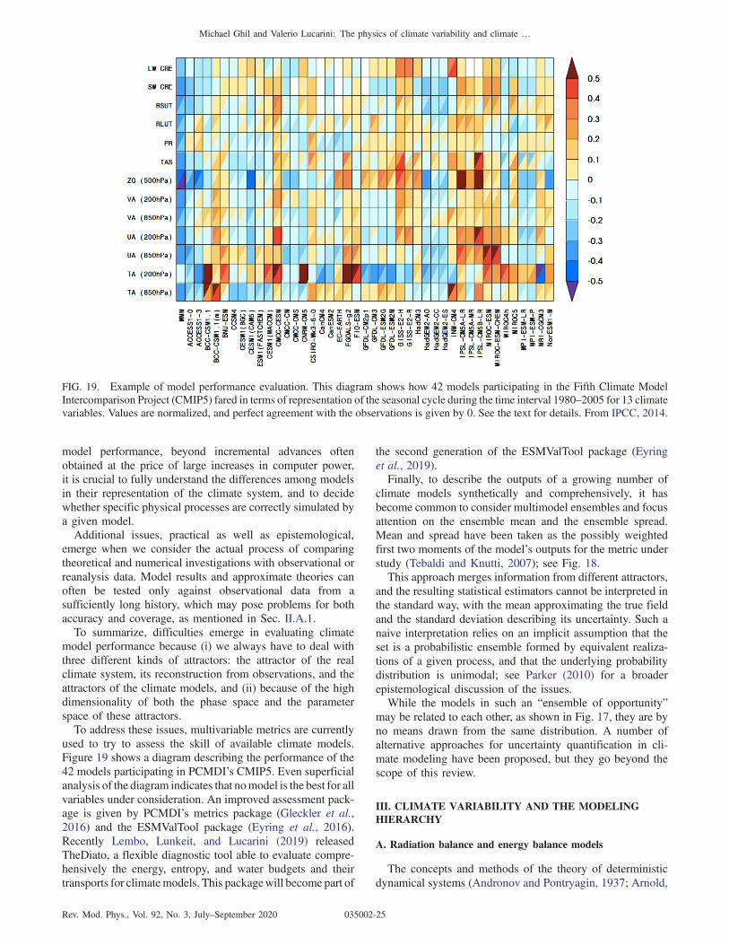
model performance, beyond incremental advances oftenobtained at the price of large increases in computer power,it is crucial to fully understand the differences among modelsin their representation of the climate system, and to decidewhether specific physical processes are correctly simulated bya given model.Additional issues, practical as well as epistemological,

emerge when we consider the actual process of comparingtheoretical and numerical investigations with observational orreanalysis data. Model results and approximate theories canoften be tested only against observational data from asufficiently long history, which may pose problems for bothaccuracy and coverage, as mentioned in Sec. II.A.1.To summarize, difficulties emerge in evaluating climate

model performance because (i) we always have to deal withthree different kinds of attractors: the attractor of the realclimate system, its reconstruction from observations, and theattractors of the climate models, and (ii) because of the highdimensionality of both the phase space and the parameterspace of these attractors.To address these issues, multivariable metrics are currently

used to try to assess the skill of available climate models.Figure 19 shows a diagram describing the performance of the42 models participating in PCMDI’s CMIP5. Even superficialanalysis of the diagram indicates that nomodel is the best for allvariables under consideration. An improved assessment pack-age is given by PCMDI’s metrics package (Gleckler et al.,2016) and the ESMValTool package (Eyring et al., 2016).Recently Lembo, Lunkeit, and Lucarini (2019) releasedTheDiato, a flexible diagnostic tool able to evaluate compre-hensively the energy, entropy, and water budgets and theirtransports for climatemodels. This packagewill become part of

the second generation of the ESMValTool package (Eyringet al., 2019).Finally, to describe the outputs of a growing number of

climate models synthetically and comprehensively, it hasbecome common to consider multimodel ensembles and focusattention on the ensemble mean and the ensemble spread.Mean and spread have been taken as the possibly weightedfirst two moments of the model’s outputs for the metric understudy (Tebaldi and Knutti, 2007); see Fig. 18.This approach merges information from different attractors,

and the resulting statistical estimators cannot be interpreted inthe standard way, with the mean approximating the true fieldand the standard deviation describing its uncertainty. Such anaive interpretation relies on an implicit assumption that theset is a probabilistic ensemble formed by equivalent realiza-tions of a given process, and that the underlying probabilitydistribution is unimodal; see Parker (2010) for a broaderepistemological discussion of the issues.While the models in such an “ensemble of opportunity”

may be related to each other, as shown in Fig. 17, they are byno means drawn from the same distribution. A number ofalternative approaches for uncertainty quantification in cli-mate modeling have been proposed, but they go beyond thescope of this review.

III. CLIMATE VARIABILITY AND THE MODELINGHIERARCHY

A. Radiation balance and energy balance models

The concepts and methods of the theory of deterministicdynamical systems (Andronov and Pontryagin, 1937; Arnold,

FIG. 19. Example of model performance evaluation. This diagram shows how 42 models participating in the Fifth Climate ModelIntercomparison Project (CMIP5) fared in terms of representation of the seasonal cycle during the time interval 1980–2005 for 13 climatevariables. Values are normalized, and perfect agreement with the observations is given by 0. See the text for details. From IPCC, 2014.



1983; Guckenheimer and Holmes, 1983) were first applied tosimple models of atmospheric and oceanic flows, startingabout half a century ago (Stommel, 1961; Lorenz, 1963;Veronis, 1963). More powerful computers now allow theirapplication to fairly realistic and detailed models of theatmosphere, the ocean, and the coupled atmosphere-oceansystem. We start by presenting such a hierarchy of models.This presentation is interwoven with that of the successive

bifurcations that lead from simple to more complex solutionbehavior for each climate model. Useful tools for comparingmodel behavior across the hierarchy and with observationsare provided by ergodic theory (Eckmann and Ruelle, 1985;Ghil, Chekroun, and Simonnet, 2008). Among these tools,advanced methods for the analysis and prediction of univariateand multivariate time series play an important role; see Ghilet al. (2002) and references therein.The concept of a modeling hierarchy in climate dynamics

was introduced by Schneider and Dickinson (1974). Severalother authors have discussed in greater detail the role of such ahierarchy in the understanding and prediction of climatevariability (Ghil and Robertson, 2000; Saltzman, 2001;Lucarini, 2002; Dijkstra and Ghil, 2005; Held, 2005). Atpresent, the best-developed hierarchy is for atmosphericmodels. These models were originally developed for weathersimulation and prediction on a timescale of hours to days.Currently they serve, in a stand-alone mode or coupled tooceanic and other models, to address climate variability on alltimescales.The first rung of the modeling hierarchy for the atmosphere

is formed by zero-dimensional (0D) models, where thenumber of dimensions, from 0 to 3, refers to the number ofindependent space variables used to describe the modeldomain, i.e., to physical-space dimensions. Such 0D modelsessentially attempt to follow the evolution of the globallyaveraged air temperature at surface as a result of changes inglobal radiative balance:

cdTdt

¼ Ri − Ro; ð13aÞ

Ri ¼ μQ0f1 − αðTÞg; ð13bÞ

Ro ¼ σmðTÞðTÞ4: ð13cÞ

Here Ri and Ro are incoming solar radiation and outgoingterrestrial radiation. The heat capacity c is that of the globalatmosphere plus that of the global ocean or some fractionthereof, depending on the timescale of interest: one might onlyinclude in c the ocean mixed layer when interested insubannual timescales, but the entire ocean when studyingpaleoclimate; see, e.g., Saltzman (2001).The rate of change of T with time t is given by dT=dt, while

Q0 is the solar radiation received at the top of the atmosphere,also called the solar constant, σ is the Stefan-Boltzmannconstant, and μ is an insolation parameter equal to unity forpresent-day conditions. To have a closed, self-consistentmodel, the planetary reflectivity or albedo α and graynessfactor m have to be expressed as functions of T; m ¼ 1 for a

perfectly black body and 0 < m < 1 for a gray bodylike Earth.There are two kinds of one-dimensional (1D) atmospheric

models, for which the single spatial variable is latitude orheight, respectively. The former are so-called energy balancemodels (EBMs), which consider the generalization ofmodel (13a) for the evolution of surface air temperatureT ¼ Tðx; tÞ, say,

cðxÞ ∂T∂t ¼ Ri − Ro þD: ð14Þ

The terms Ri and Ro are similar to those given in Eqs. (13b)and (13c) for the 0D case but can now be functions of themeridional coordinate x, latitude, colatitude, or sine oflatitude, as well as of time t and temperature T. The horizontalheat-flux term D describes the convergence of the heattransport across latitude belts; it typically contains first andsecond partial derivatives of T with respect to x, while cðxÞrepresents the system’s space-dependent heat capacity.Thus, Eq. (14) corresponds physically to a nonlinear heat or

reaction-diffusion equation, and mathematically to a nonlinearparabolic PDE. Hence, the rate of change of local temperatureT with respect to time also becomes a partial derivative∂Tðx; tÞ=∂t. Two such models were introduced independentlyby Budyko (1969) in the then Soviet Union and by Sellers(1969) in the United States.The first striking results of theoretical climate dynamics

were obtained in showing that Eq. (14) could have twostable steady-state solutions, depending on the value of theinsolation parameter μ; see Eq. (13b).18

This multiplicity of stable steady states, or physicallypossible stationary climates of our planet, can be explainedin its simplest form by the 0D model of Eq. (13). Notethat the time derivative of the global temperature T inEq. (13a) can be written as minus the derivative of a potentialVðTÞ ¼ −

RfRiðTÞ − RoðTÞgdT, viz., dT=dt¼−dVðTÞ=dT.In the case of bistability, the two local minima of V correspondto the stable solutions, or fixed points, and the local maximumof V corresponds to the unstable solution; see Fig. 20.The physical explanation lies in the fact that for a fairly

broad range of μ values around μ ¼ 1.0 the curves for Ri andRo as a function of T intersect at three points. One of thesepoints corresponds to the present climate (highest T value),and another one corresponds to an ice-covered planet (lowestT value); both are stable, while the third one, i.e., theintermediate T value, is unstable.To obtain this result, it suffices to make two assumptions:

(i) that α ¼ αðTÞ in Eq. (13b) is a piecewise-linear function of

18After the publication of the Budyko (1969) and Sellers (1969)models, it became apparent that massive nuclear explosions couldinduce a nuclear winter: namely, reducing the incoming solarradiation by a dramatic increase in atmospheric particulate mattercould potentially trigger an even greater disaster for life on Earth thannuclear war itself; see, e.g., Turco et al. (1983). Studies to this effectwere influential in reducing the size of nuclear arsenals at the endof the Cold War. Strikingly, the two contributions came almostsimultaneously from scientists belonging to the Cold War’s twoopposing geopolitical blocks.



T, or, more generally, a monotonically increasing one with asingle inflection point, with high albedo at low temperaturedue to the presence of snow and ice, and low albedo at high Tdue to their absence; and (ii) that m ¼ mðTÞ in Eq. (13c) is asmooth, increasing function of T that captures in its simplestform the “greenhouse effect” of trace gases and water vapor.The EBM modelers (Held and Suarez, 1974; North, 1975;

Ghil, 1976) called the ice-covered state a deep freeze. Thepossibility of such a state in Earth’s history was met withconsiderable incredulity by much of the climate communityfor being incompatible with existing paleoclimatic evidence atthe time. Geochemical evidence led in the early 1990s to thediscovery of a snowball or, at least, slush-ball Earth prior tothe emergence of multicellular life, 6 × 108 yr ago (Hoffmanet al., 1998; Hoffman and Schrag, 2002). This discovery didnot lead, however, to more enthusiasm for the theoreticalprediction of such a state almost two decades earlier.The bifurcation diagram of a 1D EBM, like the one of

Eq. (14), is shown in Fig. 21. It displays the model’s meantemperature T as a function of the fractional change μ inthe insolation Q0 ¼ Q0ðxÞ at the top of the atmosphere. TheS-shaped curve in the figure arises from two back-to-backsaddle-node bifurcations. Bensid and Diaz (2019) recentlyprovided a mathematically rigorous treatment of the bifurca-tion diagram of a Budyko-type 1D EBM.The normal form of the first saddle-node bifurcation is

_X ¼ μ − X2: ð15Þ

Here X stands for a suitably normalized form of T and _X is therate of change of X, while μ is a parameter that measures thestress on the system, in particular, a normalized form ofthe insolation parameter in Eq. (13b).The uppermost branch corresponds to the steady-state

solution X ¼ þμ1=2 of Eq. (15), and it is stable. This branchmatches Earth’s present-day climate well for μ ¼ 1.0; moreprecisely the steady-state solution T ¼ Tðx; μÞ of the full 1DEBM (not shown) closely matches the annual mean temper-ature profile from instrumental data over the last century(Ghil, 1976).The intermediate branch starts out at the left as the second

solution X ¼ −μ1=2 of Eq. (15), and it is unstable. It blendssmoothly into the upper branch of a coordinate-shifted andmirror-reflected version of Eq. (15), say,

_X ¼ ðμ − μ0Þ þ ðX − X0Þ2: ð16Þ

This branch X ¼ X0 þ ðμ0 − μÞ1=2 is also unstable. Finally,the lowermost branch in Fig. 21 is the second steady-statesolution of Eq. (16) X ¼ X0 − ðμ0 − μÞ1=2, and it is stable likethe uppermost branch. The lowermost branch correspondsto an ice-covered planet at the same distance from the Sunas Earth.The fact that the upper-left bifurcation point ðμc; TcÞ in

Fig. 21 is so close to present-day insolation values createdgreat concern in the climate dynamics community in the mid1970s, when these results were obtained. Indeed, much moredetailed computations (discussed later) confirmed that areduction of about 2%–5% of insolation values would sufficeto precipitate Earth into a deep freeze. The great distance ofthe lower-right bifurcation point ðμd; TdÞ from present-dayinsolation values, on the other hand, suggests that one wouldhave to nearly double atmospheric opacity, say, for Earth’sclimate to jump back to more comfortable temperatures.These results follow Ghil (1976). Held and Suarez (1974)

and North (1975) obtained similar results, and a detailedcomparison between EBMs appears in Chapter 10 of Ghil andChildress (1987). Ghil (1976) rigorously, then North et al.

snowball warm

V(T)

unstable

T

FIG. 20. Scalar double-well potential function VðTÞ. The warmand “deep-freeze” or snowball states correspond to the system’stwo stable fixed points, separated by an unstable one.

FIG. 21. Bifurcation diagram for the solutions of an energybalance model (EBM), showing the global mean temperature T vsthe fractional change μ of insolation at the top of the atmosphere.The arrows pointing up and down at about μ ¼ 1.4 indicate thestability of the branches: toward a given branch if it is stable andaway from it if it is unstable. The other arrows show the hysteresiscycle that global temperatures would have to undergo fortransition from the upper stable branch to the lower one andback. The angle γ gives the measure of the present climate’ssensitivity to changes in insolation. From Ghil and Childress,1987.



(1979) numerically, pointed out that a double-well potential,like the one sketched in Fig. 20, does exist for higher-dimensional (North et al., 1979) and even infinite-dimensional(Ghil, 1976) versions of an EBM. In higher-dimensionalcases, the maximum of the potential shown in Fig. 20 isreplaced by a saddle, or “mountain pass”; see, e.g., Ghil andChildress (1987), Sec. 10.4. In this case, dimensionality refersto phase space rather than physical space; see Sec. V for amore detailed discussion.

B. Other atmospheric processes and models

The 1D atmospheric models in which the details of radiativeequilibrium are investigated with respect to a height coor-dinate z (geometric height, pressure, etc.) are often calledradiative-convective models (Ramanathan and Coakley,1978). This name emphasizes the key role that convectionplays in vertical heat transfer. While these models historicallypreceded EBMs as rungs on the modeling hierarchy, it wasonly recently shown that they too could exhibit multipleequilibria (Li et al., 1997). The word equilibrium, here and inthe rest of this review, refers simply to a stationary state of themodel rather than a true thermodynamic equilibrium.Two-dimensional (2D) atmospheric models are also of two

kinds, according to the third space coordinate that is notexplicitly included. Models that explicitly resolve two hori-zontal coordinates, on the sphere or on a plane tangent to it,tend to emphasize the study of the dynamics of large-scaleatmospheric motions. They often have a single layer or two.Those that explicitly resolve a meridional coordinate andheight are essentially combinations of EBMs and radiative-convective models and emphasize therewith the thermody-namic state of the system rather than its dynamics.Yet another class of “horizontal” 2Dmodels is the extension

of EBMs to resolve zonal aswell asmeridional surface features,in particular, land-sea contrasts. We see in Sec. III.C.2 howsuch a 2D EBM is used when coupled to an oceanic model.Schneider and Dickinson (1974) and Ghil and Robertson

(2000) discussed additional types of 1D and 2D atmosphericmodels, along with some of their main applications. Finally,to encompass and resolve the main atmospheric phenomenawith respect to all three spatial coordinates, as discussed inSec. II.D, GCMs occupy the pinnacle of the modelinghierarchy; see, e.g., Randall (2000).The mean zonal temperature’s dependence on the insolation

parameter μ, as obtained for 1D EBMs and shown in Fig. 21,was confirmed to the extent possible by using a simplifiedGCM coupled to a “swamp” ocean model (Wetherald andManabe, 1975). More precisely, forward integrations with aGCM cannot confirm the presence of the intermediate,unstable branch. Nor was it possible in the mid 1970s, whenthis numerical experiment was carried out, to reach the deep-freeze stable branch, as it was called at the time, because of theGCM’s computational limitations.Still, the normal form of the saddle-node bifurcation, given

by Eq. (15), suggests a parabolic shape of the upper, present-day-like branch near the upper-left bifurcation point in ourfigure, namely, ðμc; TcÞ. This parabolic shape is characteristicof the dependence of a variable that represents the modelsolution on a parameter that represents the intensity of the

forcing in several types of bifurcations; moreover, this shape isnot limited to the bifurcation’s normal form, like Eqs. (15)and (16), but instead is much more general. The GCMsimulations support quite well a similar shape for the globallyaveraged temperature profiles of the GCM’s five verticallayers; see Wetherald and Manabe (1975), Fig. 5. See thediscussion in Secs. IV.E.5 and V.Ghil and Robertson (2000) also described the separate

hierarchies that have grown over the last quarter century inmodeling the ocean and the coupled ocean-atmospheresystem. More recently an overarching hierarchy of Earthsystem models that encompass all subsystems of interest(atmosphere, biosphere, cryosphere, hydrosphere, and litho-sphere) has been developing. Eventually, the partial resultsabout each subsystem’s variability, outlined in this section andSec. 4, will have to be verified from one rung to the next of thefull Earth system modeling hierarchy.

C. Oscillations in the ocean’s thermohaline circulation

1. Theory and simple models

Historically, the thermohaline circulation (THC) [see, e.g.,Dijkstra and Ghil (2005) and Kuhlbrodt et al. (2007)] was firstamong the climate system’s major processes to be studiedusing a simple mathematical model. Stommel (1961) formu-lated a two-box model and showed that it possesses multipleequilibria.A sketch of the Atlantic Ocean’s THC and its interactions

with the atmosphere and cryosphere on long timescales isshown in Fig. 22. These interactions can lead to climateoscillations with multimillennial periods, such as the Heinrichevents [see, e.g., Ghil (1994) and references therein], and aresummarized in the figure’s caption. An equally schematicview of the global THC is provided by the widely known“conveyor-belt” (Broecker, 1991) diagram. The latter diagramcaptures greater horizontal, 2D detail, but it does not com-monly include the THC’s interactions with water in both itsgaseous and solid phases, which Fig. 22 does include.Basically, the THC is due to denser water sinking, lighter

water rising, and water mass continuity closing the circuitthrough near-horizontal flow between the areas of rising andsinking effects of temperature T and salinity S on the oceanwater’s density ρ ¼ ρðT; SÞ oppose each other: the density ρdecreases as T increases, and it increases as S increases. It isthese two effects that give the thermohaline circulation itsname, from the Greek words for T and S. In high latitudes, ρincreases as the water loses heat to the air above and, if sea iceis formed, as the water underneath is enriched in brine. At lowlatitudes, ρ increases due to evaporation but decreases due tosensible heat flux into the ocean.For the present climate, the temperature effect is stronger

than the salinity effect, and ocean water is observed to sink incertain areas of the high-latitude North Atlantic and SouthernOcean, with limited areas of deep-water formation elsewhere,and to rise everywhere else. Thus, in a thermohaline regime Tis more important than S and hence comes before it.During certain remote geological times, deep water may

have formed in the global ocean near the equator; such anoverturning circulation of opposite sign to that prevailing



today was named halothermal, S before T. The quantificationof the relative effects of T and S on the oceanic water mass’sbuoyancy at high and low latitudes is far from complete,especially for paleocirculations; the association of the latterwith salinity effects that exceed the thermal ones [e.g., duringthe Palaeocene, ≃5.7 × 107 yr ago; see Kennett and Stott(1991)] is thus rather tentative.To study the reversal of the abyssal circulation due to the

opposite effects of T and S, Stommel (1961) considered amodel with two pipes connecting two boxes. He showed thatthe system of two nonlinear, coupled ordinary differentialequations that govern the temperature and salinity differencesbetween the two well-mixed boxes has two stable steady-statesolutions; these two steady states are distinguished by thedirection of flow in the upper and the lower pipe.Stommel was primarily concerned with distinct local con-

vection regimes, and hence vertical stratifications, in the NorthAtlantic and the Mediterranean or the Red Sea, say. Today wemainly think of one box as representing the low latitudes andthe other one the high latitudes in the global THC; seeMarotzke(2000) and references therein. Subsequently, many other THCmodels that used more complex box-and-pipe geometries havebeen proposed and studied; see, e.g., Rooth (1982), Scott,Marotzke, and Stone (1999), Titz et al. (2002), and Lucariniand Stone (2005).The next step in the hierarchical modeling of the THC is

that of 2D meridional-plane models, in which the temperatureand salinity fields are governed by coupled nonlinear PDEswith two independent space variables, say, latitude and depth;see, e.g., Cessi and Young (1992), Quon and Ghil (1992), and

Lucarini, Calmanti, and Artale (2005, 2007). Given boundaryconditions for such a model that are symmetric about theEquator, like the equations themselves, one expects a sym-metric solution, in which water either sinks near the poles andrises everywhere else (thermohaline) or sinks near the Equatorand rises everywhere else (halothermal). These two symmetricsolutions correspond to the two equilibria of the Stommel(1961) two-box model; see Thual and McWilliams (1992) fora discussion of the relationship between 2D and box models.In fact, symmetry breaking can occur, leading gradually

from a symmetric two-cell circulation to an antisymmetricone-cell circulation. In between, all degrees of dominance ofone cell over the other are possible. A situation lying some-where between the two seems to resemble most closely themeridional overturning diagram of the Atlantic Oceanin Fig. 22.The gradual transition is illustrated by Fig. 23, and it can

be described by a pitchfork bifurcation; see Dijkstra andGhil (2005):

_X ¼ fðX; μÞ ¼ μX − X3: ð17ÞHere X measures how asymmetric the solution is, so X ¼ 0 isthe symmetric branch, and μ measures the stress on thesystem, in particular, a normalized form of the buoyancy fluxat the surface. For μ < 0 the symmetric branch is stable, whilefor μ > 0 the two branches X ¼ �μ1=2 inherit its stability.In the 2D THC problem, the left cell dominates on one of

the two branches, while the right cell dominates on the other:for a given value of μ, the two stable steady-state solutions,on the fX ¼ þμ1=2g branch and the fX ¼ −μ1=2g branch,respectively, are mirror images of each other. The idealizedTHC in Fig. 22, with the North Atlantic deep water extendingto the Southern Ocean’s polar front, corresponds to one ofthese two branches. In theory, therefore, a mirror-imagecirculation, with the Antarctic bottom water extending tothe North Atlantic’s polar front, is equally possible.A complementary point of view to the one taken thus far

suggests that surface winds and tides play a major role in thedriving and maintenance of the large-scale ocean circulation(Wunsch, 2002, 2013). In particular, Cessi (2019) argued thatthe meridional overturning is actually powered by momentumfluxes and not buoyancy fluxes. Because of the ongoingarguments on this topic, the THC is increasingly termed themeridional overturning circulation (MOC).

2. Bifurcation diagrams for GCMs

Bryan (1986) was the first to document transition from atwo-cell to a one-cell circulation in a simplified ocean GCMwith idealized, symmetric forcing. In Sec. III.B, atmosphericGCMs essentially confirmed the EBM results. Results ofcoupled ocean-atmosphere GCMs, however, have led toquestions about whether the presence of more than one stableTHC equilibrium is actually realistic. The situation withrespect to the THC’s pitchfork bifurcation (17) is thus subtlerthan it was with respect to Fig. 21 for radiative equilibria.Dijkstra (2007) showed, however, by comparing observa-

tional and reanalysis data with high-end ocean GCMs that theAtlantic Ocean’s current THC is actually in its multiple-equilibria regime. Climate models of intermediate complexity

FIG. 22. Schematic diagram of an Atlantic meridional crosssection from North Pole (NP) to South Pole (SP) showingmechanisms likely to affect the thermohaline circulation(THC) on various timescales. Changes in the radiation balanceRin − Rout are due, at least in part, to changes in extent ofNorthern Hemisphere (NH) snow and ice cover V, and to howthese changes affect the global temperature T; the extent ofSouthern Hemisphere ice is assumed to be constant to a firstapproximation. The change in hydrologic cycle expressed in theterms Prain − Pevap for the ocean and Psnow − Pabl for the snowand ice is due to changes in ocean temperature. Deep-waterformation in the North Atlantic subpolar sea (North Atlantic deepwater, NADW) is affected by changes in ice volume and extentand regulates the intensity C of the THC; changes in Antarcticbottom water (AABW) formation are neglected in this approxi-mation. The THC intensity C in turn affects the system’stemperature and is also affected by it. From Ghil, Mulhaupt,and Pestiaux, 1987.



did indeed find the Atlantic Ocean to be multistable [see, e.g.,Rahmstorf et al. (2005)], while several of the GCMs used inrecent IPCC ARs did not show such a behavior, with anexception coming in the study by Hawkins et al. (2011); seeFig. 24. Thus, a failure of high-end models in the hierarchy toconfirm results obtained on the hierarchy’s lower rungs doesnot necessarily imply that it is the simpler models that arewrong. To the contrary, such a failure might well indicate thatthe high-end models, no matter how detailed, may still berather imperfect; see Ghil (2015) for a summary.Internal variability of the THC, with smaller and more

regular excursions than the large and totally irregular jumpsassociated with bistability, was studied intensively in the late1980s and the 1990s. These studies placed themselves onvarious rungs of the modeling hierarchy, from box models

through 2D models and all the way to ocean GCMs. Asummary of the different kinds of oscillatory variability foundin the latter appears in Table I. Such oscillatory behaviorseems to more closely match the instrumentally recorded THCvariability, as well as the paleoclimatic records for the recentgeological past, than bistability.The (multi)millennial oscillations interact with variability

in the surface features and processes shown in Fig. 22. Chenand Ghil (1996), in particular, studied some of the interactionsbetween atmospheric processes and the THC. They used a so-called hybrid coupled model, namely, a 2D EBM, coupled to arectangular-box version of the North Atlantic rendered by alow-resolution ocean GCM. This hybrid model’s regimediagram is shown in Fig. 25(a). A steady state is stable forhigher values of the coupling parameter λao or of the EBM’s

FIG. 24. Multistability of the THC for (a) Earth models ofintermediate complexity, and (b) an IPCC-class climate model.Parameter controlling the freshwater input in the North Atlanticbasin on the abscissa and the THC’s intensity on the ordinate.(a) From Rahmstorf et al., 2005. (b) From Hawkins et al. (2011).

FIG. 23. Transition from a symmetric to an increasinglyasymmetric meridional ocean circulation. The stream functionplots represent results from an idealized 2D model of thermo-solutal convection in a rectangular domain for a prescribed valueof the Rayleigh number and increasing values of the nondimen-sional intensity γ of the salinity flux at the surface. (a) γ ¼ 0.40.(b) γ ¼ 0.50. (c) γ ¼ 0.55. From Quon and Ghil, 1992.



diffusion parameter d. Interdecadal oscillations with a periodof 40–50 yr are self-sustained and stable for lower values ofthese parameters.The self-sustained THC oscillations in question are

characterized by a pair of vortices of opposite sign thatgrow and decay in quadrature with each other in theocean’s upper layers. Their centers follow each othercounterclockwise through the northwestern quadrant ofthe model’s rectangular domain. Both the period and thespatiotemporal characteristics of the oscillation are thusrather similar to those seen in a fully coupled GCM withrealistic geometry (Delworth, Manabe, and Stouffer, 1993).The transition from a stable equilibrium to a stable limitcycle via Hopf bifurcation in this hybrid coupled modelis shown in Fig. 25(b), and we elaborate upon it inSec. III.D.2.

D. Bistability, oscillations, and bifurcations

In Secs. III.A, III.B, and III.C.1 we introduced bistability ofsteady-state solutions via saddle-node and pitchfork bifurca-tions, while in Sec. III.C.2 we mentioned oscillatory solutions

and Hopf bifurcation as the typical way the latter are reachedas a model parameter changes. We start here by summarizingthe bifurcations of steady-state solutions, often referred to asequilibria, and then introduce and discuss the normal forms ofHopf bifurcation, both supercritical and subcritical.

1. Bistability and steady-state bifurcations

Section III.B introduced EBMs and explained how thepresent climate and a totally ice-covered Earth could result ascoexisting stable steady states over a certain parameter range.The normal forms of a supercritical and a subcritical saddle-node bifurcation were given as Eqs. (15) and (16), respec-tively. Here the criticality is defined as the existence of the twoequilibria, stable and unstable, to the right or the left of thecritical or bifurcation point.An S-shaped bifurcation curve, such as the one that appears

in Fig. 21 for the 1D EBM of Eq. (14), can be obtained easilyby soldering smoothly together the back-to-back saddle-nodebifurcations of Eqs. (15) and (16). While there is no genericnormal form for such a curve, the following is a simpleexample:

TABLE I. Oscillations in the ocean’s thermohaline circulation. Anomalies are defined as the difference between the monthly mean value of avariable and its climatological mean. See also Ghil (1994).

Timescale Phenomena Mechanism

Decadal Local migration of surface anomalies in the northwestcorner of the ocean basin

Localized surface density anomalies due tosurface coupling

Gyre advection in midlatitudes Gyre advectionCentennial Loop-type, meridional circulation Conveyor-belt advection of density anomalies

Millennial Relaxation oscillation, with “flushes” andsuperimposed decadal fluctuations

Bottom water warming due to the strongbraking effect of salinity forcing

FIG. 25. Dependence of THC solutions on two parameters in a hybrid coupled model; the two parameters are the atmosphere-oceancoupling coefficient λao and the atmospheric thermal diffusion coefficient d. (a) Schematic regime diagram. The solid circles stand forthe model’s stable steady states, the open circles stand for stable limit cycles, and the solid curve is the estimated neutral stability curvebetween the former and the latter. (b) Hopf bifurcation curve at fixed d ¼ 1.0 and varying λao; this curve is obtained by fitting a parabolato the model’s numerical-simulation results, shown as filled and open circles. From Chen and Ghil, 1996.



_X ¼ μ − X2; ð18aÞ

_X ¼ ðμ − μ0Þ þ ðX − X0Þ2; ð18bÞ

with μ0 ¼ 1 and X0 ¼ −1=2.Note that both the subcritical and supercritical saddle-

node bifurcations are structurally stable, i.e., they persist asthe system of evolution equations, whether a system ofordinary or partial differential equations, is smoothly per-turbed (Andronov and Pontryagin, 1937; Guckenheimer andHolmes, 1983; Temam, 1997; Arnold, 2003) by a smallamount. This robustness is the reason why saddle-nodebifurcations, and other elementary bifurcations referred toas codimension 1, i.e., depending on a single parameter, likethe Hopf bifurcation, are so important and can, in practice, bea guide through the hierarchy of models, in the climatesciences and elsewhere. A striking example was providedin Sec. III.B for the supercritical saddle-node bifurcationthat can be found in the 3D GCM of Wetherald and Manabe(1975) (Fig. 5 therein), as well as the 1D EBM reproducedin Fig. 21.The next kind of bifurcation that leads to bistability of

stationary states is the pitchfork bifurcation introduced inSec. III.C.1 in connection with the THC, and whose normalform is given by Eq. (17). This bifurcation, however, arisesonly in the presence of a mirror symmetry in the model understudy, as seen in Fig. (23a). One suspects, therefore, that it isnot structurally stable with respect to perturbations of thedynamics that do not preserve this symmetry.A simple example is given by the following perturbed

pitchfork bifurcation:

_X ¼ fðX; μ; ϵÞ ¼ Xðμ − X2Þ þ ϵ; ð19Þwhere ϵ is a small parameter. The bifurcation diagrams forϵ ¼ 0 and þ0.1 are given in Figs. 26(a) and 26(b), respec-tively. A nonzero value of ϵ breaks the X → −X symmetry ofEq. (17) since it is no longer the case that fðXÞ ¼ fð−XÞ.Hence, the pitchfork breaks up into a continuous uppermostbranch that is stable for all X values, and a supercriticalsaddle-node bifurcation whose lower branch is stable. Ifϵ < 0, it will be the lowermost branch that is stable for allX values (not shown), and the upper branch of the saddle-nodebifurcation above it that is stable. In both cases, above acritical value associated with the saddle-node bifurcation threesolution branches exist, with the middle one that is unstableand the other two that are stable.One way that the symmetric pitchfork bifurcation present in

2D models of the THC can be broken, as illustrated in Fig. 26,is simply by considering 3D models with zonally asymmetricbasin boundaries. Perturbed pitchfork bifurcations were alsofound in shallow-water models of the wind-driven oceancirculation; see, e.g., Jiang, Jin, and Ghil (1995), Speich,Dijkstra, and Ghil (1995b), and Ghil (2017).

2. Oscillatory instabilities and Hopf bifurcations

In spite of the considerable detail and 3D character ofthe ocean GCM involved in the hybrid coupled model ofChen and Ghil (1996), it is clear that the numericallyobtained bifurcation diagram in Fig. 25(b) is of a simple,

fundamental type. The normal form of such a Hopf bifurcationis given by

_z ¼ ðμþ iωÞzþ cðzzÞz; ð20Þ

where z ¼ xþ iy is a complex variable, while c and ω arenon-negative and μ is a real parameter. For small z, Eq. (20)describes a rotation in the complex plane with an increasingradius jzj when μ > 0, i.e., it contains the possibility of anoscillatory instability, while the cubic term corresponds toan increasing modification of this simple rotation away fromthe origin.The previous parsimonious complex notation follows

Arnold (1983) and Ghil and Childress (1987) and is more

FIG. 26. Bifurcation diagram of the pitchfork bifurcation inEq. (19) (a) for ϵ ¼ 0, and (b) for ϵ ¼ 0.1. Solid lines indicatestable solutions, and dashed lines indicate unstable ones. FromDijkstra and Ghil, 2005.



suggestive and transparent than the more common one thatseparately uses the two real variables x and y; see, e.g.,Guckenheimer and Holmes (1983). The advantages of theformer are apparent when introducing polar variables viaz ¼ ρ1=2eiθ, with ρ ¼ zz ≥ 0. One can then separate the flowinduced by Eq. (20) into a constant rotation with angularvelocity ω and a radius r ¼ ρ1=2 that either increases ordecreases as _ρ≷0 according to

_ρ ¼ 2ρðμþ cρÞ; ð21aÞ

_θ ¼ ω: ð21bÞ

Equation (21a) is quadratic in ρ and has the two rootsρ ¼ 0 and −μ=c. The former corresponds to a fixed point atthe origin z ¼ 0 in Eq. (20), while the latter exists onlywhen cμ < 0.We thus anticipate a solution that is a circle with radius

r ¼ ð−μ=cÞ1=2 when cμ ≠ 0 and the two parameters haveopposite signs. The simpler case is that of the nonzero radiigiven by Eq. (21a) for positive stability parameter μ andnegative saturation parameter c: it corresponds to the super-critical Hopf bifurcation sketched in Fig. 27(a). In this case,the stable fixed point at the origin loses its stability as μchanges sign and transmits it to a limit cycle of parabolicallyincreasing radius.The opposite case of c > 0 is plotted in Fig. 27(b): it

corresponds to subcritical Hopf bifurcation. Here, in fact, thestability of the fixed point is also lost at μ ¼ 0 but there is nooscillatory solution for μ > 0 at all since the higher-orderterms in either Eq. (20) or Eq. (21a) cannot stabilize thelinearly unstable oscillatory solution, which spirals out toinfinity. It is not just that the parabolas in Figs. 27(a) and 27(b)point in opposite directions, as for the saddle-node bifurca-tions in Eqs. (18a) and (18b) or Eqs. (15) and (16), but the twofigures are topologically distinct.

E. Main modes of variability

The atmosphere, ocean, and the coupled ocean-atmosphereclimate system have many modes of variability, as initiallydiscussed in Secs. II.A–II.C. We review here some of the mostimportant ones and comment on the general features ofsuch modes.

1. Modes of variability and extended-range prediction

Several large-scale spatial patterns of atmospheric covari-ability have been studied, starting in the second half of the19th century. Lorenz (1967) and Wallace and Gutzler (1981)provided good reviews of the earlier studies. The earliestwork tended to emphasize “centers of action,” where thevariability is strongest (Teisserenc de Bort, 1881), whilemore recently, it is so-called teleconnections between suchcenters of action that have been emphasized. J. Namias(1910–1997) played a key role in developing the interest insuch teleconnections by applying systematically the useof their spatiotemporal properties to the development ofoperational extended-range weather forecasting; see, e.g.,Namias (1968).Returning to the discussion of prediction in Sec. II.D, it is

important to recall John Von Neumann’s (1903–1957) impor-tant distinction (Von Neumann, 1960) between weather andclimate prediction. To wit, short-term NWP is the easiest,i.e., it is a pure initial-value problem. Long-term climateprediction is next easiest, it corresponds to studying thesystem’s asymptotic behavior, while intermediate-term pre-diction is hardest: both initial and boundary values areimportant. Von Neumann’s role in solving the NWP problemby integrating the discretized equations that govern large-scaleatmospheric motions (Bjerknes, 1904; Richardson, 1922;Charney, Fjørtoft, and Von Neumann, 1950) is well known.In fact, he also played a key role in convening the conferenceon the Dynamics of Climate that was held at Princeton’s

FIG. 27. Bifurcation diagram of the Hopf bifurcation in Eq. (20). (a) Supercritical Hopf bifurcation for c ¼ −1. (b) Subcritical Hopfbifurcation for c ¼ þ1. Solid lines indicate stable solutions (s), and dashed lines indicate unstable ones (u); it is common to plotjzj ¼ −μ1=2 along with jzj ¼ μ1=2 to emphasize that one is actually projecting onto the ðjzj; μÞ plane a paraboloid-shaped, one-parameterfamily of limit cycles with given r ¼ jzj ¼ μ1=2 and 0 ≤ θ < 2π. From Ghil and Childress, 1987.



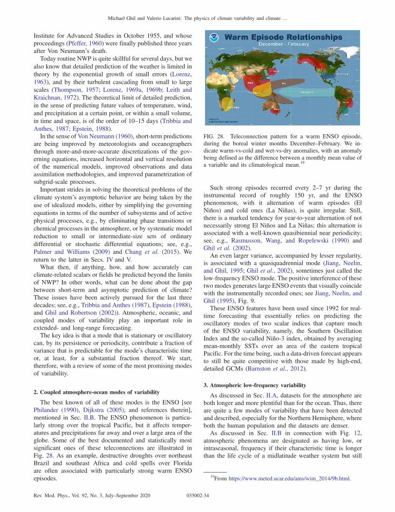
Institute for Advanced Studies in October 1955, and whoseproceedings (Pfeffer, 1960) were finally published three yearsafter Von Neumann’s death.Today routine NWP is quite skillful for several days, but we

also know that detailed prediction of the weather is limited intheory by the exponential growth of small errors (Lorenz,1963), and by their turbulent cascading from small to largescales (Thompson, 1957; Lorenz, 1969a, 1969b; Leith andKraichnan, 1972). The theoretical limit of detailed prediction,in the sense of predicting future values of temperature, wind,and precipitation at a certain point, or within a small volume,in time and space, is of the order of 10–15 days (Tribbia andAnthes, 1987; Epstein, 1988).In the sense of Von Neumann (1960), short-term predictions

are being improved by meteorologists and oceanographersthrough more-and-more-accurate discretizations of the gov-erning equations, increased horizontal and vertical resolutionof the numerical models, improved observations and dataassimilation methodologies, and improved parametrization ofsubgrid-scale processes.Important strides in solving the theoretical problems of the

climate system’s asymptotic behavior are being taken by theuse of idealized models, either by simplifying the governingequations in terms of the number of subsystems and of activephysical processes, e.g., by eliminating phase transitions orchemical processes in the atmosphere, or by systematic modelreduction to small or intermediate-size sets of ordinarydifferential or stochastic differential equations; see, e.g.,Palmer and Williams (2009) and Chang et al. (2015). Wereturn to the latter in Secs. IV and V.What then, if anything, how, and how accurately can

climate-related scalars or fields be predicted beyond the limitsof NWP? In other words, what can be done about the gapbetween short-term and asymptotic prediction of climate?These issues have been actively pursued for the last threedecades; see, e.g., Tribbia and Anthes (1987), Epstein (1988),and Ghil and Robertson (2002)). Atmospheric, oceanic, andcoupled modes of variability play an important role inextended- and long-range forecasting.The key idea is that a mode that is stationary or oscillatory

can, by its persistence or periodicity, contribute a fraction ofvariance that is predictable for the mode’s characteristic timeor, at least, for a substantial fraction thereof. We start,therefore, with a review of some of the most promising modesof variability.

2. Coupled atmosphere-ocean modes of variability

The best known of all of these modes is the ENSO [seePhilander (1990), Dijkstra (2005), and references therein],mentioned in Sec. II.B. The ENSO phenomenon is particu-larly strong over the tropical Pacific, but it affects temper-atures and precipitations far away and over a large area of theglobe. Some of the best documented and statistically mostsignificant ones of these teleconnections are illustrated inFig. 28. As an example, destructive droughts over northeastBrazil and southeast Africa and cold spells over Floridaare often associated with particularly strong warm ENSOepisodes.

Such strong episodes recurred every 2–7 yr during theinstrumental record of roughly 150 yr, and the ENSOphenomenon, with it alternation of warm episodes (ElNiños) and cold ones (La Niñas), is quite irregular. Still,there is a marked tendency for year-to-year alternation of notnecessarily strong El Niños and La Niñas; this alternation isassociated with a well-known quasibiennial near periodicity;see, e.g., Rasmusson, Wang, and Ropelewski (1990) andGhil et al. (2002).An even larger variance, accompanied by lesser regularity,

is associated with a quasiquadrennial mode (Jiang, Neelin,and Ghil, 1995; Ghil et al., 2002), sometimes just called thelow-frequency ENSO mode. The positive interference of thesetwo modes generates large ENSO events that visually coincidewith the instrumentally recorded ones; see Jiang, Neelin, andGhil (1995), Fig. 9.These ENSO features have been used since 1992 for real-

time forecasting that essentially relies on predicting theoscillatory modes of two scalar indices that capture muchof the ENSO variability, namely, the Southern OscillationIndex and the so-called Niño-3 index, obtained by averagingmean-monthly SSTs over an area of the eastern tropicalPacific. For the time being, such a data-driven forecast appearsto still be quite competitive with those made by high-end,detailed GCMs (Barnston et al., 2012).

3. Atmospheric low-frequency variability

As discussed in Sec. II.A, datasets for the atmosphere areboth longer and more plentiful than for the ocean. Thus, thereare quite a few modes of variability that have been detectedand described, especially for the Northern Hemisphere, whereboth the human population and the datasets are denser.As discussed in Sec. II.B in connection with Fig. 12,

atmospheric phenomena are designated as having low, orintraseasonal, frequency if their characteristic time is longerthan the life cycle of a midlatitude weather system but still

FIG. 28. Teleconnection pattern for a warm ENSO episode,during the boreal winter months December–February. We in-dicate warm-vs-cold and wet-vs-dry anomalies, with an anomalybeing defined as the difference between a monthly mean value ofa variable and its climatological mean.19

19From https://www.meted.ucar.edu/ams/wim_2014/9b.html.



https://www.meted.ucar.edu/ams/wim_2014/9b.html





shorter than a season. We are thus discussing here intrinsicvariability, as opposed to the externally forced seasonal cycle,with the latter being easier to understand. More recently oneis also referring to this variability as subseasonal; see, e.g.,Robertson and Vitart (2018).There are essentially two approaches for describing this

intrinsic subseasonal variability: (i) episodic or intermittent,and (ii) oscillatory. The two approaches are complementary,as we shall see, and they have been named the particle andwave descriptions by a crude analogy with quantum mechan-ics (Ghil and Robertson, 2002); see also Sec. I.AThe key ingredient of the particle approach is provided by

so-called persistent anomalies or regimes. The best knownamong these are blocking and zonal flows, which werementioned in Sec. II.B. Other well-known persistent features,especially during boreal winter, are the positive and negativephases of the North Atlantic Oscillation (NAO) and the PacificNorth American (PNA) pattern. A rich literature exists on thereliable identification, description, and modeling of thesepatterns; see Ghil et al. (2019) and references therein. Inthe Southern Hemisphere, there has also been some interest inan approximate counterpart of the PNA called the PacificSouth American (PSA) pattern (Mo and Ghil, 1987).The key ingredient of the wave approach is provided by

oscillatory modes that do not necessarily possess exactperiodicities, but instead the broad spectral peaks that wereillustrated in Fig. 12 and discussed to some extent in Sec. II.B.Probably the best known example of this type in thesubseasonal band is the Madden-Julian oscillation (MJO)(Madden and Julian, 1971). It has a near periodicity of roughly50 days and affects winds and precipitation in the Tropics,being strongest in the Indo-Pacific sector. Like the muchlower-frequency ENSO phenomenon, important extratropicaleffects have been documented; see, e.g., Maloney andHartmann (2000).In spite of the considerable amount of observational,

theoretical, and modeling work dedicated to the MJO, it isstill incompletely understood and not well simulated orpredicted. Some of the reasons for these difficulties includethe key role played in its mechanism by transitions amongliquid and gaseous phases of water in tropical clouds, itsmultiscale character, and the pronounced interactions with theocean (Zhang, 2005).Two extratropical modes in the subseasonal band are the

Branstator-Kushnir wave (Branstator, 1987; Kushnir, 1987)and the 40-day mode associated with the topographic insta-bility first described by Charney and DeVore (1979) in a low-order model. The Branstator-Kushnir wave is, like the MJO,an eastward-traveling wave, while the 40-day mode is astanding wave anchored by the topography.Charney and DeVore (1979) emphasized the bimodality of

the solutions of a model version with only three Fouriermodes, with one stable steady state being zonal and the otherbeing blocked, and did not pursue further the fact that in amore highly resolved version of the model oscillatory solu-tions did appear. Legras and Ghil (1985), Ghil and Childress(1987), and Jin and Ghil (1990) did clarify the role of thehigher meridional modes in the Hopf bifurcation that givesrise to the oscillatory solutions. The potential role of theseresults in the controversy surrounding the effect of

anthropogenic polar amplification on blocking frequencywas mentioned in Sec. II.B.2.While midlatitude weather systems, like tropical ones,

involve precipitation, their large-scale properties seem to bemuch less affected by wet processes; the former ariseessentially from purely dynamical as opposed to largelythermodynamical mechanisms. For simplicity, we thus tryto illustrate in further detail the complementarity of the waveand particle approaches for the extratropical topographicoscillation.Given the recent interest in the physical literature for

synchronization in continuous media [see Duane et al.(2017) and references therein], it might be a challengingnotion for this readership that one can accommodate in a fairlynarrow frequency band, between roughly 0.1 and 0.01 day−1,three distinct oscillatory modes that do not seem to synchron-ize: in the Tropics the MJO, with a period of ≃50 days, and inmidlatitudes the Branstator-Kushnir wave, with a period of≃30 days, along with the topographic oscillatory mode, with aperiod of ≃40 days; see, for instance, Dickey, Ghil, andMarcus (1991), Fig. 11. Not only are these three frequenciesfairly close, i.e., the detuning is fairly small, but the character-istic wavelengths of all three of these oscillatory modes arequite large with respect to the radius of Earth, and severalteleconnections mentioned so far extend across continents andoceans; see Fig. 28.Let us now concentrate on the topographic wave mode

and its relationship with the blocking and zonal particles.Ghil et al. (2019) reviewed the evidence provided by ahierarchy of models for the presence of a Hopf bifurcationthat arises from the interaction of the large-scale westerlyflow in midlatitudes with the topography of the NorthernHemisphere.Certain spatial features of the phases of this mode do

present striking similarities to the blocked and zonal flows thatappear not just as the two stable equilibria in the highlyidealized model of Charney and DeVore (1979) but also asunstable, though long-lived, patterns in much more realisticmodels, like the three-level quasigeostrophic (QG3) modeloriginally formulated by Marshall and Molteni (1993). Thelatter model is still widely used to study the nonlineardynamics of large-scale, midlatitude atmospheric flows;see, e.g., Kondrashov, Ide, and Ghil (2004) and Lucariniand Gritsun (2020).We summarize here the relevant conclusions of the Ghil

et al. (2019) review on the observational, theoretical, andmodeling literature of multiple regimes and oscillatory modesof subseasonal variability. Four complementary approaches toexplaining this variability are illustrated in Fig. 29.One approach to persistent anomalies in midlatitude atmos-

pheric flows on subseasonal timescales is to consider themsimply as due to a slowing down of Rossby waves or theirlinear interference (Lindzen, 1986). This approach is illus-trated in Fig. 29(c): zonal flow Z and blocked flow B aresimply slow phases of an harmonic oscillation, like theneighborhood of t ¼ π=2 or 3π=2 for a sine wave sinðtÞ;otherwise, they are due to an interference of two or more linearwaves, like the one occurring for a sum A sinðtÞ þ B sinð3tÞnear t ¼ ð2kþ 1Þπ=2. A more ambitious, quasilinear version



of this approach is to study long-lived resonant wave triadsbetween a topographic Rossby wave and two free Rossbywaves (Egger, 1978; Trevisan and Buzzi, 1980; Ghil andChildress, 1987). Neither version of this line of thought,though, explains the organization of the persistent anomaliesinto distinct flow regimes.Rossby (1939) initiated a different, genuinely nonlinear

approach by suggesting that multiple equilibria may explainpreferred atmospheric flow patterns. They drew an analogybetween such equilibria and hydraulic jumps, and formulatedsimple models in which similar transitions between fasterand slower atmospheric flows could occur. This multiple-equilibria approach was then pursued vigorously in the 1980s(Charney and DeVore, 1979; Charney, Shukla, and Mo, 1981;Legras and Ghil, 1985; Ghil and Childress, 1987), and it isillustrated in Fig. 29(a): one version of the sketch illustratesmodels that concentrated on the B-Z dichotomy (Charney andDeVore, 1979; Charney, Shukla, and Mo, 1981; Benzi et al.,1986), the other on models [see, e.g., Legras and Ghil (1985)]that allowed for the presence of additional clusters, found byKimoto and Ghil (1993a) and Smyth, Ide, and Ghil (1999)among others in observations. The latter include oppositephases of the NAO and PNA anomalies [PNA, RNA, andBNAO in Fig. 29(a)]. The LFV dynamics in this approach isgiven by the preferred transition paths between the two ormore regimes; see Table 1 in Ghil et al. (2019) and referencestherein.A third approach is associated with the idea of oscillatory

instabilities of one or more of the multiple fixed points thatcan play the role of regime centroids. Thus, Legras and Ghil(1985) found a 40-day oscillation arising by Hopf bifurcationoff their blocked regime B, as illustrated in Fig. 29(b).An ambiguity arises, though, between this point of view

and the complementary possibility that the regimes are justslow phases of such an oscillation, caused itself by theinteraction of the midlatitude jet with topography that givesrise to a supercritical Hopf bifurcation. Thus, Kimoto and Ghil(1993a, 1993b) found in their observational data closed pathswithin a Markov chain whose states resembled well-knownphases of an intraseasonal oscillation. Such a possibility wasconfirmed in the QG3 model by Kondrashov, Ide, and Ghil(2004). Furthermore, multiple regimes and intraseasonal

oscillations can coexist in a two-layer model on the spherewithin the scenario of “chaotic itinerancy” (Itoh and Kimoto,1996, 1997).Lucarini and Gritsun (2020) observed that blockings occur

when the system’s trajectory is in the neighborhood of aspecific class of unstable periodic orbits (UPOs). UPOs ingeneral are natural modes of variability that cover a chaoticsystem’s attractor (Cvitanović, 1988; Cvitanovíc andEckhardt, 1991). Here the UPOs that correspond to blockingshave a higher degree of instability than UPOs associated withzonal flow; thus, blockings are associated with anomalouslyunstable atmospheric states, as suggested theoretically byLegras and Ghil (1985) and confirmed experimentally byWeeks et al. (1997). Different regimes may be associated withdifferent bundles of UPOs, a conjecture that could also explainthe efficacy of Markov chains in describing the transitionsbetween qualitatively different regimes.Figure 29(d) refers to the role of stochastic processes in S2S

variability and prediction, whether it be noise that is white intime, as in Hasselmann (1976) or in linear inverse models(Penland, 1989, 1996; Penland and Ghil, 1993; Penland andSardeshmukh, 1995), or red in time, as in certain nonlineardata-driven models (Kravtsov, Kondrashov, and Ghil, 2005,2009; Kondrashov, Kravtsov, and Ghil, 2006; Kondrashovet al., 2013; Kondrashov, Chekroun, and Ghil, 2015) or evennon-Gaussian ones (Sardeshmukh and Penland, 2015).Stochastic processes may enter into models situated on variousrungs of the modeling hierarchy, from the simplest conceptualmodels to high-resolution GCMs. In the former, they mayenter via stochastic forcing, whether additive or multiplicative,Gaussian or not [see, e.g., Kondrashov, Chekroun, and Ghil(2015)], while in the latter they may enter via stochasticparametrizations of subgrid-scale processes; see, e.g., Palmerand Williams (2009) and references therein.Figure 29 summarizes some of the key dynamical mech-

anisms of midlatitude subseasonal variability, as discussed inthis section and in Ghil et al. (2019), without attempting toprovide a definitive answer as to which approach to modelingand prediction of this variability will be the most productive inthe near future.

F. Internal variability and routes to chaos

In this section, we illustrate the wind-driven ocean circu-lation a sequence of successive bifurcations that lead from ahighly symmetric, steady-state circulation to much morefinely structured, irregular, possibly chaotic oscillations.Various issues arise in pursuing such a bifurcation sequenceacross a hierarchy of models and on to the observational data.Midlatitude oceanic gyres appear clearly in Fig. 30 in the

four major extratropical ocean basins, namely, the North andSouth Atlantic and the North and South Pacific. The largesubtropical ocean gyres are formed by a poleward-flowingwestern boundary current, an equatorward-flowing easternboundary current, and the roughly zonally flowing currentsthat connect these two coastal currents off the equator and onthe poleward basin side, respectively. These gyres are char-acterized by so-called anticyclonic rotation, clockwise in theNorthern Hemisphere and counterclockwise in the SouthernHemisphere. In the North Pacific and the North Atlantic, they

(d) Red noise

(a)

(b) (c)

FIG. 29. Schematic overview of atmospheric low-frequencyvariability (LFV) mechanisms; see the text for details. FromGhil et al., 2019.



are accompanied by smaller, cyclonically rotating gyres, whilein the Southern Hemisphere such subpolar gyres are missingand replaced by the Antarctic Circumpolar Current (ACC).The basic phenomenology of these gyres and the detailed

physical mechanisms that give rise to it were described inseveral books [see, e.g., Sverdrup, Johnson, and Fleming(1946), Gill (1982), Ghil and Childress (1987), Pedlosky(1996), Vallis (2006), and Cushman-Roisin and Beckers(2011)] and review papers (Dijkstra and Ghil, 2005; Ghil,2017). The sharp western boundary currents, like the GulfStream in the North Atlantic, the Kuroshio and its cross-basinextension in the North Pacific, and the Brazil Current in theSouth Atlantic, as well as the more diffuse eastern boundarycurrents, like the Canaries Current in the North Atlantic andthe California and Peru currents in the North and SouthPacific, respectively, play a major role in carrying heatpoleward and colder waters equatorward. Hence, these gyres’interannual and interdecadal variability is a major contributorto climate variability.To illustrate the bifurcation sequence that might lead to this

oceanic LFV, we use a highly idealized model of the wind-driven double-gyre circulation in a rectangular geometry. Notethat the counterparts of synoptic weather systems in the oceanare eddies and meanders that have much shorter spatial scalesthan in the atmosphere, but considerably longer timescales:Oð100Þ km in the ocean versus Oð1000Þ km in the atmos-phere, but of the order of several months in time versus of theorder of merely several days. Thus, the definition we used forLFV in the atmosphere (see Sec. III.E.3) corresponds in theocean to a timescale of years to decades.

1. A simple model of the double-gyre circulation

The simplest model that includes several of the mostpertinent mechanisms described in Sec. II.B is governed bythe barotropic quasigeostrophic equations. We consider anidealized, rectangular basin geometry and simplified forcing

that mimics the distribution of vorticity due to the wind stresssketched by Simonnet, Ghil, and Dijkstra (2005) in theirFig. 2. In this idealized model, the amounts of subpolar andsubtropical vorticity injected into the basin are equal and therectangular domain Ω ¼ ð0; LxÞ × ð0; LyÞ is symmetric aboutthe axis of zero wind-stress curl y ¼ Ly=2.The barotropic 2D quasigeostrophic equations in this

idealized setting are

∂tqþ Jðψ ; qÞ − νΔ2ψ þ μΔψ ¼ −τ sin�2πyLy

�; ð22aÞ

q ¼ Δψ − λ−2R ψ þ βy: ð22bÞ

Here x points east and y points north, while q and ψare the potential vorticity and the stream function, respec-tively, and the Jacobian J gives the advection of potentialvorticity by the flow, as discussed in Sec. II.C.3, so Jðψ ; qÞ ¼ψxqy − ψyqx ¼ u · ∇q.The physical parameters are the strength of the planetary

vorticity gradient β ¼ ∂f=∂y, the Rossby radius of deforma-tion λ−2R , the eddy-viscosity coefficient ν, the bottom frictioncoefficient μ, and the wind-stress intensity τ. One considershere free-slip boundary conditions ψ ¼ Δ2ψ ¼ 0; the quali-tative results described later do not depend on the choice ofhomogeneous boundary condition (Jiang, Jin, and Ghil, 1995;Dijkstra and Ghil, 2005).The nonlinear system of PDEs (22) is an infinite-

dimensional dynamical system, and one can thus study itsbifurcations as the parameters change. Two key parameters arethe wind-stress intensity τ and the eddy viscosity ν: as τincreases, the solutions become rougher, while an increase in νrenders them smoother.An important property of Eq. (22) is its mirror symmetry

along the y ¼ Ly=2 axis. This symmetry can be expressed asinvariance with respect to the discrete Z2 group S,

FIG. 30. A map of the main oceanic currents: warm currents in red and cold ones in blue. From Ghil, Chekroun, and Simonnet, 2008.



S½ψðx; yÞ� ¼ −ψðx; Ly − yÞ.

Any solution of Eq. (22) is thus accompanied by its mirror-conjugated solution. Hence, the prevailing bifurcations are ofeither the symmetry-breaking or the Hopf type.

2. Bifurcations in the double-gyre problem

The development of a comprehensive nonlinear theory ofthe double-gyre circulation over the last two decades has gonethrough four main steps. These four steps can be followedthrough the bifurcation tree in Fig. 31.

a. Symmetry-breaking bifurcation

The “trunk” of the bifurcation tree is plotted as the solidblue line in the lower part of Fig. 31. When the forcing τ isweak or the dissipation ν is large, there is only one steadysolution, which is antisymmetric with respect to the midaxis ofthe basin. This solution exhibits two large gyres, along withtheir β-induced western boundary currents. Away from thewestern boundary, such a near-linear solution (not shown) isdominated by so-called Sverdrup balance between wind-stress

curl and the meridional mass transport (Sverdrup, 1947;Gill, 1982).The first generic bifurcation of this quasigeostrophic model

was found to be a genuine pitchfork bifurcation that breaks thesystem’s symmetry as the nonlinearity becomes large enoughwith increasing wind-stress intensity τ (Cessi and Ierley, 1995;Jiang, Jin, and Ghil, 1995). As τ increases, the near-linearSverdrup solution that lies along the solid blue line in thefigure develops an eastward jet along the midaxis, whichpenetrates farther into the domain and also forms two intenserecirculation vortices, on either side of the jet and near thewestern boundary of the domain.The resulting more intense and hence more nonlinear

solution is still antisymmetric about the midaxis, but it losesits stability for some critical value of the wind-stress intensityτ ¼ τp. This value is indicated by the solid square on thesymmetry axis of Fig. 31 and is labeled “Pitchfork” in thefigure.A pair of mirror-symmetric solutions emerges and it is

plotted as the two red solid lines in the figure’s middle part.The stream function fields associated with the two stablesteady-state branches have a rather different vorticity dis-tribution, and they are plotted in the two small panels in theupper left and upper right of Fig. 31. In particular, the jet insuch a solution exhibits a large, stationary meander, rem-iniscent of the semipermanent one that occurs in the GulfStream, just downstream of Cape Hatteras. These asym-metric flows are characterized by one recirculation vortexbeing stronger in intensity than the other; accordingly, theeastward jet is deflected either to the southeast, as isthe case in the observations for the North Atlantic, or tothe northeast.

b. Gyre modes

The next step in the theoretical treatment of the problemwas taken in part concurrently with the first one htat wementioned (Jiang, Jin, and Ghil, 1995) and in part shortlythereafter (Speich, Dijkstra, and Ghil, 1995a; Dijkstra andKatsman, 1997; Sheremet, Ierley, and Kamenkovich,1997). It involved the study of time-periodic instabilitiesthat arise through Hopf bifurcation from either an anti-symmetric or an asymmetric steady flow. Some of thesestudies treated wind-driven circulation models limited to astand-alone, single gyre (Pedlosky, 1996; Sheremet, Ierley,and Kamenkovich, 1997); such a model concentrates onthe larger subtropical gyre while neglecting the smallersubpolar one.The overall idea was to develop a full generic picture of the

time-dependent behavior of the solutions in more turbulentregimes by classifying the various instabilities in a compre-hensive way. However, it quickly appeared that a particularkind of instability leads to so-called gyre modes (Jiang, Jin,and Ghil, 1995; Speich, Dijkstra, and Ghil, 1995a) and wasprevalent across the full hierarchy of models of the double-gyre circulation; furthermore, this instability triggers thelowest nonzero frequency present in all such models(Dijkstra, 2005; Dijkstra and Ghil, 2005).These gyre modes always appear after the first pitchfork

bifurcation, and it took several years to understand their

FIG. 31. Generic bifurcation diagram for the barotropic quasi-geostrophic model of the double-gyre problem: the asymmetry ofthe solution is plotted versus the intensity of the wind stress τ.The stream function field is plotted for a steady-state solutionassociated with each of the three branches; positive values are inred and negative ones are in blue. From Simonnet, Ghil, andDijkstra, 2005.



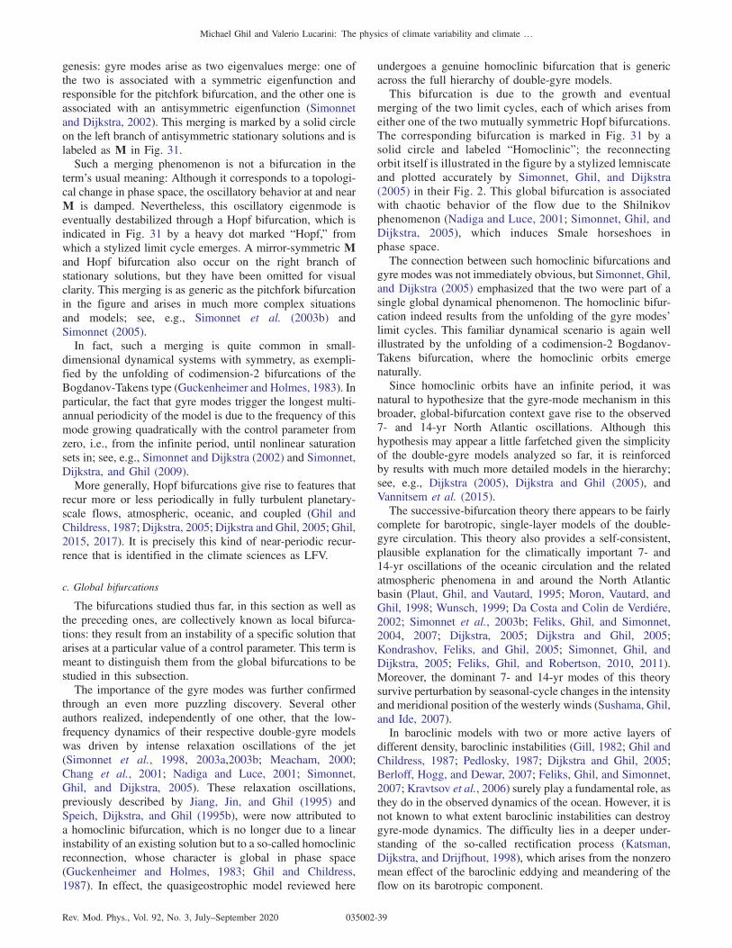
genesis: gyre modes arise as two eigenvalues merge: one ofthe two is associated with a symmetric eigenfunction andresponsible for the pitchfork bifurcation, and the other one isassociated with an antisymmetric eigenfunction (Simonnetand Dijkstra, 2002). This merging is marked by a solid circleon the left branch of antisymmetric stationary solutions and islabeled as M in Fig. 31.Such a merging phenomenon is not a bifurcation in the

term’s usual meaning: Although it corresponds to a topologi-cal change in phase space, the oscillatory behavior at and nearM is damped. Nevertheless, this oscillatory eigenmode iseventually destabilized through a Hopf bifurcation, which isindicated in Fig. 31 by a heavy dot marked “Hopf,” fromwhich a stylized limit cycle emerges. A mirror-symmetric Mand Hopf bifurcation also occur on the right branch ofstationary solutions, but they have been omitted for visualclarity. This merging is as generic as the pitchfork bifurcationin the figure and arises in much more complex situationsand models; see, e.g., Simonnet et al. (2003b) andSimonnet (2005).In fact, such a merging is quite common in small-

dimensional dynamical systems with symmetry, as exempli-fied by the unfolding of codimension-2 bifurcations of theBogdanov-Takens type (Guckenheimer and Holmes, 1983). Inparticular, the fact that gyre modes trigger the longest multi-annual periodicity of the model is due to the frequency of thismode growing quadratically with the control parameter fromzero, i.e., from the infinite period, until nonlinear saturationsets in; see, e.g., Simonnet and Dijkstra (2002) and Simonnet,Dijkstra, and Ghil (2009).More generally, Hopf bifurcations give rise to features that

recur more or less periodically in fully turbulent planetary-scale flows, atmospheric, oceanic, and coupled (Ghil andChildress, 1987; Dijkstra, 2005; Dijkstra and Ghil, 2005; Ghil,2015, 2017). It is precisely this kind of near-periodic recur-rence that is identified in the climate sciences as LFV.

c. Global bifurcations

The bifurcations studied thus far, in this section as well asthe preceding ones, are collectively known as local bifurca-tions: they result from an instability of a specific solution thatarises at a particular value of a control parameter. This term ismeant to distinguish them from the global bifurcations to bestudied in this subsection.The importance of the gyre modes was further confirmed

through an even more puzzling discovery. Several otherauthors realized, independently of one other, that the low-frequency dynamics of their respective double-gyre modelswas driven by intense relaxation oscillations of the jet(Simonnet et al., 1998, 2003a,2003b; Meacham, 2000;Chang et al., 2001; Nadiga and Luce, 2001; Simonnet,Ghil, and Dijkstra, 2005). These relaxation oscillations,previously described by Jiang, Jin, and Ghil (1995) andSpeich, Dijkstra, and Ghil (1995b), were now attributed toa homoclinic bifurcation, which is no longer due to a linearinstability of an existing solution but to a so-called homoclinicreconnection, whose character is global in phase space(Guckenheimer and Holmes, 1983; Ghil and Childress,1987). In effect, the quasigeostrophic model reviewed here

undergoes a genuine homoclinic bifurcation that is genericacross the full hierarchy of double-gyre models.This bifurcation is due to the growth and eventual

merging of the two limit cycles, each of which arises fromeither one of the two mutually symmetric Hopf bifurcations.The corresponding bifurcation is marked in Fig. 31 by asolid circle and labeled “Homoclinic”; the reconnectingorbit itself is illustrated in the figure by a stylized lemniscateand plotted accurately by Simonnet, Ghil, and Dijkstra(2005) in their Fig. 2. This global bifurcation is associatedwith chaotic behavior of the flow due to the Shilnikovphenomenon (Nadiga and Luce, 2001; Simonnet, Ghil, andDijkstra, 2005), which induces Smale horseshoes inphase space.The connection between such homoclinic bifurcations and

gyre modes was not immediately obvious, but Simonnet, Ghil,and Dijkstra (2005) emphasized that the two were part of asingle global dynamical phenomenon. The homoclinic bifur-cation indeed results from the unfolding of the gyre modes’limit cycles. This familiar dynamical scenario is again wellillustrated by the unfolding of a codimension-2 Bogdanov-Takens bifurcation, where the homoclinic orbits emergenaturally.Since homoclinic orbits have an infinite period, it was

natural to hypothesize that the gyre-mode mechanism in thisbroader, global-bifurcation context gave rise to the observed7- and 14-yr North Atlantic oscillations. Although thishypothesis may appear a little farfetched given the simplicityof the double-gyre models analyzed so far, it is reinforcedby results with much more detailed models in the hierarchy;see, e.g., Dijkstra (2005), Dijkstra and Ghil (2005), andVannitsem et al. (2015).The successive-bifurcation theory there appears to be fairly

complete for barotropic, single-layer models of the double-gyre circulation. This theory also provides a self-consistent,plausible explanation for the climatically important 7- and14-yr oscillations of the oceanic circulation and the relatedatmospheric phenomena in and around the North Atlanticbasin (Plaut, Ghil, and Vautard, 1995; Moron, Vautard, andGhil, 1998; Wunsch, 1999; Da Costa and Colin de Verdiere,2002; Simonnet et al., 2003b; Feliks, Ghil, and Simonnet,2004, 2007; Dijkstra, 2005; Dijkstra and Ghil, 2005;Kondrashov, Feliks, and Ghil, 2005; Simonnet, Ghil, andDijkstra, 2005; Feliks, Ghil, and Robertson, 2010, 2011).Moreover, the dominant 7- and 14-yr modes of this theorysurvive perturbation by seasonal-cycle changes in the intensityand meridional position of the westerly winds (Sushama, Ghil,and Ide, 2007).In baroclinic models with two or more active layers of

different density, baroclinic instabilities (Gill, 1982; Ghil andChildress, 1987; Pedlosky, 1987; Dijkstra and Ghil, 2005;Berloff, Hogg, and Dewar, 2007; Feliks, Ghil, and Simonnet,2007; Kravtsov et al., 2006) surely play a fundamental role, asthey do in the observed dynamics of the ocean. However, it isnot known to what extent baroclinic instabilities can destroygyre-mode dynamics. The difficulty lies in a deeper under-standing of the so-called rectification process (Katsman,Dijkstra, and Drijfhout, 1998), which arises from the nonzeromean effect of the baroclinic eddying and meandering of theflow on its barotropic component.



Roughly speaking, rectification drives the dynamics furtheraway from any stationary solutions. In this situation, dynami-cal-systems theory by itself cannot be used as a full explan-ation of complex observed behavior resulting from successivebifurcations that are rooted in simple stationary or periodicsolutions.Therefore, other tools from statistical mechanics and non-

equilibrium thermodynamics have to be considered (Robertand Sommeria, 1991; Chavanis and Sommeria, 1996; Farrelland Ioannou, 1996; Bouchet and Sommeria, 2002; Majda andWang, 2006; Lucarini and Sarno, 2011; Lucarini, Blenderet al., 2014), and they are discussed in Secs. IV and V.Combining these tools with those of the successive-bifurcation approach could lead to a more complete physicalcharacterization of gyre modes in realistic models. Preparingthe ground for combining dynamical-systems tools and stat-istical-physics tools in this way is one of the main purposes ofour review.

G. Multiple scales: Stochastic and memory effects

In Sec. II.B, we illustrated in Fig. 12 the multiplicity oftimescales that are present in the climate spectrum. We alsopointed out that this multiplicity of scales gives rise to the needfor a hierarchy of models that enable the study of separatescales of motion and of the phenomena associated with each,as well as of the interactions between two or more scales; seeFig. 11. Here we discuss several ways in which one canaddress these issues, using the theory of stochastic processesand taking into account non-Markovian effects.

1. Fast scales and their deterministic parametrization

Let us concentrate, for the sake of definiteness, on vari-ability within a particular range of frequencies f in theclimatic power spectrum of Fig. 12(a), say, seasonal tocentennial, i.e., 10−2 yr−1 ¼ f1 ≤ f ≤ f2 ¼ 100 yr−1, andwrite a model of this variability as

_z ¼ Hðz; μÞ: ð23Þ

Here z is the vector of the system's variables and μ is the vectorof the system's parameters. We saw that oscillatory modes ofboth the THC (see Sec. III.D) and the wind-driven circulation(see Sec. III.F) lie in this range. How should one then take intoaccount the slower timescales to the left of this rangef0 < f < f1, and the faster ones to the right f2 < f < f3,where 0 ≤ f0 < 10−2 yr−1 and 1 < f3 < ∞?A time-honored approach in physical modeling is to

describe variability to the left as a prescribed slow evolutionof parameters

μ ¼ μðϵtÞ; 0 < ϵ ≪ 1; ð24Þ

where ϵ is small and ϵt is, therefore, a slow time. One might,for instance, consider a particular μ ¼ μðϵtÞ in Eq. (24) torepresent a slow change in the solar constant or in the height ofthe topography.To the right, one might approximate the more rapid

fluctuations as being extremely fast with respect to those of

main interest or even infinitely fast. There are two distinctapproaches based on these ideas: the first one is purelydeterministic, and the second one introduces a noise processand thus stochastic considerations.The standard slow-fast formulation of a system of differ-

ential equations when assuming a large but finite separation oftimescales is given, for ϵ ≠ 0, by

x0 ¼ ϵFðx; y; ϵÞ; ð25aÞ

y0 ¼ Gðx; y; ϵÞ: ð25bÞ

Here z ¼ ðx; yÞT , with x the slow variable and y the fastvariable andH ¼ ðF;GÞT , while ð·ÞT designates the transposeand ð·Þ0 ¼ dð·Þ=dt stands for differentiation with respect tothe fast time t.As long as ϵ ≠ 0, the system (25) is equivalent to the

so-called slow system,

_x ¼ Fðx; y; ϵÞ; ð26aÞ

ϵ_y ¼ Gðx; y; ϵÞ; ð26bÞ

in which the dot stands for differentiation dð·Þ=dτ with respectto the slow time τ ¼ ϵt.The classical way of dealing with such problems has been

using matched asymptotic expansions; see, e.g., Grasman(1987) and Lagerstrom (1988). This methodology aroseoriginally from dealing with boundary layers in fluid dynam-ics, with the inner problem referring to the fast variations inthe boundary layer, while the outer problem refers to the moreslowly varying free flow outside this layer.More recently a point of view inspired by dynamical-

systems theory (Fenichel, 1979) led to geometric singularperturbation theory; see, e.g., Jones (1995). In this approach,one considers the invariant manifolds that arise in the twocomplementary limits obtained by letting ϵ → 0 in the fast andslow systems, respectively.In the fast system (25), the limit is given by

x0 ¼ 0; ð27aÞ

y0 ¼ Gðx; y; 0Þ; ð27bÞ

while in the slow one it makes sense only if the right-hand sideof Eq. (26b) is identically zero; if so, the latter limit is given by

_x ¼ Fðx; y; 0Þ; ð28aÞ

0 ¼ Gðx; y; 0Þ: ð28bÞ

The algebraic equation Gðx; y; 0Þ ¼ 0 defines the criticalmanifold Mc on which the solutions of the reduced problem_x ¼ Fðx; y; 0Þ evolve; here y ¼ YGðxÞ are the explicit sol-utions of the implicit equation (28a).The splitting of the full, slow-fast system given by either

Eq. (25) or Eq. (26) into the two systems (27) and (28) hasproven to be helpful in the study of relaxation oscillations;see, e.g., Grasman (1987). We saw such sawtooth-shaped,



slow-fast oscillations arise in both the THC (Sec. III.C.2) andthe wind-driven circulation of the ocean (Sec. III.F.2).Another important application of this methodology is in the

reduction of large multiscale problems to much smaller ones.In the systems (25) and (26), we considered both x and y to bescalar variables. We saw in Fig. 11, though, that the character-istic spatial and temporal scales of atmospheric, oceanic, andcoupled climate phenomena are highly correlated with eachother; large-scale motions tend to be slow and smaller-scaleones faster. Thus, it is much more judicious to considerz ¼ ðXT;YTÞT , with X ∈ Rm, Y ∈ Rn, and n ≫ m; i.e., thenumber of small and fast degrees of freedom is much largerthan that of the large and slow ones.This setup corresponds conceptually to the parametriza-

tion problem, which we defined in Sec. II.B as finding arepresentation of the unresolved subgrid-scale processesdescribed by Y ∈ Rn in terms of the resolved, larger-scaleones described by X ∈ Rm. A paradigmatic example is thatof parametrizing cloud processes, with spatial scales of 1 kmand smaller and with temporal scales of 1 h and less, giventhe large-scale fields characterized by lengths of tens andhundreds of kilometers and by durations of substantialfractions of a day and longer. In this case, the criticalmanifold appears to be S shaped, as for the periodicallyforced Van der Pol oscillator [see, e.g., Guckenheimer,Hoffman, and Weckesser (2003), Fig. 2.1], with jumps thatoccur between the branch on which convection, and hencerain, is prevalent, and the one on which the mean verticalstratification is stable, and thus no rain is possible. Next wediscuss specifically the parametrization of convective proc-esses and of clouds in this perspective.

2. An example: Convective parametrization

Clouds have a dramatic role in climate modeling and indetermining the climate’s sensitivity to natural and anthropo-genic perturbations; see, e.g., IPCC (2001, 2014a). A sub-stantial literature exists, therefore, on cloud observations,modeling, and simulation; see, e.g., Emanuel (1994) andreferences therein. See our earlier discussion in Secs. II.C.2and III.G.1. One of the oldest, best known, and most widelyused cumulus parametrizations is the Arakawa and Schubert(1974) one. Cumulus convection occurs due to moist con-vective instability, which converts the potential energy of thelarge-scale mean state into the kinetic energy of the cumulusclouds. A fundamental parameter in this process is thefractional entrainment rate λ of a cumulus updraft. In theArakawa-Schubert (AS) parametrization of moist atmosphericconvection, the key idea is that an ensemble of cumulus cloudsis in quasiequilibrium with the large-scale environment.The cloud work function AðλÞ changes in time according to

_AðλÞ ¼ J ⊗ MBðλÞ þ FðλÞ. ð29Þ

Here MBðλÞ is the non-negative mass flux through the cloudbase and J ⊗ MB is a weighted average over cloud types, withJ standing for the weights in the averaging integral, while F isthe large-scale forcing.The dot stands for differentiation with respect to the slow

time τ ¼ ϵt as in Eq. (26a). The quasiequilibrium assumption

in the AS parametrization corresponds simply to the criticalmanifold equation (28a), which becomes

0 ¼ J ⊗ MBðλÞ þ FðλÞ: ð30Þ

In this case, the small parameter that corresponds to the ϵ ofthe general slow-fast formulation is the reciprocal of theadjustment time τadj of a cloud ensemble to the meanstate ϵ ∼ 1=τadj.Pan and Randall (1998) proposed an equation that corre-

sponds to the behavior of a cumulus ensemble off the criticalmanifold given by Eq. (30), which they termed a prognosticclosure. In their formulation, one computes a cumulus kineticenergy K from

_K ¼ Bþ S −D. ð31Þ

Here B is the buoyancy production term, S is the shearproduction term, and D is the vertically integrated dissipationrate. The main parameters on which the behavior of the slow-fast system given by Eqs. (30) and (31) depends are

α ¼ M2B=K; τD ¼ K=D: ð32Þ

While Pan and Randall (1998) did not determine α, τD, or τadjexplicitly, they provided qualitative arguments based on thephysics of cumulus convection that make the quasiequilibriumlimit plausible.

3. Stochastic parametrizations

It is of broader interest, though, to consider now the slow-fastformulation of a system of differential equations in the limitcase of infinite separation of timescales, i.e., when the fastmotions have zero decorrelation time. In this case, one has tointroduce a white-noise process and the associated stochasticconsiderations.The basic idea relies on the Einstein (1905) explanation of

Brownian motion, in which a large particle is immersed in afluid formed of many small ones. Let the large particle movealong a straight line with velocity u ¼ uðtÞ, subject to arandom force ηðtÞ and to linear friction −λu, with coefficientλ. The equation of motion is

du ¼ −λudtþ ηðtÞ: ð33Þ

The random force ηðtÞ is assumed to be “white noise,” i.e.,it has mean zero E½ηðt;ωÞ� ¼ 0 and autocorrelationE½ηðt;ωÞηðtþ s;ωÞ� ¼ σ2δðsÞ, where δðsÞ is a Dirac function,σ2 is the variance of the white-noise process, ω labels therealization of the random process, and E is the expectationoperator, which averages over the realizations ω. Alternativenotations for the latter are an overbar in climate sciences andangle brackets in quantum mechanics, E½F� ≔ F ≔ hFi.Equation (33), with η ¼ σdW, is a linear stochastic differ-

ential equation (SDE) of a form that is now referred to as aLangevin equation, where WðtÞ is a normalized Wienerprocess, also called Brownian motion. It was introduced intoclimate dynamics by Hasselmann (1976), who identified slow“climate” variations with the motion of the large particle and



fast “weather” fluctuations with the motions of the small fluidparticles. He also thought of weather as associated with theatmosphere and climate as associated with the ocean, cryo-sphere, and land vegetation.Specifically, Hasselmann (1976) assumed that in a system

like Eq. (23) and without formally introducing the timescaleseparation parameter ϵ one would have τx ≪ τy, where τx andτy are the characteristic times of the fast x and slow yvariables, respectively. From this assumption and relying alsoupon the results of Taylor (1921), he then derived a linear SDEfor the deviations y0j of the slow variables Y from a referencestate Y0 and the properties of the corresponding covariancematrix and spectral densities. In particular, the red-noisecharacter of the spectrum S ¼ SðfÞ, with S ∼ f−2 for manyoceanic observed time series, lent considerable credence to thethermal-flywheel role that Hasselmann (1976) attributed to theocean in the climate system.In light of recent mathematical results on extremely large

timescale separation in slow-fast deterministic systems, let usconsider a relatively simple, but still sufficiently relevant andinstructive, case in which the reduction to a SDE can berigorously derived; see Pavliotis and Stuart (2008), Melbourneand Stuart (2011), and Gottwald and Melbourne (2013).Their deterministic system of ordinary differential equations(ODEs) is a small modification of Eq. (26), namely,

_x ¼ ϵ−1f0ðyðϵÞÞ þ f1ðxðϵÞ; yðϵÞÞ; xðϵÞð0Þ ¼ x0; ð34aÞ_yðϵÞ ¼ ϵ−2gðyðϵÞÞ; yðϵÞð0Þ ¼ y0; ð34bÞwhere xðϵÞ ∈ Rd and yðϵÞ ∈ Rd0 .The formal difference with respect to the situation studied

in Sec. III.G.1 is that Fðx; y; ϵÞ of Eq. (26a) has been expandedin ϵ as Fðx; y; ϵÞ ¼ f0ðyðϵÞÞ þ ϵf1ðxðϵÞ; yðϵÞÞ, while Gðx; y; ϵÞof Eq. (26b) has been both simplified, in becoming xindependent, and “accelerated,” to read Gðx; y; ϵÞ ¼ϵ−2gðyðϵÞÞ. The basic idea is that the chaotic and fast yðϵÞ

induces, as ϵ → 0, a white-noise driving of the slow x. Notethat one needs d0 ≥ 3 for the autonomous Eq. (34b) to havechaotic solutions.Melbourne and Stuart (2011) assumed merely that the fast

equation (34b) has a compact attractor Λ ∈ Rd0 that supportsan invariant measure μ, and that Eμ½f0ðxÞ� ¼ 0, along withcertain boundedness and regularity conditions on fðx; yÞ.They then rigorously showed that

xðϵÞðtÞ→pXðtÞ as ϵ → 0;

where the convergence is with respect to the appropriateprobability measure p and XðtÞ is the solution of the SDE

XðtÞ ¼ x0 þZ

t

0

F½XðsÞ�dsþ σWðtÞ: ð35Þ

HereW is the Brownian motion with variance σ2, such that thewhite noise in Eq. (33) is given by η ¼ σdW. Moreover,FðXÞ ¼ Eμ½Fðx; ·Þ� with respect to μ.Fundamental mathematical issues associated with the

previous diffusive limit of slow-fast systems were exploredby Papanicolaou and Kohler (1974), and early results in the

physical literature include Beck (1990) and Just et al. (2001).Many aspects of the applications to climate modeling werecovered by Palmer and Williams (2009). More specifically,Berner et al. (2017) and Franzke et al. (2015) discussed issuesof stochastic parametrization of subgrid-scale processes.To conclude this section, it is of interest to consider in a

broader perspective the potential for a unified theory ofnonautonomous dynamical systems in which the fast proc-esses may be modeled as either deterministic or stochastic.The theory of purely deterministic, skew-product flows waslaid on a solid basis by Sell (1967, 1971) and, more recently,by Kloeden and Rasmussen (2011). Random dynamicalsystems were extensively covered by Arnold (1998), withmany recent results in an active field.Berger and Siegmund (2003) pointed out, “Quite often,

results for random dynamical systems and continuous skew-product flows are structurally similar,” and thus open the wayto a unified theory. They outline both commonalities anddistinctions between the two broad classes of nonautonomousdynamical systems, to shed further light on existing results, aswell as to stimulate the development of common concepts andmethods.Caraballo and Han (2017) provided a solid and accessible

introduction to random dynamical systems, as well as todeterministically nonautonomous ones, along with severalinteresting applications. They also considered the two distincttypes of formulation of the deterministic ones, the so-calledprocess formulation and the skew-product flow one.System (34), for instance, is a particular case of a master-slave system

_x ¼ fðx; yÞ; _y ¼ gðyÞ; with x ∈ Rd; y ∈ Rd0 ; ð36Þthat induces a skew-product flow, where yðtÞ is the drivingforce for xðtÞ.These developments bear following since the climate

sciences offer a rich source of relevant problems and couldthus lead to novel and powerful applications of the unifiedtheory. Caraballo and Han (2017) already studied theLorenz (1984) model, in which seasonal forcing acting ondeterministic subseasonal variability can induce interannualvariability. Other applications are discussed later, especially inSec. IV.E.

4. Modeling memory effects

While the study of differential equations goes back to IsaacNewton, the interest for explicitly including delays in evolu-tion equations that govern physical and biological processes isrelatively recent. A mid-20th-century reference is Bellmanand Cooke (1963), followed by Driver (1977) and Hale(1977). Delay-differential equations (DDEs) were introducedinto the climate sciences by Bhattacharya, Ghil, and Vulis(1982) and have been used widely in studying ENSO; see, forinstance, Tziperman et al. (1994a), and Ghil, Chekroun, andStepan (2015) and references therein.As we shall see, memory effects can play a key role when

there is little separation between scales, in contrast to theassumptions of Hasselmann (1976) and of other authorsmentioned in Secs. III.G.2 and III.G.3. Moreover, whenproperly incorporated in the mathematical formulation of



the climate problem at hand, relying on such effects can leadto highly efficient and accurate model reduction methods.

a. The Mori-Zwanzig formalism

In statistical physics, the Mori-Zwanzig (MZ) (Zwanzig,1961; Mori, 1965) formalism arose from describing theinteraction of a Hamiltonian many-particle system with aheat bath. Today, though, it is being used in a large number ofapplications that include dissipative systems.The fundamental idea is illustrated by the following simple

linear system of two ODEs (E and Lu, 2011):

_x ¼ a11xþ a12y; ð37aÞ

_y ¼ a21xþ a22y: ð37bÞ

The sole assumption is that we are interested in the details ofthe behavior of xðtÞ, but only in the statistics of y; one thinksof y as fluctuating faster than x, but this is not actually requiredfor the formalism outlined later to work. One considers x as aslowly varying parameter in solving Eq. (37b) for y by usingthe variation-of-constants formula

yðtÞ ¼ ea22tyð0Þ þZ

t

0

ea22ðt−sÞa21xðsÞds

and plugs this result back into Eq. (37) to yield

_x ¼ a11xþZ

t

0

Kðt − sÞxðsÞdsþ fðtÞ: ð38Þ

Equation (38) is a generalized Langevin equation (GLE) inwhich KðtÞ ¼ a12 expða22tÞa21 is the memory kernel andfðtÞ ¼ a12 expða22tÞyð0Þ is the noise term since one thinks ofyð0Þ as randomly drawn from the rapidly fluctuating yðtÞ. Theessential difference with respect to Eq. (33) is the convolutionintegral in Eq. (38), which expresses the delayed action of theslow variable x on the fast variable y.The MZ formalism consists, in a general, nonlinear set of

Markovian evolution equations with a large or even infinitenumber of degrees of freedom, in selecting the variables one isinterested in via a projection operator and deriving thegeneralized form of the GLE in Eq. (38). Examples ofMarkovian evolution equations are systems of ODEs orPDEs for which an instantaneous initial state carries all ofthe information from the past.In this general case, the memory term involves repeated

convolutions between decaying memory kernels and theresolved modes, and the GLE there is a non-Markovian,stochastic integrodifferential system that is difficult to solvewithout further simplifications. Among the latter, the short-term memory approximation [see, e.g., Chorin and Stinis(2007)] posits rapidly decaying memory and is equivalentto assuming a relatively large separation of scales, as inSecs. III.G.1 and III.G.3.Kondrashov, Chekroun, and Ghil (2015) showed that there

is a way to approximate the GLE in a broad setting, efficientlyand accurately, using a set of Markovian SDEs without theneed for pronounced scale separation and in the presence ofso-called intermediate-range memory. This way relies on amethodology that was developed at first quite independently

of the MZ formalism, namely, empirical model reduction(EMR) (Kondrashov et al., 2005; Kravtsov, Kondrashov, andGhil, 2005, 2009).

b. EMR methodology

The purpose of EMR development was to derive relativelysimple nonlinear, stochastic-dynamic models from time seriesof observations or of long simulations with high-end modelssuch as GCMs. An EMR model can be compactly written as

_x¼−AxþBðx;xÞþLðx;rlt;ξt;tÞ; 0≤ l≤L−1: ð39Þ

Here x typically represents the resolved and most energeticmodes. Most often, these are chosen by first selecting a suitablebasis of empirical orthogonal functions (Preisendorfer, 1988) orother data-adaptive basis [see, e.g., Kravtsov, Kondrashov, andGhil (2009) and references therein], and retaining a set ofprincipal components that capture a satisfactory fraction of thetotal variance in the dataset.The terms −Ax and Bðx; xÞ represent, respectively, the

linear dissipation and the quadratic self-interactions of thesemodes, while L is a time-dependent operator that is bilinearin the resolved variables x and the unresolved ones rlt.These interactions take a prescribed form in the EMRformulation of Eq. (39) and arise by integrating recursively,from the lowest level L to the top level l ¼ 0, the “matrioshka”of linear SDEs

drlt ¼ Mlðx; r0t ;…; rltÞdþ rlþ1t dt:

At each level l, the coupling between the variable rlt and theprevious-level variables ðx; r0t ;…; rl−1t Þ is modeled by L − 1rectangular matrices Ml of increasing order.In practice, the matrices A, Ml, and the quadratic terms B

are estimated by a recursive least-square procedure, which isstopped when the Lth-level residual noise rL−1 ¼ ξt has avanishing lag 1 autocorrelation. The stochastic residuals rltobtained in this recursive minimization procedure are orderedin decreasing order of decorrelation time, from r0t to ξt.Note that the integral terms arising in the L operator are

convolution integrals between the macrostate variables x andmemory kernels that decay according to the dissipativeproperties of the matrices Ml. These decay times are notnecessarily short, and one can thus treat the case of inter-mediate-range memory in the MZ terminology. Furthermore,Kondrashov et al. (2005) noted that any external forcing, suchas the seasonal cycle, can typically be introduced as a timedependence in the linear part A of the main level of Eq. (39).

c. Role of memory effects in EMR

We propose here a simple analytic example that should helpone understand the general description of EMR in the previousparagraphs, as well as the connection to the MZ formalism.The model is given by

dx ¼ ½fðxÞ þ r�dt; ð40aÞ

dr ¼ ðγx − αrÞdtþ dWt; ð40bÞ



where f is a nonlinear function, Wt ¼ WtðωÞ is a standardWiener process as in Eq. (33), α > 0, and γ is real. We areinterested in x, which is slow, and want to parametrize r,which is fast.Proceeding with Eq. (40) as we did with the system (37),

but now for a fixed realization ω ∈ Ω, we get

rðt;ωÞ ¼ e−αtr0 þ γ

Zt

0

e−αðt−sÞxðsÞdsþWtðωÞ;

where rðt0;ωÞ ¼ r0. Substituting this back into Eq. (40a)yields the following randomly forced integrodifferentialequation:

_x ¼ fðxÞ þ e−αtr0 þ γ

Zt

0

e−αðt−sÞxðsÞdsþWtðωÞ; ð41Þ

which is the analog of Eq. (38) in the stochastic-dynamiccontext of Eq. (40).Kondrashov, Chekroun, and Ghil (2015) rigorously proved

that the EMR (39) is equivalent to a suitable generalization ofthe GLE (41). Pavliotis (2014) defines as quasi-Markoviana stochastic process where the noise in the GLE can bedescribed by adding a finite number of auxiliary variables, asin the case of the EMR approach. Thus, the EMR method-ology can be seen as an efficient implementation of the MZformalism, i.e., an efficient solution of the associated GLE,even in the absence of large-scale separation. This resultexplains the remarkable success of EMR in producing reducedmodels that capture the multimodality as well as the nontrivialpower spectrum of phenomena merely known from time seriesof observations or of high-end model simulations.In the remainder of this section, we give two examples of

this success and further references to many more. Alternativeapproaches to efficient solutions of the GLE can be found, forinstance, in Chorin, Hald, and Kupferman (2002).

d. EMR applications

We choose here an EMR model to simulate NorthernHemisphere midlatitude flow (Kravtsov, Kondrashov, andGhil, 2005) and a real-time ENSO prediction model(Kondrashov et al., 2005). Further examples of successfulapplication of the methodology appear in Kravtsov,Kondrashov, and Ghil (2009) and Kravtsov et al. (2011)and elsewhere.Kravtsov, Kondrashov, and Ghil (2005) introduced the

EMR methodology and illustrated it at first with quadraticallynonlinear models of the general form given here in Eq. (39).The applications were to the Lorenz (1963) convection model,the classical double-well potential in one space dimension,and a triple-well potential in two dimensions with an expo-nential shape for the wells. More challenging was a real-dataapplication to geopotential height data for 44 boreal winters(1 December 1949–31 March 1993). The dataset consisted of44 × 90 ¼ 3960 daily maps of winter data, defined as 90-daysequences starting on 1 December of each year. The best EMRfit for the data required the use of nine principal componentsand of L ¼ 3 levels.

The probability density functions (PDFs) for the observedand the EMR model-generated datasets are plotted in Fig. 32.The EMR captures the three modes obtained with a Gaussianmixture model; see Smyth, Ide, and Ghil (1999) and Ghil andRobertson (2002). These three modes correspond to threeclusters found by Cheng and Wallace (1993) using extremelydifferent methods on a somewhat different dataset. The mapsof the corresponding centroids appear as Fig. 1 in Ghil andRobertson (2002) and are discussed therein; they agree quitewell with those of Cheng and Wallace (1993); see Smyth, Ide,and Ghil (1999), Fig. 9.Kondrashov et al. (2005) fitted the global SST field

between 30°S and 60°N over the time interval January1950–September 2003 by using linear and quadratic EMRmodels with one and two noise levels L ¼ 1, 2, based onmonthly SST anomaly maps and allowing a seasonal depend-ence of the dissipative terms in Eq. (39). Their results whenusing L ¼ 2 were much better for both linear and quadraticmodels, which shows the role of memory effects in EMRmodeling and the connection with the MZ formalism that wasalready explained.The use of the EMR models in prediction was tested by so-

called hindcasting, or retrospective forecasting, i.e., a proto-col, also called “no look-ahead”, in which the data availablepast a certain time instant are eliminated when constructingthe model to be used in the forecast to be evaluated. Theresults of these tests are plotted in Fig. 33 for L ¼ 2 and alinear versus a quadratic model. The light-black rectanglein the eastern tropical Pacific corresponds to the region(5°S–5°N, 150°–90°W) over which SST anomalies are aver-aged to obtain the Niño-3 index mentioned in Sec. III.E.2.Climate forecast skill is measured mainly via root-mean-

square errors and anomaly correlations. The former skillscores were given by Kondrashov et al. (2005) in theirFig. 2(d) and clearly indicate the superiority of the quadraticmodel. The latter appear in Fig. 33 too.Anomaly correlations of roughly 0.5–0.6 (red in Fig. 33)

are considered quite useful in climate prediction, and the redarea is substantially larger in Fig. 33(b), covering most ofthe tropical Pacific and Indian oceans. Concerning actualreal-time forecasts, Barnston et al. (2012) found that, overthe 2002–2011 interval of their evaluation, the EMR-based

FIG. 32. Multimodal probability density function (PDF) forthe Northern Hemisphere’s geopotential height anomalies of 44boreal winters; see Smyth, Ide, and Ghil (1999) for details of thedataset and of the mixture model methodology for computingthe PDFs. PDF (a) of the observed height anomalies and (b) of theanomalies given by the EMR model. Adapted from Kravtsov,Kondrashov, and Ghil, 2005.



forecasts of University of California–Los Angeles’sTheoretical Climate Dynamics group were at the top of theeight statistical models being evaluated and exceeded in skillby only a few of the 12 dynamical, high-end models in thegroup that participated in the ENSO forecast plume of theInternational Research Institute for Climate and Society.20

e. Explicit derivation of the parametrized equations

The EMR methodology is data driven, so it allows one toconstruct bottom up an effective dynamics able to account forthe observed data. Wouters and Lucarini (2012, 2013) showedthat the MZ formalism can also be used to derive theparametrizations in a top-down manner in a general way.Assume that the system of interest is described by thefollowing evolution equations:

_X ¼ fXðXÞ þ ϵΨXðX;YÞ; ð42aÞ

_Y ¼ fYðYÞ þ ϵΨYðX;YÞ. ð42bÞ

Here again X ∈ Rm, Y ∈ Rn, X is the set of large-scale,energetic variables of interest, and, typically, n ≫ m.We assume, furthermore, that ϵ is a small parameter

describing the strength of the coupling between the two setsof variables, and that if ϵ ¼ 0 the dynamics is chaotic for both

the X and Y variables. By expanding the MZ projectionoperator, it is possible to derive the following expression forthe projected dynamics on the X variables, which is valid upto order Oðϵ3Þ:

_X¼fXðXÞþϵMðXÞþϵSðXÞþϵ2Z

KðX;t−sÞds: ð43Þ

This equation provides the explicit expression of the mean-field, deterministic term M, the time-correlation properties ofthe stochastic term S, which is, in general, multiplicative, andthe integration kernel K, which defines the non-Markoviancontribution.Figure 34 provides a schematic diagram of the three terms

of the parametrization: the M term comes from a timeaveraging of the effects of the Y variables on the X variables,the S term results from the fluctuations of the forcing of the Yvariables on the X variables, and the non-Markovian con-tribution represents the self-interaction of the X variables onthemselves at a later time, mediated by the Y variables.These terms are derived using the statistical properties of

the uncoupled dynamics of the Y variables at ϵ ¼ 0. In thelimit of infinite timescale separation between the X and Yvariables, the non-Markovian term drops out and the stochas-tic term becomes a white-noise contribution, where one needsto use the Stratonovich definition of the stochastic integral(Pavliotis and Stuart, 2008). If instead ΨY ¼ 0 in the master-slave skew-product system (42), the non-Markovian term isidentically zero, as expected.A surprising property of the surrogate dynamics given by

Eq. (43) is that the expectation value of any observable ϕðXÞis the same as for the full dynamics governed by Eq. (42) up tothird order in ϵ (Wouters and Lucarini, 2013). This property isdue to the fact that one can derive Eq. (43) by treating theweak coupling using Ruelle response theory (Ruelle, 1998,1999, 2009); see Sec. IV.E.3. As a result, the average modelerror due to the use of parametrized dynamics is under control;see the discussion by Hu, Bódai, and Lucarini (2019).Moreover, Vissio and Lucarini (2018a, 2018b) showed byexplicit examples that this top-down approach can, in somecases, help derive scale-adaptive parametrizations, while

FIG. 33. Validation of forecast skill of the EMR-based ENSOmodel of Kondrashov et al. (2005) via anomaly correlation mapsof SSTs at 9-month lead time. (a) Using a quadratic EMR modelwith L ¼ 1. (b) Using a quadratic model with L ¼ 2. Adaptedfrom Kondrashov et al., 2005.

FIG. 34. Schematic representation of the three terms contrib-uting to the parametrization of the fast variables X in Eq. (43).(a) Mean-field term M. (b) Stochastic term S. (c) Memory termwith kernel K. The symbols ðτ; τ1; τ2Þ denote the delays involvedin these effects. From Wouters and Lucarini, 2013.

20See https://iri.columbia.edu/our-expertise/climate/forecasts/enso/current/?enso_tab=enso-sst_table.



https://iri.columbia.edu/our-expertise/climate/forecasts/enso/current/?enso_tab=enso-sst_table




Demaeyer and Vannitsem (2017) demonstrated its effective-ness in an intermediate-complexity climate model.Finally, note that there is an alternative route to construct

parametrizations in slow-fast systems where the timescaleseparation is finite. Wouters and Gottwald (2019a, 2019b)recently proposed the idea of avoiding the need to addmemory terms in the surrogate dynamics by using theformalism of Edgeworth expansions. This approach allowsone to describe corrections to the Gaussian limiting behaviorof slow-fast systems and is able to capture the feedbacksbetween the slow and fast variables.

IV. CLIMATE SENSITIVITY AND RESPONSE

A central goal of the climate sciences is to predict theimpact of changes in the system’s internal or externalparameters, such as the greenhouse gas (GHG) concentrationor the solar constant, on its statistical properties. A keyconcept in doing so is climate sensitivity, which aims tomeasure the response of the climate system to externalperturbations of Earth’s radiative balance. As we see later,this measure is being used for projecting, for instance, meantemperature changes over the coming century as a responseto increasing concentrations of atmospheric GHGs. While agood start, accurate and flexible predictions of climatechanges require more sophisticated concepts and methods.

A. A simple framework for climate sensitivity

To illustrate the main ideas, let us consider the simple EBMintroduced in Eq. (13) of Sec. III.A, where the net radiationR ¼ Ri − Ro at the top of the atmosphere is related to thecorresponding average temperatureT near the Earth’s surface byR ¼ RðTÞ. This simple, 0D EBM includes both longwave andshortwave processes so that cdT=dt ¼ RðTÞ, as in Eq. (13a).Following Peixoto and Oort (1992) and Zaliapin and Ghil

(2010), we assume, furthermore, that there are N climaticvariables fαk ¼ αkðTÞ; k ¼ 1;…; Ng that are to a first approxi-mation directly affected by the temperature change only andthat can, in turn, affect the radiative balance. Hence, one canwrite R ¼ R(T; α1ðTÞ;…; αNðTÞ). Let us assume, further-more, that for a certain reference temperature T ¼ T0 onehas RðT0Þ ¼ 0, which corresponds to steady-state conditions.The simplest framework for climate sensitivity is to think of

the difference in global annual mean surface air temperatureΔT between two statistical steady states that have distinctCO2 concentration levels. We then assume that changing theCO2 concentration corresponds to applying an extra netradiative forcing ΔR to the system, and we look for thecorresponding change ΔT in the average temperature so thatRðT0 þ ΔTÞ þ ΔR ¼ 0.For small ΔT and smooth R ¼ RðTÞ, the Taylor expansion

yields

ΔR ¼ −dRdT

��T¼T0

ΔT þO(ðΔTÞ2) ¼ −∂R∂T

��T¼T0

ΔT

−XNk¼1

∂R∂αk

∂αk∂T

��T¼T0

ΔT þO(ðΔTÞ2). ð44Þ

Here OðxÞ is a function such that OðxÞ ≤ Cx as soon as0 < x < ϵ for some positive constants C and ϵ. While thehigher-order terms in ΔT are usually small, they can becomeimportant where the smooth dependence of R on T breaksdown. Specifically, rapid climate change may ensue when thesystem crosses a tipping point, as we explain later.Introducing the notations

1

λ0ðT0Þ¼ −

∂R∂T

��T¼T0

; ð45aÞ

fkðT0Þ ¼ −λ0ðT0Þ∂R∂αk

∂αk∂T

��T¼T0

; ð45bÞ

for the “reference sensitivity” λ0 and the “feedback factors” fkat the reference state T ¼ T0, we obtain

ΔR ¼ 1 −P

Nk¼1 fkðT0Þ

λ0ðT0ÞΔT þO(ðΔTÞ2); ð46Þ

which readily leads to

ΔR ¼ ΛðT0ÞΔT þO(ðΔTÞ2): ð47Þ

Here

ΛðT0Þ ¼ −dRdT

��T¼T0

¼ λ0ðT0Þ1 −

PNk¼1 fkðT0Þ

ð48Þ

is the linear gain factor, which can be defined as long asPNk¼1 fkðT0Þ ≠ 1; note that if the sum of the feedback

factors exceeds unity, i.e.,P

Nk¼1 fkðT0Þ > 1, the system is

unstable.Referring again to Eq. (13), the feedback associated with

the dependence of α on the temperature in Eq. (13b) is usuallytaken to be the ice-albedo feedback [see Sec. III.A], whilethe dependence of the emissivity m on the temperature inEq. (13c) is associated with the changes in the atmosphericopacity. For the latter one, the standard reference sensitivityassociated with deviations from Planck’s law for black-bodyradiation is λ0ðT0Þ ¼ −∂R=∂TjT¼T0

¼ 4σmðT0ÞT30.

More specifically, feedbacks that can contribute to changesin reflectivity in Eq. (13b) include, aside from the incrementalpresence of snow and ice, the climate-vegetation feedback;see, e.g., Watson and Lovelock (1983), Zeng and Neelin(2000), Rombouts and Ghil (2015), and references therein.The feedbacks that can affect the sensitivity of emittedradiation in Eq. (13c) include atmospheric alteration in watervapor content and cloud cover, as well as in GHGs and aerosolconcentration.In climate studies, different measures of climate sensitivity

are used. The so-called equilibrium climate sensitivity (ECS)denotes the globally and annually averaged surface airtemperature increase that would result from sustained dou-bling of the concentration of carbon dioxide in Earth’satmosphere versus that of the reference state after the climatesystem reaches a new steady-state equilibrium (Charney et al.,1979). The ECS was used extensively by the IPCC’s firstthree assessment reports, up to IPCC (2001).



Taking the linear approximation in Eqs. (44)–(47), one has

ECS ¼ ΛðT0ÞΔR2×CO2

¼ λ0ðT0Þ1 −

PNk¼1 fkðT0Þ

ΔR2×CO2: ð49Þ

Note that the radiative forcing is, to a good approximation,proportional to the logarithm of the CO2 concentration.Hence, in the linear-response regime and for a given referencestate T0 the long-term globally averaged surface air temper-ature change resulting from a quadrupling of the CO2

concentration is twice as large as the ECS; see Fig. 35.The concept of climate sensitivity can be generalized to

describe the linear dependence of the long-term average of anyclimatic observable with respect to the radiative forcing due tochanges in CO2 or in other GHGs, as well as to changes insolar radiation, aerosol concentration, or any other suddenchanges in the forcing (Ghil, 1976, 2015; Lucarini, Fraedrich,and Lunkeit, 2010b; von der Heydt et al., 2016).

B. Climate sensitivity: Uncertainties and ambiguities

The ECS is widely considered to be the most importantindicator in understanding climate response to natural andanthropogenic forcings. It is usually estimated from instru-mental data coming from the industrial age, from proxypaleoclimatic data, and from climate models of differentlevels of complexity. In climate models, the ECS results froma nontrivial combination of several model parameters thatenter the feedback factors ffkg in Eq. (45b), and it requirescareful tuning. Despite many years of intense research, majoruncertainties still exist in estimating it from past climatic data,as well as substantial discrepancies among different climate

models (IPCC, 2001, 2007, 2014a). In fact, Charney et al.(1979) estimated the ECS uncertainty as 1.5–4.5 K for CO2

doubling, and this range of uncertainties has increased ratherthan decreasing over the four intervening decades.The basic reason for these uncertainties lies in the high

sensitivity of the ECS to the strength of the feedbacks fk as aresult of the factor 1=f1 −P

Nk¼1 fkðT0Þg in Eq. (48). Efforts

to reduce the uncertainty in ECS values for the current climateinclude adopting ultra-high-resolution GCMs (Satoh et al.,2018), in which one may better account for feedbacks thatact on a larger range of scales, as well as applying so-calledemergent constraints, i.e., relations that are rigorously validfor simple stochastic models, to climate datasets (Cox,Huntingford, and Williamson, 2018), where one hopes totake advantage of general, and possibly universal, relation-ships between climatic variables.In particular, the largest uncertainty in defining the ECS for

the current climate state is associated with the difficulty inestimating correctly the strength of the two main feedbacksassociated with clouds (Bony et al., 2015; Schneider et al.,2017). Awarmer climate leads to increased presence of watervapor in the atmosphere, and, in turn, to more clouds. Anincreased cloud cover leads, on the one hand, to an increase inthe climate system’s albedo (cooling effect) and, on the otherhand, to a more efficient trapping of longwave radiation nearthe surface (warming effect). The balance between the twofeedbacks changes substantially according to the type ofcloud, with the cooling effect dominant for low-lying clouds,while the warming effect is dominant for high-altitude ones.This is a striking example of the multiscale nature of theclimate system: an extremely small-scale, short-lived dynami-cal process, cloud formation, has a substantial effect on theplanet’s global and long-term energy budget.Despite the previous highly simplified description, it should

be clear that the ECS is a state-dependent indicator. This statedependence is further supported by the evidence in Figs. 36and 37. In particular, we have as follows.

• Both the Planck response and the strength of thefeedbacks that determine the gain factor Λ inEq. (48) depend on the reference state T0. As anexample, in warmer climates where sea ice is absent,the positive ice-albedo feedback is greatly reduced,thus contributing to a smaller climate sensitivity. Onthe other hand, in warmer climates the atmosphere ismore opaque as a result of the presence of morewater vapor, leading to a strong enhancement of thegreenhouse effect.

• The radiative forcing is only approximately linearwith the logarithm of the CO2 concentration, soΔR2×CO2

depends on the concentration’s referencevalue. In fact, this dependence is weak across a largerange of CO2 concentrations, but it is greatlystrengthened by optical saturation effects in theCO2 absorption bands.

• Near the moist greenhouse threshold, which corre-sponds to a tipping point of the Earth system, theECS is greatly strengthened. Figure 36 shows thatfor a solar irradiance comparable or stronger than the

FIG. 35. Test of the linear scaling of the long-term climateresponse with respect to the CO2 concentration increase in 15GCMs. On the abscissa, standard ECS, as in Eq. (49); on theordinate, long-term response of the globally averaged surface airtemperature to quadrupling of the CO2 concentration. FromPfister and Stocker, 2017.



present one, the peak in the value of the ECS isrealized at a surface temperature of about 320 K,which corresponds to a lower CO2 concentration inthe case of weaker irradiance; see the discussion byGómez-Leal et al. (2018). Note that reaching themoist greenhouse threshold for lower values of thesolar irrandiance requires exceedingly high CO2

concentrations.• Recently Schneider, Kaul, and Pressel (2019), usingextremely high-resolution simulations that representexplicitly convective processes, proposed a mecha-nism of instability of stratocumulus clouds occurringat high CO2 concentrations that greatly enhances theECS and eventually leads to an abrupt transition to amuch warmer climatic regime.

While useful, the ECS concept faces practical difficultiesbecause its definition assumes that after the forcing is appliedthe climate reaches a new steady state after all transients havedied out. Since the climate is multiscale in both time andspace, it is extremely nontrivial to define an effective cutoff

timescale able to include all transient behavior. Thus, atimescale of 100 yr is long compared to atmospheric proc-esses, but short with respect to oceanic ones that involve thedeep ocean. While a timescale of 5000 yr is long comparedto oceanic processes, it is short with respect to cryosphericones that involve the dynamics of the Antarctic ice sheets.Therefore, one needs to associate each ECS estimate fromobservational or model data to a reference timescale; seeFig. 3821 for an illustrative cartoon, and a discussion byRohling et al. (2012) and von der Heydt et al. (2016).

C. Transient climate response (TCR)

TCR has recently gained popularity in the study of climatechange and climate variability because of its ability to helpcapture the evolution in time of climate change by addressingthe transient rather than asymptotic response of the climate

FIG. 36. Estimates of the state dependence of the ECS usingthe Community Earth System Model (CESM). The four curvescorrespond to CESM simulations with four multiples of thesolar constant Q0: in the notation of Eq. (13), μ ¼ 0.75, 0.875,1.0, and 1.1 for the blue, green, brown, and red curves. (a) ECSas a function of CO2 partial pressure (μ ¼ 0.75, 0.875, 1.0, and1.1 from the rightmost to the leftmost curve, respectively).(b) ECS as a function of global mean surface air temperature(μ ¼ 0.75, 0.875, 1.0, and 1.1 from the uppermost to thelowermost curve, respectively). The temperatures shown in(b) are an average between the base and doubled-CO2 state. Theshaded regions in (a) and (b) indicate the IPCC estimated rangefor ECS. From Wolf, Haqq-Misra, and Toon, 2018; see alsoGómez-Leal et al. (2018).

0.0

0.5

1.0

1.5

2.0

2.5

3.0

S[CO2,LI](K

W-1m2 )

-10 -5 0 5 10 15 20T (K)

IPCC 2013 (90%CF range)

PALAEOSENS 2012 N (all@65Ma)

LP PETMfullGIGcold

warmG

GLE EE

800ka Pleist.800ka Plio. Early PaleogeneCMIP5

based on climate models:Shaffer 2016 (LP / PETM)Caballero 2013 (Paleogene: 2-32 CO2)Andrews 2012 (CMIP5 multi-model mean)

based on simpler models and data:Köhler 2016 (fullG / IG @2.1Ma)Anagnoustou 2016 (LE / EE)Köhler 2015 (coldG / warmG @2.1Ma)Martinez-Boti 2015 (800ka Pleist. / Plio.)vdHeydt 2014 (coldG / warmG @800ka)

FIG. 37. State dependence of the ECS: estimates from proxydata and climate models. The large number of datasets, models,and acronyms is detailed by von der Heydt et al. (2016). The ΔTon the x axis refers to the difference of the given T0 from thepreindustrial value T00, i.e., T0 ¼ T00 þ ΔT; the S½CO2;LI� on the yaxis refers to sensitivity with respect to CO2 concentrationcorrected for land-ice albedo feedback. Mean values: for data,color-coded circles with shaded probability density functions; formodels, squares with error bars. From von der Heydt et al., 2016.

FIG. 38. Dependence of the effective ECS on the referencetimescale. Consideration of longer timescales entails taking intoaccount a larger set of slow climate processes.

21From http://www.realclimate.org/index.php/archives/2013/01/on-sensitivity-part-i/.



http://www.realclimate.org/index.php/archives/2013/01/on-sensitivity-part-i/





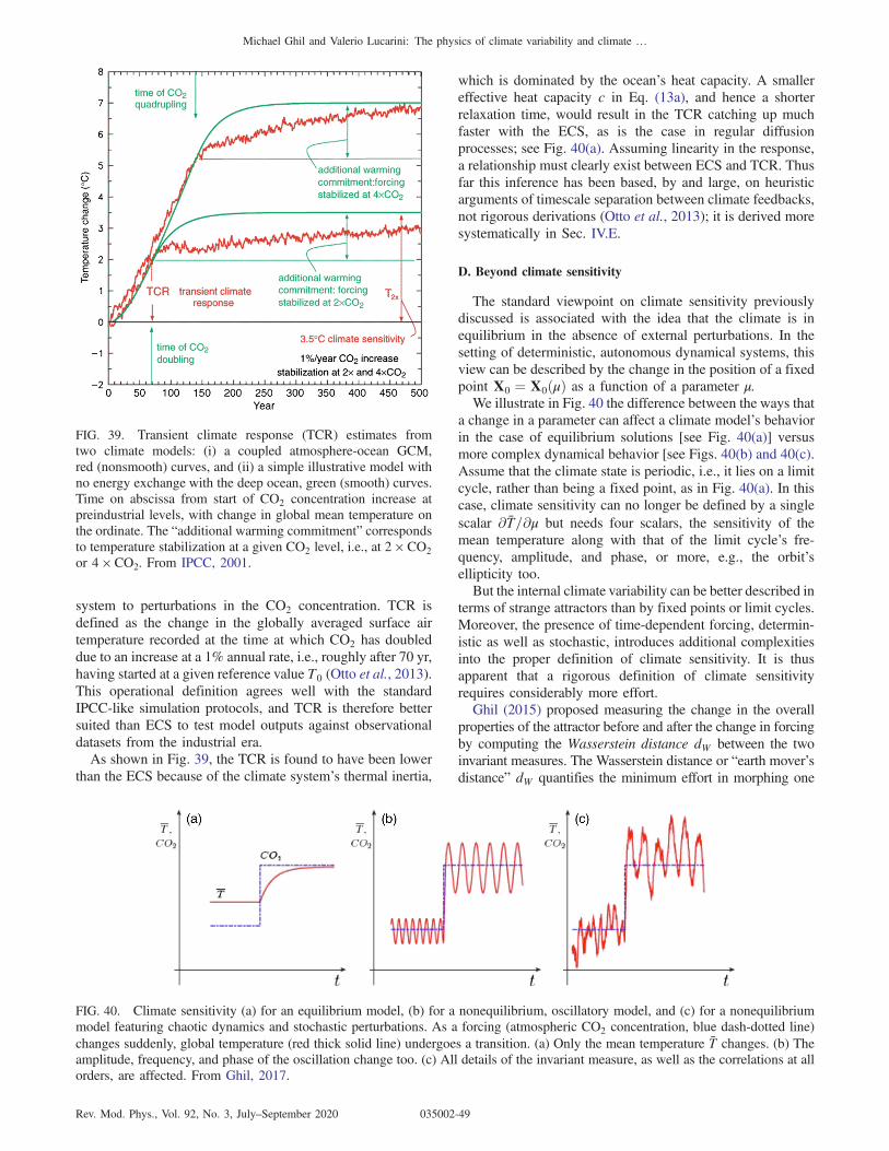
system to perturbations in the CO2 concentration. TCR isdefined as the change in the globally averaged surface airtemperature recorded at the time at which CO2 has doubleddue to an increase at a 1% annual rate, i.e., roughly after 70 yr,having started at a given reference value T0 (Otto et al., 2013).This operational definition agrees well with the standardIPCC-like simulation protocols, and TCR is therefore bettersuited than ECS to test model outputs against observationaldatasets from the industrial era.As shown in Fig. 39, the TCR is found to have been lower

than the ECS because of the climate system’s thermal inertia,

which is dominated by the ocean’s heat capacity. A smallereffective heat capacity c in Eq. (13a), and hence a shorterrelaxation time, would result in the TCR catching up muchfaster with the ECS, as is the case in regular diffusionprocesses; see Fig. 40(a). Assuming linearity in the response,a relationship must clearly exist between ECS and TCR. Thusfar this inference has been based, by and large, on heuristicarguments of timescale separation between climate feedbacks,not rigorous derivations (Otto et al., 2013); it is derived moresystematically in Sec. IV.E.

D. Beyond climate sensitivity

The standard viewpoint on climate sensitivity previouslydiscussed is associated with the idea that the climate is inequilibrium in the absence of external perturbations. In thesetting of deterministic, autonomous dynamical systems, thisview can be described by the change in the position of a fixedpoint X0 ¼ X0ðμÞ as a function of a parameter μ.We illustrate in Fig. 40 the difference between the ways that

a change in a parameter can affect a climate model’s behaviorin the case of equilibrium solutions [see Fig. 40(a)] versusmore complex dynamical behavior [see Figs. 40(b) and 40(c).Assume that the climate state is periodic, i.e., it lies on a limitcycle, rather than being a fixed point, as in Fig. 40(a). In thiscase, climate sensitivity can no longer be defined by a singlescalar ∂T=∂μ but needs four scalars, the sensitivity of themean temperature along with that of the limit cycle’s fre-quency, amplitude, and phase, or more, e.g., the orbit’sellipticity too.But the internal climate variability can be better described in

terms of strange attractors than by fixed points or limit cycles.Moreover, the presence of time-dependent forcing, determin-istic as well as stochastic, introduces additional complexitiesinto the proper definition of climate sensitivity. It is thusapparent that a rigorous definition of climate sensitivityrequires considerably more effort.Ghil (2015) proposed measuring the change in the overall

properties of the attractor before and after the change in forcingby computing the Wasserstein distance dW between the twoinvariant measures. The Wasserstein distance or “earth mover’sdistance” dW quantifies the minimum effort in morphing one

FIG. 39. Transient climate response (TCR) estimates fromtwo climate models: (i) a coupled atmosphere-ocean GCM,red (nonsmooth) curves, and (ii) a simple illustrative model withno energy exchange with the deep ocean, green (smooth) curves.Time on abscissa from start of CO2 concentration increase atpreindustrial levels, with change in global mean temperature onthe ordinate. The “additional warming commitment” correspondsto temperature stabilization at a given CO2 level, i.e., at 2 × CO2

or 4 × CO2. From IPCC, 2001.

FIG. 40. Climate sensitivity (a) for an equilibrium model, (b) for a nonequilibrium, oscillatory model, and (c) for a nonequilibriummodel featuring chaotic dynamics and stochastic perturbations. As a forcing (atmospheric CO2 concentration, blue dash-dotted line)changes suddenly, global temperature (red thick solid line) undergoes a transition. (a) Only the mean temperature T changes. (b) Theamplitude, frequency, and phase of the oscillation change too. (c) All details of the invariant measure, as well as the correlations at allorders, are affected. From Ghil, 2017.



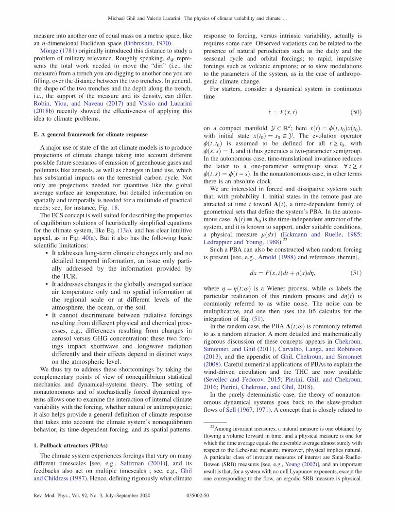
measure into another one of equal mass on a metric space, likean n-dimensional Euclidean space (Dobrushin, 1970).Monge (1781) originally introduced this distance to study a

problem of military relevance. Roughly speaking, dW repre-sents the total work needed to move the “dirt” (i.e., themeasure) from a trench you are digging to another one you arefilling, over the distance between the two trenches. In general,the shape of the two trenches and the depth along the trench,i.e., the support of the measure and its density, can differ.Robin, Yiou, and Naveau (2017) and Vissio and Lucarini(2018b) recently showed the effectiveness of applying thisidea to climate problems.

E. A general framework for climate response

A major use of state-of-the-art climate models is to produceprojections of climate change taking into account differentpossible future scenarios of emission of greenhouse gases andpollutants like aerosols, as well as changes in land use, whichhas substantial impacts on the terrestrial carbon cycle. Notonly are projections needed for quantities like the globalaverage surface air temperature, but detailed information onspatially and temporally is needed for a multitude of practicalneeds; see, for instance, Fig. 18.The ECS concept is well suited for describing the properties

of equilibrium solutions of heuristically simplified equationsfor the climate system, like Eq. (13a), and has clear intuitiveappeal, as in Fig. 40(a). But it also has the following basicscientific limitations:

• It addresses long-term climatic changes only and nodetailed temporal information, an issue only parti-ally addressed by the information provided bythe TCR.

• It addresses changes in the globally averaged surfaceair temperature only and no spatial information atthe regional scale or at different levels of theatmosphere, the ocean, or the soil.

• It cannot discriminate between radiative forcingsresulting from different physical and chemical proc-esses, e.g., differences resulting from changes inaerosol versus GHG concentration: these two forc-ings impact shortwave and longwave radiationdifferently and their effects depend in distinct wayson the atmospheric level.

We thus try to address these shortcomings by taking thecomplementary points of view of nonequilibrium statisticalmechanics and dynamical-systems theory. The setting ofnonautonomous and of stochastically forced dynamical sys-tems allows one to examine the interaction of internal climatevariability with the forcing, whether natural or anthropogenic;it also helps provide a general definition of climate responsethat takes into account the climate system’s nonequilibriumbehavior, its time-dependent forcing, and its spatial patterns.

1. Pullback attractors (PBAs)

The climate system experiences forcings that vary on manydifferent timescales [see, e.g., Saltzman (2001)], and itsfeedbacks also act on multiple timescales ; see, e.g., Ghiland Childress (1987). Hence, defining rigorously what climate

response to forcing, versus intrinsic variability, actually isrequires some care. Observed variations can be related to thepresence of natural periodicities such as the daily and theseasonal cycle and orbital forcings; to rapid, impulsiveforcings such as volcanic eruptions; or to slow modulationsto the parameters of the system, as in the case of anthropo-genic climate change.For starters, consider a dynamical system in continuous

time

_x ¼ Fðx; tÞ ð50Þ

on a compact manifold Y ⊂ Rd; here xðtÞ ¼ ϕðt; t0Þxðt0Þ,with initial state xðt0Þ ¼ x0 ∈ Y. The evolution operatorϕðt; t0Þ is assumed to be defined for all t ≥ t0, withϕðs; sÞ ¼ 1, and it thus generates a two-parameter semigroup.In the autonomous case, time-translational invariance reducesthe latter to a one-parameter semigroup since ∀ t ≥ sϕðt; sÞ ¼ ϕðt − sÞ. In the nonautonomous case, in other termsthere is an absolute clock.We are interested in forced and dissipative systems such

that, with probability 1, initial states in the remote past areattracted at time t toward AðtÞ, a time-dependent family ofgeometrical sets that define the system’s PBA. In the autono-mous case, AðtÞ≡A0 is the time-independent attractor of thesystem, and it is known to support, under suitable conditions,a physical measure μðdxÞ (Eckmann and Ruelle, 1985;Ledrappier and Young, 1988).22

Such a PBA can also be constructed when random forcingis present [see, e.g., Arnold (1988) and references therein],

dx ¼ Fðx; tÞdtþ gðxÞdη; ð51Þ

where η ¼ ηðt;ωÞ is a Wiener process, while ω labels theparticular realization of this random process and dηðtÞ iscommonly referred to as white noise. The noise can bemultiplicative, and one then uses the Itô calculus for theintegration of Eq. (51).In the random case, the PBA Aðt;ωÞ is commonly referred

to as a random attractor. A more detailed and mathematicallyrigorous discussion of these concepts appears in Chekroun,Simonnet, and Ghil (2011), Carvalho, Langa, and Robinson(2013), and the appendix of Ghil, Chekroun, and Simonnet(2008). Careful numerical applications of PBAs to explain thewind-driven circulation and the THC are now available(Sevellec and Fedorov, 2015; Pierini, Ghil, and Chekroun,2016; Pierini, Chekroun, and Ghil, 2018).In the purely deterministic case, the theory of nonauton-

omous dynamical systems goes back to the skew-productflows of Sell (1967, 1971). A concept that is closely related to

22Among invariant measures, a natural measure is one obtained byflowing a volume forward in time, and a physical measure is one forwhich the time average equals the ensemble average almost surely withrespect to the Lebesgue measure; moreover, physical implies natural.A particular class of invariant measures of interest are Sinai-Ruelle-Bowen (SRB) measures [see, e.g., Young (2002)], and an importantresult is that, for a system with no null Lyapunov exponents, except theone corresponding to the flow, an ergodic SRB measure is physical.



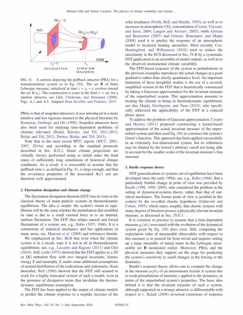
PBAs is that of snapshot attractors; it was introduced in a moreintuitive and less rigorous manner to the physical literature byRomeiras, Grebogi, and Ott (1990). Snapshot attractors havealso been used for studying time-dependent problems ofclimatic relevance (Bódai, Károlyi, and Tel, 2011,2013;Bódai and Tel, 2012; Drótos, Bódai, and Tel, 2015).Note that in the most recent IPCC reports (IPCC, 2001,

2007, 2014a) and according to the standard protocolsdescribed in Sec. II.D.2, future climate projections arevirtually always performed using as initial states the finalstates of sufficiently long simulations of historical climateconditions. As a result, it is reasonable to assume that thepullback time τ, as defined in Fig. 41, is large enough, and thatthe covariance properties of the associated AðtÞ sets aretherefore well approximated.

2. Fluctuation dissipation and climate change

The fluctuation-dissipation theorem (FDT) has its roots in theclassical theory of many-particle systems in thermodynamicequilibrium. The idea is simple: the system’s return to equi-librium will be the same whether the perturbation that modifiedits state is due to a small external force or to an internal,random fluctuation. The FDT thus relates natural and forcedfluctuations of a system; see, e,g., Kubo (1957, 1966). It is acornerstone of statistical mechanics and has applications inmany areas; see, Marconi et al. (2008) and references therein.We emphasized in Sec. III.B that even when the climate

system is in a steady state it is not at all in thermodynamicequilibrium; see, e.g., Lucarini and Ragone (2011) and Ghil(2019). Still, Leith (1975) showed that the FDTapplies to a 2Dor QG turbulent flow with two integral invariants, kineticenergy E and enstrophy Z, under some additional assumptionsof normal distribution of the realizations and stationarity. Soonthereafter, Bell (1980) showed that the FDT still seemed towork for a highly truncated version of such a model, even inthe presence of dissipative terms that invalidate the thermo-dynamic equilibrium assumption.The FDT has been applied to the output of climate models

to predict the climate response to a steplike increase of the

solar irradiance (North, Bell, and Hardin, 1993), as well as toincreases in atmospheric CO2 concentration (Cionni, Visconti,and Sassi, 2004; Langen and Alexeev, 2005), while Gritsunand Branstator (2007) and Gritsun, Branstator, and Majda(2008) used it to predict the response of an atmosphericmodel to localized heating anomalies. Most recently Cox,Huntingford, and Williamson (2018) tried to reduce theuncertainty in the ECS discussed in Sec. IV.B by a systematicFDTapplication to an ensemble of model outputs, as well as tothe observed instrumental climate variability.The FDT-based response of the system to perturbations in

the previous examples reproduces the actual changes at a goodqualitative rather than strictly quantitative level. An importantlimitation of these insightful studies is the use of a severelysimplified version of the FDT that is heuristically constructedby taking a Gaussian approximation for the invariant measureof the unperturbed system. This approximation amounts totreating the climate as being in thermodynamic equilibrium;see also Majda, Gershgorin, and Yuan (2010), who specifi-cally addressed the applicability of the FDT in a reducedphase space.To address the problem of Gaussian approximation, Cooper

and Haynes (2011) proposed constructing a kernel-basedapproximation of the actual invariant measure of the unper-turbed system and then used Eq. (56) to construct the system’sGreen’s function. This approach has been applied successfullyin an extremely low-dimensional system, but its robustnessmay be limited by the kernel’s arbitrary cutoff not being ableto account for the smaller scales of the invariant measure’s finestructure.

3. Ruelle response theory

FDT generalizations to systems out of equilibrium have beendeveloped since the early 1950s; see, e.g., Kubo (1966). But aparticularly fruitful change in point of view was provided byRuelle (1998, 1999, 2009), who considered the problem in thesetting of dynamical-systems theory, rather than that of stat-istical mechanics. The former point of view is justified in thiscontext by the so-called chaotic hypothesis (Gallavotti andCohen, 1995), which states, roughly, that chaotic systems withmany degrees of freedom possess a physically relevant invariantmeasure, as discussed in Sec. IV.E.1.It is common in practice to assume that a time-dependent

measure μtðdxÞ associated with the evolution of the dynamicalsystem given by Eq. (50) does exist. Still, computing theexpectation value of measurable observables with respect tothis measure is in general far from trivial and requires settingup a large ensemble of initial states in the Lebesgue meas-urable set B mentioned earlier. Moreover, PBAs and thephysical measures they support set the stage for predictingthe system’s sensitivity to small changes in the forcing or thedynamics.Ruelle’s response theory allows one to compute the change

in the measure μðdxÞ of an autonomous Axiom A system dueto weak perturbations of intensity ϵ applied to the dynamics, interms of the unperturbed system’s properties. The basic ideabehind it is that the invariant measure of such a system,although supported on a strange attractor, is differentiable withrespect to ϵ. Baladi (2008) reviewed extensions of response

FIG. 41. A cartoon depicting the pullback attractor (PBA) for anonautonomous system as in Eq. (50). The set B of finiteLebesgue measure, initialized at time t ¼ t0 − τ, evolves towardthe set Aðt0Þ. The construction is exact in the limit τ → ∞; for arandom attractor, see Ghil, Chekroun, and Simonnet (2008),Figs. A.1 and A.2. Adapted from Sevellec and Fedorov, 2015.



theory and provided a complementary approach to it, whileLucarini (2016) estimated its radius of convergence in ϵ.The establishment of a rigorous response theory is some-

what simpler in a sense if one considers stochastic instead ofstrictly deterministic processes (Hairer, 2010). Recently,Wormell (2019) clarified the link between the deterministicand stochastic perspectivesThe nonautonomous version of the Ruelle response theory

allows one to calculate the time-dependent measure μtðdxÞ onthe PBA by computing the time-dependent corrections to itwith respect to a reference state xðtÞ ¼ xðtÞ. This provides afairly general formulation for the climate system’s response toperturbations.Let us assume that we can write

_x ¼ Fðx; tÞ ¼ FðxÞ þ ϵXðx; tÞ; ð52Þ

where ∀ t ∈ R and ∀ x ∈ Y ⊂ Rd, jϵXðx; tÞj ≪ jFðxÞj.Hence, we can take FðxÞ as the background dynamics andϵXðx; tÞ as a perturbation. We treat here only the case ofdeterministic dynamics; see Lucarini (2012) for stochasticperturbations. As shown by Lucarini, Ragone, and Lunkeit(2017), we can restrict our analysis without loss of generalityto the separable case of Fðx; tÞ ¼ FðxÞ þ ϵXðxÞTðtÞ.To evaluate the expectation value hΨiϵðtÞ of a measurable

observable ΨðxÞ with respect to the measure μtðdxÞ of thesystem governed by Eq. (50), one writes

hΨiϵðtÞ ¼Z

ΨðxÞμtðdxÞ ¼ hΨi0 þX∞j¼1

ϵjhΨiðjÞ0 ðtÞ. ð53Þ

Here hΨi0 ¼RΨðxÞμðdxÞ is the expectation value of Ψ with

respect to the SRB invariant measure μðdxÞ of the autonomousdynamical system _x ¼ FðxÞ. We restrict ourselves here to thelinear correction term, which can be written as

hΨið1Þ0 ðtÞ ¼Z Z

∞

0

ΛSτ0ΨðxÞTðt − τÞdτμðdxÞ;

¼Z0

∞Gð1Þ

Ψ;XðτÞTðt − τÞdτ: ð54Þ

The Green’s function Gð1ÞΨ;XðτÞ in Eq. (54) is given by

Gð1ÞΨ;XðτÞ ¼

ZΘðτÞΛSτ0ΨðxÞμðdxÞ; ð55Þ

where Λð•Þ ¼ X ·∇ð•Þ and St0ð•Þ ¼ expðtF ·∇Þð•Þ is thesemigroup of unperturbed Koopman operators,23 ð·Þ denotesthe inner product in Y, and the Heaviside distribution ΘðτÞenforces causality. If the unperturbed invariant measure μðdxÞis smooth with respect to the standard Lebesgue measure, onehas μðdxÞ ¼ μðxÞdx, with μðxÞ the density, and the Green’sfunction can be written as follows:

Gð1ÞΨ;XðτÞ ¼ ΘðτÞ

Z−∇ · ½μðxÞX�

μðxÞ Sτ0ΨðxÞμðxÞdx

¼ ΘðτÞCðΦ; Sτ0ΨÞ. ð56Þ

Here Φ ¼ −f∇ · ½μðxÞX�g=μðxÞ and CðA; Sτ0BÞ is the τ-laggedcorrelation between the variables A and B, and the average ofΦ vanishes. Note that Eq. (56) is the appropriate generaliza-tion of the FDT for the nonautonomous, out-of-equilibriumsystem (52).Given any specific choice of the forcing’s time dependency

TðtÞ in Eqs. (52)–(54) and measuring the linear correction

term hΨið1Þ0 ðtÞ from a set of experiments, the same equationsallow one to derive the appropriate Green’s function.Therefore, using the output of a specific set of experimentsor of GCM simulations, we achieve predictive power for anytemporal pattern of the forcing XðxÞ.Consider now the Fourier transform of Eq. (54):

hΨið1Þ0 ðωÞ ¼ χð1ÞΨ;XðωÞTðωÞ; ð57Þ

where we introduce the susceptibility χð1ÞΨ;XðωÞ ¼ F ½Gð1ÞΨ;X�,

defined as the Fourier transform of the Green’s function

Gð1ÞΨ;XðtÞ. Under suitable integrability conditions, the fact that

the Green’s function GðtÞΨ;X is causal is equivalent to saying that

its susceptibility obeys the so-called Kramers-Kronig relations(Ruelle, 2009; Lucarini and Sarno, 2011); these provideintegral constraints that link the real and imaginary parts so

that χð1ÞΨ;XðωÞ ¼ iPð1=ωÞ⋆χð1ÞΨ;XðωÞ, where i ¼ ffiffiffiffiffiffi−1

p, ⋆ indi-

cates the convolution product, and P stands for integration byparts. Extensions to the case of higher-order susceptibilitiesare also available (Lucarini et al., 2005; Lucarini, 2008a,2009a; Lucarini and Colangeli, 2012).Instead of studying merely individual trajectories, one can

study the evolution of ensembles of trajectories to obtainprobabilistic estimates. The evolution of the measure ρ drivenby the dynamical system _x ¼ FðxÞ is described by the transferor Perron-Frobenius operator Lt

0 (Baladi, 2000; Villani, 2009;Chekroun et al., 2014), which is the adjoint of the Koopman orcomposition operator St0; it is defined as follows:

ZLt0ρðxÞΨðxÞdx ¼

ZρðxÞSt0ΨðxÞdx: ð58Þ

Assuming that no degenaracies are present, the generator ofthe semigroup fLt

0g is the so-called Liouville operator L and itsatisfies ∂tρ ¼ −∇ðρFÞ ¼ Lρ.Let fðσk; ρkÞ∶k ¼ 1;…;∞g be the eigenpairs of L. Then

the eigenvalues of Lt0 are given by fexpðσktÞg, with the same

eigenvectors fρkg. Correspondingly, the invariant measure μis the eigenvector having the null eigenvalue σ1 ¼ 0 for L or∀ t ≥ 0 unit eigenvalue of Lt

0. Note that ∀ k ≥ 2 ℜðσkÞ < 0,which implies exponential decay of correlations for all thesystem’s smooth observables, with an asymptotic rate that isgiven by the largest value of ℜðσkÞ, k ≥ 2. Moreover, thepresence of a small spectral gap between the unit eigenvalue ofLt0 and its other eigenvalues within the unit disk leads to a

23In discrete-time dynamics given by xkþ1 ¼ gðxkÞ, the Koopmanoperator is a linear operator acting on observables h∶Y → R viaUhðxÞ ¼ h(fðxÞ). In continuous-time dynamics like Eq. (50), thisoperator is replaced by a semigroup of operators, as in Eq. (55); seeBudivsić, Mohr, and Mezić (2012).



small radius of expansion for Ruelle’s perturbative approach(Chekroun et al., 2014; Lucarini, 2016).It turns out that if one neglects the essential part of the

spectrum, the susceptibility can be written as

χð1ÞΨ;XðωÞ ¼X∞k¼1

αkfΨ; Xgω − σk

; ð59Þ

where the factor αk evaluates how the response of the systemto the forcing X for the observable Ψ projects on theeigenvector fρkg. The constants πk ¼ iσk are usually referredto as Ruelle-Pollicott poles (Pollicott, 1985; Ruelle, 1986).Note that Eq. (59) implies that the Green’s function corre-sponding to the susceptibility can be written as a weightedsum of exponential functions if one neglects possibledegeneracies.24

4. Climate change prediction via Ruelle response theory

A somewhat different approach to constructing the climateresponse to forcings focuses on computing it directly fromEq. (55) without relying on the applicability of the FDT,which fails in certain cases of geophysical relevance; see, e.g.,Gritsun and Lucarini (2017). The difficulty in applying thisdirect approach lies in the fact that the formula containscontributions from both stable and unstable directions in thetangent space (Ruelle, 2009).Evaluating the contribution of the unstable directions is

especially hard; hence, Abramov and Majda (2007) proposeda blended approach that also uses the FDT. Using adjointmethods in the direct approach has yielded promising results(Wang, 2013). Faced with the so-called cold-start problem ofclimate simulations, Hasselmann et al. (1993) suggested aheuristic approach to computing a climate model’s Green’sfunction and applied it to study the relaxation to steady state ofa coupled GCM’s globally averaged surface temperatures.Lucarini and Sarno (2011), Ragone, Lucarini, and Lunkeit

(2016), and Lucarini, Ragone, and Lunkeit (2017) proposedevaluating the Green’s function using an experimental butrigorous approach suggested by standard optics laboratorypractice (Lucarini et al., 2005). The idea is to use a set ofcarefully selected probe experiments, typically, steplikeincreases of the parameter of interest, to construct theGreen’s function and then, exploiting Eq. (55), use thisoperator to predict the response of the system to a temporalpattern of interest for the forcing.Given a set of forced climate simulations and a background

unperturbed one, such an approach allows one to construct theGreen’s function’s response operators for as many observables

as desired, global as well as local in space. Such a tool kitallows one to treat a continuum of scenarios of temporalpatterns forcings, thus providing a general framework forimproving climate change projections given in the formshown in Fig. 18.The idea is to consider the set of equations describing

an unperturbed climate evolution in the form _x ¼ FðxÞ,with the vector field X ¼ XðxÞ in Eq. (52) as the 3Dradiative forcing associated with the increase of CO2 con-centration, and ϵTðtÞ its time modulation. By pluggingTðtÞ ¼ ϵΘðtÞ into Eq. (54), we have, for any climaticobservable Ψ,

ddt

hΨið1Þ0 ðtÞ ¼ ϵGð1ÞΨ;½CO2�ðtÞ: ð60Þ

We estimate hΨið1Þ0 ðtÞ by taking the system’s average ofresponse over an ensemble of initial states and use the

previous equation to derive our estimate of Gð1ÞΨ;½CO2�ðtÞ by

assuming linearity in the response.Note that these Green’s functions are specifically related to

changes in the atmospheric CO2 concentration, rather than to ageneric radiative forcing. Indeed, for each climatic variable,the response to changes in the solar irradiance, e.g., viamodulation of the parameter μ in Eq. (13), is different fromthe impact of changes in the CO2 concentration because thedetails of the radiative forcing are extremely different in thetwo cases. Thus, geoengineering proposals that aim to reducesolar irradiance by injecting sulphate aerosols into thestratosphere [see, e.g., Smith and Wagner (2018)] rely onflawed scientific reasoning (Lucarini, 2013; Bódai, Lucarini,and Lunkeit, 2020), are of dubious practical help (Proctoret al., 2018), and are hardly defensible from an ethicalperspective (Lawrence et al., 2018).Ragone, Lucarini, and Lunkeit (2016) derived, moreover, a

closed formula relating the TCR and the ECS. Indeed, withthe definition of TCRðτÞ given at the beginning of Sec. IV.C,one gets

ECS − TCRðτÞ¼ INRðτÞ

¼ ΔR2×CO2× P

Z∞

−∞χð1ÞTS;½CO2�ðω0Þ

×1þ ½sinðω0τ=2Þ=ðω0τ=2Þ� exp½−iω0τ=2�

2πiωdω0: ð61Þ

The difference between ECS and TCR is a weighted integralof the susceptibility, accounting for the contribution ofprocesses and feedbacks occurring at different timescales.

The integral in Eq. (61) yields χð1ÞTS;½CO2�ð0Þ if τ → 0 [i.e.,

TCRð0Þ ¼ 0], decreases with τ, and vanishes in the limitτ → ∞. INRðτÞ is a measure of the system’s inertia at thetimescale τ due to the overall contribution of the internalphysical processes and characteristic timescales of the relevantclimatic subsystems.Figure 42 illustrates a climate prediction obtained by

applying the previously mentioned response theory to the

24Note that Eq. (59) mirrors the quantum-mechanical expressionsfor the electric susceptibility of atoms or molecules. In the latter case,the summation involves all eigenstate pairs of the system’s unper-turbed Hamiltonian operator; in each term, the pole’s imaginary partcorresponds to the energy difference between the pair of consideredeigenstates, and the real part is the so-called linewidth of thetransition, whose inverse is the lifetime. Finally, the numerator isits so-called dipole strength (Cohen-Tannoudji, Dupont-Roc, andGrynberg, 2007).



open-source model PlaSim,25 an atmospheric GCM of inter-mediate complexity coupled with a mixed-layer ocean model(Fraedrich et al., 2005; Fraedrich, 2012). The figure showsgood agreement between (a) the ensemble average of 200simulations where the CO2 concentration is increased at therate of 1% until doubling (black curve), and then keptconstant, and (b) the prediction done by convolving theGreen’s function of Eq. (60) with the time pattern of theforcing (blue curve). Note that the temperature increasepredicted at year 70, when doubling of the CO2 is reached,gives as estimate the TCR ≃ 4.1 K (blue curve). The truevalue of the TCR ≃ 4.3 K is given by the black line. The TCRis indeed smaller than the ECS ≃ 4.8 K, which corresponds toa good approximation to the temperature increase predictedat year 200.The power of response theory lies in the fact that once the

Green’s function of interest has been computed one can predictthe future evolution of bespoke observables, defined as needed.Furthermore, Lucarini (2018) showed that it is possible to usecertain classes of observables as surrogate forcings of otherobservables, in the spirit of the linear feedback analysis ofEq. (44). Given the notoriously more difficult prediction ofprecipitation, Lucarini, Ragone, and Lunkeit (2017) found thatpredictions of changes in the globally averaged precipitationcan be as good as those of the temperature.Proceeding from global predictions to more localized ones,

Fig. 43 shows the outcome of predicting the change in thezonal averages of the surface temperature. It is clear thatresponse theory does a good job in reproducing the spatialpatterns of temperature change, except for an underestimateof the temperature change in the high latitudes on the scaleof few decades. Indeed, such a mishap is due the strongpolar amplification of the warming due to the ice-albedo

feedback, which can be qualitatively captured only by a linearapproach like the one used by Lucarini, Ragone, and Lunkeit(2017). A major limitation of the investigations by Ragone,Lucarini and Lunkeit (2016) and Lucarini, Ragone, andLunkeit (2017) was the use of a model unable to representexplicitly the dynamical processes of the global ocean. Morerecently, Lembo, Lucarini, and Ragone (2020) proved theeffectiveness of response theory in predicting the futureclimate response to CO2 on a vast range of temporal scales,from interannual to centennial, and for very diverse climaticvariables, including those representing the strength of theAtlantic Ocean’s meridional overturning circulation and ofthe ACC.

5. Slow correlation decay and sensitive parameter dependence

Equation (59) implies that resonant amplification occurs ifthe forcing acts as a frequency ω that is close to the imaginarypart of a subdominant Ruelle-Pollicott pole πk; k ≥ 2, that hasa small real part and corresponds therewith to a sharp spectralfeature, i.e., for some k ≥ 2,

jω − ℑðπkÞj ≪ ω; jℜðπkÞj ≪ ω; ð62Þbecause the system’s susceptibility is greatly enhanced at suchan ω. Conditions (62) are easily satisfied for a broadbandforcing and a system that has a small spectral gap. Conversely,as discussed after Eq. (58), the presence of a small spectral gapis associated with a slow decay of correlation for smooth

FIG. 42. Comparison between the climate model simulation(black line) and response theory prediction (blue line) for a TCRexperiment using PlaSim, a GCM of intermediate complexity.The CO2 concentration was ramped up by 1% per year to doubleits initial value. The upper and lower limit of the light-shadedbands are computed as 2 standard deviations of the ensembledistribution. From Lucarini, Ragone, and Lunkeit, 2017.

FIG. 43. Patterns of climate response for the zonal average ofthe surface temperature. (a) Prediction via response theory (redand black lines are not relevant in this context). (b) Differencebetween the ensemble average of the direct numerical simulationsand the predictions obtained using the response theory. FromLucarini, Ragone, and Lunkeit, 2017.

25See http://tiny.cc/zgk0bz.



http://tiny.cc/zgk0bz

http://tiny.cc/zgk0bz

observables. We now provide two examples that show howlinear response breaks down for forced systems possessingslow decay of correlations due to a small spectral gap in theunperturbed dynamics.The first example is due to Chekroun et al. (2014), who

investigated the response of the highly simplified ENSOmodel of Jin and Neelin (1993), to which Jin, Neelin, andGhil (1994) added periodic forcing that led to chaoticbehavior. Chekroun et al. focused on how the responsechanges when one varies the model parameter δ that controlsthe travel time of the equatorially trapped waves, which playan essential role in the ENSO mechanism. As shown inFig. 44, Chekroun et al. (2014) found that when the spectralgap is small the system exhibits rough dependence of itsproperties with respect to small modulations of the parameterssince Ruelle’s perturbative expansion breaks down even for anextremely small intensity of the forcing.The second example shows the importance of correlation

slowdown near saddle-node bifurcation points in the PlaSimmodel discussed in Sec. IV.E.4. This intermediate-complexitymodel is multistable: its bifurcation diagram with respect tothe solar insolation parameter μ is similar to Fig. 21; seeLucarini, Fraedrich, and Lunkeit (2010a) and Lucarini et al.(2013). PlaSim’s bifurcation diagram is reproduced inFig. 45(a), where the present climate S¼S0¼1360Wm−2

is denoted by a bullet and the bifurcation points associatedwith the transition from the warm to the snowball state W-SBand from the snowball to the warm state SB-W are indicatedby solid arrowheads. For a comparison with Fig. 21, note thatμ ¼ S=S0 there.Tantet et al. (2018) investigated PlaSim’s response to

changes in the solar irradiance for S < S0. They foundthat as the W-SB transition nears, the lag correlation for a

large-scale observable, namely the average equatorial near-surface air temperature, decays more and more slowly as aresult of a narrowing spectral gap. Indeed, near the saddle-node bifurcations, the response of the system to perturbationsis significantly amplified and, by definition, becomes singularexactly at the bifurcation point.More generally, Scheffer et al. (2009) proposed a set of

“early warning signals” (EWSs) that occur when a dynamicalsystem approaches a critical transition. Correlation slowdownis one of the main signals, and it is verified in the Tantet et al.(2018) case for the back-to-back saddle-node bifurcations thatmake up the backbone of the PlaSim model’s hysteresis cycle.Colon, Claessen, and Ghil (2015), though, found that in apredator-prey system—modeled either by a set of coupledODEs or by an agent-based model—more complex criticaltransitions can behave differently than in the simplest saddle-node case.Biggs, Carpenter, and Brock (2009) provided a broader

perspective on EWSs in the generic codimension-1

FIG. 44. Rough dependence (red dots) of the skewness of theequatorial ocean temperature’s distribution with respect tochanges in the parameter δ that controls the travel time ofequatorially trapped waves in a simplified ENSO model; seetext for details. Black points refer to nonchaotic windows wherethe parameter dependence is smooth; cyan points indicateparticularly sharp jumps in the parameter dependence. FromChekroun et al., 2014.

FIG. 45. Slowdown of correlations near a saddle-node bifurca-tion point in the PlaSim model. (a) The model’s bifurcationdiagram as a function of the value of the solar irradiance S. Thecritical transitions warm to snowball and snowball to warm aswell as the present-day conditions are indicated. From Lucarini,Fraedrich, and Lunkeit, 2010a. (b) Decay of correlation of theequatorial mean surface temperature for various values of thesolar irradiance S. The decay becomes considerably slower as Sapproaches the critical value of S ≃ 1265 Wm−2 . From Tantetet al., 2018.



bifurcations in multidimensional systems. The literature onEWSs, their successes, their failures, when they work andwhen they do not, is rich and beyond the scope of this review.These considerations naturally lead us to an inves-

tigation of the climate system’s global stability propertiesand its critical transitions, which are the subject of Sec. V.

V. CRITICAL TRANSITIONS AND EDGE STATES

In Sec. III, we introduced several types of bifurcations thatinvolve transitions between two or more regimes: saddle-nodebifurcations whose pairing can lead to coexistence of twostable steady states (fixed points), pitchfork bifurcations thatin the presence of a mirror symmetry can lead from one stablesymmetric steady state to the coexistence of two steady statesthat are mirror images of each other, Hopf bifurcations thatlead from a stable steady state to a stable periodic solution(limit cycle) and then again from the stable limit cycle to astable torus on which an infinity of quasiperiodic solutionslive, and nonlocal bifurcations associated with the existenceof homoclinic and heteroclinic orbits that lead to chaoticregimes.Successive-bifurcation scenarios (Eckmann, 1981; Ghil and

Childress, 1987; Dijkstra and Ghil, 2005; Dijkstra, 2013) thatinvolve several of these bifurcations and additional ones leadfrom solutions with high symmetry in space and time tosuccessively more complex and chaotic ones. We saw inSec. III that such bifurcation scenarios shed considerable lighton the phenomenology of large-scale atmospheric, oceanic,and coupled ocean-atmosphere flows. Finally, in Secs. III.Gand IV.E, we introduced stochastic effects into the nonlinearlydeterministic setting recalled previously and outlined the roleof PBAs and of the invariant measures they support in thetheory of nonautonomous and random dynamical systems(NDSs and RDSs).Recently the interest in bifurcations in the climate and

environmental sciences has signicantly increased due to theintroduction of the concept of tipping points from the socialsciences (Gladwell, 2000; Lenton et al., 2008). A tippingpoint sounds a lot more threatening than a bifurcation point,especially when dealing with a hurricane or dramatic andirreversible climate change.Beyond the linguistic effectiveness of the term, it does

also generalize the bifurcation concept in the context ofopen systems that are modeled mathematically by NDSs orRDSs. As we saw in Secs. III and II, the climate system.as well as its subsystems, namely, the atmosphere, ocean,biosphere, and cryosphere, are open and exchange time-dependent fluxes of mass, energy, and momentum with eachother and with outer space. Hence, it is quite appropriateto consider this generalization. Following Ashwin et al.

(2012), one distinguishes among three kinds of tippingpoints, as shown in Table II.The investigation of systems possessing multiple attractors,

which may include fixed points, limit cycles, strange attrac-tors, and PBAs or random attractors, is an active area ofresearch encompassing mathematics as well as the natural andsocioeconomic sciences. Feudel, Pisarchik, and Showalter(2018), for instance, provide a review that introduces a specialissue of the journal Chaos on the topic and sketch severalinteresting examples. More generally, Kuehn (2011) studiedtipping points and critical transitions in the NDS and RDScontext.This section is devoted to providing a general framework

for the study of multistability in the Earth system, to forcedtransitions between different regimes when multistability ispresent, and to the critical transitions taking place atclassical bifurcation and more general tipping points.Recall, for motivation, two cases of multistablility in theclimate system.First, Earth as a whole has boundary conditions that arise

from its space environment in the solar system that arecompatible with at least two competing stable regimes: today’srelatively ice-free and warm climate and a deep-freeze orsnowball climate; see Sec. III.A. Second, the ocean’s THC is,over a broad range of the parameters that control its heatand freshwater budget, bistable, with the current active statecoexisting with a greatly reduced or even reversed circulation;see Sec. III.C.To illustrate the main mathematical and physical aspects

of the problem, we choose at first the specific example ofcoexistence between the warmer Holocene-like state and themuch colder snowball state of Earth, as discussed inSecs. III.A and IV.E.5; see, in particular, Figs. 21 and 45(a).

A. Bistability for gradient flows and EBMs

The theory of SDEs and of RDSs provides a comprehensiveframework for deriving the probability of occurrence ofcoexisting regimes in multistable systems and for estimatingthe probability of stochastic-forcing-triggered transitionsbetween them. A good starting point is gradient flow in thepresence of additive white noise.The governing SDE in this case is

dx ¼ −∇xVðxÞdtþ ϵdW; ð63Þ

where x ∈ Rd, the potential V∶Rd → R is sufficientlysmooth, and dW is a vector of d independent increments ofBrownian motion, while ϵ determines the strength of thenoise. The Fokker-Planck equation associated with Eq. (63)describes the evolution of the PDF pϵðx; tÞ of an ensemble oftrajectories obeying the SDE.

TABLE II. Tipping points in open systems; see also Ashwin et al. (2012) and Fig. 46.

Type Cause Mechanism

B tipping Bifurcation-due tipping Slow change in a parameter leads to the system’s passage through a classical bifurcationN tipping Noise-induced tipping Random fluctuations lead to the system crossing an attractor basin boundaryR tipping Rate-induced tipping Because of rapid changes in the forcing, the system loses track of a slow change in its attractors



The stationary solution corresponding to the latter equa-tion’s invariant measure limt→∞ pϵðx; tÞ ¼ pϵðxÞ is given by alarge-deviation law (Varadhan, 1966)

pϵðxÞ ¼1

Zexp

�−2VðxÞϵ2

�; ð64Þ

where Z is a normalization constant. The local minima of thepotential V are the stable fixed points of the deterministicdynamics. One obtains them by setting ϵ ¼ 0 in the SDE (63),and they correspond to the local maxima of p. Thus, forinstance, the double-well potential of Fig. 20 corresponds to abimodal PDF.The mountain pass lemma [see, e.g., Bisgard (2015)] states

that the two minima of V that give rise to the two stable fixedpoints have to be separated by an unstable one of the saddletype, which is a maximum of V in one direction and aminimum in all other ones. Such a saddle looks like amountain pass on a topographic map (hence the name ofthe lemma). Ghil and Childress (1987) discussed in theirSec. 10.4 its application to 1D EBMs.In the limit of weak noise, trajectories starting near a local

minimum of V located at x ¼ x1 typically wait a long timebefore moving to the neighborhood of a different localminimum of V. The transitions are most likely to occurthrough the lowest energy saddle x ¼ xs that links the initialbasin of attraction to any other basin. Call the correspondinglocal minimum x ¼ x2.The optimal path linking x1 to xs minimizes the Freidlin and

Wentzell (1984) action and is called an instanton. In the weak-noise limit ϵ → 0, the persistence time inside the basin ofattraction of x ¼ x1 is

τϵ ∝ exp

�2½VðxsÞ − Vðx1Þ�

ϵ2

�; ð65Þ

which is referred to as the Kramers (1940) formula.Assume now, for simplicity, that we deal with a bistable

system, as in Fig. 20. If the potential V depends on a slowlyvarying control parameter ϕ, a B tipping would involve, for

instance, the number of local minima decreasing from 2 to 1,as a local minimum merges with a saddle point at ϕ ¼ ϕc.This merging is illustrated in Fig. 46 for a simple 1D case likethat of the 0D EBM governed by Eq. (13).26

When the system nears the tipping point, the persistencetime in the shallow, metastable minimum is reduced becauseΔV ≡ Vs − V1 → 0. Another flag anticipating the tippingpoint is the increase of the autocorrelation time τ in themetastable state, which is proportional to the inverse of thesecond derivative of the potential evaluated at the mini-mum τϵ ∝ 1=V 00

x1 .These two easily observable phenomena are the simplest

manifestation of the slowing-down process (Scheffer et al.,2009), which was discussed in Sec. IV.E.5 when describingthe findings of Tantet et al. (2018). As indicated in footnote 28there, the warning signals of the tipping-point approach havebeen studied mostly in the B-tipping case for saddle-nodebifurcations. Much remains to be done in this context for morecomplex situations that may involve N-tipping, R-tipping, orglobal bifurcations rather than local ones. For instance,Ditlevsen and Johnsen (2010) analyzed a high-resolutionice-core record and excluded the possibility of interpretingDansgaard-Oeschger events as B tipping by noting the lack ofthe two early warning signals mentioned previously. Theirresults leave us with the alternative of interpreting theassociated irregular oscillations [see, e.g., Boers, Ghil, andRousseau (2018)] either as the result of N tipping for anS-shaped back-to-back saddle-node bifurcation or asB tipping for a Hopf bifurcation; see Fig. 29 and its discussionin Sec. III.E.3 for similar ambiguities in interpreting changesin atmospheric LFV.Returning to the right-hand side of the 0D EBM of Eq. (13),

it can be written as minus the derivative of a potential VðTÞ;see Ghil (1976). The gain factor Λ given in Eq. (47), as well asthe ECS, is proportional to the inverse of the second derivativeof the potential V evaluated at the local minimum definingthe reference climate T0, ECS ∝ Λ ∝ 1=V 00

T0. Hence, near the

critical transition a small forcing in the right direction can leadthe system to jump to the other basin of attraction, even in theabsence of noise. Note, though, that near such a transition thelinear stability analysis performed in Eqs. (46) and (47) is nolonger valid, and an accurate quantitative analysis of climateresponse requires taking into account the essential nonlinear-ity in the problem; see the Zaliapin and Ghil (2010) commentson Roe and Baker (2007).Determining the saddle point that potentially connects, via

instantons, two local minima is not at all trivial when looking athigh- or even infinite-dimensional systems. Figure 47 reportsthe findings of Bódai et al. (2015) on the Ghil (1976) 1D EBM.Figure 47(a) shows the bifurcation diagram of the model, inwhich the control variable is the globally averaged surface airtemperature T, and the tuning parameter is the insolationparameter μ ¼ S=S0 introduced in Eq. (13b).Figure 47(b) shows the zonally averaged temperatures

of the 1D model’s steady states for the reference conditionsT ¼ TðxÞ at μ ¼ 1. The red and blue lines represent the two

FIG. 46. Schematic diagram of B tipping. As a control param-eter is slowly changed, the number of stable equilibria is reducedfrom 2 to 1. From Lenton et al., 2008.

26Note that the number of dimensions in phase space is 1, whilethat of the model in physical space is 0.



stable solutions, warm W and snowball SB, respectively,while the green line is the unstable solution lying between.Note that at each tipping point the unstable state comes incontact with a stable one and then both disappear, inaccordance with the scenario of basin boundary crisis (Ott,2002). In fact, the lack of stability of the steady-state solutiondescribed by the green line is apparent by observing that T inFig. 47(a) decreases with increasing solar radiation, asopposed to the W and SB states, which is clearly not physical(Ghil, 1976; North, Cahalan, and Coakley, 1981) and can beloosely interpreted as the result of a negative heat capacity; seeBódai et al. (2015).

B. Finding the edge states

In one phase space dimension, every first-order system_x ¼ fðx; μÞ is a gradient system since one can always writeVðx; μÞ ¼ −

Rfðξ; μÞdξ. This is not so in two or more

dimensions, and one might wonder whether it is possibleto compute unstable solutions for more general multistablesystems with no gradient property. Scott, Marotzke, and Stone(1999) presented an example of such an unstable stationary

solution in a simple box model of the THC featuringcompeting stable solutions and no gradient structure.Moreover, the actual computation of the unstable steady statein Fig. 3(a) of Ghil (1976) relied not on the system’s potentialV(TðxÞ) but on its 1D character in physical space and on ashooting method to solve the Sturm-Liouville equation thatresults when setting ∂Tðx; tÞ=∂t≡ 0 in the Ghil-Sellersmodel. Neither of these approaches (Ghil, 1976; Scott,Marotzke, and Stone, 1999) can easily be extended to moregeneral systems.In the remainder of this section, we discuss a more general

paradigm of multistability for determininistic systems and,subsequently, how this paradigm may be useful for studyingthe problem of noise-induced transitions between competingstates without the simplifying assumption of a gradient, asin Eq. (63).One can formally introduce general multistable systems as

follows. We consider a smooth autonomous continuous-timedynamical system acting on a smooth finite-dimensionalcompact manifold M, described by an ODE system of theform _x ¼ FðxÞ. The system is multistable if it possesses morethan one asymptotically stable state, defined by the attractorsfΩj∶j ¼ 1;…; Jg. The asymptotic state of an orbit is deter-mined by its initial state, and the phase space is partitionedbetween the basins of attraction fBjg of the attractors fΩjgand the boundaries f∂Bl∶l ¼ 1;…; Lg separating thesebasins.The basin boundaries can be strange geometrical objects

with a codimension smaller than 1. Orbits initialized on thebasin boundaries f∂Blg are attracted toward invariant saddlesfΠlk∶l ¼ 1;…; L; k ¼ 1;…; klg, where we allow for theexistence of kl separate saddles in the basin boundary ∂Bl;these saddles are often referred to as edge states; see Skufca,Yorke, and Eckhardt (2006) and Schneider, Eckhardt, andYorke (2007).27 For nongradient flows, the edge states, likethe asymptotic states, can feature chaotic dynamics (Grebogi,Ott, and Yorke, 1983; Robert et al., 2000; Ott, 2002; Vollmer,Schneider, and Eckhardt, 2009). Lucarini and Bódai (2017,2019, 2020) refer to the chaotic edge states as melancholia(M) states. Hence, we cannot expect to easily find edge statesand, a fortiori, M states for such general multistable systems.The edge tracking algorithm by Skufca, Yorke, and

Eckhardt (2006) and Schneider, Eckhardt, and Yorke(2007) allows one to do so by constructing a shadowingtrajectory that leads an orbit starting on the basin boundarytoward the corresponding edge state; see Fig. 48. Therein, oneuses a bisection method to control the instability associatedwith the trajectories’ divergence from the basin boundary.Bódai et al. (2015) first used edge tracking in a geophysicalcontext to reproduce the unstable solution of Ghil (1976) withthis more easily generalizable approach; compare to the greenline and circles in Fig. 47(b).Lucarini and Bódai (2017) computed M states for an

intermediate-complexity climate model with Oð105Þ degreesof freedom that couples PUMA, an atmospheric primitive

FIG. 47. Bistability for the Ghil-Sellers 1D EBM. (a) Simplifiedbifurcation diagram for the Ghil (1976) 1D EBM; compareFigs. 21 and 45. The red, blue, and green lines correspond to theglobally averaged surface air temperature for the warm, snowball,and melancholia states, respectively, as a function of the relativesolar irradiance μ; see also Arcoya, Diaz, and Tello (1998).(b) Meridional temperature profile for the warm state (red line),snowball state (blue line), and M state (green line) for this modelunder present-day conditions (μ ¼ 1), with the sine of latitude onthe x axis; compare to Ghil (1976), Fig. 3(a). The circles indicatethe M-state estimate obtained using the edge tracking method.Adapted from Bódai et al., 2015.

27Note that edge states refer to solutions separating long-livedturbulence and laminar flow, rather than the interface between trulyseparated attractor basins.



equation model (Frisius et al., 1998) with a modified versionof the 1D EBM of Ghil (1976) that acts as a surrogate oceanand contributes to meridional heat transport. Figure 49 showsthe bifurcation diagram of this climate model, where theW → SB tipping point is located near μ ¼ 0.98, while theSB → W tipping point is located near μ ¼ 1.06. Just as inthe 1D EBM of Fig. 47, the tipping points are associated withbasin boundary crises (Ott, 2002).Over a wide range of μ values, the edge state features

chaotic dynamics that arises from the atmospheric model’sbaroclinic instability; it leads to weather variability and to alimited predictability horizon. Since this instability is muchfaster than the climatic one due to the ice-albedo feedback, thebasin boundary is a fractal set with near-zero codimension, inagreement with results obtained in low-dimensional cases(Grebogi, Ott, and Yorke, 1983; Lai and Tel, 2011). In otherwords, the basin boundary has almost full Lebesgue measure.As a result, near the basin boundary there is virtually no

predictability on the asymptotic state of the system becauseinfinitesimally close initial states have a high probability ofbelonging to separate basins of attraction.

C. Invariant measures and noise-induced transitions

As mentioned previously, transitions across the basinboundaries of competing attractors are possible and quitelikely in the presence of stochastic perturbations. Noise-induced escape from an attractor has, in fact, long beenstudied in the natural sciences; see, e.g., Hanggi (1986), Kautz(1987), and Grassberger (1989).Let us generalize Eq. (63) as follows:

dx ¼ FðxÞdtþ ϵsðxÞdW. ð66Þ

Here x ∈ Rd, FðxÞdt is the drift term given by a vector flowfield that admits multiple steady states, as previously dis-cussed, and dW are the increments of a d-dimensionalBrownian motion. The volatility matrix sðxÞ ∈ Rd×d is suchthat sðxÞTsðxÞ is the covariance matrix of the noise. Finally,the parameter ϵ ≥ 0 controls the noise intensity.Recent extensions of the classical Freidlin and Wentzell

(1984) theory (Graham, Hamm, and Tel, 1991; Hamm, Tel,and Graham, 1994; Lai and Tel, 2011) yield results thatclosely mirror those summarized earlier in the case of gradientflows with additive noise [see Eqs. (64) and (65)], givensuitable assumptions on the drift term and the volatility; see,e.g., Lucarini and Bódai (2019, 2020). In the weak-noise limitgiven by ϵ → 0, the invariant measure of the system can bewritten as a large-deviation law. Formally, one must replaceVðxÞ with a general quasipotential ΦðxÞ, which depends in anontrivial way on FðxÞ and sðxÞ. Moreover, the constant Z inEq. (64) is replaced by a function ζðxÞ, which is relativelyunimportant because the behavior of the system dependsmostly on the properties of ΦðxÞ.Certain general properties of ΦðxÞ apply to all choices of

the noise law, and once a noise law is chosen one can derivehow the properties of the system change as a function of theparameter ϵ. In general, regardless of the noise law, ΦðxÞ haslocal minima supported on the attractors fΩj∶j ¼ 1;…; Jg ofthe deterministic dynamics. Correspondingly, the invariantmeasure has local maxima on the attractor. Moreover, ΦðxÞhas a constant value on the support of each edge state Πl andeach attractor Ωj.In the simplest case of J ¼ 2 attractors and L ¼ 1 edge state

in the basin boundary, in the weak-noise limit transitions awayfrom either attractor basin take place exponentially morelikely along the instanton connecting the correspondingattractor with the edge state Π1. As for the gradient flowsin Sec. V.A, instantons can be calculated as minimizers of asuitably defined action (Kautz, 1987; Grassberger, 1989;Kraut and Feudel, 2002; Beri et al., 2005).Consider now the case in which more than one edge state

separates a givenΩj from the other attractors fΩk∶k ≠ jg. Letus denote then by Πj the edge state for which the value ofΦ islowest. In this case, the most probable exit path connects Ωj

with Πj, while the other escape channels are basicallyswitched off in the weak-noise limit.

FIG. 48. Schematic diagram of the edge tracking algorithmproposed by Skufca, Yorke, and Eckhardt (2006) and Schneider,Eckhardt, and Yorke (2007) as applied to the 1D EBM of Fig. 47.From Bódai et al., 2015.

FIG. 49. Bifurcation diagram for the intermediate-complexityclimate model in Lucarini and Bódai (2017), drawn for thelong-term, globally averaged ocean temperatures ½hTSi�. Bist-ability is found for a large range of values of the controlparameter μ ¼ S=S0. The relevant solid lines are in red for thewarm W states, in blue for the snowball SB states, and in greenfor the melancholia M states, as in Fig. 47. From Lucarini andBódai, 2019.



Note that if the attractors and the edge states are morecomplex sets than isolated points, the instantons connectingthem are not unique because, in principle, any point of theattractor can be linked by an instanton to any point of the edgestate because the quasipotential is constant on Ωj and Πj.Indeed, the edge states are the gateways for the noise-inducedescapes from the deterministic basins of attraction, asillustrated in the bistable example with nongradient flowgiven later.Lucarini and Bódai (2019) introduced stochastic forcing

into the climate model studied by Lucarini and Bódai (2017)as a fluctuating factor of the form 1þ ϵdW=dt, where dW is aBrownian motion that modulates the solar insolationparameter μ. This forcing yields a multiplicative noise lawbecause the energy input into the system depends on theproduct of μ times the co-albedo (1 − α), where the albedoα ¼ αðTÞ depends explicitly on the surface air temperatureT ¼ Tðx; tÞ, which is a state variable of the model; comparewith Eq. (13b).In Fig. 50, we reproduce the estimate by Lucarini and Bódai

(2019) of a 2D projection of the invariant measure for μ ¼ 1

from a climate simulation of ≃6.0 × 104 yr with fluctuationsin the solar insolation of 1.5% on the scale of 100 yr. Thesimulation features 92 SB → W and W → SB transitions, andthe measure is projected onto the ð½TS�;ΔTSÞ plane; here ½TS�is the globally averaged surface air temperature and ΔTSmeasures the temperature difference between the surfacetemperature in the low- and high-latitude regions.The peaks of the PDFs are close to theW and SB attractors,

and the agreement improves even further when consideringthe two marginal PDFs (top left and bottom right insets). Both

the W → SB and SB → W instantons can be estimated: theirstarting and final points agree well with the attractors and theM state. The instantons follow a path of monotonic descentthat closely tracks the crests of the PDF, with the minimumoccurring at the M state.These features are all in excellent agreement with the

theoretical predictions for multistable systems with a gener-alized quasipotential.

D. Nearing critical transitions

The general framework outlined in Sec. V.C is also usefulfor studying the properties of such systems near a criticaltransition; see, e.g., Lucarini and Bódai (2019). In Fig. 49, it isclear that μ ¼ 0.98 is close to theW → SB tipping point. Onefinds that at low noise intensities, i.e., at a relative μfluctuation less than or equal to 1.4% on a centennial scale,it is extremely hard to escape from the SB state. This findinghappens to agree with snowball-state simulations that usedmore detailed models as well; see, e.g., Crowley, Hyde, andPeltier (2001), Pierrehumbert (2004), and Ghil (2019).Let us then focus on the escape from the W state. Lucarini

and Bódai (2019) estimated the expected value of thetransition time from theW to the SB state using 50 simulationsper noise strength value. These values grow exponentiallywith the inverse of the square of the parameter ϵ, as predictedby the theory; see Fig. 51(a). Note that the difference betweenthe quasipotential value Φ at the M state and at the W state isequal to half the slope of the straight line, which is inagreement with Eq. (65).Finally, the escape transition paths from the W state to the

M state are plotted in Fig. 51(b). In the weak-noise case ofrelative μ fluctuation smaller than 1% on a centennial scale,the highest densities of these paths lie quite close to theinstanton connecting theW attractor to theM state and followa path of decreasing probability.These encouraging results suggest that the underlying

methodology of edge tracking and instanton estimation couldbe applied to observational and reanalysis datasets. Asdiscussed in Sec. III.E.3, the episodic, or particle, approachto atmospheric LFV results in a Markov chain of regimesfRj∶j ¼ 1;…; Jg that involves preferential transition pathsfΘj;k∶j ¼ 1;…; J; k ¼ 1;…; Jg between them. Heretofore,these transition paths, as well as the regimes themselves, wereestimated by purely statistical methods; see Ghil et al. (2019)and Fig. 29(a). Deloncle et al. (2007) and Kondrashov et al.(2007) applied a random-forest algorithm (Breiman, 2001) tofind the best real-time predictors of the next regime in aMarkov chain, conditional upon the one currently occupied.The results were quite satisfying for the QG3 model byMarshall and Molteni (1993), and encouraging for an obser-vational dataset of 55 winters of Northern Hemisphere 700-hPa geopotential height anomalies; see Deloncle et al. (2007)and Kondrashov et al. (2007).

E. Chaos-to-chaos transition

Thus far we have seen that critical transitions associatedwith saddle-node bifurcations and mild generalizationsthereof are fairly well understood by now. We conclude this

FIG. 50. Invariant measure of the transitions between the twostable regimes of the stochastically perturbed climate model byLucarini and Bódai (2017) via the M state separating them forμ ¼ 1. (Main panel) Projection of this invariant measure on thereduced space ðTS; ½ΔTS�Þ. W attractor, red dot; SB attractor,blue dot; M state, green dot. Red and blue dashed lines plotthe W → SB and SB → W instantons, respectively. (Top leftinset) Marginal PDF with respect to ΔTS. (Bottom right inset)Marginal PDF with respect to ½TS�, (Center right inset)Probability along the two instantons. From Lucarini and Bódai,2019.



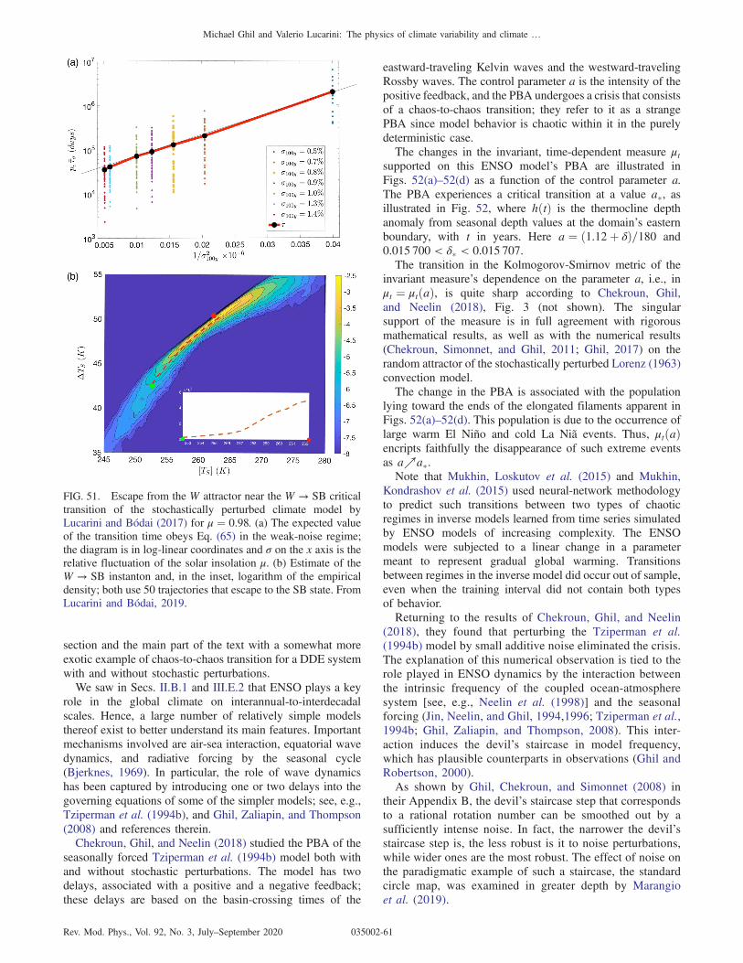
section and the main part of the text with a somewhat moreexotic example of chaos-to-chaos transition for a DDE systemwith and without stochastic perturbations.We saw in Secs. II.B.1 and III.E.2 that ENSO plays a key

role in the global climate on interannual-to-interdecadalscales. Hence, a large number of relatively simple modelsthereof exist to better understand its main features. Importantmechanisms involved are air-sea interaction, equatorial wavedynamics, and radiative forcing by the seasonal cycle(Bjerknes, 1969). In particular, the role of wave dynamicshas been captured by introducing one or two delays into thegoverning equations of some of the simpler models; see, e.g.,Tziperman et al. (1994b), and Ghil, Zaliapin, and Thompson(2008) and references therein.Chekroun, Ghil, and Neelin (2018) studied the PBA of the

seasonally forced Tziperman et al. (1994b) model both withand without stochastic perturbations. The model has twodelays, associated with a positive and a negative feedback;these delays are based on the basin-crossing times of the

eastward-traveling Kelvin waves and the westward-travelingRossby waves. The control parameter a is the intensity of thepositive feedback, and the PBA undergoes a crisis that consistsof a chaos-to-chaos transition; they refer to it as a strangePBA since model behavior is chaotic within it in the purelydeterministic case.The changes in the invariant, time-dependent measure μt

supported on this ENSO model’s PBA are illustrated inFigs. 52(a)–52(d) as a function of the control parameter a.The PBA experiences a critical transition at a value a�, asillustrated in Fig. 52, where hðtÞ is the thermocline depthanomaly from seasonal depth values at the domain’s easternboundary, with t in years. Here a ¼ ð1.12þ δÞ=180 and0.015 700 < δ� < 0.015 707.The transition in the Kolmogorov-Smirnov metric of the

invariant measure’s dependence on the parameter a, i.e., inμt ¼ μtðaÞ, is quite sharp according to Chekroun, Ghil,and Neelin (2018), Fig. 3 (not shown). The singularsupport of the measure is in full agreement with rigorousmathematical results, as well as with the numerical results(Chekroun, Simonnet, and Ghil, 2011; Ghil, 2017) on therandom attractor of the stochastically perturbed Lorenz (1963)convection model.The change in the PBA is associated with the population

lying toward the ends of the elongated filaments apparent inFigs. 52(a)–52(d). This population is due to the occurrence oflarge warm El Niño and cold La Niã events. Thus, μtðaÞencripts faithfully the disappearance of such extreme eventsas a↗a�.Note that Mukhin, Loskutov et al. (2015) and Mukhin,

Kondrashov et al. (2015) used neural-network methodologyto predict such transitions between two types of chaoticregimes in inverse models learned from time series simulatedby ENSO models of increasing complexity. The ENSOmodels were subjected to a linear change in a parametermeant to represent gradual global warming. Transitionsbetween regimes in the inverse model did occur out of sample,even when the training interval did not contain both typesof behavior.Returning to the results of Chekroun, Ghil, and Neelin

(2018), they found that perturbing the Tziperman et al.(1994b) model by small additive noise eliminated the crisis.The explanation of this numerical observation is tied to therole played in ENSO dynamics by the interaction betweenthe intrinsic frequency of the coupled ocean-atmospheresystem [see, e.g., Neelin et al. (1998)] and the seasonalforcing (Jin, Neelin, and Ghil, 1994,1996; Tziperman et al.,1994b; Ghil, Zaliapin, and Thompson, 2008). This inter-action induces the devil’s staircase in model frequency,which has plausible counterparts in observations (Ghil andRobertson, 2000).As shown by Ghil, Chekroun, and Simonnet (2008) in

their Appendix B, the devil’s staircase step that correspondsto a rational rotation number can be smoothed out by asufficiently intense noise. In fact, the narrower the devil’sstaircase step is, the less robust is it to noise perturbations,while wider ones are the most robust. The effect of noise onthe paradigmatic example of such a staircase, the standardcircle map, was examined in greater depth by Marangioet al. (2019).

FIG. 51. Escape from the W attractor near the W → SB criticaltransition of the stochastically perturbed climate model byLucarini and Bódai (2017) for μ ¼ 0.98. (a) The expected valueof the transition time obeys Eq. (65) in the weak-noise regime;the diagram is in log-linear coordinates and σ on the x axis is therelative fluctuation of the solar insolation μ. (b) Estimate of theW → SB instanton and, in the inset, logarithm of the empiricaldensity; both use 50 trajectories that escape to the SB state. FromLucarini and Bódai, 2019.



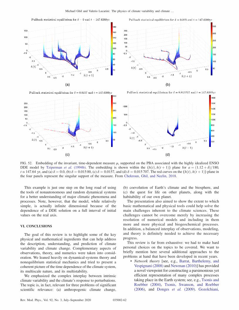
This example is just one step on the long road of usingthe tools of nonautonomous and random dynamical systemsfor a better understanding of major climatic phenomena andprocesses. Note, however, that the model, while relativelysimple, is actually infinite dimensional because of thedependence of a DDE solution on a full interval of initialvalues on the real axis.

VI. CONCLUSIONS

The goal of this review is to highlight some of the keyphysical and mathematical ingredients that can help addressthe description, understanding, and prediction of climatevariability and climate change. Complementary aspects ofobservations, theory, and numerics were taken into consid-eration. We leaned heavily on dynamical-systems theory andnonequilibrium statistical mechanics and tried to present acoherent picture of the time dependence of the climate system,its multiscale nature, and its multistability.We emphasized the complex interplay between intrinsic

climate variability and the climate’s response to perturbations.The topic is, in fact, relevant for three problems of significantscientific relevance: (a) anthropogenic climate change,

(b) coevolution of Earth’s climate and the biosphere, and(c) the quest for life on other planets, along with thehabitability of our own planet.The presentation also aimed to show the extent to which

basic mathematical and physical tools could help solve themain challenges inherent to the climate sciences. Thesechallenges cannot be overcome merely by increasing theresolution of numerical models and including in themmore and more physical and biogeochemical processes.In addition, a balanced interplay of observations, modeling,and theory is definitely needed to achieve the necessaryprogress.This review is far from exhaustive: we had to make hard

personal choices on the topics to be covered. We want tobriefly mention here several additional approaches to theproblems at hand that have been developed in recent years.

• Network theory [see, e.g., Barrat, Barthelemy, andVespignani (2008) and Newman (2010)] has provideda novel viewpoint for constructing a parsimonious yetefficient representation of many complex processestaking place in the Earth system; see, e.g., Tsonis andRoebber (2004), Tsonis, Swanson, and Roebber(2006), and Donges et al. (2009). Gozolchiani,

FIG. 52. Embedding of the invariant, time-dependent measure μt supported on the PBA associated with the highly idealized ENSODDE model by Tziperman et al. (1994b). The embedding is shown within the (hðtÞ; hðtþ 1Þ) plane for a ¼ ð1.12þ δÞ=180,t ≃ 147.64 yr, and (a) δ ¼ 0.0, (b) δ ¼ 0.015 00, (c) δ ¼ 0.0157, and (d) δ ¼ 0.015 707. The red curves on the (hðtÞ; hðtþ 1Þ) plane inthe four panels represent the singular support of the measure. From Chekroun, Ghil, and Neelin, 2018.



Havlin, and Yamasaki (2011) and Wang et al. (2013)provided examples of the use of networks forcapturing specific climatic processes, whileBoers et al. (2014) provided an example of applyingnetwork theory to climate prediction.

• Extreme value theory (EVT) [see, e.g., Embrechts,Kluppelberg, and Mikosch (1999) and Coles (2001)]has been used extensively in studying the statisticalproperties of rare hydrometeorological events, suchas the occurrence of intense rain or extreme temper-atures; see Katz, Parlange, and Naveau (2002),Ghil et al. (2011), and references therein. Yet thisclassical methodology has been almost entirelyneglected in IPCC reports dedicated to the studyof extremes; see IPCC (2012). Recently, though,rapid advances in EVT theory for general observ-ables of chaotic deterministic dynamical systems(Holland et al., 2012; Lucarini, Kuna et al., 2014;Lucarini et al., 2016) have led to the derivation ofindicators of weather regimes based on extremevalue statistics in the recurrence of atmosphericfields. In addition to the mere classification of suchregimes, as mentioned at the end of Sec. V.D, thisapproach allows one to infer higher or lowerinstability of these regimes, and hence their loweror higher predictability (Faranda, Messori, and Yiou,2017; Hochman et al., 2019).

• Large-deviation theory [see, e.g., Varadhan (1984)and Touchette (2009)] was first used in the contextof geophysical fluid dynamics for studying the self-organization and the multistability of turbulent flowsand, specifically, of jet structures (Bouchet andVenaille, 2012; Bouchet, Laurie, and Zaboronski,2014); see also Secs. V.A and V.C. More recentlyit has been applied successfully to the study ofweather and climate extremes. First, it has helpedformulate rare event algorithms able to nudge aclimate model toward representing preferentially theclass of extreme events of interest (Ragone, Wouters,and Bouchet, 2018). Second, it has provided a solidtheoretical and numerical basis for the study ofspatially extended or temporally persistent temper-ature extremes (Gálfi, Lucarini, and Wouters,2019). Large-deviation theory has also recently beenused to study multiscale and coupled atmosphere-ocean instabilities in a hierarchy of climate models(Vannitsem and Lucarini, 2016; De Cruz et al.,2018).

• Detection and attribution studies. In a complexsystem like the climate, inferring causal relationshipsamong events and phenomena is far from obvious.Nonetheless, doing so for well-defined weather andclimate events is essential for building simplifiedmodels and, at a practical level, for causal attributionof weather- and climate-related events. This is quiteimportant in the case of detection and attributionstudies of anthropogenic climate change, especially

when aiming to go beyond changes in mean climateproperties, such as globally averaged temperatures,and on to determining to what extent the occurrenceof an individual extreme event (e.g., of a hurricane oran extended drought) can be attributed to climatechange (Allen, 2003; Adam, 2011).

Methodologies based on the causal counterfactualtheory of Pearl (2009) are being increasingly recog-nized as a key instrument for providing a morerigorous basis for detection and attribution studies;see, e.g., Hannart, Pearl et al. (2016). They also seembetter suited for defining reliably the link betweenanthropogenic climate forcing and individual events(Hannart and Naveau, 2018). Combining these meth-ods with those of data assimilation, discussed inSec. II.A, appears to be well suited to refine thedistinction between the factual and counterfactualworld that separates causation from the lack thereof;see, e.g., Hannart, Carrassi et al. (2016).

• Beyond linear-response theory. As shown inSec. IV.E, linear-response theory can provide asystematic improvement upon the standard method-ology of forward integration of model ensembleswith perturbed initial states and parameters. While itdoes apply to systems out of thermodynamic equi-librium, it is still limited by its linearity to fairlysmall perturbations in parameters. In Sec. IV.D, wementioned that one can use the Wasserstein distanceto measure arbitrary changes between two invariantmeasures, whether supported on a time-independent,classical attractor or a time-dependent PBA. Onemight thus want to apply the PBA-based method-ologies herein directly to observational datasets or tothe simulations of IPCC-class models, either insteadof or in combination with previously tested statis-tical methods.

In Sec. V.E, we showed that the PBA of anintermediate but still infinite-dimensional ENSOmodel can undergo a chaos-to-chaos transition thatinvolves major changes in its invariant measure.Moreover, these changes could be connected to aphysically quite significant change in model behav-ior, namely, in the number and size of extremeevents, i.e., of the largest warm and cold events.Thus, exploring similarly interesting changes inmodel PBAs and in the time-dependent invariantmeasures supported by them appears to be a prom-ising road toward a deeper understanding of climatevariability and its interaction with both natural andanthropogenic forcing.

In this review, we have pointed out several open scientificproblems; see Ghil (2019) for a historical perspective. Animportant matter that was left practically untouched, asidefrom the brief discussion of ENSO and its prediction inSec. III.E.2, is the tropical atmosphere. Half of Earth’s surfacelies in the Tropics, between 30° N and 30° S, and much ofhumanity lives there. As one gets closer to the Equator, the



quasigeostrophic approximation collapses and moist proc-esses take on a much greater importance. Four of the classicalreferences are Palmer (1951), Riehl (1954), Krishnamurti,Stefanova, and Misra (1979), and Yanai (1975). The currentliterature is too plethoric to marshal here.We have also alluded, in Sec. I.B, to the increasing

importance of the issues discussed herein for the economicwell-being of our society and for the political decisionsneeded to mitigate climate change as well as adapt to it;see, for instance, IPCC (2014a, 2014b). A prudent way toaddress such decisions requires better estimates of theuncertainties involved; see, e.g., Barnett, Brock, andHansen (2020). Ghil (2020) provided an introduction torecent efforts at including the nonlinearities and stochasticitiesdiscussed herein in coupled climate-economy models foruncertainty quantification.More broadly, we alluded at the end of Sec. I to the lack of a

proper definition of climate and to the efforts to provide amathematically rigorous definition that would distinguish itfrom weather. We also mentioned in Sec. III.E.1 the distinctionmade by Von Neumann (1960) between the short-, medium-,and long-term prediction problem in the climate sciences.At an even higher level of abstraction, one might wish

to recall the parallel drawn by H. Poincare between thedeterministic unpredictability of weather and that of theposition of the planets on the ecliptic; see Poincare (1902),pp. 69 and 70. Harking back to these two giants of bothphysics and mathematics, we could say that (i) the astro-nomical ephemerides are the analog of weather and of itsshort-term prediction, (ii) the problem of climate correspondsto that of the long-term stability of the solar system, and(iii) the secular variations of the orbital configurations in theSolar System are the appropriate counterpart of the slowevolution of the climate system’s low-frequency modes ofvariability (Chown, 2004).Making these analogies stick at a level that might help

determine more reliably climate sensitivity to human activitiesis a worthwhile effort for the best mathematicians, physicists,and climate scientists.

LIST OF SYMBOLS AND ABBREVIATIONS

ACC Antarctic Circumpolar CurrentAR assessment reportAS Arakawa-Schubert (parametrization)CMIP Climate Model Intercomparison ProjectCNs complex networksDDE delay-differential equationDNS direct numerical simulationEBM energy balance modelECMWF European Centre for Mid-range Weather

ForecastsECS equilibrium climate sensitivityENSO El Niño–Southern OscillationEMS empirical model reductionEWS early warning signalFDT fluctuation-dissipation theoremGCM general circulation model

GCM global climate modelGFD geophysical fluid dynamicsGHGs greenhouse gasesGLE generalized Langevin equationIPCC Intergovernmental Panel on Climate

ChangeLFV low-frequency variabilityMJO Madden-Julian oscillationMOC meridional overturning circulationMZ Mori-ZwanzigNAO North Atlantic OscillationNCAR National Center for Atmospheric ResearchNCEP National Center for Environmental

PredictionNDS nonautonomous dynamical systemNWP numerical weather predictionNSEs Navier-Stokes equationsODE ordinary differential equationPBA pullback attractorPCMDI Program for Climate Model Diagnostics

and IntercomparisonPDE partial differential equationPNA Pacific North American (pattern)PSA Pacific South American (pattern)QG quasigeostrophic (flow, model)RDS random dynamical systemSDE stochastic differential equationSPM Summary for Policy MakersTCR transient climate responseTHC thermohaline circulationUNEP United Nations Environmental ProgrammeWCRP World Climate Research ProgrammeWMO World Meteorological Organization

ACKNOWLEDGMENTS

We benefited immensely from discussions with manycolleagues and friends in the last few years, but we especiallywant to thank T. Bódai, N. Boers, F. Bouchet, W. A. Brock,M. D. Chekroun, J. I. Díaz, H. A. Dijkstra, D. Faranda, A.Feigin, U. Feudel, K. Fraedrich, G. Froyland, G. Gallavotti, G.Gottwald, A. Gritsun, A. Groth, D. Holm, B. Hoskins, F.-F.Jin, D. Kondrashov, S. Kravtsov, J. Kurths, J. C. McWilliams,J. D. Neelin, S. Pierini, F. Ragone, D. Ruelle, A. Speranza, H.Swinney, O. Talagrand, A. Tantet, S. Vannitsem, J. Yorke, J.Wouters, and I. Zaliapin. Two anonymous reviewers providedconstructive comments. M. Cucchi suggested corrections inkey formulas when inspecting an earlier version of themanuscript. This review is TiPES contribution no. 19; theTiPES (Tipping Points in the Earth System) project hasreceived funding from the European Union’s Horizon 2020research and innovation program under Grant AgreementNo. 820970). This activity has been supported by the EITClimate-KIC. EIT Climate-KIC is supported by EIT, a body ofthe European Union. V L also acknowledges the financial



support provided by Horizon 2020 through the projectsCRESCENDO (Grant No. 641816) and Blue-Action (GrantNo. 727852), and by the Royal Society (Grant No. IEC R2170001).

REFERENCES

Abramov, R. V., and A. J. Majda, 2007, “Blended response algo-rithms for linear fluctuation-dissipation for complex nonlineardynamical systems,” Nonlinearity 20, 2793–2821.

Adam, D., 2011, “Climate change in court,” Nat. Clim. Change 1,127–130.

Allen, M., 2003, “Liability for climate change,” Nature (London)421, 891–892.

Andersen, K. K., et al. (North Greenland Ice Core Project Collabo-ration), 2004, “High-resolution record of Northern Hemisphereclimate extending into the last interglacial period,” Nature(London) 431, 147–151.

Andronov, A. A., and L. S. Pontryagin, 1937, “Structurally stablesystems,” Dokl. Akad. Nauk SSSR 14, 247–251.

Arakawa, A., and W. H. Schubert, 1974, “Interaction of a cumuluscloud ensemble with the large-scale environment. Part I,” J. Atmos.Sci. 31, 674–701.

Arcoya, D., J. I. Diaz, and L. Tello, 1998, “S-shaped bifurcationbranch in a quasilinear multivalued model arising in climatology,”J. Differ. Equations 150, 215–225.

Arnold, L., 1998, Random Dynamical Systems (Springer-Verlag,New York).

Arnold, Ludwig, 1988, Random Dynamical Systems (Springer,New York).

Arnold, V., 1983, Geometric Methods in the Theory of OrdinaryDifferential Equations (Springer, New York).

Arnold, V. I., 2003, Catastrophe Theory (Springer Nature, Berlin).Ashwin, P., S. Wieczorek, R. Vitolo, and P. Cox, 2012, “Tippingpoints in open systems: Bifurcation, noise-induced and rate-dependent examples in the climate system,” Phil. Trans. R. Soc.A 370, 1166–1184.

Baladi, V., 2000, Positive Transfer Operators and Decay ofCorrelations (World Scientific, Singapore).

Baladi, V., 2008, “Linear response despite critical points,”Nonlinearity 21, T81.

Balmaseda, M. A., et al., 2015, “The ocean reanalyses intercompar-ison project (ORA-IP),” J. Oper. Oceanogr. 8, s80–s97.

Barenblatt, G. L., 1987, Dimensional Analysis (Gordon and Breach,New York).

Barnes, E. A., and J. A. Screen, 2015, “The impact of Arctic warmingon the midlatitude jetstream: Can it? Has it? Will it?,”WIREs Clim.Change 6, 277–286.

Barnett, M., W. Brock, and L. P. Hansen, 2020, “Pricing uncertaintyinduced by climate change,” Rev. Financ. Stud. 33, 1024–1066.

Barnston, A. G., M. K. Tippett, M. L. Heureux, S. Li, and D. G.DeWitt, 2012, “Skill of real-time seasonal ENSOmodel predictionsduring 2002–2011—Is our capability improving?,” Bull. Am.Meteorol. Soc. 93, 631–651.

Barrat, A., M. Barthelemy, and A. Vespignani, 2008, DynamicalProcesses in Complex Networks (Cambridge University Press,Cambridge, England).

Batchelor, G., 1974, Introduction to Fluid Dynamics (CambridgeUniversity Press, Cambridge, England).

Beck, C., 1990, “Brownian motion from deterministic dynamics,”Physica (Amsterdam) 169A, 324–336.

Bell, T. L., 1980, “Climate sensitivity from fluctuation dissipation:Some simple model tests,” J. Atmos. Sci. 37, 1700–1707.

Bellenger, H., E. Guilyardi, J. Leloup, M. Lengaigne, and J. Vialard,2014, “Enso representation in climate models: From CMIP3 toCMIP5,” Clim. Dyn. 42, 1999–2018.

Bellman, R. E., and K. L. Cooke, 1963, Differential-DifferenceEquations (Rand Corporation, Santa Monica, CA).

Bengtsson, L., M. Ghil, and E. Kallen, 1981, Dynamic Meteorology:Data Assimilation Methods (Springer, New York).

Bensid, S., and J. I. Diaz, 2019, “On the exact number of monotonesolutions of a simplified Budyko climate model and their differentstability,” Discrete Contin. Dyn. Syst. B 24, 1033.

Benzi, R., P. Malguzzi, A. Speranza, and A. Sutera, 1986, “Thestatistical properties of general atmospheric circulation: Observa-tional evidence and a minimal theory of bimodality,” Q. J. R.Meteorol. Soc. 112, 661–674.

Benzi, R., and A. Speranza, 1989, “Statistical properties of low-frequency variability in the Northern Hemisphere,” J. Clim. 2,367–379.

Berger, A., and S. Siegmund, 2003, “On the gap between randomdynamical systems and continuous skew products,” J. Dyn. Differ.Equations 15, 237–279.

Beri, S., R. Mannella, D. G. Luchinsky, A. N. Silchenko, and P. V. E.McClintock, 2005, “Solution of the boundary value problemfor optimal escape in continuous stochastic systems and maps,”Phys. Rev. E 72, 036131.

Berloff, P., A. Hogg, and W. K. Dewar, 2007, “The turbulentoscillator: A mechanism of low-frequency variability of thewind-driven ocean gyres,” J. Phys. Oceanogr. 37, 2363–2386.

Berner, J., et al., 2017, “Stochastic parameterization: Toward a newview of weather and climate models,” Bull. Am. Meteorol. Soc. 98,565–588.

Bhattacharya, K., M. Ghil, and I. L. Vulis, 1982, “Internal variabilityof an energy-balance model with delayed albedo effects,” J. Atmos.Sci. 39, 1747–1773.

Biggs, R., S. R. Carpenter, and W. A. Brock, 2009, “Turning backfrom the brink: Detecting an impending regime shift in time to avertit,” Proc. Natl. Acad. Sci. U.S.A. 106, 826–831.

Bisgard, J., 2015, “Mountain passes and saddle points,” SIAM Rev.57, 275–292.

Bjerknes, J. P., 1969, “Atmospheric teleconnections from the equa-torial Pacific,” Mon. Weather Rev. 97, 163–172.

Bjerknes, V., 1904, “Das Problem der Wettervorhersage, betrachtetvom Standpunkte der Mechanik und der Physik,” Meteorol. Z. 21,1–7 [“The problem of weather prediction, considered from theviewpoints of mechanics and physics,” Meteorol. Z. 18, 663–667(2009)].

Bódai, T., G. Károlyi, and T. Tel, 2013, “Driving a conceptual modelclimate by different processes: Snapshot attractors and extremeevents,” Phys. Rev. E 87, 022822.

Bódai, T., Gy. Károlyi, and T. Tel, 2011, “A chaotically driven modelclimate: Extreme events and snapshot attractors,” NonlinearProcesses Geophys. 18, 573–580.

Bódai, T., V. Lucarini, and F. Lunkeit, 2020, “Can we use linearresponse theory to assess geoengineering strategies?,” Chaos 30,023124.

Bódai, T., V. Lucarini, F. Lunkeit, and R. Boschi, 2015,“Global instability in the Ghil-Sellers model,” Clim. Dyn. 44,3361–3381.

Bódai, T., and T. Tel, 2012, “Annual variability in a conceptualclimate model: Snapshot attractors, hysteresis in extreme events,and climate sensitivity,” Chaos 22, 023110.



https://doi.org/10.1088/0951-7715/20/12/004

https://doi.org/10.1038/nclimate1131


https://doi.org/10.1038/421891a

https://doi.org/10.1038/421891a

https://doi.org/10.1038/nature02805


https://doi.org/10.1175/1520-0469(1974)031%3C0674:IOACCE%3E2.0.CO;2

https://doi.org/10.1175/1520-0469(1974)031%3C0674:IOACCE%3E2.0.CO;2

https://doi.org/10.1006/jdeq.1998.3502

https://doi.org/10.1098/rsta.2011.0306


https://doi.org/10.1088/0951-7715/21/6/T01

https://doi.org/10.1080/1755876X.2015.1022329

https://doi.org/10.1002/wcc.337


https://doi.org/10.1093/rfs/hhz144

https://doi.org/10.1175/BAMS-D-11-00111.1


https://doi.org/10.1016/0378-4371(90)90173-P

https://doi.org/10.1175/1520-0469(1980)037%3C1700:CSFFDS%3E2.0.CO;2

https://doi.org/10.1007/s00382-013-1783-z

https://doi.org/10.3934/dcdsb.2019005

https://doi.org/10.1002/qj.49711247306

https://doi.org/10.1002/qj.49711247306

https://doi.org/10.1175/1520-0442(1989)002%3C0367:SPOLFV%3E2.0.CO;2

https://doi.org/10.1175/1520-0442(1989)002%3C0367:SPOLFV%3E2.0.CO;2

https://doi.org/10.1023/B:JODY.0000009736.39445.c4

https://doi.org/10.1023/B:JODY.0000009736.39445.c4

https://doi.org/10.1103/PhysRevE.72.036131

https://doi.org/10.1175/JPO3118.1



https://doi.org/10.1175/1520-0469(1982)039%3C1747:IVOAEB%3E2.0.CO;2

https://doi.org/10.1175/1520-0469(1982)039%3C1747:IVOAEB%3E2.0.CO;2

https://doi.org/10.1073/pnas.0811729106

https://doi.org/10.1137/140963510

https://doi.org/10.1137/140963510

https://doi.org/10.1175/1520-0493(1969)097%3C0163:ATFTEP%3E2.3.CO;2

https://doi.org/10.1127/0941-2948/2009/416

https://doi.org/10.1127/0941-2948/2009/416


https://doi.org/10.5194/npg-18-573-2011

https://doi.org/10.5194/npg-18-573-2011

https://doi.org/10.1063/1.5122255

https://doi.org/10.1063/1.5122255

https://doi.org/10.1007/s00382-014-2206-5

https://doi.org/10.1007/s00382-014-2206-5

https://doi.org/10.1063/1.3697984

Boers, N., B. Bookhagen, H. M. J. Barbosa, N. Marwan, J. Kurths,and J. A. Marengo, 2014, “Prediction of extreme floods in theEastern Central Andes based on a complex networks approach,”Nat. Commun. 5, 5199.

Boers, N., M. Ghil, and D.-D. Rousseau, 2018, “Ocean circulation,ice shelf, and sea ice interactions explain Dansgaard-Oeschgercycles,” Proc. Natl. Acad. Sci. U.S.A. 115, E11005–E11014.

Boiseau, M., M. Ghil, and A. Juillet-Leclerc, 1999, “Trends andinterdecadal variability from South-Central Pacific coral records,”Geophys. Res. Lett. 26, 2881–2884.

Bond, G., W. Showers, M. Cheseby, R. Lotti, P. Almasi, P.deMenocal, P. Priori, H. Cullen, I. Hajdas, and G. Bonani,1997, “A pervasive millennial-scale cycle in the North AtlanticHolocene and glacial climates,” Science 278, 1257–1265.

Bony, S., et al., 2015, “Clouds, circulation and climate sensitivity,”Nat. Geosci. 8, 261–268.

Boos, W. R., and J. V. Hurley, 2013, “Thermodynamic bias in themultimodel mean boreal summer monsoon,” J. Clim. 26.

Bouchet, F., J. Laurie, and O. Zaboronski, 2014, “Langevin dynamics,large deviations and instantons for the quasi-geostrophic model andtwo-dimensional Euler equations,” J. Stat. Phys. 156, 1066–1092.

Bouchet, F., and J. Sommeria, 2002, “Emergence of intense jets andJupiter’s Great Red Spot as maximum-entropy structures,” J. FluidMech. 464, 165–207.

Bouchet, F., and A. Venaille, 2012, “Statistical mechanics of two-dimensional and geophysical flows,” Phys. Rep. 515, 227–295.

Branstator, G., 1987, “A striking example of the atmosphere’s leadingtraveling pattern,” J. Atmos. Sci. 44, 2310–2323.

Breiman, L., 2001, “Random forests,” Mach. Learn. 45, 5–32.Broecker, W. S., 1991, “The great ocean conveyor,” Oceanography 4,79–89.

Bryan, F. O., 1986, “High-latitude salinity effects and interhemi-spheric thermohaline circulations,”Nature (London) 323, 301–304.

Budivsić, M., R. Mohr, and I. Mezić, 2012, “Applied Koopmanism,”Chaos 22, 047510.

Budyko, M. I., 1969, “The effect of solar radiation variations on theclimate of the Earth,” Tellus 21, 611–619.

Cane, M. A., and S. E. Zebiak, 1985, “A theory for El Nińo and theSouthern Oscillation,” Science 228, 1085–1087.

Caraballo, T., and X. Han, 2017, Applied Nonautonomous andRandom Dynamical Systems: Applied Dynamical Systems(Springer Science+Business Media, New York).

Carrassi, A., M. Bocquet, L. Bertino, and G. Evensen, 2018, “Dataassimilation in the geosciences: An overview of methods, issues,and perspectives,” WIREs Clim. Change 9, e535.

Carton, J. A., and B. S. Giese, 2008, “A reanalysis of ocean climateusing Simple Ocean Data Assimilation (SODA),” Mon. WeatherRev. 136, 2999–3017.

Carvalho, A. N., J. Langa, and J. C. Robinson, 2013, “The pullbackattractor,” in Attractors for Infinite-Dimensional Non-autonomousDynamical Systems, Applied Mathematical Sciences Vol. 182(Springer New York), pp. 3–22.

Cessi, P., 2019, “The global overturning circulation,” Annu. Rev.Mar. Sci. 11, 249–270.

Cessi, P., and G. R. Ierley, 1995, “Symmetry-breaking multipleequilibria in quasi-geostrophic, wind-driven flows,” J. Phys.Oceanogr. 25, 1196–1205.

Cessi, P., and W. R. Young, 1992, “Multiple equilibria in two-dimensional thermohaline circulation,” J. Fluid Mech. 241,291–309.

Chang, C. P., M. Ghil, M. Latif, and J. M. Wallace, Eds., 2015,Climate Change: Multidecadal and Beyond (World Scientific,Singapore).

Chang, K-Il, M. Ghil, K. Ide, and C-C. A. Lai, 2001, “Transition toaperiodic variability in a wind-driven double-gyre circulationmodel,” J. Phys. Oceanogr. 31, 1260–1286.

Charney, J. G., 1947, “The dynamics of long waves in a baroclinicwesterly current,” J. Meteorol. 4, 136–162.

Charney, J. G., 1971, “Geostrophic turbulence,” J. Atmos. Sci. 28,1087–1095.

Charney, J. G., A. Arakawa, D. J. Baker, B. Bolin, R. E. Dickinson,R. M. Goody, C. E. Leith, H. M. Stommel, and C. I. Wunsch, 1979,Carbon Dioxide and Climate: A Scientific Assessment (NationalAcademy of Sciences, Washington, DC).

Charney, J. G., and J. G. DeVore, 1979, “Multiple flow equilibria inthe atmosphere and blocking,” J. Atmos. Sci. 36, 1205–1216.

Charney, J. G., R. Fjørtoft, and J. von Neumann, 1950, “Numericalintegration of the barotropic vorticity equation,” Tellus 2,237–254.

Charney, J. G., M. Halem, and R. Jastrow, 1969, “Use of incompletehistorical data to infer the present state of the atmosphere,”J. Atmos. Sci. 26, 1160–1163.

Charney, J. G., J. Shukla, and K. C. Mo, 1981, “Comparison of abarotropic blocking theory with observation,” J. Atmos. Sci. 38,762–779.

Chavanis, P. H., and J. Sommeria, 1996, “Classification of self-organized vortices in two-dimensional turbulence: The case of abounded domain,” J. Fluid Mech. 314, 267–297.

Chekroun, M. D., M. Ghil, and J. D. Neelin, 2018, “Pullback attractorcrisis in a delay differential ENSO model,” in Advances in Non-linear Geosciences, edited by A. Tsonis (Springer, New York),pp. 1–33.

Chekroun, M. D., J. D. Neelin, D. Kondrashov, J. C. McWilliams,and M. Ghil, 2014, “Rough parameter dependence in climatemodels and the role of Ruelle-Pollicott resonances,” Proc. Natl.Acad. Sci. U.S.A. 111, 1684–1690.

Chekroun, M. D., E. Simonnet, and M. Ghil, 2011, “Stochasticclimate dynamics: Random attractors and time-dependent invariantmeasures,” Physica (Amsterdam) 240D, 1685–1700.

Chen, F., and M. Ghil, 1996, “Interdecadal variability in ahybrid coupled ocean-atmosphere model,” J. Phys. Oceanogr.26, 1561–1578.

Cheng, X., and J. M. Wallace, 1993, “Cluster analysis of the NorthernHemisphere wintertime 500 pHa heigh field: Spatial patterns,”J. Atmos. Sci. 50, 2674–2696.

Chorin, A., and P. Stinis, 2007, “Problem reduction, renormalization,and memory,” Commun. Appl. Math. Comput. Sci. 1, 1–27.

Chorin, A. J., O. H. Hald, and R. Kupferman, 2002, “Optimalprediction with memory,” Physica (Amsterdam) 166D, 239–257.

Chown, M., 2004, “Chaotic heavens,” New Sci. 181, 32–35.Cionni, I., G. Visconti, and F. Sassi, 2004, “Fluctuation dissipationtheorem in a general circulation model,” Geophys. Res. Lett. 31,https://doi.org/10.1029/2004GL019739.

Cohen-Tannoudji, C., J. Dupont-Roc, and G. Grynberg, 2007,Photons and Atoms: Introduction to Quantum Electrodynamics(Wiley, New York).

Coles, S., 2001, An Introduction to Statistical Modeling of ExtremeValues (Springer Science+Business Media, New York).

Colon, C., D. Claessen, and M. Ghil, 2015, “Bifurcation analysis ofan agent-based model for predator-prey interactions,” Ecol. Modell.317, 93–106.

Compo, G. P., et al., 2011, “The twentieth century reanalysisproject,” Q. J. R. Meteorol. Soc. 137, 1–28.

Cooper, F. C., and P. H. Haynes, 2011, “Climate sensitivity via anonparametric fluctuation-dissipation theorem,” J. Atmos. Sci. 68,937–953.



https://doi.org/10.1038/ncomms6199


https://doi.org/10.1029/1999GL900595

https://doi.org/10.1126/science.278.5341.1257

https://doi.org/10.1038/ngeo2398

https://doi.org/10.1175/JCLI-D-12-00493.1

https://doi.org/10.1007/s10955-014-1052-5

https://doi.org/10.1017/S0022112002008789

https://doi.org/10.1017/S0022112002008789

https://doi.org/10.1016/j.physrep.2012.02.001

https://doi.org/10.1175/1520-0469(1987)044%3C2310:ASEOTA%3E2.0.CO;2

https://doi.org/10.1023/A:1010933404324

https://doi.org/10.5670/oceanog.1991.07


https://doi.org/10.1038/323301a0

https://doi.org/10.1063/1.4772195

https://doi.org/10.3402/tellusa.v21i5.10109



https://doi.org/10.1175/2007MWR1978.1

https://doi.org/10.1175/2007MWR1978.1

https://doi.org/10.1146/annurev-marine-010318-095241

https://doi.org/10.1146/annurev-marine-010318-095241

https://doi.org/10.1175/1520-0485(1995)025%3C1196:SBMEIQ%3E2.0.CO;2

https://doi.org/10.1175/1520-0485(1995)025%3C1196:SBMEIQ%3E2.0.CO;2

https://doi.org/10.1017/S0022112092002040

https://doi.org/10.1017/S0022112092002040

https://doi.org/10.1175/1520-0485(2001)031%3C1260:TTAVIA%3E2.0.CO;2

https://doi.org/10.1175/1520-0469(1947)004%3C0136:TDOLWI%3E2.0.CO;2

https://doi.org/10.1175/1520-0469(1971)028%3C1087:GT%3E2.0.CO;2

https://doi.org/10.1175/1520-0469(1971)028%3C1087:GT%3E2.0.CO;2

https://doi.org/10.1175/1520-0469(1979)036%3C1205:MFEITA%3E2.0.CO;2



https://doi.org/10.1175/1520-0469(1969)026%3C1160:UOIHDT%3E2.0.CO;2

https://doi.org/10.1175/1520-0469(1981)038%3C0762:COABBT%3E2.0.CO;2

https://doi.org/10.1175/1520-0469(1981)038%3C0762:COABBT%3E2.0.CO;2

https://doi.org/10.1017/S0022112096000316



https://doi.org/10.1016/j.physd.2011.06.005

https://doi.org/10.1175/1520-0485(1996)026%3C1561:IVIAHC%3E2.0.CO;2

https://doi.org/10.1175/1520-0485(1996)026%3C1561:IVIAHC%3E2.0.CO;2

https://doi.org/10.1175/1520-0469(1993)050%3C2674:CAOTNH%3E2.0.CO;2

https://doi.org/10.2140/camcos.2006.1.1

https://doi.org/10.1016/S0167-2789(02)00446-3

https://doi.org/10.1029/2004GL019739

https://doi.org/10.1016/j.ecolmodel.2015.09.004

https://doi.org/10.1016/j.ecolmodel.2015.09.004

https://doi.org/10.1002/qj.776

https://doi.org/10.1175/2010JAS3633.1

https://doi.org/10.1175/2010JAS3633.1

Cox, P. M., C. Huntingford, and M. S. Williamson, 2018, “Emergentconstraint on equilibrium climate sensitivity from global temper-ature variability,” Nature (London) 553, 319–322.

Cronin, T. N., 2010, Paleoclimates: Understanding Climate ChangePast and Present (Columbia University Press, New York).

Crowley, T. J., W. T. Hyde, and W. R. Peltier, 2001, “CO2 levelsrequired for deglaciation of a ‘near-snowball’ Earth,” Geophys.Res. Lett. 28, 283–286.

Cushman-Roisin, B., and J.-M. Beckers, 2011, Introduction toGeophysical Fluid Dynamics: Physical and Numerical Aspects(Academic Press, New York), p. 875.

Cvitanović, Predrag, 1988, “Invariant measurement of strange sets interms of cycles,” Phys. Rev. Lett. 61, 2729–2732.

Cvitanovíc, P., and B. Eckhardt, 1991, “Periodic orbit expansions forclassical smooth flows,” J. Phys. A 24, L237.

Da Costa, E. D., and A. C. Colin de Verdiere, 2002, “The 7.7 yearNorth Atlantic Oscillation,” Q. J. R. Meteorol. Soc. 128,797–817.

Dansgaard, W., et al., 1993, “Evidence for general instability of pastclimate from a 250-kyr ice-core record,” Nature (London) 364,218–220.

Davini, P., and F. D’Andrea, 2016, “Northern Hemisphere atmos-pheric blocking representation in global climate models: Twentyyears of improvements?,” J. Clim. 29, 8823–8840.

De Cruz, L., S. Schubert, J. Demaeyer, V. Lucarini, and S. Vannitsem,2018, “Exploring the Lyapunov instability properties of high-dimensional atmospheric and climate models,”Nonlinear ProcessesGeophys. 25, 387–412.

Dee, D. P., et al., 2011, “The ERA-Interim reanalysis: Configurationand performance of the data assimilation system,” Q. J. R.Meteorol. Soc. 137, 553–597.

de Groot, S. R., and P. Mazur, 1984, Non-Equilibrium Thermo-dynamics (Dover, New York).

Dell’Aquila, A., V. Lucarini, P. M. Ruti, and S. Calmanti, 2005,“Hayashi spectra of the Northern Hemisphere mid-latitude atmos-pheric variability in the NCEP and ERA-40 reanalyses,”Clim. Dyn.25, 639–652.

Dell’Aquila, A., P. M. Ruti, S. Calmanti, and V. Lucarini, 2007,“Southern Hemisphere midlatitude atmospheric variability of theNCEP-NCAR and ECMWF reanalyses,” J. Geophys. Res. 112,D08106.

Deloncle, A., R. Berk, F. D’Andrea, and M. Ghil, 2007, “Weatherregime prediction using statistical learning,” J. Atmos. Sci. 64,1619–1635.

Delworth, T., S. Manabe, and R. J. Stouffer, 1993, “Interdecadalvariations of the thermohaline circulation in a coupled ocean-atmosphere model,” J. Clim. 6, 1993–2011.

Delworth, T. L., and M. E. Mann, 2000, “Observed and simulatedmultidecadal variability in the Northern Hemisphere,” Clim. Dyn.16, 661–676.

Demaeyer, J., and S. Vannitsem, 2017, “Stochastic parametrization ofsubgrid-scale processes in coupled ocean-atmosphere systems:Benefits and limitations of response theory,” Q. J. R. Meteorol.Soc. 143, 881–896.

Dickey, J. O., M. Ghil, and S. L. Marcus, 1991, “Extratropical aspectsof the 40–50 day oscillation in length-of-day and atmosphericangular momentum,” J. Geophys. Res. 96, 22643–22658.

Dijkstra, H. A., 2005, Nonlinear Physical Oceanography: A Dynami-cal Systems Approach to the Large Scale Ocean Circulation and ElNiño., 2nd ed. (Springer Science+Business Media., Berlin).

Dijkstra, H. A., 2007, “Characterization of the multiple equilibriaregime in a global ocean model,” Tellus A 59, 695–705.

Dijkstra, H. A., 2013, Nonlinear Climate Dynamics (CambridgeUniversity Press, Cambridge, England).

Dijkstra, H. A., and G. Burgers, 2002, “Fluid mechanics of El Niñovariability,” Annu. Rev. Fluid Mech. 34, 531–558.

Dijkstra, H. A., and M. Ghil, 2005, “Low-frequency variability of thelarge-scale ocean circulation: A dynamical systems approach,” Rev.Geophys. 43, RG3002.

Dijkstra, H. A., and C. A. Katsman, 1997, “Temporal variability ofthe wind-driven quasi-geostrophic double gyre ocean circulation:Basic bifurcation diagrams,” Geophys. Astrophys. Fluid Dyn. 85,195–232.

Ditlevsen, P. D., and S. J. Johnsen, 2010, “Tipping points: Earlywarning and wishful thinking,” Geophys. Res. Lett. 37.

Doblas-Reyes, Francisco J., Javier Garcia-Serrano, Fabian Lienert,Aida Pinto Biescas, and Luis R. L. Rodrigues, 2013, “Seasonalclimate predictability and forecasting: status and prospects,”WIREs Clim. Change 4, 245–268.

Dobrushin, R., 1970, “Prescribing a system of random variables byconditional distributions,” Theory Probab. Appl. 15, 458–486.

Donges, J. F., Y. Zou, N. Marwan, and J. Kurths, 2009, “Complexnetworks in climate dynamics,” Eur. Phys. J. Special Topics 174,157–179.

Driver, R. D., 1977, Ordinary and Delay Differential Equations(Springer-Verlag, New York).

Drótos, G., T. Bódai, and T. Tel, 2015, “Probabilistic concepts in achanging climate: A snapshot attractor picture,” J. Clim. 28,3275–3288.

Duane, G. S., C. Grabow, F. Selten, and M. Ghil, 2017, “Introductionto focus issue: Synchronization in large networks and continuousmedia-data, models, and supermodels,” Chaos 27, 126601.

Duplessy, J-C, and N. J. Shackleton, 1985, “Response of global deep-water circulation to Earth’s climatic change 135 000–107 000 yearsago,” Nature (London) 316, 500–507.

E, W., and J. Lu, 2011, “Multiscale modeling,” Scholarpedia 6,11527.

Eade, R., D. Smith, A. Scaife, E. Wallace, N. Dunstone, L.Hermanson, and N. Robinson, 2014, “Do seasonal-to-decadalclimate predictions underestimate the predictability of the realworld?,” Geophys. Res. Lett. 41, 5620–5628.

Eady, E. T., 1949, “Long waves and cyclone waves,” Tellus 1,33–52.

Eckmann, J. P., 1981, “Roads to turbulence in disipative dynamicalsystems,” Rev. Mod. Phys. 53, 643–654.

Eckmann, J. P., and D. Ruelle, 1985, “Ergodic theory of chaos andstrange attractors, Rev. Mod. Phys. 57, 617–656.

Edwards, P. N., 2010, A Vast Machine: Computer Models, ClimateData, and the Politics of Global Warming (MIT Press, Cambridge,MA).

Egger, J., 1978, “Dynamics of blocking highs,” J. Atmos. Sci. 35,1788–1801.

Einstein, A., 1905, “On the movement of small particles suspended ina stationary liquid demanded by the molecular-kinetic theory ofheat,” Ann. Phys. (Berlin) 322, 549–560 [reprinted in Investiga-tions on the Theory of the Brownian Movement, edited by R. Furth,and A. D. Cowper (Dover, New York, 1956), p. 122].

Emanuel, K. A., 1994, Atmospheric Convection (Oxford UniversityPress, New York).

Embrechts, P., C. Kluppelberg, and T. Mikosch, 1999, ModellingExtremal Events for Insurance and Finance (Springer-Verlag,New York).

Epstein, E. S., 1988, “Long-range weather prediction: Limits ofpredictability and beyond,” Weather Forecast. 3, 69–75.




https://doi.org/10.1029/2000GL011836

https://doi.org/10.1029/2000GL011836

https://doi.org/10.1103/PhysRevLett.61.2729

https://doi.org/10.1088/0305-4470/24/5/005

https://doi.org/10.1256/0035900021643692

https://doi.org/10.1256/0035900021643692

https://doi.org/10.1038/364218a0

https://doi.org/10.1038/364218a0


https://doi.org/10.5194/npg-25-387-2018

https://doi.org/10.5194/npg-25-387-2018



https://doi.org/10.1007/s00382-005-0048-x

https://doi.org/10.1007/s00382-005-0048-x

https://doi.org/10.1029/2006JD007376

https://doi.org/10.1029/2006JD007376

https://doi.org/10.1175/JAS3918.1


https://doi.org/10.1175/1520-0442(1993)006%3C1993:IVOTTC%3E2.0.CO;2

https://doi.org/10.1007/s003820000075

https://doi.org/10.1007/s003820000075



https://doi.org/10.1029/91JD02339

https://doi.org/10.1111/j.1600-0870.2007.00267.x

https://doi.org/10.1146/annurev.fluid.34.090501.144936

https://doi.org/10.1029/2002RG000122

https://doi.org/10.1029/2002RG000122

https://doi.org/10.1080/03091929708208989

https://doi.org/10.1080/03091929708208989

https://doi.org/10.1029/2010GL044486


https://doi.org/10.1137/1115049

https://doi.org/10.1140/epjst/e2009-01098-2

https://doi.org/10.1140/epjst/e2009-01098-2



https://doi.org/10.1063/1.5018728

https://doi.org/10.1038/316500a0

https://doi.org/10.4249/scholarpedia.11527

https://doi.org/10.4249/scholarpedia.11527

https://doi.org/10.1002/2014GL061146





https://doi.org/10.1175/1520-0469(1978)035%3C1788:DOBH%3E2.0.CO;2

https://doi.org/10.1175/1520-0469(1978)035%3C1788:DOBH%3E2.0.CO;2

https://doi.org/10.1002/andp.19053220806

https://doi.org/10.1175/1520-0434(1988)003%3C0069:LRWPLO%3E2.0.CO;2

Esper, J., E. R. Cook, and F. H. Schweingruber, 2002, “Low-frequencysignals in long tree-ring chronologies and the reconstruction of pasttemperature variability,” Science 295, 2250–2253.

Eyring, V., S. Bony, G. A. Meehl, C. A. Senior, B. Stevens, R. J.Stouffer, and K. E. Taylor, 2016, “Overview of the Coupled ModelIntercomparison Project Phase 6 (CMIP6) experimental design andorganization,” Geosci. Model Dev. 9, 1937–1958.

Eyring, V., et al., 2016, “ESMValTool (v1.0)—A communitydiagnostic and performance metrics tool for routine evaluationof Earth system models in CMIP,” Geosci. Model Dev. 9,1747–1802.

Eyring, V., et al., 2019, “ESMValTool v2.0—Extended set of large-scale diagnostics for quasi-operational and comprehensive evalu-ation of earth system models in CMIP,” Geosci. Model Dev. 2019,1–81.

Faranda, D., G. Messori, and P. Yiou, 2017, “Dynamical proxies ofNorth Atlantic predictability and extremes,” Sci. Rep. 7, 41278.

Farrell, B. F., and P. J. Ioannou, 1996, “Generalized stability theory. I:Autonomous operators,” J. Atmos. Sci. 53, 2025–2040.

Feliks, Y., M. Ghil, and A.W. Robertson, 2010, “Oscillatory climatemodes in the Eastern Mediterranean and their synchronization withthe North Atlantic Oscillation,” J. Clim. 23, 4060–4079.

Feliks, Y., M. Ghil, and A.W. Robertson, 2011, “The atmosphericcirculation over the North Atlantic as induced by the SST field,”J. Clim. 24, 522–542.

Feliks, Y., M. Ghil, and E. Simonnet, 2004, “Low-frequencyvariability in the mid-latitude atmosphere induced by an oceanicthermal front,” J. Atmos. Sci. 61, 961–981.

Feliks, Y., M. Ghil, and E. Simonnet, 2007, “Low-frequencyvariability in the mid-latitude baroclinic atmosphere induced byan oceanic thermal front,” J. Atmos. Sci. 64, 97–116.

Fenichel, N., 1979, “Geometric singular perturbation theory forordinary differential equations,” J. Differ. Equations 31, 53–98.

Ferranti, L., S. Corti, and M. Janousek, 2015, “Flow-dependentverification of the ECMWF ensemble over the Euro-Atlanticsector,” Q. J. R. Meteorol. Soc. 141, 916–924.

Feudel, U., A. N. Pisarchik, and K. Showalter, 2018, “Multistabilityand tipping: From mathematics and physics to climate and brain—Minireview and preface to the focus issue,” Chaos 28, 033501.

Fraedrich, K., 2012, “A suite of user-friendly global climate models:Hysteresis experiments,” Eur. Phys. J. Plus 127, 53.

Fraedrich, K., and H. Bottger, 1978, “A wavenumber frequencyanalysis of the 500 mb geopotential at 50° N,” J. Atmos. Sci. 35,745–750.

Fraedrich, K., H. Jansen, E. Kirk, U. Luksch, and F. Lunkeit, 2005,“The planet simulator: Towards a user friendly mode,”Meteorol. Z.14, 299–304.

Francis, J. A., and S. J. Vavrus, 2012, “Evidence linking Arcticamplification to extreme weather in mid-latitudes,” Geophys. Res.Lett. 39, L06801.

Franzke, C. L. E., T. J. O’Kane, J. Berner, P. D. Williams, and V.Lucarini, 2015, “Stochastic climate theory and modeling,” WIREsClim. Change 6, 63–78.

Freidlin, M. I., and A. D. Wentzell, 1984, Random Perturbations ofDynamical Systems (Springer, New York).

Frisius, T., F. Lunkeit, K. Fraedrich, and I. N. James, 1998, “Storm-track organization and variability in a simplified atmospheric globalcirculation model,” Q. J. R. Meteorol. Soc. 124, 1019–1043.

Gálfi, V. M, V. Lucarini, and J. Wouters, 2019, “A large deviationtheory-based analysis of heat waves and cold spells in a simplifiedmodel of the general circulation of the atmosphere,” J. Stat. Mech.033404.

Gallavotti, G., and E. G. D. Cohen, 1995, “Dynamical ensembles instationary states,” J. Stat. Phys. 80, 931–970.

Ghil, M., 1976, “Climate stability for a Sellers-type model,”J. Atmos. Sci. 33, 3–20.

Ghil, M., 1989, “Meteorological data assimilation for oceanogra-phers. Part I: Description and theoretical framework,” Dyn. Atmos.Oceans 13, 171–218.

Ghil, M., 1994, “Cryothermodynamics: The chaotic dynamics ofpaleoclimate,” Physica (Amsterdam) 77D, 130–159.

Ghil, M., 2001, “Hilbert problems for the geosciences in the21st century,” Nonlinear Processes Geophys. 8, 211–222.

Ghil, M., 2002, “Natural climate variability,” in Encyclopedia ofGlobal Environmental Change, Vol. 1, edited by T. E. Munn,M. MacCracken, and J. Perry (J. Wiley & Sons, New York),pp. 544–549.

Ghil, M., 2015, “A mathematical theory of climate sensitivity or,How to deal with both anthropogenic forcing and natural variabil-ity?” in Climate Change: Multidecadal and Beyond, edited by C. P.Chang, M. Ghil, M. Latif, and J. M. Wallace (World Scientific,Singapore), pp. 31–51.

Ghil, M., 2017, “The wind-driven ocean circulation: Applyingdynamical systems theory to a climate problem,” Discrete Contin.Dyn. Syst. A 37, 189–228.

Ghil, M., 2019, “A century of nonlinearity in the geosciences,” EarthSpace Sci. 6, 1007–1042.

Ghil, M., 2020, “Hilbert problems for the geosciences in the 21stcentury—20 years later,” Nonlinear Processes Geophys. (in press),https://doi.org/10.5194/npg-2020-13.

Ghil, M., M. D. Chekroun, and E. Simonnet, 2008, “Climatedynamics and fluid mechanics: Natural variability and relateduncertainties,” Physica (Amsterdam) 237D, 2111–2126.

Ghil, M., M. D. Chekroun, and G. Stepan, 2015, “A collection on’Climate dynamics: Multiple scales and memory effects. Introduc-tion,” Proc. R. Soc. A 471, 20150097.

Ghil, M., and S. Childress, 1987, Topics in Geophysical FluidDynamics: Atmospheric Dynamics, Dynamo Theory, and ClimateDynamics (Springer-Verlag, Berlin).

Ghil, M., A. Groth, D. Kondrashov, and A.W. Robertson, 2019,“Extratropical sub-seasonal–to–seasonal oscillations and multipleregimes: The dynamical systems view,” in Sub-seasonal toSeasonal Prediction: The Gap between Weather and ClimateForecasting, edited by A.W. Robertson and F. Vitart (Elsevier,New York), Chap. 6, 119–142.

Ghil, M., M. Halem, and R. Atlas, 1979, “Time-continuous assimi-lation of remote-sounding data and its effect on weather forecast-ing,” Mon. Weather Rev. 107, 140–171.

Ghil, M., M. Kimoto, and J. D. Neelin, 1991, “Nonlinear dynamicsand predictability in the atmospheric sciences,” Rev. Geophys. 29,46–55.

Ghil, M., and P. Malanotte-Rizzoli, 1991, “Data assimilation inmeteorology and oceanography,” in Advances in Geophysics,Vol. 33 (Academic Press, New York), pp. 141–266.

Ghil, M., and K. C. Mo, 1991, “Intraseasonal oscillations in theglobal atmosphere. Part 1: Northern Hemisphere and tropics,”J. Atmos. Sci. 48, 752–779.

Ghil, M., A. Mulhaupt, and P. Pestiaux, 1987, “Deep water formationand Quaternary glaciations,” Clim. Dyn. 2, 1–10.

Ghil, M., and A.W. Robertson, 2000, “Solving problems withGCMs: General circulation models and their role in the climatemodeling hierarchy,” in General Circulation Model Development:Past, Present and Future, edited by D. A. Randall (AcademicPress, New York), pp. 285–325.



https://doi.org/10.1126/science.1066208

https://doi.org/10.5194/gmd-9-1937-2016

https://doi.org/10.5194/gmd-9-1747-2016

https://doi.org/10.5194/gmd-9-1747-2016

https://doi.org/10.5194/gmd-2019-291

https://doi.org/10.5194/gmd-2019-291

https://doi.org/10.1038/srep41278

https://doi.org/10.1175/1520-0469(1996)053%3C2025:GSTPIA%3E2.0.CO;2

https://doi.org/10.1175/2010JCLI3181.1

https://doi.org/10.1175/2010JCLI3859.1

https://doi.org/10.1175/1520-0469(2004)061%3C0961:LVITMA%3E2.0.CO;2


https://doi.org/10.1016/0022-0396(79)90152-9


https://doi.org/10.1063/1.5027718

https://doi.org/10.1140/epjp/i2012-12053-7

https://doi.org/10.1175/1520-0469(1978)035%3C0745:AWFAOT%3E2.0.CO;2

https://doi.org/10.1175/1520-0469(1978)035%3C0745:AWFAOT%3E2.0.CO;2

https://doi.org/10.1127/0941-2948/2005/0043

https://doi.org/10.1127/0941-2948/2005/0043

https://doi.org/10.1029/2012GL051000

https://doi.org/10.1029/2012GL051000



https://doi.org/10.1002/qj.49712454802

https://doi.org/10.1088/1742-5468/ab02e8

https://doi.org/10.1088/1742-5468/ab02e8

https://doi.org/10.1007/BF02179860

https://doi.org/10.1175/1520-0469(1976)033%3C0003:CSFAST%3E2.0.CO;2

https://doi.org/10.1016/0377-0265(89)90040-7

https://doi.org/10.1016/0377-0265(89)90040-7

https://doi.org/10.1016/0167-2789(94)90131-7

https://doi.org/10.5194/npg-8-211-2001

https://doi.org/10.3934/dcds.2017008

https://doi.org/10.3934/dcds.2017008

https://doi.org/10.1029/2019EA000599

https://doi.org/10.1029/2019EA000599

https://doi.org/10.5194/npg-2020-13




https://doi.org/10.1098/rspa.2015.0097

https://doi.org/10.1175/1520-0493(1979)107%3C0140:TCAORS%3E2.0.CO;2

https://doi.org/10.1002/rog.1991.29.s1.46

https://doi.org/10.1002/rog.1991.29.s1.46

https://doi.org/10.1175/1520-0469(1991)048%3C0752:IOITGA%3E2.0.CO;2

https://doi.org/10.1007/BF01088850

Ghil, M., and A.W. Robertson, 2002, ‘Waves’ vs. ‘particles’ in theatmosphere’s phase space: A pathway to long-range forecasting?,”Proc. Natl. Acad. Sci. U.S.A. 99, 2493–2500.

Ghil, M., I. Zaliapin, and S. Thompson, 2008, “A delay differentialmodel of ENSO variability: Parametric instability and thedistribution of extremes,” Nonlinear Processes Geophys. 15,417–433.

Ghil, M., et al., 2002, “Advanced spectral methods for climatic timeseries,” Rev. Geophys. 40, 3-1–3-41.

Ghil, M., et al., 2011, “Extreme events: Dynamics, statistics andprediction,” Nonlinear Processes Geophys. 18, 295–350.

Gildor, H., and E. Tziperman, 2001, “A sea ice climate switchmechanism for the 100-kyr glacial cycles,” J. Geophys. Res. 106,9117–9133.

Gill, A. E., 1982, Atmosphere-Ocean Dynamics (Academic Press,New York).

Ginelli, F., P. Poggi, A. Turchi, H. Chate, R. Livi, and A. Politi, 2007,“Characterizing Dynamics with Covariant Lyapunov Vectors,”Phys. Rev. Lett. 99, 130601.

Gladwell, M., 2000, The Tipping Point: How Little Things Can Makea Big Difference (Little, Brown, Boston).

Gleckler, P. J., C. Doutriaux, P. J. Durack, K. E. Taylor, Y. Zhang,D. N. Williams, E. Mason, and J. Servonnat, 2016, “A morepowerful reality test for climate models,” EOS Trans. Am.Geophys. Union 97, https://eos.org/science-updates/a-more-powerful-reality-test-for-climate-models.

Gómez-Leal, I, L. Kaltenegger, V. Lucarini, and F. Lunkeit, 2018,“Climate sensitivity to carbon dioxide and the moist greenhousethreshold of earth-like planets under an increasing solar forcing,”Astrophys. J. 869, 129.

Goody, R., 2000, “Sources and sinks of climate entropy,” Q. J. R.Meteorol. Soc. 126, 1953–1970.

Gottwald, G. A., and I. Melbourne, 2013, “Homogenization fordeterministic maps and multiplicative noise,” Proc. R. Soc. A469, 20130201.

Gozolchiani, A., S. Havlin, and K. Yamasaki, 2011, “Emergence ofEl Niño as an Autonomous Component in the Climate Network,”Phys. Rev. Lett. 107, 148501.

Graham, R., A. Hamm, and T. Tel, 1991, “Nonequilibrium Potentialsfor Dynamical Systems with Fractal Attractors or Repellers,” Phys.Rev. Lett. 66, 3089–3092.

Grasman, J., 1987, Asymptotic Methods for Relaxation Oscillationsand Applications (Springer Science+Business Media, New York).

Grassberger, P., 1989, “Noise-induced escape from attractors,”J. Phys. A 22, 3283.

Grebogi, C., E. Ott, and J. A. Yorke, 1983, “Fractal BasinBoundaries, Long-Lived Chaotic Transients, and Unstable-Unstable Pair Bifurcation,” Phys. Rev. Lett. 50, 935–938.

Gritsun, A., G. Branstator, and A. J. Majda, 2008, “Climate responseof linear and quadratic functionals using the fluctuation-dissipationtheorem,” J. Atmos. Sci. 65.

Gritsun, Andrey, and Grant Branstator, 2007, “Climate responseusing a three-dimensional operator based on the fluctuation-dissipation theorem,” J. Atmos. Sci. 64, 2558–2575.

Gritsun, Andrey, and Valerio Lucarini, 2017, “Fluctuations,response, and resonances in a simple atmospheric model,” Physica(Amsterdam) 349D, 62–76.

Guckenheimer, J., and P. Holmes, 1983, Nonlinear Oscillations,Dynamical Systems and Bifurcations of Vector Fields, 2nd ed.(Springer-Verlag, Berlin).

Guckenheimer, John, Kathleen Hoffman, and Warren Weckesser,2003, “The forced van der Pol equation I: The slow flow and itsbifurcations,” SIAM J. Appl. Dyn. Syst. 2, 1–35.

Haines, K., 1994, “Low-frequency variability in atmospheric middlelatitudes,” Surv. Geophys. 15, 1–61.

Hale, J. K., 1977, Theory of Functional Differential Equations(Springer-Verlag, New York).

Hamm, A., T. Tel, and R. Graham, 1994, “Noise-induced attractorexplosions near tangent bifurcations,” Phys. Lett. A 185,313–320.

Hanggi, P., 1986, “Escape from a metastable state,” J. Stat. Phys. 42,105–148.

Hannart, A., A. Carrassi, M. Bocquet, M. Ghil, P. Naveau, M. Pulido,J. Ruiz, and P. Tandeo, 2016, “DADA: Data assimilation for thedetection and attribution of weather and climate-related events,”Clim. Change 136, 155–174.

Hairer, M., and A. J. Majda, 2010, “A simple framework to justifylinear response theory,” Nonlinearity 23, 909–922.

Hannart, A., and P. Naveau, 2018, “Probabilities of causation ofclimate changes,” J. Clim. 31, 5507–5524.

Hannart, A., J. Pearl, F. E. L. Otto, P. Naveau, and M. Ghil, 2016,“Causal counterfactual theory for the attribution of weather andclimate-related events,” Bull. Am. Meteorol. Soc. 97, 99–110.

Hassanzadeh, P., Z. Kuang, and B. F. Farrell, 2014, “Responses ofmidlatitude blocks and wave amplitude to changes in the meridio-nal temperature gradient in an idealized dry GCM,” Geophys. Res.Lett. 41, 5223–5232.

Hasselmann, K., 1976, “Stochastic climate models. I: Theory,” Tellus28, 473–485.

Hasselmann, K., R. Sausen, E. Maier-Reimer, and R. Voss, 1993,“On the cold start problem in transient simulations with coupledatmosphere-ocean models,” Clim. Dyn. 9, 53–61.

Hasson, S., V. Lucarini, and S. Pascale, 2013, “Hydrological cycleover South and Southeast Asian river basins as simulated byPCMDI/CMIP3 experiments,” Earth Syst. Dyn. 4, 199–217.

Hawkins, E., R. S. Smith, L. C. Allison, J. M. Gregory, T. J. Woollings,H. Pohlmann, and B. Cuevas, 2011, “Bistability of the Atlanticoverturning circulation in a global climate model and links to oceanfreshwater transport,” Geophys. Res. Lett. 38, L10605.

Hayashi, Y., 1971, “A generalized method for resolving disturb-ances into progressive and retrogressive waves by spaceFourier and time cross-spectral analysis,” J. Meteorol. Soc.Jpn. 49, 125–128.

Heinrich, H., 1988, “Origin and consequences of cyclic ice raftingin the northeast Atlantic Ocean during the past 130 000 years,”Quat. Res. 29, 142–152.

Held, I. M., 2001, “The partitioning of the poleward energy transportbetween the tropical ocean and atmosphere,” J. Atmos. Sci. 58,943–948.

Held, I. M., 2005, “The gap between simulation and understanding inclimate modeling,” Bull. Am. Meteorol. Soc. 86, 1609–1614.

Held, I. M., and M. J. Suarez, 1974, “Simple albedo feedback modelsof the ice caps,” Tellus 26, 613–629.

Hochman, A., P. Alpert, T. Harpaz, H. Saaroni, and G. Messori, 2019,“A new dynamical systems perspective on atmospheric predict-ability: Eastern Mediterranean weather regimes as a case study,Sci. Adv. 5.

Hoffman, P. F., A. J. Kaufman, G. P. Halverson, and D. P. Schrag,1998, “On the initiation of a snowball Earth,” Science 281,1342–1346.

Hoffman, P. F., and D. P. Schrag, 2002, “The snowball Earthhypothesis: Testing the limits of global change,” Terra Nova14, 129.

Holland, Mark P, Renato Vitolo, Pau Rabassa, Alef E. Sterk,and Henk W. Broer, 2012, “Extreme value laws in dynamical




https://doi.org/10.5194/npg-15-417-2008

https://doi.org/10.5194/npg-15-417-2008

https://doi.org/10.1029/2000RG000092

https://doi.org/10.5194/npg-18-295-2011

https://doi.org/10.1029/1999JC000120

https://doi.org/10.1029/1999JC000120


https://eos.org/science-updates/a-more-powerful-reality-test-for-climate-models



https://doi.org/10.3847/1538-4357/aaea5f

https://doi.org/10.1002/qj.49712656619

https://doi.org/10.1002/qj.49712656619






https://doi.org/10.1088/0305-4470/22/16/018


https://doi.org/10.1175/2007JAS2496.1




https://doi.org/10.1137/S1111111102404738

https://doi.org/10.1007/BF00665686

https://doi.org/10.1016/0375-9601(94)90621-1

https://doi.org/10.1016/0375-9601(94)90621-1

https://doi.org/10.1007/BF01010843

https://doi.org/10.1007/BF01010843

https://doi.org/10.1007/s10584-016-1595-3

https://doi.org/10.1088/0951-7715/23/4/008



https://doi.org/10.1002/2014GL060764

https://doi.org/10.1002/2014GL060764



https://doi.org/10.1007/BF00210008

https://doi.org/10.5194/esd-4-199-2013

https://doi.org/10.1029/2011GL047208

https://doi.org/10.2151/jmsj1965.49.2_125

https://doi.org/10.2151/jmsj1965.49.2_125

https://doi.org/10.1016/0033-5894(88)90057-9

https://doi.org/10.1175/1520-0469(2001)058%3C0943:TPOTPE%3E2.0.CO;2

https://doi.org/10.1175/1520-0469(2001)058%3C0943:TPOTPE%3E2.0.CO;2

https://doi.org/10.1175/BAMS-86-11-1609


https://doi.org/10.1126/sciadv.aau0936



https://doi.org/10.1046/j.1365-3121.2002.00408.x

https://doi.org/10.1046/j.1365-3121.2002.00408.x

systems under physical observables,” Physica (Amsterdam) 241D,497–513.

Holton, J. R., and G. J. Hakim, 2013, An Introduction to DynamicMeteorology, 4th ed. (Academic Press, San Diego).

Hoskins, B. J., M. E. McIntyre, and A.W. Robertson, 1985, “On theuse and significance of isentropic potential vorticity maps,” Q. J. R.Meteorol. Soc. 111, 877–946.

Hu, G., T. Bódai, and V. Lucarini, 2019, “Effects of stochasticparametrization on extreme value statistics,” Chaos 29, 083102.

Huybers, P., 2005, “Comment on ‘Hockey sticks, principalcomponents, and spurious significance’ by S. McIntyre and R.McKitrick,” Geophys. Res. Lett. 32, L20705.

Imbrie, J., and K. P. Imbrie, 1986, Ice Ages: Solving the Mystery,2nd ed. (Harvard University Press, Cambridge, MA).

IPCC, 2001, Climate Change 2001: The Scientific Basis. Contributionof Working Group I to the Third Assessment Report of theIntergovernmental Panel on Climate Change, edited by J. T.Houghton et al. (Cambridge University Press, Cambridge, England).

IPCC, 2007, Climate Change 2007—The Physical Science Basis:Working Group I Contribution to the Fourth Assessment Report ofthe IPCC, edited by S. Solomon et al. (Cambridge University Press,Cambridge, England).

IPCC, 2012,Managing the Risks of Extreme Events and Disasters toAdvance Climate Change Adaptation. A Special Report of WorkingGroups I and II of the Intergovernmental Panel on ClimateChange, edited by C. B. Field et al. (Cambridge University Press,Cambridge, England).

IPCC, 2014a, Climate Change 2013: The Physical Science Basis.Contribution of Working Group I to the Fifth Assessment Report ofthe Intergovernmental Panel on Climate Change, edited by T.Stocker et al. (Cambridge University Press, Cambridge, England).

IPCC, 2014b, Climate Change 2014. Impacts, Adaptation andVulnerability. Contribution of Working Group II to the FifthAssessment Report of the Intergovernmental Panel on ClimateChange, edited by C. B. Field et al. (Cambridge University Press,Cambridge, England).

IPCC, 2014c, Climate Change 2014. Mitigation of Climate Change.Contribution of Working Group III to the Fifth Assessment Reportof the Intergovernmental Panel on Climate Change, edited byO. Edenhofer et al. (Cambridge University Press, Cambridge,England).

Itoh, H., and M. Kimoto, 1996, “Multiple attractors and chaoticitinerancy in a quasigeostrophic model with realistic topography:Implications for weather regimes and low-frequency variability,”J. Atmos. Sci. 53, 2217–2231.

Itoh, H., and M. Kimoto, 1997, “Chaotic itinerancy with preferredtransition routes appearing in an atmospheric model,” Physica(Amsterdam) 109D, 274–292.

Jiang, N., J. D. Neelin, and M. Ghil, 1995, “Quasi-quadrennial andquasi-biennial varibility in the equatorial Pacific,” Clim. Dyn. 12,101–112.

Jiang, S., F.-F. Jin, and M. Ghil, 1995, “Multiple equilibria andaperiodic solutions in a wind-driven double-gyre, shallow-watermodel,” J. Phys. Oceanogr. 25, 764–786.

Jin, F-F, and M. Ghil, 1990, “Intraseasonal oscillations in theextratropics: Hopf bifurcation and topographic instabilities,”J. Atmos. Sci. 47, 3007–3022.

Jin, F-F, and J. D. Neelin, 1993, “Modes of interannual tropicalocean-atmosphere interaction—A unified view. I: Numerical re-sults.,” J. Atmos. Sci. 50, 3477–3503.

Jin, F-F, J. D. Neelin, and M. Ghil, 1994, “El Niño on the devil’sstaircase: Annual subharmonic steps to chaos,” Science 264, 70–72.

Jin, F-F, J. D. Neelin, and M. Ghil, 1996, “El Niño/SouthernOscillation and the annual cycle: Subharmonic frequency-lockingand aperiodicity,” Physica (Amsterdam) 98D, 442–465.

Jones, C. K. R. T., 1995, “Geometric singular perturbation theory,” inDynamical Systems, Lecture Notes in Mathematics Vol. 1609,edited by R. Johnson (Springer, New York), pp. 44–118.

Jouzel, J., et al., 1993, “Extending the Vostok ice-core record ofpaleoclimate to the penultimate glacial period,” Nature (London)364, 407–412.

Just, W., H. Kantz, C. Rödenbeck, and M. Helm, 2001, “Stochasticmodelling: Replacing fast degrees of freedom by noise,” J. Phys. A34, 3199–3213.

Kalnay, E., 2003, Atmospheric Modeling, Data Assimilationand Predictability (Cambridge University Press, Cambridge,England).

Karamperidou, C., P. N. Di Nezio, A. Timmermann, F.-F. Jin, andK. M. Cobb, 2015, “The response of ENSO flavors to mid-Holocene climate: Implications for proxy interpretation,”Paleoceanography 30, 527–547.

Karspeck, Alicia R, et al., 2018, “A global coupled ensemble dataassimilation system using the community earth system model andthe data assimilation research testbed,” Q. J. R. Meteorol. Soc. 144,2404–2430.

Katsman, C. A., H. A. Dijkstra, and S. S. Drijfhout, 1998, “Therectification of the wind-driven circulation due to its instabilities,”J. Mar. Res. 56, 559–587.

Katz, R. W., M. B. Parlange, and P. Naveau, 2002, “Statistics ofextremes in hydrology,” Adv. Water Res. 25, 1287–1304.

Kautz, R. L., 1987, “Activation energy for thermally induced escapefrom a basin of attraction,” Phys. Lett. A 125, 315–319.

Kennett, J. P., and L. D. Stott, 1991, “Abrupt deep-sea warming,palaeoceanographic changes and benthic extinctions at the end ofthe Palaeocene,” Nature (London) 353, 225–229.

Kharin, V. V., F. W. Zwiers, and X. Zhang, 2005, “Intercomparisonof near surface temperature and precipitation extremes inAMIP-2 simulations, reanalyses and observations,” J. Clim. 18,5201–5223.

Kim, Y.-H, and M.-H Kim, 2013, “Examination of the global Lorenzenergy cycle using MERRA and NCEP-reanalysis 2,” Clim. Dyn.40, 1499–1513.

Kimoto, M., and M. Ghil, 1993a, “Multiple flow regimes in theNorthern Hemisphere winter. Part I: Methodology and hemisphericregimes,” J. Atmos. Sci. 50, 2625–2643.

Kimoto, M., and M. Ghil, 1993b, “Multiple flow regimes in theNorthern Hemisphere winter. Part II: Sectorial regimes and pre-ferred transitions,” J. Atmos. Sci. 50, 2645–2673.

Kistler, R., et al., 2001, “The NCEP-NCAR 50-year reanalysis:Monthly means CD-ROM and documentation,” Bull. Am.Meteorol. Soc. 82, 247–267.

Kleidon, A., 2009, “Non-equilibrium thermodynamics and maxi-mum entropy production,” Naturwissenschaften 96, 653–677.

Kleidon, A., 2010, “Life, hierarchy, and the thermodynamic machi-nery of planet Earth,” Phys. Life Rev. 7, 424–460.

Kleidon, A., and R. Lorenz, 2005, Eds., Non-equilibrium Thermo-dynamics and the Production of Entropy (Springer, Berlin).

Klein, R., 2010, “Scale-dependent models for atmospheric flows,Annu. Rev. Fluid Mech. 42, 249–274.

Kloeden, P. E., and M. Rasmussen, 2011, Nonautonomous Dynami-cal Systems (American Mathematical Society, Providence).

Kondrashov, D., M. D. Chekroun, and M. Ghil, 2015, “Data-drivennon-Markovian closure models,” Physica (Amsterdam) 297D,33–55.





https://doi.org/10.1002/qj.49711147002

https://doi.org/10.1002/qj.49711147002

https://doi.org/10.1063/1.5095756

https://doi.org/10.1029/2005GL023395

https://doi.org/10.1175/1520-0469(1996)053%3C2217:MAACII%3E2.0.CO;2

https://doi.org/10.1016/S0167-2789(97)00064-X

https://doi.org/10.1016/S0167-2789(97)00064-X

https://doi.org/10.1007/BF00223723

https://doi.org/10.1007/BF00223723

https://doi.org/10.1175/1520-0485(1995)025%3C0764:MEPAAS%3E2.0.CO;2

https://doi.org/10.1175/1520-0469(1990)047%3C3007:IOITEH%3E2.0.CO;2

https://doi.org/10.1175/1520-0469(1993)050%3C3477:MOITOI%3E2.0.CO;2


https://doi.org/10.1016/0167-2789(96)00111-X

https://doi.org/10.1038/364407a0

https://doi.org/10.1038/364407a0

https://doi.org/10.1088/0305-4470/34/15/302

https://doi.org/10.1088/0305-4470/34/15/302

https://doi.org/10.1002/2014PA002742



https://doi.org/10.1357/002224098765213586

https://doi.org/10.1016/S0309-1708(02)00056-8

https://doi.org/10.1016/0375-9601(87)90151-4

https://doi.org/10.1038/353225a0

https://doi.org/10.1175/JCLI3597.1


https://doi.org/10.1007/s00382-012-1358-4

https://doi.org/10.1007/s00382-012-1358-4

https://doi.org/10.1175/1520-0469(1993)050%3C2625:MFRITN%3E2.0.CO;2

https://doi.org/10.1175/1520-0469(1993)050%3C2645:MFRITN%3E2.0.CO;2

https://doi.org/10.1175/1520-0477(2001)082%3C0247:TNNYRM%3E2.3.CO;2

https://doi.org/10.1175/1520-0477(2001)082%3C0247:TNNYRM%3E2.3.CO;2

https://doi.org/10.1007/s00114-009-0509-x

https://doi.org/10.1016/j.plrev.2010.10.002

https://doi.org/10.1146/annurev-fluid-121108-145537



Kondrashov, D., M. D. Chekroun, A.W. Robertson, and M. Ghil,2013, “Low-order stochastic model and ‘past-noise forecasting’of the Madden-Julian oscillation,” Geophys. Res. Lett. 40,5305–5310.

Kondrashov, D., Y. Feliks, and M. Ghil, 2005, “Oscillatory modes ofextended Nile River records (A.D. 622–1922),”Geophys. Res. Lett.32, L10702.

Kondrashov, D., K. Ide, and M. Ghil, 2004, “Weather regimes andpreferred transition paths in a three-level quasigeostrophic model,”J. Atmos. Sci. 61, 568–587.

Kondrashov, D., S. Kravtsov, and M. Ghil, 2006, “Empirical modereduction in a model of extratropical low-frequency variability,”J. Atmos. Sci. 63, 1859–1877.

Kondrashov, D., S. Kravtsov, A.W. Robertson, and M. Ghil,2005, “A hierarchy of data-based ENSO models,” J. Clim. 18,4425–4444.

Kondrashov, D., J. Shen, R. Berk, F. DAndrea, and M. Ghil, 2007,“Predicting weather regime transitions in northern hemispheredatasets,” Clim. Dyn. 29, 535–551.

Kramers, H. A., 1940, “Brownian motion in a field of force and thediffusion model of chemical reactions,” Physica (Amsterdam) 7,284–304.

Kraut, S., and U. Feudel, 2002, “Multistability, noise, and attractorhopping: The crucial role of chaotic saddles, Phys. Rev. E 66,015207.

Kravtsov, S., P. Berloff, W. K. Dewar, M. Ghil, and J. C. McWilliams,2006, “Dynamical origin of low-frequency variability in a highlynonlinear mid-latitude coupled model,” J. Clim. 19, 6391–6408.

Kravtsov, S., D. Kondrashov, and M. Ghil, 2005, “Multi-levelregression modeling of nonlinear processes: Derivation and appli-cations to climatic variability,” J. Clim. 18, 4404–4424.

Kravtsov, S., D. Kondrashov, and M. Ghil, 2009, “Empirical modelreduction and the modeling hierarchy in climate dynamics and thegeosciences,” in Stochastic Physics and Climate Modelling, editedby T. N. Palmer and P. Williams (Cambridge University Press,Cambridge, England), pp. 35–72.

Kravtsov, S., D. Kondrashov, Igor Kamenkovich, and M. Ghil,2011, “An empirical stochastic model of sea-surface temperaturesand surface winds over the Southern Ocean,” Ocean Sci. 7, 755–770.

Krishnamurti, T. N., L. Stefanova, and V. Misra, 1979, TropicalMeteorology: An Introduction (Springer, New York).

Kubo, R., 1957, “Statistical-mechanical theory of irreversible proc-esses. I. General theory and simple applications to magnetic andconduction problems,” J. Phys. Soc. Jpn. 12, 570–586.

Kubo, R., 1966, “The fluctuation-dissipation theorem,” Rep. Prog.Phys. 29, 255–284.

Kuehn, C., 2011, “A mathematical framework for critical transitions:Bifurcations, fast-slow systems and stochastic dynamics,” Physica(Amsterdam) 240D, 1020–1035.

Kuhlbrodt, T., A. Griesel, M. Montoya, A. Levermann, M. Hofmann,and S. Rahmstorf, 2007, “On the driving processes of the Atlanticmeridional overturning circulation,” Rev. Geophys. 45, RG2001.

Kushnir, Y., 1987, “Retrograding wintertime low-frequency disturb-ances over the North Pacific ocean,” J. Atmos. Sci. 44, 2727–2742.

Kushnir, Y., 1994, “Interdecadal variations in North Atlantic seasurface temperature and associated atmospheric conditions,”J. Phys. Oceanogr. 7, 141–157.

Lagerstrom, P. A., 1988,Matched Asymptotic Expansions: Ideas andTechniques (Springer Science+Business Media, New York).

Lai, Y-C, and T. Tel, 2011, Transient Chaos (Springer, New York).Laloyaux, P., et al., 2018, “CERA-20C: A coupled reanalysis of thetwentieth century,” J. Adv. Model. Earth Syst. 10, 1172–1195.

Lamb, H. H., 1972, Climate: Present, Past and Future (Methuen,London).

Langen, P. L., and V. A. Alexeev, 2005, “Estimating 2X CO2

warming in an aquaplanet GCM using the fluctuation-dissipationtheorem,” Geophys. Res. Lett. 32, L23708.

Lawrence, M. G., S. Schafer, H. Muri, V. Scott, A. Oschlies, N. E.Vaughan, O. Boucher, H. Schmidt, J. Haywood, and J. Scheffran,2018, “Evaluating climate geoengineering proposals in the contextof the Paris Agreement temperature goals,” Nat. Commun. 9, 3734.

/Ledrappier, F., and L.-S. Young, 1988, “Entropy formula for randomtransformations,” Prob. Theory Relat. Fields 80, 217–240.

Lee, T., T. Awaji, M. A. Balmaseda, E. Greiner, and D. Stammer,2009, “Ocean state estimation for climate research,” Oceanography22, 160–167.

Legras, B., and M. Ghil, 1985, “Persistent anomalies, blocking,and variations in atmospheric predictability,” J. Atmos. Sci. 42,433–471.

Leith, C. E., 1975, “Climate response and fluctuation dissipation,”J. Atmos. Sci. 32, 2022–2026.

Leith, C. E., and R. H. Kraichnan, 1972, “Predictability of turbulentflows,” J. Atmos. Sci. 29, 1041–1058.

Lembo, V., V. Lucarini, and F. Ragone, 2020, “Beyond forcingscenarios: Predicting climate change through response operators ina coupled general circulation model,” Sci. Rep. 10, 8668.

Lembo, V., F. Lunkeit, and V. Lucarini, 2019, “TheDiaTo (v1.0)—A new diagnostic tool for water, energy and entropy budgets inclimate models,” Geosci. Model Dev. 12, 3805–3834.

Lenton, T. M., H. Held, E. Kriegler, J. W. Hall, W. Lucht, S.Rahmstorf, and H. J. Schellnhuber, 2008, “Tipping elements inthe Earth’s climate system,” Proc. Natl. Acad. Sci. U.S.A. 105,1786–1793.

Li, Z-X, K. Ide, H. Le Treut, and M. Ghil, 1997, “Atmosphericradiative equilibria in a simple column model,” Clim. Dyn. 13,429–440.

Lindzen, R. S., 1986, “Stationary planetary waves, blocking, andinterannual variability,” in Advances in Geophysics, Vol. 29(Elsevier, New York), pp. 251–273.

Liu, J., J. A. Curry, H. Wang, M. Song, and R.M. Horton, 2012,“Impact of declining Arctic sea ice on winter snowfall,” Proc. Natl.Acad. Sci. U.S.A. 109, 4074–4079.

Lorenz, E. N., 1955, “Available potential energy and the maintenanceof the general circulation,” Tellus 7, 157–167.

Lorenz, E. N., 1963, “Deterministic nonperiodic flow,” J. Atmos. Sci.20, 130–141.

Lorenz, E. N., 1967, The Nature and Theory of the GeneralCirculation of the Atmosphere (World MeteorologicalOrganization, Geneva).

Lorenz, E. N., 1969a, “The predictability of a flow which possessesmany scales of motion,” Tellus 21, 289–307.

Lorenz, E. N., 1969b, “Three approaches to atmospheric predict-ability,” Bull. Am. Meteorol. Soc. 50, 345–349.

Lorenz, E. N., 1976, “Nondeterministic theories of climatic change,”Quat. Res. 6, 495–506.

Lorenz, E. N., 1979, “Forced and free variations of weather andclimate,” J. Atmos. Sci. 36, 1367–1376.

Lorenz, E. N., 1984, “Irregularity: A fundamental property of theatmosphere,” Tellus A 36A, 98–110.

Lorenz, E. N., 1996, “Predictability: A problem partly solved,” inSeminar on Predictability, 4–8 September 1995 (EuropeanCentre for Medium-range Weather Forecasts, Reading, England),pp. 1–18.

Lu, Z., Z. Fu, L. Hua, N. Yuan, and L. Chen, 2018, “Evaluation ofENSO simulations in CMIP5 models: A new perspective based on



https://doi.org/10.1002/grl.50991

https://doi.org/10.1002/grl.50991

https://doi.org/10.1029/2004GL022156

https://doi.org/10.1029/2004GL022156

https://doi.org/10.1175/1520-0469(2004)061%3C0568:WRAPTP%3E2.0.CO;2




https://doi.org/10.1007/s00382-007-0293-2

https://doi.org/10.1016/S0031-8914(40)90098-2

https://doi.org/10.1016/S0031-8914(40)90098-2





https://doi.org/10.5194/os-7-755-2011

https://doi.org/10.5194/os-7-755-2011

https://doi.org/10.1143/JPSJ.12.570

https://doi.org/10.1088/0034-4885/29/1/306

https://doi.org/10.1088/0034-4885/29/1/306



https://doi.org/10.1029/2004RG000166

https://doi.org/10.1175/1520-0469(1987)044%3C2727:RWLFDO%3E2.0.CO;2

https://doi.org/10.1175/1520-0442(1994)007%3C0141:IVINAS%3E2.0.CO;2

https://doi.org/10.1029/2018MS001273

https://doi.org/10.1029/2005GL024136

https://doi.org/10.1038/s41467-018-05938-3

https://doi.org/10.1007/BF00356103



https://doi.org/10.1175/1520-0469(1985)042%3C0433:PABAVI%3E2.0.CO;2

https://doi.org/10.1175/1520-0469(1985)042%3C0433:PABAVI%3E2.0.CO;2

https://doi.org/10.1175/1520-0469(1975)032%3C2022:CRAFD%3E2.0.CO;2

https://doi.org/10.1175/1520-0469(1972)029%3C1041:POTF%3E2.0.CO;2

https://doi.org/10.1038/s41598-020-65297-2

https://doi.org/10.5194/gmd-12-3805-2019



https://doi.org/10.1007/s003820050175

https://doi.org/10.1007/s003820050175




https://doi.org/10.1175/1520-0469(1963)020%3C0130:DNF%3E2.0.CO;2

https://doi.org/10.1175/1520-0469(1963)020%3C0130:DNF%3E2.0.CO;2


https://doi.org/10.1175/1520-0477-50.5.345

https://doi.org/10.1016/0033-5894(76)90022-3

https://doi.org/10.1175/1520-0469(1979)036%3C1367:FAFVOW%3E2.0.CO;2

https://doi.org/10.1111/j.1600-0870.1984.tb00230.x

percolation phase transition in complex networks,” Sci. Rep. 8,14912.

Lucarini, V., 2002, “Towards a definition of climate science,” Intl. J.Environ. Pollution 18, 413–422.

Lucarini, V., 2008a, “Response theory for equilibrium and non-equilibrium statistical mechanics: Causality and generalizedkramers-kronig relations,” J. Stat. Phys. 131, 543–558.

Lucarini, V., 2008b, “Validation of climate models,” in Encyclopediaof Global Warming and Climate Change, edited by G. Philander(SAGEThousand Oaks, CA), pp. 1053–1057.

Lucarini, V., 2009a, “Evidence of dispersion relations for the non-linear response of the Lorenz 63 system,” J. Stat. Phys. 134,381–400.

Lucarini, V., 2009b, “Thermodynamic efficiency and entropyproduction in the climate system, Phys. Rev. E 80, 021118.

Lucarini, V., 2012, “Stochastic perturbations to dynamical systems:A response theory approach,” J. Stat. Phys. 146, 774–786.

Lucarini, V., 2013, “Modeling complexity: The case of climatescience,” inModels, Simulations, and the Reduction of Complexity,edited by U. Gahde, S. Hartmann, and J. H Wolf (De Gruyter,Berlin), pp. 229–254.

Lucarini, V., 2016, “Response operators for Markov processes in afinite state space: Radius of convergence and link to the responsetheory for Axiom A systems,” J. Stat. Phys. 162, 312–333.

Lucarini, V., 2018, “Revising and extending the linear responsetheory for statistical mechanical systems: Evaluating observables aspredictors and predictands,” J. Stat. Phys. 173, 1698–1721.

Lucarini, V., R. Blender, C. Herbert, F. Ragone, S. Pascale, and J.Wouters, 2014, “Mathematical and physical ideas for climatescience,” Rev. Geophys. 52, 809–859.

Lucarini, V., and T. Bódai, 2017, “Edge states in the climate system:Exploring global instabilities and critical transitions,” Nonlinearity30, R32.

Lucarini, V., and T. Bódai, 2019, “Transitions across MelancholiaStates in a Climate Model: Reconciling the Deterministic andStochastic Points of View, Phys. Rev. Lett. 122, 158701.

Lucarini, V., and T. Bódai, 2020, “Global stability properties of theclimate: Melancholia states, invariant measures, and phase tran-sitions,” Nonlinearity (to be published), https://doi.org/10.1088/1361-6544/ab86cc.

Lucarini, V., S. Calmanti, and V. Artale, 2005, “Destabilization of thethermohaline circulation by transient changes in the hydrologicalcycle,” Clim. Dyn. 24, 253–262.

Lucarini, V., S. Calmanti, and V. Artale, 2007, “Experimentalmathematics: Dependence of the stability properties of a two-dimensional model of the Atlantic Ocean circulation on theboundary conditions,” Russ. J. Math. Phys. 14, 224–231.

Lucarini, V., and M. Colangeli, 2012, “Beyond the linear fluctuation-dissipation theorem: The role of causality,” J. Stat. Mech. P05013.

Lucarini, V., D. Faranda, A. C. G. M.M. de Freitas, J. M.M. deFreitas, M. Holland, T. Kuna, M. Nicol, M. Todd, and S. Vaienti,2016, Extremes and Recurrence in Dynamical Systems (Wiley,New York).

Lucarini, V., K. Fraedrich, and F. Lunkeit, 2010a, “Thermodynamicanalysis of snowball Earth hysteresis experiment: Efficiency,entropy production, and irreversibility,” Q. J. R. Meteorol. Soc.136, 2–11.

Lucarini, V., K. Fraedrich, and F. Lunkeit, 2010b, “Thermodynamicsof climate change: Generalized sensitivities,” Atmos. Chem. Phys.10, 9729–9737.

Lucarini, V., and A. Gritsun, 2020, “A new mathematical frameworkfor atmospheric blocking events,” Clim. Dyn. 54, 575–598.

Lucarini, V., T. Kuna, D. Faranda, and J. Wouters, 2014, “Towards ageneral theory of extremes for observables of chaotic dynamicalsystems,” J. Stat. Phys. 154.

Lucarini, V., S. Pascale, V. Boschi, E. Kirk, and N. Iro, 2013,“Habitability and multistability in Earth-like planets,” Astron.Nachr. 334, 576–588.

Lucarini, V., and F. Ragone, 2011, “Energetics of climate models:Net energy balance and meridional enthalpy transport,” Rev.Geophys. 49, RG1001.

Lucarini, V., F. Ragone, and F. Lunkeit, 2017, “Predictingclimate change using response theory: Global averages and spatialpatterns,” J. Stat. Phys. 166, 1036–1064.

Lucarini, V., J. J. Saarinen, K.-E. Peiponen, and E. M. Vartiainen,2005, Kramers-Kronig relations in Optical Materials Research(Springer, New York).

Lucarini, V., and S. Sarno, 2011, “A statistical mechanical approachfor the computation of the climatic response to general forcings,”Nonlinear Processes Geophys. 18, 7–28.

Lucarini, Valerio, and Peter H. Stone, 2005, “Thermohaline circu-lation stability: A box model study. Part I: Uncoupled model,”J. Clim. 18, 501–513.

Lynch, P., 2008, “The ENIAC forecasts: A re-creation,” Bull. Am.Meteorol. Soc. 89, 45–55.

Madden, R. A., and P. R. Julian, 1971, “Detection of a 40–50 dayoscillation in the zonal wind in the tropical Pacific,” J. Atmos. Sci.28, 702–708.

Majda, A. J., B. Gershgorin, and Y. Yuan, 2010, “Low-frequencyclimate response and fluctuation–Dissipation theorems: Theory andpractice,” J. Atmos. Sci. 67, 1186–1201.

Majda, A. J., and X. Wang, 2006, Nonlinear Dynamics andStatistical Theories for Basic Geophysical Flows (CambridgeUniversity Press, Cambridge, England).

Maloney, E. D., and D. L. Hartmann, 2000, “Modulation of hurricaneactivity in the Gulf of Mexico by the Madden-Julian oscillation,”Science 287, 2002–2004.

Manabe, Syukuro, and Robert F. Strickler, 1964, “Thermal equilib-rium of the atmosphere with a convective adjustment,” J. Atmos.Sci. 21, 361–385.

Mann, M. E., R. S. Bradley, and M. K. Hughes, 1998, “Global-scale temperature patterns and climate forcing over the past sixcenturies,” Nature (London) 392, 779–787.

Mann, M. E., R. S. Bradley, and M. K. Hughes, 1999, “NorthernHemisphere temperatures during the past millennium:Inferences, uncertainties, and limitations,” Geophys. Res. Lett.26, 759–762.

Mann, M. E., Z. Zhang, M. K. Hughes, R. S. Bradley, S. K.Miller, F. Rutherford, and S. Ni, 2008, “Proxy-based reconstruc-tions of hemispheric and global surface temperature variationsover the past two millennia,” Proc. Natl. Acad. Sci. U.S.A. 105,13252–13257.

Marangio, L., J. Sedro, S. Galatolo, A. Di Garbo, and M. Ghil, 2019,“Arnold maps with noise: Differentiability and non-monotonicityof the rotation number,” arXiv:1904.11744.

Marconi, U Marini Bettolo, A. Puglisi, L. Rondoni, and A. Vulpiani,2008, “Fluctuation-dissipation: Response theory in statisticalphysics,” Phys. Rep. 461, 111.

Marotzke, J., 2000, “Abrupt climate change and thermohalinecirculation: Mechanisms and predictability,” Proc. Natl. Acad.Sci. U.S.A. 97, 1347–1350.

Marques, C. A. F., A. Rocha, and J Corte-Real, 2010, “Comparativeenergetic of ERA-40, JRA-25 and NCEP-R2 reanalysis, in thewave number domain,” Dyn. Atmos. Oceans 50, 375–399.



https://doi.org/10.1038/s41598-018-33340-y

https://doi.org/10.1038/s41598-018-33340-y

https://doi.org/10.1504/IJEP.2002.002336

https://doi.org/10.1504/IJEP.2002.002336

https://doi.org/10.1007/s10955-008-9498-y

https://doi.org/10.1007/s10955-008-9675-z

https://doi.org/10.1007/s10955-008-9675-z


https://doi.org/10.1007/s10955-012-0422-0

https://doi.org/10.1007/s10955-015-1409-4

https://doi.org/10.1007/s10955-018-2151-5

https://doi.org/10.1002/2013RG000446

https://doi.org/10.1088/1361-6544/aa6b11

https://doi.org/10.1088/1361-6544/aa6b11


https://doi.org/10.1088/1361-6544/ab86cc

https://doi.org/10.1088/1361-6544/ab86cc

https://doi.org/10.1007/s00382-004-0484-z

https://doi.org/10.1134/S1061920807020124

https://doi.org/10.1088/1742-5468/2012/05/P05013



https://doi.org/10.5194/acp-10-9729-2010

https://doi.org/10.5194/acp-10-9729-2010

https://doi.org/10.1007/s00382-019-05018-2

https://doi.org/10.1007/s10955-013-0914-6

https://doi.org/10.1002/asna.201311903

https://doi.org/10.1002/asna.201311903

https://doi.org/10.1029/2009RG000323

https://doi.org/10.1029/2009RG000323

https://doi.org/10.1007/s10955-016-1506-z

https://doi.org/10.5194/npg-18-7-2011

https://doi.org/10.1175/JCLI-3278.1



https://doi.org/10.1175/1520-0469(1971)028%3C0702:DOADOI%3E2.0.CO;2

https://doi.org/10.1175/1520-0469(1971)028%3C0702:DOADOI%3E2.0.CO;2

https://doi.org/10.1175/2009JAS3264.1


https://doi.org/10.1175/1520-0469(1964)021%3C0361:TEOTAW%3E2.0.CO;2

https://doi.org/10.1175/1520-0469(1964)021%3C0361:TEOTAW%3E2.0.CO;2

https://doi.org/10.1038/33859

https://doi.org/10.1029/1999GL900070

https://doi.org/10.1029/1999GL900070



https://arXiv.org/abs/1904.11744


https://doi.org/10.1073/pnas.97.4.1347


https://doi.org/10.1016/j.dynatmoce.2010.03.003

Marques, C. A. F., A. Rocha, J. Corte-Real, J. M. Castanheira, J.Ferreira, and P. Melo-Goncalves, 2009, “Global atmosphericenergetic from NCEP-reanalysis 2 and ECMWF-ERA40 reanal-ysis,” Int. J. Climatol. 29, 159–174.

Marshall, J., C. Hill, L. Perelman, and A.. Adcroft, 1997, “Hydro-static, quasi-hydrostatic, and non-hydrostatic ocean modelling,”J. Geophys. Res. 102, 5733–5752.

Marshall, J., and F. Molteni, 1993, “Toward a dynamical under-standing of atmospheric weather regimes,” J. Atmos. Sci. 50,1792.

Martinson, D. G., K. Bryan, M. Ghil, M.M. Hall, T. R. Karl, E. S.Sarachik, S. Sorooshian, and L. D. Talley, 1995, Eds., NaturalClimate Variability on Decade-to-Century Time Scales (NationalAcademies Press, Washington, DC).

McIntyre, S., and R. McKitrick, 2005, “Hockey sticks, principalcomponents, and spurious significance,” Geophys. Res. Lett. 32,L03710.

McWilliams, J. C., 2006, Fundamentals of Geophysical Fluids(Cambridge University Press, Cambridge, England).

McWilliams, J. C., 2019, “A perspective on the legacy of EdwardLorenz,” Earth Space Sci. (in press).

Meacham, S. P., 2000, “Low frequency variability of the wind-drivencirculation,” J. Phys. Oceanogr. 30, 269–293.

Meehl, G. A., et al., 2014, “Decadal climate prediction: An updatefrom the trenches,” Bull. Am. Meteorol. Soc. 95, 243–267.

Melbourne, I., and A. M. Stuart, 2011, “A note on diffusion limits ofchaotic skew-product flows,” Nonlinearity 24, 1361–1367.

Merkin, V. G., D. Kondrashov, M. Ghil, and B. J. Anderson, 2016,“Data assimilation of low-altitude magnetic perturbations into aglobal magnetosphere model,” Space Weather 14, 165–184.

Merryfield, William J et al., 2020, “Current and emerging develop-ments in subseasonal to decadal prediction,” Bull. Am. Meteorol.Soc. (in press).

Mitchell, J. M., 1976, “An overview of climate variability and itscausal mechanisms,” Quat. Res. 6, 481–493.

Mo, K. C., and M. Ghil, 1987, “Statistics and dynamics of persistentanomalies,” J. Atmos. Sci. 44, 877–902.

Molteni, F. M., 2002, “Weather regimes and multiple equilibria,” inEncyclopedia of Atmospheric Sciences, edited by J. R. Holton(Academic Press, New York), pp. 2577–2586.

Monge, G., 1781, “An essay on the theory of excavation andembankment,” Hist. Acad. R. Sci. 1, 666–704.

Mori, H., 1965, “Transport, collective motion, and Brownianmotion,” Prog. Theor. Phys. 33, 423–455.

Moron, V., R. Vautard, and M. Ghil, 1998, “Trends, interdecadaland interannual oscillations in global sea-surace temperature,”Clim. Dyn. 14, 545–569.

Mukhin, D., D. Kondrashov, E. Loskutov, A. Gavrilov, A. Feigin, andM. Ghil, 2015, “Predicting critical transitions in ENSO models.Part II: Spatially dependent models,” J. Clim. 28, 1962–1976.

Mukhin, D., E. Loskutov, A. Mukhina, A. Feigin, I. Zaliapin, andM. Ghil, 2015, “Predicting critical transitions in ENSO Models.Part I: Methodology and simple models with memory,” J. Clim. 28,1940–1961.

Munk, W., and C. Wunsch, 1982, “Observing the ocean in the1990s,” Phil. Trans. R. Soc. A 307, 439–464.

NAC, 1986, NASA Advisory Council: Earth System ScienceOverview, edited by F. Bretherton et al. (National Aeronauticsand Space Administration, Washington, DC).

Nadiga, B. T., and B. Luce, 2001, “Global bifurcation ofShilñikov type in a double-gyre model,” J. Phys. Oceanogr. 31,2669–2690.

Namias, J., 1968, “Long-range weather forecasting: History, currentstatus and outlook,” Bull. Am. Meteorol. Soc. 49, 438–470.

Neelin, J. D., D. S. Battisti, A. C. Hirst, F.-F. Jin, Y. Wakata, T.Yamagata, and S. E. Zebiak, 1998, “ENSO Theory,” J. Geophys.Res. 103, 14261.

Neelin, J. D., M. Latif, and F.-F. Jin, 1994, “Dynamics of coupledocean-atmosphere models: The tropical problem,” Annu. Rev.Fluid Mech. 26, 617–659.

Newman, Mark, 2010, Networks: An Introduction (OxfordUniversity Press, Oxford).

North, G. R., 1975, “Analytical solution to a simple climate modelwith diffusive heat transport,” J. Atmos. Sci. 32, 1301–1307.

North, G. R., R. E. Bell, and J. W. Hardin, 1993, “Fluctuationdissipation in a general circulation model,” Clim. Dyn. 8,259–264.

North, G. R., R. F. Cahalan, and J. A. Coakley, 1981, “Energybalance climate models,” Rev. Geophys. Space Phys. 19, 91.

North, G. R., L. Howard, D. Pollard, and B. Wielicki, 1979,“Variational formulation of Budyko-Sellers climate models,”J. Atmos. Sci. 36, 255–259.

NRC, 2006, National Research Council: Surface TemperatureReconstructions for the Last 2000 Years (National AcademiesPress, Washington, DC).

Onogi, K., et al., 2007, “The JRA-25 reanalysis,” J. Meteorol. Soc.Jpn. 85, 369–432.

Onsager, L., 1931, “Reciprocal relations in irreversible processes. I,”Phys. Rev. 37, 405–426.

Ott, E., 2002, Chaos in Dynamical Systems (Cambridge UniversityPress, Cambridge, England).

Otto, A., et al., 2013, “Energy budget constraints on climateresponse,” Nat. Geosci. 6, 415–416.

PAGES 2k Consortium, 2013, “Continental-scale temperature vari-ability during the past two millennia,” Nat. Geosci. 6, 339–346.

Palmer, C. E., 1951, “Tropical meteorology,” in Compendium ofMeteorology (Springer, New York), pp. 859–880.

Palmer, T., 2017, “The primacy of doubt: Evolution of numericalweather prediction from determinism to probability,” J. Adv.Model. Earth Syst. 9, 730–734.

Palmer, T. N., F. J. Doblas-Reyes, A. Weisheimer, and M. J. Rodwell,2008, “Toward seamless prediction: Calibration of climate changeprojections using seasonal forecasts,” Bull. Am. Meteorol. Soc. 89,459–470.

Palmer, T. N., and P. Williams, 2009, Eds., Stochastic Physics andClimate Modelling (Cambridge University Press, Cambridge,England).

Pan, D-M, and D. A. Randall, 1998, “A cumulus parameterizationwith a prognostic closure,” Q. J. R. Meteorol. Soc. 124, 949–981.

Papanicolaou, G. C., and W. Kohler, 1974, “Asymptotic theory ofmixing stochastic ordinary differential equations,” Commun. PureAppl. Math. 27, 641–668.

Parker, W. S., 2010, “Whose probabilities? Predicting climate changewith ensembles of models,” Philos. Sci. 77, 985–997.

Paterson, W. S. B., 1981, The Physics of Glaciers, 2nd ed. (PergamonPress, Oxford).

Pauluis, O., and I M. Held, 2002, “Entropy budget of an atmospherein radiative-convective equilibrium. Part I: Maximum work andfrictional dissipation,” J. Atmos. Sci. 59, 125–139.

Pavliotis, G. A., 2014, Stochastic Processes and Applications:Diffusion Processes, the Fokker-Planck and Langevin Equations,Texts in Applied Mathematics (Springer, New York).

Pavliotis, G. A., and A. M. Stuart, 2008, Multiscale Methods(Springer, New York).



https://doi.org/10.1002/joc.1704

https://doi.org/10.1029/96JC02776

https://doi.org/10.1175/1520-0469(1993)050%3C1792:TADUOP%3E2.0.CO;2

https://doi.org/10.1175/1520-0469(1993)050%3C1792:TADUOP%3E2.0.CO;2

https://doi.org/10.1029/2004GL021750

https://doi.org/10.1029/2004GL021750

https://doi.org/10.1175/1520-0485(2000)030%3C0269:LFVITW%3E2.0.CO;2


https://doi.org/10.1088/0951-7715/24/4/018

https://doi.org/10.1002/2015SW001330



https://doi.org/10.1016/0033-5894(76)90021-1

https://doi.org/10.1175/1520-0469(1987)044%3C0877:SADOPA%3E2.0.CO;2

https://doi.org/10.1143/PTP.33.423

https://doi.org/10.1007/s003820050241





https://doi.org/10.1175/1520-0485(2001)031%3C2669:GBOSTI%3E2.0.CO;2

https://doi.org/10.1175/1520-0485(2001)031%3C2669:GBOSTI%3E2.0.CO;2

https://doi.org/10.1175/1520-0477-49.5.438

https://doi.org/10.1029/97JC03424

https://doi.org/10.1029/97JC03424

https://doi.org/10.1146/annurev.fl.26.010194.003153

https://doi.org/10.1146/annurev.fl.26.010194.003153

https://doi.org/10.1175/1520-0469(1975)032%3C1301:ASTASC%3E2.0.CO;2

https://doi.org/10.1007/BF00209665

https://doi.org/10.1007/BF00209665

https://doi.org/10.1029/RG019i001p00091

https://doi.org/10.1175/1520-0469(1979)036%3C0255:VFOBSC%3E2.0.CO;2

https://doi.org/10.2151/jmsj.85.369

https://doi.org/10.2151/jmsj.85.369

https://doi.org/10.1103/PhysRev.37.405



https://doi.org/10.1002/2017MS000999

https://doi.org/10.1002/2017MS000999



https://doi.org/10.1002/qj.49712454714

https://doi.org/10.1002/cpa.3160270503

https://doi.org/10.1002/cpa.3160270503

https://doi.org/10.1086/656815

https://doi.org/10.1175/1520-0469(2002)059%3C0125:EBOAAI%3E2.0.CO;2

Pearl, J., 2009, Causality: Models, Reasoning, and Inference(Cambridge University Press, Cambridge, England).

Pedlosky, J., 1987, Geophysical Fluid Dynamics, 2nd ed. (Springer-Verlag, New York).

Pedlosky, J., 1996, Ocean Circulation Theory (Springer, New York).Peixoto, J. P., and A. H. Oort, 1992, Physics of Climate (AIP Press,New York).

Penland, C., 1989, “Random forcing and forecasting using principaloscillation pattern analysis,” Mon. Weather Rev. 117, 2165–2185.

Penland, C., 1996, “A stochastic model of IndoPacific sea surfacetemperature anomalies,” Physica (Amsterdam) 98D, 534–558.

Penland, C., and M. Ghil, 1993, “Forecasting Northern Hemisphere700-mb geopotential height anomalies using empirical normalmodes,” Mon. Weather Rev. 121, 2355–2372.

Penland, C., and P. D. Sardeshmukh, 1995, “The optimal growth oftropical sea surface temperature anomalies,” J. Clim. 8, 1999–2024.

Penny, S. G., and T. M. Hamill, 2017, “Coupled data assimilationfor integrated Earth system analysis and prediction,” Bull. Am.Meteorol. Soc. 98, ES169–ES172.

Pfeffer, R. L., 1960, Ed., Dynamics of Climate (Pergamon Press,New York).

Pfister, P. L., and T. F. Stocker, 2017, “State-dependence of theclimate sensitivity in earth system models of intermediate complex-ity,” Geophys. Res. Lett. 44, 10 643–10 653.

Philander, S. G. H., 1990, El Niño and the Southern Oscillation.(Academic Press, New York).

Pierini, S., M. D. Chekroun, and M. Ghil, 2018, “The onset of chaos innonautonomous dissipative dynamical systems: A low-order ocean-model case study,” Nonlinear Processes Geophys. 25, 671–692.

Pierini, S., M. Ghil, and M. D. Chekroun, 2016, “Exploring thepullback attractors of a low-order quasigeostrophic ocean model:The deterministic case,” J. Clim. 29, 4185–4202.

Pierrehumbert, R. T., 2004, “High levels of atmospheric carbondioxide necessary for the termination of global glaciation,” Nature(London) 429, 646.

Plant, R. S., and J. I. Yano, 2016, Parameterization of AtmosphericConvection, Vol. 1(Imperial College Press, London).

Plaut, G., M. Ghil, and R. Vautard, 1995, “Interannual and inter-decadal variability in 335 years of Central England temperature,”Science 268, 710–713.

Poincare, H., 1902, La Science et l’Hypothese, translated in 1905 intoEnglish as Science and Hypothesis; versions of this translation are(i) downloadable for free as Gutenberg Project EBook No. 37157,published in 2011, and (ii) available online as a Wikisource book,https://en.wikisource.org/wiki/Science_and_Hypothesis, publishedin 2017.

Poincare, H., 1908, Science et Methode (Ernest Flammarion, Paris).Poli, P., et al., 2016, “ERA-20C: An atmospheric reanalysis of thetwentieth century,” J. Clim. 29, 4083–4097.

Pollicott, M., 1985, “On the rate of mixing of Axiom A flows,”Invent. Math. 81, 413–426.

Pratt, R. W., 1976, “The interpretation of space-time spectral quan-tities,” J. Atmos. Sci. 33, 1060–1066.

Preisendorfer, R. W., 1988, Principal Component Analysis in Mete-orology and Oceanography (Elsevier, Amsterdam).

Prigogine, I., 1961, Thermodynamics of Irreversible Processes(Interscience, New York).

Proctor, J., S. Hsiang, J. Burney, M. Burke, and W. Schlenker, 2018,“Estimating global agricultural effects of geoengineering usingvolcanic eruptions,” Nature (London) 560, 480–483.

Quon, C., and M. Ghil, 1992, “Multiple equilibria in thermosolutalconvection due to salt-flux boundary conditions,” J. Fluid Mech.245, 449–484.

Ragone, F., V. Lucarini, and F. Lunkeit, 2016, “A new framework forclimate sensitivity and prediction: A modelling perspective,” Clim.Dyn. 46, 1459–1471.

Ragone, F., J. Wouters, and F. Bouchet, 2018, “Computation ofextreme heat waves in climate models using a large deviationalgorithm,” Proc. Natl. Acad. Sci. U.S.A. 115, 24–29.

Rahmstorf, Stefan, et al., 2005, “Thermohaline circulation hysteresis:A model intercomparison,” Geophys. Res. Lett. 32, https://doi.org/10.1029/2005GL023655.

Ramanathan, V., and J. A. Coakley, 1978, “Climate modelingthrough radiative-convective models,” Rev. Geophys. 16, 465–489.

Randall, D. A., 2000, Ed., General Circulation Model Development:Past, Present and Future (Academic Press, New York).

Rasmusson, E., X. Wang, and C. Ropelewski, 1990, “The biennialcomponent of ENSO variability,” J. Mar. Syst. 1, 71–96.

Richardson, L. F., 1922, Weather Prediction by Numerical Process(Cambridge University Press, Cambridge, England).

Riehl, H., 1954, Tropical Meteorology (McGraw-Hill, New York).Robert, C., K. T. Alligood, E. Ott, and J. A. Yorke, 2000, “Explosionsof chaotic sets,” Physica (Amsterdam) 144D, 44–61.

Robert, R., and J. Sommeria, 1991, “Statistical equilibrium states fortwo-dimensional flows, J. Fluid Mech. 229, 291–310.

Robertson, A.W., and F. Vitart, Eds., 2018, The Gap BetweenWeather and Climate Forecasting: Sub-seasonal to SeasonalPrediction (Elsevier, Amsterdam).

Robin, Y., P. Yiou, and P. Naveau, 2017, “Detecting changes inforced climate attractors with Wasserstein distance,” NonlinearProcesses Geophys. 24, 393–405.

Robinson, I. S., 2010, Discovering the Ocean From Space: TheUnique Applications of Satellite Oceanography (Praxis Publishing,Chichester, England).

Roe, G. H., and M. B. Baker, 2007, “Why is climate sensitivity sounpredictable?,” Science 318, 629–632.

Rohling, E. J., et al. (PALAEOSENS Project Collaboration), 2012,“Making sense of palaeoclimate sensitivity,” Nature (London) 491,683.

Rombouts, J., and M. Ghil, 2015, “Oscillations in a simpleclimate–vegetation model,” Nonlinear Processes Geophys. 22,275–288.

Romeiras, F. J., C. Grebogi, and E. Ott, 1990, “Multifractal propertiesof snapshot attractors of random maps,” Phys. Rev. A 41, 784.

Rooth, C., 1982, “Hydrology and ocean circulation,” Prog. Oceanogr.11, 131–149.

Roques, L., M. D. Chekroun, M. Cristofol, S. Soubeyrand, and M.Ghil, 2014, “Parameter estimation for energy balance models withmemory,” Proc. R. Soc. A 470, 20140349.

Rossby, C.-G., 1939, “Relation between variations in theintensity of the zonal circulation of the atmosphere and thedisplacements of the semi-permanent centers of action,” J. Mar.Res. 2, 38–55.

Rothman, D. H., J. M. Hayes, and R. E. Summons, 2003, “Dynamicsof the Neoproterozoic carbon cycle,” Proc. Natl. Acad. Sci. U.S.A.100, 8124–8129.

Ruelle, D., 1986, “Resonances of Chaotic Dynamical Systems,”Phys. Rev. Lett. 56, 405–407.

Ruelle, D., 1998, “General linear response formula in statisticalmechanics, and the fluctuation-dissipation theorem far from equi-librium,” Phys. Lett. A 245, 220–224.

Ruelle, D., 1999, “Smooth dynamics and new theoretical ideasin nonequilibrium statistical mechanics,” J. Stat. Phys. 95,393–468.

Ruelle, D., 2009, “A review of linear response theory for generaldifferentiable dynamical systems,” Nonlinearity 22, 855–870.



https://doi.org/10.1175/1520-0493(1989)117%3C2165:RFAFUP%3E2.0.CO;2

https://doi.org/10.1016/0167-2789(96)00124-8

https://doi.org/10.1175/1520-0493(1993)121%3C2355:FNHMGH%3E2.0.CO;2

https://doi.org/10.1175/1520-0442(1995)008%3C1999:TOGOTS%3E2.0.CO;2



https://doi.org/10.1002/2017GL075457

https://doi.org/10.5194/npg-25-671-2018





https://en.wikisource.org/wiki/Science_and_Hypothesis




https://doi.org/10.1007/BF01388579

https://doi.org/10.1175/1520-0469(1976)033%3C1060:TIOSTS%3E2.0.CO;2

https://doi.org/10.1038/s41586-018-0417-3

https://doi.org/10.1017/S0022112092000545

https://doi.org/10.1017/S0022112092000545

https://doi.org/10.1007/s00382-015-2657-3

https://doi.org/10.1007/s00382-015-2657-3


https://doi.org/10.1029/2005GL023655

https://doi.org/10.1029/2005GL023655


https://doi.org/10.1016/0924-7963(90)90153-2

https://doi.org/10.1016/S0167-2789(00)00074-9

https://doi.org/10.1017/S0022112091003038

https://doi.org/10.5194/npg-24-393-2017

https://doi.org/10.5194/npg-24-393-2017




https://doi.org/10.5194/npg-22-275-2015

https://doi.org/10.5194/npg-22-275-2015

https://doi.org/10.1103/PhysRevA.41.784

https://doi.org/10.1016/0079-6611(82)90006-4

https://doi.org/10.1016/0079-6611(82)90006-4


https://doi.org/10.1357/002224039806649023

https://doi.org/10.1357/002224039806649023




https://doi.org/10.1016/S0375-9601(98)00419-8

https://doi.org/10.1023/A:1004593915069

https://doi.org/10.1023/A:1004593915069

https://doi.org/10.1088/0951-7715/22/4/009

Ruti, P. M., V. Lucarini, A. Dell’Aquila, S. Calmanti, and A.Speranza, 2006, “Does the subtropical jet catalyze the midlatitudeatmospheric regimes?,” Geophys. Res. Lett. 33, L06814.

Salmon, Rick, 1998, Lectures on Geophysical Fluid Dynamics(Oxford University Press, Oxford).

Saltzman, B., 2001, Dynamical Paleoclimatology: GeneralizedTheory of Global Climate Change (Academic Press, New York).

Sardeshmukh, P. D., and C. Penland, 2015, “Understanding thedistinctively skewed and heavy tailed character of atmosphericand oceanic probability distributions,” Chaos 25, 036410.

Satoh, M., A. T. Noda, T. Seiki, Y.-W. Chen, C. Kodama, Y. Yamada,N. Kuba, and Y. Sato, 2018, “Toward reduction of the uncertaintiesin climate sensitivity due to cloud processes using a global non-hydrostatic atmospheric model,” Prog. Earth Planet. Sci. 5, 67.

Scheffer, M., J. Bascompte, W. A. Brock, V. Brovkin, S. R. Carpenter,V. Dakos, H. Held, Egbert H. Van Nes, M. Rietkerk, and G.Sugihara, 2009, “Early-warning signals for critical transitions,”Nature (London) 461, 53–59.

Schneider, S. H., and R. E. Dickinson, 1974, “Climate modelling,”Rev. Geophys. 12, 447–493.

Schneider, T., J. Teixeira, C. S. Bretherton, F. Brient, K. G. Pressel,C. Schar, and A. P. Siebesma, 2017, “Climate goals and computingthe future of clouds,” Nat. Clim. Change 7, https://doi.org/10.1038/nclimate3190.

Schneider, T. M., B. Eckhardt, and J. A. Yorke, 2007, “TurbulenceTransition and the Edge of Chaos in Pipe Flow,” Phys. Rev. Lett.99, 034502.

Schneider, Tapio, Colleen M. Kaul, and Kyle G. Pressel, 2019,“Possible climate transitions from breakup of stratocumulus decksunder greenhouse warming,” Nat. Geosci. 12, 163–167.

Schubert, Sebastian, and Valerio Lucarini, 2016, “Dynamical analy-sis of blocking events: Spatial and temporal fluctuations ofcovariant Lyapunov vectors,” Q. J. R. Meteorol. Soc. 142,2143–2158.

Scott, J. R., J. Marotzke, and P. H. Stone, 1999, “Interhemisphericthermohaline circulation in a coupled box model,” J. Phys. Ocean-ogr. 29, 351–365.

Sell, G. R., 1967, “Nonautonomous differential equations and topo-logical dynamics. I. The basic theory,” Trans. Am. Math. Soc. 127,241–262.

Sell, G. R., 1971, Topological Dynamics and Ordinary DifferentialEquations (Van Nostrand Reinhold, New York).

Sellers, W. D., 1969, “A global climatic model based on theenergy balance of the earth atmosphere,” J. Appl. Meteorol. 8,392–400.

Sevellec, F., and A. V. Fedorov, 2015, “Unstable AMOC duringglacial intervals and millennial variability: The role of mean sea iceextent,” Earth Planet. Sci. Lett. 429, 60–68.

Sheremet, V. A., G. R. Ierley, and V. M. Kamenkovich, 1997,“Eigenanalysis of the two-dimensional wind-driven ocean circu-lation problem,” J. Mar. Res. 55, 57–92.

Simonnet, E., 2005, “Quantization of the low-frequency variability ofthe double-gyre circulation,” J. Phys. Oceanogr. 35, 2268–2290.

Simonnet, E., and H. A. Dijkstra, 2002, “Spontaneous generation oflow-frequency modes of variability in the wind-driven oceancirculation,” J. Phys. Oceanogr. 32, 1747–1762.

Simonnet, E., M. Ghil, and H. A. Dijkstra, 2005, “Homoclincbifurcations in the quasi-geostrophic double-gyre circulation,”J. Mar. Res. 63, 931–956.

Simonnet, E., M. Ghil, K. Ide, R. Temam, and S. Wang, 2003a,“Low-frequency variability in shallow-water models of the wind-driven ocean circulation. Part I: Steady-state solutions,” J. Phys.Oceanogr. 33, 712–728.

Simonnet, E., M. Ghil, K. Ide, R. Temam, and S. Wang, 2003b,“Low-frequency variability in shallow-water models of the wind-driven ocean circulation. Part II: Time dependent solutions,”J. Phys. Oceanogr. 33, 729–752.

Simonnet, E., R. Temam, S. Wang, M. Ghil, and K. Ide, 1998,“Successive bifurcations in a shallow-water ocean model,” Lect.Notes Phys. 515, 225–230.

Simonnet, S., H. A. Dijkstra, and M. Ghil, 2009, “Bifurcationanalysis of ocean, atmosphere and climate models,” in Computa-tional Methods for the Ocean and the Atmosphere, editedby R. Temam and J. J. Tribbia (North-Holland, Amsterdam),pp. 187–229.

Skufca, J. D., J. A. Yorke, and B. Eckhardt, 2006, “Edge of Chaos ina Parallel Shear Flow,” Phys. Rev. Lett. 96, 174101.

Slingo, J., and T. N. Palmer, 2011, “Uncertainty in weather andclimate prediction,” Phil. Trans. R. Soc. A 369, 4751–4767.

Smith, W., and G. Wagner, 2018, “Stratospheric aerosol injectiontactics and costs in the first 15 years of deployment,” Environ. Res.Lett. 13, 124001.

Smyth, P., K. Ide, and M. Ghil, 1999, “Multiple regimes in NorthernHemisphere height fields via mixture model clustering,” J. Atmos.Sci. 56, 3704–3723.

Speich, S., H. A. Dijkstra, and M. Ghil, 1995a, “Successivebifurcations in a shallow-water model applied to thewind-driven ocean circulation,” Nonlinear Processes Geophys. 2,241–268.

Speich, S., H. A. Dijkstra, and M. Ghil, 1995b, “Successivebifurcations of a shallow-water model with applications to thewind driven circulation,” Nonlinear Processes Geophys. 2,241–268.

Speranza, A., 1983, “Deterministic and statistical properties of thewesterlies,” Pure Appl. Geophys. 121, 511–562

Stommel, H., 1961, “Thermohaline convection with two stableregimes of flow,” Tellus 13, 224–230.

Stommel, H., 1963, “Varieties of oceanographic experience, Science139, 572–576.

Sushama, L., M. Ghil, and K. Ide, 2007, “Spatio-temporal variabilityin a mid-latitude ocean basin subject to periodic wind forcing,”Atmosphere-Ocean 45, 227–250.

Sverdrup, H. U., 1947, “Wind-driven currents in a baroclinic oceanwith application to the equatorial current in the eastern Pacific,”Proc. Natl. Acad. Sci. U.S.A. 33, 318–326.

Sverdrup, H. U., M.W. Johnson, and R. H. Fleming, 1946, TheOceans: Their Physics, Chemistry and General Biology (Prentice-Hall, Englewood Cliffs, NJ).

Swinbank, R., P. Friederichs, and S. Wahl, 2016, “Forecasting high-impact weather using ensemble prediction systems,” in Dynamicsand Predictability of Large-Scale, High-Impact Weather andClimate Events, Special Publications of the International Unionof Geodesy and Geophysics, edited by J. Li, R. Swinbank, R.Grotjahn, and H. Volkert (Cambridge University Press, Cambridge,England), pp. 95–112.

Tantet, A., V. Lucarini, F. Lunkeit, and H. A. Dijkstra, 2018, “Crisisof the chaotic attractor of a climate model: A transfer operatorapproach,” Nonlinearity 31, 2221–2251.

Taricco, C., M. Ghil, S. Alessio, and G. Vivaldo, 2009, “Twomillennia of climate variability in the Central Mediterranean,”Clim. Past 5, 171–181.

Taylor, G. I., 1921, “Diffusion by continuous movements,” Proc.London Math. Soc. s2-20, 196–212.

Tebaldi, C., and R. Knutti, 2007, “The use of the multi-modelensemble in probabilistic climate projections,” Phil. Trans. R. Soc.A 365, 2053–2075.



https://doi.org/10.1029/2005GL024620

https://doi.org/10.1063/1.4914169

https://doi.org/10.1186/s40645-018-0226-1







https://doi.org/10.1038/s41561-019-0310-1



https://doi.org/10.1175/1520-0485(1999)029%3C0351:ITCIAC%3E2.0.CO;2

https://doi.org/10.1175/1520-0485(1999)029%3C0351:ITCIAC%3E2.0.CO;2

https://doi.org/10.2307/1994645

https://doi.org/10.2307/1994645

https://doi.org/10.1175/1520-0450(1969)008%3C0392:AGCMBO%3E2.0.CO;2

https://doi.org/10.1175/1520-0450(1969)008%3C0392:AGCMBO%3E2.0.CO;2

https://doi.org/10.1016/j.epsl.2015.07.022

https://doi.org/10.1357/0022240973224463

https://doi.org/10.1175/JPO2806.1

https://doi.org/10.1175/1520-0485(2002)032%3C1747:SGOLFM%3E2.0.CO;2

https://doi.org/10.1357/002224005774464210

https://doi.org/10.1175/1520-0485(2003)33%3C712:LVISMO%3E2.0.CO;2



https://doi.org/10.1007/BFb0106552

https://doi.org/10.1007/BFb0106552



https://doi.org/10.1088/1748-9326/aae98d

https://doi.org/10.1088/1748-9326/aae98d

https://doi.org/10.1175/1520-0469(1999)056%3C3704:MRINHH%3E2.0.CO;2

https://doi.org/10.1175/1520-0469(1999)056%3C3704:MRINHH%3E2.0.CO;2

https://doi.org/10.5194/npg-2-241-1995

https://doi.org/10.5194/npg-2-241-1995

https://doi.org/10.5194/npg-2-241-1995

https://doi.org/10.5194/npg-2-241-1995

https://doi.org/10.1007/BF02590154




https://doi.org/10.3137/ao.450404


https://doi.org/10.1088/1361-6544/aaaf42

https://doi.org/10.5194/cp-5-171-2009

https://doi.org/10.1112/plms/s2-20.1.196

https://doi.org/10.1112/plms/s2-20.1.196



Teisserenc de Bort, L., 1881, “Study of the winter of 1879-80 andinvestigations on the position of atmospheric centers of action inabnormal winters,” Ann. Bur. Cent. Meteor. France 4, 17–62.

Temam, R., 1984, Navier-Stokes Equations: Theory and NumericalAnalysis (North-Holland, Amsterdam).

Temam, R., 1997, Infinite-Dimensional Dynamical Systems inMechanics and Physics, 2nd ed. (Springer Nature, New York).

Thompson, P. D., 1957, “Uncertainty of initial state as a factor in thepredictability of large scale atmospheric flow patterns,” Tellus 9,275–295.

Thual, O., and J. C. McWilliams, 1992, “The catastrophe structure ofthermohaline convection in a two-dimensional fluid model and acomparison with low-order box models,” Geophys. Astrophys.Fluid Dyn. 64, 67–95.

Titz, S., T. Kuhlbrodt, S. Rahmstorf, and U. Feudel, 2002, “Onfreshwater-dependent bifurcations in box models of the interhemi-spheric thermohaline circulation,” Tellus A 54, 89–98.

Torralba, V., F. J. Doblas-Reyes, D. MacLeod, I. Christel, and M.Davis, 2017, “Seasonal climate prediction: A new source ofinformation for the management of wind energy resources,”J. Appl. Meteorol. Climatol. 56, 1231–1247.

Touchette, H., 2009, “The large deviation approach to statisticalmechanics,” Phys. Rep. 478, 1–69.

Trenberth, K. E., and J. M. Caron, 2001, “Estimates of meridionalatmosphere and ocean heat transports,” J. Clim. 14, 3433–3443.

Trenberth, Kevin E, John T. Fasullo, and Jeffrey Kiehl, 2009,“Earth’s global energy budget,” Bull. Am. Meteorol. Soc. 90,311–324.

Trevisan, A., and A. Buzzi, 1980, “Stationary response of barotropicweakly non-linear Rossby waves to quasi-resonant orographicforcing,” J. Atmos. Sci. 37, 947–957.

Tribbia, J. J., and R. A. Anthes, 1987, “Scientific basis of modernweather prediction,” Science 237, 493–499.

Tsonis, A. A., and P. J. Roebber, 2004, “The architecture of theclimate network,” Physica (Amsterdam) 333A, 497–504.

Tsonis, A. A., K. L. Swanson, and P. J. Roebber, 2006, “What donetworks have to do with climate?,” Bull. Am. Meteorol. Soc. 87,585–595.

Turco, R. P., O. B. Toon, T. P. Ackerman, J. B. Pollack, and C. Sagan,1983, “Nuclear winter: Global consequences of multiple nuclearexplosions,” Science 222, 1283–1292.

Turner, A. G., and H. Annamalai, 2012, “Climate changeand the South Asian summer monsoon,” Nat. Clim. Change 2,587–595.

Tziperman, E., L. Stone, M. A. Cane, and H. Jarosh, 1994a, “El Niñochaos: Overlapping of resonances between the seasonal cycle andthe Pacific ocean-atmosphere oscillator,” Science 264, 72–74.

Tziperman, E., L. Stone, M. A. Cane, and H. Jarosh, 1994b, “El Niñochaos: Overlapping of resonances between the seasonal cycle andthe Pacific ocean-atmosphere oscillator,” Science 264, 72–74.

Vallis, G. K., 2006, Atmospheric and Oceanic Fluid Dynamics:Fundamentals and Large-Scale Circulation (Cambridge UniversityPress, Cambridge, England).

Vannitsem, S., J. Demaeyer, L. De Cruz, and M. Ghil, 2015, “Low-frequency variability and heat transport in a low-order nonlinearcoupled ocean-atmosphere model,” Physica (Amsterdam) 309D,71–85.

Vannitsem, S., and V. Lucarini, 2016, “Statistical and dynamicalproperties of covariant Lyapunov vectors in a coupled atmosphere-ocean model—Multiscale effects, geometric degeneracy, and errordynamics,” J. Phys. A 49, 224001.

Varadhan, S. R. S., 1966, “Asymptotic probabilities and differentialequations,” Commun. Pure Appl. Math. 19, 261–286.

Varadhan, S. R. S., 1984, Large Deviations and Applications (SIAM,Philadelphia).

Veronis, G., 1963, “An analysis of the wind-driven ocean circulationwith a limited number of Fourier components,” J. Atmos. Sci. 20,577–593.

Villani, C., 2009, Optimal Transport: Old and New (SpringerScience+Business Media, New York).

Vissio, G., and V. Lucarini, 2018a, “A proof of concept for scale-adaptive parametrizations: The case of the Lorenz ’96 model,”Q. J. R. Meteorol. Soc. 144, 63–75.

Vissio, G., and V. Lucarini, 2018b, “Evaluating a stochastic para-metrization for a fast-slow system using the Wasserstein distance,”Nonlinear Processes Geophys. 25, 413–427.

Vollmer, J., T. M. Schneider, and B. Eckhardt, 2009, “Basin boun-dary, edge of chaos and edge state in a two-dimensional model,”New J. Phys. 11, 013040.

von der Heydt, Anna S., et al., 2016, “Lessons on climatesensitivity from past climate changes,” Curr. Clim. Change Rep.2, 148–158.

Von Neumann, J., 1960, “Some remarks on the problem offorecasting climatic fluctuations,” in Dynamics of Climate, editedby R. L. Pfeffer (Pergamon Press, New York), pp. 9–11.

Wallace, J. M., and D. S. Gutzler, 1981, “Teleconnections in thegeopotential height field during the Northern Hemisphere winter,”Mon. Weather Rev. 109, 784–812.

Walsh, J. E., 2014, “Intensified warming of the Arctic: Causesand impacts on middle latitudes,” Global Planet. Change 117,52–63.

Wang, Q., 2013, “Forward and adjoint sensitivity computation ofchaotic dynamical systems,” J. Comput. Phys. 235, 1–13.

Wang, Y., A. Gozolchiani, Y. Ashkenazy, Y. Berezin, O. Guez, and S.Havlin, 2013, “Dominant Imprint of Rossby Waves in the ClimateNetwork,” Phys. Rev. Lett. 111, 138501.

Washington, W.M., and C. L. Parkinson, 2005, An Introduction toThree-dimensional Climate Modeling (University Science Books,Sausalito, CA).

Watson, A. J., and J. E. Lovelock, 1983, “Biological homeostasis ofthe global environment: The parable of Daisyworld,” Tellus B 35B,284–289.

Weeks, E. R., Y. Tian, J. S. Urbach, K. Ide, H. L. Swinney,and M. Ghil, 1997, “Transitions between blocked andzonal flows in a rotating annulus with topography,” Science278, 1598–1601.

Wester, P., A. Mishra, A. Mukherji, and A. B. Shrestha., Eds, 2019,The Hindu Kush Himalaya Assessment—Mountains, ClimateChange, Sustainability and People (Springer Nature, Cham,Switzerland).

Wetherald, R. T., and S. Manabe, 1975, “The effect of changing thesolar constant on the climate of a general circulation model,”J. Atmos. Sci. 32, 2044–2059.

Wiener, N., 1949, Extrapolation, Interpolation and Smoothing ofStationary Time Series, with Engineering Applications (MIT Press,Cambridge, MA).

Wolf, E. T., J. Haqq-Misra, and O. B. Toon, 2018, “Evaluatingclimate sensitivity to CO2 across Earth’s history,” J. Geophys.Res. 123, 11 861–11 874.

Woollings, T., D. Barriopedro, J. Methven, S.-W. Son, O. Martius,B. Harvey, J. Sillmann, A. R. Lupo, and S. Seneviratne, 2018,“Blocking and its response to climate change,” Curr. Clim. ChangeRep. 4, 287–300.

Wormell, C. L., and G. A. Gottwald, 2019, “Linear response formacroscopic observables in high-dimensional systems,” Chaos 29,113127.





https://doi.org/10.1080/03091929208228085

https://doi.org/10.1080/03091929208228085


https://doi.org/10.1175/JAMC-D-16-0204.1


https://doi.org/10.1175/1520-0442(2001)014%3C3433:EOMAAO%3E2.0.CO;2

https://doi.org/10.1175/2008BAMS2634.1

https://doi.org/10.1175/2008BAMS2634.1

https://doi.org/10.1175/1520-0469(1980)037%3C0947:SROBWN%3E2.0.CO;2


https://doi.org/10.1016/j.physa.2003.10.045










https://doi.org/10.1088/1751-8113/49/22/224001

https://doi.org/10.1002/cpa.3160190303

https://doi.org/10.1175/1520-0469(1963)020%3C0577:AAOWDO%3E2.0.CO;2

https://doi.org/10.1175/1520-0469(1963)020%3C0577:AAOWDO%3E2.0.CO;2


https://doi.org/10.5194/npg-25-413-2018

https://doi.org/10.1088/1367-2630/11/1/013040

https://doi.org/10.1007/s40641-016-0049-3

https://doi.org/10.1007/s40641-016-0049-3

https://doi.org/10.1175/1520-0493(1981)109%3C0784:TITGHF%3E2.0.CO;2

https://doi.org/10.1016/j.gloplacha.2014.03.003

https://doi.org/10.1016/j.gloplacha.2014.03.003

https://doi.org/10.1016/j.jcp.2012.09.007






https://doi.org/10.1175/1520-0469(1975)032%3C2044:TEOCTS%3E2.0.CO;2

https://doi.org/harire10.1029/2018JD029262

https://doi.org/harire10.1029/2018JD029262

https://doi.org/10.1007/s40641-018-0108-z

https://doi.org/10.1007/s40641-018-0108-z

https://doi.org/10.1063/1.5122740

https://doi.org/10.1063/1.5122740

Wouters, J., and G. A. Gottwald, 2019a, “Edgeworth expansions forslow-fast systems with finite time-scale separation,” Proc. R. Soc. A475, 20180358.

Wouters, J., and G. A. Gottwald, 2019b, “Stochastic model reductionfor slow-fast systems with moderate time scale separation,”Multiscale Model. Simul. 17, 1172–1188.

Wouters, J., and V. Lucarini, 2012, “Disentangling multi-levelsystems: Averaging, correlations and memory,” J. Stat. Mech.P03003.

Wouters, J., and V. Lucarini, 2013, “Multi-level dynamical systems:Connecting the Ruelle response theory and the Mori-Zwanzigapproach,” J. Stat. Phys. 151, 850–860.

Wunsch, C., 1999, “The interpretation of short climate records,with comments on the North Atlantic and Southern Oscillations,”Bull. Am. Meteorol. Soc. 80, 245–255.

Wunsch, C., 2002, “What is the thermohaline circulation?,” Science298, 1179–1180.

Wunsch, C., 2013, “The past and future ocean circulation froma contemporary perspective,” in Ocean Circulation: Mechanisms

and Impacts—Past and Future Changes of Meridional Over-turning (American Geophysical Union, Washington, DC),pp. 53–74.

Yanai, M., 1975, “Tropical meteorology,” Rev. Geophys. 13,685–710.

Young, L-S, 2002, “What are SRB measures, and which dynamicalsystems have them?” J. Stat. Phys. 108, 733–754.

Zaliapin, I., and M. Ghil, 2010, “Another look at climate sensitivity,”Nonlinear Processes Geophys. 17, 113–122.

Zeng, N., and J. D. Neelin, 2000, “The role of vegetation–climateinteraction and interannual variability in shaping the Africansavanna,” J. Clim. 13, 2665–2670.

Zhang, C., 2005, “Madden-Julian oscillation,” Rev. Geophys. 43,RG2003.

Zilitinkevich, S. S., 1975, “Resistance laws and predictionequations for depth of planetary boundary-layer,” J. Atmos. Sci.32, 741–752.

Zwanzig, R., 1961, “Memory effects in irreversible thermo-dynamics,” Phys. Rev. 124, 983–992.





https://doi.org/10.1137/18M1219965

https://doi.org/10.1088/1742-5468/2012/03/P03003

https://doi.org/10.1088/1742-5468/2012/03/P03003

https://doi.org/10.1007/s10955-013-0726-8

https://doi.org/10.1175/1520-0477(1999)080%3C0245:TIOSCR%3E2.0.CO;2





https://doi.org/10.1023/A:1019762724717

https://doi.org/10.5194/npg-17-113-2010

https://doi.org/10.1175/1520-0442(2000)013%3C2665:TROVCI%3E2.0.CO;2

https://doi.org/10.1029/2004RG000158

https://doi.org/10.1029/2004RG000158

https://doi.org/10.1175/1520-0469(1975)032%3C0741:RLAPEF%3E2.0.CO;2

https://doi.org/10.1175/1520-0469(1975)032%3C0741:RLAPEF%3E2.0.CO;2

https://doi.org/10.1103/PhysRev.124.983

The physics of climate variability and climate change - CentAUR

Documents

Transcript of The physics of climate variability and climate change - CentAUR