J. Math. Anal. Appl. 269 (2002) 642–688

www.academicpress.com

Uniform stabilization of a shallow shell modelwith nonlinear boundary feedbacks

Irena Lasiecka and Roberto Triggiani∗

Department of Mathematics, University of Virginia, Charlottesville, VA 22904, USA

Received 26 October 2001; accepted 30 November 2001

Submitted by William F. Ames

Abstract

We consider a dynamic linear shallow shell model, subject to nonlinear dissipationactive on a portion of its boundary in physical boundary conditions. Our main resultis a uniform stabilization theorem which states a uniform decay rate of the resultingsolutions. Mathematically, the motion of a shell is described by a system of two coupledpartial differential equations, both of hyperbolic type: (i) an elastic wave in the 2-d in-plane displacement, and (ii) a Kirchhoff plate in the scalar normal displacement. ThesePDEs are defined on a 2-d Riemann manifold. Solution of the uniform stabilizationproblem for the shell model combines a Riemann geometric approach with microlocalanalysis techniques. The former provides an intrinsic, coordinate-free model, as wellas a preliminary observability-type inequality. The latter yield sharp trace estimates forthe elastic wave—critical for the very solution of the stabilization problem—as well assharp trace estimates for the Kirchhoff plate—which permit the elimination of geometricalconditions on the controlled portion of the boundary. 2002 Elsevier Science (USA). Allrights reserved.

This work was partially supported by the National Science Foundation under Grant DMS-0104305 and by the Army Research Office under Grant DAAH04-98-0099.

* Corresponding author.E-mail address:rt7u@virginia.edu (R. Triggiani).

0022-247X/02/$ – see front matter 2002 Elsevier Science (USA). All rights reserved.PII: S0022-247X(02)00041-0

I. Lasiecka, R. Triggiani / J. Math. Anal. Appl. 269 (2002) 642–688 643

1. Introduction and statement of main results

1.1. Boundary stabilization. Dynamic shallow shell

The goal of this paper is to provide auniform stabilization resultfor a dy-namic shallow shellmodel with suitable, natural, nonlinear dissipative boundaryfeedback terms in the form of moments and shears applied to an edge of theshell. More explicitly, what this means is the following. First, withhomogeneousboundary conditions, the (linear) shell model is conservative (energy preserving).Next, we impose suitable nonlineardissipativeterms (tractions/shears/moments)in physical boundary conditions exercised only on a portionΓ1 of the bound-ary Γ of the shell and then seek to force the energy of the new correspondingclosed loop, well-posed (Theorem 1.1)dissipativeproblem to decay to zero at acertain rate. The rate depends explicitly on pre-assigned growth properties of thedissipative terms. This is the content of our main Theorem 1.2.

Boundary stabilization of conservative PDE problems has received consider-able attention and there is now a vast literature on this subject. However, mostof the existing results suffer from two limitations: (i) they refer to single, scalarequations (wave, plates, Schrödinger equations, etc.), and, above all, (ii) the coef-ficients of the principal part operators are assumed constant. As has been widelyrecognized, removal of either one of the above restrictions introduces serious tech-nical challenges. To exemplify: (i) coupling of two PDEs introduces a new arrayof difficulties even at the less demanding level of unique continuation, let aloneat the seriously more demaning level of observability/stabilizationa priori in-equalities. Moreover, (ii) in the case of scalar second-order hyperbolic equationswith variable coefficients, microlocal analysis and geometric optics method havebeen employed [1] to obtain sharpa priori observability/stabilization inequali-ties.

The shell model of the present paper encompasses both of these new features:the coefficients of the principal part operators are variable coefficients (due to thecurved nature of the shell), and the model couples two hyperbolic-like equations:a 2-d system of elasticity and a plate-like Kirchhoff equation. In addition, uniformstabilization for (a system of elasticity, hence for) a shell requires the preliminarysolution, via microlocal analysis, of the problem regarding sharptraceregularityof its solutions. More on this below. For all these reasons, stabilization of a shellhas been a sought-after objective and open problem for some time now, giventhe curved nature of a shell as a geometric object, which translates, analytically,into a highly complicated mathematical model. As already noted, this consistsof two coupled variable coefficient partial differential equations (PDEs), both ofhyperbolic type, of which we will have to say more below. Classically, the topicof staticshells is covered by many books. They all assume the middle surface ofa shell to be described by one coordinate patch (the image inR3 of a smoothfunction defined on a connected domain ofR2). In addition to the resulting

644 I. Lasiecka, R. Triggiani / J. Math. Anal. Appl. 269 (2002) 642–688

geometrical limitations of this approach (which forces the exclusion of, say, asphere), the classical models use traditional geometry and end up with highlycomplicated analytical models. In these, the explicit presence of the ChristoffelsymbolsΓ k

ij make them unsuitable for energy method computations of the typeneeded for continuous observability/stabilization estimates in cases such as theone of a shell, where the coefficients of the principal operator and of the energylevel terms are variable in space. A recent advance in this area is an intrinsic modelof a shallow shell as a 2-d Riemann manifold, within the intrinsic, coordinatefree setting of differential geometry, as proposed in [2,3]. This approach allowsfor the use of a computational method, initiated by Bochner, for overcomingthe complexity of the computations in proving identities of geometric/analyticinterest. Accordingly, throughout this paper, the shallow shell is viewed as a2-dimensional Riemann manifold inR3 as in [2,3], with an intrinsic modelthat features an array of differential geometric notions (for which we providea concise, didactic appendix for a reader not accustomed to this machinery).To solve the outstanding (nonlinear) boundary feedback stabilization problemof a dynamic shallow shell, we combine the differential geometric descriptionof the shell—in particular, the continuous observability estimate in [3]—with adelicate PDE-microlocal analysis yielding sharp trace regularity of the solutionsof elastic waves and of Kirchhoff plates, the two components of a shell. Thisway, we first of all solve the problem, and, in the process, we achieve twomain benefits: (i) we dispense altogether with restrictive geometrical conditionson the controlled part of the boundary of the shell, of the type used in waveand plate literature [4]; (ii) we avoid unnatural and mathematically undesirableterms in the boundary feedbacks of the elastic wave [5] even in theflat case,whose purpose was to cancel out boundary traces, which one could not controlwithout sharp trace theory, at the price of injecting boundary terms which arenotin L2. More explicitly, the sharp, microlocal trace theory of the plate component(w below) is not strictly critical for achievingsomesolution of the presentuniform stabilization problem: in fact, one could get a solution at the priceof assuming, instead, restrictive and unnecessary geometrical conditions on thecontrolled part of the boundaryΓ1 as in prior literature [4]. By contrast, thecontribution of a sharp, microlocal trace theory of the elastic wave component isindispensable for thevery solutionof the present uniform stabilization problem.A more detailed description of the contributions of this paper over the literatureis given below.

In the flat case, the results of this paper reduce to (a subset of) the nonlinearboundary stabilization for the full von Karman model, as solved in [6]; seealso [7]. Indeed, we shall use the same strategy as the one employed in theflat (nonlinear) full von Karman model [6] in the Euclidean case, with theadditional technical difficulties stemming from the curved nature of the shell(hence variable coefficients of the principal parts of the two components). Thisoverall strategy critically relies, as mentioned above, on sharp trace regularity

I. Lasiecka, R. Triggiani / J. Math. Anal. Appl. 269 (2002) 642–688 645

results of (scalar wave equations [8], hence of) elastic wave equations [9] as inthe Lame’s system of elasticity, and finally of Kirchhoff’s plate equations [10].However, our problem is not Lame-type and a generalization of [8,9] is required(Section 3.2). An additional new component needed in the present curved shell’sproblem over [6] is an observability inequality from [3], as already mentionedabove. Describing a dynamic shell as a 2-dimensional Riemann manifold requiresa suitable mathematical apparatus, which we relegate to the Appendix. Instead, inthe present introductory section, we wish to arrive at the main content of the paperin a shortest possible way through a minimum amount of differential geometricnotation. Thus, the aim of the present section is twofold.

First, we introduce a nonlinear, boundary feedbackclosed loopdynamic modelof a shallow shell, based on theopen loopdifferential geometric model in [3], inthe form of a mixed, coupled system of two linearhyperbolicpartial differentialequations on a 2-dimensional orientable manifold: one linear “elastic wave-type”equation in the in-plane, 2-dimensional displacementW ; and one linear “Kirch-hoff plate-like” equation in the scalar normal displacementw. Here, the displace-ment vector isζ(x)=W(x)+w(x)N(x) at the pointx of the middle surface ofthe shell, whereN(x) is the unit normal field. This model is reminiscent of thefull nonlinear von Karman model in theflat case: in the von Karman case, thetwo equations are coupled by nonlinear terms which are unbounded on the energyspace; in the curved shell’s case, the linear versions of these same equations arecoupled via the curvature instead. Thus, when specialized to theflat case, the twoequations inW andw reducepreciselyto the elastic system of elasticity inWand to the Kirchhoff plate equation inw, respectively. The accompanying fourboundary conditions associated with these two linear hyperbolic equations—twoboundary conditions inW and two boundary conditions inw of physical signif-icance (moments and shears)—are, instead, nonlinear, and of a special choice.They are selected here in a suitable dissipative feedback form, which involvestangential and normal components of the velocity componentsWt andwt , in anatural way. Handling these with no geometrical conditions imposed on the con-trolled part of the boundary of a shell is a major challenge of the present paper,for which we employ sharp trace regularity results of elastic waves by extendingthe microlocal arguments of [8] (scalar waves), [9] (system of elasticity in Lameform) and Kirchhoff plates [10], to our present problem which is not Lame-type.

After stating a preliminary well-posedness result (Theorem 1.1) on the over-all mixed coupled PDE system in the variables[W,w] for the displacement, wenext provide the main result of the present paper, Theorem 1.2. This is a uniformstabilization result which asserts that, under suitable and physically natural as-sumptions, the solutions of the[W,w]-mixed problem decay to zero at a uniformrate with no geometrical conditions imposed on the controlled part of the shell’sboundary.

646 I. Lasiecka, R. Triggiani / J. Math. Anal. Appl. 269 (2002) 642–688

1.2. Dynamic shallow shell’s model in nonlinear, dissipative, feedback form

We make reference to Fig. 1. Throughout this paper, we shall use the notationof the literature [3] when applicable. Accordingly, the middle surface of the shellis a bounded regionΩ , which lies on a smooth orientable two-dimensional surfaceM of R3. The regular boundary (onM) of Ω is denoted byΓ = Γ0 ∪ Γ1, Γ0 ∩Γ1= ∅ and consists of two disjoint portions:Γ0 which will be the “uncontrolled”part of the boundary; andΓ1 which will be the “controlled” part of the boundary;that is, the one where the dissipative feedback is active. We write below thecoupled system of two hyperbolic partial differential equations in[W,w] whichrepresent the dynamic model of a shallow shell in feedback form, to be consideredthroughout this paper. It has homogeneous Dirichlet boundary conditions onΓ0,and suitable nonlinear dissipative feedback terms onΓ1 involving Wt andwt . Itis given by

Wtt − [∆µW + (1−µ)kW +F(w)] = 0

in (0,∞]×Ω ≡Q∞, (1.1a)

[I − γ∆]wtt + γ [∆2w− (1−µ)δ(kdw)]+ (H 2− 2(1−µ)k)w+ G(W)= 0

in Q∞, (1.1b)

W ≡ 0, w≡ 0, ∂w∂n≡ 0

in (0,∞)× Γ0≡Σ0,∞, (1.1c)

B1(W,w)= g1(〈Wt,n〉), B2(W,w)= g2(〈Wt, τ 〉)in (0,∞)× Γ1≡Σ1,∞, (1.1d)

∆w+ (1−µ)B3(w)=−h1(∂wt

∂n

)in Σ1,∞, (1.1e)

∂∆w∂n

+ (1−µ)B4w− γ ∂wtt

∂n=− ∂

∂τh2(∂wt

∂τ

)in Σ1,∞, (1.1f)

ζ(0, ·)≡ [W(0, ·),w(0, ·)] ≡ ζ0= [W0,w0],ζt (0, ·)≡ [Wt(0, ·),wt (0, ·)] ≡ ζ1= [W1,w1]. (1.1g)

In the boundary homogeneous case, where the boundary functions are allzero: g1 ≡ g2 ≡ h1 ≡ h2 ≡ 0, the mixed problem (1.1) specializes to the oneconsidered in [2,3]. The choice of the boundary functions is a distinctive featureof the present paper. It will be shown to be the correct choice for the purpose offorcing the solutions of (1.1) decay to zero with a uniform rate. In theflat case,the feedback problem (1.1) reduces to (a special case of) the fully nonlinear vonKarman system considered in [6] (see also [7]) here, the coupling between theW -and thew-equation is via nonlinear unbounded terms in the energy space; instead,problem (1.1) in theflat case yieldsnocoupling terms:F(w)= 0,G(W)= 0; seebelow (1.2).

I. Lasiecka, R. Triggiani / J. Math. Anal. Appl. 269 (2002) 642–688 647

Fig. 1. The middle surfaceΩ as part of a 2-d manifoldM .

1.3. Essential glossary of notation

The proper definition of all symbols entering the shell’s model (1.1) requires asuitable notational and conceptual apparatus, to be given in the Appendix below.Here we merely introduce them and identify them. First, the smooth surfaceM

containing the shell’s middle surfaceΩ is viewed as a two-dimensional Riemannmanifold with metric induced fromR3. This induced metric onM is denotedby 〈·, ·〉, the dot product onR3. Next, ∆µ in (1.1a) is a Hodge–Laplace typeoperator [(A.26)] applied to 1-forms (equivalently, vector fields) onM, definedby

−∆µ ≡ 1−µ

2δd + dδ, (1.2)

where d is the exterior differential andδ its formal adjoint [(A.12), (A.20)and (A.21)]. The constantµ, 0<µ< 1 (physically 0<µ< 1/2), is the Poisson’scoefficient of the material of the shell. Moreover,k andH are, respectively, theGaussian curvature and the mean curvature [(A.31) below] of the shell’s middlesurfaceΩ . Furthermore,∆ in (1.1b) is the Laplacian on the manifoldM (Hodge–Laplace operator [(A.26)] on 0-forms, that is on functions); the coupling termsF(w) andG(W) are first-order differential operators onw andW , respectively,whose structure is not essential in the present paper (see [2, p. 1733, (1.33)]).However, in theflat case:Π = 0 (Π is the second fundamental form [(A.30)]of M) andH = k = 0, these coupling terms vanish:F(w)= 0, G(W)= 0. Also,γ = h/12, whereh is the thickness of the shell [(A.29)]. Next, regarding theboundary terms, we preliminarily letn andτ be the unit normal and unit tangentialvectors along the boundary curveΓ of the middle surfaceΩ , with n pointingtoward the exterior ofΓ andτ oriented counterclockwise with respect ton. Thus,∂/∂n and∂/∂τ are the corresponding normal derivative and tangential derivative

∂ ·∂n

= 〈D·, n〉, ∂

∂τ= 〈D·, τ 〉, (1.3)

648 I. Lasiecka, R. Triggiani / J. Math. Anal. Appl. 269 (2002) 642–688

whereD denotes the Levi-Civita connection onM [(A.4)] in the induced metric.Finally, the boundary operatorsB1, B2, B3, B4 in (1.1d)–(1.1f) are defined by

B1(W,w)= (1−µ)Υ (W,w)(n,n)+µ(wH − δW), (1.4)

B2(W,w)= (1−µ)Υ (W,w)(n, τ ), (1.5)

B3≡−D2w(τ, τ ), (1.6)

B4≡ ∂∂τ[D2w(τ,n)] + k(x) ∂w

∂n+ &w, & 0. (1.7)

In (1.4)–(1.7),Υ (ζ )= Υ (W,w) is the linearized 2-covariant strain tensor definedby [2, (1.22)]

Υ (W,w)= 1

2(DW +D∗W)+wΠ (1.8)

in terms of the covariant differentialDW of W [(A.4)] and its transposeD∗W[(A.5)], as well as of the second fundamental formΠ [(A.30)] of the surfaceM.Moreover,D2w is the Hessian ofw [(A.6)] (−D2w denotes the change of curva-ture tensor of the middle surfaceΩ). We note that the operatorB4 associated withthe plate component of the shell is given in terms of normal and tangential coor-dinates, precisely as in [11, Chapter 3, Appendix D], which is a more convenientgeometric and analytic representation of that arising in the variation model [4,12,13]. In (1.7),& is a nonnegative constant, whose role is seen in hypothesis (H.4)below (1.26).

1.4. Well-posedness of feedback problem (1.1)

The following well-posedness/regularity results are known [33] for the feed-back problem (1.1).

Theorem 1.1. (a) [Generalized(weak) solutions] Assume that the nonlinearfunctionshi , gi in (1.1d)–(1.1f)are possibly multivalued, monotone(in the senseof [14]), and that0∈ hi(0), 0∈ gi(0). Then there exists aunique, global solutionof finite energy of problem(1.1). This is to say that for any initial data(seeAppendix,(4) and (8), for these spaces)

W0,W1 ∈H 1Γ0(Ω,Λ)×L2(Ω,Λ),

w0,w1 ∈H 2Γ0(Ω)×H 1

Γ0(Ω), (1.9)

that is, subject to the boundary conditions(B.C.) W0 = w0 = ∂w0/∂n= w1= 0onΓ0, there exists a unique solution

W,w ∈C([0, T ];H 1Γ0(Ω,Λ)×H 2

Γ0(Ω)),

Wt,wt ∈ C([0, T ];L2(Ω,Λ)×H 1

Γ0(Ω)), (1.10)

whereT > 0 is arbitrary. This solution is described by a nonlinear semigroupacting on the finite energy space. The form of the generator is given in(2.3)below.

I. Lasiecka, R. Triggiani / J. Math. Anal. Appl. 269 (2002) 642–688 649

(b) [Regular solutions] Assume that the boundary functionshi , gi satisfy, inaddition to the above hypotheses of part(a), the following more specific hypothe-ses: hi , gi are single valued, and moreoverhi, gi ∈ C(R), h′i , g′i ∈ L∞(R). Thenfor any initial data(see Appendix for these spaces)

W0,W1 ∈H 2(Ω,Λ)×H 1(Ω,Λ),

w0,w1 ∈H 3(Ω)×H 2(Ω), (1.11)

subject to the B.C. below(1.9), there exists a unique solution of(1.1):

[W,w] ∈C([0, T ];H 2(Ω,Λ)×H 3(Ω)), (1.12)

[Wt,wt ] ∈ C([0, T ];H 1(Ω,Λ)×H 2(Ω)

). (1.13)

Henceforth, the boundary functionshi , gi are assumed to satisfy the conditionof Theorem 1.1 unless otherwise stated.

Comments on Theorem 1.1.(a) The well-posedness of generalized solutionsstated in part (a) of Theorem 1.1 follows from standard techniques applicableto second-order hyperbolic equation with boundary feedback: see [14] whereabstract models of this type are considered and, more specifically, [6,15] wherethe well-posedness of the related nonlinear model is dealt with. This is done byapplying the nonlinear semigroup generation theorem due to Crandall–Ligett (seealso [14]).

(b) As to part (b) of Theorem 1.1—dealing with regular solutions—the proofproceeds by analyzing the domain of the nonlinear generator and showing thatit containsH 2(Ω,Λ) × H 3(Ω) elements corresponding to the 2-d vector field(1-form)W and scalarw. Then, a solution initiating in the domain of the generatorremains there continuously in time. This is a standard approach in nonlinearmonotone problems, and details are given in [15].

We remark explicitly that the case considered in Theorem 1.1 above is actuallya particular case of a more general theory for monotone operators as consideredin [6,15] (the geometry of the shell plays no role in the arguments) and fitsparticularly well into the general theory developed over the years. See also [16]where the well-posedness of a nonlinear shell is addressed directly.

1.5. Uniform stabilization

The main goal of the present paper is to show that the solutions of prob-lem (1.1), asserted by Theorem 1.1, decay to zero att →∞ at a uniform rate.Since the dissipative feedback terms are located on the portionΓ1 of the bound-ary Γ of the mid-surfaceΩ on the surfaceM, and the dissipation needs to bepropagated from the boundary onto the interior of the shell, then we surmise thatthe geometry of the shell is bound to play a critical role in the stabilization argu-ments. Indeed, we shall require geometric assumptions (H.1) and (H.2) below.

650 I. Lasiecka, R. Triggiani / J. Math. Anal. Appl. 269 (2002) 642–688

Preliminaries. Let ζ = [W,w] be the displacement field of the middle surfaceΩ of the shell and denoteζ = [W , w]. Introduce the bilinear form [2, (1.25)]

B(ζ, ζ )= a(Υ (ζ ),Υ (ζ )

)+ γ a(D2w,D2w

), γ = h2

12. (1.14)

See [17, p. 15], for (1.14). In (1.14), the 2-covariant tensorΥ (·, ·) was definedby (1.8), while the 2-covariant tensorD2w is the Hessian ofw, which is definedin (A.6) below. Moreover, in (1.14),a(·, ·) is a bilinear form [2, (1.26)]

a(T1, T1)= (1−µ)〈T1, T1〉T 2x+µ(trT1)

2, x ∈Ω, T1 ∈ T 2(Ω), (1.15)

defined on second-order tensorsT 2(Ω) of Ω; see (A.2), (A.7) below for theinner product and the trace tr. Finally, with (1.14) we can associate the followingsymmetric bilinear form, defined directly on the middle surfaceΩ :

B(ζ, ζ )=∫Ω

B(ζ, ζ ) dx, ζ(x)=W(x)+w(x)N(x),

W(x) ∈Mx, x ∈Ω, (1.16)

Mx being the tangent space atx ∈M. N(x) is the unit normal field.After these preliminaries, to state our stabilization result, we recall that the

energy functional associated with model (1.1) is given by

E(t)=Ek(t)+Ep(t), (1.17)

whereEk is the kinetic energy

Ek(t)≡∫Ω

|Wt |2Tx +w2t + γ |Dwt |2Tx

dx (1.18)

= ‖Wt‖2L2(Ω,Λ)

+ ‖wt‖2L2(Ω)

+ γ ‖Dwt‖2L2(Ω,Λ)

(1.19)

(see Appendix for these spaces), andEp is the potential energy (see (1.14)–(1.16))

Ep(t)≡ B(ζ, ζ )=∫Ω

B(ζ, ζ ) dx

=∫Ω

[a(Υ (W,w),Υ (W,w)

)+ γ a(D2w,D2w

)]dx,

(1.20)

ζ = [W,w]. (1.21)

Next, in line with the statement above (1.14), we need to impose some geometricconditions on the shell.

I. Lasiecka, R. Triggiani / J. Math. Anal. Appl. 269 (2002) 642–688 651

1.6. Geometric assumptions

We shall assume the following hypotheses that were needed in [3] to prove theobservability estimate which we shall invoke in Section 2.

(H.1) Ellipticity of the shell strain energy: there exists a constantλ0 1 such that

λ0B(ζ, ζ ) ‖DW‖2L2(Ω,T 2)

+ γ ‖D2w‖2L2(Ω,T 2)

for ζ = [W,w] ∈H 1(Ω,Λ)×H 2(Ω), (1.22)

where the function spaces are defined in (A.2), (A.9) below.

In particular, a sufficient condition for (H.1) to hold true is thatbothΠ andDΠare small enough [18], whereΠ is the second fundamental form (A.30) ofM.A much weaker condition where (H.1) holds true is given in [2, Theorem 3.2]: itbasically says that the shell is “sufficiently shallow.”

Main assumption (H.2). We assume that there exists a vector fieldV ∈ X (M)

such that [(A.4)] the covariant differential

DV (X,X)= b(x)|X|2, X ∈Mx, x ∈Ω, (1.23)

whereb is a function onΩ . Set [(A.1)]

a(x)= 1

2〈DV,E〉T 2

x, x ∈Ω, (1.24)

whereE is the volume element ofM. Moreover, suppose thatb anda satisfy thefollowing inequality:

2 minx∈Ω

b(x) > λ0(1+µ)maxx∈Ω

|a(x)|. (1.25)

Assumption (H.2) consists of (1.23) and (1.25).

Illustrations where assumption (H.2) holds true are given in [2]. The includeshells whose mid-surface lies on a surface of constant curvature or a surface ofrevolution.

Theorem 1.2. Assume(H.1) in (1.22)and (H.2) in (1.23), (1.25)above. In ad-dition to the well-posedness assumptions onhi , gi in Theorem1.1(a), assumefurther that

(H.3) there exist positive constants0<m<M and a sufficiently large constantR > 0, such that for alls ∈R with |s|>R, we have

m|s|2 gi(s)s M|s|2, m|s|2 hi(s)s M|s|2,i = 1,2. (1.26)

652 I. Lasiecka, R. Triggiani / J. Math. Anal. Appl. 269 (2002) 642–688

Next, assume that

(H.4) either the coefficient& in (1.1) is positive: & > 0, or elseΓ0 = ∅.

Let [W,w] be a weak solution of the feedback problem(1.1), as asserted byTheorem1.1(a). Then there exists a constantT0 > 0 such that, with reference tothe energyE(t) in (1.17), the following estimate holds true:

E(t) C(E(0))s

(t

T0− 1

), ∀t T0, (1.27)

whereC(E(0)) denotes a constant depending on the initial energyE(0), andwhere s(t) is a real-valued function converging to zero: s(t)→ 0 as t →∞,which is constructed as a solution of the following Cauchy problem

st (t)+ q(s(t))= 0, s(0)=E(0), (1.28)

involving a nonlinear ordinary differential equation where the functionq(·) is, inturn, constructed from the data of problem(1.1). More precisely, the nonlinearmonotone increasing functionq(·) is determinedentirely from the behavior atthe origin of the nonlinear boundary functionsgi , hi , according to the followingalgorithm[19].

Step 1. Due to the assumed monotonicity of the nonlinear boundary func-tionshi , gi one can readily construct [19] functionsgi , hi , concave and strictlyincreasing; vanishing at the origin:gi(0) = hi (0) = 0, such that the followinginequalities are satisfied for|s| 1:

gi(sgi(s)) |s|2+ |gi(s)|2, hi

(shi(s)) |s|2+ |hi(s)|2,

∀|s| 1. (1.29)

We then define first the functionsr0(·) and its rescaled versionr(·) by

r0(s)≡2∑

i=1

gi(s)+ hi (s), r(·)= r0

( ·measΣ1

), (1.30)

and next the functionp,

p = (cI + r)−1, (1.31)

where c is a constant dependent on(1/measΣ1)(1/m + M), where Σ1 =(0, T ] × Γ1.

Step 2. Having constructed the functionp(·) in (1.31) from the given boundaryfeedback functionshi , gi (data of the problem) via (1.29)–(1.31), we next intro-duce the functionq(·) by [19]

q = I − (I + p)−1, (1.32)

I. Lasiecka, R. Triggiani / J. Math. Anal. Appl. 269 (2002) 642–688 653

so thatq is monotone increasing andq(0)= 0. It is such functionq that definesthe nonlinear ordinary differential equation in the Cauchy problem (1.28), whosesolutions(·) determines the decay rate of the energyE(t) in (1.27) ast→∞.

Remark 1.1. (i) Assume, in particular, that the nonlinear functionsgi , hi arebounded from below by a linear function; that is, that (reinforcing (1.26) valid for|s|>R)

|hi(s)| c|s|, |gi(s)| c|s|, ∀s ∈R, (1.33)

for somec > 0. Then, it can be shown that the decay rates predicted by Theo-rem 1.2 are exponential. That is, there exist positive constantC, ω—possiblydepending onE(0)—such that

E(t) Ce−ωt , ∀t T0. (1.34)

(ii) Assume, instead, that the functionshi , gi have polynomial growth at theorigin; that is,

hi(s)s ai |s|p+1, gi(s)s bi |s|p+1

for |s| 1, ai, bi positive constants, p > 1. (1.35)

Then, the decay rates predicted by Theorem 1.2 are algebraic:

E(t) Ct2/(1−p), p > 1, (1.36)

whereC = C(E(0))= a constant depending onE(0).

1.7. Contribution of the present paper and literature

The one stated above amounts to a stabilization problem for a coupled systemof two PDEs, which consists of a wave-like equation and a plate-like equation,both defined on a 2-d manifold.

In theflat case, a prototype of this model is the full von Karman system, wherethe coupling is, in fact,nonlinearandunboundedwith respect to the finite energyspace. The problem of boundary stabilization of the full von Karman model wassolved in [6]. However, there are majordifferencesbetween the aforementionedtwo stabilization problems: the one for the (curved) shell and the one for the fullvon Karman model (in Euclidean space). Thesedifferencesmay be summarizedas follows.

In the case of the full von Karman system [6], the main mathematical diffi-culties stemmed from the following sources:

(1) the fact that the problem is nonlinear, with a strong nonlinear coupling;(2) the fact that the (critical) elastodynamic component introduces boundary

traces which are neither bounded by the energy terms nor bounded by thefeedback terms.

654 I. Lasiecka, R. Triggiani / J. Math. Anal. Appl. 269 (2002) 642–688

By contrast, in the present paper, the shallow shell problem (1.1) offers thefollowing features:

(i) On the good side, the dynamical equations (1.1a), (1.1b) are linear anddisplay “lower-order, weak coupling terms”F(w) andG(W), which there-fore are not a source of serious additional technical difficulties over theanalysis of the linear uncoupled equations.

(ii) On the bad side, however, the present case of a curved geometry of the shellyields coefficients of the principal part which are nonconstants, a challengingdifficulty for inverse-type inequalities even for single hyperbolic [1] orPetrowski-type inequalities. Variable coefficient principal part coefficientsfor equations on a manifold represent the main new difficulty of the presentpaper. Indeed, in the case of constant coefficients in the principal part, theresults of the present paper are strictly included in [6].

(iii) As in the case of the von Karman system [6], boundary traces of both thewave and the plate components persist in the estimates, as terms which canneither be bounded by the energy terms, nor by the feedback terms. Thewave boundary traces are particularly critical (see below). Accordingly, weneed to absorb these wave-boundary traces, by posing further the microlocalarguments of [8] (for waves), hence of [9] for elastic waves (Lame systems),since our present case is of different form than the Lame system treatedin [9]. Thus, [9] cannot be quoted directly, and the necessary additionalanalysis is given in Proposition 3.2.2 below.

As already noted in the Introduction, sharp, microlocal trace theory of the platew-component given here in Section 3.3 below—while certainly useful in eliminat-ing restrictive and unnecessary geometrical conditions—is not, however, criticalfor thevery solutionof the present uniform stabilization problem. By contrast, thepresent uniform stabilization problem (even in the linear feedback case) would notbe solvable without the use of a sharp, microlocal trace theory of the elastic waveW -component, which we provide here in Section 3.2 below. The same holds truefor the uniform stabilization of the elastic wave, with no coupling, even in the lin-ear case. In short: sharp, microlocal trace theory of an elastic wave—either uncou-pled, or else coupled as in the shell model; whether with linear or with nonlinearfeedback; and, finally, whether in the flat or in the curved case—is needed to solvethe corresponding uniform stabilization problem (but isnot needed just to getsomesolution of the corresponding continuous observability/exact controllabilityproblem, under geometrical conditions, as in [3]). This claim on theW -traces ap-pears to be at variance with some work, such as the almost contemporaneous [20](which follows closely [3] in seeking to extend [3] to a stabilization result), wherethe uniform boundary stabilization of the present shell model is claimed, albeitwith a linear feedback, and under geometrical conditions, without, however, anyuse of a sharp trace theory of the elasticW -component, as in our Section 3.2 be-

I. Lasiecka, R. Triggiani / J. Math. Anal. Appl. 269 (2002) 642–688 655

low. Close inspection reveals, however, that such works on stabilization attempt tocompensate for a lack of sharp trace theory on the elasticW -component, by em-ploying the Korn inequality on the boundary, while the Korn inequality is validonly in the interior.

Finally, we note that uniform stabilization of spherical shells—with ahigher-order coupling than in the present model—were solved in [21] (linear case)and [22] (nonlinear case): in the model of spherical shells, due to the intrinsicsymmetry of the model, no differential geometry is needed in the analysis. More-over, optimal regularity and exact controllability are proved in [34].

2. Preliminary results

In this section we shall formulate and prove several preliminary estimateswhich deal with the trace regularity of solutions to the nonlinear problem givenby (1.1). These results, while important in proving the main theorem, are also ofindependent interest in their own right.

2.1. Dissipativity equality

A starting point is, as usual, the dissipativity equality which states that theenergyE(t) in (1.17) of the entire system is nonincreasing. This fact alone doesnot prove, of course, that the energy is decaying, but it is a necessary preliminarystep of the stability analysis.

Lemma 2.1. Let [W,w] be a finite energy solution of system(1.1), as guaranteedby Theorem1.1. Then, for anys t , the following identity holds true for theenergyE(t) defined by(1.17):

E(t)+ 2

t∫s

∫Γ1

[g1(〈Wt ,n〉

)〈Wt,n〉 + g2(〈Wt, τ 〉

)〈Wt , τ 〉

+ h1

(∂wt

∂n

)∂wt

∂n+ h2

(∂wt

∂τ

)∂wt

∂τ

]dΓ1dt =E(s). (2.1)

Proof. The proof is standard and follows by a classical energy-type argument.We multiply Eqs. (1.1a), (1.1b) byWt,wt , respectively, integrate overΩ × (s, t)

and apply the divergence theorem (as in [2,3]) first to smooth solutions, and thenwe extend by density to all weak solutions. The main tool of our computations isthe following Green’s formula [3, (3.1.35)] in the notation of [3]:

(Aη, η)L2(Ω,Λ)×L2(Ω) =∫Ω

(Aη, η) dx

656 I. Lasiecka, R. Triggiani / J. Math. Anal. Appl. 269 (2002) 642–688

=∫Ω

B(η, η) dx −∫Γ

B1(W,w)〈W ,n〉 +B2(W,w)〈W , τ 〉

+ γ

[(∆w+ (1−µ)B3w

)∂w∂n

−(∂∆w

∂n+ (1−µ)B4w

)w)

]dΓ,

(2.2)

whereη= [W,w], η= [W , w],Aη≡[ −∆µW − (1−µ)kW −F(w)γ [∆2w− (1−µ)δ(kdw)] + (H 2− 2(1−µ)k)w+ G(W)

],

(2.3)

and where∆µ andB(·, ·) are defined by (1.2) and (1.15), whileB1, B2, B3, B4are defined by (1.4)–(1.7). Finally, the couplingF(w) andG(W) are first-orderoperators, defined in [2, p. 1733, (1.33)], whose precise structure is not essentialin the present paper. However,F(w)= 0,G(W)= 0 in theflat case.

In our next step we apply multipliers to (1.1). These are the same as those usedin the flat nonlinear case in [6], except that now they are in differential geometricform. The corresponding calculations in the curved shell case are the Riemannmetric counterpart of those in theflat case, and thus follow the same philosophyas those in [6] where they were used for the full nonlinear von Karman system.More precisely, we apply:

(i) the multipliers [DVW,V (w)], in the notation of (A.4) below, in order tohandle the potential energyEp(t) in (1.21), whereV is the vector field onMassumed in (H.2);

(ii) the multipliers [W,w], in order to obtain an estimate for the differencebetween kinetic energyEk(t) and potential energyEp(t).

The actual computations are performed in [2, particularly formulas (2.122),(2.123)] and lead to the following inequality, which is the counterpart, in thecurved case, of a special case of the inequality in theflat case given in [6,Lemma 3.2], when specialized to the linear model (1.1a), (1.1b).

Proposition 2.2. Assume(H.1), (H.2). With reference to strong solutions of theoriginal problem(1.1) as guaranteed by Theorem1.1, the following inequalityholds true for the energyE(t) defined in(1.17): for T > 0 given, there existconstantsC > 0, CT > 0, such that

T∫0

E(t) dt C[E(0)+E(T )] +CT (BTgood)+CT (BTbad)

+ LOT(W,w), (2.4)

I. Lasiecka, R. Triggiani / J. Math. Anal. Appl. 269 (2002) 642–688 657

where

(i) LOT(W,w) are lower terms with respect to the energyE(t) in (1.17)whereE(t) is topologically equivalent to

H 1(Ω,Λ)×L2(Ω,Λ)×H 2(Ω)×H 1(Ω) (2.5)

for [W,Wt ,w,wt ]; see Appendix for these spaces;(ii) if BT = BTgood+ BTbad are the boundary terms, divided into “good” and

“bad” terms, these are defined by

BTgood=T∫

0

[‖Wt‖2L2(Γ1,Λ)

+ ‖Dwt‖2L2(Γ1,Λ)

]dt, (2.6a)

BTbad=T∫

0

‖DW‖2L2(Γ1,T

2)dt +∫Σ1

B(ζ, ζ ) dΣ1, (2.6b)

where we recallζ = [W,w] andB(ζ, ζ )≡ a(Υ (η),Υ (η))+ a(D2w,D2w)

as in(1.14).

Remark 2.1. While all boundary termsBgood involving time derivatives in (2.6a)will be determined by the dissipation, the boundary integral in the termBTbad

in (2.6b) contains traces of the first order forW and of the second order forw;see (1.14), (1.8). These traces arenot determined either by the energy or by theboundary conditions. In fact, the main challenge to, and contribution by, this paperis to provide an estimate for the traces in theBT term. This will be done byextending microlocal estimates [8] for scalar waves, hence [9] for elastic wavesin Lame form, to the presentW -component which is now in Lame form, and [10]for the platew-component and applying arguments as in [6] for the case of fullvon Karman model.

Henceforth, to streamline the notation in the estimates below, we shallgenerally adopt the following notation for functions, respectivelyk-tensors:

|u|α,Ω : for theHα(Ω)- orHα(Ω,T k)-norm, (2.7a)

|u|α,Γ : for theHα(Γ )- orHα(Γ,T k)-norm, (2.7b)

(u, v)Ω : for theL2(Ω)- orL2(Ω,T k)-inner product. (2.7c)

In other words, our notation will identify only the number of derivatives onΩ

or Γ , and leave unspecified whether the argument of that norm is a function, or ak-tensor (k-form) onΩ or Γ . This should not generate any confusion and shouldmake the paper easier to follow by readers not familiar with this full notation.

658 I. Lasiecka, R. Triggiani / J. Math. Anal. Appl. 269 (2002) 642–688

3. Main trace estimate for problem (1.1). Statement and proof

Throughout this section assumptions (H.1) and (H.2) are in force.

3.1. Main statement. First step of the proof: Local reduction to a Euclidean (flat)coordinate system

The following estimate is critical for the proof of Theorem 1.2.

Theorem 3.1.1. Let 0< α < T/2. Then, the following trace estimate holds truefor any regular solution of problem(1.1), as guaranteed by Theorem1.1: thereexists a constantCαT > 0 such that

BTbad[α,T − α]

≡T−α∫α

∫Γ1

[B(ζ, ζ )+ |DW |2

T 2x

]dx dt

CαT

∫Σ1

[|Dwt |2Tx + |Wt |2Tx +

∣∣g1(〈Wt,n〉

)∣∣2+ ∣∣g2(〈Wt , τ 〉

)∣∣2+∣∣∣∣h1

(∂wt

∂n

)∣∣∣∣2+ ∣∣∣∣h2

(∂wt

∂τ

)∣∣∣∣2]dΣ1+ LOT(W,w), (3.1.1)

where the lower-order terms LOT are below energy level and satisfy

LOT(W,w)

Cε supt∈[0,T ][|W(t)|1−ε,Ω + |Wt(t)|−ε,Ω + |w(t)|2−ε,Ω + |wt(t)|1−ε,Ω

](3.1.2)

for anyε > 0; see notation adopted in(2.7) in 1-formsW , Wt or functionsw, wt .

Remark 3.1.1. The tracesB(ζ, ζ ), DW in (3.1.1) arenot bounded by the energy.

Proof of Theorem 3.1.1. By recalling the definition ofB(ζ, ζ ) in (1.15) wesee that it suffices to prove the following estimate for regular solutions ofproblem (1.1): there exists a constantCαT > 0, such that

T−α∫α

∫Γ1

[|D2w|T 2x+ |DW |2

T 2x

]dx dt

CαT

∫Σ1

[|Dwt |2Tx + |Wt |2Tx +

∣∣g1(〈Wt,n〉

)∣∣2+ ∣∣g2(〈Wt , τ 〉

)∣∣2

I. Lasiecka, R. Triggiani / J. Math. Anal. Appl. 269 (2002) 642–688 659

+∣∣∣∣h1

(∂wt

∂n

)∣∣∣∣2+ ∣∣∣∣h2

(∂wt

∂τ

)∣∣∣∣2]dΣ1+ LOT(W,w). (3.1.3)

Orientation. The proof of estimate (3.1.3) requires the insertion of microlocalestimates. To carry this out, we shall apply a basic strategy similar to that alreadyemployed in [6] in theflat, nonlinear case of the full von Karman system. Indeed,the proof of estimate (3.1.3) will comprise three main steps. In Step 1—givenin the present section—we shall introduce a coordinate cover of a boundarylayer of Ω and a subordinate partition of unity, and reduce our task to proveestimate (3.1.3) for just one coordinate system. Next, in Step 2, to be carried outin Section 3.2, we shall provide a sharp trace estimate for the linear model ofdynamic elasticity, to be used for the in-planeW -components of the displacementvectorζ . Finally, in Step 3, to be carried out in Section 3.3, we shall provide asharp trace estimate for the linear Kirchhoff plate model, to be used for the normalw-component of the displacementζ .

Steps 2 and 3 are critical for the proof of the stabilizability estimateswithoutassuming geometric conditions on the controlled portionΓ1 of the boundary,as done in wave-plate literature [4,12,13] andwithout considering additionaltangential components of the horizontal displacementW in the structure of thestabilizing feedback as done in [5] in theflat case.

Step 1. With reference to Fig. 1, letU = U1, . . . ,Un be a coordinate cover ofa boundary layer ofΩ on the surfaceM, andφ1, . . . , φn be a partition of unitysubordinate toU , 0 φi 1. Then we can writeW andw as

W =n∑i=1

φiW, w =n∑i=1

φiw. (3.1.4)

It suffices to establish estimate (3.1.3) with respect to one generic coordinate patchin the atlas, denoted byU,ψ, whose coordinate functions are denoted byx, y.Invoking [23, p. 183], we have that there exists a positive smooth functionρ onUsuch that the Riemann metricg = 〈·, ·〉 of the manifoldM is expressed by

g = 〈·, ·〉 = ρ−1(dx2+ dy2)= ρ−1g, or gij = ρ−1δij , (3.1.5)

whereg is the Euclidean metric inR2, so thatgij = δij . Accordingly we setW =w1dx +w2dy onU,

n= n1∂∂x+ n2

∂∂y,

τ = τ1∂∂x+ τ2

∂∂y, τ1=−n2, τ2= n1,

(3.1.6)

for the local representation of the 1-formW and vector fieldsn andτ , for thenormal and tangential unit vectorsn, τ along the boundaryΓ of Ω , whose normaland tangential derivatives are given by (1.3). Moreover, we shall set the followingnotation:

660 I. Lasiecka, R. Triggiani / J. Math. Anal. Appl. 269 (2002) 642–688

∂& = general (unstructured) differential operator of order&, &= 1,2, . . . ,in the space variablesx andy. (3.1.7)

Lemma 3.1.2. In the coordinate systemU,ψ in the atlas and the setting(3.1.4)–(3.1.7)introduced above, the corresponding version of problem(1.1) is given by

(φW)tt − ρ∆xy(φW)= F(∂1(ϕ1W),∂1(ϕ1w))

on (0,∞)× Ω, (3.1.8a)

(φw)tt − γρ∆0(φw)tt + γρ2∆20(φw)

=G(∂1(ϕ1W),∂3(ϕ1w))+ ∂1(ϕ1wtt )

on (0,∞)× Ω, (3.1.8b)

with the following boundary conditions onΓ0:

W = 0, w= 0, ∂∂nw = 0 on (0,∞)× Γ0, (3.1.8c)

and the following boundary conditions on(0,∞)× Γ1:

B1xy(φW)= f1((ϕ1W),g1(〈Wt ,n〉), (ϕ1w)), (3.1.8d)

B2xy(φW)= f2((ϕ1W),g2(〈Wt , τ 〉), (ϕ1w)), (3.1.8e)

∂2

∂n2 (φw)+µ ∂2

∂τ2 (φw)= f3(∂1(ϕ1w),h1

(∂wt

∂n

)), (3.1.8f)

∂3

∂n3 (φw)+ ∂∂n

∂2

∂τ2 (φw)+ (1−µ) ∂2

∂τ2∂∂n(φw)− γ ∂

∂n(φw)tt

= f4(∂2(ϕ1w),wtt ,

∂∂τh2(∂∂τwt

)), (3.1.8g)

Ω ≡ψ(U ∩Ω ∩ suppφ),

Γ0≡ψ(Γ0 ∩ suppφ), Γ1≡ψ(Γ1 ∩ suppφ), (3.1.9)

where

(i) ϕ1 is a smooth function(arising from commutators) such thatsuppϕ1 ⊂suppφ; more precisely,suppϕ1= suppφ \ p ∈M: φ(p)≡ 1;

(ii) ∆xy and∆0 are defined by

∆xyW ≡ ∂2

∂x2w1+ 1−µ2

∂2

∂y2w1+ 1+µ2

∂2

∂x∂yw2

1−µ2

∂2

∂x2w2+ ∂2

∂y2w2+ 1+µ2

∂2

∂x∂yw1

,∆0= ∂2

∂x2 +∂2

∂y2 (3.1.10)

[warning: ∆0 is not∆µ=0; see(1.2)];(iii) the functionsF,G,f1, . . . , f4 are linear combinations of their arguments by

means of smooth functions;

I. Lasiecka, R. Triggiani / J. Math. Anal. Appl. 269 (2002) 642–688 661

(iv) the boundary operatorsB1xy andB2xy are defined by

B1xyW ≡ (1−µ)ρ−1[n1

∂

∂nw1+ n2

∂

∂nw2

]+µdiv0W + lot,

(3.1.11)

B2xyW ≡ ρ−1

2

[n1

∂

∂τw1+ n2

∂

∂τw2+ τ1

∂

∂nw1+ τ2

∂

∂nw2

].

(3.1.12)

A subscript 0 refers to the Euclidean metric: div0W = ∂w1/∂x + ∂w2/∂y.

Proof of Lemma 3.1.2. First, we handle theW - andw-equations.(i) We multiply each equation (1.1a) byφ and use commutators, as usual.(ii) We next verify that, in light of the metric relation in (3.1.5), the Laplace–

Beltrami operator∆ on function onM and the Laplace operator∆0 in (x, y)coordinates (see (3.1.10)) are related locally by

∆= ρ∆0, ∆2= ρ2∆20+ lot, (3.1.13)

with appropriate lower-order terms. In fact, (3.1.5) yieldsgij = ρ−1δij , with δijthe Kronecker symbol. Thus, for the 2× 2 matrixgij we have

detgij = ρ−2. (3.1.14)

The inverse matrix is

gij = gij −1=(ρ 00 ρ

). (3.1.15)

Next from the well-known expression ([24, p. 137], [25, p. 153]) of the La-place–Beltrami operator∆ in local coordinatesx = x1, y = x2, we computefrom (3.1.14), (3.1.15)

∆= 1√detgij

n∑i,j

∂

∂xi

(√detgij gij ∂

∂xj

)= ρ∆0, (3.1.16)

and (3.1.13) for∆ is proved. Then (3.1.13) for∆2 follows at once.(iii) Given a vector fieldX =∑2

i=1αi(∂/∂xi) ∈ X (M); let x = x1, y = x2,and let [25, p. 153]

divX =2∑

i=1

(D∂/∂xiX)i , div0X = ∂α1

∂x+ ∂α2

∂y. (3.1.17)

Then we have (with appropriate lower-order terms)

divX = div0X+ lot. (3.1.18)

In fact, in local coordinates, divX is given by ([24, p. 127], [25, p. 153])

662 I. Lasiecka, R. Triggiani / J. Math. Anal. Appl. 269 (2002) 642–688

divX= 1√detgij

2∑i=1

∂

∂xi

(√detgij αi

)(3.1.19)

= ρ

2∑i=1

∂

∂xi

(1

ραi

)= div0X+ lot, (3.1.20)

by using (3.1.14), and (3.1.18) is verified.(iv) Consider the gradientsDf = ∇gf and∇0f of a smooth (scalar) func-

tion f in the metricg in local coordinates and in the usual Euclidean sense

Df (x)=∇gf (x)=2∑

i=1

[2∑

j=1

gij (x)∂f

∂xj

]∂

∂xi,

∇0f (x)=2∑

i=1

∂f

∂xi

∂

∂xi. (3.1.21)

Then, by (3.1.15) used in the expression of∇gf above, we obtain via (3.1.5)Df =∇gf = ρ∇0f, hence (3.1.22a)

〈∇gf,X〉g = ρ−1〈∇gf,X〉0= 〈∇0f,X〉0 (3.1.22b)

for any vector fieldX ∈ X (M). Taking X = n, or X = τ , we have that thenormal and tangential derivatives∂/∂n, ∂/∂τ are the same underg andg in localcoordinates, and we neednot distinguish betweenthem. Accordingly, we preservethe same notation in either case.

(v) Letω ∈Λ1(M) be a 1-form onM. There exists a uniqueX ∈ X (M) by theidentificationΛ1(M)=X (M) in (A.0): (ω,Y )= g(Y,X)= 〈Y,X〉, ∀Y ∈ X (M).Then, recalling that the exterior derivatived does not depend on the metric, sod = d0 (see (A.17)), we have

dδω=−ρ∇0(div0X)+ lot= ρdδ0ω+ lot ∈Λ1(M), (3.1.23)

with appropriate lower-order terms. In fact, we first invoke the well-known result[24, p. 164, Eq. (10.25)]δω =−divX in (A.24). Next, recalling (3.1.18), (A.24)and (A.14),

δω=−divX =−div0X+ lot= δ0ω+ lot ∈Λ0(M). (3.1.24)

Further, from (3.1.24), recalling (A.14) and (3.1.22a),

dδω=−d(div0X)+ lot=−∇g(div0X)+ lot

=−ρ∇0(div0X)+ lot= ρdδ0ω+ lot ∈Λ1(M), (3.1.25)

and (3.1.23) is verified, again with appropriate lower-order terms.

I. Lasiecka, R. Triggiani / J. Math. Anal. Appl. 269 (2002) 642–688 663

(vi) Let ω be a 1-form:ω =∑2k=1ωk dxk ∈ Λ1(M). Then the Hodge–La-

placian operator∆ in (A.26) [24, p. 162] on 1-forms yields

−(dδ+ δd)ω≡∆ω= ρ

2∑k=1

∆0ωk dxk + lot= ρ∆0ω+ lot, (3.1.26)

with ∆0 being∆ in the metricg (flat case). Indeed, recalling [26, p. 226], we have

∆ω=2∑

k=1

(∆ω)k dxk,

(∆ω)k =2∑i,j

gij∂2ωk

∂xi∂xj+ lot= ρ∆0wk + lot. (3.1.27)

Recalling (3.1.15) and (3.1.10) for∆0 on 0-forms, i.e., functions, in the lastequality, (3.1.27) yields (3.1.26).

(vii) We return to the Hodge–Laplace-type operator∆µ applied on 1-formsdefined by (1.2). Denote by(∆µ)0 its version in the metricg in (3.1.5) (flat case).Then we have

∆µ = ρ(∆µ)0+ lot. (3.1.28)

In fact, using (3.1.25) fordδ and (3.1.26) we obtain

δdω=−∆ω− dδω=−ρ∆0ω− ρdδ0ω+ lot

= ρ(−∆0− dδ0)ω+ lot= ρδ0dω+ lot. (3.1.29)

Hence recalling∆µ in (1.2), (3.1.25) and (3.1.29),

∆µ =−[

1−µ

2δd + dδ

]=−ρ[(

1−µ

2

)δ0d + dδ0

]+ lot

= ρ(∆µ)0+ lot, (3.1.30)

and (3.1.28) is established.(viii) Identity (3.1.28) reduces∆µ on 1-forms to the flat case version(∆µ)0.

But in the flat case, we have the following results ([35, p. 279, Eq. (7.8)], [26,p. 228, withp = 1,n= 2]) for the 1-formW =w1 dx +w2dy in (3.1.6):−δ0W = ∂w1

∂x+ ∂w2

∂y= divW (see (A.24)), (3.1.31)

−dδ0W = ( ∂2w1∂x2 + ∂2w2

∂x∂y

)dx + ( ∂2w1

∂y∂x+ ∂2w2

∂y2

)dy, (3.1.32)

dW = dw1∧ dx + dw2∧ dy(∂w2∂x− ∂w1

∂y

)dx ∧ dy, (3.1.33)

−δ0dW = ∂f∂xdy − ∂f

∂ydx

= ( ∂2w1∂y2 − ∂2w2

∂x∂y

)dx + (− ∂2w1

∂x∂y+ ∂2w2

∂x2

)dy =∆0W + dδ0W, (3.1.34)

664 I. Lasiecka, R. Triggiani / J. Math. Anal. Appl. 269 (2002) 642–688

with f = (∂w2/∂x − ∂w1/∂y); see [35, p. 279, Eq. (7.8)] and (A.17) for (3.1.33)and (A.25) for (3.1.34). These results (3.1.32), (3.1.34) are also noted, viadifferent computations, in [3, (3.3.42), (3.3.43)]. Thus, by (3.1.32), (3.1.34), wereadily conclude, via (1.2), that

(∆µ)0W =−[

1−µ

2δ0d + dδ0

]W ≡∆xyW + lot, (3.1.35)

with ∆xy defined in (3.1.10).

Remark 3.1.1. We note explicitly that, in the flat case, with∆0 given by (3.1.10),if we set on 1-forms (vector fields)W =w1dx +w2dy:

AaW = a

[∆0w1∆0w2

]+∇0 div0W, ∆(ν)= νδ0d + dδ0, (3.1.36)

we then have via (3.1.32), (3.1.34):

(1− ν)Aν/(1−ν) =∆(ν). (3.1.37)

(ix) Using the results in (ii)–(viii), and multiplying each equation (1.1a), (1.1b)byφ and using commutators, as stated in (i), we then obtain (3.1.8a) and (3.1.8b).

Next, we handle the boundary conditions.(x) We first prove (3.1.11). By (1.4) we have in the flat case:

B1(W,w)= (1−µ)Υ (W,w)(n,n)−µδ0W +µwH. (3.1.38)

Next, forW = [w1,w2], n = [n1, n2] as in (3.1.6), by using (1.8), (A.4), (A.5)and (3.1.5), (3.1.6), we compute

Υ (W,w)(n,n)

= 1

2

[DW(n,n)+D∗W(n,n)

]+ωΠ =DW(n,n)+ωΠ (3.1.39)

= 〈DnW,n〉 +ωΠ = ρ−1([ ∂w1

∂n∂w2∂n

],

[n1n2

])R2+ωΠ (3.1.40)

= ρ−1[n1∂w1

∂n+ n2

∂w2

∂n

]+ωΠ, (3.1.41)

recalling the conclusion of point (iv) above on∂/∂n, ∂/∂τ . Next, we recall thatδ0W =−div0W by (3.1.31), or (A.24). Using this and (3.1.41) in (3.1.38) yields

B1(W,w)= (1−µ)ρ−1[n1∂w1

∂n+ n2

∂w2

∂n

]+µ

(∂w1

∂x+ ∂w2

∂y

)+µwH +ωΠ, (3.1.42)

and (3.1.11) is established.

I. Lasiecka, R. Triggiani / J. Math. Anal. Appl. 269 (2002) 642–688 665

(xi) Next, we prove (3.1.12). By (1.5),

B2(W,w)= (1−µ)Υ (W,w)(n, τ ), (3.1.43)

where by (1.8), (A.4), (A.5) we compute via (3.1.5), (3.1.6),

Υ (W,w)(n, τ )= 1

2

[DW(n, τ)+D∗W(n, τ)

]+ωΠ

= 1

2

[〈DτW,n〉 + 〈DnW,τ 〉]+ωΠ (3.1.44)

(by (3.1.5)) = ρ−1

2

([∂w1∂τ

∂w2∂τ

],

[n1

n2

])R2

+([

∂w1∂n

∂w2∂n

],

[τ1

τ2

])R2

+ωΠ (3.1.45)

(by (3.1.6)) = ρ−1

2

n1

[∂w1

∂τ+ ∂w2

∂n

]+ n2

[∂w2

∂τ− ∂w1

∂n

](3.1.46)

= ρ−1

2

n1∂w1

∂τ+ n2

∂w2

∂τ+ τ1

∂w1

∂n+ τ2

∂w2

∂n

, (3.1.47)

and (3.1.12) is established. Lemma 3.1.2 is proved.3.2. Trace regularity for elastic waves (W -component)

Orientation. This section and the next provide sharp trace regularity resultswhich are critical for the proof of stability estimateswithoutassuming geometricconditions onΓ1 andwithoutconsidering artificial tangential components of thein-plane displacementW in the structure of the stabilizing feedback (as wasdone in [5] in the study of the von Karman problem) which arenot in L2.These estimates are based on the corresponding trace estimates valid for (i) linearmodel of dynamic elasticity and (ii) linear Kirchhoff model. They are obtained bymethods of microlocal analysis.

As to (i), we need to extend to the present non-Lame elasticW -componentthe analysis begun in [8] for second-order hyperbolic equations, which wasthen the basis for the analysis in [9] of Lame-type elastic systems. We cannotmerely quote [9] as ourW -system is not of Lame-type. As to (ii) instead, weshall invoke [10] for the sharp trace regularity of second-order derivatives forplates. The sharp trace regularity of first-order traces forW—to be given inProposition 3.2.1 below—are critical for solving the stabilization problem in thefirst place. Instead, the sharp trace regularity of second-order traces forw—to begiven in Proposition 3.3.1—merely avoid unnecessary and restrictive geometricalconditions on the controlled portion of the boundaryΓ1. The main idea is to obtainthe estimates for the tangential derivatives on the boundary in terms of the velocitytraces and lower-order terms: see Proposition 3.2.1 forW and Proposition 3.3.1for w.

666 I. Lasiecka, R. Triggiani / J. Math. Anal. Appl. 269 (2002) 642–688

To formulate these results we introduce some notation. LetT > 0 be fixed. Infact, from now on we shall assume thatT is sufficiently large depending on thefinite speed of propagation corresponding to Eq. (1.1). We denoteQ≡ [0, T ]×Ω ,Σ1,α ≡ [α,T − α] × Γ1 whereα < T/2, Σ1 ≡ [0, T ] × Γ1, Σ0 ≡ [0, T ] × Γ0,Σ ≡ [0, T ]×Γ and similarly withΓ , Γ1, etc. We shall follow the notation set upin (2.7) to denote Sobolev norms.

The constantC is a generic constant, different in various occurrences.

Proposition 3.2.1. Let W,w be a finite energy solution corresponding to thesystem(1.1) as guaranteed by Theorem1.1(a). Then, for any0< ε < 1/4 and0< α < T/2, there exist constantsC > 0 such that the following trace regularitytakes place:

T−α∫α

∫Γ1

|DW |2T 2xdΣ1α

CαεT

∫Σ1

|Wt |2+∣∣g1(〈Wt ,n〉

)∣∣2+ ∣∣g2(〈Wt, τ 〉

)∣∣2dΣ1

+CαT

T∫0

[|w|22−ε,Ω + |W |21−ε,Ω]dt. (3.2.1)

Remark 3.2.1. Proposition 3.2.1 is a counterpart of [6, Lemma 2.2], provedfor the “flat” but nonlinear case. Notice that the regularity of the trace ofDW ,claimed by Proposition 3.2.1 (see also Proposition 3.3.1 for the Kirchhoff platebelow), does not follow from the standard interior regularity of finite energysolutions via trace theory. These are independent regularity results which relyheavily on microlocal arguments applied to both the dynamic system of elasticityand the dynamic Kirchhoff plate.

Proof of Proposition 3.2.1. Step 1.It suffices to prove Proposition 3.2.1 for eachfunction(φW). Then, by using partition of unity property (3.1.4), summing up alllocal estimates provides the global estimate (3.2.1) stated above. To accomplishthis, we recall the functionF in (3.1.8a) as alinear combinationof its arguments,by means of smooth functions (statement (iii) below (3.1.10)) and define

F(x, y, t)≡ F(∂1(ϕ1(x, y)W(x, y)

), ∂1(ϕ1(x, y)w(x, y)

)), (3.2.2)

where(φW), (φw) is a finite energy solution corresponding to system (3.1.8),as guaranteed by Theorem 1.1. Then, in particular,φW satisfies the system ofdynamic elasticity (3.1.8a) which we rewrite here now in terms of the(x, y)-coordinates:

(φW)tt − ρ∆xy(φW)= F in (0,∞)× Ω. (3.2.3)

I. Lasiecka, R. Triggiani / J. Math. Anal. Appl. 269 (2002) 642–688 667

We shall be extending the trace regularity result developed in [9] for the classicalLame model of dynamic elasticity with tractions prescribed on the boundary(based on the analysis of [8] where an analogous result was first proved for thewave equation). In our case, the system considered in (3.2.3) is of a different formthan the Lame system treated in [9]. Thus, the regularity stated in [9] cannot bequoted directly. Nevertheless, we will be able to adopt the techniques of [8,9] inorder to cope with the present new situation, dealing with a system which is notof Lame type. In fact, we shall first prove

Proposition 3.2.2. Let (φ,W) be a smooth solution of Eq.(3.2.3). For all ε < 1/2and all 0< α < T/2, there existsC = Cαε > 0 such that we have the estimate

T−α∫α

∫Γ1

∣∣∇0(φW) · τ ∣∣2dΣ1,α

C

T∫0

[|Wt |20,Γ1

+2∑

i=1

∣∣Bixy(φW)∣∣20,Γ1

+ |F |2−1/2,Ω+ |W |2

1−ε,Ω

]dt,

(3.2.4)

whereF is given by(3.2.2), and the boundary operatorsBixy are defined in(3.1.11), (3.1.12).

Proof. Estimate (3.2.4) above would follow from Theorem 1.2 in [9], if thesystem (3.2.3) considered and the boundary operators (3.1.11), (3.1.12) werethe same as those treated in [9]. However, this is not the case, and we need toadjust and extend the arguments. We assume that the reader has [9] in hand.We shall use the same notation. First of all, we notice that the microlocalargument used to prove Theorem 1.2 in [9] is fully applicable to our situationin a hyperbolic microlocal sectorR2 ∪ Rtr; see Fig. 2. Indeed, in this sector,the a priori information on time derivatives of the boundary traces is sufficientfor the estimates. InR1 instead, the structure of the equations and boundaryconditions is critical. However, by rescaling appropriately the dual variablesσ,η,we can claim thatR1 corresponds to an elliptic sector. Thus, elliptic theoryfor pseudodifferential elliptic systems [24,27] will yield appropriate estimatesprovided that we verify the following two properties:

(P1) With reference to thetime localizationof problem (3.1.8), in the neighbor-hood of the boundary, we can express the second normal derivatives in termsof, at most, second-order tangential (time and space) derivatives inW andfirst-order normal derivative of an operator of order at most 1 in the tan-gential variable onΓ , along with other quantities appearing on the RHS ofinequality (3.2.4).

668 I. Lasiecka, R. Triggiani / J. Math. Anal. Appl. 269 (2002) 642–688

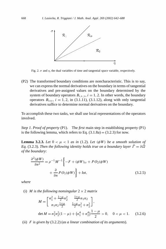
Fig. 2.σ andη, the dual variables of time and tangential space variable, respectively.

(P2) The transformed boundary conditions are noncharacteristic. This is to say,we can express the normal derivatives on the boundary in terms of tangentialderivatives and pre-assigned values on the boundary determined by thesystem of boundary operatorsBi,x,y , i = 1,2. In other words, the boundaryoperatorsBixy , i = 1,2, in (3.1.11), (3.1.12), along with only tangentialderivatives suffice to determine normal derivatives on the boundary.

To accomplish these two tasks, we shall use local representations of the operatorsinvolved.

Step 1. Proof of property(P1). Thefirst main step in establishing property (P1)is the following lemma, which refers to Eq. (3.1.8a)= (3.2.3) for now.

Lemma 3.2.3. Let 0 < µ < 1 as in (1.2). Let (φW) be a smooth solution ofEq. (3.2.3). Then the following identity holds true on a boundary layerΓ = ∂Ω

of the boundary:

∂2(φW)

∂n2 = ρ−1M−1−F + (φW)tt + PO2(φW)

+ ∂

∂nPO1(φW)

+ lot, (3.2.5)

where

(i) M is the following nonsingular2× 2 matrix

M =[n2

1+ 1−µ2 n2

21+µ

2 n1n2

n1n21+µ

21−µ

2 n21+ n2

2

],

detM = n21n

22(1−µ)+ (n4

1+ n42

)1−µ

2> 0, 0<µ< 1. (3.2.6)

(ii) F is given by(3.2.2) (as a linear combination of its arguments).

I. Lasiecka, R. Triggiani / J. Math. Anal. Appl. 269 (2002) 642–688 669

(iii) WithW =w1 dx +w2dy, see(3.1.6), we have

PO2(φW)=[c11

∂2(φw1)

∂τ2 + c12∂2(φw2)

∂τ2

c21∂2(φw1)

∂τ2 + c22∂2(φw2)

∂τ2

], (3.2.7)

PO1(φW)=[b11

∂(φw1)∂τ

+ b12∂(φw2)∂τ

b21∂(φw1)∂τ

+ b22∂(φw2)∂τ

], (3.2.8)

with coefficientsc11, . . . , b11, . . . , b22 which are given explicitly in terms ofn1, n2,µ (in the proof below), but whose exact expression is irrelevant inour present argument.

Proof. To prove (3.2.5), we return to the operator∆x,y given by (3.1.10), andexpress it exclusively in terms of normal and tangential derivatives,∂/∂n and∂/∂τ , rather than derivatives inx andy. We shall use the following identities:

∂

∂x= n1

∂

∂n− n2

∂

∂τ,

∂

∂y= n2

∂

∂n+ n1

∂

∂τ, (3.2.9)

∂2

∂x2 = n21∂2

∂n2 + n22∂2

∂τ2 − 2n1n2∂2

∂n∂τ+ lot, (3.2.10)

∂2

∂y2 = n22∂2

∂n2 + n21∂2

∂τ2 + 2n1n2∂2

∂n∂τ+ lot, (3.2.11)

∂2

∂y∂x= n1n2

∂2

∂n2− n1n2

∂2

∂τ2+ (n2

1− n22

) ∂2

∂n∂τ+ lot. (3.2.12)

Identities (3.2.9) are given, e.g., in [11, p. 299]. From these, one readily obtains(3.2.10)–(3.2.12). Next, we return to the definition of∆x,y in (3.1.10), as applied,say, toW given by (3.1.6) in terms of its coordinatesw1 andw2, substitute(3.2.10)–(3.2.12), and obtain

top row of[∆x,yW ] ≡ ∂2w1

∂x2+ 1−µ

2

∂2w1

∂y2+ 1+µ

2

∂2w2

∂y∂x

=[n2

1+(

1−µ

2

)n2

2

]∂2w1

∂n2 +[n1n2

(1+µ

2

)]∂2w2

∂n2

+[n2

2+(

1−µ

2

)n2

1

]∂2w1

∂τ2 +[−n1n2

(1+µ

2

)]∂2w2

∂τ2

+ [−n1n2(1+µ)] ∂2w1

∂n∂τ+[n2

1− n22

2(1+µ)

]∂2w2

∂n∂τ+ lot, (3.2.13)

bottom row of[∆x,yW ] ≡ 1−µ

2

∂2w2

∂x2 + ∂2w2

∂y2 + 1+µ

2

∂2w1

∂y∂x

=[n1n2

(1+µ

2

)]∂2w1

∂n2 +[(

1−µ

2

)n2

1+ n22

]∂2w2

∂n2

670 I. Lasiecka, R. Triggiani / J. Math. Anal. Appl. 269 (2002) 642–688

+[−n1n2

(1+µ

2

)]∂2w1

∂τ2 +[

1−µ

2n2

2+ n21

]∂2w2

∂τ2

+[n2

1− n22

(1+µ

2

)]∂2w1

∂n∂τ+ [n1n2(1+µ)

] ∂2w2

∂n∂τ+ lot. (3.2.14)

Thus, returning to (3.2.3), we rewrite it as

ρ∆xy(φW)=−F + (φW)tt in (0,∞)× Ω. (3.2.15)

Hence, using identities (3.2.13), (3.2.14) on the right side of (3.2.15), with theargumentW replaced by(φW), we obtain

ρ

[n2

1+ 1−µ2 n2

2 n1n21+µ

2

n1n21+µ

21−µ

2 n21+ n2

2

][ ∂2(φw1)

∂n2

∂2(φw2)

∂n2

]

=−F + (φW)tt +PO2(φW)+ ∂

∂nPO1(φW)+ lot, (3.2.16)

recalling (3.2.7), (3.2.8). Thus, (3.2.16) shows (3.2.5), by invoking the defini-tion (3.2.6) of the nonsingular matrixM and the property thatρ > 0. Lemma 3.2.3is proved.

Next, we complete the proof of property (P1), which refers to thetimelocalizationof Eq. (3.1.8a)= (3.2.3), not to (3.1.8a) itself. Letχ(t) be aC∞0time-dependent function, which is identically 1 on[α,T −α], and which vanishesoutside[α/2, T − α/2]. We then set

Wc = χW, wc = χw, χ =

1 α t T − α,0 t < α/2, t > T − α/2.

(3.2.17)

Instead of multiplying Eq. (3.1.8a)= (3.2.3) byχ(t) and repeating the argumentof Lemma 3.2.3, we prefer to multiply Eq. (3.2.5) byχ(t). This way, by (3.2.17),since∂1 in (3.1.7) is only an operator in the space variables, we obtain

∂2(φWc)

∂n2 = ρ−1M−1−F (∂1(ϕ1Wc), ∂

1(ϕ1wc))+ (φWc)tt

+ PO2(φWc)+ ∂

∂nPO1(φWc)

+ lot, (3.2.18)

where inlot in (3.2.18) we have now included also a new main term—over thelotin (3.2.5)—given by the time commutator[∂2/∂t2, χ](φW), which is first orderin t . Then (3.2.18) establishes property (P1), as desired.

Step 2. Proof of property(P2). Property (P.2) is established by the following

I. Lasiecka, R. Triggiani / J. Math. Anal. Appl. 269 (2002) 642–688 671

Lemma 3.2.4. Let 0 < µ < 1 as in (1.2). Let (φW) be a smooth solution ofEq. (3.2.3). Then the following identity holds true on the boundary∂Ω :[ ∂(φw1)

∂n

∂(φw2)∂n

]= ∂(φW)

∂n=N−1

[B1xy(φW)

B2xy(φW)

]+ PO1(φW)

, (3.2.19)

where

(i) N is the following nonsingular2× 2 matrix:

N =[ [(1−µ)ρ−1+µ]n1 [(1−µ)ρ−1+µ]n2

τ1 τ2

],

detN = (1−µ)ρ−1+µ> 0, for 0<µ< 1, (3.2.20)

τ1=−n2, τ2= n1 as in(3.1.6), τ2n1− τ1n2= τ22 + τ2

1 = 1.(ii) The operatorsBixy , i = 1,2, are given in(3.1.11), (3.1.12).

(iii) PO1(φW)=[µ[−n2

∂(φw1)∂τ

+ n1∂(φw2)∂τ

]n1

∂(φw1)∂τ

+ n2∂(φw2)∂τ

]. (3.2.21)

Proof. We return to the definition ofB1xy in (3.1.11), and expressB1xy fully interms of the normal and tangential derivatives∂/∂n and∂/∂τ : to this end, all weneed is to express this way the last divergence term in (3.1.11):

div0W = ∂w1

∂x+ ∂w2

∂y= n1

∂w1

∂n− n2

∂w1

∂τ+ n2

∂w2

∂n+ n1

∂w2

∂τ, (3.2.22)

recalling identities (3.2.9). Substituting (3.2.22) in (3.1.11) and using(φW) ratherthanW as an argument yields the top line of the following two identities, whilethe bottom line is, instead, just a rewriting ofB2xy in (3.1.12):

B1xy(φW)= [(1−µ)ρ−1+µ][n1∂(φw1)

∂n+ n2

∂(φw2)

∂n

]+µ

[−n2

∂(φw1)

∂τ+ n1

∂(φw2)

∂τ

], (3.2.23)

B2xy(φW)= ρ−1

2

τ1∂(φw1)

∂n+ τ2

∂(φw2)

∂n

+[n1∂(φw1)

∂τ+ n2

∂(φw2)

∂τ

]. (3.2.24)

Thus, (3.2.23), (3.2.24) can be rewritten as the system given by (3.2.19),with matrix N as in (3.2.20) which is nonsingular for 0< µ < 1, and termPO1(φW) given by (3.2.21). Thus, the transformed boundary conditions arenoncharacteristic. Lemma 3.2.4 is proved.

672 I. Lasiecka, R. Triggiani / J. Math. Anal. Appl. 269 (2002) 642–688

Completion of proof of Proposition 3.2.2. Having established properties (P1)and (P2) in the last two lemmas and (3.2.18), we can then assert that Proposi-tion 3.2.2 is proved on the basis of [9].Step 2. In this step we prove “half” of the desired estimate (3.2.1) of Proposi-tion 3.2.1; namely, the half involving the tangential component of∇0(φW). Moreprecisely, we shall prove

Proposition 3.2.5. Let (φW) be a smooth solution of Eq.(3.2.3). For all 0< ε <

1/2 and0< α < T/2, there existsCεα > 0 such that the following estimate holdstrue:

T−α∫α

∫Γ1

∣∣∇0(φW) · τ ∣∣2dΣ1α

Cεα

T∫0

[|Wt |20,Γ1+ |w|2

1,Ω+ |W |2

1−ε,Ω]dt

+Cε,α

∫Σ1

[∣∣g1(〈Wt,n〉

)∣∣2+ ∣∣g2(〈Wt, τ 〉

)∣∣2]dΣ1. (3.2.25)

Proof. Our starting point is estimate (3.2.4) in Proposition 3.2.2. In its right side,we substitute the feedback expressions given by (3.1.8e), (3.1.8f) for the boundaryoperatorsBixy , thus obtaining

T−α∫α

∫Γ1

∣∣∇0(φW) · τ ∣∣2dΣ1,α

Cεα

T∫0

[|Wt |20,Γ1

+ ∣∣f1((ϕ1W),g1

(〈Wt,n〉), (ϕ1w)

)∣∣20,Γ1

+ ∣∣f2((ϕ1W),g2

(〈Wt, τ 〉), (ϕ1w)

)∣∣20,Γ1

+ |F |2−1/2,Ω+ |W |2

1−ε,Ω]dt. (3.2.26)

We now recall thatf1, f2, as well asF given by (3.2.2), are all functions whichare linear combinations of their arguments, by means of smooth functions. Thus,we can estimateF in (3.2.2) recalling (3.1.7) for∂1 conservatively as

|F(t)|−1/2,Ω C[|w(t)|1,Ω + |W(t)|1−ε,Ω

], 0< ε <

1

2, (3.2.27)

I. Lasiecka, R. Triggiani / J. Math. Anal. Appl. 269 (2002) 642–688 673

and apply trace theory to the terms|(ϕ1W)|0,Γ1and|(ϕ1w)|0,Γ1

coming fromfi ,to obtain (3.2.25) from (3.2.26) and (3.2.27), as desired.Remark 3.2.1. Estimate (3.2.25), when applied to thehomogeneous system ofdynamic elasticity, states that the traces of the tangential derivatives ofW arebounded by the traces of velocity modulo lower-order terms. A result of similarnature was obtained first for the classical wave equation in [8].

Step 3. In this step, we prove the second “half” of the desired final estimate(3.2.1) of Proposition 3.2.1; namely, the half involving the normal componentof ∇0(φW). More precisely, we shall prove

Proposition 3.2.6. Let (φW) be a smooth solution of Eq.(3.2.3). For all 0< ε <

1/2 and0< α < T/2, there existsCεα > 0 such that the following estimates holdtrue:

(i)

T−α∫α

∫Γ1

∣∣∇0(φW) · n∣∣2dΣ1,α Cεα

T−α∫α

∫Γ1

∣∣∇0(φW) · τ ∣∣2 dΣ1α

+Cεα

∫Σ1

[∣∣g1(〈Wt ,n〉

)∣∣2+ ∣∣g2(〈Wt, τ 〉

)∣∣2]dΣ1

+Cεα

T∫0

[|w|21,Ω

+ |W |21−ε,Ω]dt. (3.2.28)

(ii) From (3.2.25)and(3.2.28), we obtain

T−α∫α

∫Γ1

∣∣∇0(φW) · n∣∣2dΣ1,α

Cεα

T∫0

[|Wt |20,Γ1+ |w|2

1,Ω+ |W |2

1−ε,Ω]dt

+Cεα

∫Σ1

[∣∣g1(〈Wt,n〉

)∣∣2+ ∣∣g2(〈Wt , τ 〉

)∣∣2]dΣ1. (3.2.29)

Proof. (i) Recalling, again, the feedback expressions (3.1.8d), (3.1.8e) for theboundary operatorsBixy , and the definition ofPO1(φW) in (3.2.21), we estimate

674 I. Lasiecka, R. Triggiani / J. Math. Anal. Appl. 269 (2002) 642–688∣∣∣∣[B1xy(φW)

B2xy(φW)

]+ PO1(φW)

∣∣∣∣0,Γ1

=∣∣∣∣∣f1((ϕ1W),g1

(〈Wt ,n〉), (ϕ1w)

)+µ

[−n2

∂(φw1)

∂τ+ n1

∂(φw2)

∂τ

]∣∣∣∣∣0,Γ1

+∣∣∣∣∣f2((ϕ1W),g2

(〈Wt, τ 〉), (ϕ1w)

)+[n1∂(φw1)

∂τ+ n2

∂(φw2)

∂τ

]∣∣∣∣∣0,Γ1

(3.2.30)

∣∣∇0(φW) · τ ∣∣0,Γ1

+ |w|1,Ω + |W |1−ε,Ω +∣∣g1(〈Wt,n〉

)∣∣0,Γ1

+ ∣∣g2(〈Wt, τ 〉

)∣∣0,Γ1

. (3.2.31)

In going from (3.2.30) to (3.2.31), we have recalled once more thatf1 andf2are linear combinations of their arguments by means of smooth functions, and wehave used trace theory on|(ϕ1w)|0,Γ1

and|(ϕ1W)|0,Γ1. Inserting estimate (3.2.30)

into the right side of (3.2.19) and integrating over(α,T − α) × Γ1 yields esti-mate (3.2.28), as desired.

(ii) We substitute the tangential component of∇0(φW), given by (3.2.25),into the right side of inequality (3.2.28), and finally obtain estimate (3.2.29).Proposition 3.2.6 is proved.Step 4. We now combine the last two propositions to obtain the desired finalestimate of∇0(·) on the boundary, at least in the argument(φW).

Proposition 3.2.7. Let (φW) be a smooth solution of Eq.(3.2.3). For all 0< ε <

1/2 and0< α < T/2, there existsCεα > 0 such that the following estimate holdstrue:

T−α∫α

∫Γ1

∣∣∇0(φW)∣∣2dΣ1α

Cεα

∫Σ1

[|Wt |2+

∣∣g1(〈Wt,n〉

)∣∣2+ ∣∣g2(〈Wt , τ 〉

)∣∣2]dΣ1

+Cεα

T∫0

[|w(t)|21,Ω

+ |W(t)|21−ε,Ω]dt. (3.2.32)

I. Lasiecka, R. Triggiani / J. Math. Anal. Appl. 269 (2002) 642–688 675

Proof. We combine estimate (3.2.25) of Proposition 3.2.5 with estimate (3.2.29)of Proposition 3.2.6, to obtain estimate (3.2.32) at once.Step 5. Conclusion of the proof of Theorem 3.2.1.Recalling the partition of unity(3.1.4), we add all the estimates (3.2.32) for all finitely manyφ and obtain thedesired estimate (3.2.1) of Proposition 3.2.1.3.3. Trace regularity for normal componentw

Our next result deals with the improved trace regularity for the normal dis-placementw.

Proposition 3.3.1. Let W,w be a finite energy solution to problem(1.1) asguaranteed by Theorem1.1. Then, there is a constantCαT ε > 0 such that

T−α∫α

∫Γ1

|D2w|2T 2xdΣ1α

C

∫Σ1

[|Dwt |2+

∣∣∣∣h1

(∂wt

∂n

)∣∣∣∣2+ ∣∣∣∣h2

(∂wt

∂τ

)∣∣∣∣2]dΣ1

+T∫

0

[|w(t)|22−ε,Ω + |wt(t)|21−ε,Ω + |W(t)|21−ε,Ω]dt

. (3.3.1)

Proof. As before, it suffices to prove this estimate locally in a layer of theboundaryΓ of Ω for solutions supported in supp ofφ.

Step 1. Define

G(x, y, t)≡ G(∂1(ϕ1W),∂3(ϕ1w)

), (3.3.2)

f3(x, y, t)≡ f3

(∂1(ϕ1w),h1

(∂wt

∂n

)), (3.3.3)

f4(x, y, t)≡ f4

(∂2(ϕ1w),wtt ,

∂

∂τh2

(∂

∂τwt

)), (3.3.4)

in the notation (3.1.7) for∂& as a general differential operator of order& in thespace variablesx andy, whereG, as well asf3 andf4, are linear combinations oftheir arguments, by means of smooth functions. As such,G, f3, f4 are Nemytskioperators. With the above notation, the variable(φw) satisfies Eq. (3.1.8b), alongwith the corresponding boundary conditions (3.1.8f) and (3.1.8g). We rewrite herethe corresponding linear Kirchhoff plate problem in(φw), where the right side

676 I. Lasiecka, R. Triggiani / J. Math. Anal. Appl. 269 (2002) 642–688

operatorG in (3.1.8b) is rewritten here in the formG= G+O((∂/∂t)∂1(ϕ1wt))

—with G as in (3.3.2)—to distinguish it between space and time derivatives.Thus,(φw) satisfies

(φw)tt − γρ∆0(φw)tt + ρ2γ∆20(φw)=G

= G+O(ddt∂1(ϕ1wt)

), (3.3.5a)

∂2

∂n2 (φw)+µ ∂2

∂τ2 (φw)= f3, (3.3.5b)

∂3

∂n3 (φw)+ ∂∂n

∂2

∂τ2 (φw)+ (1−µ) ∂2

∂τ2∂∂n(φw)

− γ ∂∂n(φw)tt = f4, (3.3.5c)

wheref3 andf4 are given by (3.1.8f) and (3.1.8g). To problem (3.3.5a), (3.3.5b)we apply [10, p. 279, Theorem 2.1], which gives an improved trace regularityestimate. We obtain

T−α∫α

∫Γ1

∣∣D2(φw)∣∣2dΣ1α

C

T−α∫α

∫Γ1

[∣∣∣∣∂2(φw)

∂τ2

∣∣∣∣2+ ∣∣∣∣∂2(φw)

∂n2

∣∣∣∣2+ ∣∣∣∣∂2(φw)

∂τ∂n

∣∣∣∣2]dΣ1α (3.3.6)

C

∫Σ1

|∇0wt |2dΣ1+T∫

0

[|G(t)|2

(H3/2(Ω))′ +∣∣∂1(φ(wt )

)(t)∣∣2−1/2+ε,Ω

+ |w(t)|22−ε,Ω]dt + |f3|20,Σ1

+ |f4|2−1,Σ1

, (3.3.7)

recalling the boundary conditions (3.3.5b). The first estimate in (3.3.6) followsfrom the definition of norm ofD2w(·, ·) given in (A.1) and (A.2).

Remark 3.3.1. Estimate (3.3.7) for the Kirchhoff plate problem (3.3.5) is liftedfrom [11, p. 279, Theorem 2.1], except that we are giving in (3.3.7) a sharper resultfor the right-hand sideG in (3.3.5a). This calls for an explanation. The resultgiven in [11, Theorem 2.1] penalizes the “right-hand side” termG in the normof H−s , s < 1/2, in time and space. However, a sharper regularity result may begiven onG, if one distinguishes between tangential and normal directions. (Thisexplains why we have rewrittenG asG= G+O((∂/∂t)∂1(ϕ1wt)), to distinguishbetween space and time derivatives.) More precisely, restrictions on the regularityof the forcing termG in (3.3.5) are dictated by the applicability of elliptic theoryin an “elliptic sector” (see [10]). In our case, the Kirchhoff plate equation (3.3.5a)is supplemented with the free boundary conditions (3.3.5b) and (3.3.5c). IfL

denotes the realization inL2(V ) of ∆20 with the free B.C. (3.3.5b) and (3.3.5c),

I. Lasiecka, R. Triggiani / J. Math. Anal. Appl. 269 (2002) 642–688 677

thenL is positive, self-adjoint, andD(Ls/4) = Hs(V ), s < 5/2 [11, Chapter 3,Appendix B]. Thus, we have been conservative in (3.3.7) onG. Moreover, themicrolocal argument in [10] is applied to functions with compact support in[0, T ]in time: thus, all boundary terms produced by integration by parts in time vanish.In conclusion, the termG in (3.3.5a), when viewed as forcing term on the right-hand side of the elliptic equation in an “elliptic sector,” may be allowed to lie in aspace which is dual toHs,0(V × [0, T ]), s < 5/2:G ∈ [Hs,0(V × [0, T ])]′.

HereHs,0(V × [0, T ]) is the completion in theHs(V × [0, T ])-norm of allC∞(V × [0, T ])-functions which vanish outside[α,T − α] in the t-direction.Thus, our estimate forG in (3.3.7) is still conservative, though explicitly notcontained in [11, Theorem 2.1].

Step 2. We estimate next the contribution of the termsG, f3, f4 in (3.3.7).

Lemma 3.3.2. Let W,w be a regular solution of problem(1.1). Then, for allε < 1/2 the following estimates hold:

(i)

|G(t)|(H3/2(Ω))′ C|w(t)|2−ε,Ω + |W(t)|1−ε,Ω + |f3(t)|0,Γ1, (3.3.8)

(ii)

|f3|0,Σ1C

[∣∣∣∣h1

(∂

∂nwt

)∣∣∣∣0,Σ1

+[ T∫

0

|w(t)|22−ε,Ω dt

]1/2], (3.3.9)

(iii)

|f4(t)|2−1,Σ1C

T∫0

[∣∣∣∣h2

(∂wt(t)

∂τ

)∣∣∣∣20,Γ1

+∣∣∣∣h1

(∂wt(t)

∂n

)∣∣∣∣2

+ |wt |20,Γ1+ |w|2

2−ε,Ω

]dt. (3.3.10)

Proof. (i) For the proof of (3.3.8), we shall use duality. Letψ ∈H 3/2(Ω). Then,using the definition (3.3.2) ofG (as a linear combination of its arguments bymeans of smooth functions), we obtain∣∣(G(t),ψ)

Ω

∣∣C∣∣(∂1(ϕ1W),ψ

)Ω

∣∣+ ∣∣(∂3(ϕ1w),ψ)Ω

∣∣C|W |1−ε,Ω |ψ|ε,Ω +

∣∣(∂3(ϕ1w),ψ)Ω

∣∣. (3.3.11)

678 I. Lasiecka, R. Triggiani / J. Math. Anal. Appl. 269 (2002) 642–688

Regarding the first term in (3.3.11), writing∂1= div0,x,y + lot, and applyingthe divergence theorem and accounting for the boundary conditions (3.3.5b), weobtain, recalling suppϕ1⊂ suppφ by Lemma 3.1.2 below (3.1.9),(

∂3(ϕ1w),ψ)Ω

C∣∣(∂2(ϕ1w), ∂

1ψ)Ω

∣∣+ ∣∣∣∣( ∂2

∂n2 (ϕ1w),ψ

)Γ1

∣∣∣∣(by (3.3.5b))

C

∣∣(∂2(ϕ1w), ∂1ψ)Ω

∣∣+ ∣∣∣∣( ∂2

∂τ2 (ϕ1w),ψ

)Γ1

∣∣∣∣+ ∣∣(f3,ψ)Γ1

∣∣ C|ϕ1w|2−ε,Ω |∂1ψ|ε,Ω +C|ϕ1w|1,Γ1

|ψ|1,Γ1 +C|f3|0,Γ1|ψ|0,Γ1

C[|w|2−ε,Ω |ψ|3/2,Ω + |f3|0,Γ1|ψ|1,Ω

], (3.3.12)

where in the last steps we have also used trace theory on|(ϕ1w)|1,Γ1and|ψ|0,Γ1

.Combining (3.3.11) and (3.3.12) proves the first estimate (3.3.8) in part (i).(ii) As to the proof of the second part, estimate (3.3.9), the argument is simpler

and uses only trace theory: recallingf3 in (3.3.3), we have

|f3|0,Σ1C∣∣∂1(ϕ1w)

∣∣0,Σ1

+C

∣∣∣∣h1

(∂wt

∂n

)∣∣∣∣0,Σ1

C

[∣∣∣∣h1

(∂wt

∂n

)∣∣∣∣0,Σ1

+[ T∫

0

|w|22−ε,Ω dt

]1/2], (3.3.13)

and (3.3.9) in part (ii) is proved.(iii) We now prove estimate (3.3.10). Recallingf4 in (3.3.4), we estimate

|f4(t)|−1,Σ1C

[∣∣∂2(ϕ1w)∣∣−1,Σ1

+ |wtt |−1,Σ1+∣∣∣∣ ∂∂τ h2

(∂wt

∂τ

)∣∣∣∣−1,Σ1

]

C

[∣∣∂2(ϕ1w)∣∣−1,Σ1

+ |wt |0,Σ1+∣∣∣∣h2

(∂wt

∂τ

)∣∣∣∣0,Σ1

]

C

[∣∣∣∣ ∂2

∂n2 (ϕ1w)

∣∣∣∣−1,Σ1

+ ∣∣∂1(ϕ1w)∣∣0,Σ1

+∣∣∣∣h2

(∂wt

∂τ

)∣∣∣∣0,Σ1

+ |wt |0,Σ1

]

C

[∣∣∣∣ ∂2

∂n2(ϕ1w)

∣∣∣∣−1,Σ1

+[ T∫

0

|w|22−ε,Ω dt

]1/2

I. Lasiecka, R. Triggiani / J. Math. Anal. Appl. 269 (2002) 642–688 679

+∣∣∣∣h2

(∂wt

∂τ

)∣∣∣∣0,Σ1

+ |wt |0,Σ1

]. (3.3.14)

The second normal derivatives terms in (3.3.14) can be eliminated by usingboundary conditions for the boundary moments: to this end, we invoke (3.3.5b)and recall that suppϕ1⊂ suppφ (see below (3.1.9)). We thus obtain via (3.3.3)∣∣∣∣ ∂2

∂n2(ϕ1w)

∣∣∣∣−1,Γ1

C

[∣∣∣∣ ∂2

∂τ2ϕ1w

∣∣∣∣−1,Γ1

+∣∣∣∣f3

(∂1(ϕ1w),h1

(∂wt

∂n

))∣∣∣∣−1,Γ1

](3.3.15)

C

[|ϕ1w|1,Γ1

+ ∣∣∂1(ϕ1w)∣∣0,Γ1

+∣∣∣∣h1

(∂wt

∂n

)∣∣∣∣0,Γ1

](3.3.16)

C

[|w|2−ε,Ω +

∣∣∣∣h1

(∂wt

∂n

)∣∣∣∣0,Γ1

], 0< ε <

1

2, (3.3.17)

whereϕ2 in (3.3.15) is a smooth function with support larger than the supportof ϕ1: suppϕ1⊂ suppϕ2; the passage from (3.3.15) to (3.3.16) is based on crudeestimate; finally, the last step from (3.3.16) to (3.3.17), we have used trace theoryon |w|1,Γ1

and|Dw|0,Γ1. Substituting (3.3.17) into the right-hand side of (3.3.14)

proves estimate (3.3.10) of part (iii). Lemma 3.3.2 is proved.Step 3. We substitute inequalities (3.3.8)–(3.3.10) forG, f3, f4 into the rightside of (3.3.7), and sum up all such resulting estimates with respect to thepartition of unity as in (3.1.4) forw, and obtain the sought-after estimate (3.3.1).Proposition 3.3.1 is thus proved.3.4. Completeness of proof of Theorem 3.1.1

Finally, we combine estimate (3.2.1) onW in Proposition 3.2.1 with esti-mate (3.3.1) onw in Proposition 3.3.1. This way, we obtain the desired in-equality (3.1.3) and hence the desired inequality (3.1.1). Theorem 3.1.1 is thusproved.

4. Stabilizability estimate and completion of the proof of Theorem 1.2

The remaining part of the proof of Theorem 1.2 is contained (as a strict subset)in the arguments presented in [19] (see also [32]). For the reader’s convenience,we shall outline the remaining steps.

680 I. Lasiecka, R. Triggiani / J. Math. Anal. Appl. 269 (2002) 642–688

Step 1. We proceed as in [8, Section 7.3] and [19]. We return to estimate (2.4)of Proposition 2.2, this time over the interval[α,T − α] rather than over[0, T ]. On the left-hand side, we obtain(T − 2α)E(T )

∫ T−αα E(t) dt by the

dissipativity property in (2.1). On the right-hand side, we use: (i) estimate (3.1.1)of Theorem 3.1.1 for the boundary termsBTbad[α,T − α] over [α,T − α];(ii) identity (2.1) again withs = 0, t = T , to expressE(0) in terms ofE(T ) plusboundary terms, where we use 2gi(s)s |gi(s)|2 + s2, 2hi(s)s |hi(s)|2 + s2

for these boundary terms, as well as (A.1), (A.2) to estimate them by the normsof Dwt andWt . This way, using again (2.4), we readily obtain the counterpartof [19, Lemma 3.3].

Proposition 4.1. With reference to the energy in(1.17), the strong solutions ofthe original dynamics(1.1), guaranteed by Theorem1.1, satisfy the followingestimate for allT > 0 sufficiently large: there is a constantCT > 0 such that

E(T )+T∫

0

E(t) dt

CT

∫Σ1

‖Wt‖2

L2(Γ,Λ)+ ‖Dwt‖2

L2(Γ,Λ)+ ∣∣g1(〈Wt,n〉

)∣∣2+ ∣∣g2(〈Wt, τ 〉

)∣∣2+ ∣∣∣∣h1

(∂wt

∂n

)∣∣∣∣2+ ∣∣∣∣h2

(∂wt

∂τ

)∣∣∣∣2dΣ1

+ LOT(W,w), (4.1)

where, as before, LOT(W,w) are lower terms(with respect to the energy) asdefined in(3.1.2c).

Step 2. Lower-order terms are absorbed, as usual, by a compactness/uniquenessargument. This requires an appropriate unique continuation result (from theboundary). Since the coefficients are time-independent, it is far convenient torequire a uniqueness result for the corresponding static problem. The latter isestablished in [3, Proposition 2.3], by reducing the Cauchy problem to a systemof three equations of the fourth order with the same principal part∆2, where∆ isthe Laplacian on the manifoldM. For this latter problem, the result in [28] is theninvoked to obtain uniqueness. (One could also use results of [27]). Thus, a by-now standard compactness/uniqueness argument (see [19, Lemma 4.1]) leads tothe absorption of lower-order terms. We thus obtain

Lemma 4.2. With reference to the LOT(W,w) in estimate(4.1) for the strongsolutions of problem(1.1), there existsT > 0 large enough, so that

I. Lasiecka, R. Triggiani / J. Math. Anal. Appl. 269 (2002) 642–688 681

LOT(W,w)≡T∫

0

[|W(t)|21−ε,Ω + |w(t)|22−ε,Ω]dt

CT

∫Σ1

[|Wt |2+ |Dwt |2+

∣∣g1(〈Wt,n〉

)∣∣2+ ∣∣g2(〈Wt , τ 〉

)∣∣2+∣∣∣∣h1

(∂wt

∂n

)∣∣∣∣2+ ∣∣∣∣h2

(∂wt

∂τ

)∣∣∣∣2]dΣ1. (4.2)

Step 3. By combining the results of Proposition 4.1 and Lemma 4.2, we obtainthe final stabilization estimate.

Proposition 4.3. Let [W,w] be a regular solution to the original system(1.1), asguaranteed by Theorem1.1. Then, there exists a constantT0 > 0 such that for anyT > T0, there is a constantCT > 0 such that the following estimate holds true:

E(0)+E(T )+T∫

0

E(t) dt

CT

∫Σ1

[|Wt |2+ |Dwt |2+

∣∣g1(〈Wt,n〉

)∣∣2+ ∣∣g2(〈Wt , τ 〉

)∣∣2+∣∣∣∣h1

(∂wt

∂n

)∣∣∣∣2+ ∣∣∣∣h2

(∂wt

∂τ

)∣∣∣∣2]dΣ1. (4.3)

Step 4. Our next step is to express the boundary terms in terms of the feedbacksin (1.1d)–(1.1f). To accomplish this, we shall use the growth conditions (1.26)imposed on the nonlinear dissipation termsgi , hi at infinity, together with theconsequent properties (1.29) of the “comparison” functionsgi , hi which containinformation on the growth at the origin. It isonly at this pointthat we use thegrowth conditions(1.26) imposed on the nonlinear functionsgi , hi given inassumption (H.3)= (1.26), together with the construction of the functionsgi ,hi which capture the behavior of the nonlinearity at the origin.

By splitting the integration on the boundary between “low” and “high” fre-quencies, and using Jensen’s inequality in the same manner as it is used on [19,pp. 1400–1401], we arrive at the following conclusion.

Proposition 4.4. Consider regular solutions of problem(1.1), as guaranteed byTheorem1.1. LetE(t) be defined in(1.17). Then there existsT > 0 such that

p(E(T ))+E(T )E(0), (4.4)

where the monotone functionp is defined constructively in(1.31).

682 I. Lasiecka, R. Triggiani / J. Math. Anal. Appl. 269 (2002) 642–688

Step 5. The final conclusion of Theorem 1.2 now follows from (4.4) and [19,Lemma 3], which is based on a comparison theorem.

Appendix A. Middle surface as a Riemann manifold with the inducedmetric of R3

That given in (1.1) of Section 1 is the classical shallow shell model, however,in a version produced in [2,3], in which the middle surface is viewed as aRiemann manifold with the induced metric ofR3. This contrasts with the classicalapproach, where the middle surface is instead the image, under a smooth map,of a two-dimensional connected domain, and therefore described under just onecoordinate patch. The Riemann geometric view of the middle surface, while muchmore flexible and general than the classical approach, requires, however, a heavydifferential geometric setting and apparatus. This is given here for the purposeof explaining the quantities entering model (1.1) and providing the necessarybackground for the analysis of the shell.

A.1. Riemann geometric background and notation

We reproduce here from [2,3] the Riemann geometric background indispensi-ble to obtain and understand model (1.1) of the shell, with middle surface viewedas a Riemann manifold. See [24–26,29,30].

(1) The usual inner product (dot product) inR3 is denoted by〈·, ·〉. LetM bea smooth, orientable surface inR3 with unit normal fieldN(x), x ∈M. We viewM as a 2-dimensional Riemann manifold with metric induced fromR3, whichwill be denoted byg(·, ·) or 〈·, ·〉, as convenient. For eachx ∈M, Mx denotes the(2-dimensional) tangent space ofM at x. We denote: the set of all vector fieldson M by X (M); the set of allk-order tensors onM by T k(M); and the set ofall k-forms onM by Λk(M), respectively, for any nonnegative integerk. ThenΛ0(M)= T 0(M)= C∞(M)= the set of allC∞-functions onM; moreover,

T 1(M)= T (M)=Λ(M)=X (M), (A.0)

whereΛ(M)=X (M) has to be interpreted as the following isomorphism: givenX ∈X (M); thenU(Y )= 〈Y,X〉, ∀Y ∈ X (M) determines a uniqueU ∈Λ(M).

(2) For eachx ∈M, the k-order tensor spaceT kx on M is an inner product

space whose inner product is defined as follows. Let[e1, e2] be an orthonormalbasis ofMx . For any twok-order tensorsα,β ∈ T k

x , x ∈ M, define the innerproduct ofT k

x by

〈α,β〉T kx=

2∑i1,...,ik=1

α(ei1, . . . , eik )β(ei1, . . . , eik ) atx. (A.1a)

I. Lasiecka, R. Triggiani / J. Math. Anal. Appl. 269 (2002) 642–688 683

In particular, fork = 1, definition (A.1a) becomes

〈α,β〉T kx= 〈α,β〉 = g(α,β), ∀α,β ∈Mx, (A.1b)

and we obtain the inner product ofMx induced byR3.(3a) LetΩ be a bounded region of the surfaceM with boundaryΓ which

is either regular or else empty. By (A.1),T k(Ω) are inner product spaces in thefollowing sense: the inner product is defined by

(T1, T2)T k(Ω) ≡∫Ω

〈T1, T2〉T kxdx, T1, T2 ∈ T k(Ω), (A.2)

using (A.1), wheredx is the “volume element” of the surfaceM with respect toits Riemann metricg [30, p. 30].

(3b) We denote byL2(Ω,T k) the space which is the completion ofT k(Ω)

with respect to the inner product (A.2). In particular, via (A.0), we have thatL2(Ω,Λ)= L2(Ω,T ).

(4) The spaceL2(Ω) is the completion ofC∞(Ω)with respect to the followinginner product:

(f,h)L2(Ω) =∫Ω

f (x)h(x) dx, f,h ∈C∞(Ω). (A.3)

(5) LetD denote the Levi-Civita connection onM in the metricg ofM inducedfrom R3 [24,29,30].

(5a) For a vector fieldU ∈ X (M), DU ∈ T 2(M) denotes the covariant dif-ferential ofU : it is a second-order covariant tensor field (bilinear map) definedby

DU(X,Y )= 〈DYU,X〉 =DYU(X), ∀X,Y ∈Mx, x ∈M. (A.4)

One similarly defines the second-order covariant tensor fieldD∗U ∈ T 2(M)

by

D∗U(X,Y )=DU(Y,X), ∀X,Y ∈Mx, x ∈M, (A.5)

so thatD∗U is the transpose ofDU in T 2(M).(5b) Letf ∈ C2(M). By definition, the HessianD2f of f with respect to the

metricg is of second-order tensor defined by

D2f (X,X)= ⟨DX(Df ),X⟩. (A.6)

(6) For any second-order tensorT ∈ T 2(M), the trace ofT atx ∈M is definedby

trT =2∑

i=1

T (ei , ei) ∈ C∞(M), (A.7)

where[e1, e1] is an orthonormal basis ofMx with respect tog.

684 I. Lasiecka, R. Triggiani / J. Math. Anal. Appl. 269 (2002) 642–688

(7) LetDk be thekth covariant differential off in the induced metricg of M,wheref ∈ C∞(Ω). ThenDkf is a k-order tensor field onΩ and‖ · ‖L2(Ω,T k)

and ‖ · ‖L2(Ω) are the norms induced by the inner products (A.2) and (A.3),respectively. Then, the Sobolev spaceHn(Ω) is the completion ofC∞(Ω) withrespect to the norm

‖f ‖Hn(Ω) =

n∑k=1

‖Dkf ‖2L2(Ω,T k)

+ ‖f ‖2L2(Ω)

1/2

. (A.8)

For details on Sobolev spaces on Riemann manifolds, we refer to [31] or [24].(8) The Sobolev spaceHk(Ω,Λ) and its inner product are defined by

Hk(Ω,Λ)= U : U ∈ L2(Ω,Λ), DiU ∈ L2(Ω,T i+1),

i = 1, . . . , k, (A.9)

(U,V )Hk(Ω,Λ) =k∑

i=0

(DiU,DiV )L2(Ω,T i+1),

∀U,V ∈Hk(Ω,Λ). (A.10)

In particular,H 0(Ω,Λ)= L2(Ω,Λ).

(9a) The Lie bracket[X,Y ] of two vector fieldsX andY is the vector fielddefined by

[X,Y ](f )=X[Y (f )] − Y [X(f )], (A.11)

wheref is aC2 function onM.(9b) The exterior derivative

d :Λk(M)→Λk+1(M) (A.12)

is defined as follows [29, p. 53]: Letη ∈Λk(M); then

dη(X1, . . . ,Xk+1)

=k+1∑i=1

(−1)i−1Xi

[η(X1, . . . , Xi, . . . ,Xk+1)

]+∑i<j

(−1)i+j η([Xi,Xj ],X1, . . . , Xi , . . . , Xj , . . . ,Xk+1

), (A.13)

whereX1, . . . ,Xk+1 are vector fields. A caret over a term means that this term isomitted. According to this definition, we have:

(i)

f ∈Λ0(M) ⇒ df (X)=X(f )= 〈Df,X〉. (A.14)

I. Lasiecka, R. Triggiani / J. Math. Anal. Appl. 269 (2002) 642–688 685

(ii)

η ∈Λ1(M)

⇒ dη(X,Y )=X[η(Y )] − Y [η(X)] − η([X,Y ]). (A.15)

(iii) (Local expression of the exterior differential) Let(Ω,φ) be a local chart,x1, . . . , xn the corresponding coordinates onΩ , ∂/∂xi, i = 1, . . . , n, thenvector fields of the natural basis, anddxi the dual basis. The differentialk-form η is written as ([24, p. 63], [29, p. 53])

η=∑

j1<j2<···<jkaj1...jk (x) dx

j1 ∧ · · · ∧ dxjk , (A.16)

whereaj1...jk are differentiable real-valued functions. Then ([24, p. 66], [29,p. 54]),

dη=∑

j1<j2<···<jkdaj1...jk ∧ dxj1 ∧ · · · ∧ dxjk , (A.17)

da denoting the differential of the scalar functiona. From this expression,we see that ([24, p. 67], [26, p. 183], [29, p. 54]),

d(η∧ ξ)= dη ∧ ξ + (−1)kη ∧ dξ, (A.18)

and then

d2= d d = 0. (A.19)

(10) There is a first-order differential operator [24, p. 162]

δ :Λk+1(Ω)→Λk(Ω) (A.20)

which is the formal adjoint ofd , and is characterized by

(dα,β)L2(Ω,Λk+1) = (α, δβ)L2(Ω,Λk) for α ∈Λk(Ω), β ∈Λk+1(Ω),

(A.21)

with compact support. We set

δ = 0 on 0-forms. (A.22)

Formula (A.22) implies

δ2= 0, (A.23)

δ on 1-forms [24, p. 164]. LetX be a vector field andω be the 1-form corre-sponding toX under the given metricg: g(Y,X) = 〈Y,ω〉; see point (1) aboveΛ(M)=X (M). Then [24, p. 164]

δω=−divX. (A.24)

686 I. Lasiecka, R. Triggiani / J. Math. Anal. Appl. 269 (2002) 642–688

This identity is equivalent to

(X,gradu)L2(M) =−(divX,u)L2(M),

and the definition ofδ as the formal adjoint ofd .Moreover, ifω is a 2-form inR2 of the typeω = f dx ∧ dy [as in (3.1.33),

(3.1.34)], then [26, p. 228]

δ0ω =−∂f

∂xdy + ∂f

∂ydx. (A.25)

(11) The Hodge Laplacian operator onk-forms

∆ :C∞(Ω,Λk)→ C∞(Ω,Λk) (A.26)

is defined by ([24, p. 162], [26, p. 226, with opposite sign])

−∆= (d + δ)2= dδ+ δd, (A.27)

recalling (A.23) and (A.19). Consequently,

A.28(−∆u,v)L2(Ω,Λk) = (du, dv)L2(Ω,Λk+1) + (δu, δv)L2(Ω,Λk−1)

for u,v ∈C∞0 (Ω,Λk). (A.28)

Sinceδ = 0 onΛ0(Ω), see (A.22), we have

−∆= δd onΛ0(Ω). (A.29)

A.2. Shell

(a) A shell is a body inR3. Assume that the middle surface of the shell occupiesa bounded regionΩ of the smooth orientable surfaceM in R3. Then the shell ofthicknessh > 0 (“small”) is defined by

S =p: p = x + zN(x), x ∈Ω, −h

2< z <

h

2

. (A.30)

HereN(x) is the unit normal field onΩ .(b) The second fundamental formΠ of M is the 2-covariant tensor, defined by

Π(X,Y )= 〈DXN,Y 〉, ∀X,Y ∈ X (M), (A.31)

whereD is the covariant differential ofR3 in the usual dot product. For any vectorfieldsX,Y onM, since the manifoldM is the submanifold ofR3, we then obtain

DXY =DXY + 〈DXY,N〉N =DXY −Π(X,Y )N,

whereD is the covariant differential of the surfaceM with respect to the metricg.(c) The mean curvatureH of the surfaceM and the Gaussian curvatureκ are

given by ([2, (3.1.31)], [30, p. 142])

κ = κ1, κ2, H = trΠ = κ1+ κ2, (A.32)

whereκ1, κ2 are the principal curvatures.

I. Lasiecka, R. Triggiani / J. Math. Anal. Appl. 269 (2002) 642–688 687

References

[1] C. Bardos, G. Lebeau, J. Rauch, Sharp sufficient conditions for the observation, control, andstabilization of wave from the boundary, SIAM J. Control Optim. 30 (1992) 1024–1065.

[2] P.F. Yao, On shallow shell equations, manuscript (1999).[3] P.F. Yao, Observability inequalities for shallow shells, SIAM J. Control 38 (2000) 1729–1756.[4] J. Lagnese, Boundary Stabilization of Thin Plates, SIAM, 1989.[5] J. Puel, M. Tucsnak, Boundary stabilization for the von Karman equations, SIAM J. Control 33

(1996) 255–273.[6] I. Lasiecka, Uniform stabilizability of a full von Karman system with nonlinear boundary

feedback, SIAM J. Control 36 (1998) 1376–1422.[7] I. Lasiecka, Uniform decay rates for the full von Karman system of dynamic thermo-elasticity

with free boundary conditions and partial dissipation, Comm. Partial Differential Equations 24(1999) 1801–1849.

[8] I. Lasiecka, R. Triggiani, Uniform stabilization of the wave equation with Dirichlet and Neumannfeedback control without geometrical conditions, Appl. Math. Optim. 25 (1992) 189–224.

[9] M.A. Horn, Sharp trace regularity of the traces to solution of dynamic elasticity, J. Math. SystemsEstim. Control.

[10] I. Lasiecka, R. Triggiani, Sharp trace estimates of solutions to Kirchhoff and Euler Bernoulliequations, Appl. Math. Optim. 28 (1993) 277–306.

[11] I. Lasiecka, R. Triggiani, Control Theory for Partial Differential Equations, Vol. 1, CambridgeUniversity Press, 2000.

[12] J. Lagnese, Modeling and stabilization of nonlinear plates, Internat. Ser. Numer. Math. 100(1991) 247–264.

[13] J. Lagnese, Uniform asymptotic energy estimates for solutions of the equations of dynamic planeelasticity with nonlinear dissipation of the boundary, Nonlinear Anal. 16 (1991) 35–54.

[14] V. Barbu, Nonlinear Semigroups and Differential Equations in Banach Space, Noordhoff, 1976.[15] I. Lasiecka, Mathematical Control Theory of Coupled Systems, Lecture Notes CMBS-NSF,

SIAM, 2001.[16] I. Lasiecka, R. Marchand, Uniform decay for solutions to nonlinear shells with nonlinear

dissipation, Nonlinear Anal. 30 (1997) 5409–5418.[17] M. Bernadou, J.M. Boisserie, The Finite Element Method in Thin Shell Theory: Applications to

Arch Dam Simulation, Progress in Scientific Computing, Vol. 1, Birkhäuser, Boston, 1982.[18] M. Bernadou, J.T. Oden, An existence theorem for a class of nonlinear shallow shell problems,

J. Math. Pures Appl. 60 (1981) 258–298.[19] I. Lasiecka, D. Tataru, Uniform boundary stabilization of semilinear wave equations with

nonlinear boundary damping, Differential Integral Equations 6 (1993) 507–533.[20] S. Chai, Y. Guo, P. Yao, Uniform stabilization of a shallow shell by boundary dissipation,

manuscript (2001).[21] I. Lasiecka, R. Triggiani, W. Valente, Uniform stabilization of spherical shells by boundary

dissipation, Adv. Differential Equations 1 (1996) 635–674.[22] I. Lasiecka, W. Valente, Uniform boundary stabilization of a nonlinear shallow and tin spherical

cap, J. Math. Anal. Appl. 22 (1996) 951–994.[23] R. Schoen, S.T. Yau, Lectures on Differential Geometry, International Press, 1994.[24] M. Taylor, Partial Differential Equations, I, Springer, 1996.[25] G. Gentili, F. Podestá, E. Vesentini, Lezioni di Geometria Differenziale, Boringhieri, 1995.[26] J.T. Wloka, B. Rowley, B. Lawruk, Boundary Value Problems for Elliptic Systems, Cambridge

University Press, 1995.[27] L. Hormander, The Analysis of Linear Partial Differential Operators, I–IV, Springer, 1985.[28] T. Shirota, A remark on the unique continuation theorem for certain fourth order equations, Proc.

Japan Acad. Ser. A Math. Sci. 36 (1960) 571–573.

688 I. Lasiecka, R. Triggiani / J. Math. Anal. Appl. 269 (2002) 642–688

[29] T. Aubin, A Course in Differential Geometry, American Mathematical Society, 2000.[30] J. Lee, Riemannian Manifolds, Springer, 1997.[31] E. Hebey, Sobolev Spaces on Riemannian Manifolds, Lecture Notes in Mathematics, Springer,

1996.[32] M.A. Horn, I. Lasiecka, Uniform decay of weak solutions to a von Karman plate with nonlinear

dissipation, Differential Integral Equations 7 (1994) 885–908.[33] I. Lasiecka, Existence and uniqueness of the solutions to second order abstract equations with

nonlinear and nonmonotone boundary conditions, Nonlinear Anal. 23 (1994) 797–823.[34] R. Triggiani, Regularity theory, exact controllability and optimal quadratic cost problem for

spherical shells with physical boundary control, Special Issue on Control and Cybernetics 25(1996) 553–568.

[35] W. Fleming, Functions of Several Variables, 2nd ed., Springer-Verlag, 1997.