Uniform and Non-uniform Bounds in Normal Approximation for Nonlinear

Statistics

Louis H.Y. Chen 1

National University of Singapore

and

Qi-Man Shao2

University of Oregon and National University of Singapore

Abstract. Let T be a general sampling statistic that can be written as a linear statistic plus

an error term. Uniform and non-uniform Berry-Esseen type bounds for T are obtained. The bounds

are best possible for many known statistics. Applications to U-statistic, multi-sample U-statistic,

L-statistic, random sums, and functions of non-linear statistics are discussed.

Nov. 6, 2002

AMS 2000 subject classification: Primary 62E20, 60F05; secondary 60G50.

Key words and phrases. Normal approximation, uniform Berry-Esseen bound, non-uniform Berry-

Esseen bound, concentration inequality approach, nonlinear statistics, U-statistics, multi-sample U-

statistics, L-statistic, random sums, functions of non-linear statistics.

1Research is partially supported by grant R-146-000-013-112 at the National University of Singapore.2Research is partially supported by NSF grant DMS-0103487 and grant R-146-000-038-101 at the National University

of Singapore.

1

1 Introduction

Let X1, X2, . . . , Xn be independent random variables and let T := T (X1, . . . , Xn) be a general

sampling statistic. In many cases T can be written as a linear statistic plus an error term, say

T = W + ∆, where

W =n∑

i=1

gi(Xi), ∆ := ∆(X1, . . . , Xn) = T −W

and gi := gn,i are Borel measurable functions. Typical cases include U-statistics, multi-sample U-

statistics, L-statistics, and random sums. Assume that

E(gi(Xi)) = 0 for i = 1, 2, . . . , n, andn∑

i=1

E(g2i (Xi)) = 1.(1.1)

It is clear that if ∆ → 0 in probability as n→∞, then we have the following central limit theorem

supz|P (T ≤ z)− Φ(z)| → 0(1.2)

where Φ denotes the standard normal distribution function, provided that the Lindeberg condition

holds:

∀ ε > 0,n∑

i=1

Eg2i (Xi)I(|gi(Xi)| > ε) → 0.

If in addition, E|∆|p < ∞ for some p > 0, then by the Chebyshev inequality, one can obtain the

following rate of convergence:

supz|P (T ≤ z)− Φ(z)| ≤ sup

z|P (W ≤ z)− Φ(z)|+ 2(E|∆|p)1/(1+p).(1.3)

The first term on the right hand side of (1.3) is well-understood via the Berry-Esseen inequality. For

example, using the Stein method, Chen and Shao (2001) obtained

supz|P (W ≤ z)− Φ(z)| ≤ 4.1

( n∑i=1

Eg2i (Xi)I(|gi(Xi)| > 1) +

n∑i=1

E|gi(Xi)|3I(|gi(Xi)| ≤ 1)).(1.4)

However, the bound (E|∆|p)1/(1+p) is in general not sharp for many commonly used statistics. Many

authors have worked towards obtaining better Berry-Esseen bounds. For example, sharp Berry-Esseen

bounds have been obtained for general symmetric statistics in van Zwet (1984) and Friedrich (1989).

Bolthausen and Gotze (1993) extended them to multivariate symmetric statistics and multivariate

sampling statistics. In particular, they (see Theorem 2 in [4]) stated that if ET = 0, then

supz|P (T ≤ z)− Φ(z)| ≤ C

(E|∆|+

n∑i=1

E|gi(Xi)|3 +√α),(1.5)

2

where C is an absolute constant, {Xi, 1 ≤ i ≤ n} is an independent copy of {Xi, 1 ≤ i ≤ n}, and

α =1n

n∑i=1

E|∆(X1, . . . , Xi, . . . , Xn)−∆(X1, . . . , Xi, . . . , Xn)|.(1.6)

Shorack (2000) (see Lemma 11.1.3, p. 261, [22]) recently stated that for any random variables W and

∆,

supz|P (W + ∆ ≤ z)− Φ(z)| ≤ sup

z|P (W ≤ z)− Φ(z)|+ 4E|W∆|+ 4E|∆|.(1.7)

However neither (1.5) nor (1.7) is correct as will be shown by a counter-example in Section 2.

The main purpose of this paper is to correct the bounds in (1.5) and (1.7) and establish uniform

and non-uniform Berry-Esseen bounds for general nonlinear statistics. The bounds are best possible

for many known statistics. Our proof is based on a randomized concentration inequality approach

to estimate P (W + ∆ ≤ z) − P (W ≤ z). Since proofs of uniform and non-uniform bounds for

sums of independent random variables can be proved via the Stein method [8], which is much neater

and simpler than the traditional Fourier analysis approach, this paper provides a direct and unifying

treatment towards the Berry-Esseen bounds for general non-linear statistics.

This paper is organized as follows. A counter example is provided in next section. The main

results are stated in Section 3, and five applications are presented in Section 4. Proofs of main results

are given in Section 5, while proofs of other results including Example 2.1 are postponed to Section 6.

Throughout this paper, C will denote an absolute constant whose value may change at each

appearance. The Lp norm of a random variable X is denoted by ||X||p, i.e., ||X||p = (E|X|p)1/p for

p ≥ 1.

2 A counter-example

Example 2.1 Let X1, . . . , Xn be independent normally distributed random variables with mean zero

and variance 1/n. Let 0 < ε < 1/64 and n ≥ (1/ε)4. Define

W =n∑

i=1

Xi, T := Tε = W − ε|W |−1/2 + ε c0 and ∆ = T −W = −ε|W |−1/2 + ε c0,

where c0 = E(|W |−1/2) =√

2/π∫∞0 x−1/2e−x2/2dx. Let {Xi, 1 ≤ i ≤ n} be an independent copy of

{Xi, 1 ≤ i ≤ n} and define α as in (1.6). Then ET = 0,

P (T ≤ ε c0)− Φ(ε c0) ≥ ε2/3/6,(2.1)

3

E|W∆|+ E|∆| ≤ 7ε,(2.2)

E|∆|+n∑

i=1

E|Xi|3 +√α ≤ Cε(2.3)

where C is an absolute constant.

Clearly, (2.1) implies that

supz|P (Tε ≤ z)− Φ(z)| ≥ ε2/3/6(2.4)

for 0 < ε < 1/64, which together with (2.2) shows that (1.7) is false. The mistake of the proof

occurred when the author of [22] applied his “especially” remark on page 256 and used a wrong

inequality P (a < W + ∆ < b) ≤ (b− a). The same mistake occurred in the proof of Theorem 11.1.1.

in [22]. Since (1.7) was applied to prove a Berry-Esseen bound for the U-statistic in [22], the proof is

also incorrect.

Now (2.3) and (2.4) imply that (1.5) is not correct. Since (1.5) is a special case of Theorem 2 in

Bolthausen and Gotze (1993), which was deduced from their Theorem 1 in that paper, the correctness

of their Theorem 1 is questionable.

3 Main results

Let {Xi, 1 ≤ i ≤ n}, T , W , ∆ be defined as in Section 1. In the following theorems, we assume that

(1.1) is satisfied. Put

β =n∑

i=1

E|gi(Xi)|2I(|gi(Xi)| > 1) +n∑

i=1

E|gi(Xi)|3I(|gi(Xi)| ≤ 1)(3.1)

and let δ > 0 satisfyn∑

i=1

E|gi(Xi)|min(δ, |gi(Xi)|) ≥ 1/2.(3.2)

Theorem 3.1 For each 1 ≤ i ≤ n, let ∆i be a random variable such that Xi and (∆i,W − gi(Xi))

are independent. Then

supz|P (T ≤ z)− P (W ≤ z)| ≤ 4δ + E|W∆|+

n∑i=1

E|gi(Xi)(∆−∆i)|(3.3)

for δ satisfying (3.2),

supz|P (T ≤ z)− P (W ≤ z)| ≤ 2β + E|W∆|+

n∑i=1

E|gi(Xi)(∆−∆i)|(3.4)

4

and

supz|P (T ≤ z)− Φ(z)| ≤ 6.1β + E|W∆|+

n∑i=1

E|gi(Xi)(∆−∆i)|.(3.5)

Next theorem provides a non-uniform bound.

Theorem 3.2 For each 1 ≤ i ≤ n, let ∆i be a random variable such that Xi and (∆i, {Xj , j 6= i})

are independent. Then for δ satisfying (3.2) and for z ∈ R1,

|P (T ≤ z)− P (W ≤ z)| ≤ γz + e−|z|/3τ(3.6)

where

γz = P (|∆| > (|z|+ 1)/3) +n∑

i=1

P (|gi(Xi)| > (|z|+ 1)/3)(3.7)

+n∑

i=1

P (|W − gi(Xi)| > (|z| − 2)/3)P (|gi(Xi)| > 1),

τ = 21δ + 8.1||∆||2 + 3.5n∑

i=1

||gi(Xi)||2||∆−∆i||2.(3.8)

In particular, if E|gi(Xi)|p <∞ for 2 < p ≤ 3, then

|P (T ≤ z)− Φ(z)|(3.9)

≤ P (|∆| > (|z|+ 1)/3) + C(|z|+ 1)−p(||∆||2 +

n∑i=1

||gi(Xi)||2||∆−∆i||2 +n∑

i=1

E|gi(Xi)|p).

A result similar to (3.5) has been obtained by Friedrich (1989) for gi = E(T |Xi) using the method

of characteristic function. Our proof is direct and simpler and the bounds are easier to calculate. The

non-uniform bounds in (3.6) and (3.9) for general non-linear statistics are new.

Remark 3.1 Assume E|gi(Xi)|p <∞ for p > 2. Let

δ =(2(p− 2)p−2

(p− 1)p−1

n∑i=1

E|gi(Xi)|p)1/(p−2)

.(3.10)

Then (3.2) is satisfied. This follows from the inequality

min(a, b) ≥ a− (p− 2)p−2ap−1

(p− 1)p−1bp−2(3.11)

for a ≥ 0 and b > 0.

5

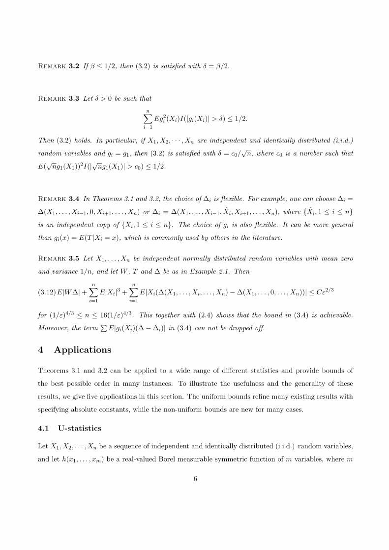
Remark 3.2 If β ≤ 1/2, then (3.2) is satisfied with δ = β/2.

Remark 3.3 Let δ > 0 be such that

n∑i=1

Eg2i (Xi)I(|gi(Xi)| > δ) ≤ 1/2.

Then (3.2) holds. In particular, if X1, X2, · · · , Xn are independent and identically distributed (i.i.d.)

random variables and gi = g1, then (3.2) is satisfied with δ = c0/√n, where c0 is a number such that

E(√ng1(X1))2I(|

√ng1(X1)| > c0) ≤ 1/2.

Remark 3.4 In Theorems 3.1 and 3.2, the choice of ∆i is flexible. For example, one can choose ∆i =

∆(X1, . . . , Xi−1, 0, Xi+1, . . . , Xn) or ∆i = ∆(X1, . . . , Xi−1, Xi, Xi+1, . . . , Xn), where {Xi, 1 ≤ i ≤ n}

is an independent copy of {Xi, 1 ≤ i ≤ n}. The choice of gi is also flexible. It can be more general

than gi(x) = E(T |Xi = x), which is commonly used by others in the literature.

Remark 3.5 Let X1, . . . , Xn be independent normally distributed random variables with mean zero

and variance 1/n, and let W , T and ∆ be as in Example 2.1. Then

E|W∆|+n∑

i=1

E|Xi|3 +n∑

i=1

E|Xi(∆(X1, . . . , Xi, . . . , Xn)−∆(X1, . . . , 0, . . . , Xn))| ≤ Cε2/3(3.12)

for (1/ε)4/3 ≤ n ≤ 16(1/ε)4/3. This together with (2.4) shows that the bound in (3.4) is achievable.

Moreover, the term∑E|gi(Xi)(∆−∆i)| in (3.4) can not be dropped off.

4 Applications

Theorems 3.1 and 3.2 can be applied to a wide range of different statistics and provide bounds of

the best possible order in many instances. To illustrate the usefulness and the generality of these

results, we give five applications in this section. The uniform bounds refine many existing results with

specifying absolute constants, while the non-uniform bounds are new for many cases.

4.1 U-statistics

Let X1, X2, . . . , Xn be a sequence of independent and identically distributed (i.i.d.) random variables,

and let h(x1, . . . , xm) be a real-valued Borel measurable symmetric function of m variables, where m

6

(2 ≤ m < n) may depend on n. Consider the Hoeffding (1948) U -statistic

Un =( nm

)−1 ∑1≤i1<...<im≤n

h(Xi1 , . . . , Xim).

The U-statistic elegantly and usefully generalizes the notion of a sample mean. Numerous investi-

gations on the limiting properties of the U-statistics have been done during the last few decades. A

systematic presentation of the theory of U-statistics was given in Koroljuk and Borovskikh (1994). We

refer the study on uniform Berry-Esseen bound for U-statistics to Filippova (1962), Grams and Serfling

(1973), Bickel (1974), Chan and Wierman (1977), Callaert and Janseen (1978), Serfling (1980),Van

Zwet (1984), and Friedrich (1989). One can also refer to Wang, Jing and Zhao (2000) on uniform

Berry-Esseen bound for studentized U-statistics.

Applying Theorems 3.1 and 3.2 to the U-statistic, we have

Theorem 4.1 Assume that Eh(X1, . . . , Xm) = 0 and σ2 = Eh2(X1, . . . , Xm) < ∞. Let g(x) =

E(h(X1, X2, . . . , Xm)|X1 = x) and σ21 = Eg2(X1). Assume that σ1 > 0. Then

supz|P( √

n

mσ1Un ≤ z

)− P

( 1√nσ1

n∑i=1

g(Xi) ≤ z)| ≤ (1 +

√2)(m− 1)σ

(m(n−m+ 1))1/2σ1+

c0√n,(4.1)

where c0 is a constant such that Eg2(X1)I(|g(X1)| > c0σ1) ≤ σ21/2. If in addition E|g(X1)|p <∞ for

2 < p ≤ 3, then

supz|P( √

n

mσ1Un ≤ z

)− Φ(z)| ≤ (1 +

√2)(m− 1)σ

(m(n−m+ 1))1/2σ1+

6.1E|g(X1)|p

n(p−2)/2σp1

(4.2)

and for z ∈ R1,

|P( √

n

mσ1Un ≤ z

)− Φ(z)| ≤ 9mσ2

(1 + |z|)2(n−m+ 1)σ21

+13.5e−|z|/3m1/2σ

(n−m+ 1)1/2σ1(4.3)

+CE|g(X1)|p

(1 + |z|)pn(p−2)/2σp1

.

Moreover, if E|h(X1, . . . , Xm)|p <∞ for 2 < p ≤ 3, then for z ∈ R1,

|P( √

n

mσ1Un ≤ z

)− Φ(z)|(4.4)

≤ Cm1/2E|h(X1, . . . , Xm)|p

(1 + |z|)p(n−m+ 1)1/2σp1

+CE|g(X1)|p

(1 + |z|)pn(p−2)/2σp1

.

7

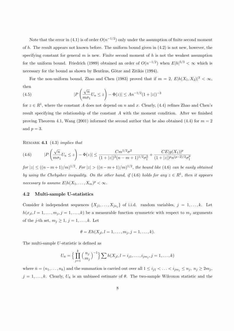
Note that the error in (4.1) is of order O(n−1/2) only under the assumption of finite second moment

of h. The result appears not known before. The uniform bound given in (4.2) is not new, however, the

specifying constant for general m is new. Finite second moment of h is not the weakest assumption

for the uniform bound. Friedrich (1989) obtained an order of O(n−1/2) when E|h|5/3 < ∞ which is

necessary for the bound as shown by Bentkus, Gotze and Zitikis (1994).

For the non-uniform bound, Zhao and Chen (1983) proved that if m = 2, E|h(X1, X2)|3 < ∞,

then

|P( √

n

mσ1Un ≤ z

)− Φ(z)| ≤ An−1/2(1 + |z|)−3(4.5)

for z ∈ R1, where the constant A does not depend on n and x. Clearly, (4.4) refines Zhao and Chen’s

result specifying the relationship of the constant A with the moment condition. After we finished

proving Theorem 4.1, Wang (2001) informed the second author that he also obtained (4.4) for m = 2

and p = 3.

Remark 4.1 (4.3) implies that

|P( √

n

mσ1Un ≤ z

)− Φ(z)| ≤ Cm1/2σ2

(1 + |z|)3(n−m+ 1)1/2σ21

+CE|g(X1)|p

(1 + |z|)pn(p−2)/2σp1

(4.6)

for |z| ≤ ((n−m+1)/m)1/2. For |z| > ((n−m+1)/m)1/2, the bound like (4.6) can be easily obtained

by using the Chebyshev inequality. On the other hand, if (4.6) holds for any z ∈ R1, then it appears

necessary to assume E|h(X1, . . . , Xm)p <∞.

4.2 Multi-sample U-statistics

Consider k independent sequences {Xj1, . . . , Xjnj} of i.i.d. random variables, j = 1, . . . , k. Let

h(xjl, l = 1, . . . ,mj , j = 1, . . . , k) be a measurable function symmetric with respect to mj arguments

of the j-th set, mj ≥ 1, j = 1, . . . , k. Let

θ = Eh(Xjl, l = 1, . . . ,mj , j = 1, . . . , k).

The multi-sample U -statistic is defined as

Un ={ k∏

j=1

( nj

mj

)−1}∑h(Xjl, l = ij1, . . . , ijmj , j = 1, . . . , k)

where n = (n1, . . . , nk) and the summation is carried out over all 1 ≤ ij1 < . . . < ijmj ≤ nj , nj ≥ 2mj ,

j = 1, . . . , k. Clearly, Un is an unbiased estimate of θ. The two-sample Wilcoxon statistic and the

8

two-sample ω2-statistic are two typical examples of the multi-sample U -statistics. Without loss of

generality, assume θ = 0. For j = 1, . . . , k, define

hj(x) = E(h(X11, . . . , X1m1 ; . . . ;Xk1, . . . , Xkmk

)|Xj1 = x)

and let σ2j = Eh2

j (Xj1) and

σ2n =

k∑j=1

m2j

njσ2

j .

A uniform Berry-Esseen bound with order O((min1≤j≤k nj)−1/2) for the multi-sample U-statistics was

obtained by Helmers and Janssen (1982) and Borovskich (1983) (see, [Koroljuk and Borovskich (1994),

pp. 304-311.]). Next theorem refines their results.

Theorem 4.2 Assume that θ = 0, σ2 := Eh2(X11, . . . , X1m1 ; . . . ;Xk1, . . . , Xkmk) <∞ and

max1≤j≤k σj > 0. Then for 2 < p ≤ 3

supz|P(σ−1

n Un ≤ z)− Φ(z)| ≤ (1 +

√2)σ

σn

k∑j=1

m2j

nj+

6.6σp

n

k∑j=1

mpj

np−1j

E|hj(Xj1)|p(4.7)

and for z ∈ R1

|P(σ−1

n Un ≤ z)− Φ(z)| ≤ 9σ2

(1 + |z|)2σ2n

( k∑j=1

m2j

nj

)2+ 13.5e−|z|/3 σ

σn

k∑j=1

m2j

nj(4.8)

+C

(1 + |z|)pσpn

k∑j=1

mpjE|hj(Xj1)|p

np−1j

.

4.3 L-statistics

Let X1, . . . , Xn be i.i.d. random variables with a common distribution function F , and let Fn be the

empirical distribution function defined by

Fn(x) = n−1n∑

i=1

I(Xi ≤ x) for x ∈ R1.

Let J(t) be a real-valued function on [0, 1] and define

T (G) =∫ ∞

−∞xJ(G(x))dG(x)

for non-decreasing measurable function G. Put

σ2 =∫ ∞

−∞

∫ ∞

−∞J(F (s))J(F (t))F (min(s, t))(1− F (max(s, t))dsdt

9

and

g(x) =∫ ∞

−∞(I(x ≤ s)− F (s))J(F (s))ds.

The statistic T (Fn) is called an L-statistic (see [Serfling (1980), Chapter 8]). Uniform Berry-Esseen

bounds for L-statistic for smoothing J were given by Helmers (1977), and Helmers, Janssen and

Serfling (1990). Applying Theorems 3.1 and 3.2 yields the following uniform and non-uniform bounds

for L-statistic.

Theorem 4.3 Let n ≥ 4. Assume that EX21 < ∞ and E|g(X1)|p < ∞ for 2 < p ≤ 3. If the weight

function J(t) is Lipschitz of order 1 on [0, 1], that is, there exists a constant c0 such that

|J(t)− J(s)| ≤ c0|t− s| for 0 ≤ s, t ≤ 1(4.9)

then

supz|P (

√nσ−1(T (Fn)− T (F )) ≤ z)− Φ(z)| ≤ (1 +

√2)c0||X1||2√nσ

+6.1E|g(X1)|p

n(p−2)/2σp(4.10)

and

|P (√nσ−1(T (Fn)− T (F )) ≤ z)− Φ(z)| ≤ 9c20EX

21

(1 + |z|)2nσ2+

C

(1 + |z|)p

(c0||X1||2√nσ

+E|g(X1)|p

n(p−2)/2σp

)(4.11)

4.4 Random sums of independent random variables with non-random centering

Let {Xi, i ≥ 1} be i.i.d. random variables with EXi = µ and Var(Xi) = σ2, and let {Nn, n ≥ 1}

be a sequence of non-negative integer-valued random variables that are independent of {Xi, i ≥ 1}.

Assume that EN2n <∞ and

Nn − ENn√Var(Nn)

d.−→ N(0, 1).

Then by Robbins (1948), ∑Nni=1Xi − (ENn)µ√

σ2ENn + µ2Var(Nn)d.−→ N(0, 1).

This is a special case of limit theorems for random sums with non-random centering. This kind

of problems arises in the study, for example, of Galton-Watson branching processes. We refer to

Finkelstein, Kruglov and Tucker (1994) and references therein for recent developments in this area.

As another application of our general result, we give a uniform Berry-Esseen bound for the random

sum.

10

Theorem 4.4 Let {Yi, i ≥ 1} be i.i.d. non-negative integer-valued random variables with EYi = ν

and Var(Yi) = τ2. Put Nn =∑n

i=1 Yi. Assume that E|Xi|3 <∞ and that {Yi, i ≥ 1} and {Xi, i ≥ 1}

are independent. Then

supx|P( ∑Nn

i=1Xi − nµν√n(νσ2 + τ2µ2)

≤ x)− Φ(x)| ≤ Cn−1/2

(τ2

ν2+E|X1|3

σ3+

σ

µ√ν

).(4.12)

4.5 Functions of non-linear statistics

Let X1, X2, . . . , Xn be a random sample and Θn = Θn(X1, . . . , Xn) be a weak consistent estimator of

an unknown parameter θ. Assume that Θn can be written as

Θn = θ +1√n

( n∑i=1

gi(Xi) + ∆)

where gi are Borel measurable functions with Egi(Xi) = 0 and∑n

i=1Eg2i (Xi) = 1, and ∆ :=

∆n(X1, . . . , Xn) → 0 in probability. Let h be a real-valued function differentiable in a neighborhood

of θ with g′(θ) 6= 0. Then, it is known that

√n(h(Θn)− h(θ))

h′(θ)d.−→ N(0, 1)

under some regularity conditions. When Θn is the sample mean, the Berry-Esseen bound and Edge-

worth expansion have been well studied (see Bhattacharya and Ghosh (1978)). The next theorem

shows that the results in Section 3 can be extended to functions of non-linear statistics.

Theorem 4.5 Assume that h′(θ) 6= 0 and δ(c0) = sup|x−θ|≤c0 |h′′(x)| <∞ for some c0 > 0. Then for

2 < p ≤ 3,

supz|P(√n(h(Θn)− h(θ))

h′(θ)≤ z

)− Φ(z)|(4.13)

≤(1 +

c0δ(c0)|h′(θ)|

)(E|W∆|+

n∑i=1

E|gi(Xi)(∆−∆i)|)

+6.1n∑

i=1

E|gi(Xi)|p +4c20n

+2E|∆|c0n1/2

+4.4c3−p

0 δ(c0)|h′(θ)|n(p−2)/2

,

where W =∑n

i=1 gi(Xi).

11

5 Proof of Main Theorems

Proof of Theorem 3.1. (3.5) follows from (3.4) and (1.4). When β > 1/2, (3.4) is trivial. For

β ≤ 1/2, (3.4) is a consequence of (3.3) and Remark 3.2. Thus, we only need to prove (3.3). Note that

−P (z − |∆| ≤W ≤ z) ≤ P (T ≤ z)− P (W ≤ z) ≤ P (z ≤W ≤ z + |∆|).(5.1)

It suffices to show that

P (z ≤W ≤ z + |∆|) ≤ 4δ + E|W∆|+n∑

i=1

E|gi(Xi)(∆−∆i)|(5.2)

and

P (z − |∆| ≤W ≤ z) ≤ 4δ + E|W∆|+n∑

i=1

E|gi(Xi)(∆−∆i)|(5.3)

where δ satisfies (3.2). Let

f∆(w) =

−|∆|/2− δ for w ≤ z − δ,

w − 12(2z + |∆|) for z − δ ≤ w ≤ z + |∆|+ δ,

|∆|/2 + δ for w > z + |∆|+ δ.

(5.4)

Let

ξi = gi(Xi), Mi(t) = ξi{I(−ξi ≤ t ≤ 0)− I(0 < t ≤ −ξi)},

Mi(t) = EMi(t), M(t) =n∑

i=1

Mi(t),M(t) = EM(t).

Since ξi and f∆i(W − ξi) are independent for 1 ≤ i ≤ n and Eξi = 0, we have

E{Wf∆(W )} =∑

1≤i≤n

E{ξi(f∆(W )− f∆(W − ξi))}(5.5)

+∑

1≤i≤n

E{ξi(f∆(W − ξi)− f∆i(W − ξi))}

:= H1 +H2.

Using the fact that M(t) ≥ 0 and f ′∆(w) ≥ 0, we have

H1 =∑

1≤i≤n

E{ξi

∫ 0

−ξi

f ′∆(W + t)dt}

(5.6)

=∑

1≤i≤n

E{∫ ∞

−∞f ′∆(W + t)Mi(t)dt

}= E

{∫ ∞

−∞f ′∆(W + t)M(t)dt

}12

≥ E{∫

|t|≤δf ′∆(W + t)M(t)dt

}≥ E

{I(z ≤W ≤ z + |∆|)

∫|t|≤δ

M(t)dt}

=∑

1≤i≤n

E{I(z ≤W ≤ z + |∆|)|ξi|min(δ, |ξi|)

}≥ H1,1 −H1,2,

where

H1,1 = P (z ≤W ≤ z + |∆|)∑

1≤i≤n

Eηi, H1,2 = E|∑

1≤i≤n

ηi − Eηi|, ηi = |ξi|min(δ, |ξi|).

By (3.2), ∑1≤i≤n

Eηi ≥ 1/2.

Hence

H1,1 ≥ (1/2)P (z ≤W ≤ z + |∆|).(5.7)

By the Cauchy-Schwarz inequality,

H1,2 ≤(E(

∑1≤i≤n

ηi − Eηi)2)1/2

(5.8)

≤( ∑

1≤i≤n

Eη2i

)1/2≤ δ.

As to H2, it is easy to see that

|f∆(w)− f∆i(w)| ≤∣∣∣|∆| − |∆i|

∣∣∣/2 ≤ |∆−∆i|/2.

Hence

|H2| ≤ (1/2)n∑

i=1

E|ξi(∆−∆i)|.(5.9)

Combining (5.5), (5.7), (5.8) and (5.9) yields

P (z ≤W ≤ z + |∆|) ≤ 2{E|Wf∆(W )|+ δ + (1/2)

n∑i=1

E|ξi(∆−∆i)|}

≤ E|W∆|+ 2δE|W |+ 2δ +n∑

i=1

E|ξi(∆−∆i)|

≤ 4δ + E|W∆|+n∑

i=1

E|ξi(∆−∆i)|.

13

This proves (5.2). Similarly, one can prove (5.3) and hence Theorem 3.1.

Proof of Theorem 3.2. First, we prove (3.9). For |z| ≤ 4, (3.9) holds by (3.5). For |z| > 4, consider

two cases.

Case 1.∑n

i=1E|gi(Xi)|p > 1/2.

By the Rosenthal (1970) inequality, we have

P (|W | > (|z| − 2)/3) ≤ P (|W | > |z|/6) ≤ (|z|/6)−pE|W |p(5.10)

≤ C(|z|+ 1)−p{( n∑

i=1

Eg2i (Xi)

)p/2+

n∑i=1

E|gi(Xi)|p}

≤ C(|z|+ 1)−pn∑

i=1

E|gi(Xi)|p.

Hence

|P (T ≤ z)− Φ(z)| ≤ P (|∆| > (|z|+ 1)/3) + P (|W | > (|z| − 2)/3) + P (|N(0, 1)| > |z|)

≤ P (|∆| > (|z|+ 1)/3) + C(|z|+ 1)−pn∑

i=1

E|gi(Xi)|p,

which shows that (3.9) holds.

Case 2.∑n

i=1E|gi(Xi)|p ≤ 1/2.

Similar to (5.10), we have

P (|W − gi(Xi)| > (|z| − 2)/3) ≤ C(|z|+ 1)−p{( n∑

j=1

Eg2j (Xj)

)p/2+

n∑j=1

E|gj(Xj)|p}≤ C(|z|+ 1)−p

and hence

γz ≤ P (|∆| > (|z|+ 1)/3) +n∑

i=1

((|z|+ 1)/3)−pE|gi(Xi)|p +n∑

i=1

C(|z|+ 1)−pE|gi(Xi)|p

≤ P (|∆| > (|z|+ 1)/3) + C(|z|+ 1)−pn∑

i=1

E|gi(Xi)|p.

By Remark 3.1, we can choose

δ =(2(p− 2)p−2

(p− 1)p−1

n∑i=1

E|gi(Xi)|p)1/(p−2)

≤ 2(p− 2)p−2

(p− 1)p−1

n∑i=1

E|gi(Xi)|p.

Combining the above inequalities with (3.6) and the non-uniform Berry-Essee bound for independent

random variables yields (3.9).

14

Next we prove (3.6). The main idea of the proof is first to truncate gi(Xi) and then adopt the

proof of Theorem 3.1 to the truncated sum. Without loss of generality, assume z ≥ 0 as we can simply

apply the result to −T . By (5.1), it suffices to show that

P (z − |∆| ≤W ≤ z) ≤ γz + e−z/3τ(5.11)

and

P (z ≤W ≤ z + |∆|) ≤ γz + e−z/3τ.(5.12)

Since the proof of (5.12) is similar to that of (5.11), we only prove (5.11). It is easy to see that

P (z − |∆| ≤W ≤ z) ≤ P (|∆| > (z + 1)/3) + P (z − |∆| ≤W ≤ z, |∆| ≤ (z + 1)/3).

Now (5.11) follows directly by Lemmas 5.1 and 5.2 below. This completes the proof of Theorem 3.2.

Lemma 5.1 Let

ξi = gi(Xi), ξi = ξiI(ξi ≤ 1), W =n∑

i=1

ξi.

Then

P (z − |∆| ≤W ≤ z, |∆| ≤ (z + 1)/3)(5.13)

≤ P (z − |∆| ≤ W ≤ z, |∆| ≤ (z + 1)/3)

+n∑

i=1

P (ξi > (z + 1)/3) +n∑

i=1

P (W − ξi > (z − 2)/3)P (|ξi| > 1).

Proof. We have

P (z − |∆| ≤W ≤ z, |∆| ≤ (z + 1)/3)

≤ P (z − |∆| ≤W ≤ z, |∆| ≤ (z + 1)/3, max1≤i≤n

|ξi| ≤ 1)

+P (z − |∆| ≤W ≤ z, |∆| ≤ (z + 1)/3, max1≤i≤n

|ξi| > 1)

≤ P (z − |∆| ≤ W ≤ z, |∆| ≤ (z + 1)/3) +n∑

i=1

P (W > (2z − 1)/3, |ξi| > 1)

and

n∑i=1

P (W > (2z − 1)/3, |ξi| > 1)

15

≤n∑

i=1

P (ξi > (z + 1)/3) +n∑

i=1

P (W > (2z − 1)/3, ξi ≤ (z + 1)/3, |ξi| > 1)

≤n∑

i=1

P (ξi > (z + 1)/3) +n∑

i=1

P (W − ξi > (z − 2)/3, |ξi| > 1)

=n∑

i=1

P (ξi > (z + 1)/3) +n∑

i=1

P (W − ξi > (z − 2)/3)P (|ξi| > 1),

as desired.

Lemma 5.2 We have

P (z − |∆| ≤ W ≤ z, |∆| ≤ (z + 1)/3) ≤ e−z/3τ.(5.14)

Proof. Noting that Eξi ≤ 0, es ≤ 1 + s+ s2(ea − 1− a)a−2 for s ≤ a and a > 0 and that aξi ≤ a,

we have for a > 0

EeaW =n∏

i=1

Eeaξi(5.15)

≤n∏

i=1

(1 + aEξi + (ea − 1− a)Eξ2i

)≤ exp

((ea − 1− a)

n∑i=1

Eξ2i

)≤ exp

((ea − 1− a)

n∑i=1

Eξ2i

)= exp(ea − 1− a).

In particular, we have EeW/2 ≤ exp(e1/2 − 1.5). If δ ≥ 0.07, then

P (z − |∆| ≤ W ≤ z, |∆| ≤ (z + 1)/3)

≤ P (W > (2z − 1)/3) ≤ e−z/3+1/6EeW/2

≤ e−z/3 exp(e.5 − 4/3) ≤ 1.38e−z/3 ≤ 20δ e−z/3.

This proves (5.14) when δ ≥ 0.07.

For δ < 0.07, let

f∆(w) =

0 for w ≤ z − |∆| − δ,

ew/2(w − z + |∆|+ δ) for z − |∆| − δ ≤ w ≤ z + δ,

ew/2(|∆|+ 2δ) for w > z + δ.

(5.16)

Put

Mi(t) = ξi{I(−ξi ≤ t ≤ 0)− I(0 < t ≤ −ξi)}, M(t) =n∑

i=1

Mi(t).

16

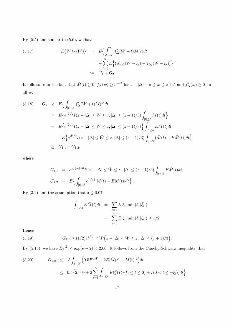
By (5.5) and similar to (5.6), we have

E{Wf∆(W )} = E{∫ ∞

−∞f ′∆(W + t)M(t)dt(5.17)

+n∑

i=1

E{ξi(f∆(W − ξi)− f∆i(W − ξi))

}:= G1 +G2,

It follows from the fact that M(t) ≥ 0, f ′∆(w) ≥ ew/2 for z − |∆| − δ ≤ w ≤ z + δ and f ′∆(w) ≥ 0 for

all w,

G1 ≥ E{∫

|t|≤δf ′∆(W + t)M(t)dt(5.18)

≥ E{eW/2I(z − |∆| ≤ W ≤ z, |∆| ≤ (z + 1)/3)

∫|t|≤δ

M(t)dt}

= E{eW/2I(z − |∆| ≤ W ≤ z, |∆| ≤ (z + 1)/3)

}∫|t|≤δ

EM(t)dt

+E{eW/2I(z − |∆| ≤ W ≤ z, |∆| ≤ (z + 1)/3)

∫|t|≤δ

(M(t)− EM(t))dt}

≥ G1,1 −G1,2,

where

G1,1 = ez/3−1/6P (z − |∆| ≤ W ≤ z, |∆| ≤ (z + 1)/3)∫|t|≤δ

EM(t)dt,

G1,2 = E{∫

|t|≤δeW/2|M(t)− EM(t)|dt

}.

By (3.2) and the assumption that δ ≤ 0.07,∫|t|≤δ

EM(t)dt =n∑

i=1

E|ξi|min(δ, |ξi|)

=n∑

i=1

E|ξi|min(δ, |ξi|) ≥ 1/2.

Hence

G1,1 ≥ (1/2)ez/3−1/6P(z − |∆| ≤ W ≤ z, |∆| ≤ (z + 1)/3

).(5.19)

By (5.15), we have EeW ≤ exp(e− 2) < 2.06. It follows from the Cauchy-Schwarz inequality that

G1,2 ≤ .5∫|t|≤δ

(0.5EeW + 2E|M(t)−M(t)|2

)dt(5.20)

≤ 0.5{2.06δ + 2

n∑i=1

∫|t|≤δ

Eξ2i (I(−ξi ≤ t ≤ 0) + I(0 < t ≤ −ξi))dt}

17

= 0.5{2.06δ + 2

n∑i=1

Eξ2i min(δ, |ξi|)}

≤ 0.5{2.06δ + 2δ

n∑i=1

Eξ2i

}≤ 2.03δ.

As to G2, it is easy to see that

|f∆(w)− f∆i(w)| ≤ ew/2∣∣∣|∆| − |∆i|

∣∣∣ ≤ ew/2|∆−∆i|.

Hence, by the Holder inequality, (5.15) and the assumption that ξi and W − ξi are independent

|G2| ≤n∑

i=1

E|ξie(W−ξi)/2(∆−∆i)|(5.21)

≤n∑

i=1

(Eξ2i e

W−ξi

)1/2(E(∆−∆i)2

)1/2

=n∑

i=1

(Eξ2iEe

W−ξi

)1/2||∆−∆i||2

≤ 1.44n∑

i=1

||ξi||2 ||∆−∆i||2.

Following the proof of (5.15) and by using |es − 1| ≤ |s|(ea − 1)/a for s ≤ a and a > 0, we have

EW 2eW =n∑

i=1

Eξ2i eξiEeW−ξi +

∑1≤i6=j≤n

Eξi(eξi − 1)Eξj(eξj − 1)EeW−ξi−ξj

≤ 2.06 en∑

i=1

Eξ2i + 2.06(e− 1)2∑

1≤i6=j≤n

Eξ2iEξ2j

≤ 2.06 e+ 2.06(e− 1)2 < 3.422.

Thus, we obtain

E{Wf∆(W )} ≤ E|W |eW/2(|∆|+ 2δ)(5.22)

≤{||∆||2 + 2δ

}(E(W 2eW )

)1/2

≤ 3.42(||∆||2 + 2δ).

Combining (5.17), (5.19), (5.20), (5.21) and (5.22) yields

P (z − |∆| ≤ W ≤ z, |∆| ≤ (z + 1)/3)

≤ 2e−z/3+1/6{3.42(||∆||2 + 2δ) + 2.03δ + 1.44

n∑i=1

||ξi||2 ||∆−∆i||2}

≤ e−z/3{21δ + 8.1||∆||2 + 3.5

n∑i=1

||ξi||2 ||∆−∆i||2}

= e−z/3τ.

18

This proves (5.14).

Proof of Remark 3.1. It is known that for x ≥ 0, y ≥ 0, α > 0, γ > 0 with α+ γ = 1

xαyγ ≤ αx+ γy,

which yields with α = (p−2)/(p−1), γ = 1/(p−1), x = b(p−1)/(p−2) and y =((p−2

p−1)p−2 ap−1

bp−2

)1/(p−1),

a = xαyγ ≤ αx+ γy = b+(p− 2)p−2

(p− 1)p−1

ap−1

bp−2

or

b ≥ a− (p− 2)p−2

(p− 1)p−1

ap−1

bp−2.

On the other hand, it is clear that

a ≥ a− (p− 2)p−2

(p− 1)p−1

ap−1

bp−2.

This proves (3.11). Now (3.2) follows directly from (3.11), (3.10) and the assumption (1.1).

Proof of Remark 3.2. Note that δ = β/2 ≤ 1/4. Applying (3.11) with p = 3 yieldsn∑

i=1

E|gi(Xi)|min(δ, |gi(Xi)|)

≥n∑

i=1

E|gi(Xi)|I(|gi(Xi)| ≤ 1) min(δ, |gi(Xi)|)

≥n∑

i=1

{Eg2

i (Xi)I(|gi(Xi)| ≤ 1)− E|gi(Xi)|3I(|gi(Xi)| ≤ 1)/(4δ)}

= 1−(4δ

n∑i=1

Eg2i (Xi)I(|gi(Xi)| > 1) +

n∑i=1

E|gi(Xi)|3I(|gi(Xi)| ≤ 1))/(4δ)

≥ 1− β/(4δ) = 1/2.

This proves Remark 3.2.

Proof of Remark 3.5. The proof is postponed to the end of next section.

6 Proofs of Other Theorems

6.1 Proof of Theorem 4.1

For 1 ≤ k ≤ m, let hk(x1, . . . , xk) = E(h(X1, . . . , Xm)|X1 = x1, . . . , Xk = xk) and hk(x1, . . . , xk) =

hk(x1, . . . , xk)−∑k

i=1 g(xi). Observing that

Un = n−1mn∑

i=1

g(Xi) +( nm

)−1 ∑1≤i1<...<im≤n

hm(Xi1 , . . . , Xim),

19

we have √n

mσ1Un = W + ∆,

where

W =1√nσ1

n∑i=1

g(Xi),

∆ =√n

mσ1

( nm

)−1 ∑1≤i1<...<im

hm(Xi1 , . . . , Xim).

Let

∆l =√n

mσ1

( nm

)−1 ∑1≤i1<...<im,ij 6=l for all j

hm(Xi1 , . . . , Xim).

By Theorems 3.1 and 3.2 (with Remark 3.3 for proof of (4.1)), it suffices to show that

E∆2 ≤ (m− 1)2σ2

m(n−m+ 1)σ21

(6.1)

and

E|∆−∆l|2 ≤2(m− 1)2σ2

nm(n−m+ 1)σ21

.(6.2)

It is known that (see, e.g., [18], p.271)

E( ∑

1≤i1<...<im≤n

hm(Xi1 , . . . , Xim))2

(6.3)

=( nm

) m∑j=2

(mj

)( n−mm− j

)Eh2

j (X1, . . . , Xj).

Note that

Eh2j (X1, . . . , Xj)(6.4)

= Eh2j (X1, . . . , Xj)− 2

j∑i=1

E[g(Xi)hk(X1, . . . , Xj)] + E(j∑

i=1

g(Xi))2

= Eh2j (X1, . . . , Xj)− 2jE[g(X1)E(h(X1, . . . , Xm)|X1, . . . , Xj)] + kEg2(X1)

= Eh2j (X1, . . . , Xj)− 2jE[g(X1)h(X1, . . . , Xm)] + jEg2(X1)

= Eh2j (X1, . . . , Xj)− 2jEg2(X1) + jEg2(X1)

= Eh2j (X1, . . . , Xj)− jEg2

1(X1).

We next prove that for 2 ≤ j ≤ m

Eh2j−1(X1 . . . , Xj−1) ≤

j − 1j

Eh2j (X1, . . . , Xj)(6.5)

20

Since Eh22(X1, X2) ≥ 0, (6.5) holds for j = 2 by (6.4). Assume that (6.5) is true for j. Then

E(hj+1(X1, . . . , Xj+1)− hj(X1, . . . , Xj)− hj(X2, . . . , Xj+1))2(6.6)

= Eh2j+1(X1, . . . , Xj+1)− 4E[hj+1(X1, . . . , Xj+1)hj(X1, . . . , Xj)]

+2Eh2j (X1, . . . , Xj) + 2Ehj(X1, . . . , Xj)hj(X2, . . . , Xj+1)

= Eh2j+1(X1, . . . , Xj+1)− 2Eh2

j (X1, . . . , Xj)

+2E(E(hj(X1, . . . , Xj)hj(X2, . . . , Xj+1) | X2, . . . , Xj)

)= Eh2

j+1(X1, . . . , Xj+1)− 2Eh2j (X1, . . . , Xj) + 2Eh2

j−1(X1, . . . , Xj−1).

On the other hand, we have

E(hj+1(X1, . . . , Xj+1)− hj(X1, . . . , Xj)− hj(X2, . . . , Xj+1))2(6.7)

≥ E(E(hj+1(X1, . . . , Xj+1)− hj(X1, . . . , Xj)− hj(X2, . . . , Xj+1) | X1, . . . , Xj)

)2

= Eh2j−1(X1, . . . , Xj−1).

Combining (6.5) and (6.6) yields

2Eh2j (X1, . . . , Xj) ≤ Eh2

j+1(X1, . . . , Xj+1) + Eh2j−1(X1, . . . , Xj−1)

≤ Eh2j+1(X1, . . . , Xj+1) +

j − 1j

Eh2j (X1, . . . , Xj)

by the induction hypothesis, which in turn reduces to (6.4) for j + 1. This proves (6.4).

It follows from (6.4) that

Eh2j (X1, . . . , Xj) ≤

j

mEh2

m(X1, . . . , Xm) =j

mσ2.(6.8)

To complete the proof of (6.1), we need the following two inequalities:

m∑j=2

(mj

)( n−mm− j

) jm≤ m(m− 1)2

(n−m+ 1)n

( nm

)(6.9)

andm−1∑j=1

(m− 1j

)( n−mm− 1− j

)j + 1m

≤ 2(m− 1)2

(n−m+ 1)n

( nm

)(6.10)

for n > m ≥ 2. In fact, we have

m∑j=2

(mj

)( n−mm− j

) jm

21

=m∑

j=2

(m− 1j − 1

)( n−mm− j

)

=m−1∑j=1

(m− 1j

)( n−mm− 1− j

)=

( n− 1m− 1

)−( n−mm− 1

)=

( n− 1m− 1

){1− (n−m)!/(n−m−m+ 1)!

(n− 1)!/(n−m)!

}=

( n− 1m− 1

){1−

n−1∏j=n−m+1

(1− m− 1j

)}

≤( n− 1m− 1

) n−1∑j=n−m+1

m− 1j

≤( n− 1m− 1

) (m− 1)2

n−m+ 1

=(m− 1)2m

(n−m+ 1)n

( nm

)and

m−1∑j=1

(m− 1j

)( n−mm− 1− j

)j + 1m

=m− 1m

m−1∑j=1

(m− 1j

)( n−mm− 1− j

) j

m− 1+

1m

m−1∑j=1

(m− 1j

)( n−mm− 1− j

)

=m− 1m

m−2∑j=0

(m− 2j

)( n−mm− 2− j

)+

1m

m−1∑j=1

(m− 1j

)( n−mm− 1− j

)=

m− 1m

( n− 2m− 2

)+

1m{( n− 1m− 1

)−( n−mm− 1

)}

≤( n− 1m− 1

)( (m− 1)2

m(n− 1)+

(m− 1)2

(n−m+ 1)m

)≤ 2(m− 1)2

(n−m+ 1)n

( nm

).

From (6.8) and (6.9) we obtain that

E∆2 =n

m2σ21

( nm

)−2E{ ∑

1≤i1<...<im≤n

hm(X1, . . . , Xm)}2

(6.11)

≤ n

m2σ21

( nm

)−1m∑

j=2

(mj

)( n−mm− j

)Eh2

j (X1, . . . , Xj)

≤ nσ2

m2σ21

( nm

)−1m∑

j=2

(mj

)( n−mm− j

) jm

22

≤ (m− 1)2σ2

(n−m+ 1)mσ21

.

This proves (6.1).

Similarly, by (6.10)

E(∆−∆l)2 =n

m2σ21

( nm

)−2E({ ∑

1≤i1<...<im≤n

−∑

1≤i1<...<im≤n, all ij 6=l

}hm(Xi1 , . . . , Xim)

)2(6.12)

=n

m2σ21

( nm

)−2E( ∑

1≤i1<...<im−1≤n−1

hm(Xi1 , . . . , Xim−1 , Xm))2

=n

m2σ21

( nm

)−2( n− 1m− 1

)m−1∑j=1

(m− 1j

)( n−mm− 1− j

)Eh2

j+1(X1, . . . , Xj)

≤ n

m2σ21

( nm

)−2( n− 1m− 1

)m−1∑j=1

(m− 1j

)( n−mm− 1− j

)Eh2

j+1(X1, . . . , Xj)

≤ σ2

mσ21

( nm

)−1m−1∑j=1

(m− 1j

)( n−mm− 1− j

)j + 1m

≤ 2(m− 1)2 σ2

mn(n−m+ 1)σ21

.

This proves (6.2) and hence completes the proof of Theorem 4.1.

6.2 Proof of Theorem 4.2

We follow a similar argument as that in the proof of Theorem 4.1. For 1 ≤ j ≤ k, let Xj =

(Xj1, . . . , Xjmj ) and xj = (xj1, . . . , xjmj ) and define

h(x1, . . . ,xk) = h(x1, . . . ,xk)−k∑

j=1

mj∑i=1

hj(xji).

For the given U -statistic Un, we define its projection

Un =k∑

j=1

nj∑l=1

E(Un|Xjl).

Since

mj/nj =( nj − 1mj − 1

)/( nj

mj

),

we have

Un =k∑

j=1

nj∑l=1

mj

njhj(Xjl).

23

The difference Un − Un can be rewritten as

Un − Un ={ k∏

j=1

( nj

mj

)−1}∑h(X1i1

, . . . ,Xkik),

where Xjij= (Xjij1 , . . . , Xjijmj

) and the summation is carried out over all indices 1 ≤ ij1 < ij2 <

. . . < ijmj ≤ nj , j = 1, 2, . . . , k. Thus, we have

σ−1n Un = W + ∆

with

W = σ−1n

k∑j=1

nj∑l=1

mj

njhj(Xjl),

∆ = σ−1n

{ k∏j=1

( nj

mj

)−1}∑h(X1i1

, . . . ,Xkik).

Let

∆jl = σ−1n

{ k∏v=1

( nv

mv

)−1}∑(jl)h(X1i1

, . . . ,Xkik),

where the summation is carried out over all indices 1 ≤ iv1 < iv2 < . . . < ivmv ≤ nv, 1 ≤ v ≤ k, v 6= j

and 1 ≤ ij1 < ij2 < . . . < ijmj ≤ nj with ijs 6= l for 1 ≤ s ≤ mj .

By Theorems 3.1 and 3.2, it suffices to show that

E∆2 ≤ σ2

σ2n

( k∑j=1

m2j

nj

)2(6.13)

and

E|∆−∆jl|2 ≤2σ2m2

j

n2j σ

2n

k∑v=1

m2v

nv(6.14)

For 0 ≤ dj ≤ mj , 1 ≤ j ≤ k let

Yd1,...,dk(xji, 1 ≤ i ≤ dj , 1 ≤ j ≤ k) = Eh(xj1, . . . , xjd1 , Xjdj+1, . . . , Xjmj , 1 ≤ j ≤ k)

and

yd1,...,dk= EY 2

d1,...,dk(Xji, 1 ≤ i ≤ dj , 1 ≤ j ≤ k).

Noting that

E(h(X1i1, . . . ,Xkik

)|Xjl) = 0 for every 1 ≤ l ≤ mj , 1 ≤ j ≤ k,

24

we have (see (4.5.8) in [18])

E(Un − Un

)2(6.15)

={ k∏

j=1

( nj

mj

)−1} ∑d1 + . . . + dk ≥ 2

0 ≤ dj ≤ mj , 1 ≤ j ≤ k

k∏j=1

{(mj

dj

)( nj −mj

mj − dj

)}yd1,...,dk

≤ σ2{ k∏

j=1

( nj

mj

)−1} ∑d1 + . . . + dk ≥ 2

0 ≤ dj ≤ mj , 1 ≤ j ≤ k

k∏j=1

{(mj

dj

)( nj −mj

mj − dj

)}

≤ σ2( k∑

j=1

m2j

nj

)2,

where in the last inequality we used the fact that

∑d1 + . . . + dk ≥ 2

0 ≤ dj ≤ mj , 1 ≤ j ≤ k

k∏j=1

{(mj

dj

)( nj −mj

mj − dj

)}≤( k∑

j=1

m2j

nj

)2k∏

j=1

( nj

mj

).(6.16)

(See below for proof). This proves (6.13).

As to (6.14), consider j = 1 only. Similar to (6.12) and (6.15), we have (with X∗1i1

=

(X1i1,1 , . . . , X1i1,m1−1 , X1,m1))

σ2nE|∆−∆1l|2

={ k∏

v=1

( nv

mv

)}−2E( ∑

1 ≤ iv1 < iv2 < . . . < ivmv ≤ nv, 2 ≤ v ≤ k1 ≤ i1,1 < i1,2 < . . . < i1,mj−1 ≤ nj − 1

h(X∗1i1,X2i2

, . . . ,Xkik))2

≤ σ2{ k∏

v=1

( nv

mv

)}−2( n1 − 1m1 − 1

) k∏v=2

( nv

mv

)∑

d1 + . . . + dk ≥ 10 ≤ d1 ≤ m1 − 1, 0 ≤ dv ≤ mv, 2 ≤ v ≤ k

(m1 − 1d1

)( n1 −m1

m1 − 1− d1

) k∏v=2

(mv

dv

)( nv −mv

mv − dv

)

≤ σ2m1

n1

{ k∏v=1

( nv

mv

)}−1{ ∑1≤d1≤m1−1

+∑

2≤v≤k

∑d1=0,1≤dv≤mv

}

≤ σ2m1

n1

{ k∏v=1

( nv

mv

)}−1{ (m1 − 1)2

n1 −m1 + 1

( n1 − 1m1 − 1

) k∏j=2

( nj

mj

)

+( n1 −m1

m1 − 1

) ∑2≤v≤k

m2v

nv −mv + 1

k∏j=2

( nj

mj

)}

25

≤ σ2m21

n21

∑1≤v≤k

m2v

nv −mv + 1≤ 2σ2m2

1

n21

∑1≤v≤k

m2v

nv

for n1 ≥ 2m1. This proves (6.14).

Now we prove (6.16). Consider two cases in the summation:

Case 1: At least one of dj ≥ 2, say d1 ≥ 2. In this case, by (6.9)

∑d1 ≥ 2

1 ≤ dj ≤ mj , 1 ≤ j ≤ k

k∏j=1

{(mj

dj

)( nj −mj

mj − dj

)}

≤{ k∏

j=2

( nj

mj

)} ∑2≤d1≤m1

(m1

d1

)( n1 −m1

m1 − d1

)

≤{ k∏

j=2

( nj

mj

)}m2

∑2≤d1≤m1

(m1

d1

)( n1 −m1

m1 − d1

)d1

m

≤ m21(m1 − 1)2

2n1(n1 −m1 + 1)

k∏j=1

( nj

mj

)

≤ m41

n21

k∏j=1

( nj

mj

)for n1 ≥ 2m1.

Case 2. At least two of {dj} are equal to 1, say d1 = d2 = 1. Then

∑d1=d2=1

k∏j=1

{(mj

dj

)( nj −mj

mj − dj

)}

= m1m2

( n1 −m1

m1 − 1

)( n2 −m2

m2 − 1

) k∏j=3

( nj

mj

)

≤ m21m

22

n1 n2

k∏j=1

( nj

mj

).

Thus, we have ∑d1 + . . . + dk ≥ 2

1 ≤ dj ≤ mj , 1 ≤ j ≤ k

k∏j=1

{(mj

dj

)( nj −mj

mj − dj

)}

≤( k∑

j=1

m4j

n2j

+∑

1≤i6=j≤k

m2i m

2j

ni nj

) k∏j=1

( nj

mj

)

=( k∑

j=1

m2j

nj

)2k∏

j=1

( nj

mj

).

This proves (6.16). Now the proof of Theorem 4.2 is complete.

26

6.3 Proof of Theorem 4.3

Let ψ(t) =∫ t0 J(s)ds. As in [Serfling (1980), p.265], we have

T (Fn)− T (F ) = −∫ ∞

−∞[ψ(Fn(x))− ψ(F (x))]dx

and hence√nσ−1(T (Fn)− T (F )) = W + ∆,

where

W = − 1√nσ

n∑i=1

∫ ∞

−∞(I(Xi ≤ x)− F (x))J(F (x))dx

∆ = −√nσ−1

∫ ∞

−∞[ψ(Fn(x))− ψ(F (x))− (Fn(x)− F (x))J(F (x))]dx.

Let

ηi(x) = I(Xi ≤ x)− F (x),

gi(Xi) = − 1√nσ

∫ ∞

−∞(I(Xi ≤ x)− F (x))J(F (x))dx,

∆i = −√nσ−1

∫ ∞

−∞[ψ(Fn,i(x))− ψ(F (x))− (Fn,i(x)− F (x))J(F (x))]dx,

where Fn,i(x) =1n

{F (x) +

∑1≤j≤n,j 6=i

I(Xj ≤ x)}. We only need to prove

σ2E∆2 ≤ c20 n−1EX2

1(6.17)

and

σ2E|∆−∆i|2 ≤ 2c20n−2EX2

1(6.18)

Observe that the Lipschitz condition (4.9) implies

|ψ(t)− ψ(s)− (t− s)J(s)| = |∫ t−s

0(J(u+ s)− J(s))du| ≤ 0.5 c0(t− s)2(6.19)

for 0 ≤ s, t ≤ 1. Hence

σ2E∆2 ≤ 0.25c20 nE( ∫ ∞

−∞(Fn(x)− F (x))2dx

)2

= 0.25c20 n−3∫ ∞

−∞

∫ ∞

−∞E( n∑

i=1

n∑j=1

ηi(x)ηj(y))2dxdy

≤ 0.25c20 n−3∫ ∞

−∞

∫ ∞

−∞

(3n2Eη2

1(x)Eη21(y) + nE{η2

1(x)η21(y)}

)dxdy.

27

Observe that∫ ∞

−∞

∫ ∞

−∞Eη2

1(x)Eη21(y)dxdy =

( ∫ ∞

−∞F (x)(1− F (x))dx

)2≤ (E|X1|)2 ≤ EX2

1

and ∫ ∞

−∞

∫ ∞

−∞E{η2

1(x)η21(y)}dxdy

= 2∫ ∫

x≤yE{η2

1(x)η21(y)}dxdy

= 2∫ ∫

x≤y

{(1− F (x))2(1− F (y))2F (x)

+F 2(x)(1− F (y))2(F (y)− F (x)) + F 2(x)F 2(y)(1− F (y))}dxdy

≤ 2∫ ∫

x≤yF (x)(1− F (y))dxdy

= 2{∫ ∫

x≤y≤0+∫ ∫

0<x≤y+∫ ∫

x≤0,y>0

}F (x)(1− F (y))dxdy

≤ 2{∫

x≤0|x|F (x)dx+

∫y≥0

y(1− F (y))dy +∫

x≤0F (x)dx

∫y>0

(1− F (y))dy}

≤ 2{E(X−

1 )2 + E(X+1 )2 + EX−

1 EX+1

}≤ 4EX2

1

This proves (6.17).

Next we prove (6.18). Observe that

σ√n|∆−∆i| = |

∫ ∞

−∞[ψ(Fn(x))− ψ(Fn,i(x))− (Fn(x)− Fn,i(x))J(Fn,i(x))dx

+∫ ∞

−∞(Fn(x)− Fn,i(x))[J(Fn,i(x)− J(F (x))]dx|

≤ 0.5c0∫ ∞

−∞(Fn(x)− Fn,i(x))2dx

+c0∫ ∞

−∞|Fn(x)− Fn,i(x)||Fn,i(x)− F (x)|dx

≤ 0.5c0 n−2∫ ∞

−∞(I(Xi ≤ x)− F (x))2dx

+c0 n−2∫ ∞

−∞|I(Xi ≤ x)− F (x)| |

∑j 6=i

{I(Xj ≤ x)− F (x)}dx

= 0.5c0 n−2∫ ∞

−∞η2

i (x)dx+ c0 n−2∫ ∞

−∞|ηi(x)| |

∑j 6=i

ηj(x)|dx,

E( ∫ ∞

−∞η2

i (x)dx)2

=∫ ∞

−∞

∫ ∞

−∞Eη2

1(x)η21(y)dxdy ≤ 4EX2

1

28

and

E( ∫ ∞

−∞|ηi(x)| |

∑j 6=i

ηj(x)|dx)2

=∫ ∞

−∞

∫ ∞

−∞E{|ηi(x)| |

∑j 6=i

ηj(x)||ηi(y)| |∑j 6=i

ηj(y)|}dxdy

=∫ ∞

−∞

∫ ∞

−∞E|ηi(x)ηi(y)|E{|

∑j 6=i

ηj(x)||∑j 6=i

ηj(y)|}dxdy

≤∫ ∞

−∞

∫ ∞

−∞||ηi(x)||2||ηi(y)||2||

∑j 6=i

ηj(x)||2 ||∑j 6=i

ηj(y)||2dxdy

= (n− 1)∫ ∞

−∞

∫ ∞

−∞||ηi(x)||22||ηi(y)||22dxdy

≤ (n− 1)(E|X1|)2 ≤ (n− 1)EX21 .

Therefore

σ2E|∆−∆i|2 ≤ n−3c20E(0.5∫ ∞

−∞η2

i (x)dx+∫ ∞

−∞|ηi(x)| |

∑j 6=i

ηj(x)|dx)2

≤ n−3c20

{0.75E

( ∫ ∞

−∞η2

i (x)dx)2

+ 1.5E( ∫ ∞

−∞|ηi(x)| |

∑j 6=i

ηj(x)|dx)2}

≤ n−3c20

{3EX2

1 + 1.5(n− 1)EX21

}≤ 2n−2EX2

1 .

This proves (6.18) and hence the theorem.

6.4 Proof of Theorem 4.4

Let Z1 and Z2 be independent standard normal random variables that are independent of {Xi} and

{Yi}. Put

b =√νσ2 + τ2µ2, Tn =

∑Nni=1Xi − nµν√

nb, Hn =

∑Nni=1Xi −Nnµ√

Nnσ

and write

Tn =√Nnσ√nb

Hn +(Nn − nν)µ√

nb, Tn(Z1) =

√Nnσ√nb

Z1 +(Nn − nν)µ√

nb.

Applying the Berry-Esseen bound to Hn for given Nn yields

supx|P (Tn ≤ x)− P (Tn(Z1) ≤ x)|(6.20)

≤ P (|Nn − nν| > nν/2) + CE( |X1|3√

Nnσ3I{|Nn − nν| ≤ nν/2}

)≤ 4n−1ν−2τ2 + Cn−1/2ν−1/2σ−3E|X1|3.

29

Let

x∗ =

.5nν for x < .5nνx for .5nν ≤ x ≤ 1.5nν1.5nν for x > 1.5nν

Wn =Nn − nν√

nτ,

Tn(Z1) :=√N∗

nσ√nb

Z1 +(Nn − nν)µ√

nb

=τµ

b

(Wn +

σ√ν

τµZ1 + ∆

),

where

∆ =(√N∗

n −√nν)σZ1√

nτµ.

Let

∆i =(√

(Nn − Yi + ν)∗ −√nν)σZ1√

nτµ.

Then

E(|Wn∆| | Z1) ≤ |Z1|σ√nτµ

E( |Wn(Nn − nν)|√

nν=

|Z1|σ√nµ√ν

and

1√nτE(|(Yi − ν)(∆−∆i)| | Z1) ≤ |Z1|

n3/2τ2µ√νE(Yi − ν)2 =

|Z1|σn3/2µ

√ν.

Now letting

Tn(Z1, Z2) =τµ

b

(Z2 +

σ√ν

τµZ1

)and applying Theorem 3.1 for given Z1 yields

supx|P (Tn(Z1) ≤ x)− P (Tn(Z1, Z2) ≤ x)|(6.21)

≤ P (|Nn − nν| > 0.5nν) + supx|P (Tn(Z1) ≤ x)− P (Tn(Z1, Z2) ≤ x)|

≤ 4τ2

nν2+ C

(E|X1|3

n1/2σ3+

E|Z1|σn1/2µ

√ν

)≤ Cn−1/2

(τ2

ν2+E|X1|3

σ3+

σ

µ√ν

)It is clear that Tn(Z1, Z2) has a standard normal distribution. This proves (4.12) by (6.20) and (6.21).

30

6.5 Proof of Theorem 4.5

Since (4.13) is trivial if∑n

i=1E|gi(Xi)|p > 1/6, we assumen∑

i=1

E|gi(Xi)|p ≤ 1/6.(6.22)

Let W =∑n

i=1 gi(Xi). It is known that for 2 < p ≤ 3

E|W |p ≤ 2(EW 2)p/2 +n∑

i=1

E|gi(Xi)|p ≤ 2.2.(6.23)

Observe that√n(h(Θn)− h(θ))

h′(θ)=

√n

h′(θ)

(h′(θ)(Θn − θ) +

∫ Θn−θ

0[h′(θ + t)− h′(θ)]dt

)(6.24)

= W + ∆ +√n

h′(θ)

∫ n−1/2(W+∆)

0[h′(θ + t)− h′(θ)]dt

:= W + Λ +R,

where

Λ = ∆ +√n

h′(θ)

∫ (n−1/2W )∗+(n−1/2∆)∗

0[h′(θ + t)− h′(θ)]dt,

R =√n

h′(θ)

∫ n−1/2(W+∆)

(n−1/2W )∗+(n−1/2∆)∗[h′(θ + t)− h′(θ)]dt,

x∗ =

−c0/2 for x < −c0/2,x for − c0/2 ≤ x ≤ c0/2,c0/2 for x > c0/2.

Clearly, |n−1/2W | ≤ c0/2 and |n−1/2∆| ≤ c0/2 imply R = 0. Hence

P (|R| > 0) ≤ P (|W | > c0n1/2/2) + P (|∆| > c0n

1/2/2) ≤ 4/(c20n) + 2E|∆|/(c0n1/2).(6.25)

To apply Theorem 3.1, let Wi = W − g(Xi) and

Λi = ∆i +√n

h′(θ)

∫ (n−1/2Wi)∗+(n−1/2∆i)

∗

0[h′(θ + t)− h′(θ)]dt.

Noting that

|∫ (n−1/2W )∗+(n−1/2∆)∗

0[h′(θ + t)− h′(θ)]dt|(6.26)

≤ 0.5δ(c0)((n−1/2W )∗ + (n−1/2∆)∗

)2

≤ δ(c0)((n−1/2W )∗2 + (n−1/2∆)∗2

)≤ δ(c0)

((c0/2)3−p(n−1/2W )p−1 + (c0/2)n−1/2|∆|

),

31

we have

E|WΛ| ≤ E|W∆|+ (c0/2)3−pδ(c0)|h′(θ)|n(p−2)/2

E|W |p +c0δ(c0)|h′(θ)|

E|W∆|(6.27)

≤(1 +

c0δ(c0)|h′(θ)|

)E|W∆|+ 2.2c3−p

0 δ(c0)|h′(θ)|n(p−2)/2

.

Similar to (6.26),

|∫ (n−1/2W )∗+(n−1/2∆)∗

(n−1/2Wi)∗+(n−1/2∆i)∗[h′(θ + t)− h′(θ)]dt|

≤ δ(c0)((c0)3−p|(n−1/2W )∗ − (n−1/2Wi)∗| |(n−1/2W )∗ + (n−1/2Wi)∗|p−2

+c0|(n−1/2∆)∗ − (n−1/2∆i)∗|)

≤ δ(c0)(c3−p0 n−(p−1)/2|g(Xi)|(2|Wi|p−2 + |g(Xi)|p−2) + c0n

−1/2|∆−∆i|).

From this we obtainn∑

i=1

E|g(Xi)(Λ− Λi)|(6.28)

≤n∑

i=1

E|g(Xi)(∆−∆i)|

+√nδ(c0)|h′(θ)|

{(c0)3−pn−(p−1)/2

n∑i=1

E(|g(Xi)|2(2|Wi|p−2 + |g(Xi)|p−2)

)+c0n−1/2

n∑i=1

E|g(Xi)(∆−∆i)|}

≤(1 +

c0δ(c0)|h′(θ)|

) n∑i=1

E|g(Xi)(∆−∆i)|

+c3−p0 δ(c0)

|h′(θ)|n(p−2)/2

n∑i=1

(2Eg2(Xi) + E|g(Xi)|p)

≤(1 +

c0δ(c0)|h′(θ)|

) n∑i=1

E|g(Xi)(∆−∆i)|+2.2c3−p

0 δ(c0)|h′(θ)|n(p−2)/2

.

This proves (4.13) by (3.5), (6.25), (6.27) and (6.28).

6.6 Proofs of Example 2.1 and Remark 3.5

First we prove Example 2.1. Let Z denote a standard normally distributed random variable and φ(x)

be the standard normal density function. Observe that 0 < c0 < 2 and

P (T ≤ ε c0)− Φ(ε c0) = P (Z − ε/|Z|1/2 ≤ 0)− Φ(ε c0)

32

= P (Z ≤ 0) + P (Z3/2 ≤ ε, Z > 0)− Φ(ε c0)

=∫ ε2/3

0φ(t)dt−

∫ εc0

0φ(t)dt

≥∫ ε2/3

2εφ(t)dt ≥ (ε2/3 − 2ε)/3 ≥ ε2/3/6,

which proves (2.1).

Clearly, we have

E|W∆|+ E|∆| = εE∣∣∣c0Z − Z|Z|−1/2

∣∣∣+ εE∣∣∣c0 − |Z|−1/2

∣∣∣≤ ε(c0 + 1 + 2c0) ≤ 7ε

by the fact that c0 < 2. This proves (2.2).

As to (2.3), observe that

E|∆|+n∑

i=1

E|Xi|3 ≤ 2cε+ 4n−1/2 ≤ 8ε(6.29)

provided n > ε−2.

Below we bound α. Since {Xi} are i.i.d., we have

α = εE∣∣∣|W |−1/2 − |X1 +X2 + . . . Xn|−1/2

∣∣∣.Let Y and Z be independent standard normal random variables, and let r = (n−1)/n and s =

√1− r2.

Noting that EW (X1 + X2 + . . . Xn) = r and EZ(sY + rZ) = r, we see that (W, X1 + X2 + . . . Xn)

and (Z, sY + rZ) have the same distribution. Hence

E∣∣∣|W |−1/2 − |X1 +X2 + . . . Xn|−1/2

∣∣∣(6.30)

= E∣∣∣|Z|−1/2 − |sY + rZ|−1/2

∣∣∣= E

∣∣∣ |sY + rZ| − |Z||Z|1/2|sY + rZ|1/2(|Z|1/2 + |sY + rZ|1/2)

∣∣∣≤ sE

{ |Y ||Z|1/2|sY + rZ|1/2(|Z|1/2 + |sY + rZ|1/2)

}+(1− r)E

{ |Z||Z|1/2|sY + rZ|1/2(|Z|1/2 + |sY + rZ|1/2)

}:= sR1 + (1− r)R2.

Write

R1 = E{·}I(|rZ| ≤ s|Y |/2) + E{·}I(s|Y |/2 < |rZ| ≤ 2s|Y |) + E{·}I(|rZ| > 2s|Y |)

:= R1,1 +R1,2 +R1,3.

33

Let C denote an absolute constant. Then

R1,1 ≤ 2E{ |Y |I(|rZ| ≤ s|Y |/2)

|Z|1/2|sY |

}≤ (4/s)E(s|Y |/(2r))1/2 ≤ 4s−1/2,

R1,2 ≤ 4E{ |Y |I(s|Y |/2 < |rZ| ≤ 2s|Y |)

|sY ||sY + rZ|1/2

}≤ Cs−1/2

and

R1,3 ≤ 2E{ |Y |I(|rZ| > 2s|Y |)

|Z|3/2

}≤ CE

{ |Y |(s|Y |)1/2

}≤ Cs−1/2.

Thus, we have

R1 ≤ Cs−1/2.

As to R2, we have

R2 ≤ E(1/|sY + rZ|1/2) = c0

Note that r ∼ 1 and s ∼√

2/n as n→∞. Combining the above inequalities yields

α ≤ Cεn−1/4.(6.31)

By (6.29) and (6.31), we have

E|∆|+n∑

i=1

E|Xi|3 +√α ≤ 8ε+ Cε1/2n−1/8 ≤ (8 + C)ε

provided that n > (1/ε)4. This proves (2.3).

Finally, we prove (3.12) in Remark 3.5. Let θ =√

(n− 1)/n, ρ = (1/n)1/2, and let Y and Z be

independent standard normal random variables. By (6.29),

E|∆|+n∑

i=1

E|Xi|3 ≤ 4ε+ 4n−1/2 ≤ 8ε2/3(6.32)

for n ≥ (1/ε)4/3. Following the proof of (6.30), we have

n∑i=1

E∣∣∣Xi(∆(X1, . . . , Xi, . . . , Xn)−∆(X1, . . . , 0, . . . , Xn))

∣∣∣(6.33)

34

= nεE∣∣∣|X1|(|X1 +X2 + . . . Xn|−1/2 − |X2 + . . . Xn|−1/2)

∣∣∣= nεE

∣∣∣|ρY |(|ρY + θZ|−1/2 − |θZ|−1/2)∣∣∣

≤ nερ2E{ Y 2

|ρY + θZ|1/2|θZ|1/2(|ρY + θZ|1/2 + |θZ|1/2)

}≤ εE

{Y 2I(|θZ| ≤ ρ|Y |/2)|ρY + θZ||θZ|1/2

}+εE

{Y 2I(ρ|Y |/2 < |θZ| ≤ 2ρ|Y |)|ρY + θZ|1/2|θZ|

}+εE

{Y 2I(|θZ| > 2ρ|Y |)|ρY + θZ|1/2|θZ|

}≤ 2ερ−1E

{|Y | |θZ|−1/2I(|θZ| ≤ ρ|Y |/2)

}+2ερ−1E

{ |Y |I(ρ|Y |/2 < |θZ| ≤ 2ρ|Y |)|αY + θZ|1/2

}+2εE

{Y 2I(|θZ| > 2ρ|Y |)|θZ|3/2

}≤ Cερ−1/2 = Cεn1/4 ≤ 2Cε2/3

for an absolute constant C, provided that n ≤ 16(1/ε)4/3. This proves (3.12), by (6.32) and (6.33).

Acknowledgments. The authors are thankful to Xuming He for his contribution to the con-

struction of the counterexample in Section 2.

References

[1] Bentickus, V., Gotze, F. and Zitikis, M. (1994). Lower estimates of the convergence rate

for U -statistics. Ann. Probab. 22, 1701-1714.

[2] Bhattacharya, R.N. and Ghosh, J.K. (1978). On the validity of the formal Edgeworth ex-

pansion. Ann. Statist. 6, 434-485.

[3] Bickel,P. (1974). Edgeworth expansion in nonparametric statistics. Ann., Statist. 2, 1-20.

[4] Bolthausen, E. and Gotze,F. (1993). The rate of convergence for multivariate sampling statis-

tics. Ann. Statist. 21 1692-1710.

35

[5] Borovskich, Yu.V. (1983). Asymptotics of U-statistics and von Mises’ functionals. Sov. Math.

Dokl. 27, 303-308.

[6] Callaert, H. and Janssen, P. (1978). The Berry-Esseen theorem for U-statistics. Ann., Statist.

6, 417-421.

[7] Chan, Y.K. and Wierman, J. (1977). On the Berry-Esseen theorem for U-statistics. Ann.

Probab. 5, 136-139.

[8] Chen, L.H.Y. and Shao, Q.M. (2001). A non-uniform Berry-Esseen bound via Stein’s method.

Probab. Theory Related Fields 120, 236-254.

[9] Figiel, T., Hitczenko, P., Johnson, W.B., Schechtman, G., and Zinn, J. (1997). Ex-

tremal properties of Rademacher functions with applications to the Khintchine and Rosenthal

inequalities. Trans. Amer. Math. Soc. 349, 997-1027.

[10] Filippova, A.A. (1962). Mises’s theorem of the asympototic behavior of functionals of empirical

distribution functions and its statistical applications. Theory Probab. Appl. 7, 24-57.

[11] Finelstein, M., Kruglov, V.M., and Tucker, H.G. (1994). Convergence in law of random

sums with non-random centering. J. Theoret. Probab. 3, 565-598.

[12] Friedrich, K. O. (1989). A Berry-Esseen bound for functions of independent random variables.

Ann. Statist. 17, 170–183.

[13] Grams, W.F. and Serfling, R.J. (1973). Convergence rates for U-statistics and related statis-

tics. Ann., Statist. 1, 153-160.

[14] Helmers, R. (1977). The order of the normal approximation for linear combinations of order

statistics with smooth weight functions. Ann. Probab. 5, 940-953.

[15] Helmers, R. and Janssen, P. (1982). On the Berry-Esseen theorem for multivariate U-statistics.

Math. Cent. Rep. SW 90/82, Mathematisch Centrum, Amsterdam, pp. 1-22.

[16] Helmers, R., Janssen, P. and Serfling, R. J. (1990). Berry-Esseen bound and bootstrap

results for genalized L-statistics. Scand. J. Statist. —bf 17, 65-77.

36

[17] Hoeffding, W. (1948). A class of statististics with asymptotically normal distribution. Ann.

Math. Statist. 19, 293-325.

[18] Koroljuk, V.S. and Borovskich, Yu. V. (1994). Theory of U-statistics. Kluwer Academic

Publishers, Boston.

[19] Robbins, H. (1948). The asymptotic distribution of the sum of a random numbers of random

random variables. Bull. A.M.S. 54, 1151-1161.

[20] Rosenthal, H.P. (1970). On the subspaces of Lp(p > 2) spanned by sequences of independent

random variables. Israel J. Math. 8, 273-303.

[21] Serfling, R.J. (1980). Approximation Theorems of Mathematical Statisitics. Wiley, New York.

[22] Shorack, G.R. (2000). Probability for Statisticians. Springer, New York.

[23] Wang, Q. (2001). Non-uniform Berry-Esseen Bound for U-Statistics. Statist. Sinica (to appear)

[24] Wang, Q., Jing, B.Y. and Zhao, L. (2000). The Berry-Esseen bound for studentized statistics.

Ann. Probab. 28, 511–535.

[25] Zhao, L.C. and Chen, X.R. (1983). Non-uniform convergence rates for distributions of U-

statistics. Sci. Sinica (Ser. A) 26, 795-810.

[26] van Zwet, W.R. (1984). A Berry-Esseen bound for symmetric statisics. Z. Wahrsch. Verw.

Gebiete 66, 425-440.

37

Louis H.Y. Chen Qi-Man ShaoInstitute for Mathematical Sciences Department of MathematicsNational University of Singapore University of OregonSingapore 118402 Eugene, OR 97403Republic of Singapore U.S.A.lhychen@ims.nus.edu.sg shao@math.uoregon.eduand and

Department of Mathematics Department of MathematicsDepartment of Statistics & Applied Probability Department of Statistics & Applied ProbabilityNational University of Singapore National University of SingaporeSingapore 117543 Singapore 117543Republic of Singapore Republic of Singapore

38