Hadronic contributions to muon g-2

Hadronic contributions tomuon g-2

Taku Izubuchi(RBC&UKQCD collaboration)

RIKEN BNLResearch Center

1

Contents & References

2

n g-2 HVP Phys. Rev. Lett. 121 (2018) 022003

n Tau input for g-2 PoS Lattice 2018 (2018) 135

n Tau inclusive decay and Vus puzzlePhys.Rev.Lett. 121 (2018) 202003

n g-2 Hadronic Light-by-Light (HLbL)Phys. Rev. D96 (2017) 034515Phys. Rev. Lett. 118 (2017) 022005

Collaborators / Machines

Part of related calculation are done by resources from USQCD (DOE), XSEDE, ANL BG/Q Mira (DOE, ALCC), Edinburgh BG/Q,BNL BG/Q, RIKEN BG/Q and Cluster (RICC, HOKUSAI)

Support from RIKEN, JSPS, US DOE, and BNL 3

RBC/UKQCD g � 2 e↵ort

Tom Blum (Connecticut)Peter Boyle (Edinburgh)Norman Christ (Columbia)Vera Guelpers (Southampton)Masashi Hayakawa (Nagoya)James Harrison (Southampton)Taku Izubuchi (BNL/RBRC)

Christoph Lehner (BNL)Kim Maltman (York)Chulwoo Jung (BNL)Andreas Juttner (Southampton)Luchang Jin (BNL)Antonin Portelli (Edinburgh)

Peter Boyle (Edinburgh) Renwick James Hudspith (York)Taku Izubuchi (BNL/RBRC) Andreas Ju Iner(Southampton)Christoph Lehner (BNL) Randy Lewis (Southampton)Kim Maltman (York) Hiroshi Ohki (RBRC/Nara Women)Antonin Portelli (Edinburgh) MaIhew Spraggs (Edinburgh)

Mattia Bruno (CERN) Christoph Lehner (BNL & Regensburg)Aaron Meyer (BNL) Taku Izubuchi (BNL & RBRC)

tau decay

g-2 DWFHVP & HLbL

tau input forg-2 HVP &

HVP GEVP

muon anomalous magnetic moment

J-PARC g—2 schematic

Precision for New Discoveries, June 2016 G. Marshall 23

resonant laser ionization of muonium for low emittance µ+

(~106 µ+/s)

3 GeV proton beam ( 333 uA)�

surface muon beam (28 MeV/c, »108/s)�

muonium production (300 K, 25 meV 2.3 keV/c)�

muon storage ring (3T, r = 33 cm, 1 ppm local)�

muon reacceleration (Soa, RFQ, IH, DAW, DLS)

(thermal to 300 MeV/c)�

FNAL E989 (began 2017-)move storage ring from BNLx4 more precise results, 0.14ppm

J-PARC E34ultra-cold muon beam0.37 ppm then 0.1 ppm, also EDM 4

Theory status for aµ – summary

Contribution Value ⇥1010 Uncertainty ⇥1010

QED (5 loops) 11 658 471.895 0.008EW 15.4 0.1HVP LO 692.3 4.2HVP NLO -9.84 0.06HVP NNLO 1.24 0.01Hadronic light-by-light 10.5 2.6Total SM prediction 11 659 181.5 4.9BNL E821 result 11 659 209.1 6.3FNAL E989/J-PARC E34 goal ⇡ 1.6

We currently observe a ⇠ 3� tension.2 / 30

BNL g-2 Oll 2004 : ~ 3.7 σ larger than SM predicOon

There is a tension of 3.7� for the muon aµ = (gµ � 2)/2:

aEXPµ � aSM

µ = 27.4 (2.7)|{z}HVP

(2.6)|{z}HLbL

(0.1)|{z}other

(6.3)|{z}EXP

⇥10�10

HVPthis talk

HLbLHarvey’s talk

2019: �aEXPµ ! 4.5 ⇥ 10�10 (avg. of BNL/estimate of 2019 Fermilab result)

Targeted final uncertainty of Fermilab E989: �aEXPµ ! 1.6 ⇥ 10�10

) by 2019 consolidate HVP/HLbL, over the next years uncertainties to O(1 ⇥ 10�10)

1 / 22

muon anomalous magnetic moment

J-PARC g—2 schematic

Precision for New Discoveries, June 2016 G. Marshall 23

resonant laser ionization of muonium for low emittance µ+

(~106 µ+/s)

3 GeV proton beam ( 333 uA)�

surface muon beam (28 MeV/c, »108/s)�

muonium production (300 K, 25 meV 2.3 keV/c)�

muon storage ring (3T, r = 33 cm, 1 ppm local)�

muon reacceleration (Soa, RFQ, IH, DAW, DLS)

(thermal to 300 MeV/c)�

FNAL E989 (began 2017-)move storage ring from BNLx4 more precise results, 0.14ppm

J-PARC E34ultra-cold muon beam0.37 ppm then 0.1 ppm, also EDM 5

Theory status for aµ – summary

Contribution Value ⇥1010 Uncertainty ⇥1010

QED (5 loops) 11 658 471.895 0.008EW 15.4 0.1HVP LO 692.3 4.2HVP NLO -9.84 0.06HVP NNLO 1.24 0.01Hadronic light-by-light 10.5 2.6Total SM prediction 11 659 181.5 4.9BNL E821 result 11 659 209.1 6.3FNAL E989/J-PARC E34 goal ⇡ 1.6

We currently observe a ⇠ 3� tension.2 / 30

BNL g-2 till 2004 : ~ 3.7 σ larger than SM prediction

q = p′ − p, ν

p p′

Introduction HVP HLbL Summary/Outlook References Perturbative QED in configuration space disconnected diagrams

Hadronic light-by-light (HLbL) scattering

+ + · · ·

Model calculations: (105 ± 26) ⇥ 10�11

[Prades et al., 2009, Benayoun et al., 2014]

Model systematic errors di�cult to quantify

Dispersive approach di�cult, but progress is being made[Colangelo et al., 2014b, Colangelo et al., 2014a, Pauk and Vanderhaeghen, 2014b,

Pauk and Vanderhaeghen, 2014a, Colangelo et al., 2015]

First non-PT QED+QCD calculation [Blum et al., 2015]

Very rapid progress with Pert. QED+QCD [Jin et al., 2015]

Tom Blum (UCONN / RBRC) Progress on the muon anomalous magnetic moment from lattice QCD


aEXPµ � aSM

µ = 27.4 (2.7)|{z}HVP

(2.6)|{z}HLbL

(0.1)|{z}other

(6.3)|{z}EXP

⇥10�10

HVPthis talk

HLbLHarvey’s talk




1 / 22

Hadronic Vacuum Polarization (HVP) contribution to g-2

6

q = p′ − p, ν

p p′

Quark & anti-quark contribution

g-2 from R-ratio

7

n From experimental e+ e- inclusive hadron decay cross section σtotal(s) in time-like s = q2 >0, and dispersion relation, optical theorem

EQUATIONS

N. YAMADA

aHVPµ =

1

4π2

! ∞

4m2π

dsK(s)σtotal(s)(1)

Πµν(q2) =

!d4x

(2π)4e−iq·x⟨0|T [jµ(x)jν(0)]|0⟩|0⟩(2)

Γ(Hlbl)µ (p2, p1) = ie6

!d4k1

(2π)4

d4k2

(2π)4

Π(4)µνρσ(q, k1, k3, k2)

k21 k2

2 k23

×γνS(µ)(p2 + k2)γρS

(µ)(p1 + k1)γσ

Π(4)µνρσ(q, k1, k3, k2) =

!d4x1 d4x2 d4x3 exp[−i(k1 · x1 + k2 · x2 + k3 · x3)]

×⟨0|T [jµ(0)jν(x1)jρ(x2)jσ(x3)]|0⟩

aSMµ = (11 659 182.8 ± 4.9) × 10−10 (using [1])(3)

aEXPµ = (11 659 208.9 ± 6.3) × 10−10 [PDG](4)

aEXPµ − aSM

µ = (26.1 ± 8.0) × 10−10(5)

Breakdown

aSMµ = (11 659 182.8 ±4.9 ) × 10−10

aQEDµ = (11 658 471.808 ±0.015 ) × 10−10

aEWµ = ( 15.4 ±0.2 ) × 10−10

ahad,LOVPµ = ( 694.91 ±4.27 ) × 10−10

ahad,HOVPµ = ( −9.84 ±0.07 ) × 10−10

ahad,lblµ = ( 10.5 ±2.6 ) × 10−10

Date: July 10, 2012.1

sth

✕

Dispersion relations and VP insertions in g � 2

Starting point:� Optical Theorem (unitarity) for the photon propagator

Im�⇤⇥(s) =s

4⇤�⌅tot(e+e� ⇥ anything)

� Analyticity (causality), may be expressed in form of a so–called (subtracted)dispersion relation

�⇤⇥(k2) � �⇤⇥(0) =

k2

⇤

⌅�

0

dsIm�⇤⇥(s)

s (s � k2 � i⇧).

� �had ⇥

�� had� (q2)

�

had

2

� ⇥hadtot (q2)

F. Jegerlehner SFB/TR 09 Meeting, Aachen, November 14, 2011 68

g-2 HVP from Lattice

8

Euclidean Time Momentum Representation[Bernecker Meyer 2011, Feng et al. 2013]

In Euclidean space-time, project verctor 2 pt to zero spacial momentum,~p = 0 :

C(t) =1

3

X

x,i

hji(x)ji(0)i

g-2 HVP contribution is

aHV Pµ =

Pt w(t)C(t)

w(t) = 2R 10

d!! fQED(!2)

hcos !t�1

!2 + t2

2

i

• Subtraction ⇧(0) is performed.Noise/Signal ⇠ e

(E⇡⇡�m⇡)t, is improved [Lehner et al. 2015] .

• Corresponding ⇧(Q2) has exponentially small volume er-ror [Portelli et al. 2016] . w(t) includes the continuum QEDpart of the diagram

Taku Izubuchi, First Workshop of the Muon g-2 Theory Initiative, June 4, 2017 5

w(t) ~ t4fQED(ω2)

q = p′ − p, ν

p p′

9

Euclidean time correlation from e+e

�R(s) data

From e+e

�R(s) ratio, using disparsive relation, zero-spacial momentum

projected Euclidean correlation function C(t) is obtained

⇧(Q2) = Q2

Z 1

0ds

R(s)

s(s + Q2)

CR-ratio(t) =

1

12⇡2

Z 1

0

d!

2⇡⇧(!2) =

1

12⇡2

Z 1

0ds

psR(s)e�

pst

• C(t) or w(t)C(t) are directly comparable to Lattice re-sults with the proper limits (mq ! m

physq , a ! 0, V ! 1,

QED ...)

• Lattice: long distance has large statistical noise, (shortdistance: discretization error, removed by a ! 0 and/orpQCD )

• R-ratio : short distance has larger error


Euclidean time correlation from e+e

�R(s) data

From e+e

�R(s) ratio, using disparsive relation, zero-spacial momentum projected

Euclidean correlation function C(t) is obtained

⇧(Q2) = Q2

Z 1

0ds

R(s)

s(s + Q2)

CR-ratio(t) =

1

12⇡2

Z 1

0

d!

2⇡⇧(!2)ei!t =

1

12⇡2

Z 1

0ds

psR(s)e�

pst

• C(t) or w(t)C(t) are directly comparable to Lattice resultswith the proper limits (mq ! m

physq , a ! 0, V ! 1, QED

...)

• Lattice: long distance has large statistical noise, (short dis-tance: discretization error, removed by a ! 0 and/or pQCD)

• R-ratio : short distance has larger error


Lattice can compute Integral of Inclusive cross sections accurately

10

⇧(Q2) = Q2R 10 ds

R(s)s(s+Q2)

Re(s)

Im(s)pQCD OPE R(s)

poles 1/s(s + Q2)

1

(1/a = 1.78 GeV, Relative statistical error)

(planB)Interplaysbetweenla1ceanddispersiveapproachg-2�

•  R-Ra<oerror~0.6%,HPQCDerror~2%•  Goalwouldbe~0.25%•  DispersiveapproachfromR-ra<oR(s)�

0 2 4 6 8 10

Q2 [GeV

2]

0

1

2

3

4

Lattice (u,d,s connected, 48cube), X= 2 sin(p/2)

alphaQED (Jergerlehner)

Lattice ( u,d,s connected, 48cube) X=p, Tcut=24

Pihat(Q2)

0 2 4 6 8 10

Q2 [GeV

2]

0

0.005

0.01

0.015

0.02

Lattice (u,d,s, connected, 48cube), Tcut=24


Relative Err of Pihat(Q2)

also[ETMC,Mainz,...]�



0 2 4 6 8 10

Q2 [GeV

2]

0

1

2

3

4




Pihat(Q2)

0 2 4 6 8 10

Q2 [GeV

2]

0

0.005

0.01

0.015

0.02






⇧(Q2) = Q2R 10 ds

R(s)s(s+Q2)

Re(s)

Im(s)pQCD OPE R(s)

poles 1/s(s + Q2)

1

(1/a = 1.78 GeV, Relative statistical error)



0 2 4 6 8 10

Q2 [GeV

2]

0

1

2

3

4




Pihat(Q2)

0 2 4 6 8 10

Q2 [GeV

2]

0

0.005

0.01

0.015

0.02







0 2 4 6 8 10

Q2 [GeV

2]

0

1

2

3

4




Pihat(Q2)

0 2 4 6 8 10

Q2 [GeV

2]

0

0.005

0.01

0.015

0.02






Nf=2+1 DWF QCD ensemble at physical quark mass

11

0

1

2

3

4

5

6

7

0 0.005 0.01 0.015 0.02 0.025 0.03 0.035 0.04

mp

L

a2 / fm2

IwasakiIwasaki + DSDR

Iwasaki (Planned)

48 I64 I 24 ID

32 ID

48 ID

1/a=1 GeV1/a=1.73 GeV1/a=2.36 GeV

32 ID fine

DWF light HVP [ 2016 Christoph Lehner ]

12

-40

-20

0

20

40

60

80

100

0 5 10 15 20 25 30 35 40 45

a µ 1

010

T

48 Z2 sources/configMulti-step AMA with 2000-mode LMA (same cost)

0

0

20

40

60

80

100

0 5 10 15 20 25 30 35 40 45

∆ aµ 1

010

T

48 Z2 sources/configMulti-step AMA with 2000-mode LMA (same cost)

Significant error reduction using full-volume low-mode average(DeGrand & Schafer 2004) in addition to a multi-level all-mode average.

New method: Multi-Grid Lanczos utilizing local coherence of eigenvectorsyields 10⇥ reduction in memory cost (Poster by C.L. at Lattice 2017)

9 / 30

120 conf (a=0.11fm), 80 conf (a=0.086fm) physical point Nf=2+1 Mobius DWF 4D full volume LMA with 2,000 eigen vector (of e/o precondiKoned zMobius D+D)EV compression (1/10 memory) using local coherence [ C. Lehner Lat2017 Poster ]In addiKon, 50 sloppy / conf via mulK-level AMA more than x 1,000 speed up compared to simple CG

disconnected quark loop contribution �

n  [ C. Lehner et al. (RBC/UKQCD 2015, arXiv:1512.09054, PRL) ]

n  Very challenging calculation due to statistical noise

n  Small contribution, vanishes in SU(3) limit,

Qu+Qd+Qs = 0

n  Use low mode of quark propagator, treat it exactly

( all-to-all propagator with sparse random source )

n  First non-zero signal Leading isospin breaking correction to the HVP

• Main obstacle in implementing this method (in general): , ➡many diagrams have to be computed ➡including the 3-pt, 4-pt functions and the disconnected ones (beyond el-quenched)

• Computation with Nf=2 O(a) improved Wilson configurations, …

(a) (b) (c) (d) (e)

X

(f)

X

(g)

X

(h)

X

(i)

Figure 1: Contributions to the leading isospin breaking e↵ects to the connected part of the HVP.

(a) (b)

Figure 2: Some examples of the disconnected contributions which are part of the leading isospin breakinge↵ects to the connected part of the HVP, beyond electro-quenched approximation.

X

q=u,d,...

e2q = � e2qe2 + 2(mq �m0

q)

X

� 2e2qe2 � 2e2qe

2

= + (9)

For a start, it would be nice to compute at least electro-quenched contribution, namely setting (see ref. [1]):

rf = 1, and (10)

gs = g0s . (11)

In this case, only diagrams in Figure 1 contribute.

3

(a) (b) (c) (d) (e)

X

(f)

X

(g)

X

(h)

X

(i)


(a) (b)


X

q=u,d,...

e2q = � e2qe2 + 2(mq �m0

q)

X

� 2e2qe2 � 2e2qe

2

= + (9)


rf = 1, and (10)

gs = g0s . (11)


3

(a) (b) (c) (d) (e)

X

(f)

X

(g)

X

(h)

X

(i)


(a) (b)


X

q=u,d,...

e2q = � e2qe2 + 2(mq �m0

q)

X

� 2e2qe2 � 2e2qe

2

= + (9)


rf = 1, and (10)

gs = g0s . (11)


3

(a) (b) (c) (d) (e)

X

(f)

X

(g)

X

(h)

X

(i)


(a) (b)


X

q=u,d,...

e2q = � e2qe2 + 2(mq �m0

q)

X

� 2e2qe2 � 2e2qe

2

= + (9)


rf = 1, and (10)

gs = g0s . (11)


3

(a) (b) (c) (d) (e)

X

(f)

X

(g)

X

(h)

X

(i)


(a) (b)


X

q=u,d,...

e2q = � e2qe2 + 2(mq �m0

q)

X

� 2e2qe2 � 2e2qe

2

= + (9)


rf = 1, and (10)

gs = g0s . (11)


3

O(mu �md)

• In the phenomenological determination of , correctly applied IB correction resolved the discrepancy between and data [Jegerlehner,Szafron ‘11]

• R123 method [arXiv:1303.4896] for computing leading isospin breaking corrections(LIBE) ➡Applied to the connected pat of the HVP

• Main advantage w. respect to simulating QED+QCD: ➡Diagrams obtained individually (before multiplying with , coeff.) ➡No extrapolation in

• Leading isospin breaking correction (electro-quenched approximation):

O(↵em)

ahad,LOµ

↵em

e+e� ⌧

The Leading Order Hadronic Vacuum Polarization

Quark-connected piece with > 90% of the con-tribution with by far dominant part from up anddown quark loops (Below focus on light contri-bution only)

Quark-disconnected piece with ⇡ 1.5% of thecontribution (1/5 suppression already throughcharge factors); arXiv:1512.09054, accepted forPRL

QED and isospin-breaking corrections, esti-mated at the few-per-cent level

14 / 35

Disconnected Contribution to HVP (C. Lehner) [Blum et al., 2015a]

Low mode separation crucial since light- strange don’t cancel

contributions above ms suppressed

(sparse) random sources e↵ective for high modes

⇧(q2) � ⇧(0) =X

t

✓cos(qt) � 1

q2+

1

2t2

◆C (t)

-2e-05

-1e-05

0

1e-05

2e-05

3e-05

4e-05

5e-05

0 5 10 15 20

C(t)

t

Low-mode contributionFull contribution

5

-25

-20

-15

-10

-5

0

5

10 12 14 16 18 20 22 24

aDIS

Cµ 1

010

T

LTLT + FT([11,...,17])

-25

-20

-15

-10

-5

0

5

0 5 10 15 20

aDIS

Cµ 1

010

T

LT=20Partial contribution of lattice data for t ≤ T

FIG. 5. The sum of LT and FT defined in Eqs. (13) and (14)

has a plateau from which we read o� aHVP (LO) DISCµ . The

lower panel compares the partial sums LT for all values ofT with our final result for aHVP (LO) DISC

µ with its statisticalerror band.

we report our final result

aHVP (LO) DISCµ

= �9.6(3.3)(2.3) ⇥ 10�10 , (15)

where the first error is statistical and the second system-atic.

Before concluding, we note that our result appears tobe dominated by very low energy scales. This is not sur-prising since the signal is expressed explicitly as di↵er-ence of light-quark and strange-quark Dirac propagators.We therefore expect energy scales significantly above thestrange mass to be suppressed. We already observed thisabove in the dominance of low modes of the Dirac opera-tor for our signal. Furthermore, our result is statisticallyconsistent with the one-loop ChPT two-pion contributionof Fig. 6.

CONCLUSION

We have presented the first ab-initio calculation of thehadronic vacuum polarization disconnected contributionto the muon anomalous magnetic moment at physicalpion mass. We were able to obtain our result with modest

-8-7-6-5-4-3-2-1 0

0 5 10 15 20 25 30 35 40 45

aDIS

Cµ 1

010 (C

hPT)

T

LT for 323 x 64 latticeLT for 483 x 96 lattice

LT for 643 x 128 latticeLT for 963 x 192 lattice

FIG. 6. The leading-order pion-loop contribution in finite-volume ChPT as function of volume.

computational e↵ort utilizing a refined noise-reductiontechnique explained above. This computation addressesone of the major challenges for a first-principles latticeQCD computation of aHVP

µat percent or sub-percent pre-

cision, necessary to match the anticipated reduction inexperimental uncertainty. The uncertainty of the resultpresented here is already slightly below the current ex-perimental precision and can be reduced further by astraightforward numerical e↵ort.

ACKNOWLEDGMENTS

We would like to thank our RBC and UKQCD collabo-rators for helpful discussions and support. C.L. is in par-ticular indebted to Norman Christ, Masashi Hayakawa,and Chulwoo Jung for helpful comments regarding thismanuscript. This calculation was carried out at theFermilab cluster pi0 as part of the USQCD Collabora-tion. The eigenvectors were generated under the ALCCProgram of the US DOE on the IBM Blue Gene/Q(BG/Q) Mira machine at the Argonne Leadership ClassFacility, a DOE O�ce of Science Facility supported un-der Contract De-AC02-06CH11357. T.B. is supportedby US DOE grant DE-FG02-92ER40716. P.A.B. andA.P. are supported in part by UK STFC Grants No.ST/M006530/1, ST/L000458/1, ST/K005790/1, andST/K005804/1 and A.P. additionally by ST/L000296/1.T.I. and C.L. are supported in part by US DOE Contract#AC-02-98CH10886(BNL). T.I. is supported in part bythe Japanese Ministry of Education Grant-in-Aid, No.26400261. L.J. is supported in part by US DOE grant#de-sc0011941. A.J. is supported by EU FP7/2007-2013ERC grant 279757. K.M. is supported by the NationalSciences and Engineering Research Council of Canada.M.S. is supported by EPSRC Doctoral Training CentreGrant EP/G03690X/1.

� Corresponding author; [email protected]

�(9.6 ± 3.3) ⇥ 10�10 or about 1.5% of total at 3 � level

18

HVP quark-disconnected contribution

First results at physical pion mass with a statistical signalRBC/UKQCD arXiv:1512.09054, accepted by PRL

Statistics is clearly the bottleneck

New stochastic estimator allowed us to get result

aHVP (LO) DISCµ = �9.6(3.3)stat(2.3)sys ⇥ 10�10 (13)

from 20 configurations at physical pion mass and 45propagators/configuration.

26 / 35

1313

Sensitive to mπcrucial to compute at physical mass

HVP QED+ strong IB corrections

n HVP is computed so far at Iso-symmetric quark mass, needs to compute isospin breaking corrections : Qu, Qd, mu-md ≠0

n u,d,s quark mass and lattice spacing are re-tuned using{charge,neutral} x{pion,kaon} and ( Omega baryon masses )

n For now, V, S, F, M are computed : assumes EM and IB of sea quark and also shift to lattice spacing is small (correction to disconnected diagram)

n Point-source method : stochastically sample pair of 2 EM vertices a la important sampling with exact photon

14

HVP QED contribution

0

0.01

0.02

0.03

0.04

0.05

0.06

0.07

0 10 20 30 40 50 60 70r

Resulting two-point p(d) from p(r)=(1.5 + r)-5

Figure 6: Displacement probability for 48c run 1.

(a) V (b) S (c) T (d) D1 (e) D2

(f) F (g) D3

Figure 7: Mass-splitting and HVP 1-photon diagrams. In the former the dotsare meson operators, in the latter the dots are external photon vertices. Notethat for the HVP some of them (such as F with no gluons between the twoquark loops) are counted as HVP NLO instead of HVP LO QED corrections.We need to make sure not to double-count those, i.e., we need to include theappropriate subtractions! Also note that some diagrams are absent for flavornon-diagonal operators.

8

New method: use importance sampling in position space and localvector currents

11 / 30

HVP strong IB contribution

x

x

x

(a) Mx

x

x

(b) R

x

x

x

(c) O

Figure 8: Mass-counterterm diagrams for mass-splitting and HVP 1-photondiagrams. Diagram M gives the valence, diagram R the sea quark mass shifte�ects to the meson masses. Diagram O would yield a correction to the HVPdisconnected contribution (that likely is very small).

9

Calculate strong IB e↵ects via insertions of mass corrections in anexpansion around isospin symmetric point

12 / 30


aEXPµ � aSM

µ = 27.4 (2.7)|{z}HVP

(2.6)|{z}HLbL

(0.1)|{z}other

(6.3)|{z}EXP

⇥10�10

HVPthis talk

HLbLHarvey’s talk




1 / 22

Dispersive method - Overview

e+

e�

� e+e�! hadrons(�)

Jµ = V I=1,I3=0µ + V I=0,I3=0

µ

⌧ ! ⌫hadrons(�)

Jµ = V I=1,I3=±1µ � AI=1,I3=±1

µ

⌫

⌧ W

Knowledge of isospin-breaking corrections and separation of vector and axial-vectorcomponents needed to use ⌧ decay data. (Poster by M. Bruno)

Can have both energy-scan and ISR setup.

3 / 22

Comparison of R-ratio and Lattice[ F. Jegerlehner alphaQED 2016 ]

n Covariance matrix among energy bin in R-ratio is not available, assumes 100% correlated

15

Comparison to R-ratio

u + d + s

-20

0

20

40

60

80

100

0 2 4 6 8 10 12 14 16 18 20 22 24 26 28

a m(T

)

T

’a48-phys-uds.dat’ using 2:3:5’a64-phys-uds.dat’ using 2:3:5

’amuR.dat’ using 1:2:4

Lattice more precise at small T , R ratio at high




C(t) =1

3

X

x,i

hji(x)ji(0)i


aHV Pµ =

Pt w(t)C(t)

w(t) = 2R 10

d!! fQED(!2)

hcos !t�1

!2 + t2

2

i







C(t) =1

3

X

x,i

hji(x)ji(0)i


aHV Pµ =

Pt w(t)C(t)

w(t) = 2R 10

d!! fQED(!2)

hcos !t�1

!2 + t2

2

i





16

Combine R-ratio and Lattice[ Christoph Lehner et al PRL18]

n Use short and long distance from R-ratio using smearing function, and mid-distance from lattice

We can also select a window in t by defining a smeared ⇥ function:

0

50

100

150

200

250

300

350

400

450

0 0.5 1 1.5 2 2.5 3 3.5 4 4.5

x 10

-10

t / fm

C(t) wtC(t) wt θ(t,1.5fm,0.15fm)C(t) wt [1-θ(t,0.4fm,0.15fm)]

⇥(t, µ, �) ⌘ [1 + tanh [(t � µ)/�]] /222 / 30

This allows us to devise a “Window method”:

aµ =X

t

wtC (t) ⌘ aSDµ + a

Wµ + a

LDµ

with

aSDµ =

X

t

C (t)wt [1 � ⇥(t, t0, �)] ,

aWµ =

X

t

C (t)wt [⇥(t, t0, �) � ⇥(t, t1, �)] ,

aLDµ =

X

t

C (t)wt⇥(t, t1, �)

and each contribution accessible from both lattice and R-ratiodata.

24 / 30

We can also select a window in t by defining a smeared ⇥ function:

0

50

100

150

200

250

300

350

400

450

0 0.5 1 1.5 2 2.5 3 3.5 4 4.5x

10-1

0

t / fm


⇥(t, µ, �) ⌘ [1 + tanh [(t � µ)/�]] /222 / 30

Example contribution to aWµ with t0 = 0.4 fm, t1 = 1.5 fm,

� = 0.15 fm:

0

100

200

300

400

500

600

0 0.5 1 1.5 2

x 10

-10

t / fm

R-ratioLight+Strange a-1 = 1.73 GeVLight+Strange a-1 = 2.36 GeV

25 / 30

Lattice

+R-ra-oR-ratio

R-ratio + Lattice

670

675

680

685

690

695

700

705

710

0 0.2 0.4 0.6 0.8 1 1.2 1.4 1.6 1.8x

10-1

0

t1 / fm

Lattice + LD R-ratio + SD R-ratio

Lattice: sQED FV correction

HVP strong IB contribution

x

x

x

(a) Mx

x

x

(b) R

x

x

x

(c) O

Figure 8: Mass-counterterm diagrams for mass-splitting and HVP 1-photondiagrams. Diagram M gives the valence, diagram R the sea quark mass shifte�ects to the meson masses. Diagram O would yield a correction to the HVPdisconnected contribution (that likely is very small).

9

Calculate strong IB e↵ects via insertions of mass corrections in anexpansion around isospin symmetric point

12 / 32


0

0.01

0.02

0.03

0.04

0.05

0.06

0.07

0 10 20 30 40 50 60 70r



(a) V (b) S (c) T (d) D1 (e) D2

(f) F (g) D3


8


11 / 32


0

0.01

0.02

0.03

0.04

0.05

0.06

0.07

0 10 20 30 40 50 60 70r



(a) V (b) S (c) T (d) D1 (e) D2

(f) F (g) D3


8


11 / 32


0

0.01

0.02

0.03

0.04

0.05

0.06

0.07

0 10 20 30 40 50 60 70r



(a) V (b) S (c) T (d) D1 (e) D2

(f) F (g) D3


8


11 / 32

28 / 30

17

Re-combine aWµ from lattice with a

LDµ from R-ratio:

0

100

200

300

400

500

600

700

0 0.2 0.4 0.6 0.8 1 1.2 1.4 1.6 1.8

x 10

-10

t1 / fm

Light + Strange PQ connectedLD R-ratio

27 / 30

t0 = 0.4 fm

t1 dependence is flat => a consistency between R-ra<o and La>cet1 = 1.2 fm, R-ra<o : La>ce = 50:50t1=1.2 fm current error (note 100% correla<on in R-ra<o) is minimum

18

How does this translate to the time-like region?

Supplementary Information – S1

SUPPLEMENTARY MATERIAL

In this section we expand on a selection of technical de-tails and add results to facilitate cross-checks of di�erentcalculations of aHVP LO

µ .

Continuum limit: The continuum limit of a selec-tion of light-quark window contributions aW

µ is shown inFig. 8. We note that the results on the coarse lattice di�erfrom the continuum limit only at the level of a few per-cent. We attribute this mild continuum limit to the fa-vorable properties of the domain-wall discretization usedin this work. This is in contrast to a rather steep contin-uum extrapolation that occurs using staggered quarks asseen, e.g., in Ref. [42].

The mild continuum limit for light quark contribu-tions is consistent with a naive power-counting estimateof (a�)2 = 0.05 with � = 400 MeV and suggests thatremaining discretization errors may be small. Since wefind such a mild behavior not just for a single quantitybut for all studied values of aW

µ with t0 ranging from 0.3fm to 0.5 fm and t1 ranging from 0.3 fm to 2.6 fm, wesuggest that it is rather unlikely that the mild behav-ior is result of an accidental cancellation of higher-orderterms in an expansion in a2. This lends support to ourquoted discretization error based on an O(a4) estimate.In future work, this will be subject to further scrutiny byadding a data-point at an additional lattice spacing.

Energy re-weighting: The top panel of Fig. 9 showsthe weighted correlator wtC(t) for the full aµ as well asshort-distance and long-distance projections aSD

µ and aLDµ

for t0 = 0.4 fm and t1 = 1.5 fm. The bottom panel ofFig. 9 shows the corresponding contributions to aµ sep-arated by energy scale

ps. We notice that, as expected,

aSDµ has reduced contributions from low-energy scales and

aLDµ has reduced contributions from high-energy scales.

In the limit of projection to su�ciently long distances, we

120

140

160

180

200

220

240

260

280

300

0 0.002 0.004 0.006 0.008 0.01 0.012 0.014

x 10

-10

a2 / fm2

t0 = 0.4, t1 = 0.9, Lightt0 = 0.4, t1 = 1.0, Lightt0 = 0.4, t1 = 1.1, Light

FIG. 8. Continuum limit of light-quark aW

µ with t0 = 0.4 fmand � = 0.15 fm.

0

50

100

150

200

250

300

350

400

450

0 0.5 1 1.5 2 2.5 3 3.5 4 4.5

x 10

-10

t / fm


1E-03

1E-02

1E-01

1E+00

1E+01

1E+02

1E+03

1E+04

1E+05

0.1 1 10 100sqrt(s) / GeV

Σt C(t) wtΣt C(t) wt θ(t,1.5fm,0.15fm)

Σt C(t) wt [1-θ(t,0.4fm,0.15fm)]

FIG. 9. Window of R-ratio data in Euclidean position space(top) and the e�ect of the window in terms of re-weightingenergy regions (bottom).

may attempt to contrast the R-ratio data directly withan exclusive study of the low-lying ⇡⇡ states in the latticecalculation. This is left to future work.

Statistics of light-quark contribution: We use animproved statistical estimator including a full low-modeaverage for the light-quark connected contribution in theisospin symmetric limit as discussed in the main text.For this estimator, we find that we are able to saturatethe statistical fluctuations to the gauge noise for 50 pointsources per configuration. For the 48I ensemble we mea-sure on 127 gauge configurations and for the 64I ensem-ble we measure on 160 gauge configurations. Our resultis therefore obtained from a total of approximately 14kdomain-wall fermion propagator calculations.

Results for other values of t0 and t1: In Tabs. S I-S VII we provide results for di�erent choices of windowparameters t0 and t1. We believe that this additionaldata may facilitate cross-checks between di�erent latticecollaborations in particular also with regard to the upand down quark connected contribution in the isospinlimit.

Supplementary Information – S1

SUPPLEMENTARY MATERIAL

In this section we expand on a selection of technical de-tails and add results to facilitate cross-checks of di�erentcalculations of aHVP LO

µ .

Continuum limit: The continuum limit of a selec-tion of light-quark window contributions aW

µ is shown inFig. 8. We note that the results on the coarse lattice di�erfrom the continuum limit only at the level of a few per-cent. We attribute this mild continuum limit to the fa-vorable properties of the domain-wall discretization usedin this work. This is in contrast to a rather steep contin-uum extrapolation that occurs using staggered quarks asseen, e.g., in Ref. [42].

The mild continuum limit for light quark contribu-tions is consistent with a naive power-counting estimateof (a�)2 = 0.05 with � = 400 MeV and suggests thatremaining discretization errors may be small. Since wefind such a mild behavior not just for a single quantitybut for all studied values of aW

µ with t0 ranging from 0.3fm to 0.5 fm and t1 ranging from 0.3 fm to 2.6 fm, wesuggest that it is rather unlikely that the mild behav-ior is result of an accidental cancellation of higher-orderterms in an expansion in a2. This lends support to ourquoted discretization error based on an O(a4) estimate.In future work, this will be subject to further scrutiny byadding a data-point at an additional lattice spacing.

Energy re-weighting: The top panel of Fig. 9 showsthe weighted correlator wtC(t) for the full aµ as well asshort-distance and long-distance projections aSD

µ and aLDµ

for t0 = 0.4 fm and t1 = 1.5 fm. The bottom panel ofFig. 9 shows the corresponding contributions to aµ sep-arated by energy scale

ps. We notice that, as expected,

aSDµ has reduced contributions from low-energy scales and

aLDµ has reduced contributions from high-energy scales.

In the limit of projection to su�ciently long distances, we

120

140

160

180

200

220

240

260

280

300

0 0.002 0.004 0.006 0.008 0.01 0.012 0.014

x 10

-10

a2 / fm2


FIG. 8. Continuum limit of light-quark aW

µ with t0 = 0.4 fmand � = 0.15 fm.

0

50

100

150

200

250

300

350

400

450

0 0.5 1 1.5 2 2.5 3 3.5 4 4.5

x 10

-10

t / fm


1E-03

1E-02

1E-01

1E+00

1E+01

1E+02

1E+03

1E+04

1E+05

0.1 1 10 100sqrt(s) / GeV

Σt C(t) wtΣt C(t) wt θ(t,1.5fm,0.15fm)

Σt C(t) wt [1-θ(t,0.4fm,0.15fm)]

FIG. 9. Window of R-ratio data in Euclidean position space(top) and the e�ect of the window in terms of re-weightingenergy regions (bottom).

may attempt to contrast the R-ratio data directly withan exclusive study of the low-lying ⇡⇡ states in the latticecalculation. This is left to future work.

Statistics of light-quark contribution: We use animproved statistical estimator including a full low-modeaverage for the light-quark connected contribution in theisospin symmetric limit as discussed in the main text.For this estimator, we find that we are able to saturatethe statistical fluctuations to the gauge noise for 50 pointsources per configuration. For the 48I ensemble we mea-sure on 127 gauge configurations and for the 64I ensem-ble we measure on 160 gauge configurations. Our resultis therefore obtained from a total of approximately 14kdomain-wall fermion propagator calculations.

Results for other values of t0 and t1: In Tabs. S I-S VII we provide results for di�erent choices of windowparameters t0 and t1. We believe that this additionaldata may facilitate cross-checks between di�erent latticecollaborations in particular also with regard to the upand down quark connected contribution in the isospinlimit.

Most of ⇡⇡ peak is captured by window from t0 = 0.4 fm to t1 = 1.5 fm,so replacing this region with lattice data reduces the dependence onBaBar versus KLOE data sets.

13 / 22

Comparison with R(s) of certain range

Near ⇢ peak, KLOE and Babar disagreeHagiwara et al. 2011:

-0.06

-0.04

-0.02

0

0.02

0.04

0.06

0.08

0.6 0.65 0.7 0.75 0.8 0.85 0.9 0.95

(σ0 Ra

dRet

Set

s - σ

0 Fit)/σ

0 Fit

√s [GeV]

New FitBaBar (09)

New Fit (local χ2 inf)KLOE (08)KLOE (10)

Figure 4: Normalised di�erence between the data sets based on radiative return from KLOE[3, 4] and BaBar [5] and the fit of all data in the 2� channel, as indicated on the plot. The (lilac)

band symmetric around zero represents the error band of the fit given by the diagonal elementsof the fit’s covariance matrix, with local error inflation as explained in the text, whereas the

light (yellow) band indicates the error band of the fit without inflation.

1

1.5

2

2.5

3

3.5

4

4.5

5

1.0 1.5 2.0 2.5 3.0 3.5 4.0 4.5 5.0

505

506

507

508

509

Glo

bal χ

2 min

/dof

; ∆a µ2π

[10-1

0 ]

a µ2π [1

0-10 ]

δ [MeV]

aµ2π

global χ2min/dof

Error (global inflation) ∆aµ2π

Error (local inflation) ∆aµ2π

(right scale)(left scale)(left scale)(left scale)

Figure 5: Dependence of the global �2min/d.o.f. (solid red line, left scale), the globally inflated

error �a2�µ ·1010 (dashed red line, left scale) and the mean value a2�

µ ·1010 (dotted blue, right scale)on the choice of the cluster size parameter �. The dash-dotted green line indicates �a2�

µ · 1010

with local error inflation. Recall a2�µ is the 2� contribution in the range 0.305 <

ps < 2 GeV.

biases, due to varying the underlying model for the cross section are negligible.7 However,

there is a remaining dependence on the way the data are binned. For the current analysis,

7As we have checked and discussed in [2], our simple assumption of a piecewise constant cross section in theenergy bin and simple trapezoidal integration are well justified.

7

13 / 20

BESIII 2015 update:

]-10(600 - 900 MeV) [10,LOππµa

360 365 370 375 380 385 390 395

BaBar 09

KLOE 12

KLOE 10

KLOE 08

BESIII

1.9± 2.0 ±376.7

0.8± 2.4 ± 1.2 ±366.7

2.2± 2.3 ± 0.9 ±365.3

2.2± 2.3 ± 0.4 ±368.1

3.3± 2.5 ±368.2

Figure 7: Our calculation of the leading-order (LO) hadronic vacuum polarization 2⇡ contributions to(g � 2)µ in the energy range 600 - 900 MeV from BESIII and based on the data from KLOE 08 [6], 10 [7],12 [8], and BaBar [10], with the statistical and systematic errors. The statistical and systematic errors areadded quadratically. The band shows the 1� range of the BESIII result.

[18] S. Jadach, B. F. L. Ward and Z. Was, Comput. Phys.Commun. 130, 260 (2000).

[19] G. Balossini, C. M. C. Calame, G. Montagna, O.Nicrosini and F. Piccinini, Nucl. Phys. B 758, 227(2006).

[20] J. Allison et al. [GEANT4 Collaboration], IEEE Trans-actions on Nuclear Science 53, 270 (2006).

[21] S. Agostinelli et al. [GEANT4 Collaboration], Nucl. In-strum. Meth. A 506, 250 (2003).

[22] D. M. Asner et al., Int. J. Mod. Phys. A 24, 1 (2009).[23] A. Hoecker. P. Speckmayer, J. Stelzer, J. Therhaag, E.

Von Toerne and H. Voss, PoS ACAT 040 (2007).[24] M. Ablikim et al. [BESIII Collaboration], Chin. Phys.

C 37, 123001 (2013).[25] G. Balossini, C. Bignamini, C.M. Carloni Calame, G.

Montagna, F. Piccinini and O. Nicrosini, Phys. Lett.B 663, 209 (2008).

[26] M. E. Peskin and D. V. Schroeder, An Introduction to

Quantum Field Theory, Vol. 2, USA, Addison-Wesley,135 (1995).

[27] A. Hoecker, V. Kartvelishvili, Nucl. Instrum. Meth.A 372, 469 (1996).

[28] J. S. Schwinger, Particles, Sources and Fields, Vol. 3,Redwood City, USA Addison-Wesley, 99 (1989).

[29] Private communication with H. Czyz.[30] A. Hofer, J. Gluza and F. Jegerlehner, Eur. Phys. J.

C 24, 51 (2002).[31] F. Jegerlehner, Nucl. Phys. Proc. Suppl. 181 � 182,

135 (2008); F. Jegerlehner, Z. Phys. C 32, 195 (1986);www-com.physik.hu-berlin.de/�fjeger/alphaQED.tar.gz(2015)

[32] G. J. Gounaris and J. J. Sakurai, Phys. Rev. Lett. 21,244 (1968).

[33] K.A. Olive et al. [Particle Data Group], Chin. Phys.C 38, 090001 (2014).

13

12 / 20


Blue : low-pass windowGreen: high-pass windowPurple : total

Euclidean from La=ce Time-like from e+e-

Continuum limit of aW

Continuum limit of aWµ from our lattice data; below t0 = 0.4 fm

and � = 0.15 fm

120

140

160

180

200

220

240

260

280

300

0 0.002 0.004 0.006 0.008 0.01 0.012 0.014

x 10

-10

a2 / fm2


26 / 30

19

IntroductionResult

Summary and Perspective

Long Distance Mng. for Light/Disc. CorrelatorsContinuum ExtrapolationCorrections: Perturb, FV, and Isospin Breaking

Continuum Extrap. of Light Component: aLO-HVPµ,ud

500

550

600

650

700

0 0.005 0.01 0.015 0.02

aµ

,lLO

-HV

P x

10

10

a2 fm

2

datafit0fit1fit2fit3

F (aLO-HVPµ,ud ,A,CM⇡ ,CMK ) = aLO-HVP

µ,ud (1 + Aa2)�1 + CM⇡�M⇡ + CMK�MK

�.

aLO-HVPµ,ud = 634.11(8.10)(8.24) , �2/d.o.f. = 7.8/12 (fit1 case).

Kohtaroh Miura (CPT, Aix-Marseille Univ.) Lattice 2017, Granada, 22 Jun 2017

RBC/UKQCD [C. Lehner Lat17 ]

c.f BMWc [K. Miura Lat17 ]

Continuum extrapolation is mild

Reconstruction of HVP from multi-channel Greens function

n Using N operators O_n, n=0,1,…, N-1

n Point vectorn 2 Π operator n 4 Π operator

< O_i(t) O_j(0) > (using distillation)

n Solve NxN spectrum E_n of eigenstates |E_n> and Overwrap factors <E_n|O_0|0> (GEVP)

n Reconstruct V-V correlator (or bound)

20

GEVP & Reconstruct I=1 VV

21

Bounds for aμ

n Upper & lower bounds from unitarity

n Also bounds for the n in [N+1, ∞ ] states contribution

22

test of GEVP+Bounding method[ A. Meyer ]

23

Finite Volume correction estimates

n scalar QED

n 24cube vs 32cuben Using pion form factor (Gounaris-Sakurai parametrization) &

Luscher’s FV formula

n

n Revised FV estimation :

24

HVP results[ Christoph Lehner et al PRL18]

n Significant improvements is in progress for statistical error using 2π and 4π (!) states in addition to EM current (GEVP, GS-parametrization)

n Checking finite volume and discretization error as well as Isospin V effects25

Status of HVP determinations

No new physicsKNT 2018

Jegerlehner 2017DHMZ 2017DHMZ 2012

HLMNT 2011RBC/UKQCD 2018

ETMC 2018Mainz 2018 (prelim)RBC/UKQCD 2018

BMW 2017Mainz 2017

HPQCD 2016ETMC 2013

610 630 650 670 690 710 730 750aµ × 1010

Green: LQCD, Orange: LQCD+Dispersive, Purple: Dispersive

22 / 22

Pure Lattice (RBC/UKQCD)715.4 (16.3)(9.2) [2.6%]

Lat+R-raCo Hybrid692.5 (1.4)(2.3) [0.39%]

KNT18693.3 (2.5) [0.36%]

No New Physics

Example error budget from RBC/UKQCD 2018 (Fred’s alphaQED17results used for window result)

4

a ud, conn, isospin

µ 202.9(1.4)S(0.2)C(0.1)V(0.2)A(0.2)Z 649.7(14.2)S(2.8)C(3.7)V(1.5)A(0.4)Z(0.1)E48(0.1)E64

a s, conn, isospin

µ 27.0(0.2)S(0.0)C(0.1)A(0.0)Z 53.2(0.4)S(0.0)C(0.3)A(0.0)Za c, conn, isospin

µ 3.0(0.0)S(0.1)C(0.0)Z(0.0)M 14.3(0.0)S(0.7)C(0.1)Z(0.0)Ma uds, disc, isospin

µ �1.0(0.1)S(0.0)C(0.0)V(0.0)A(0.0)Z �11.2(3.3)S(0.4)V(2.3)La QED, conn

µ 0.2(0.2)S(0.0)C(0.0)V(0.0)A(0.0)Z(0.0)E 5.9(5.7)S(0.3)C(1.2)V(0.0)A(0.0)Z(1.1)Ea QED, disc

µ �0.2(0.1)S(0.0)C(0.0)V(0.0)A(0.0)Z(0.0)E �6.9(2.1)S(0.4)C(1.4)V(0.0)A(0.0)Z(1.3)Ea SIB

µ 0.1(0.2)S(0.0)C(0.2)V(0.0)A(0.0)Z(0.0)E48 10.6(4.3)S(0.6)C(6.6)V(0.1)A(0.0)Z(1.3)E48

a udsc, isospin

µ 231.9(1.4)S(0.2)C(0.1)V(0.3)A(0.2)Z(0.0)M 705.9(14.6)S(2.9)C(3.7)V(1.8)A(0.4)Z(2.3)L(0.1)E48

(0.1)E64(0.0)Ma QED, SIB

µ 0.1(0.3)S(0.0)C(0.2)V(0.0)A(0.0)Z(0.0)E(0.0)E48 9.5(7.4)S(0.7)C(6.9)V(0.1)A(0.0)Z(1.7)E(1.3)E48

a R�ratio

µ 460.4(0.7)RST(2.1)RSY

aµ 692.5(1.4)S(0.2)C(0.2)V(0.3)A(0.2)Z(0.0)E(0.0)E48 715.4(16.3)S(3.0)C(7.8)V(1.9)A(0.4)Z(1.7)E(2.3)L(0.0)b(0.1)c(0.0)

S(0.0)

Q(0.0)M(0.7)RST(2.1)RSY (1.5)E48(0.1)E64(0.3)b(0.2)c(1.1)

S(0.3)

Q(0.0)M

TABLE I. Individual and summed contributions to aµ multiplied by 1010. The left column lists results for the window methodwith t0 = 0.4 fm and t1 = 1 fm. The right column shows results for the pure first-principles lattice calculation. The respectiveuncertainties are defined in the main text.

We furthermore propagate uncertainties of the latticespacing (A) and the renormalization factors ZV (Z). Forthe quark-disconnected contribution we adopt the addi-tional long-distance error discussed in Ref. [29] (L) andfor the charm contribution we propagate uncertaintiesfrom the global fit procedure [22] (M). Systematic errorsof the R-ratio computation are taken from Ref. [1] andquoted as (RSY). The neglected bottom quark (b) andcharm sea quark (c) contributions as well as e�ects ofneglected QED (Q) and SIB (S) diagrams are estimatedas described in the previous section.

For the QED and SIB corrections, we assume domi-

nance of the low-lying ⇡⇡ and ⇡� states and fit C(1)QED(t)

as well as C(1)�mf

(t) to (c1 + c0t)e�Et, where we vary c0

and c1 for fixed energy E. The resulting p-values arelarger than 0.2 for all cases and we use this functionalform to compute the respective contribution to aµ. Forthe QED correction, we vary the energy E between thelowest ⇡⇡ and ⇡� energies and quote the di�erence as ad-ditional uncertainty (E). For the SIB correction, we takeE to be the ⇡⇡ ground-state energy.

For the light quark contribution of our pure lattice re-sult we use a bounding method [37] similar to Ref. [38]and find that upper and lower bounds meet within errorsat t = 3.0 fm. We vary the ground-state energy that en-ters this method [39] between the free-field and interact-ing value [40]. For the 48I ensemble we find Efree

0 = 527.3MeV, E0 = 517.4 MeV + O(1/L6) and for the 64I en-semble we have Efree

0 = 536.1 MeV, E0 = 525.1 MeV+ O(1/L6). We quote the respective uncertainties as(E48) and (E64). The variation of ⇡⇡ ground-state en-ergy on the 48I ensemble also enters the SIB correctionas described above.

Figure 5 shows our results for the window method witht0 = 0.4 fm. While the partial lattice and R-ratio contri-butions change by several 100 ⇥ 10�10, the sum changesonly at the level of quoted uncertainties. This providesa non-trivial consistency check between the lattice and

680 690 700 710 720 730 740

× 10

-10 aµ

100 200 300 400 500 600 700

aµ, Latticeaµ, R-ratio

0 1 2 3 4 5 6 7

0.5 1 1.5 2 2.5t1 / fm

Lattice ErrorR-ratio Error

Total Error

FIG. 5. We show results for the window method with t0 = 0.4fm as a function of t1. The top panel shows the combinedaµ, the middle panel shows the partial contributions of thelattice and R-ratio data, and the bottom shows the respectiveuncertainties.

the R-ratio data for length scales between 0.4 fm and2.6 fm. We expand on this check in the supplementarymaterial. The uncertainty of the current analysis is min-imal for t1 = 1 fm, which we take as our main resultfor the window method. For t0 = t1 we reproduce thevalue of Ref. [1]. In Fig. 6, we show the t1-dependenceof individual lattice contributions and compare our re-sults with previously published results in Fig. 7. Ourcombined lattice and R-ratio result is more precise thanthe R-ratio computation by itself and reduces the ten-sion to the other R-ratio results. Results for di�erentwindow parameters t0 and t1 and a comparison of indi-vidual components with previously published results areprovided as supplementary material.

For the pure lattice number the dominant errors are (S) statistics, (V)finite-volume errors, and (C) the continuum limit extrapolationuncertainty.

For the window method there are additional R-ratio systematic (RSY)and R-ratio statistical (RST) errors.

14 / 2226

Window t=[0.4, 1 fm] Pure La;ce

Tau input for g-2 HVP

27

Motivations

0

0.5

1

1.5

2

2.5

3

0 0.5 1 1.5 2 2.5 3 3.5s (GeV2)

v 1(s)

ALEPH

Perturbative QCD (massless)

Parton model prediction

ππ0

π3π0,3ππ0,6π(MC)

ωπ(MC),ηππ0(MC),KK0(MC)

πKK– (MC)

⌧�

⌫⌧

⇡�3⇡0

. . .

⇡�⇡0

W�

V ≠ A currentFinal states I = 1 charged

e�

⇡�⇡+⇡0

. . .

⇡+⇡�e+

�

EM currentFinal states I = 0, 1 neutral

· data can improve aµ[fifi]æ 72% of total Hadronic LOor a

eeµ ”= a

· æ NP [Cirigliano et al ’18]

1 / 13

[ M. Bruno et al, arXiv:1811.00508]

[ M. Bruno’s slide ]

amu & isospin components

28

difference b/w tau decay and e+e-

Neutral vs Chargedi2!u“µu ≠ d“µd

",

5I = 1I3 = 0

6æ j

(1,≠)µ = iÔ

2

!u“µd) ,

5I = 1I3 = ≠1

6

Isospin 1 charged correlator GW11 = 1

3

ÿ

k

⁄dx Èj(1,+)

k (x)j(1,≠)k (0)Í

”G(1,1) © G

“11 ≠ G

W11

= Z4V (4fi–) (Qu ≠ Qd)4

4Ë

+È

G“01 = Z

4V

(Q2u ≠ Q

2d)2

2 (4fi–)Ë

+ 2◊ + + . . .

È

+Z2V

Q2u ≠ Q

2d

2 (mu ≠ md)Ë

2◊ + . . .

È

. . . = subleading diagrams currently not included

14 / 21 29


EPJ Web of Conferences

Figure 2. The pion form factor |Fπ(s)|2 = 4Rππ/β3π (βπ =√(1 − 4m2π/s)) dominated by the ρ resonance peak. Data in-clude measurements from Novosibirsk (NSK) [27–29], Frascati(KLOE) [30–32], SLAC (BaBar) [33] and Beijing (BESIII) [34].

Table 1. Results for ahad(1)µ (in units ×10−10).

final state range (GeV) ahad(1)µ (stat) (syst) [tot] rel[abs]%ρ ( 0.28, 1.05) 505.96 ( 0.77) ( 2.47)[ 2.59] 0.5 [37.8]ω ( 0.42, 0.81) 35.23 ( 0.42) ( 0.95)[ 1.04] 3.0 [ 6.1]φ ( 1.00, 1.04) 34.31 ( 0.48) ( 0.79)[ 0.92] 2.7 [ 4.8]J/ψ 8.94 ( 0.42) ( 0.41)[ 0.59] 6.6 [ 1.9]Υ 0.11 ( 0.00) ( 0.01)[ 0.01] 6.8 [ 0.0]had ( 1.05, 2.00) 60.45 ( 0.21) ( 2.80)[ 2.80] 4.6 [44.4]had ( 2.00, 3.10) 21.63 ( 0.12) ( 0.92)[ 0.93] 4.3 [ 4.8]had ( 3.10, 3.60) 3.77 ( 0.03) ( 0.10)[ 0.10] 2.8 [ 0.1]had ( 3.60, 5.20) 7.50 ( 0.04) ( 0.01)[ 0.04] 0.3 [ 0.0]pQCD ( 5.20, 9.46) 6.27 ( 0.00) ( 0.01)[ 0.01] 0.0 [ 0.0]had ( 9.46,13.00) 1.28 ( 0.01) ( 0.07)[ 0.07] 5.4 [ 0.0]pQCD (13.0,∞) 1.53 ( 0.00) ( 0.00)[ 0.00] 0.0 [ 0.0]data ( 0.28,13.00) 679.19 ( 1.12) ( 4.06)[ 4.21] 0.6 [100.]total 686.99 ( 1.12) ( 4.06)[ 4.21] 0.6 [100.]

The kernel K(s) is an analytically known monotonicallyincreasing function, raising from about 0.64 at the twopion threshold 4m2π to 1 as s→ ∞. This integral is well de-fined due to the asymptotic freedom of QCD, which allowsfor a perturbative QCD (pQCD) evaluation of the high en-ergy contributions. Because of the 1/s2 weight, the dom-inant contribution comes from the lowest lying hadronicresonance, the ρ meson (see figure 2). As low energycontributions are enhanced, about ∼ 75% come from theregion 2mπ <

√s < 1GeV dominated by the π+π− chan-

nel. Experimental errors imply theoretical uncertainties,the main issue for the muon g−2. Typically, results are col-lected from different resonances and regions as presentedin table 2. Statistical errors (stat) are summed in quadra-ture, systematic (syst) ones are taken into account linearly(100% correlated) within the different contributions of thelist, and summed quadratically from the different regionsand resonances. From 5.2 GeV to 9.46 GeV and above 13GeV pQCD is used. Relative (rel) and absolute (abs) er-rors are also shown. The distribution of contributions anderrors are illustrated in the pie chart figure 3. As a resultwe find

ahad(1)µ = (686.99 ± 4.21)[687.19± 3.48] × 10−10 (3)

based on e+e−–data [incl. τ-decay spectra [35]]. In thelast 15 years e+e− cross-section measurements have dra-matically improved, from energy scans [27–29] at Novosi-birsk (NSK) and later, using the radiative return mecha-nism, measurements via initial state radiation (ISR) at me-son factories (see figure 4) [30–34]. A third possibility to

0.0 GeV, ∞

ρ,ω

1.0 GeV

φ, . . . 2.0 GeV3.1 GeV

ψ 9.5 GeVΥ0.0 GeV, ∞

ρ,ω

1.0 GeV

φ, . . .2.0 GeV

3.1 GeV

∆aµ (δ∆aµ)2

contribution error

Figure 3. Muon g − 2: distribution of contributions and errorsquares from different energy ranges.

γ

e−

e+

γ hard

s = M2φ; s′ = s (1 − k), k = Eγ/Ebeam

π+π−, ρ0φ hadrons

b)a)

Figure 4. a) Initial state radiation (ISR), b) Standard energy scan.

γ γ

e− u, d

e+ u, d

π+π−, · · · [I = 1]

⇑

isospin rotation⇓

W W

νµ d

τ− u

π0π−, · · ·

Figure 5. τ-decay data may be combined with I=1 part of e+e−annihilation data after isospin rotation [π−π0] ⇔ [π−π+] andapplying isospin breaking (IB) corrections (e.m. effects, phasespace, isospin breaking in masses, widths, ρ0 − ω mixing etc.).

enhance experimental information useful to improve HVPestimates are τ –decay spectra τ → ντπ

0π−, · · · , suppliedby isospin breaking effects [5–7, 35–40]. In the conservedvector current (CVC) limit τ spectra should be identicalto the isovector part I = 1 of the e+e− spectra, as illus-trated in figure 5. Including the I = 1 τ → ππντ dataavailable from [41–45] in the range [0.63-0.96] GeV oneobtains [35]:

ahadµ [ee→ ππ] = 353.82(0.88)(2.17)[2.34] × 10−10

ahadµ [τ→ ππν] = 354.25(1.24)(0.61)[1.38] × 10−10

ahadµ [ ee + τ ] = 354.14(0.82)(0.86)[1.19] × 10−10 ,

which improves the LO HVP as given in (3). We brieflysummarize recent progress in data collection as follows.

2.1 Data

As I mentioned the most important data are the ππ produc-tion data in the range up to 1 GeV. New experimental inputfor HVP comes from BESIII [34]. Still the most precise

EPJ Web of Conferences

Figure 2. The pion form factor |Fπ(s)|2 = 4Rππ/β3π (βπ =√(1 − 4m2π/s)) dominated by the ρ resonance peak. Data in-clude measurements from Novosibirsk (NSK) [27–29], Frascati(KLOE) [30–32], SLAC (BaBar) [33] and Beijing (BESIII) [34].

Table 1. Results for ahad(1)µ (in units ×10−10).

final state range (GeV) ahad(1)µ (stat) (syst) [tot] rel[abs]%ρ ( 0.28, 1.05) 505.96 ( 0.77) ( 2.47)[ 2.59] 0.5 [37.8]ω ( 0.42, 0.81) 35.23 ( 0.42) ( 0.95)[ 1.04] 3.0 [ 6.1]φ ( 1.00, 1.04) 34.31 ( 0.48) ( 0.79)[ 0.92] 2.7 [ 4.8]J/ψ 8.94 ( 0.42) ( 0.41)[ 0.59] 6.6 [ 1.9]Υ 0.11 ( 0.00) ( 0.01)[ 0.01] 6.8 [ 0.0]had ( 1.05, 2.00) 60.45 ( 0.21) ( 2.80)[ 2.80] 4.6 [44.4]had ( 2.00, 3.10) 21.63 ( 0.12) ( 0.92)[ 0.93] 4.3 [ 4.8]had ( 3.10, 3.60) 3.77 ( 0.03) ( 0.10)[ 0.10] 2.8 [ 0.1]had ( 3.60, 5.20) 7.50 ( 0.04) ( 0.01)[ 0.04] 0.3 [ 0.0]pQCD ( 5.20, 9.46) 6.27 ( 0.00) ( 0.01)[ 0.01] 0.0 [ 0.0]had ( 9.46,13.00) 1.28 ( 0.01) ( 0.07)[ 0.07] 5.4 [ 0.0]pQCD (13.0,∞) 1.53 ( 0.00) ( 0.00)[ 0.00] 0.0 [ 0.0]data ( 0.28,13.00) 679.19 ( 1.12) ( 4.06)[ 4.21] 0.6 [100.]total 686.99 ( 1.12) ( 4.06)[ 4.21] 0.6 [100.]

The kernel K(s) is an analytically known monotonicallyincreasing function, raising from about 0.64 at the twopion threshold 4m2π to 1 as s→ ∞. This integral is well de-fined due to the asymptotic freedom of QCD, which allowsfor a perturbative QCD (pQCD) evaluation of the high en-ergy contributions. Because of the 1/s2 weight, the dom-inant contribution comes from the lowest lying hadronicresonance, the ρ meson (see figure 2). As low energycontributions are enhanced, about ∼ 75% come from theregion 2mπ <

√s < 1GeV dominated by the π+π− chan-

nel. Experimental errors imply theoretical uncertainties,the main issue for the muon g−2. Typically, results are col-lected from different resonances and regions as presentedin table 2. Statistical errors (stat) are summed in quadra-ture, systematic (syst) ones are taken into account linearly(100% correlated) within the different contributions of thelist, and summed quadratically from the different regionsand resonances. From 5.2 GeV to 9.46 GeV and above 13GeV pQCD is used. Relative (rel) and absolute (abs) er-rors are also shown. The distribution of contributions anderrors are illustrated in the pie chart figure 3. As a resultwe find

ahad(1)µ = (686.99 ± 4.21)[687.19± 3.48] × 10−10 (3)

based on e+e−–data [incl. τ-decay spectra [35]]. In thelast 15 years e+e− cross-section measurements have dra-matically improved, from energy scans [27–29] at Novosi-birsk (NSK) and later, using the radiative return mecha-nism, measurements via initial state radiation (ISR) at me-son factories (see figure 4) [30–34]. A third possibility to

0.0 GeV, ∞

ρ,ω

1.0 GeV

φ, . . . 2.0 GeV3.1 GeV

ψ 9.5 GeVΥ0.0 GeV, ∞

ρ,ω

1.0 GeV

φ, . . .2.0 GeV

3.1 GeV

∆aµ (δ∆aµ)2

contribution error

Figure 3. Muon g − 2: distribution of contributions and errorsquares from different energy ranges.

γ

e−

e+

γ hard

s = M2φ; s′ = s (1 − k), k = Eγ/Ebeam

π+π−, ρ0φ hadrons

b)a)

Figure 4. a) Initial state radiation (ISR), b) Standard energy scan.

γ γ

e− u, d

e+ u, d

π+π−, · · · [I = 1]

⇑

isospin rotation⇓

W W

νµ d

τ− u

π0π−, · · ·

Figure 5. τ-decay data may be combined with I=1 part of e+e−annihilation data after isospin rotation [π−π0] ⇔ [π−π+] andapplying isospin breaking (IB) corrections (e.m. effects, phasespace, isospin breaking in masses, widths, ρ0 − ω mixing etc.).

enhance experimental information useful to improve HVPestimates are τ –decay spectra τ → ντπ

0π−, · · · , suppliedby isospin breaking effects [5–7, 35–40]. In the conservedvector current (CVC) limit τ spectra should be identicalto the isovector part I = 1 of the e+e− spectra, as illus-trated in figure 5. Including the I = 1 τ → ππντ dataavailable from [41–45] in the range [0.63-0.96] GeV oneobtains [35]:

ahadµ [ee→ ππ] = 353.82(0.88)(2.17)[2.34] × 10−10

ahadµ [τ→ ππν] = 354.25(1.24)(0.61)[1.38] × 10−10

ahadµ [ ee + τ ] = 354.14(0.82)(0.86)[1.19] × 10−10 ,

which improves the LO HVP as given in (3). We brieflysummarize recent progress in data collection as follows.

2.1 Data

As I mentioned the most important data are the ππ produc-tion data in the range up to 1 GeV. New experimental inputfor HVP comes from BESIII [34]. Still the most precise

Δaμ (Preliminary)

30

Tau spectral func0on (vector, Strange=0) is very welcome !


CKM Vus from Inclusive tau decay

32

Yet another by-product of muon g-2 HVP

Phys.Rev.Lett. 121 (2018) 202003[ Hiroshi Ohki et al.]

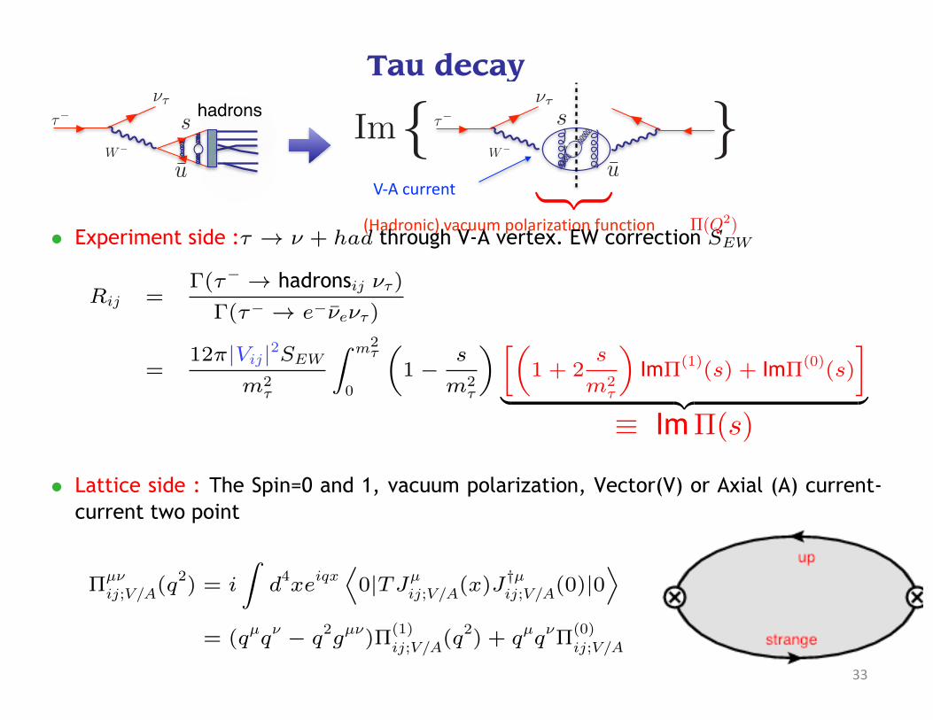
• τ result v.s. non-τ result : more than 3 σ deviation : |Vus| puzzle

• new physics effect?

• incl. analysis uses Finite energy sum rule (FESR)

• pQCD and higher order OPE for FESR:

underestimation of truncation error and/or non-perturbative effects ?

(c.f. alternative FESR approach, R. Hudspith et. al arXiv:1702.01767 )

|us|V0.22 0.225

, PDG 2016l3K 0.0010±0.2237

, PDG 2016l2K 0.0007±0.2254

CKM unitarity, PDG 2016 0.0009±0.2258

s incl., HFLAV Spring 2017→ τ 0.0021±0.2186

, HFLAV Spring 2017νπ → τ / ν K→ τ 0.0018±0.2236

average, HFLAV Spring 2017τ 0.0015±0.2216

HFLAVSpring 2017

3.1�

2

33

Tau decay

Rratio(hadron/lepton)forthefinalstateswithstrangeness-1

τ→ν+hadronsdecaythroughV-Acurrent(weakdecay)

Taudecayexperiment

Rij;V/A ⌘�[�� ⌧Hij;V/A(�)]

�[�� ⌧e��e(�)]

��⌧

u

sW�

hadrons

u

s��⌧

W� •{ }Im

FromunitarityofSmatrix,invariantmatrixelementsarerelatedtothetotalscatteringcrosssectionσ[Opticaltheorem]

V-Acurrent

Thespin0,and1,hadronicvacuumpolarizationfunctionforV/Acurrent-current

Determination of |Vus| from lattice HVP andexperimental hadronic � decay

1 Preliminary

For SM hadronic � decays, a derivative of the ratio Rij;V/A of the decay width into statesproduced hadronic V and A currents with i, j flavors to the electron decay width,

Rij;V/A ⌘ �[�� Hij;V/A(�)]/�[�� e��e(�)] (1)

is related to the spectral functions �(J)ij;V/A with the spin J = 0, 1 by

dRij;V/A

ds=

12�2|Vij|2SEW

m2�

(1 � y�)2�(1 + 2y� )�

0+1ij;V/A(s) � 2y��

0ij;V/A(s)

�, (2)

where y� = s/m2� , SEW is a known short-distance electroweak conrrection. Fig. 1 repre-

sents hadronic � decays. The spectal function is defined as �(J)ij;V/A(s) = 1

� Im�(J)ij;V/A(�s),

where �(J)ij;V/A(�s) is computed from the usual flavor ij vector (V) or axial vector (A)

current-current two-point functions;

�(µ�)ij;V/A(q2) ⌘i

�d4xeiqx�0|T

�Jµ

ij;V/A(x)J†�ij;V/A(0)

�|0�

=(qµq� � q2gµ�)�(1)ij;V/A(Q2) + qµq��

(0)ij;V/A(Q2), (3)

where Jµij;V/A are the V/A currents with flavor ij.

The |Vus| extraction uses an analysis of the us two-point function. From Eq. (2), itshows that the experimental data of dRus;V/A/ds fixes the |Vus|2 and the spectral functioncombination

�1 + 2

s

m2�

�Im�(1)(s) + Im�(0)(s). (4)

The experimental situation for the inclusive � decays is shown in 1. The current statusof |Vus| determination can be found in HFAG-tau summary (See Fig. 2). For the Kaonpole contribution, we assume a simple delta function form as

|Vus|2��

1 + 2s

m2�

�Im�(1)(s) + Im�(0)(s)

�= �(s � m2

k)0.0012299(46). (5)

1

(Hadronic)vacuumpolarizationfunction

�

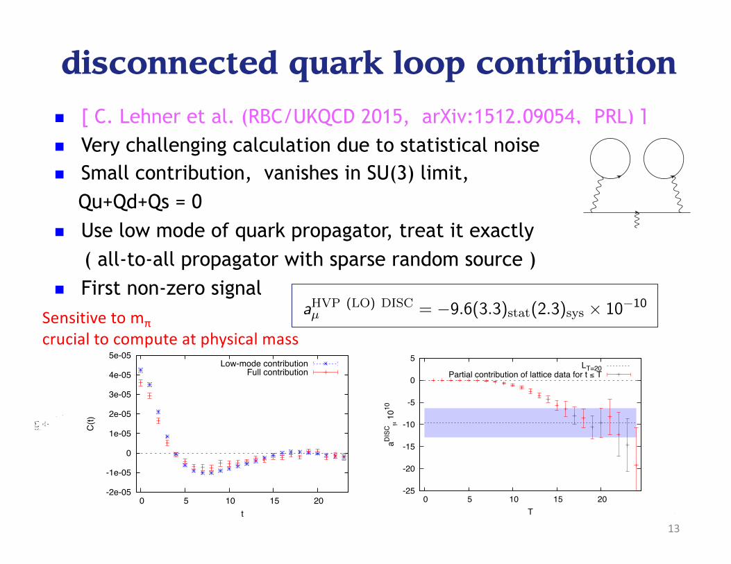
⇧(Q2)• Experiment side :⌧ ! ⌫ + had through V-A vertex. EW correction SEW

Rij =�(⌧� ! hadronsij ⌫⌧)

�(⌧� ! e�⌫e⌫⌧)

=12⇡|Vij|2SEW

m2⌧

Z m2⌧

0

✓1 �

s

m2⌧

◆✓1 + 2

s

m2⌧

◆Im⇧(1)(s) + Im⇧(0)(s)

�

| {z }⌘ Im⇧(s)

• Lattice side : The Spin=0 and 1, vacuum polarization, Vector(V) or Axial (A) current-current two point

⇧µ⌫ij;V/A(q2) = i

Zd4xeiqx

D0|TJµ

ij;V/A(x)J†µij;V/A(0)|0

E

= (qµq⌫ � q2gµ⌫)⇧(1)ij;V/A

(q2) + qµq⌫⇧(0)ij;V/A

Hiroshi Ohki, Friday, June 23 17:50, Seminarios 6+7 [Weak Decays and Matrix Elements] 6

34

Finite Energy Sum Rule (FESR)[Shifman, Vainstein, Zakharov 1979]

• FESR = Optical theorem (Unitarity) + Dispersion relation (Analyticity)

• Optical theorem relate S=-1 spectral function ⇢0/1V/A,ij

(s) and HVP ⇧0/1V/A,ij

(s) for givenquantum number: flavor (us or ud), spin (0 or 1), parity (V or A)

1

⇡Im⇧(s) = ⇢(s)

• Do finite radius contour integral for arbitrary regular weight function w(s)

Zs0

sth

ds⇢(s)w(s) = +i

2⇡

I

|s|=s0

ds⇧(s)w(s)

• Real axis integral is extracted from experimental decayenergy distribution dR⌧/ds

dRij;V/A

ds=

12⇡2|Vij|2SEW

m2⌧

!⌧(s)⇢(s)

Im(s)

Re(s)sth

τexperiment

pQCD

s0

Taku Izubuchi, Columbia Theory Seminar, New York, NY, January 28, 2019 8

35

|Vus| determination from FESR[ E. Gamiz, et al., 2003, 2005, Maltman et al 2006 ]

• Inclusive differencial ⌧ decay rate with wieght w(s)

R!

ij(s0) ⌘Z

s0

sth

dsdRij

ds

!(s/s0)

!⌧(s/m2⌧)

• Take difference between up-down and up-strange channel

�R! =

R!

ud

|Vud|2�

R!

us

|Vus|2

• |Vud| and ms as input, selecting s0 = m2⌧, ! = !⌧(s/s0)

|Vus| =

vuutR!

us(s0)

R!

ud(s0)

|Vud|2 � [�R!(s0)]pQCD

• For s > s0, fixed-order or contour-improved pQCD is used. OPE condensations atdim=4,6 ... are input/assumed. (a source of unaccounted uncertainties)

Im(s)

Re(s)sth

τexperiment

pQCD

s0

Taku Izubuchi, Columbia Theory Seminar, New York, NY, January 28, 2019 10

36

• τ result v.s. non-τ result : more than 3 σ deviation : |Vus| puzzle

• new physics effect?

• incl. analysis uses Finite energy sum rule (FESR)

• pQCD and higher order OPE for FESR:

underestimation of truncation error and/or non-perturbative effects ?

(c.f. alternative FESR approach, R. Hudspith et. al arXiv:1702.01767 )

|us|V0.22 0.225

, PDG 2016l3K 0.0010±0.2237

, PDG 2016l2K 0.0007±0.2254

CKM unitarity, PDG 2016 0.0009±0.2258

s incl., HFLAV Spring 2017→ τ 0.0021±0.2186

, HFLAV Spring 2017νπ → τ / ν K→ τ 0.0018±0.2236

average, HFLAV Spring 2017τ 0.0015±0.2216

HFLAVSpring 2017

3.1�

2

37

Our new method : Combining FESR and Lattice

• If we have a reliable estimate for ⇧(s) in Euclidean (space-like) points, s = �Q2k < 0,

we could extend the FESR with weight function w(s) to have poles there,

Z 1

sth

w(s)Im⇧(s) = ⇡

NpX

k

Resk[w(s)⇧(s)]s=�Q2k

⇧(s) =

✓1 + 2

s

m2⌧

◆Im⇧(1)(s) + Im⇧(0)(s) / s (|s| ! 1)

• For Np � 3, the |s| ! 1 circle integral vanishes.

Re(s)

Im(s)pQCD OPE spectral data

1

XXX

Lattice HVPs


(generalized dispersion relation )

If we have a reliable estimate for Π(s) in Euclidean (space-like) points,

we could extend the FESR with weight function w(s) to have N poles there,

Our strategy

Lattice determination of |Vus| with inclusive hadronic τ decay experiment†

T. Izubuchi,∗1 ∗2 H. Ohki,∗2

The Kobayashi-Maskawa matrix element |Vus| is animportant parameter for flavor physics, which is rele-vant to the search for new physics beyond the standardmodel in particle physics. So far |Vus| has been mostprecisely determined by kaon decay experiments. Asan alternative way, from the τ decay, one can also de-termine |Vus| independently. A conventional methodis to use the so-called finite energy sum rule with poly-nomial weight function ω(s) and the spectral function

ρ(J)V/A with the spin J = 0, 1 as

! s0

0ω(s)ρ(s)ds = − 1

2πi

"

|s|=s0

ω(s)Π(s)ds, (1)

where Π(s) is a hadronic vacuum polarization(HVP)function. Here, ρ(s) on the left hand side is relatedto the differential decay of the τ decay by hadronic Vand A currents with u, s flavors as

dRus;V/A

ds=

12π2|Vus|2SEW

m2τ

(1− yτ )2 (2)

×#(1 + 2yτρ

(0+1)us;V/A − 2yτρ

0us;V/A)

$,

where yτ = s/m2τ , SEW is a known short-distance elec-

troweak correction. The HVP function Π(s) on theright hand side in Eq.(1) is analytically calculated byusing OPE based on perturbative QCD (pQCD). Thus,the momentum s0 should be taken large enough to usea perturbative OPE result. By combining both theinclusive τ decay experiments and pQCD, one can ob-tain |Vus|. Recent analyses suggest that there is 3 σdiscrepancy between two results from the method thatuses the inclusive τ decay and the CKM unitarity con-straint. While there might be a possibility that such adiscrepancy could be explained by new physics effect,we should note that the OPE yields a potential prob-lematic uncertainty in the |Vus| determination from theinclusive hadronic τ decay using the finite energy sumrule a). Thus it is important to reduce the uncertaintyof the QCD part, so that we aim to resolve the so-called|Vus| puzzule.In this report, in order for that purpose, we would

like to propose an alternative method to determine|Vus|, in which we use non-perturbative lattice QCDresults for Π(s) in addition to pQCD. Combing two in-puts, we would expect that more reliable result couldbe obtained. In order to use lattice QCD inputs, we

† All the results shown here are preliminary.∗1 Physics Department, Brookhaven National Laboratory, Up-

ton, NY 11973, USA∗2 RIKEN Nishina Centera) For a recent study of the inclusive τ decay using the finite

energy sum rule, see1).

0 1 2Q1

2 [GeV2]

0.0001

0.001

0.01

0.1

1

N=3, (Q22, Q3

2)=(0.2,0.3)

N=4, (Q22, Q3

2, Q42)=(0.2,0.3,0.4)

N=5, (Q22, Q3

2, Q42, Q5

2)=(0.2,0.3,0.4,0.5)

Fig. 1. Q21 dependence of the ratio of the pQCD to the kaon

pole contribution. For pQCD result, the D = 0 OPE

(Nf = 3) and a conventional value of |Vus| are used.

adopt a different weight function ω(s) which has polesin the Euclidean momentum region. As an illustra-tive example, we take a following weight function asω(s) = 1

(s+Q21)(s+Q2

2)···(s+Q2N )

, where −Q2k < 0 (for

k = 1, ..., N), and N ≥ 3. Taking s0 → ∞ in Eq.(1),we obtain

! ∞

0ρ(s)ω(s)ds =

N%

k

Res&Π(−Q2

k)ω(−Q2k)'. (3)

The lattice result is used for residues on the right handside. The left hand side can be evaluated up to s = m2

τ

from the experimental data, and we use a pQCD re-sult for s > m2

τ . There is an advantage in this method.Since above weight function ω(s) is highly suppressedin high momentum region, so the uncertainty comingfrom pQCD can be reduced. In fact, Fig. 1 shows theweight function dependence of the ratio of the OPEcontribution of the spectrum integral in Eq.(3) to theone from the dominant kaon pole contribution. Asshown in Fig. 1, the OPE contribution can be sup-pressed by adding poles in the weight function.

As a preliminary study, we calculate |Vus| deter-

mined from ρ(0)A . As for the lattice calculation of ρ(0)A ,we use L = 48 lattice result near the physical quarkmassb). Using a weight function with three poles of(Q2

1, Q22, Q

23) = (0.1, 0.2, 0.3), we obtain 0.3% statisti-

cal relative error, which is competitive with previousresults. As a future work, we need to estimate sys-tematic uncertainties such as lattice discretization, un-physical mass, and contributions from other channels,in particular pQCD effects.

References1) P. A. Boyle et al. Int. J. Mod. Phys. Conf. Ser.

35, 1460441 (2014) doi:10.1142/S2010194514604414[arXiv:1312.1716 [hep-ph]].

b) We thank RBC-UKQCD collaboration and Kim Maltmanfor providing lattice HVP and experimental data.

Im(s)

Re(s)sth

τ experiment

pQCD Im(s)

Re(s)sth

τ experiment & pQCD

s0

Lattice HVP

s0 ��

s = �Q2i < 0

(s > m2⌧ )

6

weight function w(s)

• Choice of weight function

w(s) =

NpY

k

1

(s + Q2k)

=X

k

ak1

s + Q2k

, ak =X

j 6=k

1

Q2k � Q2

j

=)X

k

(Qk)Mak = 0 (M = 0, 1, · · · , Np � 2)

• The residue constraints automatically subtracts ⇧(0,1)(0) and s⇧(1)(0) terms.

• For experimental data, w(s) ⇠ 1/sn, n � 3 suppresses

. larger error from higher multiplicity final states at larger s < m2⌧

. uncertanties due to pQCD+OPE at m2⌧ < s

• For lattice, Q2k should be not too small to avoid large stat. error, Q2 ! 0 extrapo-

lation, Finite Volume error. Also not too larger than m2⌧ to make the suppression in

time-like, higher energy, higher multiplicity, region enhanced.

• Comparison of different C, N values provides a self-consistency check for reliableerror.


38

0 0.2 0.4 0.6 0.8 1

C [GeV2]

0.215

0.22

0.225

0.23

0.235

|Vus|

ΓK

[τK

], lattice fK

τ us V+A, N=3τ us V+A, N=4τ us V+A, N=5

Lattice Inclusive determinations

Theory and experimental errors are included.

The result is stable against changes of C and N.

(0.87% total error)N = 4, C = 0.7[GeV2] : |Vus| = 0.2228(15)exp(13)th

(N = 4, � = 0.067 GeV2)

|Vus|

20

39

0.215 0.22 0.225 0.23 0.235 0.24|Vus|

Kl3, PDG 2016

Γ[Kµ2]

3-family unitarity, HT14 |Vud|

τ FB FESR, HFAG17

τ FB FESR, HLMZ17

τ, lattice [N=3, C=0.3 GeV2]



(conventional implementation)

(new implementation, lower : HFAG16 input)

this work(preliminary)

Comparison to from others

All our results (C<1, N=3, 4, 5) are consistent with each other within 1 σ error,

as well as to CKM unitarity.

�K [⌧ ! K⌫⌧ ] : (filled square)

�K [Kµ2] : (empty square)

|Vus|

21

Tau spectral function (vector/axial, Strange=-1) is very welcome !

Hadronic Light-by-Light (HLbL) contributions

Introduction HVP HLbL Summary/Outlook References Perturbative QED in configuration space disconnected diagrams

Hadronic light-by-light (HLbL) scattering

+ + · · ·

Model calculations: (105 ± 26) ⇥ 10�11

[Prades et al., 2009, Benayoun et al., 2014]

Model systematic errors di�cult to quantify

Dispersive approach di�cult, but progress is being made[Colangelo et al., 2014b, Colangelo et al., 2014a, Pauk and Vanderhaeghen, 2014b,

Pauk and Vanderhaeghen, 2014a, Colangelo et al., 2015]

First non-PT QED+QCD calculation [Blum et al., 2015]

Very rapid progress with Pert. QED+QCD [Jin et al., 2015]

Tom Blum (UCONN / RBRC) Progress on the muon anomalous magnetic moment from lattice QCD

40

n Treat all 3 photon propagators exactly (3 analytical photons) , which makes the quark loop and the lepton line connected :

disconnected problem in Lattice QED+QCD -> connected problem with analytic photon

n QED 2-loop in coordinate space. Stochastically sample, two of quark-photon vertex location x,y, z and xop is summed over space-time exactly

n Short separations, Min[ |x-z|,|y-z|,|x-y| ] < R ~ O(0.5) fm, which has a large contribution due to confinement, are summed for all pairs

n longer separations, Min[ |x-z|,|y-z|,|x-y| ] >= R, are done stochastically with a probability shown above ( Adaptive Monte Carlo sampling )

All lepton and photon part produce no noise for given x,y ( Ls = ∞ DWF muon )

Coordinate space Point photon method [ Luchang Jin et al. , PRD93, 014503 (2016) ]

QEDA,QEDB

x y

00.0050.010.0150.020.0250.030.0350.040.0450.05

0 5 10 15 20 25 30 35 40 45

Pro

babilit

y

ceil(r)

32ID

Figure 3. Distribution of the r for 32ID lattice.

For simplicity, we only write local current in above formulas. In actual computation,

however, we need to compute lattice conserved current at xop to ensure the quark loop to

be finite at short distance. We can then use three local current at x, y, and z, provided that

Z3V is multiplied to the final results. See Appendix ???.

We use domain wall action not only for quarks but for the muon as well. We compute

the muon propagators with domain wall height M5 = 1 and infinite Ls. Since all the muon

photon interactions have been explicitly included in the formula, all the muon propagators

are free field fermion propagators. To calculate these free propagators, we can use Fourier

transformations and analytical expressions. So we can enjoys the nice properties without

addition cost compare with the conventional cheaper fermions, e.g. Wilson fermion. We

also use local currents for the photon muon interactions at x′, y′, and z′.

Since we need to sum over all six different permutations of the three internal photons, all

pairs of x, y and combinations of photon polarizations should be computed separately. The

work need to be done for the muon line is proportion to M2. So for large M , the cost for

the free muon propagators can be comparable with the cost for quark propagators. In our

simulations, we usually choose M = 16, which balances the cost for muon and quarks. Also,

M = 16 is not yet too large, so the over all statistics is still roughly proportion to M2.

Above derivation take the limit that tsep → +∞. In practice, if we calculate the QED

part using lattice, we will have finite tsep, which is set to be half of the lattice time extent

11

xop

z

41

Dramatic Improvement !Luchang JinZero External Momentum Transfer Improvement 29/32

-0.04

-0.02

0

0.02

0.04

0.06

0.08

0.1

0.12

0 5 10 15 20 25 30 35

F2(q

2)/(α

/π)3

tsep

q = 2π/L Nprop = 81000q = 0 Nprop = 26568

Figure 20. Phys.Rev.Lett. 114 (2015) 1, 012001. arXiv:1407.2923. Compare with latest method andresult.

• 243× 64 lattice with a−1= 1.747GeV and mπ= 333MeV. mµ= 175MeV.

• For comparison, at physical point, model estimation is 0.08 ± 0.02. The agreement isaccidental, the lattice value has a strong dependence on mµ.

a=0.11 fm, 243x64 (2.7 fm)3, mπ = 329 MeV, mμ =~ 190 MeV, e=1

more than x100 reduced cost !

61

Table 4.10: Results for F2(q2) from applying the conserved and moment methods to the

the 24IL ensemble with mµa = 0.1 using a muon source-sink separation tsep = 32. As

before,pVar = Err

pNconfNprop. We use the conserved current for the external photon

and local currents for the internal photons for both methods. The conserved results are for

q2 = (2⇡/L)2 while the moment methods gives a q2 = 0 result.

Method F2/(↵/⇡)3 Nconf Nprop

pVar

Conserved 0.0825(32) 12 (118 + 128)⇥ 2⇥ 7 0.65

Mom. 0.0804(15) 18 (118 + 128)⇥ 2⇥ 3 0.24

q2 = 0. Since these calculations are less computationally costly than those for QCD, we

can evaluate a number of volumes and lattice spacings (all specified with reference to the

muon mass) and examine the continuum and infinite-volume limits. We can then compare

our results, extrapolated to vanishing lattice spacing and infinite volume, with the known

result calculated in standard QED perturbation theory [9, 10]. This QED calculation serves

both as a demonstration of the capability of lattice methods to determine such light-by-light

scattering amplitudes and as a first look at the size of the finite-volume and nonzero-lattice-

spacing errors.

In Fig. 4.6 we show results for F2(0) computed for three di↵erent lattice spacings, i.e.

three di↵erent values of the input muon mass in lattice units, but keeping the linear size of

the system fixed in units of the muon mass. The data shown in Fig. 4.6 are also presented

in Table 4.11. We use two extrapolation methods to obtain the continuum limit. The first,

shown in the figure, uses a quadratic function of a2 to extrapolate to a2 = 0. The second

makes a linear extrapolation to a2 = 0 using only the two leftmost points for each of the

three values of mµL. The coe�cients for the quadratic-in-a2 fits shown in Fig. 4.6 as well as

those for the linear-in-a2 fits are given in tabular form in Tables. 4.12 and 4.13.

Conserved External Current Improvement 22/32

• In previous setup, noise will remain relatively constant in large volume, but would blowup if the external momentum transfer q becomes small.

u(p′)Γµ(p′, p)u(p) = u(p′)

!F1(q2)γµ+ i

F2(q2)4m

[γµ, γν]qν

"u(p) (12)

F2(0) =gµ− 22

≡ aµ (13)

• To make the noise also vanish when q → 0, we need the external current be exactlyconserved, configuration by configuration.

• To prove Ward identity, we need to compute all possible external photon insertion options.

xsrc xsnky′,σ

′z′, ν

′ x′, ρ

′

xop, µ

z, ν

y,σ x, ρ

xsrc xsnky′,σ

′z′, ν

′ x′, ρ

′

xop, µ

z, ν

y,σ x, ρ

xsrc xsnky′,σ

′z′, ν

′ x′, ρ

′

xop, µ

z, ν

y,σ x, ρ

Figure 14. All three different possible insertions for the external photon. They are equal to each otherafter stochastic average. 5 other possible permutations of the three internal photons are not shown.tsep

2.2 fm

42

SU(3) hierarchies for d-HLbL

n At ms=mud limit, following type of disconnected HLbLdiagrams survive Qu + Qd + Qs = 0

n Physical point run using similar techniques to c-HLbL.

n other diagrams suppressed byO(ms-mud) /3 and O( (ms-mud)2 )

Muon g − 2 Light by Light

by Luchang Jin

xsrc xsnkz′,κ

′y′,σ

′ x′, ρ

′

xop, ν

z,κy,σ x, ρ

Figure 1. Disconnected Light by Light diagrams. There are other possible permutations.

1 Method outline

• Use one configuration to compute 32 point source propagators and perform HVP like con-traction. Store the average of the results, Πρ,σ

avg(r), and later we would subtract it from otherHVP like contraction computed using other configurations.

Πρ,σavg(r) =

1N

!

k=1

N

{−Tr[γρSq(xk, xk + r)γσSq(xk + r, xk)]} (1)

• Start with point source x, compute point source quark propagators and photon x→ x′.

• Compute the local current for all possible y, Πρ,σ(x, y) (subtract Πρ,σavg(x, y) from this value)

Πρ,σ(x, y) = −Tr[γρSq(x, y)γσSq(y, x)]−Πρ,σavg(y −x) (2)

• Optional subtraction: Ideally, the sum of the current over space time should be zero. Sincewe use local current, this is not strictly true. But we can introduce Πρ,σ

′ (x, y) where

Πρ,σ′ (x, y) = Πρ,σ(x, y)− δx,y

!

y ′

Πρ,σ(x, y ′) (3)

Should try to see if this trick work for connected LbL calculation.

• Use the current computed above as a source and construct photon y→ y ′

• Use the two photons constructed above and compute the muon line with sequential sourcefinally contract at z ′ with local current. Note that this procedure should be performed for allpossible permutations of the three photons. The muon source and sink separation is usuallytaken to be half of the lattice time extent, and the source and sink positions are chosen sothat x is in the middle of them xt = ((xsrc)t +(xsnk)t)/2.

• Use the local current at all possible z ′ construct photon z ′→ z

1

68

Figure 5.1: Leading order diagram, survives in SU(3) limit.

xsrc xsnkz0,0 y0,�0 x0, ⇢0

xop, ⌫

z, y,� x, ⇢

Figure 5.2: Next to leading order diagrams. O(ms �ml), vanishes in SU(3) limit.

xsrc xsnky0,�0 x0, ⇢0 z0,0

xop, ⌫

z,y,� x, ⇢

xsrc xsnky0,�0 z0,0 x0, ⇢0

xop, ⌫

z,y,� x, ⇢

diagrams, the signal has to come from a subtle gluon interactions between the two quark

loops, which can only be discovered by gauge averaging. As a result, although the signal

should be exponentially suppresed when |r| = |x � z| become large just as the connected

diagram, the noise remains constant for arbitrary |r|. Since the formula involve summation

over r, one can expect a lot of noises come from the large |r| region, and will become larger

if we increase the volume. However, the independence of these two loops also provide some

benefit. The contraction at y position will not depend on the position of z, thus the M2 trick

can be applied without recomputing the muon part. So, we obtained order M2 combinations

of samples with no additional cost, where M is the number of point source quark propagators

69

Figure 5.3: Even higher order diagrams.


xop, ⌫

z, y,� x, ⇢

xsrc xsnky0,�0 x0, ⇢0 z0,0

xop, ⌫

z,y,� x, ⇢


xop, ⌫

z, y,� x, ⇢

computed for each configuration.

5.2 Infinite volume limit

Normally, the finite volume e↵ects in lattice QCD calculations are exponentially suppressed

by L, the linear size of the lattice volume times m⇡, the energy of lowest energy eigen-state

of QCD. For example, the points x, y, z, which appears in Eq. (3.6), are directly connected

to on the quark loop. The finite volume e↵ects introduced when limiting these points in a

finite size lattice are exponentially suppressed. However, in the light-by-light calculation,

there are also QED finite volume e↵ects. The QED finite volume e↵ects enter only through

Eq. (3.7), which include everything except the quark loop. We repeat the equation below:

G⇢�(x, y, z, xsnk, xsrc) =X

x0,y0,z0

G⇢⇢0(x, x0)G��0(y, y0)G0(z, z0)

·

hSµ (xsnk, x

0) �⇢0Sµ(x0, z0)�0Sµ(z

0, y0)��0Sµ (y0, xsrc)

+Sµ (xsnk, z0) �0Sµ(z

0, x0)�⇢0Sµ(x0, y0)��0Sµ (y

0, xsrc)

+four other permutationsi. (5.1)

The summation variables x0, y0, z0 in above equation can move freely along the muon line,

only connected to the quark loop by massless photons. Thus, Eq. (5.1), when evaluated

(ms-mud)0

(ms-mud)/3 (ms-mud)2

43

140 MeV Pion, connected and disconnected LbL results

[ Luchang Jin et al. , Phys.Rev.Lett. 118 (2017) 022005 ]n left: connected, right : leading disconnected

n Using AMA with 2,000 zMobius low modes, AMA

139MeV Pion 483× 96 Lattice 21/32

-0.005

0

0.005

0.01

0.015

0.02

0.025

0.03

0 5 10 15 20

F2(0)/(α

/π)3

|r|

48I

-0.006-0.005-0.004-0.003-0.002-0.001

00.0010.0020.0030.004

0 5 10 15 20

F2(0)/(α

/π)3

|r|

48I

Figure 15. 483 × 96 lattice, with a−1 = 1.73GeV, mπ = 139MeV, mµ = 106MeV. Left: connecteddiagrams contribution. Right: leading disconnected diagrams contribution.

• We use Lanczos, AMA, and zMobius techniques to speed up the computations.

• 65 configurations are used. They each are separated by 20 MD time units.

gµ − 22

!

!

!

!

cHLbL

= (0.0926± 0.0077)×"

α

π

#

3=(11.60± 0.96)× 10−10 (17)

gµ − 22

!

!

!

!

dHLbL

= (−0.0498± 0.0064)×"

α

π

#

3=(−6.25± 0.80)× 10−10 (18)

gµ − 22

!

!

!

!

HLbL

= (0.0427± 0.0108)×"

α

π

#

3=(5.35± 1.35)× 10−10 (19)

139MeV Pion 483× 96 Lattice 21/32

-0.005

0

0.005

0.01

0.015

0.02

0.025

0.03

0 5 10 15 20

F2(0)/(α

/π)3

|r|

48I

-0.006-0.005-0.004-0.003-0.002-0.001

00.0010.0020.0030.004

0 5 10 15 20

F2(0)/(α

/π)3

|r|

48I

Figure 15. 483 × 96 lattice, with a−1 = 1.73GeV, mπ = 139MeV, mµ = 106MeV. Left: connecteddiagrams contribution. Right: leading disconnected diagrams contribution.

• We use Lanczos, AMA, and zMobius techniques to speed up the computations.

• 65 configurations are used. They each are separated by 20 MD time units.

gµ − 22

!

!

!

!

cHLbL

= (0.0926± 0.0077)×"

α

π

#

3=(11.60± 0.96)× 10−10 (17)

gµ − 22

!

!

!

!

dHLbL

= (−0.0498± 0.0064)×"

α

π

#

3=(−6.25± 0.80)× 10−10 (18)

gµ − 22

!

!

!

!

HLbL

= (0.0427± 0.0108)×"

α

π

#

3=(5.35± 1.35)× 10−10 (19)

( statistical error only )

44

1.4 fm

PRD93(2015)014503 (RBC/UKQCD):

New sampling strategy with 10x reduced noise for same cost (red versus black):

MµLbL(q) remains constant, if we try to extract F2(q2) using Eq ???, the noise for F2(q2) would still

go like 1/ q. This can be a serious problem because we are really interested in the value of F2(q2)in the q!0 limit. Since we always evaluate the amplitude at q =2⇡/L, the noise for F2(q2) wouldbe proportion to L.

xsrc xsnky�, �� z�, �� x�, ��

xop, µ

z, �

y, � x, �

xsrc xsnky�, �� z�, �� x�, ��

xop, µz, �

y, � x, �

xsrc xsnky�, �� z�, �� x�, ��

xop, µz, �

y, � x, �

Figure 22. All three different possible insertions for the external photon. They are equal to each otherafter stochastic average. Just like Fig ???, 5 other possible permutations of the three internal photons arenot shown. (L) This is the diagram that we have already calculated. (M) We need to compute sequentialsource propagators at xop for each polarizations of the external photon. (R) We also need to compuatesequential source propagators at xop, but with the external photon momentum in opposite direction, sincewe need use �5-hermiticity to reverse the direction of the propagators, which reverses the momentum of theexternal photon as well.

The reason that amplitude is proportion to q is the external photon is couple to a conservedcurrent of a quark loop. Current conservation ensures that the amplitude vanishes if the externalmomentum is zero. Although we implemented exact conserved current at xop and sum it over theentire space time in the method described above, we didn’t compute all three possible insertions forthe external photon. So the current is only truly conserved after stochastic average over x and y. Asa result, the noise would not be zero when q =0. To fix this, we just need to compute all diagramsin above figure, then the noise would be proportion to q as well.1 These additional diagrams arealso computationally accessible. We only need to compute sequential propagators for each possiblepolarizations and momentums of the external photon. We normally compute three polarizationdirections x, y, and t, which are perpendicular to the direction of the external momentum z. Thiswould be six times more work for the quark loop part of the computation, but the cost for themuon part remains unchanged. We can adjust M to rebalance the cost, so the over all cost increasemight not be significant but the potential gain can be large especially in a large volume.

There is also another trick. When we sum over z to get the exact photon, we don’t have to sum overthe entire volume, instead, we only sum over the region where |x� y |< |x�z | and |x� y |< |y �z |.2This trick will enhance the signal in short distance but suppress signal and noise in long distancewhere the distance. This trick is called MinDis in the tables blow.

4.1 Zero Total Current Prove

Here we try to prove that the sum of a conserved current is zero if it vanishes at the boundary.

Given:

�µjµ = 0, (19)

1. Although the current conservation is exact, in finite lattice with periodic boundry condition, around the worldeffects will contribute to the noise even when the external momentum is zero. But this noise is suppressed expo-nentially in the large volume limit. In summary, in the small q and large volume limit, the noise is roughlyO(q)+ O

�e�m�L/2

�.

2. We need multiply some different factors when two edges happened to have the same length.

19

Figure 9. A comparison of the results for F2(q2)/(�/⇡)3 obtained in the original lattice QCD

cHLbL calculation [17] (diamonds) with those obtained on the same gauge field ensemble using the

moment method presented here (circles). The points from the original subtraction method with

q2 = (2⇡/24)2 = (457MeV)2 were obtained from 100 configurations and the evaluation of 81,000

point-source quark propagators for each value of the source-sink separation tsep. In contrast, the

much more statistically precise results from the moment method required a combined 26,568 quark

propagator inversions for both values of tsep and correspond to q2 = 0. The moment method value

for tsep = 32 is listed in Tab. IX.

make use of the most e�ective of the numerical strategies discussed above: the use of exact

photon propagators and the position-space moment method to determine F2 evaluated at

q2 = 0. Since these calculations are less computationally costly than those for QCD we

can evaluate a number of volumes and lattice spacings (all specified with reference to the

muon mass) and examine the continuum and infinite volume limits. We can then compare

our results, extrapolated to vanishing lattice spacing and infinite volume, with the known

result calculated in standard QED perturbation theory [33, 34]. This QED calculation both

serves as a demonstration of the capability of lattice methods to determine such light-by-light

scattering amplitudes and as a first look at the size of the finite-volume and non-zero-lattice-

spacing errors.

In Fig. 10 we show results for F2(0) computed for three di�erent lattice spacings, i.e.

39

�

�

��↵

A

A

AAU

Stochastically evaluate the sum over vertices x and y :

I Pick random point x on lattice

I Sample all points y up to a specific distance r = |x � y |

I Pick y following a distribution P(|x � y |) that is peaked at short distances

12 / 20

r = |x-y|

Continuum / infinite volume extrapolation

n Discretization error 1/a = 2.7, 1.4 GeV at physical quark mass

n Finite volume L = 4.8, 6.4, 9.6 fm at 1/a=1 GeV at physical mass

45

135MeV pion on 64I ensemble (prelim) 28/50

This is slightly partial quenched calculation performed on the 139MeV pion mass ensemble.

0

5

10

15

20

25

0 0.5 1 1.5 2 2.5

aµ×

1010

r (fm)

48I con64I con

48I-64I con

−18

−16

−14

−12

−10

−8

−6

−4

−2

0

0 0.5 1 1.5 2 2.5 3 3.5 4 4.5

aµ×

1010

r (fm)

48I discon64I discon

48I-64I discon

• Left: connected diagrams. Right: leading disconnected diagrams.

• 483× 96 lattice, with a−1= 1.73GeV, mπ= 135MeV (corrected from 139MeV).

• 643× 128 lattice, with a−1= 2.36GeV, mπ= 135MeV.

aµcHLbL = (16.94± 3.77)× 10−10 (27)

aµdHLbL = (−12.31± 3.39)× 10−10 (28)

aµHLbL = (4.63± 4.44)× 10−10 (29)

connecteddisconnectedInfinite volume limit (prelim) 31/50

• MDWF+Iwasaki: continuum limit (5.4fm)

• MDWF+DSDR: a−1=1.015GeV: 243×64 (4.8fm), 323×64 (6.4fm), 483×64 (9.6fm).

• MDWF+DSDR: a−1= 1.371GeV: 323× 64 (4.6fm).

F2(a, L) = F2

!

1− c1(mµL)2

"

(1− c2 a2) (34)

0

5

10

15

20

25

30

0 0.05 0.1 0.15 0.2

a µ×10

10

1/(mµL)2

48I-64I24D32D48D

32Dfine

−20

−15

−10

−5

0

0 0.05 0.1 0.15 0.2

a µ×10

10

1/(mµL)2

48I-64I24D32D

32Dfine

Connected diagrams Disconnected diagrams

aµcHLbL = (26.12± 3.87stat± 0.28sys,a2)× 10−10 (35)

aµdHLbL = (−12.87± 2.27stat± 1.63sys,a2)× 10−10 (36)

aµHLbL = (13.24± 4.40stat± 1.91sys,a2)× 10−10 (37)

HLbL( connected + leading disconnected)

n The connected + leading disconnected contribution

n continuum, infinite volume limit

n preliminary results [ Luchang Jin, Schwinger Fest 2018-12-04 ]

My own calculation: h3 ⌅ [�10, 10] GeV�2

X aµ(LbL; X) ⇥ 1011

⇥0, �, �⇤ 93.91 ± 12.40 a1, f ⇤1, f1 28.13 ± 5.63 a0, f ⇤0, f0 �5.98 ± 1.20

JN09 based on Nyffeler 09:

aLbL;hadµ = (116 ± 39) ⇥ 10�11

Summary of resultsContribution BPP HKS KN MV PdRV N/JN

⇥0, �, �⇤ 85±13 82.7±6.4 83±12 114±10 114±13 99±16⇥,K loops �19±13 �4.5±8.1 � 0±10 �19±19 �19±13

axial vectors 2.5±1.0 1.7±1.7 � 22± 5 15±10 22± 5scalars �6.8±2.0 � � � �7± 7 �7± 2

quark loops 21± 3 9.7±11.1 � � 2.3 21± 3

total 83±32 89.6±15.4 80±40 136±25 105±26 116±39

F. Jegerlehner SFB/TR 09 Meeting, Aachen, November 14, 2011 92

F. Jegerlehner , x 1011

46

Infinite volume limit (prelim) 31/50



• MDWF+DSDR: a−1= 1.371GeV: 323× 64 (4.6fm).

F2(a, L) = F2

!

1− c1(mµL)2

"

(1− c2 a2) (34)

0

5

10

15

20

25

30

0 0.05 0.1 0.15 0.2

aµ×10

10

1/(mµL)2

48I-64I24D32D48D

32Dfine

−20

−15

−10

−5

0

0 0.05 0.1 0.15 0.2

aµ×10

10

1/(mµL)2

48I-64I24D32D

32Dfine




aµHLbL = (13.24± 4.40stat± 1.91sys,a2)× 10−10 (37)

Infinite volume limit (prelim) 31/50



• MDWF+DSDR: a−1= 1.371GeV: 323× 64 (4.6fm).

F2(a, L) = F2

!

1− c1(mµL)2

"

(1− c2 a2) (34)

0

5

10

15

20

25

30

0 0.05 0.1 0.15 0.2

a µ×10

10

1/(mµL)2

48I-64I24D32D48D

32Dfine

−20

−15

−10

−5

0

0 0.05 0.1 0.15 0.2

a µ×10

10

1/(mµL)2

48I-64I24D32D

32Dfine




aµHLbL = (13.24± 4.40stat± 1.91sys,a2)× 10−10 (37)

Summary & Perspectivesn HVP

• New methods using low mode for connected at physical quark mass, • disconnected quark loop at physical quark mass, QED and IB studies are included• Combining with R-ratio experiment data for cross-check and improvement => 0.4 % error • Eventually the window will be enlarged for a pure LQCD prediction (currently 2.6 % error)

• Significant improvements is in progress for statistical error using 2π and 4π (!) states in addition to EM current (GEVP, GS-parametrization)

• Checking finite volume and discretization error as well as Isospin V effects

n τ input for g-2 HVP

We could compute Inclusive hadron cross sections at Euclidean q^2from the first principle Lattice QCD with Isospin breaking effects

n τ inclusive analysis and Vus

|Vus| from tau inclusive could becompetitive to Kaon determination

n HLbL• computing connected and leading disconnected diagrams, take continue & infinite

volume limits• preliminary result not very different from the model results (Glasgow consensus)• pi0 pole contribution & higher order disconnected diagrams are in progress

47

Improved τ spectral functionswill be very valuable

48

Results KNT18 update

KNT18 aSMµ update

Alex Keshavarzi (UoL) ahad, VPµ from KNT18 12th February 2018 20 / 22

160 170 180 190 200 210 220

(aµ

SM x 1010)−11659000

DHMZ10

JS11

HLMNT11

FJ17

DHMZ17

KNT18

BNL

BNL (x4 accuracy)

3.7σ

7.0σ

49

g-2 HVP Workshop, KEK 13/02/2018 25

• BABAR and KLOE measurements most precise to date, but in poor agreement

• Others are in between, but not precise enough to decide

• No progress achieved in understanding the reason(s) of the discrepancy

• consequence: accuracy of combined results degraded

• imperative to improve accuracy of prediction (forthcoming g-2 results at FNAL, J-PARC)

• Other efforts at VEPP-2000 underway

• Design a new independent BABAR analysis

M. Davier ISR BABAR g-2

The BABAR/KLOE discrepancy for ppg(g)

Cross check, combine, and improve by LQCD data

Precession of Mercury and GR

50

discrepancy recognized since 1859

1915 by-then New physics

GR revolu?on

precession of perihelion

[Luchang Jin’s analogy]

College Park, MD 2011 PROCEEDINGS of the NPA 1

The Theory of Mercury’s Anomalous Precession Roger A. Rydin

Associate Professor Emeritus of Nuclear Engineering, University of Virginia 626 Cabell Avenue, Charlottesville, VA 22903-2011

e-mail: [email protected]

Urbain Le Verrier published a preliminary paper in 1841 on the Theory of Mercury, and a definitive paper in 1859. He discovered a small unexplained shift in the perihelion of Mercury of 39” per century. The results were corrected in 1895 by Simon Newcomb, who increased the anomalous shift by about 10%. Albert Einstein, at the end of his 1916 paper on General Relativity, gave a specific solution for the perihelion shift which exactly matched the discrepancy. Dating from the 1947 Clemence review paper, that explanation and precise value have remained to the present time, being completely accepted by theoretical physicists as absolutely true. Modern numerical fittings of planetary orbits called Ephemerides contain linearized General Relativity corrections that cannot be turned off to see if discrepancies between observation and computation still exist of the magnitude necessary to support the General Relativity estimates of the differences.

The highly technical 1859 Le Verrier paper was written in French. The partial translation given here throws light on Le Verrier’s analysis and thought processes, and points out that the masses he used for Earth and Mercury are quite different from present day values. A 1924 paper by a professor of Celestial Mechanics critiques both the Einstein and the Le Verrier analyses, and a 1993 paper gives a different and better fit to some of Le Verrier’s data. Nonetheless, the effect of errors in planet masses seems to give new condition equations that do not change the perihelion discrepancy by a large amount. The question now is whether or not the excess shift of the perihelion of Mercury is real and has been properly explained in terms of General Relativity, or if there are other reasons for the observations. There are significant arguments that General Relativity has not been proven experimentally, and that it contains mathematical errors that invalidate its predictions. Vankov has analyzed Einstein’s 1915 derivation and concludes that when an inconsistency is corrected, there is no perihelion shift at all!

1. Introduction In his 1916 paper on General Relativity [1], Albert Einstein

announced that he had explained the apparent anomalous shift in the perihelion of Mercury, discovered by the French astrophysicist, Urbain Le Verrier [2, 3] in 1859 and corrected slightly by Simon Newcomb [4, 5] in 1895. As the accompanying table shows, the total observed precession of 5600 arc seconds per century is made up mostly by a coordinate transformation, whereas the calculation of the effects of other planets remains at roughly the 1895 values, and Einstein’s correction is taken as a real effect that exactly explains the difference.

Amount (arc-sec/century)

Cause

5025.6 Coordinate (due to precession of equinoxes) 531.4 Gravitational tugs of the other planets 0.0254 Oblateness of the sun (quadrupole moment)

42.98±0.04 General relativity 5600.0 Total 5599.7 Observed

Fig. 1. Sources of the Precession of Perihelion for Mercury

Fig. 1 is taken from a 1947 paper by Clemence [6], which is essentially the definitive analysis of all Mercury data taken up to that time. Clemence says, “It is at once evident that the effect can be detected most easily in the motion of Mercury. Indeed, Einstein's announcement of the general theory of relativity in its definitive form was immediately hailed by some astronomers as

explaining a previously unaccountable discrepancy between the observed and theoretical motions of this planet. Others were, however, intuitively opposed to relativity, and they directed attention to a small discrepancy yet remaining as evidence that the theory of relativity could not be correct: the relativists contended that the small remaining discrepancy was due to errors either in the observations or in the classical theory of the motion. In justice it should be said that the questions involved are not simple ones, but are complicated by three causes:

1. Observations of Mercury are among the most difficult in positional astronomy. They have to be made in the daytime, near noon, under unfavorable conditions of the atmosphere; and they are subject to large systematic and accidental errors arising both from this cause and from the shape of the visible disk of the planet.

2. The planet's path in Newtonian space is not an ellipse but an exceedingly complicated space-curve due to the disturbing effects of all of the other planets. The calculation of this curve is a difficult and laborious task, and significantly different results have been obtained by different scientists.

3. The observations cannot be made in the Newtonian frame of reference. They are referred to the moving equinox, that is, they are affected by the precession of the equinoxes, and the determination of the precessional motion is one of the most difficult problems of positional astronomy, if not the most difficult. In light of all these hazards it is not surprising that a difference of opinion could exist regarding the closeness of agreement between the observed and theoretical motions.”

http://worldnpa.org/abstracts/abstracts_6066.pdf

Known physics

n Fermion’s energy in the external magnetic field:

n Magnetic moment Lande g-factor tree level value 2n 1928 P.A.M. Dirac “Quantum Theory of Electron”

Dirac equation (relativity, minimal gauge interaction)

n Non-relativistic and weak constant magnetic fieldlimits of the Dirac equation :

EQUATIONS

N. YAMADA

V (x) = −µl · B(1)

µl = gle sl

2ml(2)

al =gl − 2

2(3)

aµ = (11 659 182.8 ± 4.9) × 10−10(4)

(5)

Date: July 4, 2012.1

EQUATIONS

N. YAMADA

V (x) = −µl · B(1)

µl = gle

2mlSl(2)

al =gl − 2

2(3)

aµ = (11 659 182.8 ± 4.9) × 10−10(4)

(5)

Date: July 4, 2012.1

Anomalous magnetic momentBS

51

�i~@ @t

=

r2

2m+

e

2m

⇣~L+ 2~S

⌘· ~B

�

<latexit sha1_base64="(null)">(null)</latexit><latexit sha1_base64="(null)">(null)</latexit><latexit sha1_base64="(null)">(null)</latexit><latexit sha1_base64="(null)">(null)</latexit>

gl = 2<latexit sha1_base64="(null)">(null)</latexit><latexit sha1_base64="(null)">(null)</latexit><latexit sha1_base64="(null)">(null)</latexit><latexit sha1_base64="(null)">(null)</latexit><latexit sha1_base64="(null)">(null)</latexit><latexit sha1_base64="(null)">(null)</latexit><latexit sha1_base64="(null)">(null)</latexit><latexit sha1_base64="(null)">(null)</latexit><latexit sha1_base64="(null)">(null)</latexit><latexit sha1_base64="(null)">(null)</latexit><latexit sha1_base64="(null)">(null)</latexit><latexit sha1_base64="(null)">(null)</latexit><latexit sha1_base64="(null)">(null)</latexit>

(for Dirac Fermion l = e, μ, τ, …. )

i[@µ � ieAµ(x)]�µ (x) = m (x)

<latexit sha1_base64="(null)">(null)</latexit><latexit sha1_base64="(null)">(null)</latexit><latexit sha1_base64="(null)">(null)</latexit><latexit sha1_base64="(null)">(null)</latexit>

SM Theory

n QED, hadronic, EW contributions

+ ...+=

✕ ✕ ✕

+ + + ...✕ ✕

+ + + ...

✕ ✕

QED (5-loop)Aoyama et al. PRL109,111808 (2012)

Hadronic vacuum polarizaEon (HVP)

Hadronic light-by-light (Hlbl)

Electroweak (EW)Knecht et al 02Czarnecki et al. 02

+ + …

+ + + …

muon’s anomalous magnetic moment

• One of the most precisely determined numbers, starting from the construction of QED.

�

�

µ µ

�

� �

µ µhad

�

W W

⇤

µ µ

Hadronic light-by-light scattering contribution to the muon g� 2 from lattice QCD Masashi Hayakawa

could be estimated by purely theoretical calculation. So far, it has been calculated only based onthe hadronic picture [7, 8]. Thus the first principle calculation based on lattice QCD is particularlydesirable.

!

l1l2

Figure 1: hadronic light-by-light scattering contribution to the muon g� 2

The diagram in Fig. 1 evokes the following naive approach; we calculate repeatedly the cor-relation function of four hadronic electromagnetic currents by lattice QCD with respect to twoindependent four-momenta l1, l2 of off-shell photons, and integrate it over l1, l2. Such a task is toodifficult to accomplish with use of supercomputers available in the foreseeable future.

Here we propose a practical method to calculate the h-lbl contribution by using the lattice(QCD + QED) simulation; we compute

⇤ quark ⌅

QCD+quenched QEDA

�⇤

quark

⌅

QCD+quenched QEDB⇤ ⌅

quenched QEDA

, (2)

amputate the external muon lines, and project the magnetic form factor, and divide by the factor3. In Eq. (2) the red line denotes the free photon propagator D!�(x, y) in the non-compact lat-tice QED solved in an appropriate gauge fixing condition. The black line denotes the full quarkpropagator Sf (x, y;U, u) for a given set of SU(3)C gauge configuration

�Ux,!

⇥and U(1)em gauge

configuration�ux,!

⇥, where the sum over relevant flavors f is implicitly assumed. The blue line

represents the full muon propagator s(x, y; u). The average ⇥, ⇤ above means the one over theunquenched SU(3)C gauge configurations and/or the quenched U(1)em gauge configurations 1 asspecified by the subscript attached to it. Since two statistically independent averages overU(1)emgauge configurations appear in the second term, they are distinguished by the labels A, B.

1For the unquenched QCD plus quenched QED to respect the gauge invariance of QED, the electromagnetic chargesof sea quarks are assumed to be zero.

PoS(LAT2005)353

353 / 3

aµ =g � 2

2= (116 592 089 ± 54 ± 33) ⇥ 10�11 BNL-E821

[Andreas Hoecker, Tau 2010, arXiv:1012.0055 [hep-ph]]

Contribution Result (⇥10�11).QED (leptons) 116 584 718.09 ± 0.15HVP (lo) 6 923.± 42HVP (ho) -97.9 ± 0.9HLBL 105.± 26EW 154.± 2

Total SM 116 591 802 ± 42HVP(lo) ± 26HLBL ± 02 (49tot).

• 287 ± 80 or 3.6⇥ difference between experiment and SM prediction.

E989 at FNAL is to reduce the total experimental error by,at least, a factor of four over E821, or 0.14 ppm !

Taku Izubuchi, USQCD All Hands Meeting, JLab, May 6, 2011 20

IntroductionThe hadronic vacuum polarization (HVP) contribution (O(↵2))

The hadronic light-by-light (HLbL) contribution (O(↵3))Summary/Outlook

The magnetic moment of the muon

In interacting quantum (field) theory g gets corrections

qp1 p2

+qp1 p2

k

+ . . .

�µ! �µ(q) =

✓�µ F1(q

2) +i �µ⌫ q⌫2m

F2(q2)

◆

which results from Lorentz and gauge invariance when the muon ison-mass-shell.

F2(0) =g � 2

2⌘ aµ (F1(0) = 1)

(the anomalous magnetic moment, or anomaly)

Tom Blum (UConn / RIKEN BNL Research Center) Hadronic contributions to the muon g-2 from lattice QCD

IntroductionThe hadronic vacuum polarization (HVP) contribution (O(↵2))

The hadronic light-by-light (HLbL) contribution (O(↵3))Summary/Outlook

The magnetic moment of the muon

Compute these corrections order-by-order in perturbation theory byexpanding �µ(q2) in QED coupling constant

↵ =e2

4⇡=

1

137+ . . .

Corrections begin at O(↵); Schwinger term = ↵

2⇡= 0.0011614 . . .

hadronic contributions ⇠ 6 ⇥ 10�5 times smaller (leading error).

Tom Blum (UConn / RIKEN BNL Research Center) Hadronic contributions to the muon g-2 from lattice QCD

52

Hadronic contributions to muon g-2

Documents

Transcript of Hadronic contributions to muon g-2