Performance of the ALICE muon spectrometer. Weak boson ...

HAL Id: tel-00198703https://tel.archives-ouvertes.fr/tel-00198703

Submitted on 17 Dec 2007

HAL is a multi-disciplinary open accessarchive for the deposit and dissemination of sci-entific research documents, whether they are pub-lished or not. The documents may come fromteaching and research institutions in France orabroad, or from public or private research centers.

L’archive ouverte pluridisciplinaire HAL, estdestinée au dépôt et à la diffusion de documentsscientifiques de niveau recherche, publiés ou non,émanant des établissements d’enseignement et derecherche français ou étrangers, des laboratoirespublics ou privés.

Performance of the ALICE muon spectrometer. Weakboson production and measurement in heavy-ion

collisions at LHC.Zaida Conesa del Valle

To cite this version:Zaida Conesa del Valle. Performance of the ALICE muon spectrometer. Weak boson productionand measurement in heavy-ion collisions at LHC.. Nuclear Theory [nucl-th]. Université de Nantes;Universitat Autónoma de Barcelona, 2007. English. �tel-00198703�

https://tel.archives-ouvertes.fr/tel-00198703

https://hal.archives-ouvertes.fr

UNIVERSITE DE NANTESFACULTE DES SCIENCES ET TECHNIQUES

————-ECOLE DOCTORALE

SCIENCES ET TECHNOLOGIES DE L’INFORMATION ET DES MATERIAUX

Annee : 2007N◦ attribue par la bibliotheque

Performance of the ALICE muon spectrometer.

Weak boson production and measurement in

heavy-ion collisions at LHC.

THESE DE DOCTORAT

Discipline : Physique Nucleaire

Specialite : Physique des Ions Lourds

Presentee et soutenue publiquement par

Zaida CONESA DEL VALLE

Le 12 juillet 2007, devant le jury ci-dessous

President K. WERNER, Professeur, Universite de Nantes, SUBATECH, Nantes

Rapporteurs E. VERCELLIN, Professeur, Universita degli Studi di Torino, Torino

D. G.-D’ENTERRIA ADAN, Charge de recherche, CERN, Geneve

Examinateurs E. AUGE, Professeur, Universite Paris-Sud XI, LAL, Orsay

H. BOREL, Ingenieur de recherche, CEA, Saclay

Directeurs de these : G. MARTINEZ GARCIA, Charge de recherche, CNRS, SUBATECH Nantes

F. FERNANDEZ MORENO, Professeur, Universitat Autonoma de Barcelona

N◦ ED 366-312

Performance du spectrometre a muons d’ALICE.

Production et mesure des bosons faibles dans des

collisions d’ions lourds aupres du LHC.

——————–

Performance of the ALICE muon spectrometer. Weak boson

production and measurement in heavy-ion collisions at LHC.


SUBATECH, Nantes (France), 2007

Performance of the ALICE muon spectrometer. Weak

boson production and measurement in heavy-ion

collisions at LHC.

TESIS DOCTORAL

Zaida Conesa del Valle

Directors de tesis:

Gines Martınez Garcıa, SUBATECH Nantes

Francisco Fernandez Moreno, Universitat Autonoma de Barcelona

Grup de Fısica de les Radiacions, Bellaterra (Spain), 2007

Contents

Acknowledgements xi

Abstract xiii

I Introduction 1

1 Studying the Quark Gluon Plasma in Heavy Ion Collisions 3

1.1 From the Standard Model to the Quark Gluon Plasma . . . . . . . . . . . . . . 3

1.1.1 Standard Model and Quantum ChromoDynamics . . . . . . . . . . . . 3

1.1.2 Lattice QCD calculations . . . . . . . . . . . . . . . . . . . . . . . . . . . 6

1.2 Probing the Quark Gluon Plasma in Heavy-Ion Collisions . . . . . . . . . . . 9

1.2.1 From AGS & SPS to RHIC and LHC . . . . . . . . . . . . . . . . . . . . 9

1.2.2 Signatures: experimental observables . . . . . . . . . . . . . . . . . . . 11

1.2.3 Highlights from the SPS Heavy-Ion program . . . . . . . . . . . . . . . 12

1.2.4 RHIC results in a nutshell . . . . . . . . . . . . . . . . . . . . . . . . . . 13

1.3 Heavy quarks and quarkonia . . . . . . . . . . . . . . . . . . . . . . . . . . . . 16

1.3.1 Qualitative formation and decay times . . . . . . . . . . . . . . . . . . 17

1.3.2 Quarkonia production in nucleon-nucleon collisions . . . . . . . . . . 18

1.3.3 Production in a p-A collisions: cold nuclear effects . . . . . . . . . . . . 19

1.3.4 Production in A-B collisions: hot nuclear effects . . . . . . . . . . . . . 20

1.3.5 Charmonium data interpretation: remarks . . . . . . . . . . . . . . . . 22

1.3.6 Novel aspects of heavy flavor physics at LHC . . . . . . . . . . . . . . 23

2 Weak bosons in hadron-hadron collisions 25

2.1 Qualitative formation and decay times . . . . . . . . . . . . . . . . . . . . . . . 25

2.2 Why should we study weak bosons at LHC? . . . . . . . . . . . . . . . . . . . 26

2.3 Basics of the electroweak theory . . . . . . . . . . . . . . . . . . . . . . . . . . . 27

2.3.1 Historical outline . . . . . . . . . . . . . . . . . . . . . . . . . . . . . . . 27

vii

Contents

2.3.2 Introduction to the electroweak theoretical formalism . . . . . . . . . . 28

2.3.3 Particularities of the weak interaction . . . . . . . . . . . . . . . . . . . 29

II Experimental apparatus 33

3 The Experiment 35

3.1 The Large Hadron Collider . . . . . . . . . . . . . . . . . . . . . . . . . . . . . 35

3.1.1 The beam travel road . . . . . . . . . . . . . . . . . . . . . . . . . . . . . 35

3.2 The ALICE Detector . . . . . . . . . . . . . . . . . . . . . . . . . . . . . . . . . 36

3.2.1 Global detectors . . . . . . . . . . . . . . . . . . . . . . . . . . . . . . . . 40

3.2.2 Central Barrel . . . . . . . . . . . . . . . . . . . . . . . . . . . . . . . . . 44

3.2.3 Muon Spectrometer . . . . . . . . . . . . . . . . . . . . . . . . . . . . . 50

4 Performance of the muon spectrometer: J/Ψ and high-pT muon measurements 59

4.1 Physics motivations . . . . . . . . . . . . . . . . . . . . . . . . . . . . . . . . . . 59

4.2 Basics of track reconstruction with the muon spectrometer . . . . . . . . . . . 60

4.2.1 Trigger decision . . . . . . . . . . . . . . . . . . . . . . . . . . . . . . . . 60

4.2.2 Reconstruction algorithm . . . . . . . . . . . . . . . . . . . . . . . . . . 63

4.2.3 Sources of inefficiency and various contributions to momenta resolution 64

4.3 Acceptance determination . . . . . . . . . . . . . . . . . . . . . . . . . . . . . . 68

4.3.1 The J/Ψ acceptance . . . . . . . . . . . . . . . . . . . . . . . . . . . . . 69

4.4 Global efficiency evaluation . . . . . . . . . . . . . . . . . . . . . . . . . . . . . 70

4.4.1 Unfolding the efficiency with an iterative method . . . . . . . . . . . . 72

4.4.2 Results on dimuon pairs: the J/Ψ case . . . . . . . . . . . . . . . . . . . 75

4.4.3 Results on single muons . . . . . . . . . . . . . . . . . . . . . . . . . . . 78

4.5 Factorized efficiency approach . . . . . . . . . . . . . . . . . . . . . . . . . . . 83

4.5.1 Efficiency factorization in the muon spectrometer . . . . . . . . . . . . 83

4.5.2 Results on dimuon pairs: the J/Ψ case . . . . . . . . . . . . . . . . . . . 85

4.5.3 Intrinsic tracking chambers efficiency . . . . . . . . . . . . . . . . . . . 87

4.5.4 Results on single muons . . . . . . . . . . . . . . . . . . . . . . . . . . . 87

4.6 Remarks . . . . . . . . . . . . . . . . . . . . . . . . . . . . . . . . . . . . . . . . 90

III Weak boson production 91

5 Weak boson production at the LHC 93

5.1 Generation of weak bosons at LHC energies . . . . . . . . . . . . . . . . . . . . 93

5.1.1 Production physics processes . . . . . . . . . . . . . . . . . . . . . . . . 93

5.1.2 Generation with PYTHIA . . . . . . . . . . . . . . . . . . . . . . . . . . 99

5.2 Results on W boson production at LHC energies . . . . . . . . . . . . . . . . . 101

5.2.1 Proton-proton collisions at 14 TeV . . . . . . . . . . . . . . . . . . . . . 101

5.2.2 Lead-lead collisions at 5.5 TeV . . . . . . . . . . . . . . . . . . . . . . . 105

5.2.3 Proton-lead collisions at 8.8 TeV . . . . . . . . . . . . . . . . . . . . . . 106

viii

Contents

5.3 Results of Z boson production at LHC energies . . . . . . . . . . . . . . . . . . 110

5.3.1 Proton-proton collisions at 14 TeV . . . . . . . . . . . . . . . . . . . . . 111

5.3.2 Lead-lead collisions at 5.5 TeV . . . . . . . . . . . . . . . . . . . . . . . 113

5.3.3 Preliminary studies in argon-argon collisions at 6.3 TeV . . . . . . . . . 114

5.4 Remarks . . . . . . . . . . . . . . . . . . . . . . . . . . . . . . . . . . . . . . . . 116

6 Weak boson measurement with the muon spectrometer 117

6.1 Muon sources at LHC energies . . . . . . . . . . . . . . . . . . . . . . . . . . . 117

6.1.1 W and Z bosons decays . . . . . . . . . . . . . . . . . . . . . . . . . . . 117

6.1.2 Beauty and charm muonic decays . . . . . . . . . . . . . . . . . . . . . 120

6.1.3 Hadronic decays contribution . . . . . . . . . . . . . . . . . . . . . . . . 121

6.1.4 Drell-Yan contribution . . . . . . . . . . . . . . . . . . . . . . . . . . . . 122

6.2 Single muon pT distribution in hadron-hadron collisions . . . . . . . . . . . . 122

6.2.1 Single muon measurement with the muon spectrometer . . . . . . . . 125

6.2.2 Muon trigger conditions . . . . . . . . . . . . . . . . . . . . . . . . . . . 130

6.3 Preliminary results on Z measurement feasibility . . . . . . . . . . . . . . . . . 131

6.4 Conclusions . . . . . . . . . . . . . . . . . . . . . . . . . . . . . . . . . . . . . . 132

IV Discussion 135

7 Probing hot and dense QCD matter with high-pT muons at the LHC 137

7.1 Weak boson versus heavy quark production . . . . . . . . . . . . . . . . . . . 137

7.1.1 Production mechanisms . . . . . . . . . . . . . . . . . . . . . . . . . . . 138

7.1.2 Nuclear parton distribution functions: nuclear shadowing . . . . . . . 138

7.2 Introduction to the theoretical treatment of heavy quark energy loss . . . . . . 139

7.2.1 QCD factorization theorems . . . . . . . . . . . . . . . . . . . . . . . . . 140

7.2.2 Medium induced gluon radiation . . . . . . . . . . . . . . . . . . . . . 140

7.3 Are high-pT muons affected by the presence of a thermal medium? . . . . . . 143

7.4 The W reference for high-pT single muon suppression . . . . . . . . . . . . . . 145

7.4.1 Nuclear modification factor: RAA . . . . . . . . . . . . . . . . . . . . . . 147

7.4.2 Central versus peripheral nuclear modification factor: RCP . . . . . . 150

7.4.3 Muon yield ratios . . . . . . . . . . . . . . . . . . . . . . . . . . . . . . . 151

7.5 Outlook: Z bosons in heavy ion collisions . . . . . . . . . . . . . . . . . . . . . 152

7.5.1 Z beauty decay channel . . . . . . . . . . . . . . . . . . . . . . . . . . . 152

7.5.2 Z radiative decays . . . . . . . . . . . . . . . . . . . . . . . . . . . . . . 153

Conclusions 155

A Commonly used abbreviations 157

ix

Contents

B The front absorber influence on the measured track 159

B.1 Energy loss . . . . . . . . . . . . . . . . . . . . . . . . . . . . . . . . . . . . . . . 159

B.2 Straggling . . . . . . . . . . . . . . . . . . . . . . . . . . . . . . . . . . . . . . . 161

B.3 Multiple Coulomb scattering . . . . . . . . . . . . . . . . . . . . . . . . . . . . 161

C Parity violation on W decays 163

D Centrality determination: the Glauber model 165

D.1 Introduction . . . . . . . . . . . . . . . . . . . . . . . . . . . . . . . . . . . . . . 165

D.2 Formalism . . . . . . . . . . . . . . . . . . . . . . . . . . . . . . . . . . . . . . . 167

D.2.1 Proton-nucleus (p-A) collisions . . . . . . . . . . . . . . . . . . . . . . . 167

D.2.2 Nuclei-nuclei (A-B) collisions . . . . . . . . . . . . . . . . . . . . . . . . 168

D.2.3 ”Hard” collisions . . . . . . . . . . . . . . . . . . . . . . . . . . . . . . . 170

D.2.4 Centrality dependence . . . . . . . . . . . . . . . . . . . . . . . . . . . . 174

Bibliography 177

Index 187

x

Acknowledgments

You are rewarding a teacher poorly if you remain always a pupil.

F. Nietzsche

There are lots of people I would like to thank for a huge variety of reasons. Though it

is an almost impossible task, I am going to try anyway, and if your name is not listed, rest

assured that my gratitude is not less than for those listed below.

I would like to express my gratitude to J. Martino, B. Erazmus and Gines Martınez Garcıa

from SUBATECH and Francisco Fernandez Moreno from the Universitat Autonoma de Bar-

celona for giving me the opportunity to work with their groups.

I am specially thankful to my mentor, Gines Martınez Garcıa, for his support, guide and

availability. He has always found the time and patience to discuss and to solve my doubts.

His knowledge and personal qualities have been of great influence to me both professionally

and personally. I am also in debt with the members of the Dimuon group at SUBATECH: to

Christian Finck and to Laurent Aphecetche for their support and innumerable advices, and

to the latest recruitments, Guillaume Batigne, Philippe Pillot and Nicolas LeBris.

The last chapter of this work has been the fruitful result of the collaboration with Heng-Tong

Ding, Andrea Dainese and Daicui Zhou, and partly the outcome of the teachings of Stephane

Peigne. I wish to thank them all, and I look forward to further collaborate with them.

I am grateful to D. d’Enterria and E. Vercellin for accepting to be my rapporteurs, for their

time and attention while reading this document, and for their remarks and all the discus-

sions which have improved this work. I would also like to thank E. Auge, H. Borel, and K.

Werner for being members of my thesis committee.

During the preparation of my thesis I have had the pleasure to work within the ALICE

collaboration. The interaction and discussions with their members have been extremely en-

couraging and formative for me. In particular, I thank to F. Antinori for his many suggestions

and stimulating discussions, and to P. Crochet for his availability, enthusiasm and help with

this manuscript and all over the last three years.

I have met many people, both in Nantes and in Barcelona, who have accompanied me ei-

ther physically or electronically, and are responsible of the pleasant working and enjoying

xi

environment. The early support and fondness of Eva A., Eva D., Roger, Andreu, Arnau and

Raul from Barcelona encouraged me to follow through this way. The friendship of Jerome

B., Julien and Anneli from Nantes, and of Gustavo, Vladimir, Olivier, Jonathan and all the

Ph.D. students from SUBATECH for the company and support they offered me, and for the

French culture they have taught me. No doubt that the mini-swimming-dimuon-group has

contributed noticeably to create this pleasant environment. I could not forget my electronic

companions Rocıo and Robert, who are always present and have always comforted me with

their affection, support, sincerity, advices and jokes. Last, I wish to thank my family for the

support, tenderness and encouragement they bring me, no matter where I am.

Zaida Conesa

Nantes, August 21, 2007

Abstract

Science is written in that great book which ever lies before our

eyes –I mean the Universe– but we cannot understand it if we do

not learn the language and grasp the symbols in which it is

written. This book is written in the mathematical language, and

the symbols are triangles, circles, and other geometrical figures

without whose help it is impossible to comprehend a single word of

it, without which one wanders in vain through a dark labyrinth.

G. Galilei

Nucleus-nucleus collisions are the unique tool available to investigate the QCD mat-

ter phase diagram in the laboratory. A lot of work has been devoted to explore it in dif-

ferent domains in the last 3 decades, and the forthcoming LHC collider will contribute

to such research increasing the collision center-of-mass energy by a factor 30 and the en-

ergy densities by a factor 1-10 with respect to the RHIC collider [C+04, A+06]. Only a

comprehensive analysis of a wide spectrum of experimental observables can help to fully

characterize the prospected matter. In particular, valuable information is expected from

charm and beauty production, the situation from SPS and RHIC charmonia data being puz-

zling [GdC07, Lei07, A+00a, Sco07], and the cc (bb) yields per central nucleon-nucleon col-

lision being increased from 10 (0.1) to 110 (5) from RHIC to LHC [C+04, MG07]. Whether

quarkonia will thermalize, will develop collective motion, will be further suppressed or re-

generated are still open questions that LHC data might resolve. In addition, the amount

of energy available in the center-of-mass will enable weak bosons production and measure-

ment for the first time in heavy-ion collisions. In chapters 1 & 2 we succinctly expose this

canvas, the theoretical basis and the previous experimental results are outlined emphasizing

the interest of heavy quarks, quarkonia and weak bosons.

In the first part, the ALICE detector which is a heavy-ion dedicated experiment settled at the

LHC [C+04] will be presented (chapter 3). Among other subdetectors, it disposes of a for-

ward muon spectrometer that will allow to investigate the muon related probes (quarkonia,

open beauty,...). This thesis work is devoted to exploit its performances to detect dimuons

and high transverse momentum (pT ) muons in order to measure quarkonia, open-beauty

xiii

and weak bosons production. The apparatus abilities to measure dimuons (explore quarko-

nia) and high-pT muons (investigate weak bosons) are discussed in chapter 4. There, fac-

torization techniques are employed to unravel the different contributions to the efficiency;

influences from the trigger algorithm, the reconstruction algorithm, the intrinsic chambers

efficiency and the dead zones are identified and examined. This methodology promises to

be useful to cross-check the goodness of the efficiency calculations with data.

In the second part, weak bosons production in p-p, p-Pb and Pb-Pb collisions at 14, 8.8 and

5.5 TeV respectively are presented (chapter 5) [CMAF06, CdV07]. Some particularities of

weak bosons, and the procedures used to generate them with the PYTHIA event generator

are exposed. Their yields in the muonic decay channel are obtained in the whole pseudo-

rapidity range as well as within the ALICE muon spectrometer acceptance. Special attention

is payed to W production and decay charge asymmetries, as they can be exploited to sign

their production. In chapter 6 a compendium of the various sources contribution to the sin-

gle muon spectra is presented. The reconstructed single muon distribution with the ALICE

muon spectrometer for the different collision types are computed, and the expected statistics

are estimated.

The last part addresses the utility of weak bosons measurements in nucleus-nucleus colli-

sions (chapter 7). The influence of the medium produced in the collisions on heavy quark

and weak bosons production and on the muons in their decay are discussed. Predictions

of the single muon suppression in a hot and dense matter are obtained with the help of a

gluon-radiation formalism [DDCdVZ07, CdVDD+07]. The nuclear modification factor, the

central-to-peripheral ratio and the muon yield ratios are examined. Finally, some possibili-

ties to investigate in-medium effects on Z boson decay particles are mentioned.

Part I

Introduction

Chapter 1

Studying the Quark Gluon Plasma in HeavyIon Collisions

And first of all it seems desirable to find and explain a definition

best fitting natural phenomena. For anyone may invent an

arbitrary type of motion and discuss its properties...

G. Galilei

Abstract

We first introduce the theoretical basis behind the Quark Gluon Plasma (QGP) studies in heavy-

ion collisions (HIC). We briefly summarize a selection of the experimental results collected so far

and the main derived conclusions. All through this chapter we pay particular attention to heavy

quark and quarkonia production as hard probes of the QGP formation; to the remaining open

questions and to the theoretical predictions for LHC energies. Finally, in the next chapter, we will

succinctly note the motivations that push us to investigate weak bosons production at LHC.

1.1 From the Standard Model to the Quark Gluon Plasma

1.1.1 Standard Model and Quantum ChromoDynamics

From the standard model point of view, matter is composed by elementary particles, the

fermions1 and the bosons2. The fermions can be classified in 3 families of quarks: (u, d), (c,

s), (t, b) and their anti-quarks, and in 3 families of leptons: (νe, e), (νµ, µ), (ντ , τ ) and their

anti-leptons. The bosons are the mediators of the fundamental interactions; the photon (γ)

governs the electromagnetic forces, the W± and Z0 the weak forces, and the gluon (g) the

strong forces. In nature the quarks are confined into hadrons; in quark–anti-quark states

(qq), the mesons, and three quark states (qqq), the baryons, by means of the strong interac-

tion. Quantum ChromoDynamics (QCD) describes the strong interaction by postulating the

existence of a strong charge, the color3, that is associated to quarks and gluons and is respon-

sible of the strong interaction. Two particularities of QCD are the confinement/asymptotic

freedom and the chiral symmetry restoration/breaking.

1 The fermions are particles with fractional spin.2 The bosons are particles with integer spin.3 QCD describes three possible color (charge) states, namely red, blue and green. Quarks have an associated

color, anti-quarks an anti-color, and gluons the combination color–anti-color.

4 1. Studying the Quark Gluon Plasma in Heavy Ion Collisions

Confinement and asymptotic freedom

The intensity of the electromagnetic force is predicted by Quantum ElectroDynamics (QED)

to be αem ≈ 1/137. But as a consequence of vacuum polarization, in QED the coupling

constant varies with the momentum transferred in the interaction (Q2) as

αQED(Q2) =αem

1 − αem

3π ln(Q2

m2 ). (1.1)

Thus its intensity augments for high Q, i.e. for short distances.

Similarly, QCD describes the strong interaction as governed by a strong coupling constant

αQCD, which is dependent on the momentum transferred in the interaction. In QCD vac-

uum polarization differs from the QED because besides the screening of quark–anti-quarks

pairs there exists anti-screening of gluon pairs, which are color charged particles, whereas

the photon is neutral. As a result, the intensity of the strong interaction diminishes at short

distances (high energies) as can be observed in Fig. 1.1.

αQCD(Q2) = αs(Q2) =

4π

(11 − 23nf ) ln( Q2

Λ2QCD

). (1.2)

Figure 1.1: QCD coupling constant αQCD [Bet07].

Therefore, for small values ofQ2, i.e. for small energies, the strong coupling has large values

(αQCD ≫ 1), which explains the magnitude of the strong force and the fact that quarks are

confined in neutral color states, the baryons and the mesons. This is known as color con-

finement. On the contrary, for high energies the momentum transferred is large and αQCDbecomes small; the quarks behave as quasi-free particles, which is known as asymptotic free-

dom [GW73, Pol73]. Both ingredients are accounted for in the bag model which describes

hadrons as spherical bags of radius R within which partons can move freely but are pre-

vented to escape outside R by an inwards pressure due to the color confinement [Squ79].

Chiral symmetry restoration

The chiral symmetry refers to the symmetry of the left- and right-handed parts of the quarks.

In absence of mass (mi ≈ 0), the QCD Lagrangian shows no interaction between left- and

right-handed quarks. This symmetry is represented by SU(3)L ⊗ SU(3)R and is usually

1.1. From the Standard Model to the Quark Gluon Plasma 5

characterized by the chiral condensate 〈ψψ〉 = 〈ψLψR + ψRψL〉. In the vacuum, the quarks

mass is not null and the right-handed quarks interact with left-handed quarks, the chiral

symmetry is spontaneously broken, and the 〈ψψ〉 6= 0. But at high energies one expects a

restoration of the chiral symmetry4, 〈ψψ〉 = 0, so the quarks recover their almost-null mass

of the QCD Lagrangian instead of their constituent mass, of the order of ∼ 300 MeV [Han01].

Via the chiral symmetry breaking the QCD explains the existence of the 8 Goldstone bosons

(π0, π+, π−, K0, K+, K−, K0, η8) with small mass values.

Note that the restoration of a symmetry is a sufficient condition to predict a phase transition

related to it.

QCD matter phase diagram

The QCD matter phase diagram as a function of the temperature T and the baryochemical

potential µ. The baryochemical potential measures the system net baryonic number5 (num-

ber of baryons minus anti-baryons). Fig 1.2 presents a scheme of the QCD phase diagram.

Following the diagram, for high values of T the intensity of the strong force becomes weak;

deconfinement sets in, the system degrees of freedom are the quarks and the gluons, which

are no longer confined in hadrons, this is called the Quark Gluon Plasma (QGP) phase. Re-

mark that deconfinement does not imply the absence of interaction, it only means to get rid

of the requirement to form color neutral bound states [Sat06]. Nevertheless, if we reduce

the system temperature the intensity of the strong force grows and QCD matter is formed

by confined quarks and gluons; it can be interpreted as a hadron gas. As in the transition

from a hadron gas to a deconfined medium the chiral symmetry is restored, this passage

should occur via a phase transition. As a matter of fact, since mu,d 6= 0 〈ψψ〉 does not strictly

vanish but falls steeply in the transition region; thus the transition for high T and small µ

is rather characterized as a cross-over region: matter suffers a rapid and continuous transi-

tion [Han01, Mar06].

Quarkonium binding potential

Since heavy quarks are massive, quarkonium6 spectroscopy can be studied in non-relativistic

quantum mechanics. The confining potential for a QQ pair at a separation distance r can be

modeled by [MS86, Sat06]

VQQ(r, T ) = σ(T ) r − αeffr

, (1.3)

where σ ≃ 0.216 GeV2 is the string tension (for T ≈ 0), and αeff ≃ π/12 accounts for the

Coulombian-like interaction. At small distances (r small), the Coulombian-like interaction

is predominant, whereas at large distances the attractive force of the confinement described

by the string tension prevails. The latter increasing linearly with the distance, a big amount

4 Remark that chiral symmetry restoration is predicted for light quarks (u, d and s), but not for heavier quarks(c, b or t), their mass term in the Lagrangian being more important.

5 The baryonic number is a quantic number associated to quarks. Quarks have a baryonic number 1

3, and

anti-quarks − 1

3, then baryons have baryonic number 1 and mesons 0.

6 As quarkonium we refer to heavy quark bound states, that we denote as QQ.


Figure 1.2: QCD matter phase di-agram as a function of temper-ature T and baryochemical po-tential µ [Sat06].

of energy would be needed to separate the heavy quarks, they are tightly bound.

Above Tc quarks and gluons are no longer confined and the large color charge present in the

medium screens the inter-quark potential, the so called color screening. The potential is then

expected to be described by a Debye-screening form

V QGPQQ

(r, T ) = −αeffr

e−r/ΛD(T ) , (1.4)

ΛD(T ) being the Debye screening length. ΛD(T ) diminishing with the system temperature,

the inter-quark potential is reduced accordingly, and when ΛD(T ) < rhadron the inter-quark

force can not hold the quarks together, and they dissociate.

1.1.2 Lattice QCD calculations

Asymptotic freedom and chiral symmetry restoration

Lattice Quantum ChromoDynamics (lQCD) deals with the challenge to characterize the tran-

sition from hadronic matter to a QGP phase [KL94, Han01, Kar02, Kar07]. For this purpose

QCD critical behavior has to be considered. On the one hand, the free quark energy is de-

scribed by the average value of the Polyakov loop L as order parameter, and for T > TLsuggests deconfinement. On the other hand, the chiral symmetry is characterized by the

chiral condensate 〈ψψ〉 and for T < Tχ implies chiral symmetry breaking, as we previously

discussed. lQCD techniques allow to compute the values of those order parameters to inves-

tigate when take place those phenomena. Their results, as shown in Fig. 1.3 [KL94], indicate

that both order parameters present a transition at the same temperature that is identified as

critical temperature Tc.

lQCD calculations at finite temperature and null baryochemical potential suggest that this

transition occur at Tc ∼ 170-192 MeV [Shu05, Kar07]. Fig. 1.5 presents the energy density as

a function of the system temperature. At the transition point the energy density increases

rapidly, which is due to the variation of the system degrees of freedom. From an illustrative

point of view, we could recall the Steffan-Boltzman limit for an ideal gas and a QGP. For an

1.1. From the Standard Model to the Quark Gluon Plasma 7

Figure 1.3: Polyakov loop (L) and chiral condensate (ψψ) versus temperature together withtheir associated susceptibilities, defined by χL = 〈L〉2 − 〈L2〉 and analogously for χm =χψψ [KL94].

ideal gas of massless pions with N degrees of freedom

ǫπ = N · π2

30T 4 = 3 · π

2

30T 4 ≃ T 4 , (1.5)

where N = 3 corresponds to the three possible pion charges. For an ideal QGP [Han01,

Mar06] with three massless flavors7

ǫQGP = N · π2

30T 4 = {(3f · 2s · 2q · 3c)

7

8+ (2s · 8c)}

π2

30T 4 = 47.5 · π

2

30T 4 ≃ 15.6T 4 .

The energy density increases then by more than a factor ten near T = Tc. This limit is

represented in Fig. 1.5 by the upper-right arrows indicated with ǫSB/T4.

Finally, Fig. 1.4 shows lQCD results for the trace anomaly (∆ = (ǫ − 3P )/T 4) calculated in

(2+1)-flavor [Kar07]. This parameter suggests that the ’interaction measure’ does not vanish

rapidly for T > Tc; it is still sizeable for T ∼ 2Tc, indicating a deviation with respect to the

ideal QGP (ideal ultra-relativistic gas), and thus a noticeable interaction in the QGP for such

temperatures.

Quarkonium binding potential

lQCD can effectuate accurate estimates of the quarkonium binding potential as a function

of the system temperature and the inter-quark separation r in the relativistic limit. Such cal-

culations allow them to predict the dissociation temperatures Td of the quarkonium states.

Tab. 1.1 summarizes the results obtained by using the full internal energy (including the en-

tropy term) [Kar05, Sat06]. An illustration of the situation for the charmonium dissociation

temperatures is displayed in Fig. 1.6. A ’sequential melting’ pattern of the various char-

7 The calculation corresponds to: for gluons 8 color charges ×2 helicity states, for quarks 3 flavors ×2 spinstates ×2 charge conjugate states ×3 colors ×7/8 due to the different statistics of quarks and gluons.


Figure 1.4: ∆ = (ǫ− 3P )/T 4 vs T [Kar07]. Figure 1.5: Energy density vs T [Kar02].

monium states with their binding energy is observed, the ground state disappearing the

last. Recent lQCD calculations support the late dissociation of J/ψ (Υ) at about Td/Tc = 1.5

(3.2) [DHKK07] in agreement with lQCD spectral analysis of the hadron correlation func-

tions [JPPV07].

J/ψ(1S) χc(1P) ψ′(2S) Υ(1S) χb(1P) Υ′(2S) χ′b(2P) Υ′′(3S)

M [GeV] 3.10 3.41 3.69 9.46 9.86 10.02 10.23 10.36Eis [GeV] 0.64 0.20 0.05 1.10 0.67 0.54 0.31 0.20Td/Tc 2.1 1.16 1.12 > 4.0 1.76 1.60 1.19 1.17

Table 1.1: Dissociation temperatures of the quarkonium resonances from lQCD. Where Eisstands for the binding energy [Kar05, Sat06, Y+06].

Figure 1.6: Charmonium spectra at different temperatures [Sat06].

1.2. Probing the Quark Gluon Plasma in Heavy-Ion Collisions 9

1.2 Probing the Quark Gluon Plasma in Heavy-Ion Collisions

Relativistic heavy-ion collisions have been proposed as a tool to create the QGP in the labo-

ratory by reaching energy densities of about (at least) 1 GeV/fm3 during a long enough time

interval. Fig. 1.7 portrays the evolution of an ultra-relativistic heavy-ion collision [Han01].

The colliding nuclei are affected by Lorentz contraction and are conceived as disks in the

center-of-mass frame. When nuclei collide, the initial events are hard collisions between

nucleons in which many partons are liberated. Nuclei crossing time is thought to be much

smaller than the characteristic time of the strong interaction τcross ≪ τstrong ≈ 1/ΛQCD ∼1 fm/c. Thus, after the hard interactions, nuclei pass through leaving behind the created

partons. Due to their large amount, those partons can re-scatter redistributing part of the

energy deposited in the center-of-mass to thermalize and create a ’fireball’. If the attained

energy density exceeds a critical energy density (ǫ > ǫc ⇋ T > Tc) the QGP might be formed.

Then the system tends to expand and cools down towards a hadronic phase. When the en-

ergy density is too low to allow inelastic collisions to create particles, the chemical freeze-out

is attained; the number of particles gets set. The system continues to increase its extent and

gets colder; at some point the elastic collisions are no longer possible and the system reaches

the kinetic freeze-out; the hadrons kinetic properties get set. The hadrons stream then freely

till the detectors.

1.2.1 From AGS & SPS to RHIC and LHC

When is a high enough energy density attained? How is it characterized? The expected

bulk properties are usually modelized by the Bjorken scenario [Bjo83]. The hypothesis of

this scenario are: first that after the initial hard collisions, the partons are created in about

τstrong ≈ 1/ΛQCD ∼ 1 fm/c, and at that time the colliding nuclei have already passed

through τcross = 2R/γ; second, that the system expands in a homogeneous and longitudinal

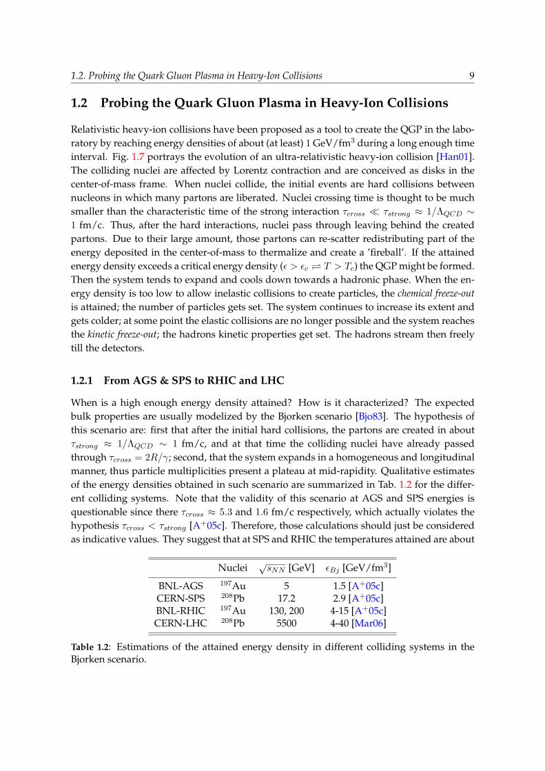
manner, thus particle multiplicities present a plateau at mid-rapidity. Qualitative estimates

of the energy densities obtained in such scenario are summarized in Tab. 1.2 for the differ-

ent colliding systems. Note that the validity of this scenario at AGS and SPS energies is

questionable since there τcross ≈ 5.3 and 1.6 fm/c respectively, which actually violates the

hypothesis τcross < τstrong [A+05c]. Therefore, those calculations should just be considered

as indicative values. They suggest that at SPS and RHIC the temperatures attained are about

Nuclei√sNN [GeV] ǫBj [GeV/fm3]

BNL-AGS 197Au 5 1.5 [A+05c]CERN-SPS 208Pb 17.2 2.9 [A+05c]BNL-RHIC 197Au 130, 200 4-15 [A+05c]CERN-LHC 208Pb 5500 4-40 [Mar06]

Table 1.2: Estimations of the attained energy density in different colliding systems in theBjorken scenario.


Figure 1.7: Sketch of a heavy-ion collision evolution. Snapshots of the time evolution (up-per figure) starting from instants before the collision (a), the formation of a QGP if a highenough energy density is attained (b), the later hadronization (c) and free-streaming of thehadrons towards the detectors (d) [Han01]. Then, (bottom figure) light-cone scheme of thesame collision evolution with more precise indication of the different phases of the QGPformation.

T < 2Tc while at LHC 3Tc could be reached. This is a crucial point we should bear in mind

to interpret QQ production in the sequential melting scenario.


1.2.2 Signatures: experimental observables

Experimentally we study the characteristics of the produced QCD medium analyzing the

kinematic and chemical properties of the particles emitted in the reaction. Practically only pi-

ons, kaons, (anti-) protons, electrons (positrons), muons, (anti-) neutrons and photons reach

the detector, and through analysis techniques the different particles produced in the colli-

sion can be identified. Those are the probes that serve us to infer the properties and phases

of the matter formed in the collisions. We can classify those probes as: global, initial and

final state observables.

Global observables

The global observables provide general information about the collision such as the centrality,

the reaction plane, the volume, the expansion velocity and the initial energy density [Mar06].

The measurement of the charged particle multiplicity, the transverse energy and the hadrons

kinematic properties (among others) permit those analysis. The reaction centrality can be

obtained from measurements of particle multiplicity and of the energy carried by participant

and spectator nucleons of the collision. On the other hand, studies of the transverse energy

as a function of centrality carry information about the ’fireball’ energy density, duration and

particles interaction.

Initial state observables

We consider as initial state observables those probes that should not be affected by the QGP

formation; those that behave in the same way in the presence of cold nuclear matter (p-A

collisions) or the QGP (A-B collisions). Electroweak bosons: high-pT γ, W± and Z0 are con-

ceived as initial state probes as they do not interact strongly [Mar06]. Weak bosons interest

and particularities will be further discussed in Sec. 2 and all through this manuscript we

focus on their production at LHC energies and measurement in the ALICE muon spectrom-

eter. With regard to photons, we should distinguish their different production processes. On

the one hand, there are direct photons, from which we can separate: the prompt photons,

issuing from initial hard collisions, and the thermal photons, emitted in secondary collisions

(in the thermal bath), either in the QGP phase or the hadronic phase. On the other hand,

there are the decay photons, mainly from π and η decays, that prevail quantitatively over

direct photons.

Final state observables

The final state observables are those that provide information on the hadronic and QGP

phases. Those are obtained from the hadron yields and kinematic properties. It would be

hard to list exhaustively all those probes, since they are many, but we could mention the

transverse momentum (pT ) distribution and the relative yield of the hadron species, the

flow, the high-pT particle correlations and the event fluctuations. For instance, due to chiral

restoration strange quarks are expected to be lighter at deconfinement, thus strange hadrons


are more easily formed; moreover, at deconfinement gluon density also contributes to in-

crease the strange hadrons yields.

Hard probes: As hard probes we refer to those that carry information on the first stages

of the collision: the equilibration process, the QGP and its transition [Mar06]. They are

produced in the early stages and their life is long enough to become sensitive to the QGP

formation before they fragment. As penetrating probes we can point out: high-pT particles

and jets, originating from high-pT partons fragmentation; resonances with short lifetime that

are produced and decay inside the fireball such as the ρ, ω and φ mesons; low-pT photons

that could indicate the fireball temperature8, and heavy quarks and quarkonia that could

probe the potential screening and will be discussed in more detail in Sec. 1.3. High-pT parti-

cles and jets may help to describe the partonic phase via studies of their possibly suppressed

invariant yield and their angular correlations as a function of the system energy and the re-

action plane. On the other hand, the mass and width of the short-lived resonances might be

modified by the chiral restoration at deconfinement.

1.2.3 Highlights from the SPS Heavy-Ion program

The CERN-SPS9 heavy-ion program concerned the NA44, NA45, NA49, NA50, NA52, NA60,

WA97 and WA98 experiments among others. They took data in p-p, p-A and A-B col-

lisions (A being a wide variety of nucleus from O, S and In, until Pb) from 40A GeV to

158A GeV (for Pb), where they studied among others the transverse energy, particles multi-

plicity, strangeness production, direct photons and charmonium production, and they con-

cluded that there was experimental evidence for the formation of a new state of matter as their

data could not be explained in terms of hadronic degrees of freedom alone [Gon01, HJ00].

Here we just comment on the most significant charmonia results, as they are of interest for

the present work.

J/ψ anomalous suppression

At SPS energies, J/ψ production in p-A collisions showed to be in agreement with expec-

tations from ’normal’ nuclear absorption. The NA50 experiment evidenced first an anoma-

lous suppression of J/ψ production in central Pb-Pb collisions at 158A GeV with respect to

p-A or S-U data [A+00a]. They identified J/ψ and ψ′ production through invariant mass

analysis of unlike-sign muon pairs and performed a comparison of the J/ψ and Drell-Yan

production as a function of the collision centrality. Where the centrality was determined

by measuring the transverse energy (ET ), the energy in the zero degree calorimeter (EZDC)

and the charged particle multiplicity; which allow to determine either the length traversed

by the charmonium state in nuclear matter L, or the number of nucleon participants in

8 The identification of the thermal photons should permit to probe the temperature of the bath in which theywere formed, and their invariant yield as a function of the reaction centrality should indicate the formation of ahottest state of matter in the most central collisions (there should be an excess of thermal photons if the QGP isformed).

9 SPS stands for Super Proton Synchrotron.


the reaction Npart. Later the NA60 experiment completed the studies with In-In data at

158A GeV [P+06, A+05f]. The results of the J/ψ over Drell-Yan ratio as a function of L

for different SPS experiments are plotted together in Fig. 1.8, where the red line represents

the expectations from nuclear matter absorption considering an absorption cross section of

4.18 ± 0.35 mb [A+05e]. Observe that in the central collisions (large L values) there is a

suppression with respect to cold nuclear effects expectations. This suppression attains a fac-

tor of 0.5 for the most central reactions, suggesting the formation of a deconfined medium.

However, we may note that it does not necessarily mean a suppression of direct J/ψ pro-

Figure 1.8: J/ψ over Drell-Yanproduction cross-section ratio as afunction of the length traversed bythe charmonium in nuclear mat-ter (L) for various colliding sys-tems [P+06].

duction, as a considerable amount of ψ′ and χc decay into J/ψ. As a matter of fact, at SPS

energies about 30-40% of the produced J/ψ come from higher resonances decays. The J/ψ

anomalous suppression could then indicate a suppression of the higher resonances. Various

models can reproduce the observed suppression either taking into account QGP formation

or considering hadronic interactions between the charmonium and the hadron gas. It is then

a general hope that either RHIC or LHC data could shed some light on this.

1.2.4 RHIC results in a nutshell

The RHIC10 collider has devoted its physics program to the study of nuclear matter un-

der extreme conditions of temperature and energy density. Four experiments have settled

there: PHENIX (Pioneering High Energy Nuclear Interaction eXperiment), STAR (Solenoidal

Tracker At RHIC), BRAHMS (Broad RAnge Hadron Magnetic Spectrometers experiment)

and PHOBOS (the name of the larger and innermost of Mars two moons). They have an-

alyzed p-p, d-Au, Cu-Cu and Au-Au collisions from 19A GeV to 200A GeV (in the center

10 RHIC stands for Relativistic Heavy Ion Collider.


of mass) since 2000 till today, obtaining a wide fan of experimental results. Comprehen-

sive data reviews were published in 2005 by all four experiments, where they all agreed to

claim that a strongly interacting matter was formed [A+05c, A+05b, A+05g, B+05]. Here I just

discuss on some aspects of two of those which I personally consider the most remarkable

observations: the jet quenching and the elliptic flow.

Elliptic flow

In reference [Oll92] it was shown that azimuthal anisotropies of particle emission with re-

spect to the reaction plane11 could be a signature of particles collective motion in heavy-ion

collisions, the collective flow. In nucleon-nucleon (N-N) collisions the azimuthal distribution

of the emitted particles is isotropic. If A-B collisions were an incoherent superposition of

N-N collisions, the azimuthal distribution of the particles would also be symmetric. But if

there were secondary interactions between the particles produced in the first N-N collisions,

the reaction zone anisotropy (see the nucleus overlap area in Fig. 1.9) could induce an az-

imuthal anisotropy on the emitted particles momenta.

Usually the azimuthal distributions are studied by analyzing the differential production

cross-sections in terms of a Fourier decomposition [PV98]

dN

pTdpTdydφ=

1

2π

dN

pTdpTdy

{1 +

∑

i=1

2vi cos[i(φ− ΨR)]}, (1.6)

vi = 〈cos[n(φ− ΨR)]〉 ,

ΨR being the reaction plane angle and vi the Fourier coefficients. The lowest order Fourier

terms are the so called direct flow (v1) and elliptic flow (v2). One of the first RHIC measure-

ments on this regard was the elliptic flow at STAR [A+05a]. Fig. 1.9 shows v2 RHIC re-

sults for different particle species. At small pT (pT <∼ 2-3 GeV/c) a good agreement with

hydrodynamic calculations is observed; the mass dependence is reproduced, the lighter

particles having a more important flow. This together with v2 dependence on centrality

and pT suggests that equilibrium is reached quickly, and indicate that at those energies a

perfect liquid (a strongly interacting liquid), more than an ideal-gas QGP could have been

formed [A+05c, A+05b, A+05g, B+05]. However, there is still some open questions to this

interpretation.

Jet quenching

Partons produced in initial hard collisions may traverse the QGP before they fragment. Due

to their color charge, they may interact with this dense matter loosing part of their energy.

Their fragmentation products would then be less energetic (than if no QGP is formed), lead-

ing to the so called jet quenching. Moreover, as in the parton model of LO-pQCD jets are

produced by pairs (with equal impulsion and direction but opposite sense in azimuth), if

11 The reaction plane is determined with respect to the impact parameter vector ~b and the nucleus initialimpulsion vector.


Figure 1.9: Sketch of a heavy-ion collision flow (left-figure). Elliptic flow v2 distribution as afunction of pT for various particle species at

√sNN = 200 GeV [A+05a] (right-figure).

one of those jets traverses a longer in-medium path their relative properties could be af-

fected. In the most extreme case they are produced near the bulk surface; one of the jets

escape without any modification, whereas the other crosses all the medium and could even

be fully screened. Fig. 1.10 presents a sketch of this situation.

Figure 1.10: Sketch of the back-to-back jets production in p-p collisionsand the in-medium influence in A-Bcollisions.

High-pT particles suppression: RHIC experiments have performed a detailed systematic

study of the nuclear modification factor for various particle species, colliding systems, en-

ergies and collision centralities. A snapshot of the obtained results is displayed in Fig. 1.11

[A+03, d’E04, A+05d]. We can observe in the left-hand figure the d-Au nuclear modification

factor (RdAu) as measured by PHENIX at√sNN = 200 GeV for charged hadrons and neu-

tral pions. An enhancement in the intermediate-pT region of about 2-8 GeV/c is evidenced

and commonly interpreted in terms of the Cronin-effect. It is thought that parton multiple

scattering in a cold nuclear medium produces a dispersion and widening of the partons pTdistribution. In addition, the nuclear modification factor of charged hadrons in the most

central 0-10% Au-Au collisions (RAuAu) is plotted, exhibiting a strong suppression of about

a factor 5 (RAuAu ∼ 0.2). Charged hadron suppression, which is also observed for the π0


observable at the same energy, is not noticed neither at lower energies (Fig. 1.11 upper-right

plot) nor for direct photon production (Fig. 1.11 bottom-right plot). The high-pT particle

suppression reveals then the effect of the jet quenching phenomena. RHIC results on the

nuclear modification factor suggest that a deconfined medium with a high gluon density

has been formed, causing a large parton energy loss [Mar06].

RdA(pT ) and RAA(pT ) (central collisions) for chargedhadrons and π0 at 200 GeV [A+03].

π0 RAA(pT ) at SPS, ISR & RHIC central colli-sions [d’E04].

RAA(pT ) for π0 and direct γ vs centrality [A+05d].

Figure 1.11: Compilation of the jet quenching phenomena results at RHIC. The nuclear mod-ification factor in d-Au collisions at 200 GeV for π0 and charged hadrons is compared tothe one of charged hadrons in Au-Au collisions at the same energy [A+03] (left figure). π0

RAA(pT ) for the most central heavy-ion collisions at SPS (CERN), ISR (CERN) and RHIC(BNL) energies [d’E04] (right-upper plot). Comparison of RAA for π0 and direct γ vs colli-sion centrality [A+05d] (right-bottom figure).

1.3 Heavy quarks and quarkonia

In this section we outline the different aspects influencing heavy quark and quarkonia pro-

duction. A qualitative estimate of their formation and decay times is needed to situate them

1.3. Heavy quarks and quarkonia 17

with respect to the collision evolution stages. Various models/mechanisms that might af-

fect their production in nucleon-nucleon, proton-nucleus and nucleus-nucleus collisions are

commented. It should be noticed that this is not an extensive review, just some points are

discussed.

1.3.1 Qualitative formation and decay times

It is commonly accepted that at LHC energies the main production mechanism of heavy

quark and quarkonia is gluon fusion gg −→ QQ. Gluons from the nucleus wave function

will form a QQ pre-resonance in a characteristic (hard) production time tp

tp(pT ≫ mQ) ∼ E

p2T

∼ 1

pT, tp(pT <∼mQ) ∼ 1

mQ, (1.7)

E being the pair energy. Thus, for pT ∼ mQ the production time of charm and beauty pre-

resonance pairs would be about

tp(pT ∼ mc) ∼ 0.15 fm/c , tp(pT ∼ mb) ∼ 0.05 fm/c .

The production time is then much smaller than 1 fm/c, and they are formed at a relative

distance 1/mQ ≪ 1 fm. Then the QQ pairs travel extremely close and to form a QQ reso-

nance they need to expand till the characteristic size of the resonance. It can be interpreted

as the time the pair takes to ’decide’ which of the possible QQ bound-states it will couple

to (one with mass m1 or one with m2). This formation time can be calculated by means

of [The94, KT99]

tf ≃ 2E

m22 −m2

1

. (1.8)

Thus the time a cc (bb) pair takes to ’decide’ to form a J/Ψ (Υ) rather than a Ψ′ (Υ′)

tf (J/Ψ, E) ≃ 2E

m(J/Ψ)2 −m(Ψ′)2, tf (Υ, E) ≃ 2E

m(Υ)2 −m(Υ′)2,

tf (J/Ψ, 10 GeV) ≃ 1.0 fm/c , tf (Υ, 10 GeV) ≃ 0.36 fm/c ,

tf (J/Ψ, 30 GeV) ≃ 3.0 fm/c , tf (Υ, 30 GeV) ≃ 1.1 fm/c .

The resonances formation times are thus much larger than the pre-resonances production

times. They increase with the particle momentum, ranging from a fraction of fm/c to about

3 fm/c.

Later, the QQ resonance being not a stable particle, it will decay with a characteristic proper

time inversely proportional to its width

td ≃1

Γ. (1.9)


The J/Ψ and Υ decay time would then be of about

td(J/Ψ) ≃ 1

93 keV= 2.1 · 103 fm/c , td(Υ) ≃ 1

54 keV= 3.7 · 103 fm/c .

Theoretical calculations estimate that at LHC energies the QGP might be formed in about

0.1 fm/c and might last ≥ 10 fm/c. The previous calculations suggest that: the QQ pre-

resonances are produced while the QGP is formed, but the QQ resonances are formed in

coexistence with the QGP, and may decay out of it.

1.3.2 Quarkonia production in nucleon-nucleon collisions

Color Evaporation Model

The Color Evaporation Model (CEM) is a statistical model that describes the probability of

charmonia states formation [G+95, AEGH96, AEGH97, GHE97]. It considers that the QQ

can either combine with light quarks to form light mesons or bind to form a quarkonia

resonance. Focusing on the charmonia production as an example, its hypothesis is that the

production cross-section of any charmonium state i (σi) is a fixed fraction of the cc cross-

section σccσi(

√s) = fi σcc(

√s) , (1.10)

fi being an energy-independent constant to be determined from data. As a consequence

it predicts that the production ratios of the different charmonium states must be energy-

independentσi(

√s)

σj(√s)

=fifj

= ctt . (1.11)

Although this model gives correct quantitative predictions as a function of√s, it does not

reproduce hidden charm cross-sections and can not describe the space-time evolution of

color neutralization [Sat06].

Color Singlet Model

The Color Singlet Model (CSM) [BBB+03, Lan05] uses the non-relativistic QCD formalism

(NRQCD) and suggests that the QQ pair is formed in the hard process with the proper

quantum numbers. For the J/Ψ formation this requires the emission of a gluon in the final-

state to form the color-singlet, g g −→ J/Ψ g. It underestimates the J/Ψ, Ψ′ and Υ states

hadroproduction cross-sections by one order of magnitude [BBB+03].

Color Octet Model

The Color Octet Model (COM) [BF95, CGMP95, BR96, Gei98, BFL01] uses the non-relativistic

QCD formalism (NRQCD) and proposes that the QQ pair combines with a soft collinear

gluon to form a color-singlet QQ − g state, as illustrated in Fig. 1.12. After a relaxation


time this state absorbs the gluon and turns into the physical state. It provides a description

of the formation process evolution and predicts a transverse polarization. However, the

predictions for J/ψ polarization at Tevatron have not been observed [A+00b].

Figure 1.12: Evolution of J/ψ produc-tion in the COM [Sat06].

1.3.3 Production in a p-A collisions: cold nuclear effects

When produced in a cold nuclear medium, in p-A collisions, quarkonium and heavy quark

production may be affected by the presence of the medium in any of their production stages.

In particular we discuss the nuclear shadowing and the nuclear absorption.

Nuclear shadowing

The parton distribution functions (PDFs) describe the probability distribution to find a par-

ton in a proton with a fraction x of the proton momentum. When dealing with nuclei, the

high parton density can affect them, resulting in a modification of the PDFs in nuclei. Heavy

quark and quarkonia production are mainly influenced by the gluon PDFs. So far model

predictions do not severely constrain gluon shadowing [FS99, EKS99, KTH01]. However,

PHENIX data favor moderate scenarios such as the EKS one [GdC07]. Nuclear modifica-

tions of the gluon distribution functions in a nucleus of A = 208 for different values of Q2

(RAg (x,Q2)) are presented in Fig. 1.13. The zone with small values of x (x < 10−2) shows a

Figure 1.13: Nuclear modification ofthe gluon distribution functions in anucleus of A = 208 for different val-ues ofQ2; from 2.25 GeV2 (solid line)to 10000 GeV2 (dashed line).

decrease of the PDF that is often called shadowing and could lead to a reduction of the pro-


duction rate. On the contrary, the x region of between 0.03 and 0.2 presents an increase of

the PDFs that is referred to as anti-shadowing and could enhance the production rate.

Nuclear absorption

Due to the elevate parton density in the nuclear medium, the QQ state might suffer col-

lisions with the surrounding nucleons either in the pre-resonance or the resonance stage.

This might resolve the pair, consequently reducing the quarkonia production rate, and aug-

menting the open heavy quark mesons production rate. The influence of nuclear absorption

should diminish with the collision center-of-mass energy, as the higher the energy of the

colliding system, the shorter their crossing time, and the smaller the effect [CF06].

1.3.4 Production in A-B collisions: hot nuclear effects

In a high energy density environment heavy quark and quarkonia produced in hard primary

collisions might be affected by the following effects.

Heavy quark energy loss

Heavy quarks crossing through a QGP might interact with the medium and loose energy

via various mechanisms. Collisional and radiative energy loss have attracted the theorists

attention, the latter being actually considered the most important effect at high-pT . As we

discuss in more detail those effects in Chapter 7, here we just comment that this may reduce

high-pT heavy quarks and quarkonia production rate.

Quarkonia dissociation

Several effects can influence quarkonia production by separating the heavy quarks in the

pre-resonance stage and impeding its formation. We can distinguish the comover collisions,

the color screening and the parton percolation.

Suppression by comover collisions: [BM88, GV90, GV97, CF05] It was proposed that mul-

tiple scattering of the quarkonia with the medium might provoke its dissociation resulting

in an effective suppression rate. This effect could occur either in a confined phase via the

comover hadrons or in a deconfined phase via the comover partons. An illustration of the

expected behavior is shown in Fig. 1.14 as a function of the medium energy density (ǫ). For

clarification purposes, in the plot was considered that there is little or no suppression in the

hadronic phase (ǫ < ǫ(Tc)), and that in the deconfined phase (for larger ǫ) the comover par-

tons density increase with ǫ; the quarkonia survival probability decreasing accordingly.

Suppression by color screening: Results of lQCD concerning the quarkonium binding

potential have already been discussed in Sec. 1.1.2 [Sat07, Sat06, KKS06]. They suggest that

if the QGP is formed, the color field between the heavy quarks gets modified by the presence


of the surrounding unbound color charges; the consequence being the sequential dissocia-

tion of the different quarkonium states as a function of the medium temperature or energy

density schematized in Fig. 1.15 for the J/ψ case (see Tab. 1.1 for the dissociation temper-

atures for the various quarkonia states). This scenario has also consequences on the mean

pT squared (〈p2T 〉), predicting its broadening with respect to the number of nucleon-nucleon

collisions (NABcoll ) as

〈p2T 〉AB = 〈p2

T 〉pp +NABcoll δ0 (1.12)

where δ0 describes the average ’kick’ the parton receives in each collision and is determined

with p-A data. Figs. 1.15 & 1.16 display the expected pattern of the J/ψ production probabil-

ity and 〈p2T 〉 behavior as a function of centrality. lQCD calculations are model-independent;

nevertheless nothing assures that the medium produced in heavy-ion collisions is the ther-

mal QCD matter studied by lQCD, and moreover the various evolution stages in the nuclear

collisions are not accounted for [Sat06].

Figure 1.14: J/ψ survival probability sup-pression by comover collisions [Sat06].

Figure 1.15: Sequential J/ψ survivalprobability suppression by color screen-ing [Sat06].

The Color Glass Condensate (CGC): [MV94, Mue99, McL03] The increase of A or√sNN

comes along with an augmentation of the parton density in the nucleus, the gluons becom-

ing predominant. At high enough A or√sNN the density is so large that there is an overlap

of the partons wave functions, and they percolate producing an interconnected network. If

the network resolution is sufficient, it could lead to quarkonia dissociation. The CGC allows

then to describe the initial conditions in heavy-ion collisions and accounts for the nuclear

effects (shadowing, saturation,...). However, to evaluate the effect of the parton resolution

scale on quarkonia or heavy quarks production it is model-dependent.

Quarkonia regeneration

In the hadronization phase quarkonia can be formed by the binding of heavy quarks from

different nucleon-nucleon collisions as well as from the same [GRB04, BKCS04, ABMRS03,

TM06]. If the heavy quarks abundance augments with respect to their thermal conditions,


statistical recombination favors quarkonia production with respect to light hadrons, result-

ing on quarkonia production enhancement. The quarkonia production cross-section increas-

ing faster with the energy than the light hadrons one, the probability of recombination aug-

ments with the energy density and the collision centrality. Moreover, in the regeneration

picture the mean 〈p2T 〉 is thought to be independent of the centrality since the heavy quarks

probably come from different collisions. Fig. 1.16 illustrates the probability of J/ψ produc-

tion as a function of the medium energy density ǫ compared to the opposite scenario of

sequential suppression.

J/

P

rod

uct

ion

Pro

bab

ilit

y!

1

Energy Density

(a)

exogamous regeneration

sequential suppression

Figure 1.16: Cartoon of J/ψ enhancement by recombination in front of the sequential dissoci-ation scenarios. Survival probability as a function of the energy density (a) and pT behavior(b) [Sat07].

1.3.5 Charmonium data interpretation: remarks

CERN-SPS and BNL-RHIC experiments have provided valuable data on charmonium and

open-charm production. The (in my opinion) most relevant SPS observations were com-

mented on Sec. 1.2.3 and RHIC data are recent and are still under discussion. Here we just

pretend to give the basic lines in a few words. SPS data observed an anomalous J/ψ sup-

pression seemingly in accord with different models, some accounting for the QGP formation

and some not. RHIC just provided fresh data of d-Au, Cu-Cu and Au-Au collisions. When

compared to SPS results is revealed an intriguing observation: a similar suppression is per-

ceived for both (in the J/ψ over Drell-Yan ratio vs ǫ) while the expected energy densities are

increased by a factor 1-5 for RHIC12 [A+05c]. One interpretation is that even though at RHIC

the J/ψ is further suppressed, the recombination of cc pairs in the hadronic phase cancels it

out. Another is the sequential melting of the quarkonium states; it suggests that direct J/ψ

are not suppressed neither at SPS nor at RHIC, and that the observed suppression is due

to the decrease of the feed-back contribution from higher resonances which are suppressed

earlier and are thought to be melt at both SPS and RHIC energies. The lQCD sequential

12 Note that the comparison is not experimentally trivial, since ǫ calculation is dependent of centrality deter-mination and is model-dependent. Each experiment measures differently the centrality, which could introducediscrepancies.


melting scenario has also consequences on the J/ψ mean pT squared (〈p2T 〉), predicting its

broadening with respect to the number of nucleon-nucleon collisions (NABcoll ). RHIC and SPS

data agree with such scenario, so it appears to be on the right track [Sat06]. Nevertheless

at the present time we can not discriminate any of the interpretations [GdC07]. More pre-

cise data on ψ′ production at SPS, on J/ψ production at RHIC energies, and the upcoming

LHC data where the lQCD predicted onset of J/ψ dissociation should be attained could be

conclusive.

1.3.6 Novel aspects of heavy flavor physics at LHC

The LHC collider will offer the possibility to produce head-on heavy-ion collisions (HIC) in-

creasing the center-of-mass energy by about a factor 30 with respect to RHIC [C+04, A+06].

The large amount of energy available in the center-of-mass will be accompanied by an aug-

mentation of the cc and bb pairs abundance [C+04, A+06]. Tab. 1.3 reports the expectations:

about 115 cc pairs and 5 bb pairs should be produced in the 0-5% Pb-Pb most central colli-

sions (see App. D and Tab. D.6 for the calculations). That is about 10 times more cc pairs and

100 times more bb pairs than at RHIC. Heavy flavor will allow to probe rather small values

SPS RHIC LHC LHCPb-Pb Cent Au-Au Cent p-p Pb-Pb Cent

N(cc) 0.2 10 0.2 115N(bb) – 0.05 0.007 5

Table 1.3: Expected number of cc and bb pairs produced in central heavy-ion and p-p colli-sions at SPS, RHIC and LHC energies.

of the gluon Bjorken-x (10−5,10−3); for such x values in HIC a large shadowing is expected

which could reduce heavy quark production with respect to binary scaling. Moreover, the

larger and denser is the matter traversed the larger the heavy quark energy loss. Only about

1% of those heavy quarks will end up in the formation of quarkonia bound states [MG07].

Due to the energies attained at LHC, in HIC the quarkonia nuclear absorption should dimin-

ish (the nuclei crossing time is smaller), the dissociation temperatures of J/ψ (and may be

even the Υ) in the sequential melting scenario should be reached, and the charmonia recom-

bination processes should also become relevant (the larger the abundance of heavy quarks

present in the medium). Bottomonia family which was not accessible at SPS and whose

studies at RHIC is under investigation will become a powerful signature at LHC. Whether

heavy quarks will thermalize or develop collective motion, and whether quarkonia will be

further suppressed or regenerated, are still open questions that LHC data might resolve.

The ALICE experiment at LHC has the capability to combine electronic, muonic and hadronic

channels to measure heavy flavor (hidden and open charm and beauty), being able to mea-

sure quarkonia down to pT ∼ 0 [Mar05, Ant07]. Note that ALICE is the unique LHC device

able to measure charmonia down to pT ∼ 0, and open charm down to pT ∼ 0.5 GeV/c in p-p


or p-Pb collisions (1 GeV/c in Pb-Pb collisions). The latter would be possible via the recon-

struction of the D0 −→ K− π+ decays in the central barrel; it will probably bring the most

precise measurement of the total charm production cross-section at LHC energies [A+06].

Novelties with the ALICE muon spectrometer

Single muon spectra and the correlated continuum invariant mass will allow to study beauty

production from pT ∼ 1 to 20 GeV/c [CGMV05, Cro05]. Beauty production cross-section,

cold nuclear effects, and beauty energy loss will be studied. An invariant mass resolution of

the order of 70 (100) MeV/c2 will permit to disentangle the resonances of the J/ψ (Υ) fam-

ily [C+04, A+06]. The resonances yields as a function of centrality and pT should permit to

probe the characteristics of the deconfined medium and might provide tools to discriminate

between the various suppression and coalescence models. The expected high J/ψ statis-

tics [SVR07] (about half a million during one Pb-Pb run and 3 millions in a p-p run) will

allow to measure it from pT ∼ 0 to 30 GeV/c, and investigate its polarization [A+07] and its

azimuthal asymmetry with respect to the reaction plane. Polarization measurements in p-p

collisions might help to discern between the different models proposed to describe quarko-

nia production mechanisms: the CSM predicts transverse polarization, the CEM no polar-

ization, and the COM (NRQCD) transverse polarization at large pT . Moreover, an increase of

quarkonium polarization in heavy-ion collisions is expected in case of QGP [IK03]. Another

important issue is that Υ(1S) and Υ(2S) will be measured from pT ∼ 0 to 8 GeV/c; the novel

observable of their relative yield NΥ(2S)/NΥ(1S) will then become accessible [Cro05, DC05].

The resonance ratios as a function of pT have been suggested to isolate the QGP effects as

in the ratio of NΨ′(2S)/NJ/Ψ(1S) or NΥ(2S)/NΥ(1S) the cold nuclear effects are washed out (at

least on the pT evolution). Recent calculations indicate that with the expected Υ(1S) and

Υ(2S) statistics their ratio would be sensitive to the QGP [DC05].

Chapter 2

Weak bosons in hadron-hadron collisions

The most exciting phrase to hear in science, the one that heralds

the most discoveries, is not ’Eureka’! (I found it!) but ’That’s

funny...

I. Asimov

From the point of view of nucleus-nucleus collisions, as electroweak bosons do not inter-

act strongly, they are usually considered as medium-blind references and they have been

proposed to tag jet energy in back-to-back produced jets (the γ-jet or the Z-jet probes).

The concept being to use the electroweak boson energy to estimate the energy loss of its

companion-jet1, as the bosons are not sensitive to the strong interaction and the jets suffer

from energy loss while traversing the QGP (see [CB05, MCC+07] and references therein).

But, is it enough to only rely on the fact that electroweak bosons do not interact strongly

to consider them as medium-blind references? We should remind that they interact electro-

magnetically, and by the way, we could interrogate about when are they produced and when

do they decay? Are these the bosons or their decay products which might cross the QGP?

So, could they be influenced by the QGP either electromagnetically or via their decay prod-

ucts? Besides, remember that weak bosons are considered as standard model benchmarks,

they are interesting probes by themselves already in p-p collisions. Here and all through this

thesis work we will discuss those issues. In this chapter we just draw the attention on those

that we consider the most important points, and mainly those related to heavy-ion physics

will be developed in this manuscript. To facilitate the comprehension of the whole, here

we first discuss the qualitative formation and decay time of weak bosons (Sec. 2.1), then we

briefly summarize the main motivations to study weak bosons at LHC energies (Sec. 2.2),

and finally we remind the basics of the electroweak theory and the particularities of the

weak interaction (Sec. 2.3).

2.1 Qualitative formation and decay times

Weak bosons are formed early due to their large mass: tp ∼ 1/M ∼ 10−3 fm/c. Their decay

time is by definition inversely proportional to their widths

td(Z0 → X) ≃ 1

2.495 GeV= 0.08 fm/c , td(W

± → X) ≃ 1

2.141 GeV= 0.09 fm/c .

1 It is based on the fact that in the parton model of pQCD, at LO jets are always produced by pairs, with equalmomenta and opposite sense of movement.

26 2. Weak bosons in hadron-hadron collisions

Therefore weak bosons are produced early, before the QGP is formed, and decay either be-

fore or within the QGP. As a result their decay products might be sensitive to the QGP. If

we focus on their leptonic decays, as leptons do not interact strongly, they should be hardly

influenced by the QGP (we will discuss this in more detail in Sec. 7.3). However, if we con-

centrate on Z beauty decays, which branching ratio is of about 15% [Y+06], b-quarks should

be sensitive to the QGP, and so the Z invariant mass in this channel (see more details in

Sec. 7.5.1).

2.2 Why should we study weak bosons at LHC?

Weak bosons properties have been studied at LEP (CERN), SLC (SLAC) and Tevatron (FNAL)

colliders in pp and e+e− collisions [Y+06]. At the LHC, large energy will be available in the

center-of-mass, enabling the possibility to produce W and Z bosons in p-p and in nucleus-

nucleus (A-A) collisions.

In the lowest order approximation, W and Z bosons are produced by the quark (q) - anti-

quark (q) annihilation process:

q + q′ → W± ; q + q → Z .

These subprocesses are characterized by the scale Q2 = M2 and the Bjorken-x values, which

can be determined by x1,2 ∼ M√se±y [TCSG05, CS05], whereM is the mass of the weak boson,√

s is the center-of-mass energy of the nucleon-nucleon collision, and y is the rapidity.

Their measurements at LHC will provide important information:

– These subprocesses are considered as Standard Model benchmarks. Their production

cross-sections are ’known’ with a precision dependent on the parton distribution func-

tions (PDFs) uncertainties. Therefore, they have been suggested as ’standard-candles’

for luminosity measurements, and to improve the evaluation of the detector perfor-

mances [TCSG05, CS05].

– In proton-proton (p-p) collisions, they will be sensitive to the quark PDFs at high Q2

(Q = MW/Z).

– In proton-nucleus (p-A) collisions, quark nuclear modification effects will become ac-

cessible at the same scale.

– Since weak bosons are probes produced in hard primary collisions and if we con-

centrate in their leptonic decay they do not interact strongly with the surrounding

medium created in the collision, they will allow binary scaling cross-checks in A-A

collisions.

– They could then be used as a reference for observing medium induced effects on other

probes, like the suppression of high transverse momentum (pT ) muons from charm

2.3. Basics of the electroweak theory 27

and beauty, or the jet quenching phenomena in the Z-jet observable2.

W and Z bosons can be measured via their leptonic decay. The decay W+ → l+ νl(W− → l− νl) has a branching ratio of 10.7 %, and the decay Z → l+ l− has a branching

ratio of 3.37 % [Y+06]. All through this thesis work we will bring our efforts to discuss weak

boson production at LHC energies, their measurement in the ALICE muon spectrometer,

and their utility to study heavy-ion collisions (in particular to investigate the QGP forma-

tion in them).

2.3 Basics of the electroweak theory

2.3.1 Historical outline

About 1968 Sheldon Glashow, Steven Weinberg, and Abdus Salam formulated a unified

theory of electromagnetism and weak interactions, the electroweak theory (label SU(2) ×U(1)), for which they shared the 1979 Nobel Prize in physics [Nob]. The application of the

gauge principle to the weak theory (label SU(2)) requires three mass-less spin-1 bosons.

The electroweak theory postulates then the existence of four mass-less gauge spin-1 bosons:

a triplet W+, W−, W0 plus a neutral single particle V0. The Standard Model predicts the

existence of at least one heavy spin-0 boson called the Higgs boson, in which relies the mass-

giving mechanism. Such mechanism can break the symmetry of the postulated triplet to give

the massive W+ and W−, the massive Z0, and the mass-less photon (γ). The electroweak

theory has three parameters: the Fermi coupling constantGF /(ℏc)3 = 1.166·10−5 GeV−2, the

electromagnetic coupling constant e, α = e2/ℏc = 1/137, and the Weinberg angle θW which

describes the mixing of the gauge fields to make the four observable bosons, sin2 θW ≃ 0.23.

Carlo Rubbia and Simon van der Meer were awarded with the Nobel Prize in physics on 1984 for the discovery

of the W and Z [Nob]. On the one hand, on 1972 Simon van der Meer published a report entitled ’Stochastic

damping of betatron oscillations in the ISR’ [dM72]. He is the architect of the ’beam cooling’ techniques which

permitted to make intense antiproton beams feasible and allowed the discovery of the W and Z. The firsts tests

of this technique were carried out at ISR (CERN) on 1974, and an small storage ring was rapidly converted on

1976-77. On the other hand, on 1973, the huge Gargamelle bubble chamber at CERN photographed the tracks of

a few electrons suddenly starting to move, seemingly of their own accord. It presented an evidence of the weak

neutral currents, showing that the electroweak theory was on the right track. But the discovery of the W and

Z had to wait till 1983, when thanks to the ’beam cooling’ techniques the SPS collider was able to provide high

enough luminosity beams. At that time the experiments UA1 (led by Carlos Rubbia) and UA2 (led by Pierre

Darriulat) measured unambiguous signals of W bosons (on January 1983) [A+83a, B+83b] and Z bosons (on

May 1983) [A+83b, B+83a].

2 Nevertheless, remark that the production cross-section of this process is relatively small. In Sec. 5.1.1 we willdiscuss the production cross-sections, and we will observe that the NLO corrections to weak boson productionaccount only for about 13% [FM04].


2.3.2 Introduction to the electroweak theoretical formalism

The electromagnetic interaction is described by a U(1)em symmetry with coupling constant

e, where the current is:

e jemµ = e Ψ γµQf Ψ, (2.1)

Ψ is the fermion wave-function and Qf its charge (Q = +1 for the electron). The vertex of

the interaction is then of the form:

− i eQf γµ. (2.2)

On the other hand, the weak interaction is described by a SU(2)L symmetry with cou-

pling constant g, where the charged and the neutral currents can be respectively written

as [HM84]:

j±µ = χL γµ τ± χL, j3µ = χL γµ1

2τ3 χL, (2.3)

χL are the spinor doublets, the subscript L denotes the left-handed spinors and records the

vector axial nature of the currents, and τ± = 12(τ1 ± iτ2) being τi are the Pauli matrices. The

weak vertexes are then of the form:

− ig√2γµ

1

2(1 − γ5), −i g

cos θWγµ

1

2(cfV − cfAγ

5), (2.4)

for the charged and neutral currents respectively, and where

cfV = T 3f − 2 sin2 θW Qf , cfA = T 3

f , (2.5)

with T 3 as the third component of the fermion weak isospin charge: T 3 =∫j30(x)d3x.

Tab. 2.1 presents the fermions charge and the third component of their weak isospin charge

as a function of their chirality state. Observe that the weak isospin component is zero for

right-handed fermions. Remark that the chirality operator γ5 of eq. 2.4 ensures that right-

Fermion Qf (T 3f )L (T 3

f )R

u, c, t +23 +1

2 0d, s, b −1

3 −12 0

νl 0 +12 -

l− −1 −12 0

Table 2.1: Values of the electric charge and the third component of the weak isospin for left-handed and right-handed fermions [HM84].

handed neutrinos do not participate on the weak interaction. As a matter of fact, there

is no experimental evidence of their existence. One may also notice, by a comparison of

the vertex factors for the electromagnetic and the weak interactions (eqs. 2.2 and 2.4), that

while the first interaction has a pure vectorial coupling (vertex as γµ), the latter contains


vector and axial vector parts (vertex as γµ (1 − γ5)). This difference explains that while the

weak interaction violates parity (P ), the electromagnetic interaction does not 3 . Eq. 2.3 also

makes evident the pure nature of the vector-axial (V-A) coupling for the case of the charged

weak currents, i.e. for W± couplings that are ’maximally’ mixed (vertex as γµ (1 − γ5)); in

contrast to the non-pure V-A nature of the neutral weak current, i.e. for the Z0 coupling

(vertex as γµ (cfV − cfAγ5)). That means that W± only couple with left-handed fermions (and

right-handed anti-fermions), while the Z0 coupling has also right-handed fermionic (and

left-handed anti-fermionic) components.

Finally, the electroweak theory proposed by Glashow, Weinberg and Salam is able to de-

scribe both together on a SU(2)L ⊗ U(1)Y symmetry. According to the theory the electro-

magnetic interaction ’sits across’ the weak interaction and the weak hypercharge. The weak

hypercharge (Y ) is defined by:

Q = T 3 +Y

2, (2.6)

and is described by a U(1)Y symmetry with coupling constant g′, so that the weak hyper-

charge current is [HM84]

jYµ = Ψ γµ Y Ψ. (2.7)

The currents can then be characterized by:

jemµ = j3µ +1

2jYµ , (2.8)

jNCµ = j3µ − sin2 θW jemµ , (2.9)

where NC stands for neutral current. By imposing the consistency of those equations, one

obtains the relationship between the coupling constants

e = g sin θW = g′ cos θW . (2.10)

2.3.3 Particularities of the weak interaction

Here we highlight some particularities of the weak interaction that will be useful for the

comprehension of the rest of the manuscript.

Feynman diagrams for the weak vertexes

The Feynman diagrams of W and Z vertexes are presented in Fig. 2.1 and Fig. 2.2 together

with the rules for the vertex construction. It is important to note that the weak interaction do

not mix the lepton generations but do connect the quark generations. The W vertex connects

two different fermions, either quarks or leptons. The electric charge, the lepton generation

3 The parity and charge conjugation transformations deal with space inversion ( ~r → −~r ) and charge particleconjugation (particle ⇋ antiparticle) respectively. Their respective conserved quantities are the parity and thecharge conjugation quantum numbers. Thus CP violation is interpreted as a different physical behavior ofparticles and antiparticles, matter and antimatter.


Figure 2.1: Feynman diagram for the Wf1f2 vertex with the rules for vertex construction[Wil05]. Where f stands for fermions, either quarks or leptons.

number, the quark number and color are conserved on the W vertex while the quark flavor

is not. In contrast, the Z vertex connects two identical fermions, or a fermion with an anti-

Figure 2.2: Feynman diagram for the Zf1f2 vertex with the rules for vertex construction[Wil05]. Where f stands for fermions, either quarks or leptons.

fermion , and on that case besides the conservation rules of the W vertex, the quark flavor is

conserved. So, the Z is attached to a fermion current in which the fermion does not change.

In addition, we should highlight that W bosons only couple with left-handed fermions

and right-handed anti-fermions.

Quark mixing on charged weak couplings

Cabibbo first explained the coupling of the quark generations considering just two genera-

tions of quarks. He assumed that the charged weak current couples ’rotated’ quark states

and not the quark mass eigenstates . On that case the charged weak current could be written

as [HM84]:

jµ =(u c

) γµ(1 − γ5)

2U

(d

s

)with U =

(cos θC sin θC− sin θC cos θC

), (2.11)

where U is the rotation matrix and θC the Cabibbo angle, the unique parameter that is de-

termined by means of experiments to be θC = 13.1◦ [Gri04].

Later, Cabibbo-Kobayashi-Maskawa (CKM) generalized the rotation matrix for the case of

three quark generations. Thus in the standard electroweak model the left-handed fermion


fields Ψi =

(νil−i

)and

(uid′i

)of the ith fermion family transform as doublets under SU(2),

where d′i ≡∑

j Uijdj and U is the CKM mixing matrix

U =

|Uud| = 0.9738 |Uus| = 0.2272 |Uub| = 3.96 · 10−3

|Ucd| = 0.2271 |Ucs| = 0.9722 |Ucb| = 42.2 · 10−3

|Utd| = 8.1 · 10−3 |Uts| = 41.6 · 10−3 |Utb| = 0.99910

, (2.12)

which can be parameterized by three mixing angles and a CP-violating phase [Y+06].

Parity violation

The parity operator (P ) deals with space inversion ( ~r → −~r ) and has two eigenvalues: ±1. Pseudo-scalars

( Ψ γ5 Ψ ) and vectors ( Ψ γµ Ψ) have associated a parity −1 and scalars ( Ψ Ψ ) and axial vectors ( Ψ γµ γ5 Ψ )

+1. On a two dimensional plane, to perform a parity transformation is equivalent to apply a 180◦ rotation, that

is why it is usually referred to as mirror symmetry.

The particle helicity (h) characterizes the particle spin (~S) projection on the momentum di-

rection (~p), that is

h =~S · ~p|~p| . (2.13)

As the parity of spin and momentum are opposite: P (~S) = ~S, P (~p) = −~p, the helicity

changes sign under parity P (h) = −h. In the extreme relativistic limit or in the case of

mass-less particles, the chirality operator (γ5) is equal to the helicity operator [HM84]. The

chirality right-handed and left-handed projection operators are:

PR ≡ 1

2(1 + γ5), PL ≡ 1

2(1 − γ5). (2.14)

Then, for example, the left-handed electron 12(1 − γ5)u = uL corresponds to an electron

of negative helicity. So in the ultra-relativistic limit negative helicity corresponds to left

chirality, and positive helicity to right chirality. As the weak interaction just act with left-

handed neutrinos and right-handed antineutrinos, it violates parity4.

Parity violation on charged weak couplings was first suggested by Lee and Yang on 1956.

One year later the experience proposed by Lee and Yang was achieved by Wu [WAH+57],

and Lee and Yang were awarded with the Nobel Prize of physics that year [Nob]. In the Wu

experiment represented in Fig. 2.3, the nuclear spins of a sample of 60Co were aligned by

an external magnetic field and it was observed an asymmetry on the emission direction of

the electrons. The electrons were preferably emitted on the opposite direction to the Cobalt

nuclear spin, which testified the parity violation effect. One can understand that observing

that on this experiment angular momentum conservation on the Cobalt decay imposes that

J(e− + νe) = 1. As the antineutrino is right-handed, in order to keep J = 1 the antineutrino

4 For instance, if one applies parity transformation to a left-handed neutrino, one should reverse the sense ofthe spin rotation, then one gets a right-handed neutrino. But right-handed neutrinos do not exist, thus the paritytransformation is violated.


Scheme of Wu experience: 60Co → 60Ni +e−L + νR .Cartoon of P violation.

Figure 2.3: Sketch to describe the 60Co experiment; where the thin lines represent the move-ment (momentum) direction, and the thick lines represent the helicity.

is preferably emitted on the direction of the Cobalt nuclear spin, thus the electron tends to

be emitted on the opposite direction.

Part II

Experimental apparatus

Chapter 3

The Experiment

A spider conducts operations that resemble those of a weaver, and

a bee puts to shame many an architect in the construction of her

cells. But what distinguishes the worst architect from the best of

bees is this, that the architect raises his structure in imagination

before he erects it in reality.

K. Marx

Abstract

This chapter is an introduction to the experimental setup. The LHC collider and the ALICE

experiment are briefly described. Special attention is payed to the ALICE muon spectrometer.

3.1 The Large Hadron Collider

The Large Hadron Collider (LHC) is a particle accelerator, which is being installed in a tun-

nel of 27 km in circumference, buried 50-175 m below ground. It is located between the Jura

mountain range, in France, and the Lake of Geneva, in Switzerland. The tunnel was built in the

1980s for the previous big accelerator, the Large Electron Positron collider (LEP) . The LEP collider was origi-

nally foreseen to produce electron-positron collisions at energies up to 200 GeV, and achieved a collision energy

of 209 GeV in its last year of running, in 2000.

The LHC will produce head-on collisions between two beams of particles, either protons or

heavy ions. The beams will be produced and pre-accelerated in CERN’s chain of accelerators

(see Fig. 3.1), and then injected into the LHC. It will be the first accelerator able to generate

proton-proton collisions at√sNN = 14 TeV, that is a factor 7 with respect to TEVATRON

energies, and lead-lead collisions at√sNN = 5.5 TeV, a factor 30 with respect to the RHIC

collider. The LHC nominal running conditions in the ALICE experiment interaction point

are summarized in Tab. 3.1. This new energy domain will open new insights in particle and

nuclear physics.

3.1.1 The beam travel road

In the LHC accelerator, particles circulate in a vacuum tube, are kept in circular orbits using

dipole magnets, are focused by means of quadrupole magnets, and are accelerated at LHC

cavities with electromagnetic resonators. In Fig. 3.2 can be seen some details of the LHC ring

and of the cryodipoles. The maximum energy of the collisions is determined by the dipole

36 3. The Experiment

p-p Pb-Pb Ar-Ar p-Pb√sNN [TeV] 14 5.5 6.3 8.8

〈L〉 [cm−2s−1] 3 · 1030 5 · 1026 1029 1029

Rate [s−1] 2 · 105 4 · 103 3 · 105 2 · 105

Runtime [s] 107 106 106 106

σgeom [b] 0.07 7.7 2.7 1.9

Table 3.1: LHC nominal running conditions at interaction point 2, in the ALICE experiment.

magnet parameters and the collider circumference, in particular by their magnetic rigidity

(Bρ). The momentum P of the beam particles is given by

P = q Bρ −→ P

A=Z

AeBρ .

Since the maximum energy delivered by the LHC for proton beam is 7 TeV, the correspond-

ing maximum energy for lead beams is 2.7A TeV (Z/A ∼ 0.4).

The travel done by proton and lead ion beams (as an example of heavy ion beam) from their

production point till their interaction point following is outlined in Fig. 3.1.

Proton beam The proton beam travel [Sch99] begins at the Linac2. Orbiting electrons are

stripped off from hydrogen atoms. The protons are sent at an energy of 50 MeV from the

Linac2 to the Proton Synchrotron Booster (PSB), and accelerated to 1.4 GeV. Then the beam

is fed to the Proton Synchrotron (PS) and accelerated to 25 GeV. Later it is injected into the

Super Proton Synchrotron (SPS), where it is accelerated to 450 GeV. Afterwards the protons

are transferred to the LHC where they are accelerated to their nominal 7 TeV energy.

Lead ion beam The lead ions are produced by the Electron Cyclotron Resonance sources

(ECR) [Mar06] and later transferred to the Linac3. The ERC is a plasma device that permits

to generate multi-charged ion states with the help of heat, a magnetic field and microwaves.

A sample of different charge states with a maximum of Pb27+ are produced. These ions are

selected, accelerated to 4.2 MeV/nucleon (energy per nucleon) and passed through a carbon

foil, which strips most of them to Pb54+. The Pb54+ beam is accumulated and accelerated

to 72 MeV/nucleon in the Low Energy Ion Ring (LEIR). It is sent to the PS, which accelerates

it to 5.9 GeV/nucleon, passes it through a second foil (which fully strips it to Pb82+) and

transfers it to the SPS. Finally the SPS accelerates it to 177 GeV/nucleon and injects it to the

LHC, where it is accelerated to the nominal 2.76 TeV/nucleon energy [Sch99, B+04].

3.2 The ALICE Detector

A Large Ion Collider Experiment, i.e. ALICE [C+04, A+06], was designed for the study of

heavy ion collisions [Ant07]. The experiment will allow to investigate a wide fan of observ-

3.2. The ALICE Detector 37

pLINAC2

Gran Sasso

North Area

LINAC3Ions

East Area

TI2TI8

TT41TT40

CTF3

TT2

TT10

TT60

p

e–

ALICE

ATLAS

LHCb

CMS

CNGS

neutrinos

neutrons

pp

SPS1976 (7 km)

ISOLDE1989

BOOSTER1972 (157 m)

AD1999 (182 m)

Leir2005 (78 m)

2006

n-ToF2001

LHC2007 (27 km)

PS1959 (628 m)

4 p (proton) 4 ion 4 neutrons 4 p (antiproton) 4 4 proton/antiproton conversion 4 neutrinos 4 electron–

LEIR Low Energy Ion Ring LINAC LINear ACcelerator n-ToF Neutrons Time Of Flight

AD Antiproton Decelerator CTF3 Clic Test Facility CNGS Cern Neutrinos to Gran Sasso ISOLDE Isotope Separator OnLine DEvice

LHC Large Hadron Collider SPS Super Proton Synchrotron PS Proton Synchrotron

CERN Accelerator Complex

Figure 3.1: CERN Accelarator Complex.


Schema of the LHC ring The LHC cryodipole

Figure 3.2: Details of LHC collider.

ables from very low (∼ 100 MeV/c) up to fairly high (∼ 100 GeV/c) transverse momenta,

pT , in a center-of-mass energy domain not explored up to now. It will be able to track and

identify particles in this pT interval and to perform these tasks in a large particle multiplicity

environment (up to 8000 particles per unit of rapidity at mid-rapidity1).

Figure 3.3: ALICE detector layout.

1 The experiment was designed about 10 years ago in order to work in an expected harsh environment of 8000particles per unit of rapidity at mid-rapidity. Nowadays RHIC data suggest to update the predictions reducingthis value by a factor of 4, which assures that ALICE can perfectly cope with the expected particle multiplicities.


Figure 3.4: ALICE longitudinal and transversal sections, including EMCAL. In PHOS and HMPIDcoverage regions neither TRD nor TOF detectors are color filled.

The ALICE experiment consists of some detectors for measuring global observables (defined

as global detectors), a central barrel and a muon spectrometer. The central barrel covers a

pseudo-rapidity range of |η| ≤ 0.9, is flooded by a magnetic fieldB ≤ 0.5 T generated by a

large solenoidal magnet (L3), and is in charge of tracking and identifying charged particles

and photons. From the vertex region to the outer part it is composed by a vertex detec-

tor, the Inner Tracking System (ITS), a large Time Projection Chamber (TPC), a Transition

Radiation Detector (TRD) for electron identification, and a Time Of Flight detector (TOF)

to identify protons, kaons and pions, all of them with full azimuth acceptance. It disposes

also of a High Momentum Particle Identification (HMPID) detector to extend the transverse

momenta coverage of particle identification, and a Photon Spectrometer (PHOS) to identify

photons, both with reduced azimuthal acceptance. The muon spectrometer covers a pseudo-

rapidity range of −4.0 < η < −2.5, has its proper magnetic field ofB ≤ 0.7 T provided by

a dipole magnet, and is responsible of muon tracking and reconstruction. For this purpose

it consists, from the interaction vertex forwards, of a front absorber, five tracking stations,

an muon filter and two trigger stations. In addition, the ALICE global detectors are the For-

ward Multiplicity Detector (FMD), the Photon Multiplicity Detector (PMD), the V0 and the

T0, that take care of event particle multiplicity and beam luminosity measurement, and the

Zero Degree Calorimeter (ZDC) in charge of event centrality evaluation. The experiment

is completed by an array of scintillators for triggering on cosmic rays (ACORDE) and an

ElectroMagnetic CALorimeter (EMCAL)2. The detector layout can be seen in Fig. 3.3, and

longitudinal and transversal sections can be observed in Fig. 3.4.

2 ALICE EMCAL will cover |η| < 0.7 and π/3 < φ < π but will not be installed the first year of data-taking.


3.2.1 Global detectors

As global detectors we considered the FMD, the PMD, the V0, the T0 and the ZDC. In partic-

ular we refer to the ALICE forward detectors as: the FMD, the V0 and the T0. Fig. 3.5 shows

their position with respect to the ITS [C+04, ALI04]. Further details of those detectors can be

observed on Fig. 3.6.

Figure 3.5: Forward detectors location schema. From left to right up to ITS: T0, V0, FMD, ITS.

FMD: Forward Multiplicity Detector

The Forward Multiplicity Detector, FMD, consists of five rings of silicon strip detectors

whose dimensions are presented in Tab. 3.2. It is in charge of evaluating the charged par-

ticle multiplicity in the pseudo-rapidity range −3.4 < η < −1.7 and 1.7 < η < 5.1, and it

will also permit to determine the reaction plane event-by-event. Together, the ITS and the

FMD will provide an early charged particle multiplicity measurement for −3.4 < η < 5.1 in

all colliding systems.

In order to reconstruct particle multiplicity with the FMD two approaches can be considered. The Poisson ap-

proach assumes that on average each channel will be traversed by about one charged particle per central event3.

3 The extreme approach of 8000 particles per unit of rapidity at mid-rapidity drives to an evaluation of lessthan 3 charged particles per strip for all channels, including background.

V0 scheme. T0 prototype. FMD scheme.

Figure 3.6: Details of V0, T0 and FMD.


Then multiplicity information can be obtained by comparing the number of occupied and empty channels. That

is counting the number of empty channels, and evaluating the charged particle multiplicity by statistics. The

other approach, that will be more probably used, is to derive charged particle multiplicity from the measure-

ment of the deposited energy on each strip. This approach supposes that each particle deposes (on average) the

same amount of energy (minimum ionizing particles, MIPs).

Ring z (cm) Rin (cm) Rout (cm) η coverage

Si1 outer −75.2 15.4 28.4 −2.29 < η < − 1.70Si1 inner −62.8 4.2 17.2 −3.40 < η < − 2.01Si2 outer 75.2 15.4 28.4 1.70 < η < 2.29Si2 inner 83.4 4.2 17.2 2.28 < η < 3.68

Si3 340.0 4.2 17.2 3.68 < η < 5.09

Table 3.2: FMD detector dimensions.

V0

The V0 detector is involved on fast trigger and centrality determination tasks. It is made

of two arrays of scintillator counters, labeled V0A and V0C, that are segmented into four

rings and eight sectors (sectors of 45◦). The scheme of one array can be observed in Fig. 3.6.

The V0A is located at z = 340 cm, and the V0C at z = −90 cm, in front of the muon absorber.

The rings angular coverage is presented on Tab. 3.3.

V0A V0CRing ηmax/ηmin θmin/θmax ηmax/ηmin (π − θ)min/(π − θ)max

1 5.1/4.5 0.7/1.3 −3.7/− 3.2 2.8/4.72 4.5/3.9 1.3/2.3 −3.2/− 2.7 4.7/7.73 3.9/3.4 2.3/3.8 −2.7/− 2.2 7.7/12.54 3.4/2.8 3.8/6.9 −2.2/− 1.7 12.5/20.1

Table 3.3: η coverage and angular acceptance (in deg) of the rings for V0A and V0C.

Each counter consists of scintillator material with embedded WaveLength Shifting (WLS) optical fibers to collect

the produced light. These fibers absorb predominantly the blue light and reemit green light. The light is then

transmitted through a clear fiber to a photo-multiplier tube (PMT) located at 3 − 5 m from the detectors. Each

individual counter has a time resolution better than 1 ns and provides time-of-flight and signal charge informa-

tion. It characterizes the V0 a fast detector. The V0 will provide a fast trigger signal and it

will permit to validate the muon trigger signal by rejecting beam-gas interactions4. Par-

ticularly, as trigger signals it will provide a minimum bias trigger and two centrality triggers

4 Beam-gas interactions can be identified by measuring the time-of-flight difference of V0A and V0C signals.


(on Pb-Pb collisions), as the T0 will. It will also serve as a centrality indicator, and it will

permit to control the beam luminosity.

T0

The T0 detector is made of two arrays of Cherenkov counters with 12 individual counters

per array. The right array, T0C, is located at z = −70 cm (muon spectrometer side) and

covers −2.9 < η < −3.3. The left array, T0A, is located farther from the interaction point,

at z = 350 cm, and covers 5 < η < 4.5. Each Cherenkov counter is based on a fine-mesh

photo-multiplier tube, 30 mm in diameter and 45 mm long, optically coupled to a quartz

radiator 30 mm in diameter and 30 mm thick. This detector has a time resolution of about

50 ps (individual counters have a time resolution of 37 ps), and is able to measure the vertex

position with a resolution of 1.3 cm. The T0 is in charge of:

– Provide a measurement of the collision time, a T0 signal that the TOF detector needs.;

– Generate a L0 trigger by means of a fast vertex position measurement. It helps to

discriminate against beam-gas interactions;

– Provide an early ’wake-up’ signal to the TRD, prior to L0 ;

– Measure particle multiplicity and generate three possible trigger signals : minimum

bias, and two centrality triggers (as the V0 will).

PMD: Photon Multiplicity Detector

The pre-shower Photon Multiplicity Detector, PMD, measures event-by-event photon mul-

tiplicity and spatial (η,ϕ) distribution of photons [C+04, ALI99c, ALI03]. It is located at

z = 360 cm and covers 2.3 ≤ η ≤ 3.5. Fig. 3.7 presents its structure. It consists of two iden-

Figure 3.7: Photon Multiplicity Detector structure. S.S. is the support plate for the lead con-verter plates.

tical planes of detectors with a 3X0 lead converter in between them. The detector is a gas


proportional counter with wire readout and the particularity of having a honeycomb struc-

ture and operating with a mixture of Ar/CO2 (70%/30%). The hexagonal cells have a cross

section of 0.22 cm2, and a depth of 0.5 cm. The detector plane situated on the interaction side

is used for vetoing charged particles and is labeled the veto, and the other detector plane is

called the pre-shower and gives both photons and charged hadrons signals. So the photon

signal can be disentangled.

ZDC: Zero Degree Calorimeter

The Zero Degree Calorimeter, ZDC, role is to measure the number of spectator nucleons

and hence to determine the centrality of the interaction [C+04, ALI99e]. When an inter-

action takes place, the spectator nucleons (the nucleons that do not interact) are ejected at

forward rapidities. The ZDC measures the number and energy of these spectator nucleons

in order to evaluate the number of participants and the event centrality.

The detector is composed by two hadronic calorimeters: the neutron calorimeter (ZN, that

measures the spectator neutrons), and the proton calorimeter (ZP, that measures the specta-

tor protons), and by an electromagnetic calorimeter (ZEM, that estimates the participating

nucleons). The hadronic calorimeters are placed at z = ±116 m and are made of a dense passive material and

quartz fibers (Cherenkov detectors) interspersed in the passive material. The spectator nucleons entering the

calorimeter generate showers which produce Cherenkov radiation that is detected by the quartz fibers. The ZN

is located between the two beam pipes, to profit that neutrons are not deflected by the LHC machine magnetic

field. In opposition, the ZP is placed externally to the outgoing beam pipe, on the side where the positive parti-

cles are deflected. Fig. 3.8 shows ZP and ZN position with respect to the LHC beam pipes, and Tab. 3.4 presents

ZN, ZP and ZEM characteristics. On the other hand, the two ZEMs are placed at z = 7 m, in the opposite side

ZN ZP ZEM

z (m) 116 116 7Dimensions (cm3) 7.04 × 7.04 × 100 12 × 22.4 × 150 7 × 7 × 21Absorber material Tungsten alloy Brass LeadFiber orientation 0◦ 0◦ 45◦

Filling ratio 1/22 1/65 1/11

Table 3.4: ZDC calorimeters dimensions and characteristics.

of the muon spectrometer, and covers 4.8 < η < 5.7. It evaluates the participating nucleons by measuring the

energy of the generated showers. The detector technique is the same that for the ZN and ZP, but it is made

of lead planes of 3 mm readout by sandwiched quartz fibers, which are oriented at 45◦ (where the peak of the

Cherenkov produced light is).

By comparing the energy measured by the ZEM, EZEM , and the energy of the spectator nu-

cleons EZDC = EZN +EZP , one is comparing the number of participants and the number of

spectator nucleons. Then, one can determine the centrality of the interaction. As an example,

Fig. 3.9 presents a plot where 10 centrality classes have been defined.


Location of the proton and neutron calorimeters. View of a neutron calorimeter.

Figure 3.8: Details of the ZDC.

Figure 3.9: Centrality classes determination from ZDC energy and ZEM energy, using fastsimulations.

3.2.2 Central Barrel

ITS: Inner Tracking System

The Inner Tracking System, ITS, is the innermost detector of ALICE and its main purpose

is to participate in tracking and to provide vertexing measurements to the experiment. It

consists of six cylindrical layers of silicon detectors and covers |η| ≤ 0.9 for all vertices

located within the length of the interaction diamond (± 1 σ, i.e. 10.6 cm along the beam

axis) [C+04, ALI99b]. It combines different silicon detector technologies in order to accom-

plish its design requirements regarding its acceptance coverage, the dE/dx measurement,

the desired spatial resolution, the need to minimize the amount of material in the active vol-

ume, the radiation levels attained at this area, and the readout rate. Thereby, the innermost


two layers are equipped with Silicon Pixel Detectors (SPD), the following two layers are

equipped with Silicon Drift Detectors (SDD) and the external two layers with double-sided

Silicon micro-Strip Detectors (SSD). ITS layout can be observed on Fig. 3.10, and Tab. 3.5

summarizes its dimensions and characteristics. We can point out that the first layer has a

wider pseudo-rapidity coverage |η| ≤ 1.98 to permit a continuity on the measurement

of charged particle multiplicity at higher rapidities (together with the FMD). On the other

hand, the four outermost layers will have analogue readout to allow dE/dx measurement

for particle identification. Basically, the ITS is able to:

– Localize the primary vertex with a resolution much better than 100 µm ;

– Reconstruct secondary vertices from decays of hyperons and D and B mesons;

– Improve the TPC measurements extending momentum coverage below 100 MeV

and ameliorating the (p, θ) resolution .

Figure 3.10: ITS layout.

Layer Type r (cm) ± z (cm) S.P. rϕ(µm)/z(µm)

1, 2 Pixel 3.9, 7.6 14.1 12/1003, 4 Drift 15.0, 23.9 22.2, 29.7 38/285, 6 Strip 37.8/38.4, 42.8/43.4 43.1, 48.9 20/830

Table 3.5: ITS detector dimensions and characteristics [C+04], where S.P. stands for spatialprecision.

TPC: Time Projection Chamber

The ALICE Time Projection Chamber, TPC, is the main tracking detector of the ALICE cen-

tral barrel [C+04, ALI00b]. It is in charge of tracking and determining charged particle mo-


menta with a good two-track separation, to enable particle identification and event vertex

position evaluation . It will be able to determine charged particles pT from 100 MeV/c (with

1%− 2% resolution) up to 100 GeV/c (with ∼ 5% resolution if ITS is also used). The harm of

using the TPC is its memory time, which limits the luminosity that the ALICE experiment

can afford.

The TPC is a cylindrical cage of 510 cm long (z position between ±255 cm), internal radius

of 84 cm and external radius of 246 cm. It covers |η| ≤ 0.9 (up to |η| ∼ 1.5 for tracks

with a small track length). Fig. 3.11 presents a scheme of the TPC layout. It is characterized

by having a central high-voltage electrode of 100 kV and two opposite axial potential degraders, providing a

highly uniform electrostatic field of 400 V cm−1 in the common gas volume, which is filled with 88 m3 of a

Ne/CO2 mixture (90%/10%). Those characteristics result on a maximum drift time of 88 µs which limit the

memory time of the TPC. The end-plates of the detector are equipped with multi-wire proportional chambers

Figure 3.11: TPC layout.

with cathode pad readout, structured in 18 trapezoidal sectors at each end-plate. Those sectors are radially seg-

mented into two chambers at radii 84.1, 132.1, 246.6 cm. The readout chambers pad sizes are of 4 × 7.5, 6 × 10

and 6×15 mm2. Those chambers are closed by a gating grid, located above the cathode wire grid, with alternate

wires connected together electrically. When there’s a L1 trigger (6.5 µs after the collision), the gates are opened

for the duration of the drift time. That means that the wires are held at the same potential, permitting the pass

of the electrons generated in the drift region into the amplification region. Otherwise the gate is closed, the grid

is biased by a bipolar field, preventing the electrons to enter the amplification region and stopping the ions cre-

ated by avalanche processes in the amplification region. The gates have then the mission to prevent TPC space

charge.


TRD: Transition Radiation Detector

The Transition Radiation Detector, TRD, covers |η| ≤ 0.9 and is situated between the TPC

and the TOF detectors, that is at a radius of (2.9, 3.7) m and |z| < 3.5 m [C+04, ALI01]. It is

composed by 18 sectors (as the TPC), and each sector is made of 6 layers and 5-fold segmen-

tation along the beam axis (that is a total of 18× 6× 5 = 540 modules). The module consists

of a radiator of 4.8 cm thickness and a multi-wire proportional chamber (MWPC) with cath-

ode pad readout. The chambers are filled with a gas mixture of Xe/CO2 (85%/15%), and

the typical pad size is of 6 − 7 cm2. The detector rϕ resolution is about 400 µm. The TRD

momentum resolution in standalone mode is:

∆P

P≈ 2.5% ⊕ 0.5(0.8)% · P (GeV/c) for

dNch

dη= 2000(8000)

The principle of the radiation detector comes from the fact that when a relativistic charged

particle traverse the boundary of two media of different dielectric constant, it produces tran-

sition radiation. It depends strongly on the relativistic γ factor, which makes it suitable for

particle discrimination. In particular, for the P range 1 − 100 GeV/c just the electrons pro-

duce transition radiation. Radiation that is in form of X-rays (energy in the keV range) and

has a peaking angle of the order of 1/γ relative to the particle’s path.

Schema of a TRD. Measured signal vs time for π and e.

Figure 3.12: Schema of a TRD module and of the measured signal vs time spectra for e and πwith and without the radiator.

Fig. 3.12 presents a sketch of a TRD module and a figure of the measured signal versus time for electrons and

pions. The electron signal with and without the presence of the radiator is plotted. The pion signal represent the

signal of a charged particle crossing the MWPC, where the peak in the first µs comes from the particles ionized

in the multiplication region. On the other hand, for the chosen gas mixture, when there’s transition radiation

produced the X-rays are absorbed at the beginning of the MWPC, so their signal reaches the pads on the latest

moments (with respect to the drift time). This characteristic makes possible the electron identification with the

TRD.


The TRD main functionality is to provide electron identification for P > 1 GeV/c by hav-

ing a good π rejection capability (π suppression of 10−2)5. As it is a fast tracker, it can

serve as trigger for high pT electrons (L1 trigger for single tracks of pT > 3 GeV/c), and

for electron pairs (online PID), and it helps to improve the hadron P measurement and

identification.

TOF: Time Of Flight

The Time Of Flight detector, TOF, covers |η| ≤ 0.9 and takes care of particle identification

in the intermediate momentum range (0.2 < P < 2.5 GeV/c) [C+04, ALI02b, ALI02a]. To-

gether with the ITS and the TPC (for vertex reconstruction and dE/dx measurement at low

P ), they will permit event-by-event identification of pions, kaons and protons. It is com-

posed by 18 sectors (in ϕ) of 5 segments each (in z) of Multi-gap Resistive Plate Chambers

(MRPC) rϕ oriented. It is localized at a radius of 3.70 < r < 3.99 m, has a total length

of 7.45 m, and its chambers pad size is of 3.5 × 2.5 cm2. The TOF is characterized by a

time resolution better of 40 ps, with permits to identify π, K for 0.2 − 2.5 GeV/c, p for

0.4 − 4.5 GeV/c, and e for 0.1 − 0.5 GeV/c.

Figure 3.13: Mass separation as a function of momentum with the TOF detector, for 200HIJING central PbPb events and with a simulated overall TOF time resolution of 80 ps. Theright plots present the mass distributions for 0.5 < P < 4.2 GeV/c in linear and logarithmicscales [A+06].

The identification of the hadrons resides in their different time of flight vs P behavior. The

ITS-TPC reconstructed tracks are projected into the TOF, and for the matched particles the

travel length (l) is calculated from the track momentum (P ). The time of flight (t) allows to

evaluate the particle mass as: m = P√t2/(l2 − 1) [ALI02b]. Particles are then entered in a P

versus m plot, as the one of Fig. 3.13, which permits to identify them.

5 That means that for each 100 hadrons, just 1 would be labeled as an electron by the TRD.


HMPID: High Momentum Particle IDentification

The High Momentum Particle IDentification, HMPID, is one of the outer detectors of ALICE

[C+04, ALI98]. It is located at a radius of 5 m and its azimuthal and pseudo-rapidity cover-

age are of ∆ϕ = 57.61◦ and |η| ≤ 0.6. It consists of 7 modules of 1.5 × 1.5 m2 of proximity-

focusing Ring Imaging Cherenkov (RICH) counters. The physics basis of the RICH detectors

reside on the fact that when a charged particle crosses a dielectric medium (a radiator) at a

higher speed than the speed of light in the medium, the particle emits Cherenkov radiation.

Radiation which is characterized by an emission angle of cosθ = 1/nβ (β = v/c, n is the

refractive index of the medium).

The HMPID radiator is a 15 mm thick layer of C6F14 liquid, corresponding to a βmin = 0.77, a momentum

threshold of 1.21 m (where m is the particle mass). The Cherenkov photons are detected by a photon counter,

that consists of a multi-wire pad chamber (MWPC) with CsI deposited onto the pad cathode. This photo-detector

is filled with methane, and its pads size is of 8 × 8.4 mm2. In particular, the electrons generated by ionization

in the proximity gap are prevented from entering the MWPC by a positive polarization of the collection cathode

close to the radiator. On the other hand, the light cones reach the CsI, which converts them into photo-electrons,

that are detected by the MWPC. Once the Cherenkov rings are detected, the Cherenkov angles can be measured

with an accuracy of a few mrad. The correlation between the Cherenkov angle and the particle

momenta allows to identify π, K and p. Therefore, this detector enables inclusive mea-

surements of identified hadrons for pT > 1 GeV/c, and extends π/K discrimination to

3 GeV/c and K/p to 5 GeV/c on a track-by-track analysis.

PHOS: PHOton Spectrometer

The ALICE PHOton Spectrometer, PHOS, is situated in the bottom part of the central barrel,

at 460 cm of the interaction point. It covers |η| ≤ 0.12, and ∆ϕ = 100◦ [C+04, ALI99d]. It is

composed by two different elements, the Charged-Particle Veto (CPV) and the ElectroMag-

netic Calorimeter (EMC). The EMC is made of lead-tungstate crystals (PbWO4 or PWO) of

22 × 22 × 180 mm3, readout by Avalanche Photo-Diodes (APD). The CPV is located in front

of the EMC at a distance of about 5 mm, and consists of multi-wire proportional chambers

(MWPC) with cathode pad readout, operated with a mixture of Ar/CO2 (80%/20%).

PHOS PWO crystal. EMC module of the PHOS detector.

Figure 3.14: PHOS details.


The CPV detects the charged particles with an efficiency of 99% and a spatial precision of

1.6 mm. Then, one considers that a photon is detected and identified when the EMC detects

an electromagnetic shower and the CPV does not. A posteriori, the measurement of the time

of flight with a precision of a few ns enables to distinguish photons from baryons, which

is particularly useful for neutron discrimination. Hence, PHOS provide photon and neu-

tral meson (through the two photon decay channel) identification from a few hundreds of

MeV/c to several tens of GeV/c, and it will procure a fast trigger.

3.2.3 Muon Spectrometer

The ALICE Muon Spectrometer was designed in order to measure the spectra of the quarko-

nia, the J/ψ and Υ families (that is J/ψ, ψ′

and Υ, Υ′

, Υ′′

) as well as the φ meson, by means

of their muonic decay. In order to disentangle the resonances of the Υ family an invariant

mass resolution of 100 MeV/c2 at about 10 GeV/c is required. Then, its mission is to iden-

tify and reconstruct muons in the angular range from 171◦ to 178◦, that corresponds to an

interval of −4.0 ≤ η ≤ −2.5 [C+04, ALI99a, ALI00a]. This angular coverage is restricted by

the beam shield, which protects the tracking chambers from secondary particles, and by the

TPC volume. The muon spectrometer layout is represented in Fig. 3.15. It is composed by

Figure 3.15: Muon spectrometer layout with respect to the interaction point.

some passive elements: the front absorber, the beam shield and the muon filter, to reduce

the background to identify muons; by a dipole magnet, which allows to evaluate muon mo-

menta; and some active elements: the trigger and tracking chambers, which generate the

trigger signal and permit muon tracking. It should be noticed that the muon trigger system

relies on the V0 detector as fast trigger to reduce the background from beam-gas interactions.


The absorbers: Front absorber, Beam shield, Muon filter

The front absorber has 4 m of length (∼ 10 λint) and is placed inside the L3 magnet, as

close as possible from the interaction point6, at 90 cm, in order to reduce the background of

muons from π and K decays in the tracking chambers. As can be observed on Fig. 3.16 it is

made predominantly of carbon and concrete, and it can be divided in three parts: a central

cone, and an inner and an outer shield. The central cone has a front part (close to the interac-

tion point) made of low atomic number (Z) materials (carbon), to limit multiple scattering,

and concrete. The central cone back part (near to the tracking chambers) is made of high Z

materials (lead, tungsten), to absorb the particle showers, the secondaries produced in the

absorber itself, and the low energy neutrons. It also permits to reduce the tracking chambers

background from photons and low energy electrons. On the other hand, the inner shield is

composed by lead and tungsten and protects from beam particles, and the outer shield is

made of high density materials and protects the central barrel detectors from the absorber

recoiling particles.

The beam shield is made of tungsten, lead and stainless steel. It envelopes the beam pipe

and has a ’pencil shape’: it has an angular coverage aperture of 2◦ till it attains 30 cm of

diameter, then it keeps this diameter till the end of the spectrometer. It shields the muon

chambers from high rapidity particles and from secondary particles.

Whereas the front absorber and the beam shield are enough to protect the tracking cham-

bers, the trigger chambers need further protection. The muon filter is an iron wall of 1.2 m

thick (∼ 7.2 λint) situated between the tracking and the trigger chambers, at 15 m from the

interaction point. Its dimensions are 5.6 × 5.6 × 1.2 m3 and it reduces further the hadronic

background on the trigger chambers.

Absorber schema. Magnetic dipole schema.

Figure 3.16: Schemes of the muon front absorber and the muon dipole.

6 The closest location of the front absorber with respect to the interaction point is constrained by geometricalissues, as the ITS geometrical volume.


The dipole magnet

The magnetic field is a key element of the muon spectrometer. Charged particles passing

through a magnetic field are deflected. Then, the measurement of their curvature allows the

determination of the particle momenta and charge.

The dipole magnet is equipped with resistive coils on a horseshoe shape (see Fig. 3.16). It is at

7 m from the interaction vertex, has about 5 m of longitude, an aperture of 3.9 m (acceptance

from 171◦ to 178◦) and a weight of 900 tons. It provides an axial magnetic field B ≤ 0.7 T,

and the field integral from the interaction point to the muon filter is 3 Tm.

The tracking chambers

The tracking system is formed by five stations of two planes of Cathode Pad Chambers

(CPC) each, that’s a total of ten detection planes. Two tracking stations are placed before

the dipole magnet, one inside, and two after. Fig. 3.17 presents a CPC layout. The CPC are

Figure 3.17: Cathode Pad Chamber layout.

composed by two pad cathode planes separated of 5 mm (on stations 3, 4 and 5) and a wires

anode plane situated in the middle. A difference of potential of about 1650 V is applied be-

tween them, creating an electric field on the active volume, which is filled with a mixture of

Ar/CO2 (80%/20%). When a charged particle crosses the detector ionizes the gas, and the

created electrons travel to the anode wires driven by the electric field. Close to the anode

wires, and due to the higher electric field in this region, the electrons are able to ionize the

gas in its turn, creating an avalanche. The mean number of electrons created per incident

electron in the amplification process defines the chamber gain. But on the CPCs the readout

is effectuated on both cathode planes. The planes corresponding to the bending plane (cath-

ode 2 on Fig. 3.17) have smaller pad sizes than the pads of the non-bending planes. The two

cathode plane readout capability of the detector with high granularity (see segmentation

at Tab. 3.6) allows a ∼ 40µm position resolution [Bou04].

Stations 1 & 2 cover a small area and suffer high density particles flux, so a high granularity

is required. For this reason, these stations are of quadrant type, and their electronics is situ-

ated on the surface of the chambers (see Fig. 3.18). Stations 3, 4 & 5 are not exposed to a high

density particle flux. The station 3 is inside the dipole, so its constraints are to minimize the

multiple scattering for a good momentum determination. Stations 3, 4 & 5 are of slat type

(see Fig. 3.18). They are composed by a set of slats of a size from 40×80 cm2 to 40×240 cm2.


Station Bending pads size [mm2] A-C gap [mm]

1 4 × 6.4 , 4 × 12 , 4 × 24 2.12 5 × 7.5 , 5 × 15, 5 × 30 2.5

3, 4 & 5 5 × 25 , 5 × 50 , 5 × 100 2.5

Table 3.6: Muon tracking chambers characteristics, where A-C gap stands for anode-cathodegap distance.

Half tracking chamber of station 4.

Tracking chamber slat.

Quadrant tracking chamber of station 2.

Figure 3.18: Muon spectrometer tracking chambers.

As the electronics are on their sides, the slats are overlapped to avoid dead zones on the

detector.

The Front End Electronics (FEE) of the tracking chambers consists of MANU cards (MANU12

for the slats, and MANU345 for the quadrants), equipped with four MANAS chips and one

MARC chip (see Fig. 3.19). About 450 MANU12 are needed to equip one quadrant, and 800

MANU345 to equip one half-chamber for stations 3, 4 & 5. A total of 16828 MANU cards,


CROCUS read-out.

MANU cards. Translator card. Bridge card.

Figure 3.19: Details of muon tracking chambers readout.

67312 MANAS chips and 1064008 electronic channels. The bridge cards connect different

PCBs, and groups of one, two or three PCBs are jointly readout by the translator cards.

The translator cards send their signal to the 20 Concentrator Read Out Cluster Unit Sys-

tem (CROCUS) crates, that are in charge of transmitting the signal to the Data AcQuisition

(DAQ), permitting the monitoring and signal recording (see Fig. 3.19). Another important

element of the electronics are the Trigger Crocus Interface (TCI) cards, which give the trigger

signal to the CROCUS crates for the readout the tracking chambers.

The tracking capability of the chambers depends strongly on the precision of their position

knowledge. The measurement of the deformations and of the relative displacements of the

rigid modules (the frames and the intermediate supports) of the tracking system is carried

out by the Geometry Monitoring System, GMS, and used to correct the track coordinates in

the offline analysis. The GMS evaluates the in-plane deformations and the displacements of stations 1 &

2, and the displacements of stations 3, 4 & 5 (the carbon fiber material of these stations frames result on a very

weak thermal expansion). First, and before installing the quadrants and the half-chambers on the experimental

hall, the photogrammetry technique is used to evaluate its geometry. Then, to monitor their position on the ex-


periment, 2D sensors are fixed on the rigid modules, on the quadrants supports and the half-chambers frames,

outside of the spectrometer acceptance. The positions of the rigid modules are measured with respect to the

laser beams crossing consecutively the 2D semi-transparent sensors. Moreover, the overall position with respect

to the ALICE coordinate system, is controlled by monitoring the positions of the laser collimators with respect

to the benchmarks placed on the ALICE hall. The whole measure the chambers relative positions

with a resolution better than 20µm, and the chambers planarity with about 70µm.

The trigger chambers

The trigger system is composed by two stations of two planes each of single gap Resistive

Plate Chambers (RPC). They are placed behind the muon filter, at 16 m (station 1) and 17 m

(station 2) from the interaction point. The distance between the two stations is of 1 m, and

the size of each plane is of 6 × 6 m2. In Pb-Pb collisions they will be operated in streamer

mode, while for p-p collisions where higher counting rates are expected, they will be oper-

ated in a highly saturated avalanche regime.

Figure 3.20: Resistive Plate Chamber layout.

The RPCs are formed by two low-resistive bakelite electrodes, 2 mm of gas, two graphite

films submitted to high voltage and readout strip planes on the X and Y direction. For the

streamer mode the gas mixture is of Ar/C2H2F4/i-butane/SF6 (49%/40%/7%/1%), and the

strip pitch on the bending plane is of 10.6, 21.2, 42.5 mm on the station 1. The spatial posi-

tion resolution attained is better than 1 cm. The chambers response is fast: the signal rise

time is about 2 ns, and the time resolution is of the order of 1-2 ns . This allows a fast

signal treatment and a short dead time. Moreover, as in a time window of 20 ns after the fast

muons just 50% of charged particles, 10% of photons and 1% of neutrons reach the detector,

it allows a reduction of the background. To fulfill those requirements the RPCs are equipped

with dual-threshold front-end discriminators (ADULT). The discriminators send the signal

to the trigger electronics which will be treated in Sec. 4.2.1 while describing the muon trigger

decision in detail.


The trigger system identifies candidate muon and/or dimuon tracks above a certain pT .

The pT cut is applied in two levels: first, by fast specialized circuits, and then by fast pro-

cessors, that apply a more precise cut. It is able to trigger for single muon and/or dimuon

tracks of low and high pT , which corresponds to a cut of 1 and 2 GeV/c respectively. It is

also able to do a first evaluation of the particle charge, permitting to identify positive and

negative single muon tracks and like and unlike sign muon pairs (dimuons). During data

taking period, five trigger types are foreseen: low and high pT like and unlike sign dimuons,

and single muons of all pT (low and high pT cuts).


Table 3.7: Summary table of properties, functions and characteristics of ALICE detectors.

Element η ∆ϕ z Main Functions-Characteristics

Magnetic Fields:

L3 ±0.9 360◦ Radial field B ≤ 0.5 TMuon Dipole (−4.0,−2.4) 360◦ −7 m Axial field of B ≤ 0.7 T

Trigger and Centrality:

FMD (−3.4,−1.7) 360◦ −62,−75 cm Event-by-event particle multiplicity(1.7, 5.1) 75, 83, 340 cm and event plane determination.

T0 (−3.3,−2.9) 360◦ −70 cm Provide a collision initial time (T0),(4.5, 5.0) 350 cm L0 trigger (σ < 50 ps), particle

multiplicity and 3 centrality triggers.V0 (−3.7,−1.7) 360◦ −90 cm Fast trigger (σ < 1 ns), centrality

(2.8, 5.1) 340 cm indicator and control beam luminosity.PMD (2.3, 3.5) 360◦ 360 cm Event-by-event photon multiplicity

and spatial distribution.ZDC 116 & 7 m Event centrality determination.

Vertexing:

ITS ±0.9 ±49 cm Primary vertex (σ < 100µm)secondary vertices, track andidentify particles with P < 100 MeV.

Particle Tracking:

TPC ±0.9 360◦ ±255 cm Track, identify and determinecharged particles momenta(100 MeV < pT < 100 GeV)

Particle Identification:TRD ±0.9 360◦ ±3.5 m e/π rejection for P > 1 GeV/c

L1 trigger for P > 3 GeV/c singletracks and electron pairs.

TOF ±0.9 360◦ ±3.75 m Identify π, K for 0.2 − 2.5 GeV/cp for 0.4 − 4.5 GeV/cand e for 0.1 − 0.5 GeV/c

HMPID ±0.6 57.61◦ r=5 m Extends π/K discrimination to3 GeV/c and K/p to 5 GeV/c

Electromagnetic calorimetry:

PHOS ±0.12 100◦ r=4.6 m Identify photons and neutral mesons

Muon Spectroscopy:

Tracking (−4.0,−2.5) 360◦ −5,−7,−10, Track and identify muons−12.5,−14.5 m of pT > 4 GeV/c

Trigger (−4.0,−2.5) 360◦ −16, −17 m Trigger for single and dimuon lowand high pT muons (1 & 2 GeV/c)

Chapter 4

Performance of the muon spectrometer:J/Ψ and high-pT muon measurements

Theory is when we know something but it doesn’t work. Practice

is when everything works and don’t know why.

A. Einstein

Abstract

In this chapter we center our interest in the efficiency determination for J/Ψ and high-pT muons.

Muon spectrometer trigger decision and track reconstruction algorithm are briefly reviewed. Pos-

sible inefficiency sources and causes of momenta resolution deterioration with the muon spec-

trometer are discussed. Acceptance correction and global efficiency evaluation via an iterative

procedure are exposed. The factorization of the different terms contributing to the efficiency in the

ALICE muon spectrometer is developed. Results of those techniques are presented for dimuons,

with the J/Ψ as example, and high-pT single muons.

4.1 Physics motivations

The ALICE experiment was designed with the main purpose to investigate the properties

of matter under extreme conditions, i.e. the possible formation and characteristics of the

Quark Gluon Plasma in the most central and violent heavy-ion collisions. To achieve such

objective it is equipped, among other detectors, of a forward muon spectrometer that will

be able to trigger, track and identify muons. This apparatus will allow to measure single

muon and dimuon spectra so to examine heavy flavor production via the muon decay chan-

nel. Heavy quark and quarkonia are hard probes of the collision. In particular, quarkonia

were early pointed out by Matsui and Satz [MS86] as medium-sensitive probes. They have

been studied at CERN in the SPS heavy-ion program, are being currently measured and

investigated at RHIC collider experiments and have motivated a wide fan of theoretical

interpretations. Future LHC measurements will provide additional information in a new

energy domain that will help to shed light on the puzzle. In particular, the ALICE muon

spectrometer will allow to measure the quarkonia families: an invariant mass resolution of

the order of 70 (100) MeV/c2 is required to separate the individual states of the J/Ψ (Υ)

families. The Υ family will be measured and disentangled for the first time in heavy-ion

collisions, the quarkonia spectra will be measured down to pT ∼ 0: pT and rapidity shape,

centrality dependence and novel observables such as J/Ψ polarization and the relative yield

60 4. Performance of the muon spectrometer: J/Ψ and high-pT muon measurements

of Υ(2S)/Υ(1S) will become accessible with the expected statistics (see [MG07, Cro05] and

references therein). The spectrometer will also permit to examine open beauty production

through the single muon and dimuon spectra with unprecedent details (see [Cro05] and

references therein). The feasibility of those measurements is obviously strongly related to

the accuracy of acceptance and efficiency corrections. For that reason in this chapter we fo-

cus on the procedure employed for acceptance and efficiency determination and estimate

the expected performances of the muon spectrometer for J/Ψ measurements (pT from 0 to

20 GeV/c) and single muon high-pT measurements (from 1 to 80 GeV/c), Sec. 4.3 and 4.4. We

shall note that we are particularly interested on the high pT part of the single muon spectra

since the last part of this work will be focused on weak bosons production as medium-blind

references that mostly contribute to pT from 25 to 50 GeV/c. We note that the performances

of the muon spectrometer up to such pT values are investigated in this work for the first

time. In addition we will develop and adapt a factorization procedure to the spectrometer in

order to facilitate the identification of the various contributions to the efficiency and enable

an easier trigger and tracking chambers intrinsic efficiency determination, Sec. 4.5.

4.2 Basics of track reconstruction with the muon spectrometer

Experimentally the performance of an apparatus to measure a particular observable are de-

termined by: its geometrical acceptance, its capability to trigger on the specific probe (its

efficiency for rejecting background sources that could hide it), and certainly the ability to

properly reconstruct and identify the particles, the detection efficiency. In this section we will

first focus on the spectrometer trigger decision aptitudes, Sec. 4.2.1. Then we will briefly de-

scribe the track reconstruction algorithm, Sec. 4.2.2, and we will discuss the various sources

that can influence the momentum resolution and can cause inefficiencies in the spectrometer,

Sec. 4.2.3. The acceptance and efficiency determination via global and factorization methods

will be examined later, in Sec. 4.3 and 4.4 & 4.5 respectively.

4.2.1 Trigger decision

The trigger decision in the ALICE muon spectrometer will be taken by the muon trigger

chambers composed by RPCs (for more details on the detector see Sec. 3.2.3). The trigger

system is able to select in about 650 ns candidate muon or dimuon tracks (like-sign or

unlike-sign) above a certain transverse momentum. Note that this pT cut is justified to

reduce the background of muons from pion and kaon decays, which are predominant at

low pT . The selection of candidate tracks is effectuated by an algorithm on the electronics

level. Roughly, the algorithm takes the measured position on the first trigger station, that

corresponds to (X1,Y1,Z1) in Fig. 4.1. It considers a straight line trajectory for the track with

origin in the interaction vertex1, and evaluates which is the deviation of the measured posi-

tion in the second trigger station (X2,Y2,Z2) with respect to this straight line trajectory. The

1 The straight line trajectory would be the trajectory followed by a muon of infinite transverse momentum,which would not be deviated at all by the dipole magnetic field.

4.2. Basics of track reconstruction with the muon spectrometer 61

Figure 4.1: Sketch of the tracks transverse momentum determination by the ALICE muonspectrometer trigger system [Gue06].

measured deviation in the Y plane (bending plane), labeled as δY2 in the figure, should be

smaller than a certain cut, (δY2)cut, which corresponds to the pT cut [Gue06, G+06]. The

tracks deviation angle, θd, is calculated by means of [Gue06]:

θd =1

ZF

(Z1Y2 − Z2Y1

Z2 − Z1

), (4.1)

where ZF is the z coordinate of the dipole. Thus in the small angle approximation the track

transverse momentum can be obtained as

pT ≈ qBL(Z2 − Z1)

Z1

√X2F + Y 2

F

δY2, YF = Y1

ZFZ1

− δY2

(Z1 − ZFZ2 − Z1

). (4.2)

B and L are the dipole magnetic field and length. To fulfill the design requirements the

trigger system disposes of a three-level electronics. First the local cards with a decision time

of 250 ns treat the information coming from a portion of the detector surface and provide

a ’local trigger’, deciding whether: there is no trigger, there is trigger for positive particles,

there is trigger for negative particles, or trigger with no deviation. Second the regional cards

collect the local cards information and evaluate if there is one candidate track (with which

sign), or two or more candidate tracks like-sign or unlike-sign. Finally, the global cards are in

charge of coordinate regional cards information and provide five trigger signals that will be

sent to the Central Trigger Processor (CTP) [Gue06]. The five possible muon input trigger

signals for the CPT are:


- like-sign dimuon candidate of low pT : PairLikeLPt trigger,

- like-sign dimuon candidate of high pT : PairLikeHPt trigger,

- unlike-sign dimuon candidate of low pT : PairUnlikeLPt trigger,

- unlike-sign dimuon candidate of high pT : PairUnlikeHPt trigger,

- single muon candidate of low or high pT : SingleLPt or SingleHPt triggers.

In particular, there are two trigger pT cuts: the Low pT cut and the High pT cut that corre-

spond to a pT threshold of 1 GeV/c and 2 GeV/c respectively. Those cuts are not abrupt,

the intrinsic trigger efficiency is not an ideal step function, as can be seen in Fig. 4.2 from

[Gue06]. In fact they are associated to the pT value for which the trigger efficiency attains

50%. Nevertheless the efficiency increases sharply and reaches a plateau of about 99%(98%)

at 3(5) GeV/c for the Low (High) pT trigger cut [Gue06]. Those pT cuts combined with the

Figure 4.2: Single muon trigger efficiency as a function of pT for the Low pT trigger cut (a)and the High pT trigger cut (b) [Gue06].

possibility that the trigger offers to disentangle particles’ charge permits to define the five

trigger signals. Notice that when the trigger has difficulties to identify the particle charge

sign it considers both signs to avoid any trouble. The Low pT cut is optimized for the J/Ψ

physics and the High pT cut for the Υ physics. Moreover there is also a minimum cut on pTthat is defined by the maximum deviation that the local electronics can afford. This cut is

labeled as All pT cut and corresponds to about 0.5 GeV/c.

The CTP receives the trigger signals from detectors, coordinates their information and de-

cides whether the whole trigger conditions identify that an ’interesting’ event takes place.

This decision is taken while considering the physics characteristics of the events, which de-

fine a certain combination of detectors that should trigger, and the available band-width. In

reference [Gue06] can be found the detail of the different trigger configurations defined at


the present time, even though this point is still under discussion within the collaboration.

Once we got a trigger signal from the CTP, the tracking and trigger stations are readout and

the information is saved in the form of Raw data.

4.2.2 Reconstruction algorithm

With the Raw data as input, the cluster-finder algorithm takes the relay in order to associate

clusters to the detector digits, and later the tracking algorithm deals with the reconstruc-

tion to evaluate the muon tracks, their trajectory and associated properties. The cluster-

finder algorithm begins with the information of the digits and fits the charge induced on

the pads of the CPCs by the charged particles with a Mathieson-function-based expres-

sion [A+06, Z+03b, Mat88]. Thus the clusters coordinates can be extracted from those fits.

The tracking algorithm takes as input the clusters information. In the ALICE muon spec-

trometer two independent algorithms for track reconstruction have been developed. One is

based on the Kalman filter first proposed by R. E. Kalman on 1960 [Kal60, Kal] and developed

by A. Zinchenko [Z+03a], and the other is based on the traditional tracking algorithms that fit

the position of the track associated clusters to reconstruct the track. The Kalman filter is the

default option in our reconstruction algorithm. Here we will just outline the algorithms

procedure and distinctions at the present time. The restrictions applied by the code are:

– The first estimation of track momenta should be 3 GeV/c < P < 3 TeV/c;

– A χ2 cut is considered to associate a cluster to a track, and also a χ2 cut on the track;

– The condition of reconstructible track is set to: 1 over 2 clusters on stations 1, 2 & 3,

and 3 over 4 clusters on stations 4 & 5.

The track reconstruction begins on the two last tracking stations (stations 4 and 5) be-

cause these stations are exposed to much less noise than the first ones. The algorithm begins

linking cluster pairs on stations 4 and 5 (independently) and creating segments by joining

the two clusters position by a straight line2. Those segments are extrapolated in the mag-

netic field to the vertex position to have an initial guess of the track momentum, P , through

the usual Lorentz-law derived relationship in the case of having only a magnetic field per-

pendicular to the particle momenta

~F =d~P

dt= q( ~E + ~v ∧ ~B) −→ P [GeV/c] = 0.3 ·B[T] · ρ[m] , (4.3)

where B stands for the magnetic field and ρ for the radius of curvature. Here comes the

first restriction of both tracking algorithms: tracks with P < 3 GeV/c or P > 3 TeV/c are

rejected. The second step is to consider as departure the guessed track from station 5 (station

4) clusters and extrapolate it to the station 4 (station 5). The algorithm searches for at least

2 The distance between the two detection planes of station 4 or 5 is small with respect to their distance to theinteraction point, about 30 cm [Tou07] in front of around 12-14 m, whereas the magnetic field is very small, thusthe straight line trajectory is a good approximation.


one cluster on that station that could be associated to the track (condition of 3/4 clusters on

stations 4 & 5). The restriction applied to associate clusters to tracks is a χ2 cut. The Kalman

based reconstruction algorithm considers all clusters that pass the criteria, while the tradi-

tional one usually considers the best associated cluster3, the one with the lowest χ2. Once a

cluster is associated the track parameters are re-calculated. The Kalman algorithm uses the

Kalman filter procedure, and the traditional algorithm needs to fit again the associated clus-

ters to evaluate the new parameters. The next step is the track extrapolation to the station

3. As before, a χ2 cut is imposed as cluster selection criteria and a χ2 cut on the track is also

applied. A minimum of one cluster has to be associated to the track for it to be considered

(condition of 1/2 clusters on station 3) and then the track parameters are re-evaluated. The

remaining tracks are now extrapolated to the station 2, and later to the station 1. The se-

lection criteria are the same: the χ2 cut on the clusters and the track and a minimum of 1

associated cluster on both stations (condition of 1/2 clusters on stations 1 & 2). Afterwards,

for some physics analysis the tracks can be extrapolated, if needed, to the vertex position

provided by the ITS detector (specifically by the SPD detector) in order to refine the track

parameters. With this extrapolation the mean energy lost by the particles while crossing

the absorber is estimated and a correction is applied to the particle momenta following the

Bethe-Bloch formula for the stopping power [Wil05]. In addition, the deviation suffered

by the tracks through multiple Coulomb scattering in the absorber is also accounted for by

correcting the initial track orientation4. This last extrapolation to the vertex position is im-

portant for invariant mass analysis of muon pairs, in particular for J/Ψ or Υ reconstruction,

as the invariant mass depends on the pair relative angle. In a two particle system

m212 = (

∑Ei)

2 − (∑

~pi)2 = m2

1 +m22 + 2(E1E2 − p1p2 cos θ12) . (4.4)

4.2.3 Sources of inefficiency and various contributions to momenta resolution

It is important to bear in mind which could be the various sources contributing to the wors-

ening of the spectrometer measurements. Here we want to introduce some of them and

differentiate those contributing to the efficiency from those that might influentiate the mea-

sured momentum resolution.

Sources of inefficiency

First, the muon spectrometer acceptance is defined as the angular range 171◦ < θ < 178◦,and inside this acceptance are situated the so called dead zones, as the tracking and trigger

chambers supports. Then, the front absorber can stop low energy particles, impeding them

to reach the tracking chambers. In addition, the magnetic field deflects charged particles

and could eventually throw them out of the spectrometer acceptance. Those effects can be

studied via simulations with good accuracy. In particular, the influence of the dead zones

3 There exists also the possibility to run the traditional reconstruction algorithm considering all the clustersthat pass the selection criteria, even though it is not done by default due to the increase of the CPU time.

4Note that if the SPD detector provides the interaction vertex position the effect of Coulomb scattering isbetter constrained, as we consider that muons come from the interaction vertex.


will be discussed when dealing with the efficiency factorization, in Sec. 4.5. It has been

estimated that the absorber restrains the spectrometer to measure charged particles of P >

4 GeV/c. And the effect of the magnetic field deflection is small and affects mainly the low

pT particles.

However, intrinsic trigger and tracking chambers efficiency will be the main sources of

inefficiency . Non-responding electronic-cards, -channels and/or detectors and the detector

occupancy will play an important role.

Contributions to momenta resolution

Different issues contribute to the momentum resolution. Namely the magnetic field, the cor-

rection for the energy loss and multiple scattering in the absorber, and the chambers spatial

resolution.

Magnetic field mapping. Particles momenta can be measured thanks to their deflection

when a magnetic field is applied. Thus a proper magnetic field mapping is needed for good

momenta estimations. As a matter of fact, from eq. 4.3 we can derive the momenta resolution

δP = 0.3√

(δB · ρ)2 + (B · δρ)2 −→ δP

P=

√(δBB

)2+(δρρ

)2, (4.5)

observing that it is directly dependent on the magnetic field and the radius of curvature res-

olution. Note that the magnetic field mapping has been measured precisely, minimizing the

effect of this term, that will be constant. The ρ resolution is discussed below.

The front absorber effects. As explained in Sec. 3.2.3, the mission of the front absorber

is to reduce the background from pion and kaon decays in the tracking chambers in order

to identify muons. It is made of high density materials such as the Pb and low density ma-

terials such as the C. Charged particles crossing the absorber lose energy and might suffer

multiple Coulomb scattering.

Concerning the energy loss, we know that there will be competition between the collisional

energy loss (energy loss by ionization characterized by the Bethe-Bloch formula [Wil05]) and

the bremsstrahlung energy loss (radiative energy loss). It is also accepted that at very high

energies the latter phenomena is predominant and at intermediate energies the energy loss

by ionization is the most important process. We have estimated the muon critical energy5

in Pb to be about 140 GeV and in C to be around 1.06 TeV (see Appendix. B for details on

the calculation). Since the front absorber is mainly composed of C, in the region of interest

(pT from 0 to 100 GeV/c) the ionization energy loss will be predominant, even though the

probability of bremsstrahlung for high pT muons begins to be noticeable in the lead region of

the absorber, close to the first tracking station. This justifies that in the track reconstruction

algorithm just the energy loss by ionization in the absorber has been considered so far.

Moreover, the energy loss is not a smooth process, it can fluctuate from the expected value,

5 The critical energy is defined as the energy at which radiative and ionization loss rates are equal.


and we usually refer to these fluctuations as straggling [Wil05]. In very thick absorbers the

distribution of energy loss is expected to be governed by a Gaussian probability distribution.

For thin absorbers the Landau probability distribution describe the process. We cannot cor-

rect the measured track momenta for this effect, thus it contributes to momenta resolution. If

we do consider that it does not depend on the initial particle energy, the momenta resolution

due to straggling will be determined by the σ of the distribution. The resolution will then be

given by a constant that we denote A

(δP )Stragg ≈ A −→(δPP

)

Stragg≈ A

P. (4.6)

Furthermore, charged particles passing through the absorber and the detection planes might

suffer from multiple Coulomb scattering, that might deviate their trajectories. In the front

absorber it only affects the initial muon direction measurement, and we can partly account

for it via the measurement of the interaction vertex position with the SPD detector. In any

case, for small angles the Gaussian approximation is valid [Leo93] and the angular width

can be described by [Y+06]

(δθ)Scatt =13.6 MeV

βcPz√x/X0

(1 + 0.038 ln

( x

X0

))(4.7)

where βc and z are the velocity and charge of the incident particle and x/X0 is the thickness

of the scattering medium in radiation lengths.

In Appendix. B the front absorber influence on momenta resolution is discussed in more ex-

tent.

Tracking chambers resolution. As we stated in eq. 4.5, track momenta resolution is directly

dependent on the radius of curvature resolution. In its turn the measurement of the radius

of curvature is strongly related to the detector segmentation, to the precise positioning of

the detector active volumes, and to a correct understanding the detector and electronics re-

sponse. A correct calibration and alignment will help to maximize the resolution. In the

muon spectrometer, alignment is first taken in charge by the Geometry Monitoring System

system (GMS, see Sec. 3.2.3) that provides information of the active zones location, and will

be later refined via offline analysis of specific runs without magnetic field. Recent studies

indicate that alignment will not have an important impact on the resolution [Cas07].

We would like to evaluate the influence of the tracking chambers spatial resolution on the

measured momenta resolution and estimate which is the uppermost momenta we can de-

tect with the muon spectrometer spatial resolution. Fig. 4.3 shows a qualitative sketch of the

effect of the magnetic dipole on a charged particle trajectory. For simplicity we have consid-

ered muons emitted from the vertex position (0,0,0) that cross the five tracking stations (STi

for i = 1, 2, ..5) and a magnetic dipole that produce a constant field∮Bdl = B · L = 3 Tm

over the dipole length L. We have neglected the sagitta effect on the third tracking station.

The particle momenta being perpendicular to the magnetic field, from eq. 4.3 the momenta


Figure 4.3: Qualitative sketch the magnetic dipole effect on a charged particle trajectory inthe ALICE muon spectrometer [Bou04].

can be written as

P [GeV/c] = 0.3 ·B[T] · L[m]

θd. (4.8)

For small deviations we can express the deviation angle due to the magnetic field, θd, as a

function of the measured positions on the tracking stations [Bou04]

θd ≃y5 − y4

z5 − z4− y2 − y1

z2 − z1. (4.9)

The z coordinates of the stations being fixed (zi = 5.357, 6.860, 9.830, 12.920, 14.221 m) [C+04,

Tou07], the momenta resolution depends on the y coordinate resolution. Consequently the

momenta resolution from the tracking chambers spatial resolution is given by

(from eq. 4.8) δP = 0.3 ·B · L · δθdθ2d

−→ δP

P=δθdθd

, (4.10)

(and from eq. 4.9) (δ2θd)Spatial ≃ 2δ2y( 1

(z5 − z4)2+

1

(z2 − z1)2

), (4.11)

thus(δPP

)

Spatial=(δθdθd

)

Spatial=

1

0.3BL· P · δθd ≈ 8 · 10−5[GeV−1c] · P . (4.12)

Besides, to estimate the maximum momenta we suppose a critical case, the one where θ1 is

close to 0 (y1 = y2), where there is not initial deviation of the track and the particle deviation

due to the magnetic field θd is very small. If we consider a station spatial resolution6 of

50 µm, to be able to disentangle the y coordinates on stations 4 and 5 the distance between

6 Notice that it is a pessimistic approach, since station spatial resolution has been estimated to be50/

√2 µm [Bou04].


them should be larger than 100 µm, so

θd ≃y5 − y4

z5 − z4≥ 100 µm

z5 − z4= 7.686 · 10−5 ≡ θcriticald . (4.13)

This implies that momenta should be smaller than

P ≤ 0.3 · 3θcriticald

≈ 11.7 TeV/c . (4.14)

As far as we can determine the track deviation we can estimate the particle momenta and

the charge sign. Of course the resolution and efficiency diminish with the track momenta,

as we have explained. The momentum resolution for P = 11 TeV/c (1 TeV/c) considering

just the tracking chambers spatial resolution amounts to about 10 TeV/c (80 GeV/c) and can

be obtained from eq. 4.12. If we impose that momentum resolution has to be better than

20% (10%), then particle momenta has to be lower than 2.5 (1.2) TeV/c to be measured in

the muon spectrometer.

In summary, three terms have a noticeable influence on momentum resolution: the strag-

gling, the multiple scattering in the tracking chambers and the tracking chambers spatial

resolution. Qualitatively, the total momentum resolution is then proportional to

(δPP

)2

total∝

(δPP

)2

Stragg+(δPP

)2

Scatt+(δPP

)2

Spatial(δPP

)2

total∝

(AP

)2+ (B)2 +

(8 · 10−5[GeV−1c] · P

)2, (4.15)

where the multiple scattering contribution has been evaluated from eq. 4.7 to be a constant

B. In reference [Bou04] were estimated the muon spectrometer tracking chambers momenta

and angular resolution in more detail, and Fig. 4.4 presents their results for the momentum

resolution. Notice that, as expected, multiple scattering contribution to muon momentum

resolution remains constant over all the interval. The energy loss in the absorber is the

most important effect at low momenta (P < 40 GeV/c) and the tracking chambers spatial

resolution gets significant at high momenta (P > 100 GeV/c). It should be noticed that at

low momenta the resolution is related to the angle of the track because the energy loss in the

absorber for small angle tracks is larger due its non-homogeneity. Close to the beam tube

the absorber is composed by denser materials to reduce the background from the beam pipe

in the tracking stations.

4.3 Acceptance determination

The acceptance provides information about the proportion of muons or dimuons that are

emitted in the detector angular coverage, i.e. 171◦ < θ < 178◦ for the muon spectrometer,

and that could be a priori reconstructed, if they pass the reconstruction criteria. When

referring to single muons the acceptance is an ideal step function: either they are inside

4.3. Acceptance determination 69

Figure 4.4: Momentum resolution with the muon spectrometer tracking system indicatingthe contribution of the different physical processes [Bou04].

the spectrometer angular coverage or they are not. On the other hand, when dealing with

dimuons from a resonance decay, for instance the J/Ψ, we will be interested in estimating

the portion of J/Ψ produced in the muon spectrometer angular coverage that decay into

two muons in this range, and also the fraction of J/Ψ produced outside this interval whose

decay muons enter inside the spectrometer angular window. An example of the latter would

be a resonance produced in the beam direction with pT ∼ 0, i.e. outside the detector angular

coverage; the muons should decay symmetrically with respect to the beam axis and there

would a non null probability that both end up in the detection window.

The acceptance correction has to be evaluated with high precision because it depends strongly

on the rapidity, transverse momentum and polarization of the particle. Furthermore, it has

to be estimated by means of simulation, thus it can be evaluated now, in advance to the

upcoming data-taking.

4.3.1 The J/Ψ acceptance

J/Ψ acceptance7 is presented in Fig. 4.5. It has been estimated simulating a J/Ψ distribu-

tion in the muon spectrometer and evaluating how many of those decay into two muons

in the spectrometer angular coverage with the help of the PYTHIA event generator [S+02].

The rapidity8 and transverse momentum dependences have been evaluated, while the pos-

7 J/Ψ acceptance can be found in AliRoot in the PWG3 module, class AliQuarkoniaAcceptance.8 Note that while dealing with resonances we estimate the acceptance as a function of y and not η to account

for the pair pT influence, i.e. when a resonance is produced outside the detector angular coverage but its pT

push the decayed muon pair inside it.


sible effect of the polarization has been ignored because recent calculations estimate it to be

lower than 5% [A+07]. Observe that, as expected, the acceptance presents big variations.

One can also notice a minimum located around the J/Ψ mass (pT ∼ mJ/Ψ) due to kinemat-

ical reasons. Consider a J/Ψ produced at high-rapidities; if the J/Ψ pT ∼ 0, the dimuon

decay is symmetric with respect to the beam axis. When one of the decayed muons is in

the spectrometer acceptance, the other is also probably inside the acceptance. As the J/Ψ

pT increases, the µ+ – µ− opening angle increases, decreasing the probability to find both

in the spectrometer acceptance. With a pT ≫ mJ/Ψ this effect is negligible and the muons

tend to be collinear to the J/Ψ direction, thus the fraction of muon pairs in the spectrometer

augments. The obtained averaged value of the acceptance amounts to 40%, but notice that

if it would be calculated with respect to the whole phase space it would be close to 5%.

rapidity

-4 -3.8 -3.6 -3.4 -3.2 -3 -2.8 -2.6 (GeV/c)

Tp

02468101214161820

Acc

epta

nce

ΨJ/

0

0.2

0.4

0.6

0.8

1

Figure 4.5: J/Ψ acceptance as a function of pT and rapidity (upper figures). Projection of J/Ψacceptance for −3.6 < y < −3.0 and 2 < pT < 4 GeV/c (down figures).

4.4 Global efficiency evaluation

The detector efficiency is a basic information for the majority of the physics analysis. For

instance, without the efficiency correction no value of cross-section could be extracted. The

4.4. Global efficiency evaluation 71

physics distribution we would like to estimate can be expressed as

d2N(pT , y)

dpTdy=d2Nrec(pT , y)

dpTdy· 1

A(pT , y)· 1

ǫ(pT , y)· 1

Nevents · ǫObsMB

, (4.16)

where d2Nrec(pT , y)/dpTdy stands for the reconstructed yield, ǫ(pT , y) is the reconstruction

efficiency, Nevents stands for the number of reactions and ǫObsMB is the minimum bias trigger

efficiency for a given ’observable’9. The acceptance correction A(pT , y) being already treated

in Sec. 4.3, we can consider it independently

d2NAcc(pT , y)

dpTdy=d2N(pT , y)

dpTdy·A(pT , y) , (4.17)

d2NAcc(pT , y)

dpTdy=d2Nrec(pT , y)

dpTdy· 1

ǫ(pT , y)· 1

Nevents · ǫObsMB

. (4.18)

Therefore, from now onwards we will be concerned by the distributions in the detector ac-

ceptance. Thus for readiness we will adapt the notation by dropping the index Acc in the

formulas though we will be working with the distributions in the acceptance. Besides, we

will ignore the effect of the last term of the equation, the number of reactions and the min-

imum bias trigger efficiency for the studied observable. Consequently, in this section we

shall concentrate on the reconstruction efficiency term.

The reconstruction efficiency will be dependent on the muon trigger10 used and can be

evaluated globally for each physics analysis. By globally we understand with a global,

general, unique term that could be in form of histogram and depends on the rapidity and

transverse momentum of the particle. Practically it should be determined by means of sim-

ulation. Simulating a realistic distribution of the particle spectra, reconstructing the spectra

with the same algorithm than on ’real-data’ and with the same trigger. Note that an accurate

geometry, a realistic mapping, the electronics noise, the background sources and the detector

dead zones during data-taking must be considered. In a first approximation the efficiency

would just be the ratio of what we get from reconstruction with respect to what we have

simulated. Naively

Efficiency ≈ Reconstructed spectra

Simulated spectra.

But in reality the reconstructed distribution is

d2Nrec(pT , y)

dpTdy=

∫∫F (piniT , yini, pT , y)

d2N(piniT , yini)

dpiniT dyinidpiniT dyini = ǫ(pT , y)

d2N(pT , y)

dpTdy,

(4.19)

9 The minimum bias efficiency for a given ’observable’ shall not be the same regardless of the process. Forinstance, the probability of an inelastic and a hard process to start a trigger signal might vary.

10 Remark that in general the trigger signal for the muon spectrometer will be given by the muon triggerchambers plus a minimum bias trigger by the global detectors. Here we separated their influence on the globalefficiency; the muon trigger is considered in ǫ(pT , y), while the minimum bias trigger in ǫObs

MB . We ignore thelatter and discuss the former.


F (piniT , yini, pT , y) being the detector response function, which is dependent on the initial

variables of the particle (piniT , yini) and also the reconstructed ones (pT , y). We would like

to unfold these terms to obtain the efficiency ǫ(pT , y) from the detector response function

and get rid of the terms cross-dependences. The difficulty to do so is that we do not really

know which is the initial particle distribution in the detector acceptance , d2N(pT , y)/dpTdy.

As a matter of fact, this distribution is what we are trying to measure, the physics distribu-

tion. We have different ways to bypass this issue and one of them is to employ an iterative

technique which we decided to exploit and explain on Sec. 4.4.1.

4.4.1 Unfolding the efficiency with an iterative method

Let’s denote (Ci; i = 1, 2, ..., nc) several independent causes, that can produce an effect E.

P (E|Ci) is the conditional probability that the ith causeCi has produced the effect, and P (Ci)

is the initial probability of the causes. Thus the Bayes’ theorem describes the probability that

an effect has been produced by the ith cause Ci, P (Ci|E), as the product of the probability of

the cause times the probability of the cause to produce the effect [D’A95]

P (Ci|E) =P (E|Ci) P (Ci)∑nc

j=1 P (E|Cj)P (Cj). (4.20)

In our case, the effect could be the reconstruction of a given number of particles in a certain

bin of pT and y (∆Nrec/∆pT∆y), and the causes all the possible cells of the physics values

(dN/dpTdy). Eq. 4.20 makes evident the dependence of P (Ci|E) on the initial probability of

the causes P (Ci), the physics spectra. We can overcome the need of the initial distribution

by applying an iterative procedure.

Remember that we want to measure the physics distribution

d2N(pT , y)

dpTdy=

1

ǫ(pT , y)

(d2N(pT , y)

dpTdy

)

rec

, (4.21)

ǫ(pT , y) being the efficiency and where the subindex rec denotes the reconstructed spectra.

The procedure we follow is:

1. By means of Monte Carlo simulations we can evaluate an initial guess of the efficiency

distribution ǫ0(pT , y) from an initial guessed distribution

ǫ0(pT , y) =

(d2N(pT ,y)dpT dy

)0

rec−sim(d2N(pT ,y)dpT dy

)0

sim

. (4.22)

Practically we simulate a guessed distribution (d2N(pT , y)/dpTdy)0sim and we recon-

struct it through the usual reconstruction chain taking into account all the possible

sources of inefficiency to get (d2N(pT , y)/dpTdy)0rec−sim, and deduce ǫ0(pT , y);

2. With the reconstructed measured spectra (denoted by rec without any other index)


and the initial guess of the efficiency we estimate the physics distribution as

(d2N(pT , y)

dpTdy

)0

=1

ǫ0(pT , y)

(d2N(pT , y)

dpTdy

)

rec

; (4.23)

3. Now we have to compare the estimated physics distribution at step 2 (d2N(pT , y)/dpTdy)0

with the simulated distribution used as input for the efficiency calculation at step 1

(d2N(pT , y)/dpTdy)0sim. In reference [D’A95] a χ2-like comparison is suggested;

4. If the distributions compared (in step 3) do not agree, then one has to go back to step 1,

substitute the input distribution for efficiency evaluation by the estimated distribution

at step 2 and start again, so

(d2N(pT , y)

dpTdy

)i+1

sim

≡(d2N(pT , y)

dpTdy

)i. (4.24)

The iteration has to be done until the results stabilize, i.e. until

(d2N(pT , y)

dpTdy

)i

sim

≈(d2N(pT , y)

dpTdy

)i. (4.25)

The agreement tend to converge constantly with the number of iterations and the true distri-

bution is recovered. Event though usually a good agreement is reached after a few iterations

(the number of needed iterations depend on the response function), a limitation to the maxi-

mum number of iterations has to be obviously imposed, as there are some pathological cases

for which it would be too difficult to achieve this. For example, in the case of low statistics

the estimated true distribution would fluctuate around the true distribution. One technique

to avoid the problems caused by successive iterations is to smooth the results before feeding

them to the next iteration step. In our case, a rough smoothing will be done by fitting the

estimated physics spectra before feeding it into the next iteration step. Reference [D’A95]

justifies the smoothing and estimate that 20 iterations would be a logical value for the maxi-

mum number of iterations. Fig. 4.6 presents schematically the iterative procedure. The depar-

ture point on that scheme is the initial guessed distribution in the detector acceptance (d2N/dpT dy)isim (where

the race green light is) that is fed to AliRoot to simulate the detector and reconstruct the correspondent spectra to

estimate the first guess of the efficiency ǫi. That correspond to the step 1. Then one evaluates the physics spectra

(d2N/dpT dy)i and later compares to the input distribution for efficiency analysis. The rest of the scheme can be

easily interpreted (the goal being to reach the race end flag).

Note that there exist other methods to unfold the efficiency. For example reference [Sch94]

propose the χ2 minimization method.


Figure 4.6: Sketch of the iterative method procedure to evaluate the efficiency.

The weight technique

We have argued that the iterative procedure is a useful method to unfold experimental dis-

tributions. Its weak point is the need of CPU time and disk space which could be overcome

by a weight technique. It consists on making a first guess of the initial distribution in the

first step of the iterative procedure, and in the second and further iterations, instead of

re-doing the whole simulation, apply a weight y and pT dependent to each particle. The

weight associated to each particle has to be related to the initial particle properties – remem-

ber the dependence on the initial spectra – and represents the probability from 1.0 to 0.0 of

this particle to be in the physics spectra. Practically it is traduced by:

– Only one complete simulation is done;

– At the end of the iteration the evaluated physics spectra is fitted;

– Then at the next iteration a weight is associated to each simulated particle relative to

the previous fit (yini and piniT dependent). That weight is applied to each particle from

the first simulation step till the final reconstruction.

An enormous advantage of the weight technique is then the saving of CPU time and disk

space, and the fact that used with a flat pT distribution permits to estimate the efficiency

at high pT without need to generate huge statistics. A flat pT simulation provides the same

statistical error over the whole pT distribution.


4.4.2 Results on dimuon pairs: the J/Ψ case

The objective being to calculate the efficiency for a realistic J/Ψ spectra, we have simulated

a J/Ψ flat distribution in the spectrometer angular coverage11 – remember we unfolded

the acceptance term – for pT ∈ (0, 20) GeV/c. First, we have evaluated the correspondent

efficiency y and pT dependent for the flat distribution. Second, we should estimate the initial

physics distribution and fit it. For the J/Ψ case12 , the transverse momentum distribution

has been extrapolated from CDF data in p-p collisions at 1.8 TeV and it is of the form

dσ

dpT∝ pT

(1 + (pT /a)2)b,

where a and b are the free parameters. The estimates indicate that for p-p collisions at 14 TeV

a = 5.355 and b = 3.821, while for 5.5 TeV a = 4.703 and b = 3.826 [SVR07]. Rapidity dis-

tributions are predicted by the Color Evaporation Model [BBB+03] and shadowing effects

should be accounted for in the extrapolation to the nucleus-nucleus collisions. We have then

associated a weight from 1.0 to 0.0 (y and pT dependent) to each simulated particle relative

to the physics distribution and we have estimated again the efficiency. Fig. 4.8 presents a

projection of the considered distribution in the first and second iterations (labeled as flat

and weighted distributions) and the obtained efficiency for a realistic J/Ψ spectra is dis-

played in Fig. 4.7. In this example no further iterations are needed as we knew the true

J/Ψ distribution shape. The mean efficiency obtained at the first iteration (for the flat distri-

bution) is about 89% and in the second iteration (for the realistic spectra) it amounts to 85%

without any trigger consideration. The efficiency distribution obtained with the PairUn-

likeLPt trigger can be observed in Fig. 4.7 and the calculations indicate that the mean value

amounts to 76% and 58% with a flat and realistic distribution respectively. The decrease of

the mean efficiency when estimated with a realistic physics spectra is expected because this

distribution is peaked at low pT , the most sensitive zone. Note that for kinematical reasons

of the J/Ψ decay, the reconstruction efficiency falls locally around pT ∼MJ/Ψ. This exercise

has been done with the disposable fits relative to 14 TeV and also 5.5 TeV J/Ψ distributions

and for different trigger types13. Tab. 4.1 summarizes the estimated mean values.

A detailed comparison of the obtained efficiency distributions in the first and second iter-

ations is presented in Fig. 4.8 in the form of the ratio of both distributions (realistic over

flat efficiency spectra) for the PairUnlikeLPt trigger. The parameterization effect on the ef-

ficiency seems to be negligible. The rapidity shape is clearly flat, while the pT pattern

oscillate around a mean value. Anyway an overall reduction factor of the order of 2% is

observed.

11 Practically, within AliRoot it can be done with EVGEN/AliGenBox class.12 The J/Ψ physics distribution fit can be found in EVGEN/AliGenMUONlib class within AliRoot.13 The resultant efficiencies are accessible within AliRoot in the PWG3 module in the AliQuarkoniaEfficiency

class.


RapidityψJ/-4 -3.8 -3.6 -3.4 -3.2 -3 -2.8 -2.6

PtψJ/

0246

8101214

161820

Eff

icie

ncy

ψJ/

0.4

0.5

0.6

0.7

0.8

0.9

0.4

0.5

0.6

0.7

0.8

Figure 4.7: J/Ψ efficiency at 14 TeV as a function of pT and rapidity for the PairUnlikeLPt

trigger (upper figures), and the projections for −3.5 < y < −2.75 and 2 < pT < 4 GeV/c(lower figures).

Distribution no trigger PairUnlikeLPt PairUnlikeHPt PairUnlikeAPt

Flat 89% 76% 61% 82%CDF extrap. to 14 TeV 85% 58% 27% 73%CDF extrap. to 5.5 TeV 85% 57% 24% 73%

Table 4.1: Mean global efficiency values for J/Ψ production with different parameterizationsand muon trigger types. Where PairUnlikeLPt, PairUnlikeHPt & PairUnlikeAPt refer to theMUON pair unlike low, high & all pT trigger (see details in Sec. 4.2.1).

Invariant mass resolution evolution

Another important issue that will quantify the quality of the reconstructed invariant mass

spectra and the goodness and adequacy of simulations is the resonance peak position and

invariant mass resolution. We should be able to reproduce it with simulations to trust our

analysis. With such devise the J/Ψ invariant mass has been studied over different rapidity

intervals as a function of its transverse momentum for two different distributions of the res-

onance (the flat and CDF extrapolation to 14 TeV distributions). A Gaussian plus Landau


Figure 4.8: Comparison of J/Ψ efficiency for the PairUnlikeLPt trigger with and withoutapplying weights (for 14 TeV). Upper left plot presents the projection of J/Ψ distributionfor −3.6 < y < −3.1 with and without considering weights with an arbitrary normaliza-tion. The rest of the figures show the ratio of the efficiency distribution with over withoutweights as a function of pT and rapidity, and the projections for −3.5 < y < −2.75 and2 < pT < 4 GeV/c.

convolution function has been used to fit the spectra, where the Landau component accounts

for the straggling in the front absorber. An example of the fit can be observed in Fig. 4.9. The

position of the maximum value of the peak and of its full-width-half-maximum extracted

from the fit have been summarized in Fig. 4.10 & 4.11 for the flat and CDF extrapolated dis-

tributions. Through the fitting procedure of all the intervals analyzed we observed that the

Landau contribution to the fit decreases as the J/Ψ pT increases, which evidences that the

straggling influence on the spectra diminish when the resonance pT augments. Accordingly,

results indicate that the invariant mass peak position augments smoothly with pT , about a

2% in 20 GeV/c, regardless of its rapidity and parameterization (from Fig. 4.10). Neverthe-

less, from the invariant mass fit the full-width-half-maximum pattern do not present a clear

behavior with the transverse momentum (from Fig. 4.11). Anyhow, an overall reduction of

the fit full-width-half-maximum for smaller rapidities seems quite clear. No distinction of

the fit results with the various parameterizations is observed.


Figure 4.9: J/Ψ invariant massfor rapidity (-3.4,-3.1) and trans-verse momenta (10,11) for theCDF extrapolation to 14 TeV.The fit corresponds a Gaussianplus Landau convolution andgives a peak position of 3.092 ±0.001 and a FWHM 0.136 ±0.001 GeV/c2.

4.4.3 Results on single muons

We have estimated the global single muon efficiency in p-p collisions at 14 TeV with the

iterative procedure. For this purpose we have simulated a flat muon distribution14 in the

spectrometer angular coverage for pT ∈ (1, 100) GeV/c. In the first iteration, the efficiency

has been evaluated for the flat distribution, and the physics spectra has been estimated with

the PDC06 reconstructed spectra provided by N. Bastid and Ph. Crochet 15. This spectra has

been fitted with a power law like function of the form

dσ

dpT∝ pT

(a+ (pT /b))c,

with a, b, and c as free parameters. It corresponds predominantly to beauty, charm, kaon

and pion decay contributions in p-p collisions at 14 TeV. Moreover, the electroweak contri-

bution to the single muon spectra has been fitted separately from the simulations as will be

explained in the next chapter. This ’second part’ of the fit has been done by a linear plus

polynomial function and added to the final fit used to estimate the weights in the second it-

eration for pT ∈ (1, 80) GeV/c. The muon pT patterns used in the first and second iterations

can be compared in Fig. 4.13. Even a third iteration has been done, but no important effect

has been observed in that or in further iterations because the statistical fluctuations were

predominant. The determined single muon global efficiency is shown in Fig. 4.12 for the

SingleLPt trigger, and the results obtained for different triggers are summarized in Tab. 4.2.

Remark that studying a muon distribution of pT larger than 1 GeV/c noticeable variations

with the trigger types should not be observed for the flat distribution, while the realistic one

being peaked at low pT and decreasing in a power law form presents large variations with

the trigger type. With a SingleHPt trigger the single muon efficiency for a realistic distri-

bution is lower than 50%. We must highlight that for the same reason the results might be

14 Practically, within AliRoot it can be done via the EVGEN/AliGenBox class.15 PDC06 stands for Physics Data Challenge and refers to the campaign done by the ALICE-Grid team to test

and develop the grid capabilities during 2006.


Figure 4.10: Results of J/Ψ invariant mass fit peak position in various rapidity intervals as afunction of its transverse momenta for the flat and CDF extrapolated distributions, plottedwith full triangles and circles respectively.

distinct if evaluated with a distribution from pT ∼ 0.

Fig. 4.13 presents a comparison of the efficiencies obtained with the flat and realistic distri-

bution by means of plotting their ratio (realistic over flat efficiency distributions). As in the

previous case, we can conclude that the choice of the input distribution does not mod-


Figure 4.11: J/Ψ invariant mass fit results of the full-width-half-maximum in various ra-pidity intervals as a function of its transverse momenta for the flat and CDF extrapolateddistributions, plotted with full triangles and circles respectively.

ify strongly the efficiency pattern with the considered detector response function. In any

case, and particularly from the pT pattern, we can realize the influence of the used fit sta-

bility on the estimated efficiency. It is obvious that increasing the statistics the fit and the

results will be improved. Our concern was to effectuate a feasibility study of high pT muons


Figure 4.12: Single muon efficiency as a function of pT and pseudo-rapidity for the SingleLPt

trigger (upper figures), and the projections for −3.5 < η < −2.75 and 4 < pT < 10 GeV/c(lower figures).

Distribution no trigger SingleLPt SingleHPt SingleAPt

Flat 95% 94% 93% 94%PDC06 + EW 88% 76% 45% 83%

Table 4.2: Mean global efficiency values for single muon production in different collisionand trigger types for muons with pT > 1 GeV/c in p-p collisions at 14 TeV. Where SingleLPt,SingleHPt & SingleAPt refer to the MUON single low, high & all pT trigger (see details inSec. 4.2.1).

in the spectrometer, thus we considered it to have no influence in our conclusions.

In addition, we have calculated the muon global efficiency for positive and negative charge

as a function of pT . Fig. 4.14 shows the results for the SingleHPt trigger, indicating that µ+

and µ− global efficiency have a similar and uniform behavior and that the spectrome-

ter is able to reconstruct the muon charge up to high pT . We have estimated that in the

pT ∈ (5, 60) GeV/c domain the mean efficiency amounts to about 97% without trigger

considerations and it is around 96% with trigger16. This values are in agreement with the

16 Remark that for pT larger than 5 GeV/c the mean efficiency will be the same for all the triggers.


Figure 4.13: Single muon pT distribution shape with and without applying weights (up-leftfigure), with arbitrary normalization. The rest of the figures present a comparison of theefficiency obtained for the SingleLPt trigger with and without applying weights in the formof the ratio of efficiency with weight over efficiency without weight. Up-right plot is the 2dimensional histogram and the projections are the lower figures.

Figure 4.14: Single muon efficiency as a function of pT for µ+ (left plot) and µ− (right plot)for the SingleHPt trigger.

fact that at high pT the intrinsic trigger plateau reaches about 99% efficiency (see Sec. 4.2.1,

[Gue06]).

4.5. Factorized efficiency approach 83

4.5 Factorized efficiency approach

Over the last section we have exposed and observed the utility to estimate the acceptance

independently of the efficiency, and that the latter can be evaluated globally as a function

of the trigger type. Now the point is that there are still multiple effects taking part in the

efficiency itself and we would like to disentangle them with the purpose to facilitate the

detection of possible of problems and bugs in the code, to take advance on some points

that can be studied before the first data-taking and to enable an easier determination of

the trigger and tracking chambers intrinsic efficiency with ’real-data’. In the ’real-life’,

with ’real-data’, both simulation and data should be considered to evaluate the efficiency,

and the factorization technique offers the possibility to unfold them. Moreover, it will be a

good manner to evaluate the goodness of the simulation code, as will be explained in the

next subsection.

4.5.1 Efficiency factorization in the muon spectrometer

In the ALICE muon spectrometer we decided to unfold the efficiency ǫ in five distinct terms

as follows,

ǫ = ǫ(triggerable) · ǫ(trigger) · ǫ(trackeable) · ǫ(reconstructible) · ǫ(reconstructed) (4.26)

=Y(triggerable)

Y(simulated)· Y(trigger)

Y(triggerable)· Y(trackeable)

Y(trigger)· Y(reconstructible)

Y(trackeable)· Y(reconstructed)

Y(reconstructible),

where Y stands for the muon invariant yield. Each term accounts for different aspects of the

global efficiency, particularly:

– The first term, ǫ(triggerable) estimates if the simulated tracks pass the trigger algo-

rithm criteria to be considered , that is 3 over 4 hits on stations 6 & 7. We refer to those

tracks as triggerable tracks. This efficiency term will evoke the trigger chambers dead

zones (by construction), the magnetic field deflection and the energy lost by the tracks

while traversing the muon absorber and the muon filter before they reach the trigger

stations. Note that this term is trigger type independent.

Practically we will evaluate this contribution observing if the simulated muons are able to pass through

the muon front absorber, the tracking chambers and the muon filter inside the magnetic field, and reach

the trigger chambers while accomplishing the trigger algorithm criteria. In AliRoot it corresponds to

analyze the muon TrackRefs;

– The second term, ǫ(trigger) evaluates the intrinsic trigger chambers response , i.e. if

a certain trigger is fired in the cases where there are triggerable tracks. It estimates

the trigger algorithm response, and in the ’real-life’, i.e. with ’real-data’, this term

will also account for the trigger chambers response: the electronics dead-channels, the

high-level voltage variations, the non-responding detectors,... Note that from this term

onwards all efficiency terms will be trigger type dependent.

We can get the trigger information from the Digits level. In AliRoot, the trigger chambers response is


stored as AliMUONGlobalTrigger. However, the current plans to evaluate the intrinsic trigger chambers

response with real-data are to profit of non-muon-triggered events, take the reconstructed muon tracks

and extrapolate them to the trigger chambers, to estimate if they pass trigger algorithm criteria and if the

trigger has been fired. This work is being carried on by D. Stocco [S+07];

– In analogy to ǫ(triggerable), ǫ(trackeable) estimates if the tracks (for triggered events)

fulfill the criteria (described in Sec. 4.2.2) requested by the tracking algorithm. It

takes into account the tracking chambers dead zones (by construction). Remark that

the muon spectrometer tracking and trigger dead zones related to the passive elements

(i.e. the supports) have been optimized to maximize the whole active area, i.e. the

supports angular position coincide over all the stations. In addition, the magnetic field

deflection and the energy lost by particles crossing the absorber has already been ac-

counted for in ǫ(triggerable), thus we expect high values for this term of the efficiency.

In the simulations the information to estimate this term is obtained from the TrackRefs level in AliRoot;

– The next term, ǫ(reconstructible), takes in charge the intrinsic tracking chambers re-

sponse . It estimates which of the trackeable tracks are reconstructible tracks, i.e. which

of the trackeable tracks produced clusters on the detector in accord with the tracking

algorithm criteria. In fact with ’real-data’ it will account for the slats/quadrants re-

sponse (electronics, voltage,...).

Practically, we can estimate this contribution from the detector reconstructed points (the clusters). In Ali-

Root they are stored in AliRawCluster. With ’real-data’ the plans are to launch the track reconstruction

algorithm ignoring a chamber. From the reconstructed tracks we observe if they cross the ignored cham-

ber. Then we can check if there are reconstructed points (clusters) on that chamber and, thus obtain the

intrinsic chamber efficiency. N. LeBris is taking in charge those studies [L+07];

– Finally, ǫ(reconstructed) accounts for the track reconstruction algorithm efficiency . It

evaluates which ones of the reconstructible tracks end up reconstructed, and with which

precision.

Some of those terms have to be estimated by means of simulation and can be studied

before the upcoming data-taking: ǫ(triggerable) and ǫ(trackeable), and the geometrical ac-

ceptance, as was explained in Sec. 4.3.1. Other terms must be evaluated with ’real-data’, we

refer to ǫ(trigger) and ǫ(reconstructible) that involve trigger and tracking chambers intrin-

sic response . Finally ǫ(reconstructed) can be calculated either with simulations or with ’real-

data’. The intrinsic trigger and tracking chambers response should be properly reproduced

by simulations. If this is not the case, we should re-consider the optimization of the code

till the results converge. Moreover, at the present time we can study which would be the

effect of a non-perfect intrinsic response, and with ’real-data’ this technique offers the pos-

sibility to evaluate these terms independently of the rest and ’plug’ them by hand. Thereby,

the factorization allows for easier cross-checks of simulations and data and becomes a way

to evaluate the goodness of the simulation code. In conclusion, the factorization is a use-

ful tool to unfold and identify the different terms affecting the efficiency and to test the

goodness of the simulation code.


4.5.2 Results on dimuon pairs: the J/Ψ case

We have estimated the different terms taking part on J/Ψ efficiency. We did this with the

realistic distributions – as realistic we understand the ones weighted with the disposable

fits (of EVGEN/AliGenMUONlib, see Sec. 4.4.2) – for CDF extrapolation at 14 and 5.5 TeV

and for the various dimuon unlike-sign trigger types. The results for 14 TeV are presented

in Fig. 4.15 for the PairUnlikeLPt trigger as two dimensional plots and are summarized in

Tab. 4.3 with their mean values. As the results with the two parameterizations are similar,

for 5.5 TeV we just indicate the mean efficiency values in Tab. 4.4. We can observe that

PairUnlikeLPt PairUnlikeHPt PairUnlikeAPt

〈ǫ global〉 58% 27% 73%〈ǫ(triggerable)〉 84% 84% 84%〈ǫ(trigger)〉 72% 34% 91%

〈ǫ(trackeable)〉 98% 98% 97%〈ǫ(reconstructible)〉 99% 99% 99%〈ǫ(reconstructed)〉 100% 100% 99%

Table 4.3: Results of J/Ψ average factorized efficiency contributions in different trigger typesfor CDF extrapolation at 14 TeV. See trigger definitions in Tab. 4.1 or in Sec. 4.2.1.

PairUnlikeLPt PairUnlikeHPt PairUnlikeAPt



Table 4.4: Results of J/Ψ average factorized efficiency contributions in different trigger typesfor CDF extrapolation at 5.5 TeV. See trigger definitions in Tab. 4.1 or in Sec. 4.2.1.

ǫ(triggerable) and ǫ(trigger) are the terms that contribute the most to the global efficiency.

This is the expected behavior in simulations, where the the intrinsic chambers efficiency is

close to 100%. The detail of ǫ(triggerable) in Fig. 4.15 evidences a reduction of the efficiency

around pT ∼ mJ/Ψ due to kinematical reasons (see Sec. 4.3.1 for further explanations) that is

more pronounced at larger rapidities. Low angle tracks (high-rapidity tracks) may pass by

the inner shield of the absorber or may even cross through the beam shield traversing larger

density materials and loosing more energy than higher angle tracks. The probability of those

tracks to attain the trigger chambers and fulfill the minimum trigger algorithm conditions is

then diminished. The ǫ(trigger) 2D plot clarifies the effect of the PairUnlikeLPt trigger. The


ǫ(triggerable) ǫ(trigger) for the PairUnlikeLpt trigger

ǫ(trackeable) for the PairUnlikeLpt trigger ǫ(reconstructible) for the PairUnlikeLpt trigger

ǫ(reconstructed) for the PairUnlikeLpt trigger

Figure 4.15: Qualitative results ofJ/Ψ efficiency factorization for CDFextrapolation at 14 TeV and thePairUnlikeLpt trigger.

low pT cut reduces drastically the muon tracks below 1 GeV/c17. The mean value estima-

tions are of 72%, 34% and 91% for the PairUnlikeLPt, PairUnlikeHPt and and PairUnlikeAPt

triggers and are in agreement with those of reference [Gue06, G+06]. In general, the rest of

the efficiency terms present a quite homogeneous pattern. ǫ(trackeable) is about 98% prov-

17 For clarification, notice that the desired effect of the PairUnlikeLPt trigger is to reduce the backgroundsources and optimize the J/Ψ over background rejection power of the trigger.


ing that the majority of the trigger and tracking chambers passive elements angular coverage

are in common, as expected. ǫ(reconstructible) is stable around 99% showing that this part of

the code is in good shape. Finally ǫ(reconstructed) attains even higher values, about 100%,

with tiny fluctuations. This shows the goodness of the track reconstruction algorithm, in

particular the Kalman filter algorithm that has is used by default in the spectrometer.

4.5.3 Intrinsic tracking chambers efficiency

To evaluate the effect that a non-perfect intrinsic tracking chambers response function could

have on the J/Ψ reconstruction pattern we have considered two different values for the

mean intrinsic efficiency: 90% and 97%, and we have estimated the ǫ(reconstructible) term

variations. Practically, it means that we have associated to each reference hit (defined as

the point where the particle crosses and touches the detector) an arbitrary probability to

produce a hit on the detector, and we force that only a fraction of the reference hits related

to the intrinsic efficiency can produce a detector hit. By statistics we can estimate the impact

caused on the single and dimuon tracks. In fact if we consider an intrinsic efficiency of 90%

[97%]

– The probability that 1 over 2, 1/2, hits gives signal is P (1/2) = 1 − 0.10 × 0.10 = 0.99

[0.9991], and the contrary is 0.01 [0.0009];

– The probability that 3/4 planes get touched is the probability that the four are touched

plus four times the probability that three of them are touched and one is not (because

this might happen in four different ways). One obtains P (3/4) = 0.904 + 4 × 0.903 ×0.10 = 0.9477 [0.9948];

– As a consequence, following the tracking algorithm criteria the single track probability

is P (track) = P (1/2) · P (1/2) · P (1/2) · P (3/4) = 0.9196 [0.9921];

– And the two track probability is P (pair) = P (track) · P (track) = 0.8456 [0.9843].

Results of the simulation done for the J/Ψ case and the PairUnlikeApt trigger are presented

in Fig. 4.16. They evidence homogeneous patterns in close agreement with the statistical

expectations. Remark that the effect observed here is non negligible, a tracking chamber

intrinsic efficiency of 90% would imply ǫ(reconstructible) ∼ 84%. Single and dimuon recon-

struction could be seriously affected by the intrinsic chambers response. As previously said,

this term has to be evaluated with ’real-data’ but this test could already persuade us of its

importance. The dimuon collaboration is doing efforts to be ready for those studies.

4.5.4 Results on single muons

We have calculated the various factors contributing to the single muon efficiency with the

same simulation as in Sec. 4.4.3 to study the efficiency mapping up to high pT . That is with

a flat θ and pT distribution weighted to account for a realistic distribution from PDC06 +

EW distributions for p-p collisions at 14 TeV. Fig. 4.17 shows the factorization results in the


Intrinsic efficiency 90% Intrinsic efficiency 97%

Figure 4.16: Intrinsic efficiency test for the J/Ψ efficiency with the PairUnlikeApt trigger.

form of two dimensional plots for the SingleLPt trigger, and Tab. 4.5 their mean values for

the different single muon trigger types. Remark that in this study we have just considered

SingleLPt SingleHPt SingleAPt



Table 4.5: Results of single muon average factorized efficiency contributions in different trig-ger types for muons with pT > 1 GeV/c in p-p collisions at 14 TeV. See trigger definitions inTab. 4.2 or in Sec. 4.2.1.

muons with pT larger than 1 GeV/c, therefore results – particularly those concerning trigger

types – may not coincide with other studies done down to pT = 0 and should be interpreted

carefully. Observe that ǫ(triggerable) and ǫ(trigger) have the major effect on the global effi-

ciency, as expected and observed for J/Ψ production. ǫ(triggerable) has a mean value of 93%

and diminishes at small angles with respect to the beam axis, i.e. at high pseudo-rapidity,

due to the more probable pass of the tracks through the inner part of the absorber losing

more energy than large angle tracks, which reduce the probability of those to attain the last

trigger station and fulfill the required trigger criteria. As may be guessed, this effect is more

pronounced at low pT . ǫ(trigger) exhibit an uniform behavior – observe the color scale go-

ing from 97.5% to 100% – though the effect of small angle tracks can still be perceived. The

SingleLPt trigger threshold is situated around 1 GeV/c (see Sec. 4.2.1), this is the reason

why its effect can not be clearly seen here. ǫ(trackeable) presents a flat pattern with mean

value around 98% showing that, as observed for the J/Ψ, the trigger and tracking passive


ǫ(triggerable) ǫ(trigger) for the SingleLPt trigger

ǫ(trackeable) for the SingleLPt trigger ǫ(reconstructible) for the SingleLPt trigger

ǫ(reconstructed) for the SingleLPt trigger

Figure 4.17: Qualitative results of sin-gle muon efficiency factorization forp-p collisions at 14 TeV and the Sin-

gleLpt trigger for muons with pT >1 GeV/c.

elements are common. ǫ(reconstructible) distribution is even more homogeneous than the

previous with a mean value of 100% – the color scale goes from 99.4% to 100% –, as expected

since in these simulations the intrinsic tracking chambers efficiency is the ideal one. Finally,

ǫ(reconstructed) fluctuates smoothly around its mean value 97%. Retain that in this term is

included the reconstruction algorithm response. The calculated mean values as a function

of the trigger type are affected by the hard analysis cut (pAnaT > 1 GeV/c) and decrease with


the trigger pT cut. We estimated that the mean tracking algorithm efficiency for SingleHPt>

SingleLPt > SingleAPt. Due to the straggling of the energy loss in the absorber not included

in the tracking algorithm the pT of the reconstructed tracks can oscillate around their initial

one. The lower the initial pT track considered (with pT > 1 GeV/c) the higher the proba-

bility to reconstruct it below 1 GeV/c, where the analysis cut actuate. Thus the lower is the

initial pT track considered, the smaller will be the mean reconstruction algorithm efficiency

– remind that the distribution is peaked at low pT , then those bins contribute the most to the

mean value –. Besides, the straggling effect can also be observed in the ǫ(reconstructed) plot

for the higher pT bins, as in the analysis a higher pT cut has also been considered.

It is important to bear in mind that this exercise has been done with the purpose to study

the efficiency mapping up to high pT . If one envisage to study the whole pT interval without

any analysis cut or the low pT region one should repeat the study for that region.

4.6 Remarks

In this chapter we have outlined the trigger decision and the reconstruction algorithm pro-

cedures and the sources of inefficiency. We can highlight that the muon spectrometer should

be able to measure charged tracks from 4 GeV/c momenta (due to energy loss in the front

absorber) up to a higher approximative limit of 2.5 TeV/c (with a resolution of 20%). We

have argued that the acceptance correction can be evaluated independently of the efficiency

determination, and we have widely discussed the latter. We exposed that the efficiency can

be estimated globally as a function of the trigger type, but if the initial physics distribution is

not known we need to employ an adapted method to unfold the efficiency. We have shown

that the use of an iterative procedure combined with a weight technique turned out to be

a good alternative giving appropriate results and saving CPU time and disk space. Fur-

thermore, we developed and adapted a factorization technique for the muon spectrometer

identifying the various contributions to the efficiency. It facilitates the detection and identifi-

cation of possible problems and enables an easier intrinsic chamber efficiency determination

with ’real-data’. Results indicate that the intrinsic chambers efficiency could have a notice-

able effect on the global efficiency with ’real-data’, and reveal that the spectrometer dead

zones (ǫ(triggerable)) and the trigger efficiency (ǫ(trigger)) contribute the most to the global

efficiency when estimated via simulations. In addition, the use of the factorization method

for dimuons and single muons has allowed us to ’isolate’ the reconstruction algorithm effi-

ciency that has demonstrated to be in a good-shape presenting small fluctuations.

Part III

Weak boson production

Chapter 5

Weak boson production at the LHC

Tell me and I’ll forget; show me and I may remember; involve me

and I’ll understand.

Chinese proverb

Abstract

Some relevant aspects of the physics processes involved in weak boson production are discussed.

The tools and techniques used to simulate W and Z bosons are explained. Weak boson spectra

at LHC in the muonic decay channel in different collision types are presented. Special emphasis

is given to the charge asymmetries and the expected statistics in the ALICE muon spectrometer

acceptance.

5.1 Generation of weak bosons at LHC energies

In this section we review the physics processes that contribute to weak boson production

at LHC energies and determine the simulation tools and techniques that will be used to

evaluate the feasibility of their measurement. Particularly, we will be interested in weak

boson studies in p-p collisions at 14 TeV, p-Pb collisions at 8.8 TeV and Pb-Pb collisions at

5.5 TeV.

5.1.1 Production physics processes

As weak bosons are massive particles, they are produced in initial hard collisions, where

the available energy in the center-of-mass is maximum. The lowest order process for W/Z

production, is the quark - anti-quark annihilation process (see Fig. 5.1):

fi + fj →W , fi + fi → Z.

Higher order processes involve gluon and photon initial and final state radiation (i.e. QCD

and QED radiation). Second order processes are:

fi + g →W + fk , fi + g → Z + fi ,

fi + fj →W + g , fi + fi → Z + g ,

94 5. Weak boson production at the LHC

fi + γ →W + fk , fi + γ → Z + fi ,

fi + fj →W + γ , fi + fi → Z + γ .

The respective Feynman diagrams for the W are shown in Figs. 5.2. In reference [ADMP04]

are computed W and Z production cross sections taking into account the LO, NLO and

NNLO contributions that are represented in Fig. 5.3. Although there are some discrepan-

cies [ADMP04], it has been estimated that NLO corrections amount to 13 % of the com-

plete NLO cross-section [FM04]. Cross-sections variations due to a change of the scales

Figure 5.1: Lowest order diagram for W/Z production in hadron-hadron collisions.

Figure 5.2: Second order diagrams for W production.

5.1. Generation of weak bosons at LHC energies 95

Figure 5.3: W and Z rapidity distributions at LO, NLO and NNLO for the MRST PDFsets [ADMP04]. The bands indicate a common variation of the re-normalization and fac-torization scales in the range M/2 ≤ µ ≤ 2M .

(re-normalization and factorization) have been evaluated to be a few percent, and NNLO

corrections are small and are dominated by the uncertainty of the Parton Distribution Func-

tions (PDFs) [ADMP04]. PDF uncertainties have been estimated to be about 2 − 8%, and

the theoretical yields of NNLO predictions to be better than one percent [ADMP04]. Thus

electroweak production at LHC can provide valuable information helping to disentangle be-


tween different sets of PDFs.

Fig. 5.4 presents W and Z production cross sections flavor decomposition at LO. The dom-

inant contribution to W production comes from u-d scattering. Nevertheless, s-c scattering

contribution to the total production cross section at LHC amounts to approximately 17% for

W+ and 23% for W− [MRST00] and the remaining processes contribute between 1% and 3%.

The corresponding situation for Z0 production is simpler. At LHC energies it is predomi-

nantly produced by either the coupling of uu or dd, and contributions from heavier quarks

turn out to be smaller (i.e. uu ∼ dd≫ ss≫ cc).

Figure 5.4: Flavor decomposition of W± and Z0 production cross sections at LO [MRST00].

W production charge asymmetry

W and Z bosons are produced by initial hard collisions between partons and in the LO

approximation gluons do not take part on their production (Fig. 5.1). Thus at LO W+ bosons

can only be produced by the coupling of ud′ and cs′, while W− are produced by the coupling

of d′u and s′c (where d′ and s′ are the ’Cabibbo-rotated’ states [Gri04], see also Sec. 2.3.3). So

the isospin content of the colliding nuclei (see PDFs in Fig. 5.5) may differentiate positive

and negative W production depending on the colliding system. Till now W production

has been studied in e+-e− and p-p collisions at LEP (CERN), SLC (SLAC) and Tevatron

(FNAL) [Y+06]. In those conditions the net isospin content of the colliding system is null,

and the total W charge is also null. In the future p-p, p-Pb and Pb-Pb collisions at LHC the

colliding nuclei net isospin will not be null, so there could be a difference on the positive and


Figure 5.5: CTEQ4L parton distribution functions at Q = 100 GeV.

negative W produced charge. For instance, as protons are made up of uud valence quarks

(Nu = 2Nd), in p-p collisions W+ production will be favored with respect to that of W−. One

can evaluate the Bjorken-x values contributing to the production of a W boson at a given

rapidity y as

x1,2 =MW√sNN

· e±y , (5.1)

whereMW is the W mass and√sNN is the center-of-mass energy. A W boson at mid-rapidity

is produced by low values of x1,2 (i.e. x1,2 ≪ 0.1, e.g. in p-p collisions at 14 TeV for y = 0,

x1,2 = 5.7 · 10−3), so it is mainly produced by sea quarks interactions. But W production at

high-rapidity concerns at least one high value of x (i.e. x ≥ 0.1, e.g. in p-p collisions at 14 TeV

for y = 3, x1 = 0.12 and x2 = 2.9 · 10−4), then valence quarks contribution is predominant.

Therefore, in p-p collisions at 14 TeV one expects that at high-rapidity at mostNW+ = 2NW− .

On the contrary, in Pb-Pb collisions at 5.5 TeV we should consider proton (uud) and neutron

(udd) valence quark contents. Thus, (2Z + N) u valence quarks and (Z + 2N) d valence

quarks are involved. On those reactions at high-rapidity at most

NW−

NW+

=Z + 2N

2Z +NNW− = 1.15NW+ (for Pb-Pb collisions).

Parity violation on W leptonic decays

The weak interaction only couples left-handed fermions with right-handed anti-fermions.

Following the LO diagram, W bosons will be polarized in the direction of the anti-quark

momentum. W bosons emitted at high rapidities will be produced in parton-parton colli-

sions with x1 . 1 and x2 ≪ 1, and partons with x ∼ 1 will probably be quarks. There-


Figure 5.6: Muon rapidity distribution for W bosons decays at yw ∈ (3.0, 4.0).

fore, the W bosons will tend to be polarized in the opposite direction to their momentum

(they will predominantly be left-handed). With regard to its leptonic decay: W+ → l+νl,

W− → l−νl, the fact that antineutrinos are right-handed will favor the emission of leptons

in the opposite direction of the W polarization and anti-leptons in its polarization direc-

tion. In this respect, W− bosons produced at high rapidities will preferably emit negative

muons in its momentum direction and W+ bosons will preferably emit positive muons

in the opposite direction to its momentum . This is certainly the effect that we observe in

the simulations. For example, Fig. 5.6 reproduce the muon rapidity spectra for W+ and W−

simulated at y ∈ (3.0, 4.0) with the PYTHIA event generator. For the same W± distribution at

high-rapidities, the µ+ distribution tends to be shifted to mid-rapidity, and the µ− to higher

rapidities. These effects are explained in more detail in Appendix C.

Parton Distribution Functions

Electroweak measurements will allow to explore the parton distribution functions at Q2 ∼M2W and Q2 ∼ M2

Z . Tab. 5.1 report Bjorken-x values for W production at 14 TeV in proton

proton collisions as a function of W rapidity. We observe that, for p-p collisions, the quark

distribution functions will be probed (at Q = MW ) in the regions x ∈ (1.1 − 4.7) · 10−4

and x ∈ (2.1 − 5.7) · 10−3 by the ALICE muon spectrometer (−4.0 < η < −2.5) and by the

central barrel (|η| < 0.9) respectively. In Pb-Pb, p-Pb and Pb-p collisions we will be able to

probe nuclear modification effects in lead nuclei. Bjorken-x values for these collisions are

presented in Tabs. 5.2, 5.3 and 5.4. Note that for asymmetric colliding systems we have

to take into account the shift of the center of mass rapidity with respect to the laboratory

reference system due to the different energy of the colliding beams (|∆η| = 0.5). Then,

ALICE central barrel covers −0.5 < η < 1.5 (−1.5 < η < 0.5) and the muon spectrometer

covers −3.5 < η < −2.0 (−4.5 < η < −3.0) in p-Pb (Pb-p) collisions.

Similar calculations can be done to evaluate the kinematic region that will be explored by

Z production, obtaining values close to those probed by W production. For instance, in


y (rapidity) x1 (p) x2 (p)

0.0 5.7·10−3 5.7·10−3

1.0 1.6·10−2 2.1·10−3

2.5 7.0·10−2 4.7·10−4

3.0 1.2·10−1 2.9·10−4

4.0 3.1·10−1 1.1·10−4

Table 5.1: Average Bjorken-x valuesfor W production in p-p collisions at√sNN = 14 TeV as a function of W ra-

pidity.

y (rapidity) x1 (Pb) x2 (Pb)

0.0 1.5·10−2 1.5·10−2

1.0 4.0·10−2 5.4·10−3

2.5 1.8·10−1 1.2·10−3

3.0 2.9·10−1 7.3·10−4

4.0 8.0·10−1 2.7·10−4

Table 5.2: Average Bjorken-x values forW production in Pb-Pb collisions at√sNN = 5.5 TeV as a function of W ra-

pidity.

y (rapidity) x1 (Pb) x2 (p)

1.5 4.0·10−2 2.0·10−3

0.0 9.1·10−3 9.1·10−3

-0.5 5.5·10−3 2.0·10−2

-2.0 1.2·10−3 7.0·10−2

-3.0 4.6·10−4 1.8·10−1

-3.5 2.8·10−4 3.0·10−1

Table 5.3: Average Bjorken-x valuesfor W production in p-Pb collisions at√sNN = 8.8 TeV as a function of W ra-

pidity (x2 refers to proton, and x1 to leadnuclei).

y (rapidity) x1 (p) x2 (Pb)

0.5 2.0·10−2 5.5·10−3

0.0 9.1·10−3 9.1·10−3

-1.5 2.0·10−3 4.0·10−2

-3.0 4.6·10−4 1.8·10−1

-3.5 2.8·10−4 3.0·10−1

-4.5 1.0·10−4 8.2·10−1

Table 5.4: Average Bjorken-x valuesfor W production in Pb-p collisions at√sNN = 8.8 TeV as a function of W ra-

pidity (x1 refers to proton, and x2 to leadnuclei).

p-p collisions at 14 TeV Z production will permit to test x ∈ (1.2 − 5.3) · 10−4 and x ∈(2.4 − 6.5) · 10−3 by the ALICE muon spectrometer and by the central barrel respectively.

5.1.2 Generation with PYTHIA

PYTHIA 6.2 [S+02] event generator and its interface in AliRoot [Ali] have been used to sim-

ulate W and Z production at LHC energies. W and Z production have been implemented in

AliRoot/PYTHIA6/AliPythia with the cases kPyW and kPyZ 1. PYTHIA default parameters for

electroweak production have been considered: 2 → 1 processes and turn on initial and final

state radiation. 2 → 1 processes generate electroweak production at LO, and the showers,

initial and final state radiation, permit the interaction with gluons and photons in the initial

and final state allowing the boson to have a non null pT and ranking with NLO processes.

In references [MS99, BHP01, S+02] it is shown that in this way PYTHIA reproduces W and Z

pT distribution in p-p collisions at Tevatron energies.

1 kPyW implementation was committed on March 2005, from CVS Tag v4-03-00.kPyZ was committed on February 2006, from CVS Tag v4-04-00.


Moreover, in order to enhance the Monte Carlo statistics for particular W and Z decay channels, four AliDe-

cayer cases have been implemented: kWToMuon, kWToCharm, kWToCharmToMuon and kZDiMuon 2. The

first one, kWToMuon, forces W bosons to decay directly into muons. The second one, kWToCharm, forces W to

decay into a charm quark plus anything. kWToCharmToMuon combines forcing W to decay into a charm quark

and forcing charmed hadrons to decay into muons. Finally, kZDiMuon forces Z bosons to decay in the dimuon

channel.

Simulations in nucleus-nucleus collisions

In order to properly simulate electroweak boson production in any nucleus-nucleus (A-B)

collision it is essential to correctly take into account valence quarks composition of colliding

nuclei. PYTHIA MonteCarlo generator is not able to simulate any A-B collision, in partic-

ular p-A and A-B collisions, as it does not consider that nuclei have protons and neutrons,

and that their quark composition is different. But PYTHIA is able to simulate p-p, n-n, p-n

and n-p collisions at given√sNN . Therefore, we decided to simulate A-B reactions as a

combination of weighted p-p, n-n, p-n and n-p collisions , according to

d2σNNdpTdy

≈ Z1Z2

A1A2× d2σppdpTdy

+(A1 − Z1) · (A2 − Z2)

A1A2× d2σnndpTdy

+ (5.2)

Z1 · (A2 − Z2)

A1A2× d2σpndpTdy

+(A1 − Z1) · Z2

A1A2× d2σnpdpTdy

,

that for the A-A case gets simplified to

d2σNNdpTdy

≈ Z2

A2× d2σppdpTdy

+(A− Z)2

A2× d2σnndpTdy

+ (5.3)

Z · (A− Z)

A2×{d2σpndpTdy

+d2σnpdpTdy

}.

Where d2σNN

dpT dyrepresents the differential production cross section per nucleon-nucleon colli-

sion in A-B reactions,d2σpp

dpT dystands for differential production cross section in p-p collisions

(the same notation is applied to n-n, p-n and n-p collisions), and A and Z are the mass num-

ber and the atomic number of the nuclei.

From now on, all results concerning A-B simulations will be presented in terms of produc-

tion cross sections per nucleon-nucleon collision. Total A-B production cross sections can

be derived from the nucleon-nucleon ones by means of binary scaling [GM70, d’E03]. In

minimum bias hard collisions:

σhardAB =

∫d2−→b

(1 − e−σ

hardNN ·TAB(b)

)≈∫d2−→b σhardNN · TAB(b) ; (5.4)

2 kWToMuon, kWToCharm, kWToCharmToMuon were committed on July 2005, from CVS Tag v4-03-03.kZDiMuon wad committed on February 2006, from CVS Tag v4-04-00.

5.2. Results on W boson production at LHC energies 101

TAB(b) =

∫2πb TA(s)TB(|−→b −−→s |) db ; TA(b) =

∫ +∞

−∞dz ρA(b, z) ;

∫ ∞

0d2−→b TA(b) = A ;

where ρA(b, z) is the nuclear density of nucleus A, TA(b) is the nuclear thickness function

Figure 5.7: Scheme of a A-B collision in the transverse plane to the beam line.

of nucleus A at impact parameter b, and TAB(b) is the nuclear overlap function of nuclei A

and B at impact parameter b (see Fig. 5.7 for an sketch of an A-B collision). This formalism

permits to calculate A-B hard production cross sections and yields for a given centrality

class, CC, as follows:

(d2σhardAB

dpTdy

)CC≈ 〈TAB〉CC · (σinelAB )CC · d

2σhardNN

dpTdy; (5.5)

(d2Nhard

AB

dpTdy

)CC≈ 〈Ncoll〉CC · d

2NhardNN

dpTdy; 〈Ncoll〉CC = 〈TAB〉CC · σinelNN .

Appendix D presents a more detailed treatment of this model and its associated formalism.

Note that PDFs in nucleus-nucleus collisions could be modified with respect to p-p collisions

by nuclear effects. In the simulations this has been taken into account by considering EKS98

shadowing parameterization [EKS99].

5.2 Results on W boson production at LHC energies

The production of W bosons at LHC energies in the muonic decay channel is presented

in this section. p-p collisions at 14 TeV, p-Pb collisions at 8.8 TeV and Pb-Pb collisions at

5.5 TeV are studied. In all cases CTEQ4L PDFs [LHK+97] have been used and spectra have

been absolutely normalized to NLO calculations of the production cross section that can be

found in Tab. 5.5 [FM04, Vog01, Vog02].

5.2.1 Proton-proton collisions at 14 TeV

According to PYTHIA, the W production cross section in p-p collisions at 14 TeV, includ-

ing the muonic branching ratio, is 17.2 nb. Theoretical calculations estimate this production


collision (√sNN [TeV ]) p-p (14) p-Pb (8.8) Pb-Pb (5.5) p-p (5.5)

σWNN ×BRµν [nb] 20.9 [FM04] 11.3 [Vog01] 6.56 [Vog01] 7.34 [Vog01]

σZNN ×BRµ+µ− [nb] 1.9 [TCSG05] 1.1 [Vog01] 0.63 [Vog01] 0.68 [Vog01]

Table 5.5: W and Z production cross-sections per nucleon-nucleon collision from NLO calcu-lations. Shadowing is included in Pb-Pb and p-Pb calculations.

cross section to be 18.27 nb in the LO approximation and 20.90 nb in the NLO approxima-

tion [FM04]. Higher order corrections are expected to have a negligible influence on the

spectra shape and on the integrated cross section [ADMP04].

W differential production cross-section is presented in Fig. 5.8 as a function of rapidity3,

where the error bars are only statistical. We observe that:

– More W+ than W− are produced , as expected from the valence quark composition of

the colliding particles (there are more u than d valence quarks in p-p collisions);

– W+ production is peaked at high-rapidity while W− production is peaked at mid-

rapidity. In particular, for y = 3.5, NW+ ∼ 2NW− , as we should expect if valence

quarks are the main contributors to W production cross section in this rapidity domain.

In contrast, at mid-rapidity, for y = 0, NW+ ∼ NW− , pointing out the sea-sea quark in-

teraction dominance. Those results are in accord with predictions from Fig. 5.3, where

for y = 0 NW+ ≈ 1.05NW− and for y = 3 NW+ ≈ 2NW− ;

In addition, in Fig. 5.9 muon production differential cross section as a function of rapidity is

presented. We remark that:

– More µ+ than µ− are produced because more W+ than W− are produced;

– In the muon spectrometer pseudo-rapidity range (−4.0 < η < −2.5) we should be able

to observe the asymmetry in the production of µ+/µ−;

– µ+ rapidity distribution is narrower than that of W+ while µ− distribution is wider

than that of W−. This is mainly due to polarization (parity violation) effects. For more

details see Sec. 5.1.1 and/or Appendix C.

The transverse momentum distribution of muons emitted in W decays inside the spectrom-

eter acceptance4 is shown in Fig. 5.10. As expected, this distribution shows a peak in the

region between 30 and 50 GeV/c, corresponding to about MW /2. Finally, Fig. 5.11 shows

the ratio of positive and negative muon yields (the muon charge asymmetry) as a function

of pT in the whole rapidity range and in the muon spectrometer acceptance. The muon spec-

trometer acceptance has an important effect on the shape of the muon charge asymmetry

3 We have simulated W production with AliRoot version AliRoot-pro-4.01.04 and PYTHIA 6.2. PYTHIA cross-sections have been absolutely normalized to NLO theoretical calculations [FM04].

4 It is worth noting that here the muon spectrometer acceptance has been defined by a pseudo-rapidity rangeof −4.0 < η < −2.5, a transverse momenta pT > 1 GeV/c, and a total momentum p > 4 GeV/c.


Figure 5.8: On the left, W bosons differential production cross section as a function of rapidityfor p-p collisions at

√sNN = 14 TeV, in the case of W muonic decay. Squares represent W+

and triangles W−. On the right, W+/W− differential production cross section ratio.

Figure 5.9: On the left, muon differential production cross section as a function of rapidity inp-p collisions at

√sNN = 14 TeV for W muonic decays. Squares represent µ+ and triangles

µ−. The dashed lines indicate the muon spectrometer acceptance. On the right, µ+/µ−

differential production cross section ratio.

Figure 5.10: Muon differential production cross section from W muonic decays in the ALICEmuon spectrometer acceptance as a function of transverse momentum in p-p collisions at√sNN = 14 TeV. Squares represent µ+ and triangles µ−.


distribution. The ratio µ+/µ− is close to the unity at low pT and grows around half the W

mass (where the muon peak is situated).

Figure 5.11: Ratio of single muons (µ+/µ−) production cross section over the whole rapidityrange (left figure) and in the muon spectrometer acceptance (right figure) for W muonic

decays as a function of transverse momentum in p-p collisions at√sNN = 14 TeV.

Expected muon yields in the muon spectrometer acceptance

In standard data-taking conditions, the p-p integrated luminosity in ALICE will be L =

3 · 1037 cm−2 (that is 30 pb−1) in one year of data-taking (which corresponds to t ∼ 107 s),

see [C+04, Mar05] or Tab. 3.1. So, considering the NLO production cross section of 20.9 nb,

we estimate that about 6.3 ·105 muons from W muonic decays will be produced in the whole

rapidity range. This corresponds to 8.9 · 104 muons in the muon spectrometer acceptance.

Out of them, 5.1 · 104 muons will fall in the pT range (30, 50) GeV/c. These results are

summarized in Tab. 5.6.

Collision Nµ←W NAccµ←W

p-p 6.3 · 105 8.9 · 104 (∼ 14% Acc)

Restricting pT range to (30, 50) GeV/c

p-p 3.3 · 105 5.1 · 104

Table 5.6: Estimated number of muons produced in the ALICE acceptance in p-p collisions

for W boson muonic decays. Nµ←W stands for number of produced muons in 4 π per yearof data-taking, and NAcc

µ←W stands for number of produced muons in the ALICE muon spec-trometer acceptance per year of data-taking. Values have been computed assuming an inte-grated luminosity L= 3 · 1037 cm−2 [C+04, Mar05].


5.2.2 Lead-lead collisions at 5.5 TeV

We have simulated W boson production in Pb-Pb collisions5 following the techniques de-

scribed in Sec. 5.1.2 to account for the isospin of the colliding nuclei. Shadowing effects in

nuclear PDFs in Pb-Pb conditions have been studied in references [Vog01, Vog02] in the NLO

approximation. In the simulations they have been considered by using the EKS98 parame-

terization [EKS99]. It has been estimated that the production cross section of W bosons for

p-p collisions at 5.5 TeV is σWpp ≃ 69.28 nb and for Pb-Pb collisions is σWNN ×Cshad ≃ 61.84 nb

including shadowing [Vog01, Vog02]. That is a production cross section of muons from W

decays of σWNN×Cshad×BRµ ≃ 6.56 nb for Pb-Pb collisions. Hence, shadowing effect reduces

the production cross section of 10 % in 4 π [Vog01, Vog02]. In the spectrometer acceptance,

the shadowing influence diminishes the production cross section by ∼ 16 %.

In Fig. 5.12 W bosons distributions as a function of rapidity in p-n collisions at 5.5 TeV are

presented. The asymmetry between W+ and W− production is different from the one ob-

served in p-p collisions (Fig. 5.8), as expected from valence quark contribution to W produc-

tion (isospin effects). Notice that as in p-n collisions the proton beam comes from the muon

spectrometer side (that is negative rapidity sign), and W+ production is boosted towards

the direction of the proton beam, W+ yield is peaked on the positive rapities. The same

effect can be observed on W− yield which is peaked at negative rapidities, in the direction

of the neutron beam. The spectra have been absolutely normalized to the NLO theoretical

predictions of the production cross section per nucleon-nucleon collision for Pb-Pb reactions

to guide the eye in further comparisons.

Figure 5.12: W bosons differential production cross section as a function of rapidity in p-n

collisions at√sNN = 5.5 TeV in the case of W muonic decays. Squares represent W+, and

triangles W−.

The W rapidity distributions in Pb-Pb collisions, shown in Fig. 5.13, indicate that the nuclei

isospin induce a smaller W+ and W− production asymmetry in Pb-Pb collisions than in

p-p collisions. Even more W− than W+ are produced, in contrast to p-p collisions where

5 We have simulated W bosons in Pb-Pb collisions with AliRoot-pro version v4-01-Rev04, and PYTHIA 6.2.


much more W+ than W− are produced. Indeed, at y = 2 there are ∼ 11% more W− than

W+, as expected from isospin dependence ( (Z + 2N)/(2Z +N) = 1.15).

Muon differential production cross section per nucleon-nucleon collision from W muonic

decays is plotted in Fig. 5.14. We observe that µ+ distribution is narrower than that of W+

while µ− distribution is wider than that of W−. Therefore, in the muon spectrometer ac-

ceptance much more µ− than µ+ from W are observed. Those asymmetries are caused by

parity violation effects on W production and decays. See Sec. 5.1.1 and/or Appendix C for

further explanations.

Fig. 5.15 represents muon differential production cross section per nucleon-nucleon colli-

sion as a function of pT in the muon spectrometer acceptance. Finally, in Fig. 5.16 we can

observe the muon charge asymmetry as a function of pT over the whole rapidity range and

in the muon spectrometer acceptance. As in the case of p-p collisions, the effect of the

muon spectrometer acceptance on the spectra shape can be observed. In contrast to p-p

collisions, for Pb-Pb collisions the ratio µ+/µ− is lower than unity.


In standard Pb-Pb data-taking conditions, the expected integrated luminosity is L= 5 · 1032 cm−2

(that is 0.5 nb−1), see [C+04, Mar05] or Tab. 3.1. In these conditions and considering NLO

production cross section (which includes shadowing), we evaluate that about 1.4·105 muons

will be produced in the whole rapidity range in Pb-Pb collisions by W muonic decays. A to-

tal of 7.5·104 muons will be in the high pT range (pT ∈ (30, 50) GeV/c). About 1.4·104 muons

will be produced in the ALICE muon spectrometer acceptance; out of them, about 6.9 · 103

muons will fall in the high pT range (30-50 GeV/c). Tab. 5.7 summarizes these estimations.


Pb-Pb 1.4 · 105 1.4 · 104 (∼ 11% Acc)


Pb-Pb 7.5 · 104 6.9 · 103

Table 5.7: Estimated values of the number of muons produced in the ALICE muon spectrom-eter acceptance in Pb-Pb collisions by means of W boson muonic decays. Nµ←W stands fornumber of produced muons in 4 π per year of data-taking, and NAcc

µ←W stands for numberof produced muons in the ALICE muon spectrometer acceptance per year of data-taking.Values computed assuming an integrated luminosity L= 5 · 1032 cm−2 [C+04, Mar05].

5.2.3 Proton-lead collisions at 8.8 TeV

W boson production in p-Pb collisions has been simulated with the same procedure used

for Pb-Pb collisions to include the isospin of the colliding nuclei6. Shadowing effects in nu-

6 We used AliRoot-Head of January 2006, PYTHIA 6.2 and the techniques described in Sec. 5.1.2.


Figure 5.13: On the left, W bosons differential production cross section per nucleon-nucleoncollision as a function of rapidity in Pb-Pb reactions at

√sNN = 5.5 TeV for W muonic de-

cays. Squares represent W+ and triangles W−. On the right, W+/W− differential productioncross section ratio.

Figure 5.14: On the left, muon differential production cross section per nucleon-nucleon col-lision as a function of rapidity in Pb-Pb reactions at

√sNN = 5.5 TeV for W muonic decays.

Squares represent µ+ and triangles µ−. The dashed lines indicate the muon spectrometeracceptance. On the right, µ+ / µ− differential production cross section ratio.

Figure 5.15: Differential production cross section per nucleon-nucleon collision of muonsfrom W muonic decays in the ALICE muon spectrometer acceptance as a function of trans-verse momenta in Pb-Pb collisions at

√sNN = 5.5 TeV. Squares represent µ+ and triangles

µ−.



decay as a function of transverse momentum in Pb-Pb collisions at√sNN = 5.5 TeV.

clear PDFs in p-Pb conditions have been studied in references [Vog01, Vog02] in the NLO

approximation. In the simulations they have been considered by using the EKS98 parame-

terization [EKS99]. The W bosons production cross-section in p-p collisions at 8.8 TeV has

been estimated to be σWpp ≃ 114.5 nb and for p-Pb collisions is σWNN×Cshad ≃ 107.0 nb includ-

ing shadowing [Vog01, Vog02]. Which implies a production cross section of muons from W

decays of σWNN × Cshad × BRµ ≃ 11.3 nb for p-Pb collisions. Shadowing effect reduces the

production cross section of 7 % in 4 π [Vog01, Vog02].

W differential production cross section per nucleon-nucleon collision in p-Pb reactions is

presented in Fig. 5.17. Notice that for p-Pb reactions we considered that the proton comes

from the ’negative z-axis’ direction and the lead from the ’positive z-axis’ direction, the for-

mer being on the muon spectrometer side. Isospin effects of the colliding nuclei can be

perceived on the W charge production asymmetry, as expected and as it has also been ob-

served for the cases of p-p, p-n and Pb-Pb collisions. Notice that the correspondent plots

for Pb-p reactions would be their mirror images with respect to the rapidity axis.

The muon rapidity distributions, plotted in Fig. 5.18, reflect the effects of parity violation on

W production and decays, as expected and already observed on the other reactions (Sec. 5.1.1

and/or Appendix C). In the muon spectrometer acceptance slightly more µ− than µ+ are

produced, both for p-Pb collisions (marked by dashed lines in the plot) and for Pb-p colli-

sions (marked by dot-dashed lines in the plot). Fig. 5.19 represents the muon distributions

in the spectrometer acceptance as a function of the transverse momentum for p-Pb collisions.

The muon production charge asymmetry in the whole rapidity range and in the spectrome-

ter acceptance can be observed in Fig. 5.20. The effect of the muon spectrometer acceptance

on the shape of the µ+/µ− ratio is non negligible. In particular, while the µ+/µ− ratio is

slightly larger than one when integrated over the whole rapidity range (because globally

there is more W+ than W−), it turns to be below one in the spectrometer acceptance.


Rapidity (y) -5 -4 -3 -2 -1 0 1 2 3 4 5

(p

b)

shad

C× µ B

R×

/ d

y )

W NN

σ(

d

0

200

400

600

800

1000

-W+W

pPb @ 8.8 TeV

Rapidity (y)-5 -4 -3 -2 -1 0 1 2 3 4 5

)

dy

-

W NN

σd )

/ (

dy

+

W NN

σ d

(

0

1

2

3

4

5

6

7

8

pPb @ 8.8 TeV

Figure 5.17: On the left, W bosons differential production cross section per nucleon-nucleoncollision as a function of rapidity in p-Pb reactions at


Squares represent W+ and triangles W−. On the right, W+/W− differential production crosssection ratio.

Rapidity (y) -5 -4 -3 -2 -1 0 1 2 3 4 5

(

pb

) sh

ad C×

/ d

y )

W← µ NN

σ(

d

0

200

400

600

800

1000

+µ

-µ

pPb @ 8.8 TeV

Rapidity (y)-5 -4 -3 -2 -1 0 1 2 3 4 5

)d

y W

)← - µ (

NN

σd )

/ (

dy

W)

← + µ (N

Nσ

d(

0

0.2

0.4

0.6

0.8

1

1.2

1.4

1.6

1.8

2

pPb @ 8.8 TeV

Figure 5.18: On the left, muon differential production cross section per nucleon-nucleon col-lision as a function of rapidity in p-Pb reactions at


Squares represent µ+ and triangles µ−. The dashed (dot-dashed) lines indicate the muonspectrometer acceptance in p-Pb (Pb-p) collisions. On the right, µ+/µ− differential produc-tion cross section ratio.

(GeV/c) T

p0 10 20 30 40 50 60 70 80

c)

-1

(p

b G

eVsh

ad C×

)

T /

dp

W← µ NN

σ(

d

0

10

20

30

40

50

+µ

-µ

-3.5 < y < -2.0

p > 4.0 GeV/c

> 1.0 GeV/cT

p

pPb @ 8.8 TeV

Figure 5.19: Differential production cross section per nucleon-nucleon collision of muonsfrom W muonic decays in the ALICE muon spectrometer acceptance as a function of trans-verse momenta in p-Pb collisions at

√sNN = 8.8 TeV. Squares represent µ+ and triangles

µ−.


(GeV/c)T

p0 10 20 30 40 50 60 70 80

)T

dp

W)

← - µ (

NN

σd

) /

( T

dp

W)

← + µ (

NN

σd

(

0

0.5

1

1.5

2

2.5

3

pPb @ 8.8 TeV

(GeV/c)T

p0 10 20 30 40 50 60 70 80

)T

dp

W)

← - µ (

NN

σd

) /

( T

dp

W)

← + µ (

NN

σd

(

0

0.5

1

1.5

2

2.5

3

3.5

-3.5 < y < -2.0p > 4.0 GeV/c

> 1.0 GeV/cT

p

pPb @ 8.8 TeV


decays as a function of transverse momentum in p-Pb collisions at√sNN = 8.8 TeV.


In standard p-Pb data-taking conditions, the expected integrated luminosity is L= 1035 cm−2

(that is 0.1 pb−1), see [C+04, Mar05] or Tab. 3.1. Therefore, considering NLO production

cross section we estimate that about 2.3 · 105 muons from W decays will be produced in

the whole rapidity range in p-Pb collisions, and about half of them 1.2 · 105 will be in the

high pT range (pT ∈ (30, 50) GeV/c). In the muon spectrometer acceptance about 4.1 · 104

muons will be produced. Out of them 2.1 · 104 muons will fall in the high pT range. Tab. 5.8

summarizes these estimations for p-Pb and Pb-p collisions.


p-Pb 2.3 · 105 4.1 · 104 (∼ 17% Acc)Pb-p 2.3 · 105 1.7 · 104 (∼ 7% Acc)


p-Pb 1.2 · 105 2.1 · 104

Pb-p 1.2 · 105 8.3 · 103

Table 5.8: Estimated values of the number of muons produced in the ALICE muon spectrom-eter acceptance in p-Pb and Pb-p collisions by means of W boson muonic decays. Nµ←Wstands for number of produced muons in 4 π per year of data-taking, and NAcc

µ←W stands fornumber of produced muons in the ALICE muon spectrometer acceptance per year of data-taking. Values computed assuming an integrated luminosity L= 1035 cm−2 [C+04, Mar05].

5.3 Results of Z boson production at LHC energies

In this section Z production at LHC energies in the dimuon decay channel for p-p collisions

at 14 TeV and Pb-Pb collisions at 5.5 TeV is presented. In all cases CTEQ4L PDFs [LHK+97]

5.3. Results of Z boson production at LHC energies 111

have been used and PYTHIA spectra have been absolutely normalized to NLO calcula-

tions of the production cross section, see Tab. 5.5 [TCSG05, CS05, Vog01, Vog02]. In ref-

erences [BHP01, S+02] was shown that in this way PYTHIA reproduces Z pT distribution in

p-p collisions at Tevatron energies.

5.3.1 Proton-proton collisions at 14 TeV

Theoretical calculations determine the Z production cross-section in p-p collisions at 14 TeV

to be σZpp × BRµ+µ− ≃ 1.9 nb including the dimuon branching ratio [TCSG05, CS05]. Its

production has been simulated7 following the techniques described in Sec. 5.1.2.

The Z boson differential production cross-section is presented in Fig. 5.21 as a function of

rapidity. The invariant mass distribution of unlike sign muons over the whole rapidity range

is also shown. To give a first estimate of the spectra shape, the invariant mass distribution

has been fitted with a Breit-Wigner distribution function

f(E) =Γ

2π[(E −M)2 + (Γ/2)2]. (5.6)

This probability distribution function is considered by PYTHIA [S+02] and is often used to

model resonances in high energy physics [HM84]. Fig. 5.22 reproduces the muon differential

production cross-section as a function of rapidity. Observe that, in contrast to the W produc-

tion case, neutral current weak decays violate only partially parity conservation rules. Thus,

the production pattern of positive and negative muons does not differ too much . Even

if we plot the µ+ / µ− production cross-section ratio as a function of rapidity there is not a

clear difference. Notice that the largest (even though small) gap is observed at high-rapidity.

The muon pT spectra (Fig 5.23) and the µ+ / µ− production cross-section ratio as a func-

tion of pT over the whole rapidity range and in the muon spectrometer acceptance (see

Fig. 5.24) assure the similar behavior of positive and negative muons from Z decays in the

regions of interest. The ratios are in concordance with the unity in both rapidity intervals.


ALICE expects to accumulate an integrated luminosity of L = 3 · 1037 cm−2 (that is 30 pb−1)

during one year of standard data-taking conditions, see [C+04, Mar05] or Tab. 3.1. To this

extent, we evaluate that 5.7 · 104 muon pairs from Z dimuon decays will be produced in

the whole rapidity range. Out of them 2.5 · 103 pairs will be produced within the muon

spectrometer acceptance. Tab. 5.9 summarizes these estimates.

7 We have simulated Z production in p-p collisions at 14 TeV with AliRoot-Head of January 2006, PYTHIA 6.2.


Rapidity (y) -5 -4 -3 -2 -1 0 1 2 3 4 5

(p

b)

µ µ B

R×

/ d

y )

Z pp

σ(

d

0

50

100

150

200

250

pp @ 14 TeV

/ ndf = 2.269e+04 / 2482χ

p0 0.00± 90.86 p1 0.007± 3.194 p2 0.11± 73.29

)2M (GeV/c60 70 80 90 100 110

)2 c

-1 /

dM

(p

b G

eVp

pσd

0

2

4

6

8

10

12

14

16

/ ndf = 2.269e+04 / 2482χ

p0 0.00± 90.86 p1 0.007± 3.194 p2 0.11± 73.29 pp @ 14 TeV

Figure 5.21: Z bosons differential production cross section per nucleon-nucleon collision as afunction of rapidity and invariant mass in p-p reactions at

√sNN = 14 TeV for Z dimuon

decays.

Rapidity (y) -5 -4 -3 -2 -1 0 1 2 3 4 5

/ d

y

(pb

) Z

← µ µ pp

σ d

50

100

150

200

250+µ

-µ

pp @ 14 TeV

Rapidity (y)-5 -4 -3 -2 -1 0 1 2 3 4 5

)d

y Z

)← - µ

(p

pσd

) /

( d

y Z

)← + µ

(p

pσ

d (

0

0.2

0.4

0.6

0.8

1

1.2

1.4

1.6

1.8

2

pp @ 14 TeV

Figure 5.22: On the left, muon differential production cross section per nucleon-nucleon col-lision as a function of rapidity in p-p reactions at

√sNN = 14 TeV, in the case of Z dimuon

decays. Circles represent µ+ and diamonds µ−. The dashed lines indicate the muon spec-trometer acceptance. On the right, µ+/µ− differential production cross section ratio.

Figure 5.23: Differential production cross section per nucleon-nucleon collision of muonsfrom Z dimuon decays in the ALICE muon spectrometer acceptance as a function of trans-verse momenta in p-p collisions at

√sNN = 14 TeV. Circles represent µ+ and diamonds

µ−.


(GeV/c)T

p0 10 20 30 40 50 60 70 80

)

Td

p Z

)← - µ (

pp

σd )

/ (

Td

p Z

)← + µ (

pp

σ d

(

0

0.2

0.4

0.6

0.8

1

1.2

1.4

1.6

1.8

2

-4.0 < y < -2.5p > 4.0 GeV/c

> 1.0 GeV/cT

p

-4.0 < y < -2.5p > 4.0 GeV/c

> 1.0 GeV/cT

p

pp @ 14 TeV

Figure 5.24: Ratio of single muons (µ+/µ−) production cross section over the whole rapidityrange (left figure) and in the muon spectrometer acceptance (right figure) for Z dimuon

decays as a function of transverse momentum in p-p collisions at√sNN = 14 TeV.

Collision Nµ+µ−←Z NAccµ+µ−←Z

p-p 5.7 · 104 2.5 · 103 (∼ 4.4% Acc)

Table 5.9: Estimated values of the number of muon pairs produced in the ALICE muonspectrometer acceptance in p-p collisions by means of Z boson dimuon decays. Nµ+µ−←Zstands for number of produced pairs in 4 π per year of data-taking, and NAcc

µ+µ−←Z standsfor number of produced pairs in the ALICE muon spectrometer acceptance per year of data-taking. Values computed assuming an integrated luminosity L= 1037 cm−2 [C+04, Mar05].

5.3.2 Lead-lead collisions at 5.5 TeV

Here we present Z production in Pb-Pb collisions8. Shadowing influence in nuclear PDFs

have been studied in references [Vog01, Vog02] in the NLO approximation. In the simula-

tions we account for them by using the EKS98 parameterization [EKS99]. Theoretical calcu-

lations estimate that Z boson production cross-section in p-p collisions at 5.5 TeV is σZNN ≃20.7 nb and in Pb-Pb collisions is σZNN×Cshad ≃ 18.7 nb including shadowing [Vog01, Vog02],

which implies a reduction of ∼ 10% of the production cross-section. Thus, in the dimuon

decay channel the Z boson production cross-section in Pb-Pb collisions is σZNN × Cshad ×BRµ+µ− ≃ 0.63 nb.

The invariant mass distribution of unlike sign muons over the whole rapidity range is rep-

resented in Fig. 5.25. The spectra has been fitted with a Breit-Wigner distribution function

(Eq. 5.6), as expected for PYTHIA simulations. The differential production cross-section of

Z bosons and muons are presented in Figs. 5.25 and 5.26 as a function of rapidity. In con-

cordance to Z production in p-p collisions and in opposition to W production, the pattern

of positive and negative muons is similar , as expected due to the partial (’pure’) violation

of parity conservation rules in Z (W) decays. In Fig. 5.26, that show µ+ / µ− production

8 It has been simulated with AliRoot-Head of January 2006, PYTHIA 6.2 and following the techniques de-scribed in Sec. 5.1.2.


cross-section ratio as a function of rapidity, we can observe that the biggest discrepancies on

their production (even though they are small) are presented in the high-rapidity region (like

in p-p collisions). In the muon spectrometer acceptance the muon differential production

cross-section spectra (Fig. 5.27) and the µ+ / µ− ratio as a function of pT (Fig. 5.28) prove

that the difference is negligible.


In standard Pb-Pb data-taking conditions ALICE expects to accumulate an integrated lu-

minosity of L= 5 · 1032 cm−2 (that is 0.5 nb−1), see [C+04, Mar05] or Tab. 3.1. In such

conditions we estimate that 1.4 · 104 muon pairs from Z decays will be produced in the

whole rapidity range. Out of them just about 240 pairs will be in the muon spectrometer

acceptance. Conditions that make difficult Z measurement in the muon spectrometer in one

year of data-taking. Nevertheless, it could become feasible by accumulating the statistics of

multiple data-taking periods. Tab. 5.10 summarizes these estimates.

Collision Nµ+µ−←Z NAccµ+µ−←Z

Pb-Pb 1.4 · 104 2.4 · 102 (∼ 1.8% Acc)

Table 5.10: Estimated values of the number of muon pairs produced in the ALICE muonspectrometer acceptance in Pb-Pb collisions by means of Z boson dimuon decays. Nµ+µ−←Zstands for number of produced pairs in 4 π per year of data-taking, and NAcc

µ+µ−←Z stands fornumber of produced pairs in the ALICE muon spectrometer acceptance per year of data-taking. Values computed assuming an integrated luminosity L= 0.5 nb−1 [C+04, Mar05].

5.3.3 Preliminary studies in argon-argon collisions at 6.3 TeV

PYTHIA Z production cross-section in the dimuon decay channel in p-p collisions at 6.3 TeV

is about σZNN × Cshad × BRµ+µ− ≃ 0.6 nb [Blu06]. Preliminary studies [Blu06] indicate that

the muon spectrometer acceptance in such collisions is about 2.3 %. Thus, considering that

in standard data-taking conditions ALICE expects to accumulate an integrated luminosity

of L= 1035 cm−2 (that is 0.1 pb−1) [C+04] we estimate that about 9.6 · 104 muon pairs will be

produced in the whole rapidity range. Out of them about 2200 pairs will be produced in the

muon spectrometer acceptance. This is roughly a factor of 10 more muon pairs than in Pb-Pb

collisions. Notice that we have considered a lower-limit value of Z production cross-section,

that is PYTHIA LO calculation for p-p collisions. NLO calculations tend to increase the value

of the production cross-section. We would then have larger estimates for the number of

muon pairs produced on those conditions. All that make of Ar-Ar collisions an interesting

situation for Z studies in nucleus-nucleus collisions.


Rapidity (y) -5 -4 -3 -2 -1 0 1 2 3 4 5

(p

b)

shad

C× µ µ B

R×

/ d

y )

Z NN

σ(

d

0

20

40

60

80

100

120

PbPb @ 5.5 TeV

/ ndf 2χ 3.135 / 497p0 0.28± 90.87 p1 0.65± 3.19 p2 0.810± 6.255

)2M (GeV/c60 65 70 75 80 85 90 95 100 105 110

)2 c

-1 (

pb

GeV

shad

C× /

dM

N

Nσd

0

0.2

0.4

0.6

0.8

1

1.2

1.4

/ ndf 2χ 3.135 / 497p0 0.28± 90.87 p1 0.65± 3.19 p2 0.810± 6.255 PbPb @ 5.5TeV

Figure 5.25: Z bosons differential production cross section per nucleon-nucleon collision as afunction of rapidity and invariant mass in Pb-Pb reactions at

√sNN = 5.5 TeV in the case of

Z dimuon decays.

Rapidity (y) -5 -4 -3 -2 -1 0 1 2 3 4 5

(p

b)

shad

C× /

dy

) Z

← µ µ NN

σ(

d

0

20

40

60

80

100

120+µ

-µ

PbPb @ 5.5 TeV

Rapidity (y)-5 -4 -3 -2 -1 0 1 2 3 4 5

)

dy

Z)

← - µ (N

Nσd

) /

( d

y Z

)← + µ (

NN

σ d

(

0

0.2

0.4

0.6

0.8

1

1.2

1.4

1.6

1.8

2

PbPb @ 5.5 TeV

Figure 5.26: On the left, muon differential production cross section per nucleon-nucleon col-lision as a function of rapidity in Pb-Pb reactions at

√sNN = 5.5 TeV for Z dimuon decays.

Circles represent µ+ and diamonds µ−. The dashed lines indicate the muon spectrometeracceptance. On the right, µ+ / µ− differential production cross section ratio.

(GeV/c) T

p0 20 40 60 80 100

c)

-1 (

pb

GeV

shad

C× )

T

/dp

Z← µ µ N

Nσ

( d

0

2

4

6

8

10

12

14

16

18

+µ

-µ

-4.0 < y < -2.5

p > 4.0 GeV/c > 1.0 GeV/c

Tp

PbPb @ 5.5 TeV

Figure 5.27: Differential production cross section per nucleon-nucleon collision of muonsfrom Z dimuon decays in the ALICE muon spectrometer acceptance as a function of trans-verse momenta in Pb-Pb collisions at

√sNN = 5.5 TeV. Circles represent µ+ and diamonds

µ−.


(GeV/c)T

p0 10 20 30 40 50 60 70 80

)T

dp

Z)

← - µ (

NN

σd )

/ (

Td

p Z

)← + µ

(N

Nσ

d (

0

0.2

0.4

0.6

0.8

1

1.2

1.4

1.6

1.8

2

PbPb @ 5.5 TeV

(GeV/c)T

p0 10 20 30 40 50 60 70 80

)T

dp

Z)

← - µ (

NN

σd )

/ (

Td

p Z

)← + µ

(N

Nσ

d (

0

0.5

1

1.5

2

2.5

PbPb @ 5.5 TeV-4.0 < y < -2.5

p > 4.0 GeV/c > 1.0 GeV/c

Tp

-4.0 < y < -2.5

p > 4.0 GeV/c > 1.0 GeV/c

Tp

Figure 5.28: Ratio of single muons (µ+/µ−) production cross section over the whole rapidityrange (left figure) and in the muon spectrometer acceptance (right figure) for Z dimuon

decays as a function of transverse momentum in Pb-Pb collisions at√sNN = 5.5 TeV.

5.4 Remarks

From all learned in Sec. 5.2 and Sec. 5.3 we can highlight some aspects:

– The kinematic range (rapidity interval) allowed for W and Z production increases with

the collision energy, as expected from energy conservation rules;

– The pT spectra of muons from W and Z decays is peaked around half the boson mass

M/2, as expected;

– The isospin of the colliding system influences positive and negative W charge produc-

tion and their rapidity spectra shape, as predicted from the LO production process.

In p-p collisions more W+ than W− are produced, in Pb-Pb and p-Pb collisions the

proportion of positive and negative W charge is similar even though there are slightly

more W− (W+) in Pb-Pb (p-Pb) collisions;

– Parity violation effect in charged weak decays influences positive and negative muon

rapidity pattern. W bosons at high-rapidity tend to emit positive muons towards mid-

rapidity while negative muons are preferentially emitted at high-rapidities.

– The asymmetry on positive and negative muon yields from W decays can be observed

in the muon spectrometer acceptance and depends on the colliding system. Thus it

could be a tool of W measurements. In p-p collisions the µ+/µ− yield ratio in the

spectrometer is above one, and in Pb-Pb and p-Pb it is below one;

– Z production does not introduce any asymmetry on muon charge yields;

– There seems to be enough statistics to measure W and Z bosons9 in the muon spec-

trometer, if the experimental setup is able to detect them and the background is not

too large (see next chapter).

9 Results indicate that Z bosons could be measured in the muon spectrometer in p-p and Ar-Ar collisions.

Chapter 6

Weak boson measurement with the muonspectrometer

Nature is pleased with simplicity, and affects not the pomp of

superfluous causes.

I. Newton

Abstract

The feasibility of the measurement of the weak bosons in the ALICE muon spectrometer is ad-

dressed. The various muon contributions to the spectra are presented: Z, W, beauty, charm,

hadronic and Drell-Yan decays. Particular properties of the single muon spectra from W decay

are discussed, such as the single muon charge asymmetry. The expected statistics reconstructed

in the muon spectrometer for W and Z production are estimated.

6.1 Muon sources at LHC energies

In order to determine the feasibility of weak bosons measurement, we need to evaluate the

various production mechanisms that will contribute to the muon spectra at LHC energies. In

this section we detail those contributions that populate the muon high transverse momenta

range in which we are interested. Z, W, beauty, charm, hadronic and Drell-Yan decays are

discussed.

6.1.1 W and Z bosons decays

Apart from the direct W and Z bosons muonic decay modes:

W+ → µ+ νµ , W− → µ− νµ , Z0 → µ+ µ− , (6.1)

other secondary (cascading) decay channels can end up contributing to the muon spectra,

and here we evaluate their impact. Weak bosons decay modes are presented in Tab. 6.1. The

most important contribution to the muon yields are from the leptonic and from the charmed

decays; in particular the beauty channel remains a sizeable fraction of the Z total decays.

118 6. Weak boson measurement with the muon spectrometer

Decay mode Fraction (Γi/Γ)

W+ −→ l+ ν (10.80 ± 0.09) %W+ −→ µ+ νµ (10.57 ± 0.15) %W+ −→ τ+ ντ (11.25 ± 0.20) %W+ −→ hadrons (67.60 ± 0.27) %

W+ −→ cX (33.4 ± 2.6) %

W+ −→ c s (31 +13−11) %

Z −→ l+ l− (3.3658 ± 0.0023) %Z −→ µ+ µ− (3.366 ± 0.007) %Z −→ τ+ τ− (3.370 ± 0.008) %Z −→ hadrons (69.91 ± 0.06) %

Z −→ c c (12.03 ± 0.21) %Z −→ b b (15.12 ± 0.05) %

Table 6.1: W and Z decay modes, from the Particle Data Group report [Y+06]. W− decaymodes are the charge conjugates of the W+ decay modes.

W and Z muonic decays

The W leptonic decays have a branching ratio (BR), of BR = 10% and Z leptonic decays

amount to BR = 3.3%. In the last chapter we showed that muons from ’direct’ W and Z

decays populate the high pT part of the spectrum, they have a mean pT close to half the

boson mass (pT ∼ m/2), a characteristic that allows to study their production.

W and Z tau decays

W tau decays (W+ −→ τ+ ντ ) can also end up producing muons; the BR (τ → l νl ντ ) being

about 17%. As an example, we have simulated W tau decays1, and the resultant single muon

transverse momentum spectra can be observed in Fig. 6.1. As expected, those secondary

muons contribute to the low pT part of the muon distribution and are negligible in the high-

pT interval (pT ∼ mw/2).

Similarly, we can anticipate that muons from Z tau decays (Z −→ τ+ τ−) will populate the

low pT region, being of little relevance for our studies.

W and Z charmed decays

W charmed decay has a significant BR of about 33%, while the Z charmed decay BR is

smaller, of 12% (see Tab. 6.1). Charmed hadrons can decay into leptons2, and particularly

1 We did those simulations with AliRoot v4.04.Rev.07 version and PYTHIA 6.2.2 The semileptonic charm decay branching ratio is BRc→lX ∼ (9.5 ± 0.6) %. The semimuonic charm decay

branching ratio is BRc→µX ∼ (9.0 ± 0.7) % [A+99].

6.1. Muon sources at LHC energies 119

Figure 6.1: Single muon trans-verse momentum spectra fromW tau decays in p-p collisions

at√sNN = 14 TeV. Squares rep-

resent µ+ and triangles µ−.

into muons that will contribute to the muon yields

W± → cX → · · · → µ± Y , Z0 → c c→ · · · → µ+ µ− Y .

We have simulated W charmed decays3 and found that muon production cross section for

W charmed decays is three times lower than the one for W muonic decays (6.2 nb in front

of 20.9 nb for p-p collisions at 14 TeV). Muon differential production cross section is pre-

sented in Fig. 6.2 as a function of pT . In comparison to the W muonic decays (Fig. 5.10), its

contribution is shifted to lower pT as expected due to c-quark fragmentation into D hadrons

before decaying into muons. Similarly, Z charmed decays will end up producing low pT

Figure 6.2: Single muon trans-verse momenta distributionfrom W charmed decays inthe ALICE muon spectrometeracceptance in p-p collisions

at√sNN = 14 TeV. Squares

represent µ+ and triangles µ−.

muons. Hence, we won’t pay any attention to weak bosons charmed decays either for W or

Z feasibility studies. Note that W charmed decays were discussed in more detail in refer-

ence [CMAF06].

3 We have simulated W charmed decays with AliRoot-head-200605 version and PYTHIA 6.2.


Z beauty decays

Z bosons have also a considerable probability to end up into bb pairs, the BR is about 15%

(see Tab. 6.1). Like the cc pairs, bb pairs might fragment into B hadrons before decaying into

muons. The muons will then populate the low transverse momentum spectra. Moreover,

their production cross-section will be about a factor 10 smaller than for the Z muonic decays.

They are thus of little importance for our studies.

6.1.2 Beauty and charm muonic decays

Remember that beauty and charm are hard probes of the collision that can provide impor-

tant information about the possible formation of the QGP in the most violent heavy-ion

collisions (see Chapter 1, Sec. 1.3). Charm and beauty will be abundantly produced at LHC

energies (see production cross-sections in Tab. 6.2). Charm cross-section in p-p collisions

collision (√sNN [TeV]) p-p (14) p-Pb (8.8) Pb-Pb (5.5) p-p (5.5)

σccNN [mb] 11.2 [A+06] 7.16 [A+06] 4.32 [A+06] 6.6 [A+06]

σbbNN [mb] 0.51 [A+06] 0.27 [A+06] 0.18 [A+06] 0.21 [A+06]

σWNN ×BRµν [nb] 20.9 [FM04] 11.3 [Vog01] 6.56 [Vog01] 7.34 [Vog01]

σZNN ×BRµ+µ− [nb] 1.9 [TCSG05] 1.1 [Vog01] 0.63 [Vog01] 0.68 [Vog01]

Table 6.2: Charm, beauty, W and Z production cross-sections per nucleon-nucleon collisionfrom NLO calculations. Shadowing is included in Pb-Pb and p-Pb calculations.

at 14 TeV amounts to 11.2 mb, and beauty cross-section to 0.51 mb [A+06]. Therefore, we

expect that about 115 / 4.6 cc / bb pairs will be formed in the most central (0-5%) Pb-Pb col-

lisions at 5.5 TeV (see e.g. Appendix D Tab. D.6 for the cc calculations). c-quarks can decay

into muons with a BR of about 9% [A+99], and b-quarks can decay semi-leptonically with

a BR of about 10% [Y+06], but they can also decay into c-quarks (D mesons) which in their

turn end up into muons. Due to their abundances, these sources will be the main con-

tributors to the muon spectra at intermediate pT . We have simulated beauty and charm in

p-p and Pb-Pb collisions at 14 TeV and 5.5 TeV with4 tuned PYTHIA parameters in order

to reproduce NLO pQCD results at order O(α3s) (theoretical predictions from the HVQMNR

program) [A+06, Dai03]. EKS98 [EKS99] shadowing parameterizations have been consid-

ered to account for the PDFs nuclear modifications when necessary. Inclusive b and c quarks

rapidity and transverse momentum distributions can be observed in Figs. 6.3 and 6.4 as ob-

tained from the HVQMNR program [A+06]. Their respective single muon distributions

will be discussed in the next section (Sec. 6.2).

With regard to the dimuon invariant mass spectra, recent studies [A+06, CGMV05] esti-

mated the various sources contribution. Their results suggest that the invariant mass spectra

for 0 < Mµµ < 5 GeV/c2 will be dominated by opposite-sign muons from a b-decay chain;

4 We have used AliRoot version AliRoot-pro-4.01.04 and PYTHIA 6.2.

6.1. Muon sources at LHC energies 121

Figure 6.3: Inclusive b quark pT and rapidity distributions obtained from the HVQMNR pro-gram [A+06].

Figure 6.4: Inclusive c quark pT and rapidity distributions obtained from the HVQMNR pro-gram [A+06].

i.e. the muons µ1 and µ2 come one from B direct decays5, and another from B-D decays:

B −→ µ1 +D(−→ µ2 +Y ) +X . However, the interval 5 < Mµµ < 20 GeV/c2 will be mainly

populated by the the combination of the primary muons from b and b decays.

6.1.3 Hadronic decays contribution

Light flavor and strange hadrons (pions, kaons,...) can end up producing muons but with

a relatively low transverse momenta. In reference [A+06] these sources have been studied

in detail. The resulting muon spectrum in Pb-Pb 0-5% central collisions is represented in

Fig. 6.5, where the pT distribution of muons coming from π/K decays is compared to those

of charm and beauty decays. It has been concluded that in the muon spectrometer they

5 B mesons direct decays are also called primary decays. We refer to B −→ µ + X .


dominate the spectra for pT < 2-3 GeV/c. Therefore in our analysis we will neglect their

contribution.

Figure 6.5: Inclusivemuon transverse mo-mentum distributionin 5% most central Pb-Pb collisions at 5.5 TeV[A+06]. The contri-butions from beauty,charm and π/K de-cays are shown.

6.1.4 Drell-Yan contribution

The Drell-Yan process: q q → l+ l− also contributes to the single muon and dimuon spectra.

In reference [B+00] it has been evaluated its impact on both spectra (see Fig. 6.6). Although

muons from Drell-Yan are not important for low transverse momentum measurements be-

cause their production cross-section is much smaller than the beauty or the charm ones, the

muon pT slope is harder (flatter) and it could become of interest at high pT . The single muon

pT distribution computed in reference [B+00] for the CMS experiment is shown in Fig. 6.6

with the left-hand plot, showing that we can ignore its contribution if we restrict ourselves

to pT <∼ 50-60 GeV/c. For larger pT its influence could become noticeable, though it should

be studied in more detail, and in particular in the rapidity window covered by ALICE muon

spectrometer, to draw further conclusions.

The dimuon invariant mass spectrum at LHC energies is displayed in the right-hand plot of

Fig. 6.6. Here it becomes evident that Drell-Yan will be the predominant source contribut-

ing to the dimuon invariant mass after the Z0 peak. Nevertheless, it does not represent a

problem for investigating the Z0 peak.

6.2 Single muon pT distribution in hadron-hadron collisions

We decided to explore the feasibility of W measurements through the single muon spec-

tra at LHC energies, and in this section we expose the results of those studies. Figure 6.7

6.2. Single muon pT distribution in hadron-hadron collisions 123

Figure 6.6: On the left, transverse momentum distribution of muons from heavy flavor,Drell-Yan, Z and W produced in Pb-Pb collisions at the CMS experiment for muons ofpT ≥ 3.5 GeV/c and |η| ≤ 2.5 [B+00]. On the right, invariant mass distribution of µ+µ−

pairs for muons of pT > 5 GeV/c in the same conditions [B+00].

summarizes the different contributions to the single muon transverse momentum differen-

tial production cross-section in p-p collisions at 14 TeV in the whole phase space. Charm,

beauty, and W, Z weak decays have been included. Analogously, the muon differential pro-

duction cross-section in Pb-Pb collisions in the whole phase space is shown in Fig. 6.8. Note

that, as discussed in Sec. 6.1.1, W charmed decays populate the low pT region and are neg-

ligible for these studies (from Fig. 6.7). Direct muons from charm decays are predominant

in the low pT range, for pT ∈ (2, 4) GeV/c6. For pT ∈ (4, 30) GeV/c beauty decays prevail

and at larger pT the W decays have the greatest influence on the single muon spectra. The

crossing-points from W-b and W-c decays evolve smoothly with the center-of-mass energy

of the collision. Moreover we can observe the distribution from beauty charmed decays

(b → c → µ) is softer than the one from beauty or charmed ’direct’ decays (b → µ, c → µ).

Z decayed muon pattern is similar to the W one, but due to its smaller cross-section it is not

dominant and it won’t be visible through the single muon spectra. All this bring us to con-

clude that W production could be studied via the high-pT muons . In the next subsection

we will apply acceptance and efficiency corrections to draw up further conclusions.

On the other hand, in Sec. 5.2 we discussed the muon charge asymmetry driven by W

bosons, and we are interested in evaluating it with the different muon sources to estimate if

it could really be a tool for W measurements or if the background muon sources will hide

it. Results in the whole rapidity range are shown in Fig. 6.9 for p-p and Pb-Pb collisions

showing the W and the sum of all muon contributions behavior. As guessed, in the low

transverse momenta range the W muon charge asymmetry gets screened by the background

distributions, but at high-pT its charge asymmetry prevails. This muon charge asymmetry

6 Remind that for pT < 2 GeV/c the hadronic contribution dominates the single muon spectra.


(GeV/c)T

p0 10 20 30 40 50 60 70 80

c)

-1

(pb

GeV

T/d

pµ p

pσ

d

1

10

210

310

410

510

610

710

810

910

±µAll b← ±µ

b← c ← ±µ c← ±µ W← ±µ

W← c ← ±µ Z← ±µ

pp @ 14 TeV

Figure 6.7: Single muon differential production cross-section as a function of the transversemomentum for p-p collisions at 14 TeV in the whole phase space.

(GeV/c)T

p0 10 20 30 40 50 60 70 80

c)

-1 (

pb

GeV

shad

C× )

T

/dp

µ NN

σ (

d

10

210

310

410

510

610

710

810

910

±µAll b← ±µ

b← c ← ±µ c← ±µ W← ±µ Z← ±µ

PbPb @ 5.5 TeV

Figure 6.8: Single muon differential production cross-section as a function of the transversemomentum for Pb-Pb collisions at 5.5 TeV in the whole phase space.


for pT > 30 GeV/c could testify W production at LHC energies. Furthermore, the muon

charge asymmetry varies with the colliding system, which makes of it a suitable signature

for W detection.

Figure 6.9: Single muon charge asymmetry µ+/µ− as a function of pT for p-p and Pb-Pbcollisions in the whole phase space. The sum of the different considered sources and alsothe W contribution are plotted.

6.2.1 Single muon measurement with the muon spectrometer

To investigate which will be the measured spectra with the ALICE muon spectrometer we

need to account for the acceptance and the efficiency effects as explained in Chapter 4. Re-

mind that in this chapter we were interested in recovering the physics distribution from the

reconstructed spectra. In contrast, here we have the physics spectra (Figs. 6.7 & 6.8 ) and we


would like to estimate the reconstructed spectra.

Efficiency

In Chapter 4, and more particularly in Sec. 4.4.3 and 4.5.4, we demonstrated that the spec-

trometer should be able to detect and reconstruct single muons and identify its charge up

to high pT , and we calculated the efficiency from pT = 1 GeV/c up to 80 GeV/c. The

efficiency mapping proved that the trigger affects predominantly the low pT part of the dis-

tribution and has no important effect on the high pT muons. Therefore, here we decided

to make no a priori assumption on the trigger used and employ the efficiency without any

trigger constraints (we will discuss this issue in more detail later on). The computed single

muon reconstruction efficiency is shown in Fig. 6.10 as a function of pT . It suggests that

the mean efficiency is about 97% for pT ∈ (5, 60) GeV/c (see results of the left plot). In

hadron-hadron collisions the reconstruction efficiency will be subjected to the background

conditions because the detector occupancy can diminish the efficiency. As a matter of fact,

in Pb-Pb peripheral collisions there is no need to account for occupancy effects because the

situation is similar to p-p reactions, but it is not the case in Pb-Pb central collisions. We

evaluated the efficiency taking into consideration an extreme case, corresponding to top

5% Pb-Pb central collision that involves about 3500 particles per unit of rapidity at mid-

rapidity with the HIJING parameterization available in AliRoot. The resulting efficiency in

the pT ∈ (5, 60) GeV/c range amounts to 95% as can be seen on the right plot of Fig. 6.10.

Observe that the background conditions of hadron-hadron collisions have a greater impact

on the lower part of the pT spectra, as expected. So independently of the number of parti-

cles per unit of rapidity considered we do not expect them to have a strong influence on the

high-pT interval of interest. Moreover, one should notice that to properly interpret its effect

on the low-pT range we would need higher statistics on this interval.

Figure 6.10: Single muon efficiency as a function of pT estimated with a muon flat distribution(left figure) and considering the background contribution for PbPb central collisions (rightfigure).


Acceptance

The acceptance influence has been estimated by means of simulation for all the muon sources.

All the contributions have been simulated over the whole rapidity and transverse momenta

range and an analysis cut over the muon angular position of 171◦ < θ < 178◦, the momenta

of P > 4 GeV/c and transverse momenta of pT > 1 GeV/c have been applied to account for

the spectrometer angular coverage and mimic the front absorber effect.

Reconstructed spectra

Once the apparatus acceptance and efficiency were estimated, we computed the expected

muon statistics from W decays in different collision types. Tab. 6.3 shows the values of the

number of muons produced in the whole rapidity range and reconstructed in the muon

spectrometer during one year of data-taking in nominal conditions (see Tab. 3.1) from W

muonic decays. Figs. 6.11 and 6.12 present the resulting spectra obtained for the number of

Collision Nµ←W NRecoµ←W

p-p at 14 TeV 6.3 · 105 8.6 · 104

p-Pb at 8.8 TeV 2.3 · 105 4.0 · 104

Pb-p at 8.8 TeV 2.3 · 105 1.7 · 104

Pb-Pb at 5.5 TeV 1.4 · 105 1.4 · 104

Table 6.3: Estimated number of muons from W decays in ALICE during one year of data-taking. Statistics in 4 π (Nµ←W ) and evaluated number of reconstructed muons (NReco

µ←W ) inthe muon spectrometer.

muons reconstructed in the ALICE muon spectrometer in p-p and Pb-Pb collisions at 14 TeV

and 5.5 TeV. From those plots and tables we can conclude that there will be enough statis-

tics and that the muon spectrometer should be able to detect weak bosons in the single

muon spectra , those being the main contributors for pT larger than 30 GeV/c. In addition,

Tab. 6.4 show the estimated number of reconstructed muons from W decays and all the con-

sidered muon sources in p-p and Pb-Pb collisions for different centrality classes in the whole

pT range and in the (30, 50) GeV/c interval. Notice that in order to evaluate the expected

statistics for different centralities just binary scaling has been considered, and not the possi-

ble modifications of nuclear shadowing with the centrality class7. From the expectations it is

evident that approximately half of muons from W decays are in the (30, 50) pT interval, and

that in this range their contribution amounts to about 70% (80%) of the total for p-p (Pb-Pb)

collisions. Furthermore, from those calculations we can observe that minimum bias, and

0-5% as central and 40-70% as peripheral centrality classes provide appropriate statistical

samples for minimum bias, central and peripheral reactions .

7 PDFs nuclear modifications could be affected for the centrality of the collision. This modifications seem tohave a small influence on the gluon PDFs and to be negligible for quark’s.


Figure 6.11: Estimated number of reconstructed muons as a function of pT for p-p collisionsat 14 TeV.

Collision C.C. pT [GeV/c] NRecoµ←W NReco

µ

p-p at 14 TeV MB(1,80) 8.6 · 104 1.1 · 109

(30,50) 5.0 · 104 7.0 · 104

MB(1,80) 1.4 · 104 2.9 · 108

(30,50) 6.7 · 103 8.4 · 103

Pb-Pb0-5%

(0,80) 3.4 · 103 4.1 · 107

(30,50) 1.6 · 103 2.0 · 103

0-10%(1,80) 6.0 · 103 7.4 · 107

(30,50) 2.9 · 103 3.6 · 103

at 5.5 TeV 40-70%(1,80) 1.0 · 103 1.3 · 107

(30,50) 4.9 · 102 6.1 · 102

50-70%(1,80) 4.2 · 102 5.1 · 106

(30,50) 2.0 · 102 2.5 · 102

Table 6.4: Estimated number of reconstructed muons in ALICE during one year of data-taking from W decays (NReco

µ←W ) and all muon sources (NRecoµ ) as a function of the pT range

and centrality class (C.C.), where MB stands for minimum bias.

Finally, we want to observe how the muon charge asymmetry evolves in the muon spectrom-

eter acceptance as a function of pT . Fig. 6.13 displays the pattern of W muons and all muon


Figure 6.12: Estimated number of reconstructed muons as a function of pT for Pb-Pb MBcollisions at 5.5 TeV.

sources in p-p and Pb-Pb collisions. Remark that the shape differs from that observed in the

whole rapidity range, noticeably in the low pT part of the spectra due to the relative higher

influence of beauty and charm decays at mid-rapidity than at high-rapidity and also due to

the sharper shape of muons from W decays at high-rapidities. Tab. 6.5 present the estimated

Collision pT [GeV/c] NRecoµ+←W /N

Recoµ−←W NReco

µ+ /NRecoµ−

p-p at 14 TeV

(15,20) 0.99 ± 0.02 1.02 ± 0.01(20,30) 1.25 ± 0.02 1.05 ± 0.01(30,40) 1.64 ± 0.02 1.42 ± 0.01(35,45) 1.80 ± 0.02 1.57 ± 0.02(40,50) 1.98 ± 0.03 1.63 ± 0.02

Pb-Pb at 5.5 TeV

(15,20) 0.33 ± 0.02 0.89 ± 0.01(20,30) 0.28 ± 0.01 0.61 ± 0.01(30,40) 0.42 ± 0.01 0.48 ± 0.01(35,45) 0.56 ± 0.02 0.61 ± 0.02(40,50) 0.71 ± 0.03 0.76 ± 0.03

Table 6.5: Estimated reconstructed muon charge asymmetry µ+/µ− in the ALICE muon spec-trometer as a function of the pT range and collision type. Errors are just statistical.


Figure 6.13: Single muon charge asymmetry µ+/µ− as a function of pT for p-p and Pb-Pbcollisions in the ALICE muon spectrometer acceptance. The sum of all different sources andalso the W contribution are plotted.

muon charge asymmetry expectations for p-p and Pb-Pb collisions in various transverse mo-

menta windows. Contributions from all muons and W muons have been evaluated. Those

plots and calculations indicate that W muon charge asymmetry and its distinct behavior

in p-p and Pb-Pb collisions will be visible in the ALICE muon spectrometer, which con-

verts the muon charge asymmetry in a suitable signal of W production . Particularly, for

pT ∈ (35, 45) GeV/c the muon charge asymmetry is expected to amount to about 1.6 in p-p

collisions and 0.6 in Pb-Pb collisions.

6.2.2 Muon trigger conditions

It is foreseen that the ALICE muon spectrometer will be able to deal with 1 kHz data-taking

rate, and that trigger rates have to be optimized for quarkonia measurements. W produc-

6.3. Preliminary results on Z measurement feasibility 131

tion should be studied with the sample of high pT single muon triggered events. Trigger

efficiency for high pT muons has been estimated to be close to 99%, but for the sake of sim-

plicity here we consider it to be equal to 100%.

Results of the muon trigger rates calculations are summarized in Tab. 6.6 from references [Yer05,

Gue05, G+06]. However, it should be noticed that those trigger rates assume that beam-gas

interactions are fully rejected by the V0 detector of ALICE [G+06]. In the case of p-p colli-

sions at 14 TeV, unlike-sign pair trigger rates are expected to be small, below 30 Hz regardless

of the trigger pT -cut. Single muon low-pT (SingleLPt) trigger rate in those conditions is close

to 500 Hz. The total being below the 1 kHz apparatus capability, we conclude that in p-p

collisions trigger rates allow to collect all produced high pT muons .

All-Pt [Hz] Low-Pt [Hz] High-Pt [Hz]

p-p at 14 TeVSingle 1850 ± 74 508 ± 30 226 ± 20

Unlike-sign Pair 27 ± 7 10 ± 4 5 ± 3

PbPb at 5.5 TeVSingle 1700 1100 450

Unlike-sign Pair 930 350 70

Table 6.6: Expected trigger rates in p-p and Pb-Pb collisions for the ALICE muon spectrome-ter from references [Yer05, Gue05, G+06]. Details of the triggers can be found in Sec. 4.2.1.

For Pb-Pb collisions, unlike-sign pair low-pT (USPairLPt) trigger rate amounts to ∼ 350 Hz,

whereas SingleLPt trigger rate is ∼ 1100 Hz. In this case, if we consider both triggers we are

well above the 1 kHz upper limit. In this circumstances, we should decide between:

1. Scaling-down single muon trigger rates, loosing half of the statistics;

2. Employing the High Level Trigger (HLT) to introduce a higher pT -cut;

3. Defining different trigger rates as a function of centrality. Take data for one central and

one peripheral case. For example, as central we could consider 0-5% centrality class

where high-pT trigger rate amounts to 120 Hz, and for peripheral 40-70% centrality

class where it is about 30 Hz. This scenario would allow to compare single muon

production in central and peripheral collisions, permitting to study their yields ratio

(Rcp).

At the present time trigger strategies are still under discussion.

6.3 Preliminary results on Z measurement feasibility

In the previous section we discussed the feasibility of W measurements via the single muon

pT distribution at LHC. Here we briefly examine the feasibility of Z bosons measurements in

the ALICE muon spectrometer via their dimuon decay. As usual, the different background

muon unlike-sign pair sources, acceptance and efficiency corrections should be considered;


but in this work we will not evaluate the contribution from the background sources to the

dimuon spectra. In Fig. 6.6 from reference [B+00] we have an example of the distribution

pattern at LHC energies. Nevertheless, we can estimate the number of reconstructed muon

pairs from Z decays in different collision types.

In the former section we stated that single muon reconstruction efficiency in the ALICE

muon spectrometer follows an approximately flat pattern and amounts to 97% in the pT ∈(5, 60) GeV/c. In Secs. 4.4.3 and 4.5.4 we studied single muon efficiency in the muon spec-

trometer as a function of the trigger type and concluded that we were able to identify muon

charge up to (at least) pT ∼ 60-80 GeV/c. Hence, the spectrometer should be able to recon-

struct the unlike-sign dimuon pair distribution from Z decays, and by means of statistics we

can evaluate the dimuon reconstruction efficiency to be about 94%8. All this and the results

exposed in Sec. 5.3 allow us to estimate the reconstructed muon pair statistics from Z pro-

duction in p-p, p-Pb9, Pb-Pb and Ar-Ar collisions at 14, 8.8, 6.3 and 5.5 TeV respectively and

summarize them in Tab. 6.7. Results indicate that the reconstructed statistics is enough to

allow Z measurements in p-p, p-Pb and Ar-Ar collisions but to exploit it in Pb-p or Pb-Pb

collisions the statistics of several runs should be accumulated .

Collision Nµ+µ−←Z NRecoµ+µ−←Z

p-p at 14 TeV 5.7 · 104 2.4 · 103

p-Pb at 8.8 TeV 2.3 · 104 1.2 · 103

Pb-p at 8.8 TeV 2.3 · 104 3.0 · 102

Ar-Ar at 6.3 TeV 9.6 · 104 2.1 · 103

Pb-Pb at 5.5 TeV 1.4 · 104 2.3 · 102

Table 6.7: Estimated number of muon pairs from Z decays in ALICE during one year ofdata-taking. Statistics in 4 π (Nµ+µ−←Z) and evaluated number of reconstructed muon pairs(NReco

µ+µ−←Z) in the muon spectrometer.

In addition, preliminary results [Blu06] indicate that the invariant mass full-width-half-

maximum could be reconstructed with a resolution of about 5%.

6.4 Conclusions

In this chapter we addressed the feasibility of weak bosons measurement in the ALICE

muon spectrometer. For this purpose we studied the different background muon sources

contributing to the spectra and we determined the acceptance and the efficiency corrections.

From higher to lower transverse momenta we decided to neglect: weak bosons tau and

8 If single track reconstruction efficiency is about 97%, dimuon track reconstruction efficiency amounts to0.97 × 0.97, that is 94%.

9 Preliminary calculations show that the muon spectrometer acceptance for p-Pb and Pb-p collisions at8.8 TeV is about 5.8% and 1.4% respectively.

6.4. Conclusions 133

charmed decays, light flavor and strange hadrons contributions, all of them populating to

the low pT part of the muon distributions, and also Drell-Yan contribution. We evaluated the

single muon pT distribution and we concluded that in p-p collisions at 14 TeV and for the

whole rapidity range charm decays dominate at pT ∈ (2, 4) GeV/c, whereas beauty decays

are predominant up to pT ∼ 30 GeV/c and above that pT value the W contribution prevails.

We observed that those crossing-points evolve smoothly with the collision center-of-mass

energy and the pseudo-rapidity window considered. Without trigger considerations we es-

timated the reconstructed single muon distribution and its associated statistics and deduced

that W boson measurements in p-p, p-Pb and Pb-Pb collisions at 14, 8.8 and 5.5 TeV are fea-

sible. Single muon charge asymmetry, i.e. the ratio of the µ+/µ− yield at high pT , proved

to be a useful signal of W production. Moreover, this asymmetry varies with the collision

type, it becomes larger than unity for p-p collisions and gets smaller than unity for Pb-Pb

collisions due to isospin effects. With respect to the trigger, the expected muon trigger rates

in p-p collisions should allow to observe the W signal, while the strategies for Pb-Pb colli-

sions have to be further discussed. Finally, we have estimated the expected statistics from Z

bosons dimuon decays in the ALICE muon spectrometer and we have concluded that their

measurement through the dimuon invariant mass spectrum seems feasible in p-p, p-Pb and

Ar-Ar collisions at 14, 8.8 and 6.3 TeV.

Part IV

Discussion

Chapter 7

Probing hot and dense QCD matter withhigh-pT muons at the LHC

Imagination is more important than knowledge. For knowledge is

limited, whereas imagination embraces the entire world,

stimulating progress, giving birth to evolution.

A. Einstein

At this point of the manuscript we would like to concentrate on the study of high-energy

muons in heavy-ion collisions. What we could learn from them. Will they be useful to

determine the properties of the medium in heavy-ion collisions? In particular, can they

tell us something about the possible formation of the QGP and its characteristics? In the

previous chapter we learned that weak bosons, and beauty and charm decays are the main

contributors for pT >∼ 30 GeV/c and pT ∈ (2, 30) GeV/c respectively. In Sec. 7.1 we briefly

remind the basic differences of heavy quark and weak boson production in nucleon-nucleon

collisions and in the presence of a cold nuclear medium. Concerning heavy quarks and

quarkonia production, on the first chapter (Sec. 1.3.1) we showed that theQQ pre-resonances

are produced early in a time tp ≪ 1 fm/c, take around 1-3 fm/c to form a QQ resonance

and decay long after (td ∼ 1000 fm/c). If the QGP is created in the most central LHC Pb-

Pb collisions and lives about 10 fm/c, the QQ resonance may dissociate in the deconfined

medium before decaying, and the single heavy-quarks may lose energy while traversing

it. A summary of the present state-of-the-art theoretical formalism to treat heavy quark in-

medium energy loss is presented in Sec. 7.2. With regard to weak bosons, they are formed

almost instantaneously and decay in about td < 1 fm/c (see Sec. 2.1); it would then be their

decay products who might be affected by the medium. Even though in our case we are

interested by the muonic decays and muons do no interact strongly, in Sec. 7.3 we discuss

the potential medium influence on high-pT muons. Later, in Sec 7.4, we make use of all the

previous discussions to examine the possibility of high-pT muon suppression in a QGP with

the novelty of considering for the first time weak bosons decays in the calculations. Finally,

we mention some possibilities to investigate in-medium effects on Z boson decays (Sec. 7.5).

7.1 Weak boson versus heavy quark production

To go further we need to point out some basic distinctions between heavy quark and weak

boson production that have not been specifically highlighted up to now. First their produc-

138 7. Probing hot and dense QCD matter with high-pT muons at the LHC

tion processes in nucleon-nucleon collisions differ, and secondly they are not influenced in

the same way by the presence of a (hot or cold) QCD medium.

7.1.1 Production mechanisms

At LHC energies, heavy quarks are produced via hard processes that occur in the early stage

of the collision. They are usually classified as:

– Pair creation: a QQ pair is formed either via gluon-gluon fusion (g g → QQ) or qq

annihilation (q q → QQ),

– Flavor excitation: an incoming heavy quark scatters on a parton of the other beam:

q Q→ q Q, g Q→ g Q,

– Gluon splitting: no heavy flavor is involved in the hard scattering, but a gluon splits

into a QQ pair: g → QQ.

At leading-order heavy quarks are produced via pair creation, mostly by gluon-gluon

fusion. On the other hand, at leading-order weak bosons are formed by qq annihilation

only (see Sec. 5.1.1 for details). In this respect heavy quark production is sensitive to the

gluon PDF whereas weak bosons to the quark PDFs.

7.1.2 Nuclear parton distribution functions: nuclear shadowing

EKS98 [EKS99] parameterization of the nuclear modifications of the parton distribution

functions are presented in Fig. 7.1. Using this plot we can estimate qualitatively the shadow-

ing factor for heavy quarks and weak bosons via the Bjorken-x values that can be calculated

by x1,2 = Q/√s · e±y as a function of the pair/boson rapidity y and the momentum trans-

ferred in the reaction Q. For heavy quarks we shall consider various values of Q, as they

vary roughly linearly with the particle transverse momentum (Q ≈ 2pT ). For weak bosons

we suppose Q ≈M and we shall remind that at high-rapidities they are probably produced

by valence-sea quark scattering while at mid-rapidity by sea-sea quark collisions. We can

also evaluate the mean shadowing factor by computing the ratio of the production cross-

sections in p-p and Pb-Pb collisions at the same energy (from Tab. 6.2). Our calculations are

summarized in Tab. 7.1 and suggest that the mean shadowing factors for charm, beauty, W

and Z are about 0.65, 0.85, 0.9 and 0.9 respectively. Furthermore, we observe that the shad-

owing factor depends on rapidity and transverse momentum. In particular, for high-pTheavy quarks at mid-rapidity it tends to be larger than one (∼ 1.1, anti-shadowing region),

while at high-rapidity or for small-pT it is below one. For weak bosons we remark that it

is approximately constant around 0.9.

7.2. Introduction to the theoretical treatment of heavy quark energy loss 139

Figure 7.1: Ratio of gluons (left-hand), valence quarks (middle) and sea quarks (right-hand)distributions in Pb nucleus over the ones in the proton (for various values of Q2) as given bythe EKS98 nuclear modifications parameterization. Courtesy of C. Salgado.

y pT x1 x2 Cshad(y, pT ) 〈Cshad〉

cc

0 0 4·10−4 0.5

0.650 30 10−2 1.1

3.0 0 9·10−3 2·10−5 0.63.0 30 2·10−1 5·10−4 0.9

bb

0 0 2·10−3 0.8

0.850 30 10−2 1.1

3.0 0 3·10−2 8·10−5 0.93.0 30 2·10−1 5·10−4 0.9

W0 – 2·10−2 0.9

0.893.0 – 3·10−1 7·10−4 0.8

Z0 – 2·10−2 0.9

0.933.0 – 3·10−1 8·10−4 0.8

Table 7.1: Qualitative estimation of Bjorken-x values and EKS98 shadowing factor probedby heavy quarks and weak bosons produced in Pb-Pb collisions at

√sNN = 5.5 TeV as a

function of the pair/boson rapidity and transverse momenta.

7.2 Introduction to the theoretical treatment of heavy quark energy

loss

In this section we discuss the theoretical framework used to compute the medium energy

loss of heavy quarks. We first recall the standard factorization theorem used in QCD to

calculate cross-sections, and then we focus on the formalism used to estimate the energy

loss.


7.2.1 QCD factorization theorems

Factorization theorems address the problem of calculating QCD high energy cross-sections

[CSS88, CSS98]. Factorization theorems explain how to factorize short-distance parton-

parton scatterings (calculable via perturbative expansions in αs), from long-distance physics

(for which pQCD can not be used), encoded in universal functions describing the distribu-

tion of partons (PDF) in a hadron or the fragmentation of partons (FF) into hadrons.

According to factorization, the cross-section for a hard A+B → c+X process, with c being

for example heavy quarks, may be written as

dσAB =∑

a,b

∫dxadxb φa/A(xa, µ

2)φb/B(xb, µ2) σab→c

( Q2

xaxbs,Q

µ, αs(µ)

) (1 +O

( 1

Q

)),

(7.1)

where φa/A(xa, µ2) describe the a parton distribution function in hadron A as a function of

the longitudinal momentum fraction xa at a given order of αs and evolves with the factor-

ization scale µ (DGLAP evolution); and σab→c is the hard scattering cross section computed

in pQCD up to some order of αs.

The final measured particles are, for example, heavy hadrons whose yields can be deter-

mined by including an additional factor in eq. 7.1 related to the parton fragmentation onto

the final measured particles, c → H + Y → l + Y ′. The final cross-section can then be

expressed in the form

dσAB =∑

a,b

∫dxadxb φa/A φb/B σab→c Dc→H DH→l . (7.2)

Dc→H(x,Q) gives the probability that a parton c fragments into a hadron H with a momen-

tum fraction x at an scale Q. The Leading-Order (LO) hard scattering elements are available

in Monte-Carlo simulators such as PYTHIA or HERWIG. Parton distribution functions are

measured in DIS. The distributions are parameterized at an initial scale, and their scale evo-

lution is given by the DGLAP equations. Remark that when dealing with a nucleus-nucleus

collision the parton distribution functions may be affected with respect to those measured in

DIS ep collisions, thus nuclear corrections are usually taken into consideration, for instance

through the EKS98 parameterization. The fragmentation function values are also extracted

from fits to e+e− hadron production data [KKP01, AKK04] at a low scale and are supposed

to evolve in a DGLAP-like form. The former are considered as ’initial-state-effects’ and the

latter as ’final-state-effects’ with respect to the hard reaction.

7.2.2 Medium induced gluon radiation

In 1982 Bjorken [Bjo82] first claimed that the energy of a jet might be degraded in the pres-

ence of a QGP. He argued that elastic scattering of the high-pT partons produced in the

reaction with the medium partons might cause energy loss, in a similar way as ionization

of charged particles traversing ordinary matter. Later works showed that such elastic scat-

tering processes result in a relatively small energy loss, e.g. of O(0.1 GeV/fm) for a 20 GeV

7.2. Introduction to the theoretical treatment of heavy quark energy loss 141

parton in a plasma temperature of T = 250 MeV.

In the 90s the effects of radiative (rather than elastic or ’collisional’) energy loss drew at-

tention. It was realized that multiple inelastic scattering of partons in the medium in-

duces gluon radiation and thus radiative energy loss, in analogy to the bremsstrahlung

of charged particles crossing ordinary matter. Thereafter, a lot of work has been done by

the theorists to investigate radiative energy loss. Various approaches have been studied in

the literature, and here we will just outline the Parton Quenching Model [DLP05, DLP06],

which we will later use to make some predictions, that is based on the BDMPS formal-

ism [BDM+97b, BDM+97a] and includes the so-called dead cone effect [DKT91, DK01] and

a realistic collision geometry.

The BDMPS formalism

In the Baier-Dokshitzer-Mueller-Peigne-Schiff (BDMPS) formalism [BDM+97b, BDM+97a],

a parton produced in a hard collision suffers multiple scattering with mean free path λ =

1/(ρσ) in a medium of length L and density ρ. In this process the gluons in the parton

wave-function pick-up transverse momentum and may eventually decohere and be radi-

ated . The scale of the energy loss is determined by the characteristic energy of the radiated

Figure 7.2: Qualitative sketch of the mechanism for radiative energy loss.

gluons

ωc =1

2qL2 , (7.3)

which depends on L and on the transport coefficient q defined as the typical squared mo-

mentum transferred from the medium to the parton per path length unit

q =〈q2T 〉medium

λ, (7.4)

q measures the color field strength of the medium. The energy distribution of the radiated

gluons for ω ≪ ωc is found to be

ωdI

dω≃ 2αsCR

π

√ωc2ω

. (7.5)

where CR stands for the QCD (Cassimir) coupling factor between the hard parton and the

gluon in the medium (CR = 4/3 for quark-gluon coupling and CR = 3 for gluon-gluon


coupling). The energy loss is given by the integral of this expression

− ∆E =

∫ ωc

ωdI

dω∝ αsCR q L

2 . (7.6)

In this formalism the energy loss is proportional to αs, CR, q and L2 and is independent

of the initial parton energy. Note that parton energy loss is larger for gluons than for light

quarks because gluons have a larger color charge .

Dead cone effect

In references [DKT91, DK01] it is argued that due to their large mass heavy quarks gluon-

bremsstrahlung differs from that of the light quarks because of its suppression in the

angular region θ < M/E ≡ θ0 caused by destructive quantum interferences (where M is

the heavy quark mass). This effect explains the existence of a cone in the heavy quark for-

ward direction (θ < θ0) which is depopulated of gluon-radiation, the so called dead cone effect.

The gluon emission probability for a heavy quark is related to the standard bremsstrahlung

by a factor (1 +

θ20

θ2

)−2

=

(1 +

(ME

)2

√ω3

q

)−2

.

As a result the leading particle from heavy quark fragmentation carries more energy than

the leading particle produced from light quark fragmentation, because for a heavy quark

less gluons are radiated.

The Parton Quenching Model

The Parton Quenching Model (PQM) [DLP05, DLP06] is a Monte Carlo model based on

the BDMPS formalism and brings a dependence on the initial parton energy (a parton

cannot lose more energy than it initially has), includes the collision geometry (the parton

energy loss depends on the distance travelled in the medium), and takes into account a

realistic energy density profile in the medium .

In reference [SW03] Salgado-Wiedemann bound the transverse momentum of a radiated

gluon qT to be smaller than its characteristic energy ωc. This constraint is imposed via the

dimensionless ratio

R =2ω2

c

qL=

1

2qL3 , (7.7)

and allows to extend the BDMPS formalism to ω ≥ ωc. Note that the BDMPS case corre-

sponds to the limits R → ∞, L → ∞. They define as quenching weight the probability that a

parton radiates a given energy via scattering, and such weights are computed on the basis of

the BDMPS formalism as a function of ωc and R. Furthermore, with an additional constraint

they account for the dead cone effect.

The PQM [DLP05, DLP06] uses the Salgado-Wiedemann quenching weights and includes the

collision geometry by calculating ωc and R for each particle within a Glauber model ap-

7.3. Are high-pT muons affected by the presence of a thermal medium? 143

proach (see Appendix D). In fact, they introduce the geometry dependence via a ’local’

transport coefficient. In practical terms, the PQM makes use of the factorization theorem

by generating first a parton with the PYTHIA event generator for a given PDF, then deter-

mine the medium parameters ωc and R, and with them the quenching weights that allow to

re-define the parton transverse momentum. Finally fragmentation functions are employed

to fragment the parton in a hadron.

This model evaluates parton energy loss traversing a dense medium in the transverse plane,

for partons at mid-rapidity. In their approach it is assumed that the parton is produced in

the transverse plane, with a distribution of production points that depends on the nuclear

overlap function of nuclei A and B separated by an impact parameter b, TAB(x, y; b). This

variable being calculated by means of a Glauber model (see Appendix D). Thus they define

a ’local’ transport coefficient

q(ξ; b) = k × TAB(x′, y′; b) , (7.8)

with x′ = x0 + ξ cosφ0 , y′ = y0 + ξ sinφ0 ,

where (x0, y0) and (cosφ0, sinφ0) are the parton production point and azimuthal propagation

direction. q(ξ; b) depends on the parton trajectory in the medium and k is a free parameter

(in fm) that sets the scale of the transport coefficient in GeV2/fm. Afterwards they evaluate

an effective ωc and R as a function of ξ

ωc|effective =1

2q L2 =

∫ ∞

0ξ q(ξ) dξ, (7.9)

and R|effective =2 (ωc|effective)2q L|effective

, q L|effective =

∫ ∞

0q(ξ) dξ .

An important characteristic of this model is that it contains one single parameter q, which

can be estimated from the data . In references [DLP05, DLP06] it is argued that experimental

results indicate that q should be set to 4-14 GeV2/fm for RHIC Au-Au central collisions at√sNN = 200 GeV. A q of 25-100 GeV2/fm is predicted for the LHC Pb-Pb central collisions at√sNN = 5.5 TeV assuming q proportionality to the hadron multiplicity. With this single pa-

rameter tuned to 14 GeV2/fm the model describes RHIC results on the nuclear modification

factor (centrality dependence and pT -independence) at high pT . It also describes the magni-

tude and centrality dependence of the away-side peak suppression of back-to-back jet-like

two-particle correlations. Moreover their analysis suggests that high-pT hadron production

in central nucleus-nucleus collisions occurs predominantly close to the surface.

7.3 Are high-pT muons affected by the presence of a thermal medium?

The question we try to address in this section is what the energy lost by high energy leptons

is while crossing a QGP, i.e. can we ignore the influence of the QGP on leptons going through

it? Remember that we are interested in decay muons from weak bosons produced about

0.1 fm/c after the hard interaction (see Sec. 2.1). Theoretical calculations indicate that at


LHC energies the QGP might last about 10 fm/c; consequently muons from weak decays

travel quite a large distance in the QGP.

Quantum ElectroDynamics states that when dealing with very energetic leptons crossing

a material the predominant process for energy loss is bremsstrahlung1. Medium-induced

bremsstrahlung can occur if the energetic muon undergoes at least one elastic scattering

when traveling in the QGP. We thus need to know the lepton mean free path λ from elastic

collisions. Heuristically, if nq is the density of electromagnetically charged scatters and σelthe elastic cross-section of the lepton, nq σel λ ∼ 1. For an ultra-relativistic plasma nq ∝ T 3

and σel ∝ αem T−2 [Pei07], then

λ ∝ 1

αem T. (7.10)

In the most extreme case we could expect T ∼ 1 GeV, which would imply λ ∼ 27 fm. As

a matter of fact, the accurate calculation of λ is more complex, includes additional terms in

the denominator accounting for the long-range magnetic interactions making σel larger and

diminishing the λ value [BI02], so we could expect λ ∼ 10 fm for those conditions [Pei07].

From the latter estimate λ ∼ 10 fm ∼ LQGP , thus the lepton energy loss can roughly be

estimated by assuming that it undergoes in average one elastic scattering. The radiated

energy in one elastic scattering 〈ω〉1 is indeed [Pei07]

〈ω〉1 ∝ αemE , (7.11)

where E is the lepton energy. A naif interpretation of this relation is that the energy Eis radiated with a probability αem. To our concern, we can compute the mean radiativeenergy loss by muons from W decays2. If we consider a muon of P ∼ 40 GeV/c, we obtain〈ω〉1 ∼ 0.3 GeV and the typical momentum exchange would be ωtyp ∼ 0.1 GeV [Pei07].Hence, roughly a muon would lose about 1% of its initial energy through bremsstrahlungwhen crossing a QGP of T ∼ 1 GeV.Nevertheless, if the traversed material length would be larger, we should care about the fact that the radiated

photon is not emitted immediately, there exists a formation time. From an illustrative point of view we can

tell that there exists a time interval in which the photon and the lepton travel too close and it is not possible to

distinguish them. The formation time would then be the time the photon takes to advance the lepton by one

reduced wavelength [H+04, H+03, Kle99]. In the ultra-relativistic limit the correspondent lepton travel distance

can be expressed as

lf =2 γ2 c

ω, (7.12)

where γ = E/mc2 is the lepton Lorentz factor related to its energy E and rest mass m, and ω describes the photon

energy. During this formation time the lepton may undergo interactions with the medium that could affect the

radiation spectrum and might reduce it. As a result of multiple Coulomb scattering in the formation length

there might be destructive quantum interferences and the radiation might be suppressed for θ > θ0 ≡ 1/γ,

the so called Landau-Pomeranchuk-Migdal (LPM) effect. Consequently, if the scattering time is smaller than

the formation time (i.e. if λ < lf ) the bremsstrahlung radiation will be suppressed. It is then due to make an

approximative estimation of the formation time. If we consider that muons lose a fraction E/n of their initial

1 Note that muon bremsstrahlung occurs much latter than electron bremsstrahlung.2 Remark that the mean value of the energy loss does not necessarily correspond to its most probable value.

The probability of bremsstrahlung to occur in an elastic scattering is given by αem, thus in most of events themuon does not radiate, and in rare events it emits a highly energetic photon. Here we concentrate on the meanenergy loss to give a first estimate, though the most appropriate value should be given by the typical energyloss.

7.4. The W reference for high-pT single muon suppression 145

energy the computation gets

lf =2 E2

m2 ω≃ 2 E2

m2× n

E=

2 E

m2× n , (7.13)

For muons with P ∼ 40 GeV/c, we obtain lf ≃ 1.43 × n [pm]. In any case, the formation time is much larger

than the scattering time, thus if such energetic muons cross matter under extreme conditions during a large

enough length, the bremsstrahlung radiation will be suppressed by the LPM effect. But remind that, as a matter

of fact, calculations suggest that if the QGP is formed at LHC energies it will last about 10 fm/c. A large enough

length for the bremsstrahlung effect to occur, but not as much for the LPM effect to influence the spectral shape.

In conclusion, at LHC energies energetic muons traversing the QGP might loose energy

via bremsstrahlung. We estimate that their mean energy loss through a 10 fm/c plasma of

temperature T ∼ 1 GeV would be small, of about 1%.

7.4 The W reference for high-pT single muon suppression

Now we know that in-medium weak boson decayed muons do not loose much energy, and

we learned how we could estimate heavy quark energy loss, we focus on the methodology

and results obtained in reference [DDCdVZ07] and some work in progress [CdVDD+07] in

order to calculate the expected single muon suppression in Pb-Pb collisions at 5.5 TeV. On

the one hand, weak boson contribution to the spectra is obtained as explained in Chapter 5,

and no energy loss is considered for them. On the other hand, heavy quarks3 are generated

with the HVQMNR program up to NLO to reproduce NLO pQCD results of order O(α3s).

Then, the quenching weights are calculated with the PQM paying attention to a Glauber-

based collision geometry (see Sec. 7.2.2). As those quenching weights are evaluated at mid-

rapidity and we are interested in the rapidity-dependence, we assume a pseudo-rapidity

scaling of the transport coefficient q with the event multiplicity:

q(η′) = q(η = 0) × dNch

dη

∣∣∣η=η′

/dNch

dη

∣∣∣η=0

. (7.14)

Moreover, the heavy quarks that loose most of their energy are redistributed according to a

thermal distributiondNthermal

dmT∝ mT exp(−

mT

T) . (7.15)

Finally the heavy quarks are assumed to hadronize following the Peterson fragmentation,

and the heavy mesons are supposed to decay according to the spectator model4 [ACC+82].

The reason to use this procedure and the HVQMNR program to generate heavy quarks lies

on the needed CPU time. The generated lepton spectra without considering energy loss

3 We have just considered ’direct’ heavy quark decays, i.e. b → µ X and c → µ X , and we have ignored theb → D X → µ Y cascades because their contribution at high-pT is negligible, as stated in Chapter 6.

4 The spectator model [ACC+82] addresses the interpretation of the heavy flavor leptonic decays. In thismodel, heavy mesons disintegrate into a heavy quark plus a spectator quark. The spectator quark is treated as aparticle of definite mass and momentum, and the heavy quark is treated as a virtual particle. The heavy quarkis then allowed to decay as a free particle with the V-A current.


were compared to those obtained from the PYTHIA tuning (see Sec.6.1.2) demonstrating

their agreement [DDCdVZ07].

Figure 7.3: Nuclear modification factor for muons from beauty decays with and withoutmass effect in the whole rapidity range and in the ALICE muon spectrometer acceptance asa function of pT in Pb-Pb collisions at 5.5 TeV for the 0-10% most central class.

To expose the mass influence on the computations of the energy loss, Fig. 7.3 portrays its

effect on the nuclear modification factor of muons from beauty decays in the whole rapid-

ity range and in the ALICE muon spectrometer acceptance. Calculations for q = 25 and

100 GeV2/fm are shown. An overall suppression of around a factor 4 is observed at high-pTfor muons from beauty decays. The relevance of the mass (dead cone effect) is evident at

low-pT .

The results obtained with this framework for the single muon pT spectra with and without

heavy quark energy loss in the whole rapidity range and in the ALICE muon spectrome-

ter acceptance are presented in Fig. 7.4 for the 0-10% most central class. On the left-hand

plots the various contributions are unveiled. Solid lines show the spectra without energy

loss, and short- and long-dashed lines the computations for q = 25 and 100 GeV2/fm re-

spectively. The right-hand figures present only the global single muon spectra. Estimations

indicate that the b- and W-muons crossing point shifts down in transverse momenta by 5

to 7 GeV/c. Therefore, accurate theoretical predictions of the single muon spectra or p-p

data at the same energy would allow to experimentally perform such observation which

may sign medium-induced effects on heavy quark production.

Besides there are different manners to exploit single muon spectra in order to probe beauty

and charm energy loss in a hot and dense medium. Below we discuss what information

could bring the nuclear modification factor, the central-to-peripheral nuclear modification

ratio and the proper muon yield ratios.


Figure 7.4: Energy loss calculation for the nucleon-nucleon differential production cross-section of single muons in Pb-Pb collisions at 5.5 TeV in the whole rapidity range (upperplots) and in the ALICE muon spectrometer acceptance (bottom plots) for the 0-10% mostcentral class.

7.4.1 Nuclear modification factor: RAA

The nuclear modification factor is defined as the invariant yield ratio in nucleus-nucleus

(AA) versus nucleon-nucleon (NN ) collisions, and is normalized to the nucleon-nucleon


reference by dividing by the mean number of nucleon-nucleon interactions in a AA reaction

(〈Ncoll〉AA)

RAA(pT , η) =

(1/〈Ncoll〉AA

)·(d2N/dpTdη

)AA(

d2N/dpTdη)NN

. (7.16)

p-p collisions are commonly used as the NN reference and 〈Ncoll〉AA is usually computed

in a Glauber model like basis (see Appendix D). RAA is close to unity when there exists no

difference between the production inAA andNN collisions, i.e. when there are no medium-

induced effects. In opposition, RAA > 0 (RAA < 0) reveals an increase (decrease) of the in-

variant yield with respect to the reference and point out medium-induced effects. Unfortu-

nately medium-induced effects do not only mean effects caused by the formation of a dense

and hot matter. So it is extremely important to also check what happens in proton-nucleus

collisions to control cold nuclear effects, i.e. the effects of PDF shadowing.

Cold nuclear matter effects

It is interesting to estimate which are the expectations of the single muon nuclear modifica-

tion factor shape at√sNN = 5.5 TeV with this model. Fig. 7.5 exposes our calculation results

in the whole rapidity range (upper figures) and in the ALICE muon spectrometer acceptance

(bottom figures) for the most central 0-10% Pb-Pb collisions. Solid curves correspond to the

calculations without any energy loss. One might observe that the lines position differ from

unity. In the whole rapidity range for beauty-decays RAA(b → µ) ∼ 1.1, for charm-decays

RAA(c → µ) ∼ 1.05, and for W- and Z-decays RAA(W → µ) ∼ 0.9 at high-pT . This is what

we expect from EKS98 shadowing parameterization. In Tab. 7.1 we qualitatively report the

shadowing factor for the different species. We saw that heavy quarks shadowing depends

strongly on the interaction energy transfer, i.e. on the transverse momenta, and we found

Cshad(y = 0, pT = 30;HQ) ∼ 1.1 for them, which is in accord to the observed RAA(HQ).

On the contrary, on weak bosons production the energy transfer is approximately constant

around their mass. A mean shadowing factor of 〈Cshad(W,Z)〉 ≈ 0.9 was estimated, in agree-

ment to what is displayed in Fig. 7.5. In the muon spectrometer acceptance the beauty and

charmRAA diminish. Our calculation at high-rapidity gaveCshad(y = 3, pT = 30;HQ) ≈ 0.9

seemingly in accord with the plot within statistical fluctuations. The muon pattern from

weak bosons at high-rapidity presents variations around its mean value, 0.9. It is superior

than 0.9 for pT <∼ 30 GeV/c and for pT > 30 GeV/c it is smaller than 0.9. A plain explanation

resides on the fact that to produce a muon from W decays at high-rapidity a large (small)

value of the Bjorken-x of the valence (sea) quark is required. This value must increment (di-

minish) to generate larger pT muons. Thus the probed Bjorken-x value of the valence quarks

belong to x >∼ 0.1, the shadowing humpback region. While the sea quark enter in a Bjorken-

x range where the shadowing is approximately constant. Hence, the valence quark is first

situated in the anti-shadowing region (then RAA >∼ 0.9) and with the increase of the muon

pT falls steeply in the shadowing domain (then RAA <∼ 0.9).


[GeV/c]t

µp0 10 20 30 40 50 60

AA

R

0

0.2

0.4

0.6

0.8

1

1.2

1.4

1.6 = 0q

/fm2 = 25 GeVq

/fm2 = 100 GeVq

Pb-Pb, 5.5 TeV = 0q

/fm2 = 25 GeVq

/fm2 = 100 GeVq

= 0q

/fm2 = 25 GeVq

/fm2 = 100 GeVq

= 0q

/fm2 = 25 GeVq

/fm2 = 100 GeVq

[GeV/c]t

µp0 10 20 30 40 50 60

AA

R

0

0.2

0.4

0.6

0.8

1

1.2

1.4

1.6

Pb-Pb, 5.5TeV, MUON acc.

= 0q

/fm2 = 25 GeVq

/fm2 = 100 GeVq

Figure 7.5: Energy loss calculation for the single muon nuclear modification factor for themost central 0-10% Pb-Pb collisions at 5.5 TeV in the whole rapidity range (upper figures)and in the ALICE muon spectrometer acceptance (lower figures). Note that the error barsare just indicative of the calculation uncertainties due to lack of statistics in the simulations.They are not significant neither as statistical nor as systematical errors.

Hot nuclear matter effects

In Fig. 7.5 the results concerning energy loss are displayed with short- and long-dashed lines

for the two values of q. In the low pT interval the suppression of charm and beauty quarks


differ due to their mass. At intermediate and large pT the mass does not affect the results,

which is commonly interpreted as the beauty and charm quarks behave like massless quarks.

Calculations indicate that the heavy quark muon yield would be reduced by a factor from

2 to 4 for pT ∼ 10 GeV/c (from 3 to 6 for pT ∼ 40 GeV/c). The overall muon yield would

then be suppressed by about a factor of 2-4 in the 5 <∼ pT <∼ 20 GeV/c range, where heavy

quark contribution prevails. Then it rapidly increases in the 20 <∼ pT <∼ 35 GeV/c interval

and after reaches a plateau at around RAA ∼ 0.8. For pT >∼ 35 GeV/c its sensitivity to in-

medium parton energy loss is of little importance. This pT domain can consequently be

used as medium-blind reference. If data reproduces the pattern in this interval, it would

mean that cold nuclear effects, at least for weak bosons production, are under control.

7.4.2 Central versus peripheral nuclear modification factor: RCP

As we just discussed, the difficulty to interpret the nuclear modification factor comes from

the fact that also cold nuclear effects are involved. Hence, in a cunning view, the central to

peripheral nuclear modification factor is often defined by the invariant yield ratio in central

and peripheral collisions, both normalized to the NN reference by the mean number of

nucleon-nucleon collisions in their respective centrality classes

RCP (pT , η) =

(1/〈Ncoll〉Central

)·(d2N/dpTdη

)Central(

1/〈Ncoll〉Peripheral) ·(d2N/dpTdη

)Peripheral

. (7.17)

This definition is advantageous as we do not need to have the p-p data at 5.5 TeV available

to perform such a calculation. In a first approximation, cold nuclear effects are expected

to be equal in central and peripheral collisions5 6 then in their ratio they cancel out. The

disadvantage is that larger statistics are required. At RHIC it was used, between others

issues, to confirm π0 suppression in central Au-Au collisions.

We decided to estimate it for the 0-10% most central and 40-70% peripheral collisions in

order to maximize statistics (see Sec. 6.2.1 and in particular Tab. 6.4 for the expected muon

yields in the ALICE muon spectrometer). Fig. 7.6 presents ourRCP results with and without

including energy loss at 5.5 TeV. We conclude that in the 0-10% most central collisions the

invariant yield might be reduced with respect to the 40-70% peripheral collisions by a

factor 2-3 in the intermediate pT range (5 <∼ pT <∼ 20 GeV/c). After that it increases sharply

between (20, 35) GeV/c until it attains a plateau governed by the relative proportion of

weak bosons and heavy quarks.

5 As a matter of fact, recent studies [K+07] indicate that the density of protons and neutrons in Pb nucleivary with the radius (distance to the nuclear center). We could expect a higher density of protons (neutrons)in the Pb nuclei nuclear center (periphery). Thereby one could guess that a relatively larger fraction of protons(neutrons) would interact in central (peripheral) collisions, which could have an impact on the probed PDFs andshadowing region, and may also affect the expected W boson produced charge asymmetry. However this effectis small and we consider that its influence, if any, should not affect our conclusions.

6 According to references [EKKV99, EKKV00] the shadowing depends on the reaction centrality.


[GeV/c]t

µp0 10 20 30 40 50 60

(0-1

0%

)/(4

0-7

0%

)C

PR

0

0.2

0.4

0.6

0.8

1

1.2

1.4

1.6

from W, Z, c, bµ from W, Zµ from cµ from bµ

Pb-Pb, 5.5 TeV/fm2=25GeVqshort-dash: /fm2=100GeVqlong-dash:

[GeV/c]t

µp0 10 20 30 40 50 60

(0-1

0%)/(

40-7

0%)

CP

R

0

0.2

0.4

0.6

0.8

1

1.2

1.4

1.6

/fm2 = 25 GeVq

/fm2 = 100 GeVq

Pb-Pb, 5.5 TeV

[GeV/c]t

µp0 10 20 30 40 50 60

(0-1

0%)/(

40-7

0%)

CP

R

0

0.2

0.4

0.6

0.8

1

1.2

1.4

1.6

from W, Z, c, bµ from W, Zµ from cµ from bµ

Pb-Pb, E loss, MUON acc.

/fm2=25GeVqshort-dash: /fm2=100GeVqlong-dash:

[GeV/c]tµp

0 10 20 30 40 50 60

(0-

10%

)/(4

0-70

%)

CP

R

0

0.2

0.4

0.6

0.8

1

1.2

1.4

1.6

/fm2 = 25 GeVq

/fm2 = 100 GeVq

Pb-Pb, 5.5 TeV, MUON acc.

Figure 7.6: Energy loss calculation for the central-to-peripheral (0-10% to 40-70% centralityclasses) single muon nuclear modification factor in Pb-Pb collisions at 5.5 TeV in the wholerapidity range (upper plots) and in the ALICE muon spectrometer acceptance (bottom plots).

7.4.3 Muon yield ratios

Despite of the mentioned experimental interest of the RAA and RCP factors, the most di-

rect experimental measurement we could ever do is the proper single muon invariant yield.

Hence, we could compare the amount of muons in two transverse momentum intervals, one

governed by heavy quarks (e.g. 15 <∼ pT <∼ 20 GeV/c) sensitive to the in-medium influence,

and another where weak bosons prevail (e.g. 30 <∼ pT <∼ 40 GeV/c), the in-medium blind

reference. Thereby, we can define a parameter, S, as the ratio of single muon invariant

yields in these pT ranges:

S =Nµ(15, 20)

Nµ(30, 40)(7.18)


S will then carry information on nuclear effects (both cold and hot nuclear effects). Thus

we could expect S to be reduced in central Pb-Pb collisions with respect to theoretical cal-

culations without hot nuclear effects. For this computation there is no need of the p-p data

(in contrast to RAA), larger statistics than for the RCP would a priori be available (we can

simply enlarge the studied centrality class), and we could evade the possible experimental

bias on the 〈Ncoll〉 calculation (needed on bothRAA andRCP determination). However, with

it we do not get rid of cold nuclear effects such as shadowing, because it varies with pT and

differs for heavy quarks and weak bosons as we previously discussed. Thus it will then be

important to evaluate the cold nuclear effects contribution by studying p-A collisions.

From the analysis done in Chapter 6 we have estimated S to be about 4.8 ± 0.1 (stat) in

the ALICE muon spectrometer in absence of the final state effects for minimum bias Pb-

Pb collisions. If energy loss scenarii are verified, a reduction factor of the order of 3 for

q = 25 GeV2/fm and 5 for q = 100 GeV2/fm could be expected in Pb-Pb 0-10% central

collisions with respect to theoretical calculations without energy loss.

7.5 Outlook: Z bosons in heavy ion collisions

As W bosons, Z bosons are suitable references to study in-medium properties. We previ-

ously exposed the interest of the Z-jet observable to probe the jet quenching phenomena

(see Sec. 2). This signature should not be affected by the fact that muons from Z decays

loose about ∼ 1% of their energy crossing a QGP; because this might at most influence the

dimuon invariant mass by ∼ 1-2%, being negligible in this concern. Nevertheless, here we

shall concentrate on the information that could be brought by the in-medium modification

of Z decays. We do not intend to list and develop all the possible manners in which they can

be exploited, we just attempt to describe two possibilities.

7.5.1 Z beauty decay channel

As exposed in Chapter 6 (Sec. 6.1.1) Z bosons have a large branching ratio to bb pairs, about

15%. The b-quarks from Z decays might then be formed in the first fm/c and might be

sensitive to the in-medium properties before they fragment. For instance we can consider

muons or electrons as the final products. If experimentally we are able to tag leptons from

b-quarks7, we should be able to reconstruct the bb invariant mass. Then, through kinematics

analysis cuts we might be able to unveil the Z invariant mass peak from the continuum of bb

pairs. Its invariant mass being precisely known, if b-quarks suffer in-medium energy loss,

the Z peak of the bb invariant mass spectra would be modified8. We could then investigate

the experimental apparatus sensitivity to this probe.

Although it is a very interesting probe, we must admit that it is first an experimental chal-

lenge to apply b-tagging techniques to nucleus-nucleus collisions. Furthermore, we per-

7 The b-tagging technique basically consists on a cut on the distance of closest approach (DCA) to the inter-action vertex. B-mesons travel a longer distance than D-mesons before they decay.

8 Note that both the continuum and the Z peak of the bb invariant mass spectra should be modified by in-medium energy loss.

7.5. Outlook: Z bosons in heavy ion collisions 153

formed a kinematics analysis of the bb invariant mass, and our preliminary results indicate

that the necessary kinematic cuts to unveil the Z peak appear extremely challenging9. Fig-

ure 7.7 portrays the obtained bb invariant mass applying no cuts and considering the contin-

uum and the Z production; the difficulty to unmask the Z peak becomes obvious. However,

such techniques seemed to be appropriate at Tevatron energies [Dor98, D006].

)2M (GeV/c0 20 40 60 80 100

/dM

(co

un

ts)

σ d

1

10

210

310

410

510

610

710 b-bbar invariant mass

Figure 7.7: Preliminary bb invariant mass spectra in Pb-Pb collisions at 5.5 TeV in arbitraryunits. Contributions from the continuum and from Z b-decays in the whole phase space areplotted.

7.5.2 Z radiative decays

We understand as radiative decays those where a photon is emitted. In Z dimuon decays,

the radiative decay would imply Z → µ+ µ− γ. If a Z boson decays in-medium, the emitted

muons might suffer bremsstrahlung, the relative production cross-section of Z radiative de-

cays with respect to non-radiative decays would then increase (with regard to expectations

in a cold nuclear medium).

In Sec. 7.3 we argued that the probability that a muon is subjected to bremsstrahlung radia-

tion is related to the interaction length of elastic scatterings λ, and we evaluated λ ∼ 10 fm.

We can estimate the probability that at least one of the muons suffers one scattering as the

sum of the probabilities that one of those interact and the other does not plus the probability

that both interact. That is P = P1×(1−P2)+(1−P1)×P2+P1×P2, where Pi = 1−e−Li/λ. The

in-medium length traversed by the muons Li is calculated in a Glauber-model-based picture

considering a realistic reaction geometry via the collision nuclear overlap zone (see App. D).

Fig. 7.8 displays as example the results of the calculation for the correlation of the lengths

crossed by the muons in the most central 0-10% Pb-Pb collisions, and the associated interac-

tion probability. This computation suggests that the interaction probability of at least one of

9 The main kinematics cuts applied at Tevatron to disentangle the Z peak are related to the relative angle ofthe bb pairs, the minimum pT of the parton, and the pair invariant mass.


the muons is about 60%; in 60% of the cases one of the muons will undergo one elastic scat-

tering. The probability that in this scattering a bremsstrahlung occurs is related to αem, it is

(fm)2L0 2 4 6 8 10 12 14 16

(fm

)1

L

0

2

4

6

8

10

12

14

16

0

5

10

15

20

25

0-10 central class in Pb-Pb collision

hQGPintprob010Entries 30000Mean 0.5864RMS 0.05325

Interaction probability0 0.1 0.2 0.3 0.4 0.5 0.6 0.7 0.8 0.9 1

Co

un

ts

0

50

100

150

200

250

300hQGPintprob010Entries 30000Mean 0.5864RMS 0.05325

Interaction probability Pb-Pb 0-10 central class

Figure 7.8: Right figure presents the correlation of the lengths traversed by the muons inPb-Pb 0-10% central collisions. The left plot indicates the associated interaction probabilitydistribution.

roughly of about 1%; which would imply a 0.6% probability of in-medium bremsstrahlung.

More accurate estimates of the probability of in-medium bremsstrahlung as a function of L

are in progress, but at the present time there are still no results available [PMPC07]. How-

ever, in order to employ such probe to study the QGP formation, a good understanding of

those processes in a cold nuclear medium would be necessary.

Conclusions

The strongest arguments prove nothing so long as the conclusions

are not verified by experience. Experimental science is the queen

of sciences and the goal of all speculation.

R. Bacon

A conclusion is the place where you got tired of thinking.

A. Bloch

This thesis has been devoted to exploit the expected performances of the ALICE muon

spectrometer extending the previous studies up to high transverse momentum, in the region

dominated by heavy-quark and gauge boson muonic decays, and investigating weak bosons

measurement feasibility and utility in nucleus-nucleus collisions.

Detailed studies of the apparatus capabilities have shown that it should be able to mea-

sure muons up to a higher approximative limit of 100 GeV/c (with a resolution of about

10% limited by the detector spatial resolution). The acceptance and efficiency corrections

have been discussed and calculated for J/Ψ and high-pT single muons. The averaged ac-

ceptance correction for J/Ψ produced in the rapidity window of the muon spectrometer has

been evaluated to be about 40% (5% with respect to the whole phase space) and the mean

global efficiency for J/Ψ with the PairUnlineLPt trigger is around 58% for p-p collisions at

14 TeV. For single muons the efficiency has been shown to be approximately constant for

pT ∈ (1, 60) and about 97% (76%) with the SingleLPt trigger for a flat (realistic) muon dis-

tribution. Moreover, a factorization approach has been adapted and developed for this ex-

perimental setup. It has been demonstrated useful to unravel the different contributions to

the global efficiency and to realize the goodness of simulations with data, while enabling an

easier intrinsic chamber efficiency determination. The results obtained with this factoriza-

tion approach have shown that the apparatus dead zones (by construction) and the intrinsic

efficiency will contribute the most to the global efficiency. In addition, with this method we

proved that the track reconstruction algorithm is ready for data-taking.

Weak boson production at LHC and their measurement with this experimental setup have


been presented. On the one hand, the high-pT single muon spectra showed to be an appro-

priate tool to measure W production. Different sources contribution to the spectra have been

studied. The distribution is dominated by charm production for pT ∈ (2, 4) GeV/c, then by

beauty up to pT ∼ 30 GeV/c, and later the W contribution prevails. The estimates indicate

that about 9 · 104, 2 · 104, 104 muons should be reconstructed from W decays in p-p, p-Pb

and Pb-Pb collisions respectively during one year of nominal integrated luminosity. Isospin

effects in the colliding systems introduce an asymmetry on the positive and negative W pro-

duction. In addition, parity violation on W decays influences the distribution of positive

and negative muons. The calculations have demonstrated that this muon charge asymme-

try is not masked neither by beauty nor by charm decayed muons, and can be observed in

the ALICE muon spectrometer, being a clear indication of the W origin. On the other hand,

Z bosons can be measured via the unlike-sign dimuon invariant mass spectra. Preliminary

studies suggest that those measurements could be possible in p-p, p-Pb and Ar-Ar collisions

with an expected statistics of about 2 · 103, 103 and 2 · 103 reconstructed muon pairs from

Z decays respectively, while the estimated 2 · 102 and 3 · 102 reconstructed muon pairs in

Pb-Pb and Pb-p collisions demand to accumulate statistics of several runs to perform such

measurements. In sum, it has been exposed that weak bosons production could be studied

for the first time in heavy-ion collisions at LHC and that the ALICE muon spectrometer can

perform such measurements.

If we concentrate on the study of heavy-ion collisions, we shall bear in mind that high-pTmuons mainly come from weak boson and heavy quark decays. As weak bosons are mas-

sive, they are formed in the early times of the reaction and decay shortly; it is then their decay

products which traverse the medium formed in the collision. A discussion of the QED effects

on high-pT muons have led us conclude that the energy loss through a 10 fm/c QGP would

only be of about 1%. Muons from weak decays could then be considered as medium-blind

references. On the contrary, charm and bottom quarks are also produced early and traverse

the medium during 1-3 fm/c. They might be affected by the QGP due to medium-induced

gluon-radiation. Heavy quark in-medium energy loss calculations indicate that the single

muon spectra would be suppressed by a factor 2-4 in the most central 0-10% Pb-Pb collisions

at 5.5 TeV in the intermediate-pT of 5-25 GeV/c; while for pT > 35 GeV/c no suppression is

expected (weak boson decays being predominant). The estimates evidence that the b- and

W-muons crossing point shifts down in transverse momenta by 5 to 7 GeV/c in the most

central 0-10% Pb-Pb collisions at 5.5 TeV.

Appendix A

Commonly used abbreviations

- AGS: Alternate Gradient Synchrotron;

- BNL: Brookhaven National Laboratory;

- CERN: European Council for Nuclear Re-

search;

- CC: Centrality Class;

- CPC: Cathode Pad Chambers;

- CTP: Central Trigger Processor;

- DCA: Distance of Closest Approach;

- EW: Electroweak;

- Fermilab: Fermi National Accelerator Lab-

oratory;

- GMS: Geometry Monitoring System;

- HI: Heavy Ion;

- HIC: Heavy Ion Collisions;

- HQ: Heavy Quark;

- IP: Interaction Point;

- ITS: Inner Tracking System;

- LEP: Large Electron Positron collider;

- LHC: Large Hadron Collider;

- LINAC: LINnear ACcelerator;

- LO: Leading Order;

- MIP: Minimum Ionizing Particle;

- MRPC: Multi-gap Resistive Plate Cham-

bers;

- MWPC: Multi-Wire Pad Chambers;

- NLO: Next to Leading Order;

- NN: Nucleon-nucleon;

- NNLO: Next to Next to Leading Order;

- PID: Particle Identification;

- PS: Proton Synchroton;

- QCD: Quantum ChromoDynamics;

- QED: Quantum ElectroDynamics;

- QGP: Quark Gluon Plasma;

- RHIC: Relativistic Heavy Ion Collider;

- RPC: Resistive Plate Chambers;

- SPS: Super Proton Synchroton;

- TeVaTron: The TEVATRON is Fermilab’s

super-conducting synchrotron that is four

miles in circumference;

- TPC: Time Projection Chamber.

A few experiments acronyms:

- ALICE: A Large Ion Collider Experiment;

- ATLAS: A Toroidal Large ApparatuS;

- BRAHMS: Broad RAnge Hadron Magnetic

Spectrometers Experiment at RHIC;

- CDF: The Collider Detector at Fermilab;

- CMS: Compact Muon Solenoid;

- LHCb: The Large Hadron Collider beauty

experiment;

- PHENIX: Pioneering High Energy Nuclear

Interaction eXperiment;

- PHOBOS: Experiment at RHIC.

- STAR: Solenoidal Tracker At RHICH.

Appendix B

The front absorber influence on the measuredtrack

As explained in Sec. 3.2.3 the mission of the front absorber is to reduce the background from

pion and kaon decays in the tracking chambers in order to identify muons. It is made of

high density materials such as the Pb and low density materials such as the C. Charged

particles crossing the absorber lose energy and might suffer multiple Coulomb scattering.

Below we examine those processes in more detail, preventing tracks with momenta lower

than 4 GeV/c to reach the muon spectrometer.

B.1 Energy loss

A charged particle passing through a material suffers the electromagnetic interaction be-

tween its charge and that of the material bound electrons. Thus it loses energy through

many collisions with those bound electrons (by ionization). The energy lost per unit length

of material traversed is called stopping power, and the ionization stopping power is charac-

terized by the Bethe-Bloch formula [Wil05]. Moreover, a charged particle moving through

the field of atomic nuclei radiates photons and suffers deceleration (by radiative processes).

At very high energies the latter phenomenon is predominant and at intermediate energies

the energy loss by ionization is the most important process. As an example, Fig. B.1 presents

the stopping power of muons in copper, and Fig. B.2 display the muon critical energy for

the different chemical elements, defined as the energy at which radiative and ionization loss

rates are equal. From the fits exposed in Fig. B.2 we can calculate the muon critical energy

in Pb to be about 140 GeV and in C to be around 1.06 TeV. Since the front absorber is mainly

composed of C, in the region of interest (pT from 0 to 100 GeV/c) the ionization energy loss

will be predominant, even though the probability of bremsstrahlung for high pT muons be-

gins to be noticeable in the lead region of the absorber, close to the first tracking station.

This justify that in the track reconstruction algorithm just the energy loss by ionization in

the absorber has been considered so far for track momenta (up to pT ∼ 20 GeV/c). However

in our particular case we go up to higher momenta, where the radiative processes begin to

have an influence. GEANT includes those effects properly, so in the simulations they are

treated correctly and they are thus incorporated into our computed efficiency, but not in the

tracking algorithm (at the present time). Further studies are necessary to discern if it would

160 B. The front absorber influence on the measured track

Figure B.1: Stopping power for positive muons in copper as a function of βγ = p/Mc [Y+06].Solid curves indicate the total stopping power.

Figure B.2: Muon criti-cal energy for the chemi-cal elements [Y+06]. It isdefined as the energy atwhich radiative and ion-ization energy loss ratesbecome equal.

be better to correct for bremsstrahlung energy loss via the reconstruction algorithm or if it

should just be considered as an inefficiency source.

B.2. Straggling 161

B.2 Straggling

The energy lost by a particle traversing a medium is of probabilistic nature and, as such, it

shows fluctuations around the average values presented in the previous section. We usually

refer to this fluctuations as straggling [Wil05]. In very thick absorbers, when the number of

collisions is large (Ncoll → ∞), the distribution of energy loss is expected to be governed by

a Gaussian probability distribution. For thin absorbers the Landau probability distribution

describe the process. We can not correct the measured track momenta for this effect, thus

it contributes to momenta resolution. If we do consider that the straggling effect does not

depend on the initial particle energy, the momenta resolution due to straggling will be de-

termined by the σ of the distribution. The resolution will then be given by a constant that

we denote A

(δP )Stragg ≈ A −→(δPP

)

Stragg≈ A

P.

B.3 Multiple Coulomb scattering

Furthermore, charged particles passing through the absorber and the detection planes might

suffer from multiple Coulomb scattering, that might deviate their trajectories. Remark that

multiple scattering in the front absorber only affects the initial muon direction measurement.

We can partly account for it via the measurement of the interaction vertex position with the

SPD detector. In any case, for small angles the Gaussian approximation is valid [Leo93] and

the angular width can be described by [Y+06]

(δθ)Scatt =13.6 MeV

βcPz√x/X0

(1 + 0.038 ln

( x

X0

)),

where βc and z are the velocity and charge of the incident particle and x/X0 is the thick-

ness of the scattering medium in radiation lengths. From this relationship we can guess the

multiple scattering influence on the the measured track momenta to be directly proportional

with a proportionality constant B

(δθ)Scatt ∝1

P−→

(δθθ

)

Scatt∝(δPP

)

Scatt∝ B .

Appendix C

Parity violation on W decays

Here we outline the effect of parity violation on the angular distribution of W decayed lep-

tons. For this we shall concentrate on the helicity conservation in W bosons production and

decay, helping out to interpret the results presented in Chapter 5.

The weak interaction only couples left-handed quarks to right-handed anti-quarks. Fol-

lowing the LO diagram, W bosons will be polarized in the direction of the anti-quark mo-

mentum. W bosons emitted at high rapidities will be produced in parton-parton collisions

with x1 . 1 and x2 ≪ 1, and partons with x ∼ 1 will probably be quarks1. Therefore,

W bosons will tend to be polarized in the opposite direction to its momentum (they will

tend to be left-handed). Concerning the decay products, the fact that antineutrinos are right-

handed will favor the emission of leptons in the opposite direction of the W− polarization

(i.e. in its momentum direction). On the contrary, the W+ will mainly emit anti-leptons

in its polarization direction (i.e. in opposite direction to its momentum). Visually, Fig. C.1

Figure C.1: Sketch of W muonic decay in its rest frame.

presents an sketch of W muonic decays, showing that on W decays leptons should be left-

handed and anti-leptons right-handed. Figs. C.2 and C.3 represent W production and decay

at high-rapidity, in the case J = −1. Single lines represent momenta direction and magni-

tude, the larger the more important. Double lines indicate the helicity state, W bosons being

left-handed, as we just exposed. Observe that in the case of W− decay, angular momentum

and helicity conservation push anti-leptons to be produced in its momentum direction (op-

1 For instance, W bosons emitted at rapdity y = 3 in proton-proton collisions at 14 TeV will be produced byparton collisions with x1 = 0.1 and x2 = 3 · 10−4, and the PDF for quarks is around 5 times larger than the PDFfor anti-quarks at x = 0.1.

164 C. Parity violation on W decays

posite to its polarization). While on W+ decay the situation is more complex. In that case

momentum conservation tends to boost leptons in the W+ direction but helicity conserva-

tion pushes them on the opposite sense. In this respect, in W muonic decays, W− bosons

Figure C.2: Sketch of W− production and muonic decay in its rest frame. Notice that theanti-neutrino has been ignored on that schema, but not its role.

Figure C.3: Sketch of W+ production and muonic decay in its rest frame. Notice that theneutrino has been ignored on that schema, but not its role.

produced at high rapidities will preferably emit negative muons in its momentum direction

(in its momentum reference frame) and W+ bosons will preferably emit positive muons in

the opposite direction to its momentum. For this reason, negative muons exhibit a wider

rapidity distribution than positive muons. This effect is clearly seen in Pb-Pb collisions (see

Figs. 5.13 & 5.14) where W+ and W− bosons present a similar rapidity distribution.

Appendix D

Centrality determination: the Glauber model

D.1 Introduction

The geometry of heavy ion collisions can be described via the Glauber model as a simple superposition

of incoherent nucleon-nucleon (NN) collisions, without taking into account any medium modifica-

tion. The model introduced by R. J. Glauber [GM70, WS98] in order to analyse the dispersion

suffered by protons colliding nucleus, was later adapted for nucleus collisions, and exten-

sively used in high energy collisions. It uses the diffractive approximation1 and is based in

tree main points:

1. The nucleons are distributed following a known density distribution function ρ(r), as

a function of their radius, usually measured experimentally;

2. The nucleons travel in straight-line trajectories and their trajectory does not change

while passing through the nucleus;

3. The nucleons interact with a nucleon-nucleon inelastic cross section, σNN (√sNN ), mea-

sured in p-p collisions, where√sNN is the energy available in the nucleon-nucleon

(NN ) center of mass.

The first item deals with the fact that nuclei are not with point like particles, but have a

density distribution function. In the case of medium-and large-size nuclei, one considers the

Woods-Saxon distribution function [Vog99],

ρ(r) =ρ0

1 + exp( r−Ra ), (D.1)

R = 1.19A1

3 − 1.61

A1

3

(fm) ,

where, for the Au (Pb) case: R = 6.38 (6.624) fm, a = 0.535 (0.549) fm and ρ0 = 0.1693

(0.1600) fm−3. The distribution for the Au case is represented on figure D.1. The associated

radii probability distribution is determined by P (r) [M+02]

P (r) =r2

1 + exp( r−Ra ).

1 In this context, the diffractive approximation deals with the interaction-interference between nuclei ande.g. studies the p-N collisions analyzing the ”perturbation” or ”modification” of N due to p, studying the Nspectrum modification when finds p as an obstacle in his way.

166 D. Centrality determination: the Glauber model

This distribution function is not valid for light nuclei. As an example, for the deuterium case

we should use the Hulthen distribution function [M+02], which indicates the distance between

the p and the n on the d, and permits to evaluate the nucleon radii as ∼ distance2 (Fig. D.2),

d(x) = x2 · x0 · x1 · (x0 + x1)

2π(x0 − x1)2·(e−x0x − e−x1x

x

)2, (D.2)

where the parameters are x0 = 0.228 fm−1 and x1 = 1.18 fm−1.

Figure D.1: Woods-Saxon nucleon density distribution function, for the Au and Pb nuclei.

Figure D.2: Hulthen nucleon density distribution function, for the d nuclei.

The Glauber model is a geometrical model that considers that the nucleons travel in straight

line trajectories (eikonal approximation), and are only deviated by nucleon-nucleon collisions.

This model neglects the coulombian repulsion and the existing nuclear mean field. This

hypothesis strongly simplify the analysis because a nucleon will only interact with the nu-

cleons that will find in the collision straight line trajectory.

D.2. Formalism 167

The last item remarks that nucleons interact independently, as an incoherent superposition

of NN free collisions, cross section that can be measured in p-p collisions. So there is no

correlation between different nucleon collisions.

On the other hand, while studying heavy nuclei collisions at ultra-relativistic energies, the

relativistic effect of the Lorentz spatial contraction has to be considered. An A-B collision

from the Glauber point of view can be schematically observed on Fig. D.3.

Figure D.3: Schema of a A-B collision from the Glauber model point of view.

From this point of view of the interaction, there are two important parameters to character-

ize the collision. The number of nucleon-nucleon collisions in the interaction, Ncoll, and

the number of participant nucleons, Npart, that indicates the number of nucleons that par-

ticipate in at least one collision of the interaction. For instance, on Fig. D.3 there is Npart = 7

participant nucleons and Ncoll = 8 nucleon-nucleon collisions, as nucleons 1 and 2 interact

with three nucleons of A, and the nucleon 3 with two nucleons of A.

D.2 Formalism

D.2.1 Proton-nucleus (p-A) collisions

The Glauber formalism allows to express the p-A inelastic cross section in the eikonal ap-

proximation as a function of the corresponding NN inelastic cross section σNN (√sNN ) at

the center of mass energy√sNN [d’E03].

σpA =

∫d2~b

[1 − e−σNN (

√sNN )·TA(b)

], (D.3)

where d2~b = 2π bdb, and b is the impact parameter of the collisions (see Fig. D.3). The

collision geometry is determined by TA(b), the nuclear thickness function (or nuclear profile


function) of the nucleus A at an impact parameter b,

TA(b) =

∫ +∞

−∞dz ρA(r) , (D.4)

where r =√b2 + z2 and ρA(r) is the nuclear density function; usually associated to the Woods-

Saxon distribution function and normalized so that,

∫ +∞

02πbdb TA(b) = A ,

where A is the nucleus atomic number. As an example, Tab. D.1 presents the TA(b) values

for p-Pb collisions and fixed b values.

b (fm) TA(b) (fm−2) b (fm) TA(b) (fm−2) b (fm) TA(b) (fm−2)

0.0 2.12 7.0 3.05·10−1 14.0 1.65·10−6

1.0 2.09 8.0 6.65·10−2 15.0 2.76·10−7

2.0 2.02 9.0 1.19·10−2 16.0 4.61·10−8

3.0 1.88 10.0 2.04·10−3 17.0 7.68·10−9

4.0 1.67 11.0 3.47·10−4 18.0 1.28·10−9

5.0 1.34 12.0 5.85·10−5 19.0 2.12·10−10

6.0 8.33·10−1 13.0 9.84·10−6 20.0 3.52·10−11

Table D.1: Nuclear thickness function TA(b) obtained with the Glauber model for p-Pb colli-sions for different values of impact parameter b.

Once the nuclear thickness function is known, the p-A inelastic cross section can be evalu-

ated. As an example, for RHIC energies,√sNN = 200 GeV, and considering σNN = 42 mb

[E+04]. One obtains for p-Au collisions:

σpAu ≈ 167 fm2 = 1.67 b .

And for LHC p-Pb collisions at√sNN = 8.8 TeV, one obtains:

σpPb ≈ 190.5 fm2 = 1.91 b for σNN = 60 mb ,

σpPb ≈ 196.4 fm2 = 1.96 b for σNN = 72 mb .

D.2.2 Nuclei-nuclei (A-B) collisions

For nuclei collisions, the formalism gives the next equation for the total inelastic A-B cross

section:

σAB =

∫2πbdb

[1 − e−σNN (

√sNN )·TAB(b)

], (D.5)

where TAB(b) is the nuclear overlap function of nuclei A and B separated by an impact parameter

b, which can be expressed as a product of the nuclear thickness function of nuclei A, TA(b),

D.2. Formalism 169

Figure D.4: Scheme of an A-B collision in the transverse plane to the beam line, showing ~band ~s vectors.

and B, TB(b), over the element of overlapping area d2~s

TAB(b) =

∫d2~s TA(s)TB(|~b− ~s|) , (D.6)

where ~s is a vector in the transverse plane ~s = (sx, sy) and ~b is the impact parameter vector

between the nuclei center, as can be observed on Fig. D.4. In this case, the normalization is:

∫ +∞

02πbdb TAB(b) = AB .

Tab. D.2 presents the nuclear overlap function for different values of the impact parameter b

for Pb-Pb collisions.

b (fm) TAB(b) (fm−2) b (fm) TAB(b) (fm−2) b (fm) TAB(b) (fm−2)

0.0 304.3 7.0 111.2 14.0 1.041.0 297.4 8.0 80.5 15.0 2.82·10−1

2.0 278.2 9.0 54.3 16.0 6.79·10−2

3.0 250.2 10.0 33.4 17.0 1.51·10−2

4.0 216.9 11.0 18.2 18.0 3.21·10−3

5.0 181.1 12.0 8.50 19.0 6.55·10−4

6.0 145.2 13.0 3.28 20.0 1.30·10−4

Table D.2: Nuclear overlap function TAB(b) evaluated by means of the Glauber model forPb-Pb collisions and different values of the impact parameter b.

The A-B inelastic cross section calculation for Au-Au collisions at RHIC energies,√sNN =

200 GeV, considering σNN = 42 mb [E+04], gives,

σAuAu ≈ 705 fm2 = 7.05 b .


Similarly, for LHC Pb-Pb collisions at√sNN = 5.5 TeV, one obtains:

σPbPb ≈ 782.5 fm2 = 7.83 b for σNN = 60 mb ,

σPbPb ≈ 795.1 fm2 = 7.95 b for σNN = 72 mb .

D.2.3 ”Hard” collisions

Grosso modo we consider as ”hard” collisions the ones where the interaction takes place be-

tween partons (quarks and gluons). Their interaction cross section is theoretically calculable

by means of perturbative QCD, as the ”hard” NN cross section, σhardNN , is small and allows

to expand equations (D.3) and/or (D.5) in serie in orders of σhardNN · TAB(b).

”Hard” p-A collisions

For ”hard” p-A collisions equation (D.3) gets simplified on first approximation to:

σhardpA ≈∫

d2~b σhardNN TA(b) = A · σhardNN . (D.7)

By definition [d’E03], the mean number of particles produced or invariant yield, YhardpA , is

the ratio between the cross section of the ”hard” process and the total inelastic cross section,

YhardpA (b) ≡

σhardpA

σpA. (D.8)

Equation that can be developed to obtain the relationship between the invariant yield on a

p-A ”hard” collision and the invariant yield on a NN ”hard” collision

YhardpA =

1

σpA·AσhardNN =

σNNσpA

A · YhardNN , (D.9)

where analogously, by definition [d’E03], the invariant yield on a NN ”hard” collision is:

YhardNN (b) ≡ σhardNN

σNN. (D.10)

Equation (D.9) allows to interpret the proportionality factor as the mean number of nucleon-

nucleon collisions in a “minimum bias” p-A collision:

〈Ncoll〉pA = A · σNNσpA

. (D.11)

Then, for an impact parameter b, the invariant yield is

YhardpA (b) = 〈Ncoll〉pA · Yhard

NN (b) . (D.12)

D.2. Formalism 171

As an example, the mean number of collisions in p-Au interactions at RHIC energies,√sNN =

200 GeV, with the previously evaluated value of σpAu is

〈Ncoll〉pAu = 4.95 .

On the other hand, for a given impact parameter, the invariant yield is given by:

dYhardpA (b)

db=

d

db

(σhardpA (b)

σpA(b)

)=

σhardNN TA(b)

1 − e−σNN (√sNN )·TA(b)

,

dYhardpA (b)

db=

σNN · TA(b)


· YhardNN (b) = Ncoll(b) · Yhard

NN (b) . (D.13)

Where the number of nucleon-nucleon collisions produced on a ”hard” p-A collision at a

given impact parameter b, Ncoll(b), is given by:

Ncoll(b) =σNN · TA(b)


. (D.14)

And the number of participants in a ”hard” p-A collision at a given impact parameter b, is:

Npart(b) = Ncoll(b) + 1 . (D.15)

Then, the Glauber model permits to express YhardpA (b), Ncoll(b) and Npart(b) in p-A collisions

as a function of the parameters on NN collisions.

The number of nucleon-nucleon collisions and the number of nucleon participants are then

simple parameters to analyse, once the nuclear thickness function is known (Tab. D.1). Tab. D.3

present the results of an evaluation of Ncoll and Npart at√sNN = 8.8 TeV for p-Pb collisions

at given values of the impact parameter b and σNN = 60 mb.

b (fm) TA(b) (mb−1) Ncoll(b) Npart(b)

0.0 0.212 12.7 13.71.0 0.209 12.5 13.52.0 0.202 12.1 13.13.0 0.188 11.3 12.34.0 0.167 10.0 11.05.0 0.134 8.0 9.06.0 8.33·10−2 5.0 6.07.0 3.05·10−2 2.2 3.28.0 6.65·10−3 1.2 2.2

Table D.3: Calculated values of TA(b), Ncoll(b) and Npart(b), by means of the Glauber modelfor p-Pb collisions at

√sNN = 8.8 TeV and σNN = 60 mb.


”Hard” A-B collisions

Analogously, for ”hard” A-B collisions equation (D.5) gets simplified to:

σhardAB ≈∫

d2~b σhardNN TAB(b) ≈ AB · σhardNN . (D.16)

The invariant yield is:

YhardAB =

σhardAB

σAB=AB σNNσAB

· YhardNN . (D.17)

So, the mean number of nucleon-nucleon collisions in a “minimum bias” A-B collision can be

interpreted as:

〈Ncoll〉AB = ABσNNσAB

. (D.18)

And the invariant yield can be expressed as:

YhardAB (b) = 〈Ncoll〉AB · Yhard

NN (b) . (D.19)

As an example, 〈Ncoll〉 in a Pb-Pb interaction at√sNN = 5.5 TeV is,

〈Ncoll〉PbPb = 332 (392) for σNN = 60 (72) mb . (D.20)

On the other hand, invariant yield evolves with the impact parameter as,

dYhardAB (b)

db=

d

db

(σhardAB (b)

σAB(b)

)

=σhardNN

∫d2~s

∫ρA(r)

∫ρB(/~b− ~s/, z′′) dz′′ dz′

1 − e−σNN (√sNN )·TAB(b)

≡ σhardNN · TAB(b)


, (D.21)

where equacions (D.6) and (D.4) have been used. Then, the number of inelastic NN colli-

sions produced on a ”hard” A-B interaction can be expressed as:

(Ncoll)AB(b) =σNN · TAB(b)


(D.22)

So, that we have:dYhard

AB (b)

db= (Ncoll)AB(b) · Yhard

NN (b) . (D.23)

In A-B collisions, the number of participants of nucleus A at a given impact parameter is

determined by the sum of the interaction probability of each nucleon of nucleus A with the

nucleons of nucleus B

NApart(b) =

A∑

i=0

PA→Binteraction(|~b− ~si|) .

D.2. Formalism 173

In the continuum, it gives the next equation for the number of total participants on a ”hard”

A-B collision [CS01],

Npart(b) =

∫d2~s TA(s)PA→Bint (|~b− ~s|) +

∫d2~s TB(s)PB→Aint (|~b− ~s|)

=

∫d2~s TA(s)

(1 − e−σNNTB(|~b−~s|)


)+

+

∫d2~s TB(s)

(1 − e−σNNTA(|~b−~s|)


). (D.24)

Where the existence of two terms comes from the fact that one has to sum over the number

of participants of each nuclei on the interaction, the ones of nucleus A,NApart(b), and the ones

of nucleus B, NBpart(b). Equation that for ”hard” A-A collisions gets simplified to

Npart(b) = 2

∫d2~s TA(s)

(1 − e−σNNTA(|~b−~s|)


). (D.25)

The Glauber model permits then to evaluate the parameters of ”hard” A-B collisions as a

function of the fundamentalNN collisions. As an example, Tab. D.4 presents the calculation

of TAB(b), Ncoll(b) and Npart(b) in Pb-Pb collisions at√sNN = 5.5 TeV for σNN = 60 mb.

b (fm) TAB(b) (mb−1) Ncoll(b) Npart(b)

0.0 30.43 1826 (2191) 405 (407)1.0 29.74 1784 (2141) 400 (402)2.0 27.82 1669 (2003) 385 (388)3.0 25.02 1501 (1801) 359 (364)4.0 21.69 1301 (1561) 326 (331)5.0 18.11 1087 (1304) 287 (293)6.0 14.52 871 (1045) 246 (251)7.0 11.12 667 (801) 203 (209)8.0 8.05 483 (580) 162 (168)9.0 5.43 326 (391) 123 (128)10.0 3.34 200 (240) 88 (92)11.0 1.82 109 (131) 58 (62)12.0 8.50·10−1 51 (61) 34 (37)13.0 3.28·10−1 19.7 (23.6) 16.9 (18.5)14.0 1.04·10−1 6.25 (7.49) 6.80 (7.63)15.0 2.82·10−2 2.07 (2.34) 2.20 (2.52)

Table D.4: Calculated values of TAB(b), Ncoll(b) and Npart(b), by means of the Glauber modelfor Pb-Pb collisions at

√sNN = 5.5 TeV and σNN = 60 (72) mb.


D.2.4 Centrality dependence

Usually one is interested in calculating those parameters for a given centrality class (CC),

where the centrality class is defined from the percentage of the inelastic cross section, and it

is related to certain values of the impact parameter (b) as follows

σAB × percentage(CC) =

∫ b

02πbdb

[1 − e−σNN (

√sNN )·TAB(b)

].

Thereby, for Pb-Pb collisions and σNN = 60 mb, the 5% CC corresponds to b = 3.5 fm, the

10% CC to b = 5.0 fm, the 40% CC to b = 10.0 fm, the 50% CC to b = 11.1 fm, and the 70%

CC to b = 13.2 fm.

For a given centrality class C1 −C2 determined by the impact parameters b1 and b2, the hard

cross section is

〈σhardAB 〉C1C2≈∫ b2

b1

d2~b σhardNN TAB(b) . (D.26)

On the other hand, the number of nucleon-nucleon collisions is

〈NABcoll 〉C1C2

≈ 〈TAB〉C1C2· σinelNN , (D.27)

where

〈TAB〉C1C2≡∫ b2b1

d2~b TAB∫ b2b1

d2~b. (D.28)

And the invariant yield can be expressed by:

⟨d2NhardAB

dydpT

⟩

C1C2

= 〈NABcoll 〉C1C2

· YhardNN = 〈TAB〉C1C2

· d2σhardNN

dydpT. (D.29)

And the cross section by:

⟨d2σhardAB

dydpT

⟩

C1C2

= 〈TAB〉C1C2· σinelAB × percentage(CC) · d2σhardNN

dydpT. (D.30)

Then one can evaluate the mean number of NN collisions for Pb-Pb collisions, and obtain

the results of Tab. D.5.

C1 − C2 〈TAB〉C1C2(mb−1) 〈NAB

coll 〉C1C2

0% − 5% 26.7 16000% − 10% 23.7 142040% − 70% 1.36 8150% − 70% 0.82 49

Table D.5: Calculated values of 〈TAB〉C1C2and 〈NAB

coll 〉C1C2by means of the Glauber model

for Pb-Pb collisions at√sNN = 5.5 TeV and σNN = 60 mb.

D.2. Formalism 175

It is now evident how one can, for example, calculate the mean number of cc pairs produced

in different centrality classes by using Tab. D.5 values and for σhardNN = 4.32 mb. The results

are presented on Tab. D.6.

C1 − C2 〈YhardAB 〉C1C2

0% − 5% 1150% − 10% 10250% − 70% 3.5

Table D.6: Calculated values of the mean number of cc pairs produced per CC by means ofthe Glauber model for Pb-Pb collisions at

√sNN = 5.5 TeV, σNN = 60 mb, and for σhardNN =

4.32 mb.

Bibliography

[A+83a] G. Arnison et al. Experimental observation of isolated large transverse energy elec-

trons with associated missing energy at√s = 540 GeV. Phys. Lett. B, 122(1), Feb. 1983.

[A+83b] G. Arnison et al. Experimental observation of lepton pairs of invariant mass around

95 GeV/c2 at the CERN SPS collider. Phys. Lett. B, 126(5), July 1983.

[A+99] Abbiendi et al. Mesurement of the semileptonic branching ratio of charmed hadrons

produced in Z0 → cc decays. Eur. Phys. J., C8:573–584, 1999.

[A+00a] M. C. Abreu et al. Evidence for deconfinement of quarks and gluons from the J/ψ sup-

pression pattern measured in Pb Pb collisions at the CERN-SPS. Phys. Lett., B477:28–

36, 2000.

[A+00b] Anthony A. Affolder et al. Measurement of J/ψ and ψ(2s) polarization in pp collisions

at√s = 1.8 TEV. Phys. Rev. Lett., 85:2886–2891, 2000. arXiv: hep-ph/0004027.

[A+03] S. S. Adler et al. Absence of suppression in particle production at large transverse

momentum in√sNN = 200 GeV d+Au collisions. Phys. Rev. Lett., 91:072303, 2003.

arXiv: nucl-ex/0306021.

[A+05a] John Adams et al. Azimuthal anisotropy in Au+Au collisions at√sNN = 200 GeV.

Phys. Rev., C72:014904, 2005. arXiv: nucl-ex/0409033.

[A+05b] John Adams et al. Experimental and theoretical challenges in the search for the quark

gluon plasma: The STAR collaboration’s critical assessment of the evidence from

RHIC collisions. Nucl. Phys., A757:102–183, 2005. arXiv: nucl-ex/0501009.

[A+05c] K. Adcox et al. Formation of dense partonic matter in relativistic nucleus nucleus col-

lisions at RHIC: Experimental evaluation by the PHENIX collaboration. Nucl. Phys.,

A757:184–283, 2005. arXiv: nucl-ex/0410003.

[A+05d] S. S. Adler et al. Centrality dependence of direct photon production in√sNN = 200

GeV Au+Au collisions. Phys. Rev. Lett., 94:232301, 2005. arXiv: nucl-ex/0503003.

[A+05e] B. Alessandro et al. A new measurement of j/ψ suppression in Pb-Pb collisions at 158

GeV per nucleon. Eur. Phys. J., C39:335–345, 2005. arXiv: hep-ex/0412036.

[A+05f] R. Arnaldi et al. J/ψ production in indium-indium collisions. Eur. Phys. J., C43:167–172,

2005.

http://arxiv.org/pdf/hep-ph/0004027

http://arxiv.org/pdf/nucl-ex/0306021





http://arxiv.org/pdf/hep-ex/0412036

178 BIBLIOGRAPHY

[A+05g] I. Arsene et al. Quark gluon plasma and color glass condensate at RHIC? the per-

spective from the BRAHMS experiment. Nucl. Phys., A757:1–27, 2005. arXiv: nucl-

ex/0410020.

[A+06] B. Alessandro et al. ALICE: Physics performance report, volume II. J. Phys., G32:1295–

2040, 2006.

[A+07] R. Arnaldi et al. private communication, 2007.

[ABMRS03] A. Andronic, P. Braun-Munzinger, K. Redlich, and J. Stachel. Statistical hadronization

of charm in heavy-ion collisions at SPS, RHIC and LHC. Phys. Lett., B571:36–44, 2003.

arXiv: nucl-th/0303036.

[ACC+82] Guido Altarelli, N. Cabibbo, G. Corbo, L. Maiani, and G. Martinelli. Leptonic decay of

heavy flavors: A theoretical update. Nucl. Phys., B208:365, 1982.

[ADMP04] Ch. Anastasiou, L. Dixon, K. Melnikov, and F. Petriello. High-precision QCD at

hadron colliders: electroweak gauge boson rapidity distributions at NNLO. Phys.

Rev., D69:094008, 31 Mar 2004. arXiv: hep-ph/0312266.

[AEGH96] J. F. Amundson, Oscar J. P. Eboli, E. M. Gregores, and F. Halzen. Colorless states in

perturbative QCD: Charmonium and rapidity gaps. Phys. Lett., B372:127–132, 1996.

arXiv: hep-ph/9512248.

[AEGH97] J. F. Amundson, Oscar J. P. Eboli, E. M. Gregores, and F. Halzen. Quantitative tests of

color evaporation: Charmonium production. Phys. Lett., B390:323–328, 1997. arXiv:

hep-ph/9605295.

[AKK04] S. Albino, B. A. Kniehl, and G. Kramer. Low x particle spectra in the modified leading

logarithm approximation. Eur. Phys. J., C38:177–185, 2004.

[Ali] Alice Experiment: Offline Project. http://aliceinfo.cern.ch/Offline.

[ALI98] ALICE TDR of the High Momentum Particle Identification Detector, August 1998. ALICE-

DOC-1998-01 CERN/LHCC 98-19.

[ALI99a] ALICE TDR of the Dimuon Forward Spectrometer, August 1999. ALICE-DOC-2004-004

CERN/LHCC 99-22.

[ALI99b] ALICE TDR of the Inner Tracking System, June 1999. ALICE-DOC-2005-002

CERN/LHCC 99-12.

[ALI99c] ALICE TDR of the Photon Multiplicity Detector, September 1999. ALICE-DOC-2004-007

CERN/LHCC 99-32.

[ALI99d] ALICE TDR of the PHOton Spectrometer, March 1999. ALICE-DOC-2004-008

CERN/LHCC 99-4.

[ALI99e] ALICE TDR of the Zero Degree Calorimeter, March 1999. ALICE-DOC-2004-003

CERN/LHCC 99-5.

[ALI00a] ALICE Addendum to the TDR of the Dimuon Forward Spectrometer, December 2000.

CERN/LHCC 2000-046.

[ALI00b] ALICE TDR of the Time Projection Chamber, January 2000. ALICE-DOC-2004-006

CERN/LHCC 2000-001.



http://www.iop.org/EJ/abstract/0954-3899/32/10/001/

http://arxiv.org/pdf/nucl-th/0303036

http://arxiv.org/abs/hep-ph/0312266



http://aliceinfo.cern.ch/Offline

https://edms.cern.ch/document/316545/1%20






https://edms.cern.ch/document/398931/1






http://aliceinfo.cern.ch/Collaboration/Documents/TDR/tdr2-main.pdf



BIBLIOGRAPHY 179

[ALI01] ALICE TDR of the Transition Radiation Detector, October 2001. ALICE-DOC-2004-009

CERN /LHCC 2001-021.

[ALI02a] ALICE Addendum to the TDR of the Time Of Flight System, April 2002. ALICE-DOC-2004-

002 CERN/LHCC 2002-016.

[ALI02b] ALICE TDR of the Time Of Flight System, 2002. ALICE-DOC-2006-001.

[ALI03] ALICE Addendum ot the TDR of the Photon Multiplicity Detector, September 2003. ALICE-

DOC-2005-001 CERN/LHCC 2003-038.

[ALI04] ALICE TDR of the Forward Detectors: FMD, T0 and V0, September 2004. ALICE-DOC-

2004-010 CERN/LHCC 2004-025.

[Ant07] F. Antinori. Heavy-Ion Physics with ALICE. arXiv: nucl-ex/0702013, 2007. To be

published in J.P.G.

[B+83a] M. Bagnaia et al. Evidence for Z0 → e+e− at the CERN pp collider. Phys. Lett. B,

129(1,2), Sep. 1983.

[B+83b] M. Banner et al. Observation of single isolated electrons of high transverse momen-

tum in events with missing transverse energy at the CERN pp collider. Phys. Lett. B,

122(5,6), March 1983.

[B+00] G. Baur et al. Heavy ion physics programme in CMS. CERN CMS NOTE 2000/060,

2000.

[B+04] A. Beuret et al. The LHC Lead Ion Injector Chain. 2004. Presented at the 9th European

Particle Accelerator Conference (EPAC 2004), Lucerne, Switzerland, 5-9 Jul 2004.

[B+05] B. B. Back et al. The PHOBOS perspective on discoveries at RHIC. Nucl. Phys.,

A757:28–101, 2005. arXiv: nucl-ex/0410022.

[BBB+03] M. Bedjidian, D. Blaschke, G. T. Bodwin, N. Carrer, B. Cole, P. Crochet, A. Dainese,

A. Deandrea, S. Frixione, P. Hoyer, D. Kharzeev, O. L. Kodolova, R. Kvatadze, Jungil

Lee, I. P. Lokhtin, M. Mangano, N. Marchal, M. Nardi, G. Nardulli, H. Niemi,

S. Peigne’, P. Petreczky, A. D. Polosa, H. Satz, H. Takai, S. Tapprogge, R. L. Thews,

E. Vercellin, and R. Vogt. Hard probes in heavy ion collisions at the LHC: heavy

flavour physics, 2003. arXiv: hep-ph/0311048.

[BDM+97a] R. Baier, Yuri L. Dokshitzer, Alfred H. Mueller, S. Peigne, and D. Schiff. Radiative en-

ergy loss and p(t)-broadening of high energy partons in nuclei. Nucl. Phys., B484:265–

282, 1997. arXiv: hep-ph/9608322.

[BDM+97b] R. Baier, Yuri L. Dokshitzer, Alfred H. Mueller, S. Peigne, and D. Schiff. Radiative

energy loss of high energy quarks and gluons in a finite-volume quark-gluon plasma.

Nucl. Phys., B483:291–320, 1997. arXiv: hep-ph/9607355.

[Bet07] Siegfried Bethke. Experimental tests of asymptotic freedom. Prog. Part. Nucl. Phys.,

58:351–386, 2007. arXiv: hep-ex/0606035.

[BF95] Eric Braaten and Sean Fleming. Color octet fragmentation and the ψ-prime surplus at

the Tevatron. Phys. Rev. Lett., 74:3327–3330, 1995. arXiv: hep-ph/9411365.

[BFL01] Eric Braaten, Sean Fleming, and Adam K. Leibovich. NRQCD analysis of bot-

tomonium production at the Tevatron. Phys. Rev., D63:094006, 2001. arXiv: hep-

ph/0008091.










http://cmsdoc.cern.ch/documents/00/note00_060.pdf

http://accelconf.web.cern.ch/AccelConf/e04/PAPERS/TUPLT011.PDF





http://arxiv.org/pdf/hep-ex/0606035




180 BIBLIOGRAPHY

[BHP01] C. Balazs, J. Huston, and I. Puljak. Higgs production: A comparison of parton showers

and resummation. Phys. Rev., D63:014021, 2001. arXiv: hep-ph/ph/0002032.

[BI02] J.P. Blaizot and E. Iancu. The quark-gluon plasma: Collective dynamics and hard

thermal loops. Phys. Rept., 359:355–528, 2002. arXiv: hep-ph/0101103.

[Bjo82] J. D. Bjorken. Energy loss of energetic partons in quark - gluon plasma: Possible extinc-

tion of high p(t) jets in hadron - hadron collisions. 1982. FERMILAB-PUB-82-059-THY.

[Bjo83] J. D. Bjorken. Highly relativistic nucleus-nucleus collisions: The central rapidity re-

gion. Phys. Rev. D, 27(1):140–151, Jan 1983. APS link.

[BKCS04] E. L. Bratkovskaya, A. P. Kostyuk, W. Cassing, and Horst Stoecker. Charmonium

chemistry in A+A collisions at relativistic energies. Phys. Rev., C69:054903, 2004. arXiv:

nucl-th/0402042.

[Blu06] N. Blusseau. Master’s thesis, Universite de Nantes, 2006.

[BM88] Stanley J. Brodsky and Alfred H. Mueller. Using nuclei to probe hadronization in

QCD. Phys. Lett., B206:685, 1988.

[Bou04] M. K. Boudjemline. Etude des chambres de trajectrographie CPC du spectrometre dimuon

ALICE. PhD thesis, Universite de Nantes, 2004.

[BR96] M. Beneke and I. Z. Rothstein. Hadro-production of quarkonia in fixed target experi-

ments. Phys. Rev., D54:2005–2016, 1996. arXiv: hep-ph/9603400.

[C+04] F. Carminati et al. ALICE: Physics performance report, volume I. J. Phys., G30:1517–

1763, 2004.

[Cas07] J. Castillo. private communication, 2007.

[CB05] Gustavo Conesa Balbastre. Identification of particles and hard processes with the spectrome-

ter PHOS of the ALICE experiment. PhD thesis, Univ. Valencia and Nantes, 2005. CERN-

THESIS-2006-050.

[CdV07] Z. Conesa del Valle. Electroweak boson detection in the ALICE muon spectrometer.

Eur. Phys. J., C49:149–154, 2007. arXiv: nucl-ex/0609027.

[CdVDD+07] Z. Conesa del Valle, A. Dainese, H.-T. Ding, G. Martinez, and D. Zhou, 2007. Work in

progress.

[CF05] A. Capella and E. G. Ferreiro. J/ψ suppression at√sNN = 200 GeV in the comovers

interaction model. Eur. Phys. J., C42:419–424, 2005. arXiv: hep-ph/0505032.

[CF06] A. Capella and E. G. Ferreiro. Why does the J/ψ nuclear absorption decrease with

increasing energy? 2006. arXiv: hep-ph/0610313.

[CGMP95] Matteo Cacciari, Mario Greco, Michelangelo L. Mangano, and Andrea Petrelli. Char-

monium production at the Tevatron. Phys. Lett., B356:553–560, 1995. arXiv: hep-

ph/9505379.

[CGMV05] P. Crochet, R. Guernane, A. Morsch, and E. Vercellin. Measuring the b-meson produc-

tion cross section in 5.5 TeV Pb-Pb collisions using semileptonic decay muons. CERN

ALICE INT 2005/018, 2005.

[CMAF06] Z. Conesa, G. Martinez, L. Aphecetche, and C. Finck. Production of W vector bosons

in p+p and Pb+Pb collisions at LHC energies. W detection in the ALICE muon spec-

trometer. CERN ALICE INT 2006/021, 2006.



http://prola.aps.org/abstract/PRD/v27/i1/p140_1



http://www.iop.org/EJ/abstract/0954-3899/30/11/001/






https://edms.cern.ch/file/638514/1/ALICE-INT-2005-018

https://edms.cern.ch/file/780374/1/ALICE-INT-2006-021

BIBLIOGRAPHY 181

[Cro05] P. Crochet. Quarkonia and heavy flavors at the LHC. European Physical Journal C,

43:437, 2005. arXiv: nucl-ex/0503008.

[CS01] A. Capella and D. Sousa. Centrality dependence of hadron multiplicities in nuclear

collisions in the dual parton model. Physics Letters B, 511:185–190, 5 July 2001.

[CS05] A. M. Copper-Sarkar. Low-x physics and W and Z production at LHC. arXiv: hep-

ex/0512228, 2005.

[CSS88] John C. Collins, Davison E. Soper, and George Sterman. Factorization of hard pro-

cesses in QCD. Adv. Ser. Direct. High Energy Phys., 5:1–91, 1988. arXiv: hep-

ph/0409313.

[CSS98] John C. Collins, Davison E. Soper, and George Sterman. Factorization is not violated.

Phys. Lett., B438:184–192, 1998. arXiv: hep-ph/9806234.

[D006] Evidence for Z → bb decays at D0. 2006. D0 Note 5205-CONF.

[D’A95] G. D’Agostini. A multidimensional unfolding method based on the Bayes’ theorem.

N.I.M. A, 362:487–498, 1995.

[Dai03] A. Dainese. Charm production and in-medium QCD energy loss in nucleus-nucleus colli-

sions with ALICE. PhD thesis, Universita Degli Studi di Padova, 2003. arXiv: nucl-

ex/0311004v2.

[DC05] E. Dumonteil and P. Crochet. Measuring the p(t) dependence of the Y’/Y ratio with

the ALICE muon spectrometer. 2005. ALICE-INT-2005-002.

[DDCdVZ07] Heng-Tong Ding, Andrea Dainese, Zaida Conesa del Valle, and Daicui Zhou. Studying

the energy loss of heavy quarks via single muon production in Pb Pb collisions at√sNN = 5.5 TeV. 2007. arXiv: hep-ph/0702118.

[d’E03] David d’Enterria. Hard scattering cross sections at LHC in the Glauber approach:

from pp to pA and AA collisions. nucl-ex, (0302016), 2003.

[d’E04] David d’Enterria. Hard spectra and QCD matter: experimental review. nucl-ex,

(0404018), 2004. arXiv: nucl-ex/0404018.

[DHKK07] Matthias Doring, Kay Hubner, Olaf Kaczmarek, and Frithjof Karsch. Color screening

and quark-quark interactions in finite temperature QCD. Phys. Rev., D75:054504, 2007.

arXiv: hep-lat/0702009.

[DK01] Yuri L. Dokshitzer and D. E. Kharzeev. Heavy quark colorimetry of QCD matter. Phys.

Lett., B519:199–206, 2001. arXiv: hep-ph/0106202.

[DKT91] Yuri L. Dokshitzer, Valery A. Khoze, and S. I. Troian. On specific QCD properties of

heavy quark fragmentation (’dead cone’). J. Phys., G17:1602–1604, 1991.

[DLP05] A. Dainese, C. Loizides, and G. Paic. Leading-particle suppression in high energy

nucleus nucleus collisions. Eur. Phys. J., C38:461–474, 2005. arXiv: hep-ph/0406201.

[DLP06] Andrea Dainese, Constantin Loizides, and Guy Paic. Leading-particle suppression

and surface emission in nucleus nucleus collisions. Acta Phys. Hung., A27:245–249,

2006. arXiv: hep-ph/0511045.

[dM72] S. Van der Meer. Stochastic damping of betatron oscillations in the ISR. Internal report,

CERN/ISR PO/73-31, 1972.


http://arxiv.org/abs/hep-ex/0512228





http://www-d0.fnal.gov/Run2Physics/WWW/results/prelim/HIGGS/H22/H22.pdf

http://arxiv.org/abs/nucl-ex/0311004




http://arxiv.org/pdf/hep-lat/0702009




http://preprints.cern.ch/cgi-bin/setlink?base=preprint&categ=kek-scan&id=197200067

182 BIBLIOGRAPHY

[Dor98] Tommaso Dorigo. Observation of Z decays to b quark pairs at the Tevatron collider.

1998. arXiv: hep-ex/9806022, CDF-PUB-ELECTROWEAK-PUBLIC-4640, FERMILAB-

CONF-98-197-E.

[E+04] Eidelman et al. Review of Particle Physics. Phys. Lett. B, 592, 2004. and 2005 partial

update for the 2006 edition available on the PDG WWW pages www.pdg.lbl.gov.

[EKKV99] V. Emel’yanov, A. Khodinov, S. R. Klein, and R. Vogt. Impact parameter dependence

of J/ψ and drell-yan production in heavy ion collisions at√sNN = 17.3 GeV. Phys.

Rev., C59:1860–1863, 1999. arXiv: hep-ph/9809222.

[EKKV00] V. Emel’yanov, A. Khodinov, S. R. Klein, and R. Vogt. The effect of shadowing on initial

conditions, transverse energy and hard probes in ultrarelativistic heavy ion collisions.

Phys. Rev., C61:044904, 2000. arXiv: hep-ph/9909427.

[EKS99] K. J. Eskola, V. J. Kolhinen, and C. A. Salgado. The scale dependent nuclear effects

in parton distributions for practical applications. Eur. Phys. J. C, 9:61, 1999. arXiv:

hep-ph/9807297.

[FM04] S. Frixione and M. L. Mangano. How accurately can we mesure the W cross section?

arXiv: hep-ph/0405130v1, 2004.

[FS99] L. Frankfurt and M. Strikman. Diffraction at HERA, color opacity and nuclear shad-

owing. Eur. Phys. J., A5:293–306, 1999.

[G+95] R. Gavai et al. Quarkonium production in hadronic collisions. Int. J. Mod. Phys.,

A10:3043–3070, 1995.

[G+06] F. Guerin et al. ALICE muon trigger performance. CERN ALICE INT 2006/002, 2006.

[GdC07] Raphael Granier de Cassagnac. Quarkonium suppression from SPS to RHIC (and

from p+A to A+A). Nucl. Phys., A783:293–300, 2007. arXiv: nucl-ex/0610003.

[Gei98] Klaus Geiger. QCD space-time analysis of quarkonium formation and evolution in

hadronic collisions. Phys. Rev., D57:1895–1919, 1998. arXiv: hep-ph/9706425.

[GHE97] E. M. Gregores, F. Halzen, and Oscar J. P. Eboli. Prompt charmonium production in Z

decays. Phys. Lett., B395:113–117, 1997. arXiv: hep-ph/9607324.

[GM70] R. J. Glauber and G. Matthias. High-Energy Scattering of protons by nuclei. Nucl.

Phys. B, 21:135–157, 1970.

[Gon01] M. Gonin. Conclusions from the SPS heavy ion program. 2001. Prepared for Interna-

tional Nuclear Physics Conference (INPC 2001): Nuclear Physics and the 21st Century,

Berkeley, California, 30 Jul - 3 Aug 2001.

[GRB04] Loic Grandchamp, Ralf Rapp, and Gerald E. Brown. In-medium effects on charmo-

nium production in heavy-ion collisions. Phys. Rev. Lett., 92:212301, 2004. arXiv: hep-

ph/0306077.

[Gri04] D. Griffiths. Introduction to Elementary Particles. WILEY-VCH, 2004.

[Gue05] F. Guerin. Muon trigger performances and rates, in PbPb, ArAr and pp collisions at

LHC. Talk given at First ALICE Physics Week; Quarkonia session, Dec. 2005.

[Gue06] F. Guerin. Sonde muonique et instrumentation associee pour l’etude du plasma de quarks et

de gluons dans l’experience ALICE. PhD thesis, Universite Blaise Pascal, 2006.


http://pdg.lbl.gov



http://www.arxiv.org/abs/hep-ph/9807297


https://edms.cern.ch/file/713307/1/ALICE-INT-2006-002.pdf






BIBLIOGRAPHY 183

[GV90] S. Gavin and R. Vogt. J/ψ suppression from hadron-nucleus to nucleus-nucleus colli-

sions. Nucl. Phys., B345:104–124, 1990.

[GV97] Sean Gavin and Ramona Vogt. Charmonium suppression by comover scattering in

Pb+Pb collisions. Phys. Rev. Lett., 78:1006–1009, 1997. arXiv: hep-ph/9606460.

[GW73] D. J. Gross and Frank Wilczek. Ultraviolet behavior of non-abelian gauge theories.

Phys. Rev. Lett., 30:1343–1346, 1973.

[H+03] H. D. Hansen et al. Is the electron radiation length constant at high energies? Phys.

Rev. Lett., 91:014801, 2003.

[H+04] H. D. Hansen et al. Landau-Pomeranchuk-Migdal effect for multihundred GeV elec-

trons. Phys. Rev., D69:032001, 2004.

[Han01] Simon Hands. The phase diagram of QCD. Contemp. Phys., 42:209–225, 2001. arXiv:

physics/0105022.

[HJ00] Ulrich Heinz and Maurice Jacob. Evidence for a new state of matter: An assessment

of the results from the CERN lead beam programme, 2000. arXiv: nucl-th/0002042.

[HM84] F. Halzen and A. D. Martin. Quarks and Leptons: An Introductory Course in Modern

Particle Physics. John Wiley and Sons, 1984.

[IK03] B. L. Ioffe and D. E. Kharzeev. Quarkonium polarization in heavy ion collisions as

a possible signature of the quark-gluon plasma. Phys. Rev., C68:061902, 2003. arXiv:

hep-ph/0306176.

[JPPV07] A. Jakovac, P. Petreczky, K. Petrov, and A. Velytsky. Quarkonium correlators and spec-

tral functions at zero and finite temperature. Phys. Rev., D75:014506, 2007. arXiv: hep-

lat/0611017.

[K+07] B. Klos et al. Neutron density distributions from antiprotonic Pb-208 and Bi-209 atoms.

arXiv: nucl-ex/0702016, 2007.

[Kal] The Kalman Filter. http://www.cs.unc.edu/ welch/kalman/.

[Kal60] R. E. Kalman. A new approach to linear filtering and prediction problems. Transactions

of the ASME–Journal of Basic Engineering, 82(Series D):35–45, 1960.

[Kar02] Frithjof Karsch. Lattice results on QCD thermodynamics. Nucl. Phys., A698:199–208,

2002. arXiv: hep-ph/0103314.

[Kar05] Frithjof Karsch. Deconfinement and quarkonium suppression. Eur. Phys. J., C43:35–43,

2005. arXiv: hep-lat/0502014.

[Kar07] Frithjof Karsch. Transition temperature in QCD with physical light and strange quark

masses. 2007. arXiv: hep-ph/0701210.

[KKP01] Bernd A. Kniehl, G. Kramer, and B. Potter. Testing the universality of fragmentation

functions. Nucl. Phys., B597:337–369, 2001. arXiv: hep-ph/0011155.

[KKS06] F. Karsch, D. Kharzeev, and H. Satz. Sequential charmonium dissociation. Phys. Lett.,

B637:75–80, 2006. arXiv: hep-ph/hep-ph/0512239.

[KL94] Frithjof Karsch and Edwin Laermann. Susceptibilities, the specific heat and a cumu-

lant in two flavor QCD. Phys. Rev., D50:6954–6962, 1994. arXiv: hep-lat/9406008.


http://arxiv.org/pdf/physics/0105022






http://www.cs.unc.edu/~welch/kalman/







184 BIBLIOGRAPHY

[Kle99] Spencer Klein. Suppression of bremsstrahlung and pair production due to environ-

mental factors. Rev. Mod. Phys., 71(5):1501–1538, Oct 1999.

[KT99] D. Kharzeev and R. L. Thews. Quarkonium formation time in a model-independent

approach. Phys. Rev. C, 60(4):041901, Sep 1999.

[KTH01] Boris Kopeliovich, Alexander Tarasov, and Jorg Hufner. Coherence phenomena in

charmonium production off nuclei at the energies of RHIC and LHC. Nucl. Phys.,

A696:669–714, 2001.

[L+07] N. LeBris et al. Intrinsic efficiency of the tracking chambers of the muon spectrometer

in the ALICE experiment. ALICE Internal Note, 2007.

[Lan05] Jean-Philippe Lansberg. Quarkonium production at high-energy hadron colliders. PhD

thesis, University of Liege, 2005. arXiv: hep-ph/0507175.

[Lei07] M. J. Leitch. Quarkonia production in p p, p (d) A and AA collisions. Nucl. Phys.,

A782:319–326, 2007.

[Leo93] W. R. Leo. Techniques for Nuclear and Particle Physics Experiments. Springer-Verlag, 1993.

[LHK+97] H. L. Lai, J. Huston, S. Kuhlmann, F. Olness, J. Owens, D. Soper, W. K. Tung, and

H. Weerts. Improved parton distributions from global analysis of recent deep inelastic

scattering and inclusive jet data. Phys. Rev. D, 55:1280, 1997. arXiv: hep-ph/9606399.

[M+02] David Morrison et al. Number of binary collsions and total cross section in d-Au at√sNN = 200 GeV. PHENIX Analysis Note 165, 19 December 2002.

[Mar05] Gines Martinez. Physics of the muon spectrometer of the ALICE experiment. arXiv:

hep-ex/0505021v1, May 2005.

[Mar06] Gines Martınez. Introduction a l’etude experimentale de la matiere hadronique dans

les collisions entre ions lourds. Le Plasma de Quarks et de Gluons. HDR Thesis, 2006.

[Mat88] E. Mathieson. Cathode charge distributions in multiwire chambers. 4: Empirical for-

mula for small anode - cathode separation. Nucl. Instrum. Meth., A270:602–603, 1988.

[MCC+07] C. Mironov, M. Castro, P. Constantin, G. J. Kunde, and R. Vogt. Probing the quark-

gluon plasma at the LHC with Z0-tagged jets in CMS. CMS Conference Report, 2007.

To be published in Int. J. of Mod. Phys. E (draft).

[McL03] Larry McLerran. Rhic physics: The quark gluon plasma and the color glass conden-

sate: 4 lectures. 2003. arXiv: hep-ph/0311028.

[MG07] Gines Martinez Garcia. ALICE potential for heavy-flavour physics. 2007. arXiv: nucl-

ex/0702053.

[MRST00] A. D. Martin, R. G. Roberts, W. J. Stirling, and R. S. Thorne. Parton distributions and

the LHC: W and Z production. Eur. Phys. J., C14:133, 2000. arXiv: hep-ph/9907231.

[MS86] T. Matsui and H. Satz. J/ψ suppression by quark-gluon plasma formation. Phys. Lett.,

B178:416, 1986.

[MS99] G. Miu and T. Sjostrand. W production in an Improved Parton-Shower Approach.

Phys. Lett. B, 449:313, 1999. arXiv: hep-ph/9812455.

[Mue99] Alfred H. Mueller. Small-x physics, high parton densities and parton saturation in

QCD. 1999. arXiv: hep-ph/9911289.




http://www.llnl.gov/tid/lof/documents/pdf/345044.pdf







BIBLIOGRAPHY 185

[MV94] Larry D. McLerran and Raju Venugopalan. Gluon distribution functions for very large

nuclei at small transverse momentum. Phys. Rev., D49:3352–3355, 1994. arXiv: hep-

ph/9311205.

[Nob] All nobel laureates in physics. http://nobelprize.org/nobel prizes/physics/laureates/.

[Oll92] Jean-Yves Ollitrault. Anisotropy as a signature of transverse collective flow. Phys. Rev.,

D46:229–245, 1992.

[P+06] P. Pillot et al. J/ψ production in indium-indium collisions at SPS energies. AIP Conf.

Proc., 806:279–285, 2006.

[Pei07] Stephane Peigne. private communication, 2007.

[PMPC07] Stephane Peigne, Gines Martinez, Andre Peshier, and Zaida Conesa. Work in progress,

2007.

[Pol73] H. David Politzer. Reliable perturbative results for strong interactions? Phys. Rev. Lett.,

30:1346–1349, 1973.

[PV98] Arthur M. Poskanzer and S. A. Voloshin. Methods for analyzing anisotropic flow in

relativistic nuclear collisions. Phys. Rev., C58:1671–1678, 1998.

[S+02] T. Sjostrand et al. PYTHIA 6.2 physics and manual. arXiv: hep-ph/0108264, 2002.

[S+07] D. Stocco et al. Work in progress, 2007.

[Sat06] Helmut Satz. Colour deconfinement and quarkonium binding. J. Phys., G32:R25, 2006.


[Sat07] Helmut Satz. Quarkonium binding and dissociation: The spectral analysis of the QGP.

Nucl. Phys., A783:249–260, 2007. arXiv: hep-ph/0609197.

[Sch94] M. Schmelling. The method of reduced cross-entropy. a general approach to unfold

probability distributions. N.I.M. A, 340:400–412, 1994.

[Sch99] K. Schindl. The injector chain for the LHC. 1999. Given at 9th LEP Performance

Workshop, Chamonix, France, 26-29 Jan 1999.

[Sco07] E. Scomparin. J/ψ production in In In and p A collisions. 2007.

[Shu05] Edward V. Shuryak. What RHIC experiments and theory tell us about properties of

quark-gluon plasma? Nucl. Phys., A750:64–83, 2005.

[Squ79] E J Squires. The bag model of hadrons. Reports on Progress in Physics, 42(7):1187–1242,

1979.

[SVR07] D. Stocco, E. Vercellin, and R.Guernane. Quarkonia detection with the ALICE muon

spectrometer in pp collisions at√s =14 TeV. ALICE Internal Note, 2007. ALICE-INT-

2007-002.

[SW03] Carlos A. Salgado and Urs Achim Wiedemann. Calculating quenching weights. Phys.

Rev., D68:014008, 2003. arXiv: hep-ph/0302184.

[TCSG05] A. Tricoli, A. M. Copper-Sarkar, and C. Gwenlan. Uncertainties on W and Z produc-

tion at LHC. arXiv: hep-ex/0509002, 2005.

[The94] R. L. Thews. Formation time scales for quarkonia in a deconfining medium. 1994.




http://nobelprize.org/nobel_prizes/physics/laureates/

http://www.thep.lu.se/~torbjorn/Pythia.html




http://sl-div.web.cern.ch/sl-div/publications/chamx99/PAPERS/KS1_5.PDF




186 BIBLIOGRAPHY

[TM06] R. L. Thews and M. L. Mangano. Momentum spectra of charmonium produced in a

quark-gluon plasma. Phys. Rev., C73:014904, 2006. arXiv: nucl-th/0505055.

[Tou07] A. Tournaire. Dimuon parameters geometry-envelopes-positions. Technical report,

SUBATECH, 2007. EDMS id 335328: ALI-DIS-SPC-0002.

[Vog99] R. Vogt. Relation of hard and total cross sections to centrality. nucl-th, (9903051), 1999.

[Vog01] R. Vogt. Shadowing effects on vector boson production. Phys. Rev. C, 64:044901, 2001.


[Vog02] R. Vogt. Testing nuclear shadowing effects on quark distributions at high Q2. Talk

given at 2002 CERN Workshop on Hard Probes in Heavy Ion Collisions at the LHC,

2002.

[WAH+57] C. S. Wu, E. Ambler, R. W. Hayward, D.D. Hoppes, and R. P. Hudson. Experimental

test of parity conservation in beta decay. Phys. Rev., 105(4):1413, 1957.

[Wil05] W. S. C. Williams. Nuclear and Particle Physics. Oxford Science Press, 2005.

[WS98] T. Wibig and D. Sobczynska. Proton-nucleus cross section at high energies. J. Phys. G:

Nucl. Part. Phys., 24:2037–2047, 1998. PII: S0954-3899(98)94375-4.

[Y+06] Yao et al. Review of Particle Physics. J. Phys. G, 33, 2006.

[Yer05] F. Yermia. private communication, 2005.

[Z+03a] A. Zinchenko et al. Development of the Kalman filter for tracking in the forward muon

spectrometer of ALICE. ALICE Internal Note, 2003. ALICE-INT-2003-002.

[Z+03b] A. Zinchenko et al. A new approach to cluster finding and hit reconstruction in muon

chambers of ALICE. ALICE Internal Note, 2003. ALICE-INT-2003-006.



https://edms.cern.ch/file/371480/1/ALICE-INT-2003-002.pdf

https://edms.cern.ch/file/373848/1/ALICE-INT-2003.006.pdf

Index

Absorber influence

energy loss, 159

multiple Coulomb scattering, 161

straggling, 161

Acceptance correction, 68

ALICE, 36

FMD, 40

HMPID, 49

ITS, 44

Muon Spectrometer, 50–56

Absorbers, 51

Dipole, 52

Tracking Chambers, 52

Trigger Chambers, 55

PHOS, 49

PMD, 42

T0, 42

TOF, 48

TPC, 45

TRD, 47

V0, 41

ZDC, 43

Asymptotic freedom, see Confinement

Bag model, 4

Baryochemical potential, 5

Baryonic number, 5

Bayes theorem, 72

BDMPS formalism, 141

Breit-Wigner distribution, 111

Chiral condensate, 6

Chiral symmetry, 4

CKM matrix, 30

Color Evaporation Model, 18

Color Glass Condensate, 21

Color Octet Model, 18

Color screening, 6, 20

Color Singlet Model, 18

Comover collisions, 20

Confinement, 4

Coupling constant

electromagnetic, 4

strong, 4

Critical energy, 65, 159

Dead cone, 142

Efficiency, 70–90

efficiency factorization, 83

global efficiency, 70

intrinsic efficiency, 65, 84, 87

unfolding, 72

weight technique, 74

Electroweak interaction, 28, 29

Energy loss

electromagnetic processes, 65, 143, 159

strong processes, 139

Factorization theorem, 140

Glauber model, 165–175

centrality, 174

hard collisions, 170

Helicity, 31

LEP, 35

LHC, 9, 35–36

running conditions, 35

LPM effect, 144

188 INDEX

Momenta resolution, 65–68

Observables

final state observables, 11

global observables, 11

hard probes, 12

inital state observables, 11

Parity violation, 31, 97, 163

Parton percolation, 21

Parton Quenching Model, 142

Phase diagram, 5

Polyakov loop, 6

Quarkonia

binding potential, 5, 7

dissociation, 20

formation times, 17

regeneration, 21

RHIC, 9

elliptic flow, 14

jet quenching, 14

results, 13–16

Sequential melting, 8, 20

SPS, 9, 36

J/ψ anomalous suppression, 12

highlights, 12–13

Steffan-Boltzman limit, 6

Stopping power, 159

Straggling, 66, 161

Track

reconstructed, 84

reconstructible, 63, 84

reconstruction algorithm, 60, 63

trackeable, 84

triggerable, 83

triggered, 83

Trigger

trigger decision, 60

trigger rates, 131

trigger types, 61

Vector-Axial coupling, 28

Weak bosons

charge asymmetry, 96

charged weak couplings, 30

decay modes, 117

discovery, 27

formation times, 25

parity violation, see Parity violation

vertexes, 29

Performance of the ALICE muon spectrometer. Weak bosonproduction and measurement in heavy-ion collisions at LHC.

Zaida Conesa del Valle

Resum

La QCD en xarxa prediu una transicio d’una fase hadronica a una fase de Plasma de Quarks i Glu-ons, QGP, per a temperatures superiors a 1013 K. Les col·lisions d’ions pesants han estat proposadesper tal de recrear-la al laboratori. Amb aquest objectiu, el LHC proporcionara col·lisions Pb-Pb a5.5 TeV/u, i l’experiment ALICE permetra explorar-les. En particular, l’espectrometre de muonsd’ALICE permetra investigar les sondes muoniques (quarkonia, bellesa oberta,...). En aquest docu-ment es discuteixen les caracterıstiques de funcionament del detector per mesurar muons i dimuons.S’empra una tecnica de factoritzacio per tal de separar les diverses contribucions a l’eficiencia global.Els resultats indiquen que el detector hauria d’esser capac de mesurar muons fins a pT ∼ 100 GeV/camb una resolucio entorn del 10%. Mostrem que els bosons febles podran esser mesurats per primercop en les col·lisions d’ions pesants. La produccio de W i Z sera sondejada per la distribucio demuons simples en pT i la massa invariant de dimuons. Com que la zona intermitja de pT de 5-25 GeV/c estara majoritariament poblada per muons dels decaıments de quarks b i c, els calculs deperdua d’energia mostren que l’espectre de muons simples podria esser suprimit per un factor 2-4 enles col·lisions Pb-Pb 0-10% mes centrals a 5.5 TeV. D’altra banda, per pT > 35 GeV/c els decaımentsdels bosons febles son predominants, i no s’espera cap supressio. Les estimacions indiquen que elpunt de creuament entre els muons de b i W disminuira en pT de 5 a 7 GeV/c en les col·lisions Pb-Pb0-10% mes centrals a 5.5 TeV.

Paraules clau: Plasma de Quarks i Gluons, col·lisions d’Ions Pesants, LHC, ALICE, Espectrometrede muons, Bosons Febles, Funcionament del detector.

Resumen

La QCD en red predice una transicion de una fase hadronica a una fase de Plasma de Quarks yGluones, QGP, para temperaturas superiores a 1013 K. Las colisiones de iones pesados han sido pro-puestas para recrearla en el laboratorio. Con tal objectivo, el LHC proporcionara colisiones Pb-Pb a5.5 TeV/u, y el experimento ALICE permitira explorarlas. En particular, el espectrometro de muonesde ALICE permitira investigar las sondas muonicas (quarkonia, belleza abierta,...). En este docu-mento se discuten las caracterısticas de funcionamento del detector para medir muones y dimuones.Se utiliza una tecnica de factorizacion para separar las diversas contribuciones a la eficiencia global.Los resultados indican que el detector deberıa ser capaz de medir muones hasta un pT ∼ 100 GeV/ccon una resolucion entorno del 10%. Mostramos que los bosons debiles podran ser medidos porprimera vez en las colisiones de iones pesados. La produccion de W y Z sera sondeada por la dis-tribucion de muones simples en pT y la massa invariante de dimuones. Como la zona intermediade pT de 5-25 GeV/c estara mayoritariamente poblada por muones de los decaimientos de quarksb y c, los calculos de perdida de energıa muestran que el espectro de muones simples podrıa sersuprimido por un factor 2-4 en las colisiones Pb-Pb 0-10% mas centrales a 5.5 TeV. Por otro lado, parapT > 35 GeV/c los decaimientos de los bosons debiles son predominantes, y no se espera ningunasupresion. Las estimaciones indican que el punto de cruce entre los muones de b y W disminuira enpT de 5 a 7 GeV/c en las colisiones Pb-Pb 0-10% mas centrales a 5.5 TeV.

Palabras llave: Plasma de Quarks y Gluones, colisiones de Iones Pesados, LHC, ALICE, Espectrometrode muones, Bosons Debiles, Funcionamento del detector.

Performance of the ALICE muon spectrometer. Weak bosonproduction and measurement in heavy-ion collisions at LHC.


Abstract

Lattice QCD predicts a transition from a hadronic phase to a Quark Gluon Plasma phase, QGP,for temperatures above 1013 K. Heavy-ion collisions are proposed to recreate it in the laboratory. Withsuch a purpose, the LHC will provide Pb-Pb collisions at 5.5 TeV/u, and the ALICE experiment willpermit to explore them. In particular, the ALICE muon spectrometer will permit to investigate themuon related probes (quarkonia, open beauty,...). The expected apparatus performances to measuremuons and dimuons are discussed. A factorization technique is employed to unravel the differentcontributions to the global efficiency. Results indicate that the detector should be able to measuremuons up to pT ∼ 100 GeV/c with a resolution of about 10%. We show that weak bosons productioncould be measured for the first time in heavy-ion collisions. Single muon pT and dimuons invariantmass distributions will probe W and Z production. As mainly muons from b- and c-quarks decayswill populate the intermediate-pT of 5-25 GeV/c, heavy quark in-medium energy loss calculationsindicate that the single muon spectra would be suppressed by a factor 2-4 in the most central 0-10%Pb-Pb collisions at 5.5 TeV. However, for pT > 35 GeV/c the weak boson decays are predominant,and no suppression is expected. Estimations indicate that the b- and W-muons crossing point shiftsdown in transverse momenta by 5 to 7 GeV/c in the most central 0-10% Pb-Pb collisions at 5.5 TeV.

Keywords: Quark Gluon Plasma, Heavy Ion collisions, LHC, ALICE, Muon spectrometer, Weakbosons, Detector performance.

Resume

La QCD sur reseau predit la transition d’une phase hadronique vers le Plasma de Quarks et Gluons(PQG) pour des temperatures au-dessus de 1013 K. Pour le recreer en laboratoire, des collisions d’ionslourds ont ete proposees. Dans cette optique, le LHC produira des collisions Pb-Pb a 5.5 TeV/u, quiseront etudiees notamment aupres de l’experience ALICE. En particulier, son spectrometre a muonspermettra d’examiner les sondes muoniques (quarkonia, beaute ouverte, ...). Les performances at-tendues de ce dispositif pour mesurer des muons et des dimuons sont ici discutees. Des techniquesde factorisation sont employees pour differencier les contributions a l’efficacite globale. Les resultatsindiquent que le detecteur devrait etre capable de mesurer des muons jusqu’a pT ∼ 100 GeV/c avecune resolution proche de 10%. On montre que la production des bosons faibles pourra etre mesureepour la premiere fois dans des collisions d’ions lourds. Les distributions de muons simples en pT etde la masse invariante des dimuons sonderont le W et le Z. Comme les muons issus des decroissancesde quarks b et c peupleront principalement le domaine intermediare en pT de 5-25 GeV/c, les cal-culs de perte d’energie des quarks lourds dans le milieu indiquent que le spectre devrait etre sup-prime d’un facteur 2-4 dans les collisions Pb-Pb les plus centrales 0-10% a 5.5 TeV. Neanmoins, pourpT > 35 GeV/c la production des bosons faibles predomine, et aucune suppression n’est attendue.Des estimations indiquent que le point de croisement entre des muons issus de b et de W diminueraen pT de 5 a 7 GeV/c dans les collisions Pb-Pb les plus centrales 0-10% a 5.5 TeV.

Mots cle: Plasma de Quarks et de Gluons, Collisions d’Ions Lourds, LHC, ALICE, Spectrometre amuons, Bosons faibles, Performances du detecteur.

Performance of the ALICE muon spectrometer. Weak boson ...

Documents

Transcript of Performance of the ALICE muon spectrometer. Weak boson ...