
User Manual LKS80 Spectrometer - Applied Photophysics
106
User Manual LKS80 Spectrometer LKS80 Laser Flash Photolysis Spectrometer January 2014 Document 4205Q127 version 1.01
-
Upload
khangminh22 -
Category
Documents
-
view
0 -
download
0
Transcript of User Manual LKS80 Spectrometer - Applied Photophysics

User Manual LKS80 Spectrometer
LKS80 Laser Flash Photolysis Spectrometer
January 2014
Document 4205Q127 version 1.01

Document 4205Q127 version 1.01 Page 2 of 106
LKS80 Sept 2012.docx
This page is intentionally left blank

Document 4205Q127 version 1.01 Page 3 of 106
LKS80 Sept 2012.docx
This document contains important safety information. Read this document before attempting to install or use the LKS80 spectrometer. Failure to do so could result in death or serious injury.

Document 4205Q127 version 1.01 Page 4 of 106
LKS80 Sept 2012.docx
USE OF THIS DOCUMENT
This document is intended to inform the operator of Applied Photophysics’ LKS80 Laser Flash Photolysis
spectrometer on its design, installation and operation. The information in this document is subject to change
without notice and should not be construed as a commitment by Applied Photophysics, who accept no
responsibility for errors that may appear herein. This document is believed to be complete and accurate at the
time of publication, and in no event shall Applied Photophysics be held responsible for incidental or
consequential damages with or arising from the use of this document. Some of the units of the LKS system, for
example the oscilloscope and the laser, are manufactured by external companies, and are supplied with
separate User Manuals provided by those companies. The operator should be familiar with the contents of those
manuals, and in particular with the safety and other hazard information contained therein.
COPYRIGHT 2014 APPLIED PHOTOPHYSICS LTD. ALL RIGHTS RESERVED. THIS DOCUMENT OR
PARTS THEREOF SHALL NOT BE REPRODUCED IN ANY FORM WITHOUT THE WRITTEN PERMISSION
OF THE PUBLISHER.
THE SOFTWARE PROVIDED WITH THE LKS80 (PRO-DATA LKS, PRO-DATA VIEWER, ETC.) IS THE
PROPERTY OF APPLIED PHOTOPHYSICS LTD. (“APL”) AND IS SUPPLIED UNDER LICENCE. APL IS
WILLING TO LICENSE THE SOFTWARE ONLY UPON THE CONDITION THAT THE LICENSEE ACCEPTS
ALL THE TERMS CONTAINED IN THE LICENCE AGREEMENT. THESE INCLUDE THAT THE LICENSEE
MAY NOT SELL, RENT, LOAN OR OTHERWISE ENCUMBER OR TRANSFER LICENSED SOFTWARE IN
WHOLE OR IN PART TO ANY THIRD PARTY. FOR A FULL COPY OF THE LICENCE PLEASE CONTACT
APL OR SEE THE SOFTWARE INSTALLATION DISC.
LKS™ is a trademark of Applied Photophysics Ltd.
Microsoft®, Windows® and Excel® are registered trademarks of Microsoft Corporation in the United States and
other countries.
Adobe® and Reader® are registered trademarks of Adobe Systems Incorporated in the United States and/or
other countries.
Norton™ is a trademark of Symantec Corporation or its affiliates in the United States and other countries.
McAfee® is a registered trademark of McAfee, Inc. in the United States and other countries.
Sophos® is a registered trademark of Sophos Plc and Sophos Group.
Philips® is a registered trademark of Koninklijke Philips Electronics N.V.
Quantel® is a registered trademark of Quantel Limited.
Agilent® and Infiniium® are registered trademarks of Agilent Technologies Inc.
OSRAM® is a registered trademark of Osram Optoelectronics GmBH
Hamamatsu® is a registered trademark of Hamamatsu Photonics K.K.
Spectrosil® is a registered trademark of Heraeus Holding GmbH.
All other trademarks or registered trademarks are the sole property of their respective owners.

Document 4205Q127 version 1.01 Page 5 of 106
LKS80 Sept 2012.docx
HAZARD AND OTHER INDICATORS
HAZARD INDICATORS USED IN THIS DOCUMENT
The sign to the left is used to indicate a hazardous situation, which, if not avoided, could result in
death or serious injury.
The sign to the left is used to indicate a hazardous situation, which, if not avoided, could result in
minor or moderate injury.
OTHER INFORMATORY INDICATORS USED IN THIS DOCUMENT
The sign to the left is used to indicate a situation which, if not avoided, could result in damage to
the instrument.
HAZARD INDICATORS USED ON THE SPECTROMETER OR ACCESSORIES
Note that these hazard indicators may be either coloured as below or as black and white.
The sign to the left is a general hazard indicator, indicating the presence of a hazard that is either
described by text accompanying the sign or in this User Manual.
The sign to the left is a High Voltage hazard indicator.

Document 4205Q127 version 1.01 Page 6 of 106
LKS80 Sept 2012.docx
ESSENTIAL SAFETY INFORMATION
MAKE SURE THAT YOU HAVE READ AND UNDERSTAND ALL THE SAFETY INFORMATION CONTAINED
IN THIS DOCUMENT BEFORE ATTEMPTING TO OPERATE THE LKS80 SPECTROMETER. IF YOU HAVE
ANY QUESTIONS REGARDING THE OPERATION OF YOUR SPECTROMETER, PLEASE CONTACT APL
TECHNICAL SUPPORT SECTION AT THE ADDRESS SHOWN ON THE FIRST PAGE OF THIS DOCUMENT.
OBSERVE ALL SAFETY LABELS AND NEVER ERASE OR REMOVE SAFETY LABELS.
PERFORMANCE OF INSTALLATION, OPERATION OR MAINTENANCE PROCEDURES OTHER THAN
THOSE DESCRIBED IN THIS USER MANUAL MAY RESULT IN A HAZARDOUS SITUATION AND WILL VOID
THE MANUFACTURERS WARRANTY.
The LKS80 uses a Class 4 laser supplied by Quantel or other outside company, which may
cause severe damage to eye or skin and should only be operated in accordance with the
instructions provided by the supplier.
The LKS80 is powered by the mains electricity supply which can produce an electric shock
leading to serious injury or death. Do not connect or disconnect the instrument from the mains
supply unless the supply is powered off at source. Ensure all communications and electrical
connections are made before powering on the spectrometer. Exercise care during operation and
do not operate units with their covers removed. Operate the spectrometer using only the cables
provided. Never operate a spectrometer with damaged cables.
The metal components of the spectrometer can produce an electric shock leading to serious
injury or death if they are not earthed (grounded). The design of the spectrometer provides
protection against electric shock by earthing appropriate metal components. This protection will
be lost unless the power cable is connected to a properly earthed outlet. It is the user’s
responsibility to ensure that a proper earth connection can be made.
The photomultiplier tube (PMT) detector used with the LKS80 operates at high voltages and can
produce an electric shock leading to serious injury or death. Do not connect or disconnect the
detector from the spectrometer unless the spectrometer is powered off.
The LKS80 spectrometer may be equipped with a light source (150 watt xenon or mercury-xenon
arc lamp) that produces intense ultraviolet radiation that can irritate the eyes and may impair
eyesight. Never look directly at the light source. Do not open the lamp housing while the lamp is
operating or immediately after it is powered off. Do not allow the skin to be exposed to UV
radiation.
The interaction between ultraviolet light and oxygen leads to the formation of ozone, a very
reactive gas that is damaging to health and may cause deterioration of the optical components of
the instrument. If an ozone producing lamp is used, it essential that the LKS80 is thoroughly
purged with clean, oxygen-free nitrogen before the lamp is powered on.
Corrosive chemical and organic solvents can cause damage to the spectrometer. Do not allow
corrosive fluids to come into contact with any part of the spectrometer. It is advisable to fill the
sample cell before installing it in the sample holder. Do not clean the spectrometer with organic
solvents. Use only a soft cloth and water or a mild detergent solution.

Document 4205Q127 version 1.01 Page 7 of 106
LKS80 Sept 2012.docx
LKS80 INSTALLATION AND OPERATIONAL REQUIREMENTS
Environmental requirements
The LKS80 uses a Class 4 laser and should only be installed in an environment that is compliant with the
regulations concerning the use of that class of laser. For more information please contact APL Technical Support
Section at the address shown on the front page of this User Manual.
The LKS is best installed in a safe position, in a clean, air-conditioned laboratory environment.
Operating conditions
Temperature: ±2oC of a fixed temperature in the range 18
oC to 26
oC.
Humidity 20% to 80% non-condensing
Storage conditions
Temperature -20°C to +50°C:
Humidity: 5% to 80% non-condensing
Work surface
A sturdy, stable, vibration-free work surface is recommended, but it is not necessary to use a professional type
optical table.
Electrical requirements
The LKS spectrometer is supplied with a filtered mains distribution board which requires an earthed (grounded)
mains electricity supply of between 85 and 264 volts. The minimum value of the uninterruptible power supply is 1
kVA, excluding that required for the laser.
Water supply
Water is not required by the spectrometer, but may occasionally be required for the laser heat exchanger. For
more information see the laser supplier’s User Manual.
Nitrogen purge gas
When used with an ozone producing lamp, the spectrometer requires constant purging with oxygen free nitrogen
conforming to British Standard BS4366 at a pressure of 4 to 6 bar (60 to 90 psi) and flow rate of at least 5 litres
per minute.
Computer requirements
The LKS is normally supplied with a computer. However, some users may wish to use run the instrument from
their own PC. This should be a Windows 7 Pro ready PC, 2.4 GHz, 2 GB RAM, 2 GB hard drive, 1 free PCIe
slot.

Document 4205Q127 version 1.01 Page 8 of 106
LKS80 Sept 2012.docx
GENERAL INFORMATION
Computer Configuration
Your LKS is normally supplied with an HP Compaq PC, pre-configured for use with the instrument. However,
there are some issues that you need to be aware of, described below.
Administrator Login
No password is set by APL for the Administrator account. Customers are advised to set the Administrator
password of the LKS PC themselves.
APL Service Account
The user account “APLService” has been created and given Administrative privileges by APL. This account will
be used by APL engineers during servicing of your LKS instrument. Do not remove this user, or change the
password.
LKS User Login and the LKS Users Group
The user account “LKS User” has also been created by APL. LKS users may login as “LKS User”, or the system
administrator may create individual user accounts. A “LKS Users” group has also been created, and users
should be made members of this group. If the LKS PC is connected to a network then this may affect the way in
which users logon to the LKS PC. The system administrator should ensure that “network” or “domain” users who
want to use the LKS software are members of the “LKS Users” group.
Virus Protection
The HP Compaq PC may be supplied with a trial version of a 3rd party anti-virus package. APL recommends
that the LKS PC have up to date anti-virus software installed at all times. Most customers will have a preferred
anti-virus software package, and APL generally recommends that the anti-virus software which is supported by
the customers' ICT department be installed on the LKS PC. However, please see the section on installing 3rd
Party software below.
Networking
The LKS PC is supplied with networking capabilities. However, before the LKS PC is connected to a network,
the System Administrator should ensure that appropriate anti-virus (and optionally anti-spyware) software is
installed and maintained. APL cannot be held responsible for failure of the LKS PC due to viruses or other
malware.
Installation of 3rd Party Software
The LKS Pro-Data suite is not compatible with most 3rd
party firewall programs, including Norton, McAfee and
Sophos firewall programs. The Pro-Data suite is compatible with Windows built-in firewall, provided that LKS
Pro-Data software is listed as an exception. APL is not aware of any other conflicts with 3rd Party Software, and
will not be held responsible for failure of the LKS software because of any such conflict.
Upgrading Software and/or Hardware
The LKS software has been developed for use with Microsoft Windows software and has been extensively tested
on the PCs supplied by APL. APL cannot be held responsible for failure of the LKS software if the LKS user or
system administrator upgrades the PC, or the PC's Operating System.

Document 4205Q127 version 1.01 Page 9 of 106
LKS80 Sept 2012.docx
Technical Support and Licensing
APL will provide technical support, under the terms of the Service Level Agreement, for the LKS software,
subject to the LKS Software Licence, and for the supplied PC. However, APL cannot be held responsible for
failure of the software or hardware through of misuse or neglect by the customer.
If you have any queries relating to the LKS software or the HP Compaq PC, please contact APL Technical
Support Department at the address given on the front of this User Manual.
Servicing
Servicing of the LKS80 and its accessories should only be undertaken by qualified personnel. If you are in any
doubt at all please contact the Applied Photophysics Technical Support Department at the address given on the
front of this User Manual.

Document 4205Q127 version 1.01 Page 10 of 106
LKS80 Sept 2012.docx
GLOSSARY
The following abbreviations may be found in this User Manual
AC Alternating current
APL Applied Photophysics Ltd.
AU Absorbance units
DC Direct current
HT High tension – the same as high voltage
HV High voltage
LED Light-emitting diode
L/min Litres per minute
M Molar (i.e. mol dm-3
)
PFN Pulse forming network
PMT Photomultiplier tube
SCP Spectrometer control panel
SF Stopped flow
SS Step size
UV Ultraviolet
HYPERLINKS
This document contains hyperlinks between references (for example the Contents tables, or references to
Sections or Figures in the text) and sources. To follow a link, place the cursor over the reference and use
CTRL+click. Hyperlinks in the text are indicated by underlined blue font.
Document 4205Q127C02.01 Page 11 of 106
LKS80 Sept 2012.docx
CONTENTS
USE OF THIS DOCUMENT ................................................................................................................................. 4 HAZARD AND OTHER INDICATORS .................................................................................................................. 5 ESSENTIAL SAFETY INFORMATION ................................................................................................................. 6 LKS80 INSTALLATION AND OPERATIONAL REQUIREMENTS ......................................................................... 7 GENERAL INFORMATION .................................................................................................................................. 8 GLOSSARY ....................................................................................................................................................... 10 CONTENTS ....................................................................................................................................................... 11 FIGURES........................................................................................................................................................... 14 TABLES ............................................................................................................................................................. 16 1 INTRODUCTION ............................................................................................................................................ 17
1.1 The LKS80 ........................................................................................................................................... 17 1.2 Instrument evolution ............................................................................................................................. 17 1.3 Design considerations ........................................................................................................................... 18
1.3.1 Detection ............................................................................................................................................ 18 1.3.2 Light source ......................................................................................................................................... 18 1.3.3 Signal Processing ................................................................................................................................. 20 1.3.4 Signal Offset (additional notes) ............................................................................................................ 22
2 HARDWARE ................................................................................................................................................... 24 2.1 LKS80 layout ........................................................................................................................................ 24 2.2 Pulsed xenon light source ..................................................................................................................... 25
2.2.1 The Arc lamp power supply.................................................................................................................. 25 2.2.2 Lamp Housing ...................................................................................................................................... 26 2.2.3 Lamp Type ........................................................................................................................................... 26 2.2.4 Lamp Pulser ......................................................................................................................................... 26 2.2.5 Pulsed light source performance .......................................................................................................... 28
2.3 Electronics unit ..................................................................................................................................... 28 2.3.1 Front panel .......................................................................................................................................... 28 2.3.2 Rear panel ........................................................................................................................................... 29 2.3.3 Remote switch panel ........................................................................................................................... 30 2.3.4 Configuration and timing ..................................................................................................................... 30
2.4 Interlock unit ......................................................................................................................................... 32 2.5 Sample housing .................................................................................................................................... 33
2.5.1 Introduction ........................................................................................................................................ 33 2.5.2 Cross beam configuration .................................................................................................................... 33 2.5.3 Co-linear configuration ........................................................................................................................ 34 2.5.4 Filter holders ....................................................................................................................................... 34
2.6 Monochromator .................................................................................................................................... 35 2.7 Signal detection .................................................................................................................................... 36 2.8 Photodiode trigger/energy monitor ........................................................................................................ 38 2.9 Laser beam steering module ................................................................................................................. 38 2.10 Digitising oscilloscope ......................................................................................................................... 39 2.11 Instrument installation ......................................................................................................................... 40
2.11.1 Layout ............................................................................................................................................... 40 2.11.2 Installation requirements ................................................................................................................... 40 2.11.3 Instrument layout .............................................................................................................................. 40 2.11.4 Instrument connections ..................................................................................................................... 41 2.11.5 Fitting or changing the arc lamp ......................................................................................................... 42

Document 4205Q127C02.01 Page 12 of 106
LKS80 Sept 2012.docx
2.11.6 Optical alignment .............................................................................................................................. 44 2.11.7 Laser alignment (crossed beam excitation)......................................................................................... 46 2.11.8 Laser alignment (co-linear excitation) ................................................................................................ 47 2.11.9 Spectrometer timing .......................................................................................................................... 48
2.12 Trouble shooting ................................................................................................................................. 55 2.13 Diffuse Reflectance Accessory ............................................................................................................ 57
2.13.1 Initial alignment of the accessory ....................................................................................................... 59 2.13.2 Subsequent mounting of the accessory .............................................................................................. 61 2.13.3 Adjustment of the laser beam path .................................................................................................... 62 2.13.4 Sample position ................................................................................................................................. 62 2.13.5 Choice of photomultiplier housing ..................................................................................................... 62 2.13.6 Optical filters ..................................................................................................................................... 62
3 PRO-DATA LKS .............................................................................................................................................. 63 3.1 Introduction ........................................................................................................................................... 63 3.2 The Pro-Data LKS control window ........................................................................................................ 63 3.3 The Data Acquisition panel ................................................................................................................... 65
3.3.1 Graphical Display Area ......................................................................................................................... 65 3.3.2 Task Area............................................................................................................................................. 65
3.4 Connectivity panel ................................................................................................................................ 66 3.5 Laser Energy panel ............................................................................................................................... 66 3.6 Average Shots panel............................................................................................................................. 67 3.7 Light Level panel .................................................................................................................................. 67 3.8 Detector High Voltage panel ................................................................................................................. 67 3.9 Scales panel ......................................................................................................................................... 68 3.10 Experiment Settings Front panel ......................................................................................................... 69 3.11 Monochromator panel ......................................................................................................................... 69
3.11.1 Monochromator Scan Setup: discrete wavelengths ............................................................................ 70 3.11.2 Monochromator Scan Setup: skip-scans ............................................................................................. 70
3.12 Progress and Status panel .................................................................................................................. 71 3.13 The Device Window ............................................................................................................................ 71
3.13.1 The Main Monochromator dialog box ................................................................................................ 72 3.13.2 The LKS Module dialog box ................................................................................................................ 73
3.14 The Preferences window ..................................................................................................................... 74 3.14.1 The Connectivity tab .......................................................................................................................... 74 3.14.2 The File Names tab ............................................................................................................................ 74 3.14.3 The Grating Type tab ......................................................................................................................... 75 3.14.4 The Sample Delay tab ........................................................................................................................ 75 3.14.5 The Viewer tab .................................................................................................................................. 76 3.14.6 The Startup Preferences tab .............................................................................................................. 76
3.15 The LKS Experiment Settings dialog box ............................................................................................ 77 3.15.1 Overview window .............................................................................................................................. 77 3.15.2 The Basic Settings dialog box ............................................................................................................. 78 3.15.3 The Advanced Settings dialog box ...................................................................................................... 79 3.15.4 Oscilloscope Settings ......................................................................................................................... 80 3.15.5 Remote Controller Settings ................................................................................................................ 81
3.16 Toolbar Icons ...................................................................................................................................... 82 3.17 Drop-down Menus .............................................................................................................................. 83
3.17.1 File Menu .......................................................................................................................................... 83 3.17.2 View Menu ........................................................................................................................................ 83 3.17.3 Configuration Menu........................................................................................................................... 84

Document 4205Q127C02.01 Page 13 of 106
LKS80 Sept 2012.docx
3.17.4 Help Menu ........................................................................................................................................ 84 4 PRO-DATA VIEWER ...................................................................................................................................... 85
4.1 Introduction ........................................................................................................................................... 85 4.1.1 Launching Pro-Data Viewer .................................................................................................................. 85 4.1.2 File structure: the Datastore ................................................................................................................ 86 4.1.3 Viewing experimental conditions ......................................................................................................... 86
4.2 Displaying and selecting data ................................................................................................................ 87 4.2.1 The graphical display ........................................................................................................................... 87 4.2.2 Selecting a trace in the display ............................................................................................................. 87 4.2.3 Selecting more than one trace ............................................................................................................. 88 4.2.4 Zooming and re-scaling the display using the mouse ............................................................................ 88 4.2.5 Displaying different properties............................................................................................................. 89
4.3 Manipulating and Fitting Data ................................................................................................................ 90 4.3.1 Trace Manipulation ............................................................................................................................. 90 4.3.2 Curve Fitting ........................................................................................................................................ 93 4.3.3 Saving data .......................................................................................................................................... 94
4.4 Exporting data ...................................................................................................................................... 94 4.5 Handling multi-dimension Datastores .................................................................................................... 95
4.5.1 Loading multi-dimension Datastores .................................................................................................... 95 4.5.2 Changing the display axes .................................................................................................................... 96 4.5.3 Mining multi-dimension Datastores ..................................................................................................... 96
4.6 Pro-Data Viewer toolbar icons ............................................................................................................... 97 4.6.1 Launchpad toolbar icons ...................................................................................................................... 97 4.6.2 Graphical display toolbar icons ............................................................................................................ 98
4.7 Launchpad drop-down menus ............................................................................................................... 99 4.7.1 The File menu ...................................................................................................................................... 99 4.7.2 The View menu...................................................................................................................................100 4.7.3 The Directory menu ............................................................................................................................100 4.7.4 The Preferences menu ........................................................................................................................101 4.7.5 The Help menu ...................................................................................................................................102
4.8 Graphical Display drop down menus ................................................................................................... 102 4.8.1 The File menu .....................................................................................................................................102 4.8.2 The View menu...................................................................................................................................103 4.8.3 The Trace menu ..................................................................................................................................103 4.8.4 The Math menu ..................................................................................................................................104 4.8.5 The Scale menu ..................................................................................................................................105 4.8.6 The Window menu .............................................................................................................................105 4.8.7 The Help menu ...................................................................................................................................106

Document 4205Q127C02.01 Page 14 of 106
LKS80 Sept 2012.docx
FIGURES
Figure 1.1: characteristics of the pulsed laser light source ................................................................................. 19 Figure 1.2: spectral characteristics of the 150 watt xenon light source ............................................................... 20 Figure 1.3: amplitude characteristics of the 150 watt xenon light source ............................................................ 20 Figure 1.4: laser flash photolysis – anthracene in ethanol .................................................................................. 21 Figure 1.5: pulsed xenon light source plateau region before (left) and after (right) baseline correction and
conversion to absorbance ................................................................................................................................. 22 Figure 1.6: analyzing light signal of -500 mV without offset or rescaling ............................................................. 23 Figure 1.7: signal display with offset (left) and with offset and rescaling (right) ................................................... 23 Figure 2.1: typical layout for the LKS80 ............................................................................................................. 24 Figure 2.2: the components of the pulsed xenon light source ............................................................................. 25 Figure 2.3: the optical layout of the xenon light source....................................................................................... 26 Figure 2.4: the arc lamp pulser front panel......................................................................................................... 27 Figure 2.5: the arc lamp pulser rear panel ......................................................................................................... 27 Figure 2.6: the electronics unit (front) ................................................................................................................ 28 Figure 2.7: the electronics unit (rear) ................................................................................................................. 29 Figure 2.8: timing diagram illustrating the sequence of operations ..................................................................... 31 Figure 2.9: the interlock unit .............................................................................................................................. 32 Figure 2.10: sample housing in cross beam configuration .................................................................................. 33 Figure 2.11: sample holder in colinear configuration .......................................................................................... 34 Figure 2.12: the monochromator ....................................................................................................................... 35 Figure 2.13: the 5-stage photomultiplier housing front (left), rear (centre) and interior (right) .............................. 36 Figure 2.14: spectral characteristics of the xenon lamp with PMT 1P28 (left) and R928 (right) ........................... 37 Figure 2.15: 2
nd order stray light, PMT 1P28 (left) and R928 (right) .................................................................... 37
Figure 2.16: the photodiode trigger/energy monitor exterior (left) and interior (right) ........................................... 38 Figure 2.17: the laser beam steering module exterior (left) and interior (right) .................................................... 39 Figure 2.18: a typical layout plan for the LKS80 laser flash photolysis spectrometer .......................................... 40 Figure 2.19: schematic of the laser flash photolysis spectrometer ...................................................................... 41 Figure 2.20: lamp housing exterior (left) and interior (right) ................................................................................ 43 Figure 2.21: the LKS Module dialog box ............................................................................................................ 48 Figure 2.22: the oscilloscope laser output signal ................................................................................................ 50 Figure 2.23: the oscilloscope SYNC output signal.............................................................................................. 51 Figure 2.24: the oscilloscope timing delay output signal ..................................................................................... 52 Figure 2.25:the oscilloscope ADC trigger point signal ........................................................................................ 53 Figure 2.26: the diffuse reflectance accessory exterior (left) and interior (right) .................................................. 57 Figure 2.27: the Diffuse Reflectance Accessory mounted in the sample housing ............................................... 57 Figure 2.28: the Diffuse Reflectance Accessory optical beam steering module .................................................. 58 Figure 2.29: the Diffuse Reflectance Accessory thin film holder (left) and cell holder (right) ................................ 58 Figure 2.30: schematic of the Diffuse Reflectance Accessory alignment ............................................................ 59 Figure 2.31: monochromator interior with beam position optimised .................................................................... 61 Figure 2.32: the Diffuse Reflectance Accessory mounted in position.................................................................. 61 Figure 3.1: the Pro-Data LKS Control Window ................................................................................................... 64 Figure 3.2: The Data Acquisition panel .............................................................................................................. 65 Figure 3.3: the Connectivity panel ..................................................................................................................... 66 Figure 3.4: Laser Energy Panel ......................................................................................................................... 66 Figure 3.5: Average Shots Panel ....................................................................................................................... 67 Figure 3.6: Light Level Panel ............................................................................................................................. 67 Figure 3.7: Detector High Voltage Panel ............................................................................................................ 67 Figure 3.8: the Scales Panel ............................................................................................................................ 68

Document 4205Q127C02.01 Page 15 of 106
LKS80 Sept 2012.docx
Figure 3.9: Experiment Settings Front panel ...................................................................................................... 69 Figure 3.10: Monochromator panel .................................................................................................................... 69 Figure 3.11: Advanced Mono Setup .................................................................................................................. 70 Figure 3.12: Progress and Status Panel ............................................................................................................ 71 Figure 3.13: the Device window......................................................................................................................... 71 Figure 3.14: the Main Monochromator dialog box .............................................................................................. 72 Figure 3.15: the LKS Module dialog box ............................................................................................................ 73 Figure 3.16: the Connectivity tab ....................................................................................................................... 74 Figure 3.17: the File Names tab ........................................................................................................................ 74 Figure 3.18: the Grating Type tab ...................................................................................................................... 75 Figure 3.19: the Sample Delay tab .................................................................................................................... 75 Figure 3.20: the Viewer tab ............................................................................................................................... 76 Figure 3.21: the Startup Preferences tab ........................................................................................................... 76 Figure 3.22: the Overview window ..................................................................................................................... 77 Figure 3.23: the Basic Settings dialog box ......................................................................................................... 78 Figure 3.24: the Advanced Settings dialog box .................................................................................................. 79 Figure 3.25: the Oscilloscope Settings dialog box .............................................................................................. 80 Figure 3.26: the Remote Controller Settings dialog box ..................................................................................... 81 Figure 3.27: Toolbar Icons ................................................................................................................................ 82 Figure 3.28: the File Menu ................................................................................................................................ 83 Figure 3.29: the View Menu............................................................................................................................... 83 Figure 3.30: the Configuration Menu ................................................................................................................. 84 Figure 3.31: the Help Menu ............................................................................................................................... 84 Figure 4.1: Pro-Data Viewer, showing the launchpad, left, and graphical display, right ....................................... 85 Figure 4.2: the Datastores Details View ............................................................................................................. 86 Figure 4.3: three files selected in the launchpad and dragged onto the display .................................................. 87 Figure 4.4: five traces displayed with one trace selected ................................................................................... 88 Figure 4.5: full display (left) and zoom using the left mouse button (right) .......................................................... 89 Figure 4.6: zoom using wheel alone (left), Ctrl + wheel (centre), ........................................................................ 89 Figure 4.7: example menu of properties that can be plotted as y-axis ................................................................ 89 Figure 4.8: the Trace Manipulation dialog box ................................................................................................... 90 Figure 4.9: raw data with dialog box called up ................................................................................................... 91 Figure 4.10: An appropriate smooth (left) and an inappropriate one (right) ......................................................... 91 Figure 4.11: Trace manipulation dialog box after curve manipulation ................................................................. 92 Figure 4.12: smoothed curves (red) and smoothing residuals (cyan).................................................................. 92 Figure 4.13: kinetic data fitted with a single exponential model .......................................................................... 93 Figure 4.14: File manipulation pop-up menu ...................................................................................................... 94 Figure 4.15: options for exporting data .............................................................................................................. 95 Figure 4.16: PDA data plotted with wavelength as the x-axis ............................................................................. 95 Figure 4.17: the dimension menu ...................................................................................................................... 96 Figure 4.18: PDA data with time as the x-axis ................................................................................................... 96 Figure 4.19: Decompose Data dialog box .......................................................................................................... 97 Figure 4.20: Decompose data dialog box .......................................................................................................... 97 Figure 4.21: the launchpad toolbar .................................................................................................................... 97 Figure 4.22: the Standard toolbar ...................................................................................................................... 98 Figure 4.23: the File menu ................................................................................................................................ 99 Figure 4.24: the View menu............................................................................................................................. 100 Figure 4.25: the Directory menu ...................................................................................................................... 100 Figure 4.26: the Preferences menu ................................................................................................................. 101 Figure 4.27: the Connect dialog box ................................................................................................................ 101

Document 4205Q127C02.01 Page 16 of 106
LKS80 Sept 2012.docx
Figure 4.28: the Connection error message ..................................................................................................... 102 Figure 4.29: the Help menu ............................................................................................................................. 102 Figure 4.30: the File menu .............................................................................................................................. 102 Figure 4.31: the View menu............................................................................................................................. 103 Figure 4.32: the Trace menu ........................................................................................................................... 103 Figure 4.33: the Math menu ............................................................................................................................ 104 Figure 4.34: the Scale menu ........................................................................................................................... 105 Figure 4.35: the Window menu ........................................................................................................................ 105 Figure 4.36: the Help menu ............................................................................................................................. 106
TABLES
Table 2.1: LKS80 module connections .............................................................................................................. 42 Table 2.2: oscilloscope conditions for the laser output signal ............................................................................. 49 Table 2.3: oscilloscope conditions for the SYNC output signal ........................................................................... 51 Table 2.4: oscilloscope conditions for the timing delay signal ............................................................................. 52 Table 2.5: the oscilloscope conditions for the ADC trigger point ......................................................................... 52 Table 2.6: troubleshooting guide ....................................................................................................................... 56

Document 4205Q127C02.01 Page 17 of 106
LKS80 Sept 2012.docx
1 INTRODUCTION
1.1 The LKS80
The use of laser flash photolysis provides a method by which short-lived chemical species, charge-transfer
complexes, energy transfer phenomena etc. may be studied with comparative ease. The technique provides one
of the most effective methods for producing transient species such as radicals, excited states or ions, in chemical
and biological systems, with concentrations high enough to permit characterisation of spectral properties and
reactivities by direct observation. The use of a laser for sample excitation gives the technique the specificity of
single wavelength excitation and nanosecond time resolution.
The Applied Photophysics model LKS80 Laser Flash Photolysis Spectrometer is a purpose designed
spectrometer which can be supplied complete with laser, signal digitiser and kinetic workstation. This instrument
allows both transient absorption and emission measurements to be made using either right angular or co-linear
(optional) laser excitation of the sample.
In the nanosecond laser photolysis spectrometer, the output from a pulsed laser is directed onto a sample
cuvette at right angles to or co-linear with an analysing beam. In order to measure small absorbance changes on
a nanosecond time scale, a high intensity, pulsed analysing light source is used to obtain good photometric
signal to noise ratios and to reduce the effects of fluorescence and scattered laser light. A carefully designed
optical system with aperture stops is used to maximise collection of analysing light passing through the
irradiation volume whilst minimising scattered and stray light.
The spectrometer has a modular design. The modules comprise a pulsed xenon arc source, large sample
housing with adjustable optical mounts and software controlled shutters, grating monochromator and 5-stage
photomultiplier housing. The spectrometer workstation provides complete "turnkey" control of the laser flash
photolysis data acquisition via a spectrometer control unit which has timing circuits for functional synchronisation.
1.2 Instrument evolution
The LKS80 spectrometer is derived from the model K-347 instrument which provided the basic needs for laser
flash photolysis measurements prior to 1990. The earlier form of the laser flash photolysis instrument was
operated manually. The LKS.60 instrument featured a RISC OS workstation whereas current LKS80 instruments
have a PC computer workstation that interacts with the spectrometer modules via an Electronics Unit. Even with
the latest design, manual control of the spectrometer (i.e. operation of sample housing shutters) is still possible
and this can be useful for initial setting up and / or trouble shooting. The computer workstation has a suite of
software that handles overall instrument control and data analysis.
The instrument control software was originally written to support the Philips PM3323B digital oscilloscope.
Subsequently, the software was extended to allow support for the Hewlett Packard HP545xx series of digital
oscilloscope followed by the Agilent Infiniium family of oscilloscopes. The current version of the LKS
spectrometer control software runs on the PC platform but oscilloscope support is restricted to the Agilent
Infiniium series at the present time.

Document 4205Q127C02.01 Page 18 of 106
LKS80 Sept 2012.docx
1.3 Design considerations
1.3.1 Detection
For laser flash photolysis, the photometric light level falling on the photomultiplier detector must be very high in
order to generate an adequate signal-to-noise ratio. The photocathode current produced by monochromatic light
at wavelength (nm) and power P (joules per second) is given by:
IC = (P . e . Q) / (h . c) x 10-9
A
where e = 1.6 x 10⁻¹⁹
coulomb, h = 6.63 x 10⁻³⁴
J.s and c = 3 x 10⁸ m.s
-1. Q is the quantum efficiency of the
photo-emissive surface and represents the number of photo-electrons emitted per incident photon at a particular
wavelength. Its value lies in the range 0.01 to 0.15 for a 1P28 photomultiplier tube. Shot noise is normally the
principal limitation to sensitivity in fast kinetic spectrometry and the simplest relationship defining the signal-to-
shot noise ratio (S/N) of the photocathode current is:
S/N = Ic / 2 . e . f
where f is the bandwidth of the recording system. To a first approximation, Ic is directly proportional to the
anode current Ia which in turn is related to the displayed signal corresponding to the incident light intensity. The
above relationship is important in defining the requirements for both optical and photo-electronic arrangements
and shows that for large values of S/N, especially at short time scales, the photocathode current (and hence the
incident light intensity) must be high.
Most side window photomultipliers (such as the 1P28) show fatigue on exposure to light levels producing
photocathode currents in excess of 104 cm
-2. Red sensitive photomultipliers such as the R928 are much more
sensitive to damage at lower light levels. In addition, all tubes show deviations from photometric linearity at
anode currents greater than 10 to 20 mA under pulsed conditions (1 to 5 mA for red sensitive photomultipliers)
and anode fatigue at currents greater than 0.1 to 1 mA (0.01 mA for red sensitive photomultipliers) under
conditions of continuous exposure.
Under the worst conditions of continuous exposure, the maximum light to which the photomultiplier can be
exposed is set by the photocathode fatigue current and the maximum anode current set by this current and the
gain of the tube. For nanosecond recording, photomultipliers are generally operated at low gain (103 to 10
5) with
a number of dynode stages not used. In order to maintain linearity, a non-uniform distribution of interdynode
voltages is used with relatively high voltage (100 to 200 V), provided by Zener diode, on the last stages.
Capacitors are essential to maintain linearity under pulsed conditions and especially if the photomultiplier is
exposed to intense, short-lived light pulses such as scattered laser radiation, laser induced fluorescence.
1.3.2 Light source
With the exception of CW lasers, no continuous light source has sufficient power to provide photocathode
currents of the order of microamps at a monochromator bandpass of a few nanometres. Also, continuous
exposure at such a level would result in photomultiplier fatigue. The solution is to use a pulsed light source. This
is a continuously running xenon arc which is electrically pulsed for a few milliseconds by a capacitor discharge.
Electrical switching of the discharge is controlled by a high current thyristor. Optimisation of the discharge
characteristics, achieved by resistive and inductive elements added to the discharge circuit, ensures that part of
the discharge period is at constant current which results in a region where the light output is constant.
The typical light output from a 150 watt pulsed xenon light source is illustrated in Figure 1.1. After the initial part
of the pulse profile, there is a plateau region during which the transient absorption measurements are recorded.

Document 4205Q127C02.01 Page 19 of 106
LKS80 Sept 2012.docx
The arc lamp pulse is started before the laser is triggered and a timing sequence is used to synchronise the laser
output to the beginning part of the plateau region.
Figure 1.1: characteristics of the pulsed arc lamp light source
In the LKS80 laser flash photolysis spectrometer, the analysing light passes through an adjustable aperture at
both the entrance and exit of the sample holder. These apertures precisely define the analysing channel through
the sample so that, when the light source is pulsed, an identical analysing channel is used (even though there
may be a difference in arc dimensions during the time course of the pulse).
The increase in brightness of the xenon light source is achieved by discharging up to 25 J through the arc in a 2
ms period (equivalent to about 10 kW integrated power). This results in a significant increase in the plasma
colour temperature during the light pulse. There is also a pronounced decrease in the amount of structure in the
pulsed xenon spectrum.
A significant advantage of pulsing the xenon arc is the very large increase in light intensity at shorter
wavelengths. In the visible region, the increase can be more than 35 times whereas in the ultraviolet the increase
can be in excess of 150 times.

Document 4205Q127C02.01 Page 20 of 106
LKS80 Sept 2012.docx
Figure 1.2: spectral characteristics of the 150 watt xenon light source
Figure 1.3: amplitude characteristics of the 150 watt xenon light source
Good pulse-to-pulse reproducibility of the pulsed light source is clearly an advantage. Typically, 96% of pulsed
light source records have a plateau amplitude that is within ±0.5% of the mean.
1.3.3 Signal Processing
The default number of data points, used to describe the signal change, is 500. The data is normally collected so
that 10% of the acquisition period is shown as pre-trigger information. In order to convert the voltage signal that
describes the transient decay into a record of absorbance against time, the amplitude of the analysing light is
required together with a baseline trace (obtained under identical conditions as for the transient data record but
with the laser prevented from reaching the sample). The data set holding the baseline information is normally
subtracted from the data set that describes the transient change.
Document 4205Q127C02.01 Page 21 of 106
LKS80 Sept 2012.docx
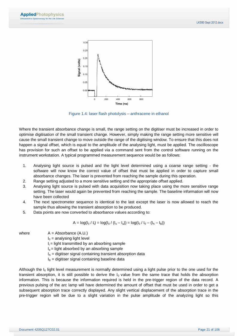
Figure 1.4: laser flash photolysis – anthracene in ethanol
Where the transient absorbance change is small, the range setting on the digitiser must be increased in order to
optimise digitisation of the small transient change. However, simply making the range setting more sensitive will
cause the small transient change to move outside the range of the digitising window. To ensure that this does not
happen a signal offset, which is equal to the amplitude of the analysing light, must be applied. The oscilloscope
has provision for such an offset to be applied via a command sent from the control software running on the
instrument workstation. A typical programmed measurement sequence would be as follows:
1. Analysing light source is pulsed and the light level determined using a coarse range setting - the
software will now know the correct value of offset that must be applied in order to capture small
absorbance changes. The laser is prevented from reaching the sample during this operation.
2. Range setting adjusted to a more sensitive setting and the appropriate offset applied.
3. Analysing light source is pulsed with data acquisition now taking place using the more sensitive range
setting. The laser would again be prevented from reaching the sample. The baseline information will now
have been collected
4. The next spectrometer sequence is identical to the last except the laser is now allowed to reach the
sample thus allowing the transient absorption to be produced.
5. Data points are now converted to absorbance values according to:
A = log(I0 / It) = log(I0 / (Io – Ia)) = log(I0 / I0 – (IA – IB))
where A = Absorbance (A.U.)
I0 = analysing light level
It = light transmitted by an absorbing sample
Ia = light absorbed by an absorbing sample
IA = digitiser signal containing transient absorption data
IB = digitiser signal containing baseline data
Although the I0 light level measurement is normally determined using a light pulse prior to the one used for the
transient absorption, it is still possible to derive the I0 value from the same trace that holds the absorption
information. This is because the information required is held in the pre-trigger region of the data record. A
previous pulsing of the arc lamp will have determined the amount of offset that must be used in order to get a
subsequent absorption trace correctly displayed. Any slight vertical displacement of the absorption trace in the
pre-trigger region will be due to a slight variation in the pulse amplitude of the analyzing light so this

Document 4205Q127C02.01 Page 22 of 106
LKS80 Sept 2012.docx
displacement can then be measured and used to make a slight adjustment to the I0 value that had previously
been used to generate the offset command i.e. the final I value was determined on the same data record that
contains the absorption data.
The above method provides a simple and reliable way of obtaining laser flash photolysis data even where the
transient absorbance is small i.e. absorbance change less than 0.01 AU or transmission change of less than 3%.
However, it does require the use of a digital oscilloscope where it is possible to completely offset the light level
for all the signal ranges that are likely to be used.
In some cases, it is also possible to use information contained in the pre-trigger region of the data trace to
determine the baseline reference. When this can be done (i.e. usually with timescales in the region of 200
ns/div), there is then no absolute need to acquire a baseline trace for subsequent subtraction. On longer
timescales, subtraction of baseline data means that any small perturbation of the pulsed light profile will be
removed, provided that it is consistent and present in the same place on both the baseline and the transient data
trace. The records in (Figure 1.5) demonstrate this. The record on the left shows the full width of the plateau
region with about 1.5% total signal variation. The trace on the right is after processing to absorbance (including
baseline subtraction).
Figure 1.5: pulsed xenon light source plateau region before (left) and after (right) baseline correction and
conversion to absorbance
An alternative method, using a track-and-hold circuit, had previously been used before the digital oscilloscopes
became available with programmable offset capabilities. In the track-and-hold device, the arc lamp pulse is
continually tracked with current injected into the signal line from the photomultiplier to force the resultant signal to
zero volts. A measure of the light level amplitude can be derived from knowledge of the injected current. Just
prior to the laser output, signal tracking would be halted and then all subsequent changes in light level would be
recorded including those due to the transient absorption. Although functional, this technique can lead to noise
problems as the electronic track-and-hold circuit needs connection directly into the photomultiplier signal circuit.
The offset method currently used in the LKS80 spectrometer has the advantage that the photomultiplier signal is
brought directly to the signal input of the digital oscilloscope.
1.3.4 Signal Offset (additional notes)
The rationale behind applying a signal offset in order to access small absorption changes is illustrated in Figure
1.6, which shows the situation where the analysing light level is -500 mV and the transient absorption accounts

Document 4205Q127C02.01 Page 23 of 106
LKS80 Sept 2012.docx
for a maximum of 10% of this signal level. Increasing the sensitivity setting of the signal digitiser by a factor of 5
(i.e. to 20 mV/div) would only access data that lies between 0 V and -0.1 V.
Figure 1.6: analyzing light signal of -500 mV without offset or rescaling
Figure 1.7 left shows the result of applying a signal offset which is equal and opposite to the magnitude of the
analysing light level. In addition, the vertical position of the 0 V level (i.e. signal ground) has been shifted from the
top of the screen display towards the bottom. With offset applied and the data trace repositioned, the input
sensitivity of the signal digitiser can then be increased so that the absorption signal fills the digitiser window
(Figure 1.7 right)
Figure 1.7: signal display with offset (left) and with offset and rescaling (right)

Document 4205Q127C02.01 Page 24 of 106
LKS80 Sept 2012.docx
2 HARDWARE
2.1 LKS80 layout
A typical layout plan for the spectrometer is shown in Figure 2.1. Although the figure shows the LKS.60
instrument, the LKS80 layout is very similar. The modular form of the instrument allows some flexibility with
respect to the layout so that different lasers can be accommodated. The latest compact head Nd:YAG lasers
allow much smaller layout formats to be adopted.
Figure 2.1: typical layout for the LKS80
In this example, the laser is a model Brilliant Nd:YAG from Quantel that has been fitted with 2nd and 4th
harmonic generators. The power supply for the laser is sufficiently compact to allow it to be sited under the
support table for the spectrometer. Where space allows, the "L" shaped arrangement is undoubtedly the most
convenient way to set up the instrument. A laser pulse duration of around 4 to 6 ns can be expected for this type
of instrument.

Document 4205Q127C02.01 Page 25 of 106
LKS80 Sept 2012.docx
2.2 Pulsed xenon light source
The pulsed xenon light source comprises a high stability, power controlled lamp supply used to drive a 150 watt
xenon short arc lamp mounted in a convection cooled housing. The output from the light source is increased by
at least 50 times in the visible and 150 times in the UV. The pulsed light has a duration of about 1.5 ms and the
middle of the pulse is flat for 400 µs to within 4% and 100 µs to within 1%. A timing circuit allows the plateau
region to be synchronised with the laser output. (An extra timing circuit and output is available to allow for any
additional synchronisation that may be required.)
Figure 2.2: the components of the pulsed xenon light source
2.2.1 The Arc lamp power supply
The functions and displays of the arc lamp power supply are as follows
Front panel
MOMENTARY PUSH BUTTON provides power to igniter module
Rear Panel
COMBINED INPUT POWER, POWER SWITCH AND FUSE HOLDER: F1 is the line input fuse
F1 Fuse (110V - 120V) 5 A (T); 20 mm
F1 Fuse (200V - 240V) 2.5 A (T); 20 mm
VOLTAGE SELECTOR selection for 240, 220, 200, 120, 115, 100 mains voltage input
FUSEHOLDER (F2): output fuse (10 A; 1¼")
IGNITE: 4 pin socket which provides power to igniter module
D.C. OUTPUT: provides the stabilised output to the lamp
CR/W4: slide switch, two positions according to lamp type
EARTH TERMINAL: used to connect earthing braid from lamp housing.

Document 4205Q127C02.01 Page 26 of 106
LKS80 Sept 2012.docx
2.2.2 Lamp Housing
The lamp housing features an off-axis optical design (Figure 2.3). The result is a very high throughput with a
clearly defined arc image. Immediately in front of the xenon lamp is a cylindrical lens which helps to sharpen the
image by minimising the astigmatism caused by the off-axis spherical mirror.
The functions and displays of the lamp housing are as follows
SHUTTER: a slide shutter mounted in the output port
GAS PURGE PORT on the right of the lamp housing is a angled connector which can be attached to a
nitrogen supply should a xenon lamp with a Spectrosil envelope be fitted (i.e. the lamp is ozone
producing).
VERTICAL LAMP ADJUSTER at the top of the lamp housing is an access port (fitted with a slotted
PEEK plug). Removal of this plug allows the lamp vertical position to be adjusted (Section 2.11.5) using
the special insulated hexagonal wrench.
HORIZONTAL LAMP ADJUSTER: on the left face of the lamp housing (i.e. the face with the output port)
is the plugged access port for horizontal lamp adjustment.
Figure 2.3: the optical layout of the xenon light source
2.2.3 Lamp Type
The lamp that is normally fitted to the LKS80 instrument is the ozone free xenon arc lamp manufactured by
OSRAM (type 150W/CR OFR). The Hamamatsu type L2273 is an alternative lamp which has similar electrical
characteristics. It has a Spectrosil bulb and is recommended for use where increased performance in the 200 to
300 nm region is required.
2.2.4 Lamp Pulser
The arc lamp pulser contains a 10 stage, LC pulse forming network (PFN) which is charged to a preset voltage
prior to discharge through the lamp. The shape of the arc lamp pulse can be modified by the relative position of
a tuning component in relation to the PFN coils (accessed via the rear panel). Capacitor charge voltage has an
effect on pulse flatness and pulse intensity.

Document 4205Q127C02.01 Page 27 of 106
LKS80 Sept 2012.docx
Front panel
Figure 2.4: the arc lamp pulser front panel
The arc lamp pulser front panel is shown in Figure 2.4. The functions and displays are as follows:
POWER: latching, push button power on switch
ENERGY: single turn voltage control to determine charge voltage on PFN capacitors
PULSE ENERGY: analogue display (0 to 150 volts)
PULSE LAMP: momentary push button - provides power to igniter module
DISABLE: latching switch which allows capacitor charge circuit to be disable whilst allowing the SYNC
PULSE DELAY circuit to remain active
SYNC PULSE DELAY: 10 turn control to set position of the SYNC output pulse (+1 to +11ms relative to
trigger point)
LAMP PULSE DELAY: 10 turn control to move timing of the arc lamp pulse relative to the position of the
laser output (+1 to +11ms relative to trigger point)
Rear panel
Figure 2.5: the arc lamp pulser rear panel

Document 4205Q127C02.01 Page 28 of 106
LKS80 Sept 2012.docx
The arc lamp pulser rear panel is shown in Figure 2.5. The functions and displays are as follows:
POWER INPUT - standard IEC type line input socket
LINE FUSE -
120/240 - two position voltage selector (120 volts or 240 volts)
EXT TRIGGER - BNC socket for trigger input (+5 volt, TTL)
SYNC OUTPUT - BNC socket providing 5 volt SYNC output pulse which can be set to occur at a
minimum of 1ms and maximum of 10ms following the receipt of an EXTERNAL TRIGGER signal or
operation of the push button trigger.
DC INPUT - 3-pin socket which receives the DC output from the lamp power supply
DC OUTPUT - 3-pin socket for connecting the lamp housing to the lamp supply
ADJUST - push/pull facility for setting tuning element position with respect to PFN.
2.2.5 Pulsed light source performance
150 times increase in signal in the UV region
35 times increase in signal in the visible region
2 ms overall pulse duration
400µs plateau region following tuning of the pulse-forming-network
Plateau flat to within +/- 0.5% flatness for at least 100µs (typically 250 µs).
Plateau flat to within +/- 0.1% for at least 1µs
Pulse-to-pulse amplitude reproducibility is as follows:
90% of shots within +/- 0.2%
96% of shots within +/- 0.5%
100% of shots within +/- 0.8%
2.3 Electronics unit
The electronics unit contains a number of plug-in modules for controlling the various operations of the laser flash
photolysis instrument.. It is fitted with a single IEC type line input socket.
2.3.1 Front panel
Figure 2.6: the electronics unit (front)

Document 4205Q127C02.01 Page 29 of 106
LKS80 Sept 2012.docx
The electronic unit front panel is shown in Figure 2.6. The functions and displays are as follows
SYSTEM – rocker style power switch.
STATUS – green indicator lamp which will be continuously illuminated if the unit has passed all its self-
checks. A flashing green light will indicate either a failure of a self-test or a missing motor drive plug-in
card.
TX – red indicator lamp which becomes illuminated when the unit is transmitting to the computer work
station.
RX - red indicator lamp which becomes illuminated when the unit is receiving data from with the
computer work station.
2.3.2 Rear panel
Figure 2.7: the electronics unit (rear)
The electronics rear panel is shown in Figure 2.7. The functions and displays are as follows:
POWER INPUT PANEL: IEC type line input socket with separate 20 mm, 1 amp fuse holder (mains input
range 85 to 264 VAC, 47 to 63 Hz).
12 V and 5 V SUPPLY MODULES: these modules do not connect to the laser spectrometer, the 2 mm
panel sockets are for test purposes only..
USB COMMUNICATIONS MODULE: This module is connected to a USB socket on the computer
workstation via the socket marked TX / RX. The sockets labeled DRIVE and TEMP INPUTS are not
used on the LKS80 laser spectrometer.
CONTROL MODULE 1: This module provides control of the monochromators. For system configuration
with a single monochromator, the monochromator must be connected to the Drive 1 port. For
configurations have two monochromators, the second monochromator should be connected to the Drive
2 port.
LF MODULE: This module provides the timing control of the various activities that comprise the laser
flash photolysis spectrometer operating sequence.
HV O/P: type H4, high voltage BNC socket providing the high voltage output (up to 1200 volts) for the
photomultiplier detector.
LASER SYNC: BNC socket which provides a 5 volt output pulse which can be used for synchronising an
extra external event. The position of the pulse in the timing sequence can be set from a software
configuration panel on the workstation. Whenever the laser flashlamp is run repetitively (i.e. at 10 or 20
Hz from LASER TRIG socket), the LASER SYNC output is used to provide a Q-switch trigger pulse. The

Document 4205Q127C02.01 Page 30 of 106
LKS80 Sept 2012.docx
correct timing values must then be entered into the software configuration panel. The pulse is usually
set to be + 5 volts but the pulse characteristics can be changed from within the software configuration
panel. (A negative edge trigger pulse can be configured when required i.e. 5 V to 0 V).
LASER TRIG: BNC socket which provides the flashlamp trigger pulse to the laser power supply. The
pulse is usually set to be + 5 volts but the pulse characteristics can be changed from within the software
configuration panel. (A negative edge trigger pulse can be configured when required i.e. 5 V to 0 V).
PULSER: BNC socket which provides the 5 volt trigger pulse for the arc lamp pulser.
LASER ENERGY: BNC socket which is connected to the output from the integrating photodiode
(photodiode optical module).
PD POWER: provides the low voltage to operate the integrating and trigger photodiodes.
LAMP SHUTTER: socket for connecting the shutter drive to the shutter located inside the sample
housing which controls the entry of the analyzing light into the sample housing.
LASER SHUTTER: socket for connecting the shutter drive to the shutter located at the rear of the
sample housing at the entry port for the laser actinic light.
MAN CTRL: socket for connecting to the remote switch control panel.
AUX: expansion socket.
2.3.3 Remote switch panel
The functions of the remote switch panel are as follows:
LASER SHUTTER: push button selection of three functions which provide overall control of the laser
shutter at the rear of the sample housing. Functions are as below.
o CLOSED: shutter is kept closed during a spectrometer cycle.
o NORMAL: shutter will open in a sequence initiated by the START: switch or control command
from the computer workstation.
o OPEN: shutter will be forced into the open position. Neither the START switch nor an incoming
control pulse has any effect on its open state.
LAMP SHUTTER: push button selection of three functions which provide overall control of the shutter in
the sample housing that blocks the passage of the analysing light. Functions are as above.
EXT / INT: push button selection of EXT and INT functions. The EXT selection allows closure of the
lamp shutter to be determined by the LKS software according to the data acquisition time period. With
the INT selection, shutter closure is determined by the timing selected within the LF MODULE.
0.1s / 1s / 10s: push button selection of three shutter closure times which come into operation when the
EXT / INT selector is set to the INT position.
LASER TRIGGER: push button selection of DISABLE and ENABLE functions with respect to the
flashlamp trigger output to the laser power supply. The ability to disable the trigger output is particularly
useful when the spectrometer controller is configured to repetitively trigger the laser flashlamp at 10 or
20 Hz.
LAMP TRIGGER: push button selection of the DISABLE and ENABLE functions with respect to pulsing
of the analysing light (xenon arc lamp).
START: push button switch used to initiate a spectrometer sequence.
2.3.4 Configuration and timing
The Electronics Unit can be configured via the computer workstation for operation with single shot, 10 Hz or 20
Hz optimized lasers. When working with a single shot optimized laser, the Electronics Unit provides a single
trigger pulse to externally trigger the laser flashlamp and, in this case, the laser Q-switch is configured for internal
trigger operation.
For a laser that is optimized for 10 Hz or 20 Hz flashlamp operation, only the occasional Q-switched laser output
would be needed for normal flash photolysis operation. The Electronics Unit provides a 10 Hz or 20 Hz pulse

Document 4205Q127C02.01 Page 31 of 106
LKS80 Sept 2012.docx
train to keep the laser flashlamp running according to the laser’s optimised parameters. Q-switched operation
takes place when a Pockels cell is switched at a precise moment after the laser pump flash has occurred.
Provided that this optimized time delay is known and provided that the laser can have its Q-switch operation
initiated from an external trigger pulse, the spectrometer controller timing can be set so that a SYNC pulse is
provided at exactly the time that the Q-switch trigger pulse is required by the laser. In this way, a Q-switched
laser pulse will only occur when a spectrometer measurement sequence is initiated.
Although the primary timing with respect to pulsing the arc lamp is set by the Electronics Unit, the final
positioning of the arc lamp pulse relative to the laser output is set using the LAMP PULSE DELAY control on the
front panel of the arc lamp pulser.
Figure 2.8: timing diagram illustrating the sequence of operations

Document 4205Q127C02.01 Page 32 of 106
LKS80 Sept 2012.docx
The timing diagram (Figure 2.8) is divided into three sections according to instrument function. Two sets of
shutter control lines are shown. The second pair show the levels that would be seen when the shutter operation
is to be disabled i.e. shutter(s) remaining closed.
The second section shows an overview of activity within the spectrometer controller and the third section shows
the activity within the arc lamp pulser. The bottom section shows the oscilloscope trigger signal that is produced
from the photodiode trigger assembly when it sees laser light on its way to the sample housing.
2.4 Interlock unit
Figure 2.9: the interlock unit
The function of the interlock unit (Figure 2.9) is to protect against the accidental application of a xenon lamp
ignition pulse whilst other electronic equipment is switched on. Whilst the spark gap arc lamp igniter is not
normally expected to be a hazard to electronic modules located in the immediate vicinity of the lamp housing, it is
sensible to have a precautionary measure in place to ensure protection against possible damage. The time that
such damage might occur to other powered up electronic modules would be when the lamp becomes more
difficult to start due to lamp ageing or the electrode gap in the igniter becoming too large.
The interlock unit is connected to the arc lamp ignition circuit so that lamp ignition can only be attempted when
the interlock unit is not switched on. When the unit is switched on, a contactor module disables the ignition circuit
and connects mains voltage, via the output cable, to the main instrument power distribution board. The functions
and displays are as follows:
CONNECTIONS
- ignition circuit input
- ignition circuit output
- mains power in (IEC socket)
- mains power out (flying lead to power distribution board)
PANEL CONTROL: illuminated mains power switch
FUSEHOLDER: 10 A, 1¼"

Document 4205Q127C02.01 Page 33 of 106
LKS80 Sept 2012.docx
2.5 Sample housing
2.5.1 Introduction
The sample housing has overall dimensions of 400 x 300 x 170 mm. This size provides sufficient size for
accommodating accessories such as the diffuse reflectance accessory and the flow-flash configuration.
Programmable electronic shutters are mounted in the beam paths of the laser and the analysing light. Sample
optics are mounted on a mini optical rail with adjustable x, y, z mounts. Variable aperture stops are fitted on
either side of the sample holders so that the dimensions of the analysing beam can be matched to the laser
beam profile. The sample holder can be offset in its mount so that the probe beam can be set to pass close to
the face of the cuvette that is in the laser beam path (i.e. where the highest concentration of the transient species
will occur). The sample optics can be configured for either cross beam or co-linear excitation (a prism assembly
is provided for combining the laser and analysing light beams when co-linear accessory is used). A laser beam
dump, with a magnetic base, can be placed in a suitable position on the front wall of the sample housing in order
to catch the laser beam after it has passed through the cuvette. The sample housing is fitted with filter holders
where the analysing light enters and leaves the sample housing. A 10 x 10 mm cuvette with thermostatable
sample holder is provided for use in the cross beam configuration and a cylindrical cell (20 mm optical path) with
sample holder is provided with the co-linear accessory.
2.5.2 Cross beam configuration
Figure 2.10: sample housing in cross beam configuration
The sample housing is shown set up in the cross beam configuration in Figure 2.10. A mini optical rail is
mounted on the baseplate and this is used to mount components along the spectrometer‘s optical axis. The
thermostated sample holder, which accommodates a standard size, 10mm path length, spectrometer cuvette, is
located at the midpoint of the rail. On either side of the cell position there are two lens holders. Each of these
lens holders has x, y, z adjustment. Between the laser shutter and the sample position is an adjustable rail which
has a single lens holder mounted on it. In most cases this is supplied without a lens fitted and is intended as a
spare mount that can be used should a lens be required for some special arrangement. Either side of this
adjustable rail there are storage locations for components not used in the cross beam configuration (i.e. to the

Document 4205Q127C02.01 Page 34 of 106
LKS80 Sept 2012.docx
left is the holder for the 20 mm path length cylindrical cell and to the right is the beam splitter mount that is used
to combine the laser and the analysing light).
2.5.3 Co-linear configuration
Figure 2.11: sample holder in colinear configuration
The alternative way of configuring the sample housing is illustrated in Figure 2.11. In the co-linear configuration,
a prism mount is positioned on the mini-rail to the left of the mid line. The adjustable rail is set to subtend an
angle of 78° to the spectrometer axis. This angled rail assembly is then used as a guide for the incoming laser
beam. The use of a beam splitter in this way means that there is some loss of laser intensity reaching the sample
and also some loss of the analysing light as well. The 78° angle optimises the beam splitter performance in terms
of minimising the losses. The beam splitter mount is attached to a gearbox so that the prism angle can be readily
adjusted. The advantage of the colinear arrangement is the ability to make use of a longer sample pathlength. A
cylindrical cell holder is shown in place of the 10 mm sample holder.
2.5.4 Filter holders
The filter holders can be seen on either side of the sample housing. They can be used as follows:
Either a colour glass cut-off filter or an interference filter can placed in the right hand filter holder in order
to protect the sample from the intense broad band output from lamp housing during the period that the
electronically controlled optical shutter is open.
A suitable colour glass cut-off filter placed in either filter holder in order to prevent monochromator
second order effects being seen by the photomultiplier (i.e. if monitoring 700 nm, a 400 nm cutoff filter
would be needed to prevent some 350 nm radiation from passing through to the detector).
A suitable blocking filter placed in the right hand filter holder to prevent laser light from passing into the
lamp housing when using the colinear sample configuration.

Document 4205Q127C02.01 Page 35 of 106
LKS80 Sept 2012.docx
2.6 Monochromator
The high precision automated monochromator is shown in Figure 2.12.
Figure 2.12: the monochromator
The monochromator contains a 250 nm holographic diffraction grating that provides a useful operating
wavelength range of 190 to beyond 850 nm (limited by PMT detector range). The monochromator is accurately
pre-aligned and calibrated using a He-Ne laser and mercury emission lines.
The wavelength of monochromatic light is selected by rotation of the grating using a stepper motor housed within
the monochromator unit. This motor is controlled via Control Module 1 in the Electronics Unit. This allows the
monochromator wavelength to be set via the LKS control software.
The wavelength of monochromatic light is selected by rotation of the grating using a stepper motor housed within
the monochromator unit. This motor is controlled via Control Module 1 in the Electronics Unit. This allows the
monochromator wavelength to be set via the LKS control software.
To allow for light level optimisation, the monochromator is fitted with continuously variable bi-lateral slit
assemblies. The monochromator entrance and exit slits are manually adjustable using the dials on the front of
the monochromator. A 1 mm monochromator slit opening is equivalent to a wavelength bandwidth of 4.65 nm.
The slits provide a bandwidth range from below 0.5 nm up to 37 nm. By opening the slits, the light throughput
can be increased at the expense of bandwidth. A slit width of around 0.5 mm is suitable for most measurements.
Light-tight flanges are fitted to the monochromator entrance and exit ports,.
The monochromator control cable is connected to Port 1 of Control Module 1 in the Electronics Unit. For systems
with two monochromators, Mono 1 must be connected to the Drive 1 port and Mono 2 must be connected to the
Drive 2 port.
Locking Screws
Entrance
Slit Control
Exit Port
Exit Slit
Control

Document 4205Q127C02.01 Page 36 of 106
LKS80 Sept 2012.docx
Monochromator Specification
Aperture ratio: f/3.4
Optical configuration: Symmetrical Czerny-Turner
Grating type: Holographic
Grooves/mm: 1200
Dispersion: 4.65 nm/mm
Slits: Continuously variable, bilateral
Slit opening: 0.1mm to 8mm (about 35nm)
Wavelength drive: Stepper motor
Step resolution: 0.1nm
Scanning range: 200 to 1000nm
Wavelength control: Remote
2.7 Signal detection
For signal detection, a photomultiplier housing is attached to the exit light port of the monochromator. Inside this
detector housing is mounted either a R928 or 1P28 side window photomultiplier, µ-metal shield, focusing optic
and low gain, high linearity, five stage circuit designed for high current pulsed mode operation (absorption
measurements). The detector module is driven from a 10 mA, 10 to 1200 volt programmable photomultiplier
power supply (located in the spectrometer controller). The 1P28 has a range 200 – 630 nm and the R928 range
extends the range further to the red (to about 850 nm). Although the same photomultiplier housing can be used
for laser induced emission measurements it is recommended that a similar housing be used which is optimised
for emission measurements. The base circuit in this module does not use the Zener diodes which are important
part of the photomultiplier housing that is optimised for transient absorption measurements when using a pulsed
xenon light source.
The 5-stage photomultiplier housing is illustrated in Figure 2.13 with the left picture showing the signal socket
and the high voltage BNC socket. The middle picture shows the male flange with captive fasteners by which the
housing is attached to the monochromator. The picture on the right shows the inside of the unit with the µmetal
shield in place around the photomultiplier. Changing the photomultiplier tube simply requires that the shield
clamp be loosened to first remove the shield then the R928 (plug-in compatible) can be mounted in place of the
1P28.
Figure 2.13: the 5-stage photomultiplier housing front (left), rear (centre) and interior (right)
The spectral plots in Figure 2.14 represent the instrument response curves produced using the xenon light
source (unpulsed) as modified by the transmission characteristics of the monochromator and the response curve

Document 4205Q127C02.01 Page 37 of 106
LKS80 Sept 2012.docx
of the photomultiplier (both 1P28 and R928). Both plots show unfiltered analysing light and also light having
passed through a GG420 colour glass cut-off filter. In the near infrared region, a reduction in relative signal level
can be seen and is caused by the removal by the filter of those wavelengths that would otherwise have been
able to transmit at double the wavelength (i.e. the diffraction grating second order effect according to the Bragg
equation n= 2d.sin). The effect of the second order filter can be seen more clearly in graphs below which are
zoomed into the near IR region. Beyond 840nm, the signal from the filtered light is seen rising again. In the case
of the 1P28, the extra signal due to second order stray light at wavelengths longer than 640nm shows clearly
whereas this second order light is reduced to zero with the second order filter in place. In the case of the R928,
there is still a significant amount of signal at 750nm even when the GG420 filter is in place as one would expect
because of the R928’s extended red response.
Figure 2.14: spectral characteristics of the xenon lamp with PMT 1P28 (left) and R928 (right)
Figure 2.15: 2nd
order stray light, PMT 1P28 (left) and R928 (right)

Document 4205Q127C02.01 Page 38 of 106
LKS80 Sept 2012.docx
Provided second order precautions have been taken, it should be possible to make laser flash photolysis
measurements up to about 850 nm as is demonstrated by how well the xenon spectral lines are picked up in the
650 and 850 nm region.
2.8 Photodiode trigger/energy monitor
This module (Figure 2.16) is located in the beam path of the laser output. As the laser light passes through the
module, a very small amount of the laser beam is reflected by a quartz beam splitter in the direction of a white
ceramic plate. The ceramic plate acts as a light diffuser and some of this diffused light falls upon two
photodiodes (trigger photodiode and integrating photodiode). The trigger photodiode provides a fast trigger pulse
which is used to provide the zero time trigger to the digital oscilloscope. The circuit associated with the
integrating photodiode allows the signal produced from the laser pulse to be drawn out to a duration which can
be readily digitized by a 100 kHz ADC converter located in the instrument workstation. The instrument software
then calculates the area under the curve of this extended pulse profile and this is used to provide an indication of
the shot-to-shot relative laser intensity.
Figure 2.16: the photodiode trigger/energy monitor exterior (left) and interior (right)
2.9 Laser beam steering module
The laser beam steering module is shown in Figure 2.17. The laser head is normally positioned parallel to the
optical axis of the laser flash photolysis spectrometer. The beam steering optic is used to direct the laser output
towards the sample position so that it subtends an angle at the optical axis of 90° for the cross beam
configuration or 78° for the colinear configuration. A Pellin-Broca type right angled prism is used to steer the
laser and this ensures that there is no risk of a potentially harmful reflection being directed back towards the
laser cavity. The prism is attached to an adjustable mount which can be accessed when the cover is removed
(held in place by four finger screws). This adjustment ensures that the laser can be targeted precisely onto the
point where the analysing light passes through the sample.

Document 4205Q127C02.01 Page 39 of 106
LKS80 Sept 2012.docx
Figure 2.17: the laser beam steering module exterior (left) and interior (right)
2.10 Digitising oscilloscope
The signal output from the spectrometer‘s photomultiplier is digitised by a programmable digital oscilloscope. The
recommended model is the Agilent DSO9064A Infiniium oscilloscope which has the following overall
specification:-
Digitising rate up to 5 GSa/s (i.e. 0.2 ns between data points)
Bandwidth 600 MHz
Resolution 8 bit
DC offset programmable
Pre-trigger yes
Interface USB
Address 7
All functionality required to acquire absorption data down to absorbance values of <0.01 AU is under direct
control of the spectrometer workstation.
The default address of the Infiniium series oscilloscope is 7. If for any reason this is changed, the
workstation software will not be able to communicate with the oscilloscope.

Document 4205Q127C02.01 Page 40 of 106
LKS80 Sept 2012.docx
2.11 Instrument installation
2.11.1 Layout
The LKS80 laser flash photolysis spectrometer is a modular instrument and so there is some flexibility in the way
that the instrument is set up. Although the preferred layout is the L-shaped plan shown in Figure 2.18, available
space, type of laser etc. can necessitate changes to this layout plan.
Figure 2.18: a typical layout plan for the LKS80 laser flash photolysis spectrometer
2.11.2 Installation requirements
The installation requirements for the LKS80 are described in the Installation and Operational Requirements
section of this User Manual (page 7). A typical layout is shown in Figure 2.1.
2.11.3 Instrument layout
The design of the laser flash photolysis sample housing requires that the Nd:YAG laser be positioned parallel
and to the rear of the main optical rail. In principal, the laser head could point either right to left or right depending
on space availability or which arrangement gives most convenient access to adjustments on the harmonic
generators (when using a Nd:YAG laser). Normally the laser is set pointing in the same direction as the xenon
light source.
If the laser is a compact Nd:YAG laser, then this will normally be attached to a saddle that is mounted on an
optical rail set behind the spectrometer rail. The two rails are securely linked together. In front of the laser will be
a saddle assembly that mounts the photodiode module and the laser beam steering assembly. In cases where
the laser is too large to be mounted in this way, there will be a shorter length of rail to accommodate just the
saddle with the photodiode and laser beam steering modules.

Document 4205Q127C02.01 Page 41 of 106
LKS80 Sept 2012.docx
The xenon lamp should be placed to the right of the sample housing ensuring that the lamp housing distance
piece is located between the lamp housing mechanical shutter and the sample housing (its function is to prevent
the arc lamp output from being focused onto the blades of the electro-mechanical shutter).
The lamp power supply and arc lamp pulser should be located to the right of the lamp housing with the lamp
housing earth connected to the rear of the lamp power supply. The DC output from the lamp power supply is
connected directly to the arc lamp pulser and the pulser is connected directly to the lamp housing.
The digital oscilloscope should be positioned immediately to the left of the optical rail so as to keep the signal
connection from the photomultiplier as short as possible.
An interlock unit is supplied and it is from this unit that the power is derived for all the electronic modules that
make up the instrument. Only when the interlock unit is switched off (i.e. no power distributed to the instrument)
is it possible to ignite the xenon arc lamp. Once the interlock unit is switched on, the start pulse for the arc lamp
is disabled. The ‘Igniter’ output from the lamp power supply (i.e. the socket which brings power to the igniter)
should be connected via the interlock unit. The power for all other equipment is supplied via a power distribution
board which is attached to the rear of the interlock unit via the output flying lead.
2.11.4 Instrument connections
The schematic (Figure 2.19) and table (Table 2.1) summarise how the various modules in the laser flash
photolysis spectrometer are linked together. This arrangement applies to the situation where the laser is a
Nd:YAG (optimised for single shot operation) or an excimer laser. In the case of a 10Hz or 20Hz Nd:YAG laser,
there would be an extra connection between the spectrometer controller and the laser to provide the capability of
Q-switching the laser on demand.
Figure 2.19: schematic of the laser flash photolysis spectrometer

Document 4205Q127C02.01 Page 42 of 106
LKS80 Sept 2012.docx
Table 2.1: LKS80 module connections
2.11.5 Fitting or changing the arc lamp
The arc lamp replacement bulbs are supplied by outside companies. Read the safety and other information
provided with the bulbs by the suppliers, and observe the precautions described there and below.
The xenon arc lamp that produces intense ultraviolet radiation that can irritate the eyes and may
impair eyesight. Never look directly at the light source. Do not open the lamp housing while the
lamp is operating or immediately after it is powered off. Do not allow the skin to be exposed to
UV radiation.
The xenon arc lamp runs at high temperatures and at an operating pressure of several
atmospheres. Xenon arc lamps can explode if mishandled. Wait for the lamp to cool down before
handling. Wear safety goggles or a safety visor when handling the lamp.
The ignition voltage for the arc lamp is 20 kV to 30 kV. To avoid the possibility of shock, stay at
least half a metre away from the lamp power cables during ignition.

Document 4205Q127C02.01 Page 43 of 106
LKS80 Sept 2012.docx
If the lamp bulb comes into contact with the skin, hotspots can be formed which cause the lamp
to fail. If the bulb does come into contact with the skin, or if any other dust or grime adheres to
the bulb, see the suppliers instructions for cleaning.
The arc lamp housing is shown in Figure 2.20.
Figure 2.20: lamp housing exterior (left) and interior (right)
To fit or replace a bulb, follow these steps:
1. Disconnect all the cables and remove the lamp housing from the optical rail. As the lamp operates at a
very high internal gas pressure it is very important that it is only handled when cold and protective
equipment (especially a face visor) is worn.
2. Remove the rear panel by undoing the four corner screw fasteners. Loosen the clamp screw on the
anode mounting block so that the top of the lamp can move freely, then remove the cable and the
cathode heat sink from the bottom of the lamp. (Before removing the heat sink make a note of its
orientation.)
3. It should now be possible to remove the lamp from the top clamp. Loosen the alignment fixing screw on
the back of the plate and adjust the horizontal and vertical adjusters so that they are approximately in the
centre of their travel.
4. Fit the new lamp into the anode mounting block but do not tighten the clamp screw yet.
5. Fit the cathode heat sink (in the correct orientation with the vanes pointing upwards towards the lamp
bulb) and attach the cable to the bottom of the lamp. Note that a washer is used to ensure that the
attached cable and heat sink are well secured.
6. Adjust the vertical position of the lamp so that the gap between the electrodes is level with the two
alignment pillars. Now tighten up the clamping screw on the anode mounting block. Check again that the
gap between the electrodes is vertically level with the two alignment pillars and horizontally level with the
centre spot. If this is not the case adjust the horizontal and vertical position of the lamp using the
adjusters shown in the diagram.
7. Make sure that you remember to tighten up the fixing screw on the back of the lamp backplate when you
have finished so as to secure the lamp adjustment assembly.
8. The rear panel can now be refitted to the back of the lamp housing using the four corner screws.

Document 4205Q127C02.01 Page 44 of 106
LKS80 Sept 2012.docx
Lamp Adjustment
Fine tune the alignment of the lamp by first loosening the alignment fixing screw set into the heat sink at the rear,
remove the adjuster screw plastic cover plugs and carefully adjust the vertical and horizontal alignments whilst
monitoring the signal output from the photomultiplier. It is very important that the adjustment is made using the
red insulated hexagonal driver, so that there is no risk of electrical shock. This will also ensure that the anode
block cannot be shorted to earth. Once the alignment is complete, the locking screw should be tightened and the
adjuster screw plastic cover plugs replaced.
Lamp Shutter
The shutter is closed when it is pulled to the front.
Lamp Stability
The lamp will take up to 30 minutes to stabilise after ignition and the lamp.
Lamp Replacement
The lamp should be replaced every 1000 operational hours or when its output becomes unstable.
2.11.6 Optical alignment
The LKS80 xenon arc lamp produces intense ultraviolet radiation that can irritate the eyes and
may impair eyesight. Never look directly at the light source. If it is necessary to remove the top of
the spectrometer to align the beam, wear UV protective eyewear while the lamp is on.
Optical re-alignment of the sample housing should not be necessary. However, if this needs to be checked
because one or more components have been disturbed, the following guidelines should help. If one is confident
that the lamp position is correct then step one can be missed out. If starting from step two then first check that
the monochromator entrance slit is set to 0.5 mm. (For a two monochromator instrument, monochromator one
slits could be set to 4 mm and monochromator two slits to 2 mm).
1. Check that the xenon lamp is correctly aligned within the lamp housing. The most effective way of doing
this is to arrange for the lamp housing to be directly coupled into the monochromator. For a single
monochromator instrument, this would need the sample housing to be removed from the spectrometer
rail and the monochromator moved so that it was directly in front of the lamp housing. The distance
piece should also be removed so that the lamp housing is directly coupled into the monochromator. For a
two monochromator instrument, there is a monochromator already coupled to the lamp housing
2. Ignite the arc lamp. Remove the four screws that hold the lid of the monochromator in place and then
remove the lid. Make sure that the monochromator slits are set to 0.5 mm. Check the illumination on the
first concave mirror in the monochromator (at the rear on the right) using a white business card carefully
positioned just in front of the mirror. If the illumination is uneven, unscrew the access plugs in the lamp
housing and use the insulated hexagonal wrench to adjust the position of the lamp as described in
Section 2.11.6.
3. Restore the lamp housing to its usual position (i.e. lamp housing, sample housing, monochromator on a
single monochromator instrument).
4. After first noting the relative positions of the various optical mounts, remove all the mounts from the mini-
rail within the sample housing (each mount is attached by a pair M4 captive fasteners).
5. The electronically controlled shutter (LAMP) should be opened using OPEN switch position on the
Spectrometer Controller.
6. The light observed within the sample housing should appear centred on the exit port (i.e. the left inside
wall).

Document 4205Q127C02.01 Page 45 of 106
LKS80 Sept 2012.docx
7. Replace the lens mount that is normally located on the far left of the mini rail (i.e. lens 4). Its mount
should be aligned with the end of the rail. Observe the light falling on the first concave mirror of the
monochromator using a white business card. The appearance of the light should be a narrow band that
is symmetrical and centred on the mirror. If the light is curved then the two M3 socket headed screws
should be loosened to allow the lens to be moved slightly towards the front or towards the rear, When
the best position has been found, tighten the two M3 screws. Also check that the height of the lens
holder looks optimal. Reset the height of the lens holder if necessary.
8. Now place the mount with the smallest diameter lens (i.e. lens 1) to the far right of the mini optical rail i.e.
about 10 mm in front of the shutter housing. Again observe the light falling on the first concave mirror.
Adjust the lens mount both forwards / backwards and vertically so as to optimize the light falling on the
mirror.
9. Place lens 3 on the mini rail, approximately 75 to 80 mm to the left the sample position (i.e. where the
laser will intersect the analysing light). Again, adjust the lens mount so as to optimise the appearance of
the light falling on the concave mirror.
10. Place lens 2 on the mini rail, approximately 75 to 80 mm to the right of the sample position. Again, adjust
the lens mount so as to optimise the appearance of the light falling on the concave mirror.
11. Now return the 10 mm sample holder back to its position in line with the laser port and laser axis. Initially
fully open the adjustable apertures. Gradually close these apertures down to about 3 to 4 mm (about the
optimum size when using crossed beam laser excitation) and observe how illumination on the
monochromator concave mirror has been affected. The area of illumination will be reduced but it should
be central and uniform. The position of the sample holder may need to be adjusted slightly to optimise
illumination of the monochromator optics (i.e. forwards / backwards or in a vertical sense).
12. Note that for crossed beam laser excitation, the 10 mm sample holder can be offset so that the analysing
light beam passes through the cuvette close to the face of the cuvette where laser is entering (this offset
is adjustable using the screw fixing at the bottom of the cuvette holder). For a reduced volume cuvette
(i.e. 10 x 4 mm internal dimensions) the thermostated cell block must be set in a central position so that
the analyzing light passes cleanly through the middle of the cuvette.
13. Set the laser so that it is Q-switching at 10 Hz with an increased flashlamp to Q-switch delay in order that
the laser energy is reduced to a level where it can just be seen on a piece of white business card.
14. Check that the laser output is correctly aligned with the photodiode / trigger module and also the Pellin-
Broca prism within the laser beam steering assembly.

Document 4205Q127C02.01 Page 46 of 106
LKS80 Sept 2012.docx
2.11.7 Laser alignment (crossed beam excitation)
The LKS80 xenon arc lamp produces intense ultraviolet radiation that can irritate the eyes and
may impair eyesight. Never look directly at the light source. If it is necessary to remove the top of
the spectrometer to align the beam, wear UV protective eyewear while the lamp is on.
Crossed beam irradiation of the sample is the simplest way of exciting the contents of the sample cuvette (refer
to Section 2.5.2). Adjustment of the laser beam requires the correct horizontal positioning of the saddle on which
the photodiode and beam steering modules are mounted. The final fine adjustment of the laser direction is made
using the two adjustments on the Pellin-Broca prism mount.
1. Set the laser running repetitively using the laser‘s repetitive operating mode and the output energy
reduced by way of an increased the flashlamp to Q-switch delay.
2. Cut a rectangular piece of white business card (about 85 x 11 mm) so that it will fit into the thermostated
cuvette holder. The cut card can then be used to make sure that the laser is aimed correctly at the
sample holder. When set at an angle, the card can also be used to check that the laser beam is at the
same height as the analyzing light passing through the sample holder.
3. At this stage, the cover of the beam steering prism module should be removed to allow the prism to be
adjusted. If a laser beam expander is also supplied (located between the laser shutter and the sample
position).
4. Using the shutter switches on the spectrometer control unit, ensure that both the laser and lamp shutters
are open (LAMP SHUTTER and LASER SHUTTER switches moved to the OPEN position).
5. On the Pellin-Broca prism mount, adjustment of the upper adjuster screw will cause the laser beam to be
moved in a horizontal direction. The lower adjuster screw will case the laser beam to be adjusted in a
vertical sense.
6. Using the prism mount screw adjusters and the piece of cut business card, adjust so that the laser beam
enters the sample block centrally and is at the same height as the xenon analyzing light beam.
7. A laser beam dump with a magnetic mount is provided. This should be attached to the inside surface of
the sample housing so that it catches the laser light that passes through the cuvette holder.
8. Set the variable apertures as required. (Opening to about 3 to 4 mm should be adequate. If the
aperture is too wide, any transient absorption will have its overall absorbance reduced as a result of light
that does not pass through that part of the solution excited by the laser. Too small an aperture setting
will impair signal-to-noise ratio due to attenuation of the analysing light intensity.)
9. A laser beam expander optic is sometimes used to increase the size of the laser beam width at the
sample position. If this optic has been supplied, it should now be mounted on the short length of optical
rail between the laser shutter and the sample position. Its position (height and lateral position) should be
adjusted so that the laser beam is still correctly aligned with the analysing light at the sample position.

Document 4205Q127C02.01 Page 47 of 106
LKS80 Sept 2012.docx
2.11.8 Laser alignment (co-linear excitation)
The LKS80 xenon arc lamp produces intense ultraviolet radiation that can irritate the eyes and
may impair eyesight. Never look directly at the light source. If it is necessary to remove the top of
the spectrometer to align the beam, wear UV protective eyewear while the lamp is on.
The sample housing can be fitted with an accessory to allow co-linear sample excitation (Section 2.5.3). The
short length of rail between the laser shutter and the sample position is normally set at right angles to the
analysing light. Set to its alternative position, it defines the angle at which the laser should be directed into the
sample housing in order to set up for co-linear sample excitation (the correct angle subtended by the laser to the
monitoring beam optical axis is 78° for co-linear excitation). The orientation of this plate assumes that the laser
head is parallel to the spectrometer axis with the laser head pointing from right to left.
1. With the laser shutter at the rear of the sample housing permanently opened using the LASER
SHUTTER switch on the spectrometer controller set to the OPEN position, steer the laser centrally
through the shutter aperture (the shutter assembly has a slotted mounting to allow sideways movement
as required) and aim at a point between the crossed beam cuvette position and the third lens (using the
adjustable plate as a guide for setting the angle). Steering the laser output in this way requires that the
saddle with the laser beam steering prism to be moved to the right and the prism module adjusted in a
clockwise direction. Fine adjustment can be made using the upper prism adjuster on the prism mount.
2. Place the prism beam splitter assembly on the mini rail at the point where the laser beam is intersecting
the spectrometer axis.
3. Lens L3 (counting from the right) has a focal length of 75 mm, this lens must be removed from its mount
and replaced by the lens marked as having a 125 mm focal length. Ensure that the lens is set to the
correct height by checking how the light falls on the first concave mirror within the monochromator. Lens
L2 will need to be moved to the right.
4. Mount the cylindrical cuvette holder in place of the 10mm cuvette holder. Note that it should be mounted
further to the right of the cross beam position.
5. By rotation of the prism beam splitter assembly, the laser can be directed along the axis of the analyzing
light and through the variable apertures at either end of the cylindrical cuvette mount.
6. Set the laser running repetitively and, with a piece of white card cut to size, ensure that the laser is
correctly aligned with the cylindrical cuvette mount. Adjust the sample housing prism assembly and/or
the external laser beam steering prism as required.
7. The variable apertures may be set to about 6 mm (depending on the laser beam diameter) for co-linear
operation.
8. In the co-linear operating mode, the laser will be directed towards the xenon lamp housing. To ensure
that there is no damage to either the lamp housing optics (or monochromator optics in a two
monochromator configuration), a suitable cut-off filter should be placed in the filter housing located at the
right of the sample housing. Either glass cut-off filters (e.g. GG400) or a solution filter can be used.
Solution filters can be prepared using a cylindrical 2 mm path cell filled with a solution having suitable
absorption characteristics (e.g. sodium nitrite for UV operation).
9. Mounting the beam splitter prism assembly on the mini rail will cause a small shift of the analysing beam
so that the point of focus at the monochromator entrance slit is slightly offset. This will reduce the
amount of analysing light that passes into the monochromator and so reduce the signal level produced
by the photomultiplier. To correct this beam offset, it is recommended that lens L4 (the lens immediately
before the monochromator to the left of the sample housing) be adjusted to optimise the coupling into the
monochromator (loosen the two screws holding the lens holder to the saddle plate). The optimum
position of the lens can be checked either by monitoring the photomultiplier signal level or by viewing the
light that falls on the concave mirror at the rear right of the monochromator (remove the monochromator
lid and use a white business card for this operation).

Document 4205Q127C02.01 Page 48 of 106
LKS80 Sept 2012.docx
2.11.9 Spectrometer timing
Figure 2.21: the LKS Module dialog box
The spectrometer timing adjustments are stored within the Electronics Unit. Access to the LKS Module dialog
box (Figure 2.21) is via the Devices menu selection from the View drop down menu (Figure 3.29) on the LKS
Control Panel. The Laser trigger output pulse delay is normally set to 20000 µs. The Laser sync output
pulse delay will be the same value but with the optimum laser delay added to it. E.g. if the optimum delay is 185

Document 4205Q127C02.01 Page 49 of 106
LKS80 Sept 2012.docx
µs then the value for the Laser sync pulse delay will be 20185 µs. The Lamp trigger pulse delay is the timing
value for the arc lamp pulse and this will normally be set to 16600 us. The arc lamp pulser has its own timing
circuit with front panel adjustment and this allows the position of the arc lamp pulse to be moved relative to an
incoming trigger command and, thereby, relative to the laser output. The arc lamp pulser LAMP DELAY is
nominally set to a delay of about 3 ms. All other timing channels are set relative to the arc lamp pulse.
When the LKS80 laser flash photolysis spectrometer is used with a 10 Hz Nd:YAG laser, the optimum flashlamp
to Q-switch time delay has always been in the range 125 to 300 µs.
In order to check the laser control output pulses and also to check the timing setup, it is suggested that the
socket marked LASER SYNC on the LF Module is connected to channel 2 on the digital oscilloscope and the
socket marked LASER SYNC is connected to channel 1 using 50 ohm BNC cables. Set the oscilloscope so that
the trigger point (i.e. time = zero) is halfway across the screen.
In order to check the laser control output pulses and also to check the timing setup, it is suggested that the
socket marked LASER at the rear of the spectrometer control unit is connected to channel 2 on the digital
oscilloscope and the socket marked SYNC is connected to channel 1 using 50 ohm BNC cables. Set the
oscilloscope so that the trigger point (i.e. time = zero) is halfway across the screen.
LASER output signal
When the spectrometer control unit is set to drive a 10 Hz laser, with the LASER TRIGGER set to the ENABLE
position, there will be a stream of output pulses, separated by 100 ms, available at the socket marked LASER at
the rear of the spectrometer control unit. When the laser is set to external control, these pulses will fire the laser
flashlamp. To view these pulses, set the oscilloscope as indicated in the Table 2.2:. Pulses of amplitude 5 volts
and with a duration of about 10 µs should be observed (Figure 2.22). The duration and amplitude of these pulses
can be adjusted using preset potentiometers RV2 and RV3 respectively on the timing card (Section 2.3).
Channel Input Range
Ch 1 = OFF SYNC 2 V/div
CH 2 = ON LASER 2 V/div
Timebase Trigger = Ch 2
Slope Level
5 s/div positive 1 V
Table 2.2: oscilloscope conditions for the laser output signal

Document 4205Q127C02.01 Page 50 of 106
LKS80 Sept 2012.docx
Figure 2.22: the oscilloscope laser output signal

Document 4205Q127C02.01 Page 51 of 106
LKS80 Sept 2012.docx
SYNC output signal
For a 10 Hz laser, the output from the SYNC socket is used to obtain a Q-switched laser output when the laser is
set to external Q-switch control. To view these pulses, set the oscilloscope as indicated in Table 2.3:. Pulses of
amplitude 5 volts and with a duration of about 10 µs should be observed only when the START switch on the
spectrometer control unit is operated (Figure 2.23). With respect to this pulse, only the duration can be adjusted
by a preset potentiometer, RV1, on the timing card (see Section 2.3).
Channel Input Range
Ch 1 = ON SYNC 2 V/div
CH 2 = OFF LASER 2 V/div
Timebase Trigger = Ch 1
Slope Level
5 s/div positive 1 V
Table 2.3: oscilloscope conditions for the SYNC output signal
Figure 2.23: the oscilloscope SYNC output signal
Timing delay between ‘LASER’ and ‘SYNC’ output pulse
The oscilloscope should be set up according to Table 2.4. With the oscilloscope set so that the zero time trigger
point is halfway across the screen, when the spectrometer control unit START switch is operated, two pulses
should be observed on the oscilloscope display (Figure 2.24). The pulse seen at the midpoint of the display is the
SYNC output pulse that will be used to obtain laser Q-switching. The pulse displayed to the left will be the
flashlamp trigger pulse (i.e. from the LASER output socket) that immediately precedes the SYNC output pulse,
the pulse separation being the optimised time delay. It is essential to trigger the oscilloscope in this way using
the SYNC pulse rather that from a LASER pulse if one wants to view the associated pair of trigger pulses. The
timing delay can be adjusted using the right hand timing switches i.e. SW9 to SW12. SW12 changes the timing in
2.5 µs steps and SW11 changes the timing in 25 µs steps etc (see Section 2.3).
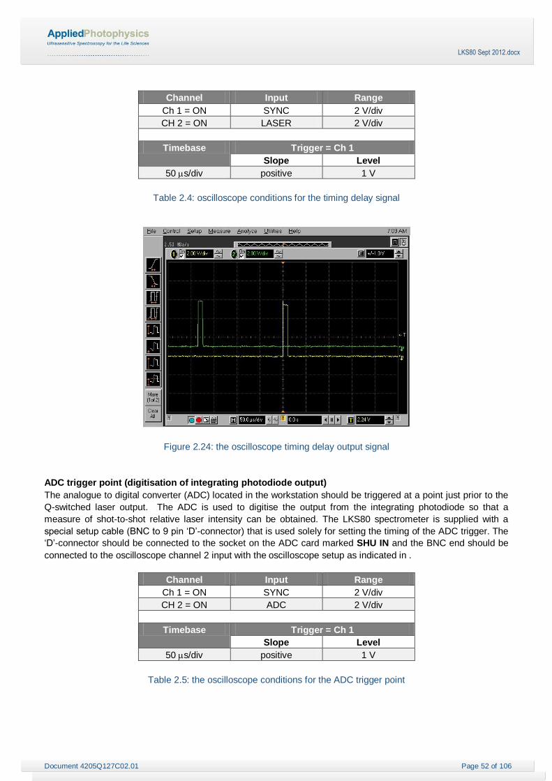
Document 4205Q127C02.01 Page 52 of 106
LKS80 Sept 2012.docx
Channel Input Range
Ch 1 = ON SYNC 2 V/div
CH 2 = ON LASER 2 V/div
Timebase Trigger = Ch 1
Slope Level
50 s/div positive 1 V
Table 2.4: oscilloscope conditions for the timing delay signal
Figure 2.24: the oscilloscope timing delay output signal
ADC trigger point (digitisation of integrating photodiode output)
The analogue to digital converter (ADC) located in the workstation should be triggered at a point just prior to the
Q-switched laser output. The ADC is used to digitise the output from the integrating photodiode so that a
measure of shot-to-shot relative laser intensity can be obtained. The LKS80 spectrometer is supplied with a
special setup cable (BNC to 9 pin ‘D’-connector) that is used solely for setting the timing of the ADC trigger. The
‘D’-connector should be connected to the socket on the ADC card marked SHU IN and the BNC end should be
connected to the oscilloscope channel 2 input with the oscilloscope setup as indicated in .
Channel Input Range
Ch 1 = ON SYNC 2 V/div
CH 2 = ON ADC 2 V/div
Timebase Trigger = Ch 1
Slope Level
50 s/div positive 1 V
Table 2.5: the oscilloscope conditions for the ADC trigger point

Document 4205Q127C02.01 Page 53 of 106
LKS80 Sept 2012.docx
The timing delay can be adjusted using the middle set of timing switches i.e. SW5 to SW8 (Section 2.11.9). SW8
changes the timing in 2.5 µs steps and SW7 changes the timing in 25 µs steps etc. The ADC switching should be
set to take place about 10 µs before the SYNC pulse occurs.
Figure 2.25:the oscilloscope ADC trigger point signal
When the spectrometer control unit is used with the Continuum Surelite Nd:YAG laser, there is a
circuit addition within the spectrometer control unit which changes the LASER and SYNC output
pulses. In this case, the quiescent state is +5 V at these output sockets (instead of 0 V) and the
LASER and SYNC output pulses bring the level down from +5 V to 0 V for the duration of the
pulses. When using the oscilloscope to view these pulses, the trigger slope should be set to
negative instead of positive.
Timing setup for the LASER output relative to the pulsed light signal
1. The following protocol uses the photomultiplier output signal and will allow the instrument timing to be set
up closer to that which will be required in normal operation. This procedure does not require that the
laser to be active as it use the SYNC output pulse from the spectrometer control unit to trigger the
oscilloscope.
2. Switch on the xenon light source.
3. Check that the PULSE output from the spectrometer controller is connected to the EXT TRIGGER input
of the arc lamp pulser.
4. Connect the SYNC output socket from the spectrometer controller to the EXTERNAL TRIGGER input of
the digitising oscilloscope. (On the Infiniium model 54830A this socket is located on the bottom right of
the front panel and is marked Aux Trig In. On the Infiniium model DSO8064A, this socket is located at
the rear of the oscilloscope.)
5. Set the LAMP DELAY control on the arc lamp pulser to 3 ms (the digit 3 showing in the window of the
control knob).
6. Set the monochromator wavelength to 450nm using the !LASER software installed on the workstation.
7. Make sure that the photomultiplier SIGNAL output is connected to the Ch1 input of the oscilloscope.
8. Using the !LASER software, set the oscilloscope time base to 2 ms/div.

Document 4205Q127C02.01 Page 54 of 106
LKS80 Sept 2012.docx
9. Apply sufficient high voltage to the detector (about 650 volts) so that the pulsed light signal has an
amplitude of 300 to 500mV (50ohm input impedance).
10. Set the arc lamp pulser PULSE ENERGY to 100 volts.
11. Check that the spectrometer controller switches are set as follows:
LAMP SHUTTER – NORMAL
LASER SHUTTER – NORMAL
EXT / INT – INT
0.1s/1s/10s – 0.1s
12. Trigger the spectrometer either by using the START switch on the spectrometer controller or by selecting
the ‘Light Level’ operation within the !LASER software. Observe the profile of the pulsed light source.
Adjust the photomultiplier high voltage if necessary and try recording the arc lamp pulse on different
timebase settings.
13. With different settings of the LAMP PULSE DELAY control on the front panel of the arc lamp pulser (i.e.
in the range 2.5 to 3.5), try repeat triggers using either the START switch or the ‘Light Level’ option in
the !LASER software. Choose an optimum setting for the LAMP PULSE DELAY control i.e. where the
beginning of the plateau region corresponds to the zero time marker on the oscilloscope display (i.e. one
horizontal division when pre-trigger is active).
Remember that the shape of the arc lamp pulse can be altered slightly by changing the position
of the tuning element which is accessed at the rear of the arc lamp pulser. There will be a
position of the tuning element that will provide optimal flatness for plateau region of the arc lamp
light pulse i.e. the region of the arc lamp pulse where transient absorption measurements will be
made.
Timing of Q-switched laser output relative to the pulsed light signal
1. The procedure in the previous section will result in timing that is very close to optimal. However,
repeating the check with the laser running is advisable.
2. Connect the LASER output at the rear of the spectrometer control unit to the flashlamp external trigger
socket on the laser power supply.
3. Connect the SYNC output at the rear of the spectrometer control unit to the Q-switch external trigger
socket on the laser power supply.
4. Connect the output from the photodiode trigger to the EXT TRIGGER input of the oscilloscope.
5. Activate the laser with the laser power supply settings set for external flashlamp trigger and external Q-
switch trigger.
6. Check that the LASER TRIGGER switch on the spectrometer controller is in the ENABLE position.
7. Trigger the spectrometer using the START switch on the spectrometer control unit or using the ‘Light
Level’ option in the !LASER software and observe the profile of the pulsed light source. Adjust the
timebase as required.
8. Adjust the LAMP PULSE DELAY control on the front panel of the arc lamp pulser until the start of the
plateau region corresponds to the zero time marker on the oscilloscope display (only a small adjustment
should be necessary).

Document 4205Q127C02.01 Page 55 of 106
LKS80 Sept 2012.docx
2.12 Trouble shooting
The LKS80 spectrometer is powered by the mains electricity supply which can produce a shock
leading to serious injury or death. Do not connect or disconnect the instrument from the mains
supply unless the supply is powered off at source. Ensure all communications and electrical
connections are made before powering on the spectrometer.
These guidelines are intended for the use of APL Service Engineers only, and the suggested actions in Table 2.6
should only be performed by the user under the direct guidance of a qualified APL Engineer. For assistance
please contact APL Technical Support Department at the address give on the front of this User Guide.
Fault Possible Causes Remedy
Arc lamp fails to
strike
Igniter spark gap has worn
(increased electrode
separation)
Arc lamp requires replacing
High voltage start pulse is
leaking to earth
A high resistance in the path
to the bottom of the lamp is
blocking the start pulse
Absence of 80 to 90 volts DC
across the lamp electrodes
(this voltage will normally
drop to 17 volts once the
lamp strikes)
Remove the igniter module from the lamp housing
support plate. Remove the cover. Identify the spark gap.
Loosen the locking nut which secures the top electrode
in the spark gap. Screw the top electrode in a clockwise
direction until it touches the bottom electrode. Now
screw the electrode in the reverse direction by ¾ of a
revolution. Tighten the locking nut, replace the cover and
remount the module on the lamp support plate.
If the lamp has been running for more than 1000 hours
then it may become more difficult to strike and should be
replaced by a new lamp following the instructions in
Section 2.11.5.
Check the way that the wiring is routed from the starter
module to the lamp housing black insulated terminal
and onwards to the bottom of the lamp. Avoid the high
voltage wire running too close to any surface that is at
ground potential.
Check whether the tag connection to the bottom of the
lamp may has become oxidised thus producing a high
resistance joint. If there is evidence of corrosion then the
connection should be taken apart and the contact
surfaces cleaned prior to reassembly. Re-solder the
connection tag if necessary.
Check that there is 80 to 90 volts between the two
horizontal pins in the Lamp Output socket at the rear of
the lamp power supply.
Check the fuse on the rear panel of the lamp power
supply.
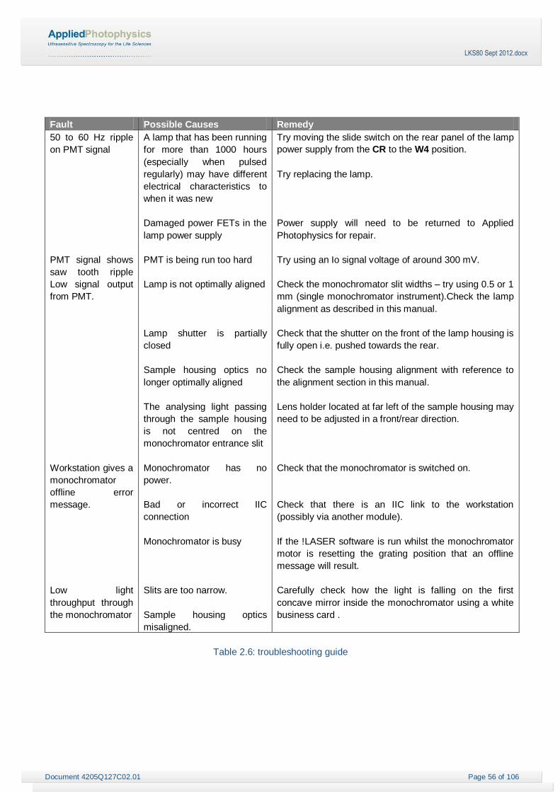
Document 4205Q127C02.01 Page 56 of 106
LKS80 Sept 2012.docx
Fault Possible Causes Remedy
50 to 60 Hz ripple
on PMT signal
PMT signal shows
saw tooth ripple
Low signal output
from PMT.
Workstation gives a
monochromator
offline error
message.
Low light
throughput through
the monochromator
A lamp that has been running
for more than 1000 hours
(especially when pulsed
regularly) may have different
electrical characteristics to
when it was new
Damaged power FETs in the
lamp power supply
PMT is being run too hard
Lamp is not optimally aligned
Lamp shutter is partially
closed
Sample housing optics no
longer optimally aligned
The analysing light passing
through the sample housing
is not centred on the
monochromator entrance slit
Monochromator has no
power.
Bad or incorrect IIC
connection
Monochromator is busy
Slits are too narrow.
Sample housing optics
misaligned.
Try moving the slide switch on the rear panel of the lamp
power supply from the CR to the W4 position.
Try replacing the lamp.
Power supply will need to be returned to Applied
Photophysics for repair.
Try using an Io signal voltage of around 300 mV.
Check the monochromator slit widths – try using 0.5 or 1
mm (single monochromator instrument).Check the lamp
alignment as described in this manual.
Check that the shutter on the front of the lamp housing is
fully open i.e. pushed towards the rear.
Check the sample housing alignment with reference to
the alignment section in this manual.
Lens holder located at far left of the sample housing may
need to be adjusted in a front/rear direction.
Check that the monochromator is switched on.
Check that there is an IIC link to the workstation
(possibly via another module).
If the !LASER software is run whilst the monochromator
motor is resetting the grating position that an offline
message will result.
Carefully check how the light is falling on the first
concave mirror inside the monochromator using a white
business card .
Table 2.6: troubleshooting guide

Document 4205Q127C02.01 Page 57 of 106
LKS80 Sept 2012.docx
2.13 Diffuse Reflectance Accessory
Figure 2.26: the diffuse reflectance accessory exterior (left) and interior (right)
The diffuse reflectance accessory (Figure 2.26) comprises two parts:
sample holder,
optical beam steering module.
These two modules are supplied mounted in a protective case for convenient and safe storage when the device
is not in use. Installation of the accessory into the sample housing requires removal of the cuvette holder
together with the second lens module (L2) used to focus the xenon light onto the standard cuvette holder. (If the
colinear arrangement had been in place then the prism module would also need to be removed from the mini
rail).
Figure 2.27: the Diffuse Reflectance Accessory mounted in the sample housing
The function of the optical module of the Diffuse Reflectance Accessory (Figure 2.28) is to redirect the incoming
xenon light beam (via two plane folding mirrors) so that it is parallel to the main optical axis. A Spectrosil lens
then focuses the optical beam onto the solid sample. The function of the second lens mounted on the optical
module is to collect diffuse reflected light and produce a converging beam which is redirected by the third folding
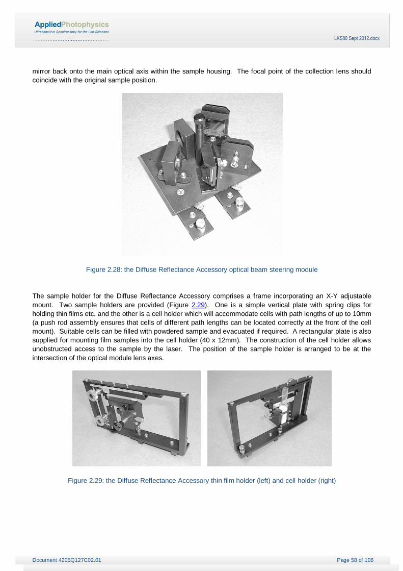
Document 4205Q127C02.01 Page 58 of 106
LKS80 Sept 2012.docx
mirror back onto the main optical axis within the sample housing. The focal point of the collection lens should
coincide with the original sample position.
Figure 2.28: the Diffuse Reflectance Accessory optical beam steering module
The sample holder for the Diffuse Reflectance Accessory comprises a frame incorporating an X-Y adjustable
mount. Two sample holders are provided (Figure 2.29). One is a simple vertical plate with spring clips for
holding thin films etc. and the other is a cell holder which will accommodate cells with path lengths of up to 10mm
(a push rod assembly ensures that cells of different path lengths can be located correctly at the front of the cell
mount). Suitable cells can be filled with powdered sample and evacuated if required. A rectangular plate is also
supplied for mounting film samples into the cell holder (40 x 12mm). The construction of the cell holder allows
unobstructed access to the sample by the laser. The position of the sample holder is arranged to be at the
intersection of the optical module lens axes.
Figure 2.29: the Diffuse Reflectance Accessory thin film holder (left) and cell holder (right)

Document 4205Q127C02.01 Page 59 of 106
LKS80 Sept 2012.docx
Although an initial alignment of the optical module is made during construction, the absolute position of the
various elements needs to be optimised for the sample housing in which the Diffuse Reflectance Accessory is to
be used. Once these adjustments have been performed for the first time, subsequent installation of the
accessory becomes a simple operation comprising mounting the accessory onto the mini optical rail and sliding it
sideways to its optimum position.
2.13.1 Initial alignment of the accessory
A schematic of the Diffuse Reflectance Accessory alignment is shown in Figure 2.30.
Figure 2.30: schematic of the Diffuse Reflectance Accessory alignment
The following instructions should be followed to set the alignment of the optical module if the module has never
previously been set up in the sample housing. However, if alignment has already been checked then no specific
adjustments should be necessary and one can proceed directly via Section 2.13.2.
1. Remove the optical module from the storage container by releasing the two captive fasteners at the
front of the module.
2. The optical elements are mounted on a support plate which has two stainless rods attached to its
underside. These are used to locate the module onto its two saddle assemblies.
3. With the xenon lamp ignited, use the spectrometer control unit to open the electrically operated shutter
located at the input port of the sample housing.
4. Inside the sample housing, undo the captive fasteners which attach the lens mount (L2) and the sample
holder to the mini rail. Lift off the lens mount and the sample holder. Note - Lens holder L2 is the
second lens in the sample holder counting from the right.
5. Move the guide plate (cross beam/colinear arrangements) to the colinear position. This will help set the
angle of the incoming laser beam.
6. Choose which sample holder is to be used with diffuse reflectance accessory (i.e. either the sample
plate or the cell holder) and attach this sample holder to the sample holder frame. (Note that these two

Document 4205Q127C02.01 Page 60 of 106
LKS80 Sept 2012.docx
holders attach to the mounting frame from opposite sides in order that the sample plane for either holder
is identical with respect to the incoming laser.)
7. Attach the sample holder frame of the Diffuse Reflectance Accessory to the mini rail using its captive
fasteners. The brass guides in the mini rail to which the sample holder frame will be attached are those
that would normally be used to fasten the prism assembly when the colinear arrangement is in use.
8. Slide the sample holder frame on the mini rail to a position (just to the right of lens holder L3) so that the
incoming laser will hit the sample..
9. Mount the optical module onto the mini rail and use a white business card to monitor the path of the
incoming xenon analysing light beam. The light beam should appear centred vertically and horizontally
on the first folding mirror. If the light beam appears to be correctly positioned in the horizontal direction
but is not at the correct height, then the optics plate can be readjusted with respect to the saddle
assemblies using the two knurled fixing screws which clamp onto the stainless steel mounting rods. If
the horizontal alignment is also incorrect then the knurled fixing screws will need to be loosened so that
the optical plate assembly can be lifted away from the saddle mounts. This will give access to the 4
fixing screws which control movement of the adjust plates attached to the saddle assemblies in a front to
rear direction (2 screws are readily accessible but 2 are located beneath the optics plate). Loosen the
four saddle plate locking screws and relocate the optics plate back into position. Adjust the height of the
optics plate to its optimum position and then tighten the knurled screws. Recheck the position of the
incoming xenon light beam on the first folding mirror and readjust the optics plate as required. Tighten
the adjust plate locking screws (only the front two will be accessible at this time).
10. The first folding mirror (DR-M1) should be directing the xenon light beam symmetrically onto the second
folding mirror. If the first folding mirror is in need of adjustment, use an M4 spanner to loosen the mount
fixing, readjust the angle of the mirror mount and relock the fixing screw. (Note - do not touch the mirror
surfaces, a disposable polythene glove is a useful aid to protect the mirrors from being touched
accidentally).
11. The second folding mirror (DR-M2) should direct the xenon light directly onto the lens holder (DR-L1). If
adjustment is required, use an M4 spanner to loosen the nut at the base of the mount. Retighten the nut
after any adjustment has been made.
12. The position of the focusing lens holder (DR-L2) is adjustable but the optimum position for the lens
holder will be as near to the sample position as the mount will allow.
13. In order to assist in alignment of the collection lens and mirror, cut a piece of white business card to a
suitable size and place at the sample position.
14. Moving the optical module to the left or to the right on the mini rail moves the point of intersection of the
probe beam axis and the collection axis relative to the sample position. The point of intersection should
be at the sample position and a white business card, placed just in front of the collection mirror (DRM3),
can be used to estimate when the diffusely reflected light that is being collected is at a maximum.
15. The angle of the collection mirror (DR-M3) on the optics module may need to be adjusted to ensure that
the diffusely reflected light is correctly directed towards the entrance slit of the monochromator.
16. In order to allow the final adjustments to be optimised, it is recommended that the cover be removed
from the monochromator.
17. Set the monochromator entrance slit to about 2 mm.
18. The diffusely reflected light from the white surface at the sample position should illuminate the central
part of the concave mirror at the rear on the right of the monochromator. A white business card should
be placed carefully just in front this mirror (Figure 2.31).

Document 4205Q127C02.01 Page 61 of 106
LKS80 Sept 2012.docx
Figure 2.31: monochromator interior with beam position optimised
19. The collection mirror (DR-M3) on the diffuse reflectance optics module should be adjusted so as to
optimise the light falling on the white business card inside the monochromator.
20. It may be necessary to iterate between two adjustments:- a) angle of collection mirror and b) to front / to
rear adjustment of the complete optics module relative to its two saddle assemblies.
21. It should not be necessary to make any adjustment to either of the sample housing lens holders L3 or
L4.
22. Once the adjustments have been optimised, the various fixing screws should be secured, business card
removed from inside the monochromator and the monochromator lid replaced.
2.13.2 Subsequent mounting of the accessory
Any future use of the accessory should not require the same degree of adjustment and only the following steps
should be necessary.
Figure 2.32: the Diffuse Reflectance Accessory mounted in position
1. Follow the procedure described in Section 2.13.1 steps 1 to 8.
2. Mount the optics module on the sample housing mini rail.
3. Sliding of the sample holder mount to a suitable position in the laser beam path and sliding the optics
module sideways relative to the sample mount to the optimum beam intersection position should be the
only two adjustments required (Section 2.13.3).
4. The signal level, as monitored on the oscilloscope, can be used to determine when the optics module is
correctly placed. Alternatively, the rear mirror on the right of the monochromator can be viewed using a

Document 4205Q127C02.01 Page 62 of 106
LKS80 Sept 2012.docx
white business card. Once there is familiarity with setting up the accessory, simply monitoring the signal
level should be all that is required to judge when the accessory is correctly positioned.
2.13.3 Adjustment of the laser beam path
Provided that the laser is a Nd:YAG, the use of a lens to focus the laser output onto the solid sample should not
be required. A cylindrical lens is recommended when using the accessory with an excimer laser which has a
rectangular beam section. Where a laser beam expander has been supplied, it is possible to mount the beam
expander, in the reverse direction, on the angled plate. In this way, a smaller diameter laser beam width will be
brought to the sample position.
The following adjustments should be undertaken with great care. If the second harmonic of a Nd:YAG laser is
being used then the laser intensity must be reduced by dropping the laser power either by reducing the charge
voltage or by stopping Q-switch operation. For the UV harmonics, Q-switching will be required. The careful use
of a white business card can be used to track the laser beam path.
1. The laser beam should be set to enter the sample housing at an oblique angle as determined by the
laser angle plate. This is done by rotating the Pellin-Broca prism beam steering module until the angle of
the laser beam path has been adjusted sufficiently (the Pellin-Broca beam steering module is located in
the laser output beam beyond the photodiode trigger/integrator module).
2. After hitting the sample, the laser will be reflected towards the front of the sample housing and the
magnetic beam dump should be attached to the front wall at a suitable position to catch the laser beam.
3. The laser shutter plate at the rear of the sample housing should be adjusted sideways so that the shutter
is centred on the laser beam path.
4. With a piece of white business card at the sample position, the sample holder frame can be adjusted
sideways on the mini rail as required and the sample holder adjusted to a suitable position using the fine
X and Y adjustments.
5. Some adjustment of the laser beam path, sample holder frame and optics module may be necessary to
ensure that the laser does not hit the collection lens holder after leaving the sample.
2.13.4 Sample position
The X, Y adjustment allows unexposed areas of sample to be moved into the laser beam after each shot if so
required. The cell holder option is useful for powdered samples. Different sized cells can be accommodated i.e.
from 10 x 2 mm to 10 x 10 mm. A 10 x 10 mm cell has the advantage of offering four sample faces for laser
measurements to be made prior to changing the sample.
Then films can be mounted either by using the 50 x 50 mm sample holder plate or by using the 40 x 12 mm plate
which can be located in the cell holder to correctly position thin films of dimensions 30 x 12 mm.
2.13.5 Choice of photomultiplier housing
For most measurements using the pulsed xenon light source, the 5-stage PMT module will be required. The 5-
stage PMT module will also be adequate for laser induced emission measurements. However, for very weak
diffuse reflectance measurements 9-stage PMT module may be required.
2.13.6 Optical filters
Inevitably there will be a significant amount of scattered laser light finding its way through the monochromator
and onto the detector. When using the 355 nm Nd:YAG third harmonic for sample excitation, the use of a glass
cut-off filter (Schott GG395) will help to reduce the amount of scattered light. The filter should be mounted in the
filter holder located between the monochromator and the sample housing.

Document 4205Q127C02.01 Page 63 of 106
LKS80 Sept 2012.docx
3 PRO-DATA LKS
3.1 Introduction
This is a reference guide; it tells you what each of the software functions does and is best used while running the
software to which it refers.
The purpose of the software is to control the spectrometer and its accessories and to acquire data. It has been
written in such a way as to be versatile enough to cope with a wide variety of experiments while being simple to
use. It operates under Windows® XP and later versions. The object-oriented modular architecture is easily
expandable, allowing the introduction of new features, anticipating future developments.
3.2 The Pro-Data LKS control window
Pro-Data LKS software is made up of several panels, where the instrument variables such as wavelength,
voltages and timings are set. The software is launched by clicking on the LKS desktop icon , and opens at
the main control window (Figure 3.1). This enables you to provide instructions to the spectrometer so that it
carries out an experiment or a series of experiments according to your requirements.
The main window is supplemented by drop-down menus for the management of files or the launching of
associated programs. Shortcuts to the most commonly used items from the drop-down menus are provided by
toolbar icons.

Document 4205Q127C02.01 Page 64 of 106
LKS80 Sept 2012.docx
Figure 3.1: the Pro-Data LKS Control Window

Document 4205Q127C02.01 Page 65 of 106
LKS80 Sept 2012.docx
3.3 The Data Acquisition panel
The Data Acquisition panel area (Figure 3.2) has a Graphical Display Area and a Task Area.
Figure 3.2: The Data Acquisition panel
3.3.1 Graphical Display Area
The Graphical Display Area is located in the left of the panel. It duplicates the digital oscilloscope display when
data is transferred from the oscilloscope to the computer. Each new trace transferred from the oscilloscope will
overlay previous traces.
3.3.2 Task Area
The Task Area is located to the right of the Graphical Display Area and contains five operation buttons and two
auxiliary buttons.
0% T Initiates the spectrometer operation which comprises pulsing the system (laser and pulsed xenon light
source) whilst keeping both the laser and analysing shutters closed so as to provide a 0% transmission baseline.
The digital oscilloscope sensitivity is automatically set according to the S1 sensitivity setting.
100% T Initiates the spectrometer operation which opens the analysing shutter, pulsing the system (laser and
pulsed xenon light source) whilst keeping the laser shutter closed so as to provide a 100% transmission
baseline. The digital oscilloscope sensitivity is automatically set according to the S1 sensitivity setting. NOTE:
The 100% transmission baseline is determined on the same sensitivity setting as the transient absorption (i.e.
Absorption see below) so that the baseline data can be subtracted from the transient data. To optimise signal
quality of the final transient data, the 100% transmission baseline is acquired with the bandwidth limit facility on
the digital oscilloscope selected.
Ems/Scat Initiates the spectrometer operation which opens the laser shutter, pulsing the system (laser and
pulsed xenon light source) whilst keeping the analysing shutter closed so as to provide a record of the scattered
light derived from the laser or laser induced luminescence from the sample. The digital oscilloscope sensitivity is
automatically set according to the S1 sensitivity setting.

Document 4205Q127C02.01 Page 66 of 106
LKS80 Sept 2012.docx
Absorption Initiates the spectrometer operation which opens both laser and analysing shutters, pulsing the
system (laser and pulsed xenon light source) so as to provide a record of a transient absorption produced within
the sample solution. The digital oscilloscope sensitivity is automatically set according to the S1 sensitivity setting.
Light Level Initiates the spectrometer operation which opens the analysing shutter, pulsing the system (laser
and pulsed xenon light source) whilst keeping the laser shutter closed so as to provide a record of the light level
over the period of the oscilloscope sweep. The digital oscilloscope sensitivity is automatically set according to the
S2 sensitivity setting. Under control from the LKS software, cursors are set up on the oscilloscope display. The
signal level between the cursors is averaged and read by the LKS software to be displayed in the Lght Level
status box. It is this value that is used as the Io value in the absorbance calculations.
Stop Stops the operations.
Pause Pauses the operations.
3.4 Connectivity panel
The Connectivity panel (Figure 3.3) indicates the connectivity (e.g. USB, LAN, GPIB) and its status to the
oscilloscope.
Figure 3.3: the Connectivity panel
Users can change the default connectivity in (preferences -> connectivity).
3.5 Laser Energy panel
The Relative Laser Energy panel (Figure 3.4) is used to display a measurement of the shot-to-shot relative
laser energy. This is derived from the digitised signal produced from the integrating photodiode that sees a small
part of the laser output. The laser is activated using the Run Laser button. A particular laser energy can be
normalised to be 100%. In addition, if an absolute measurement of the laser output energy in mJ can be
determined using a commercial laser power meter then it is possible, using the right mouse button, to toggle the
display to indicate the laser energy in mJ. The measured value for the commercial power meter can then be
entered as a calibration.
Figure 3.4: Laser Energy Panel
The BLANK button allows the integrating photodiode output to be measured in the absence of laser light. This
value will then be subtracted from future relative laser energy readings. This facility is useful should there be a

Document 4205Q127C02.01 Page 67 of 106
LKS80 Sept 2012.docx
laser energy display reading that is affected by ambient background light (i.e. operation without the laser optics
safety cover in place).
3.6 Average Shots panel
Average Shots (Figure 3.5) indicates the number of repeat shots or the number of shots used when signal
averaging is selected.
Figure 3.5: Average Shots Panel
3.7 Light Level panel
The Light Level panel (Figure 3.6) indicates the last measured Io value (i.e. analysing light intensity) displayed
in mV or, alternatively, the current value of the offset.
Figure 3.6: Light Level Panel
Set… button is used to change the offset manually. It will be enabled when Auto Offset (Experiment Setup
->Basic Settings->Auto Offset) is unselected.
3.8 Detector High Voltage panel
This panel (Figure 3.7) is used to set/get the detector high voltage (HV).
Figure 3.7: Detector High Voltage Panel
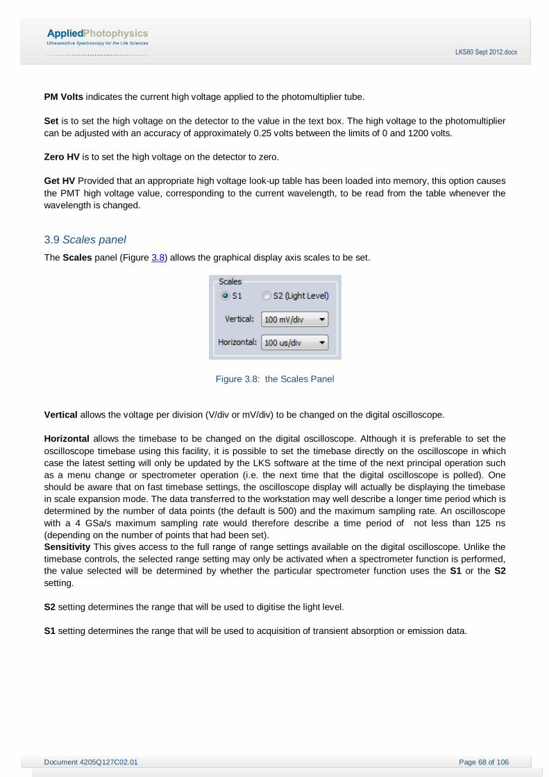
Document 4205Q127C02.01 Page 68 of 106
LKS80 Sept 2012.docx
PM Volts indicates the current high voltage applied to the photomultiplier tube.
Set is to set the high voltage on the detector to the value in the text box. The high voltage to the photomultiplier
can be adjusted with an accuracy of approximately 0.25 volts between the limits of 0 and 1200 volts.
Zero HV is to set the high voltage on the detector to zero.
Get HV Provided that an appropriate high voltage look-up table has been loaded into memory, this option causes
the PMT high voltage value, corresponding to the current wavelength, to be read from the table whenever the
wavelength is changed.
3.9 Scales panel
The Scales panel (Figure 3.8) allows the graphical display axis scales to be set.
Figure 3.8: the Scales Panel
Vertical allows the voltage per division (V/div or mV/div) to be changed on the digital oscilloscope.
Horizontal allows the timebase to be changed on the digital oscilloscope. Although it is preferable to set the
oscilloscope timebase using this facility, it is possible to set the timebase directly on the oscilloscope in which
case the latest setting will only be updated by the LKS software at the time of the next principal operation such
as a menu change or spectrometer operation (i.e. the next time that the digital oscilloscope is polled). One
should be aware that on fast timebase settings, the oscilloscope display will actually be displaying the timebase
in scale expansion mode. The data transferred to the workstation may well describe a longer time period which is
determined by the number of data points (the default is 500) and the maximum sampling rate. An oscilloscope
with a 4 GSa/s maximum sampling rate would therefore describe a time period of not less than 125 ns
(depending on the number of points that had been set).
Sensitivity This gives access to the full range of range settings available on the digital oscilloscope. Unlike the
timebase controls, the selected range setting may only be activated when a spectrometer function is performed,
the value selected will be determined by whether the particular spectrometer function uses the S1 or the S2
setting.
S2 setting determines the range that will be used to digitise the light level.
S1 setting determines the range that will be used to acquisition of transient absorption or emission data.

Document 4205Q127C02.01 Page 69 of 106
LKS80 Sept 2012.docx
3.10 Experiment Settings Front panel
This panel (Figure 3.9) duplicates some of most frequently used settings of Experiment Settings dialog box
(Section 3.15), which can be called up using the Adv… button.
Figure 3.9: Experiment Settings Front panel
3.11 Monochromator panel
Figure 3.10: Monochromator panel
The Monochromator panel of the interface (Figure 3.10) provides access to the parameters that control the
operation of the LKS monochromator. Here you set the scan range, step-size and bandwidth for your
experiment; you can also move the monochromator to a specific wavelength.
To drive the monochromator to a specific wavelength, use the Wavelength (nm) edit box and hit return on the
computer keyboard; to set the bandwidth, use the Bandwidth (nm) edit box and hit return. Setting wavelength
and bandwidth can be done simultaneously with a single return.
To set the wavelength range for a scan, use the Low and High edit boxes to set the lower and upper wavelength
limits; use the Step edit box to set the step-size; all units are nanometres. Click on the Set button or hit return to
confirm these parameters. Note that the monochromator always scans from high to low wavelength.
To save the current monochromator parameters as the default ones, click on the Adv… button, which displays
the Monochromator Wavelength Setup - Advanced panel (Figure 3.11) and click on Save As Default. Click
on OK to take you back to the Pro-Data interface.

Document 4205Q127C02.01 Page 70 of 106
LKS80 Sept 2012.docx
3.11.1 Monochromator Scan Setup: discrete wavelengths
Click the Adv… button, to open the Monochromator Wavelength Setup - Advanced dialog box (Figure 3.11).
Figure 3.11: Advanced Mono Setup
Tick the Dual mono tick box if the AM.1 option is fitted.
The first panel is the Single wavelength panel. Select Single wavelength and specify the wavelength in the
associated edit box. Click OK. The dialog box will close and the monochromator will drive to the selected
wavelength.
It is also possible to create a list of discrete wavelengths. Firstly, clear the wavelength list by clicking the Clear
list button and then select Append to list. Now select Single wavelength, specify the wavelength in the edit
box and click on Generate list. Each time you type in a wavelength and click Generate list, the specified single
wavelength will be appended to the list. When you are satisfied that the list of wavelengths is correct, click OK.
3.11.2 Monochromator Scan Setup: skip-scans
A simple wavelength range can be set in the Monochromator panel (Figure 3.10) and there is no need to use
the advanced panel to set such a range (Section 3.11). However, if you wish to carry out a more sophisticated
scan, select Wavelength range in the Monochromator Wavelength Setup - Advanced dialog box (Figure
3.11). Then clear the wavelength list by clicking the Clear list button and then select Append to list. Specify the
Start, Stop and Step values for the first wavelength range and click the Generate list button A number of
entries that correspond to your specification will appear in the list. Then enter the Start, Stop and Step values

Document 4205Q127C02.01 Page 71 of 106
LKS80 Sept 2012.docx
for the second range and click the Generate list button once more. The new values will be appended to the
existing values in the list. Repeat this cycle until you have completed the skip-scan list. The total number of
entries in the list is recorded at the foot of the list.
Skip-scans are in general used on samples that you know well and that you might wish to measure again in the
future. Use the Save As… button to save the list as a .conf (configuration) file that can be retrieved using the
Load button at a future date. This obviates the need to generate a new list every time you run the sample.
3.12 Progress and Status panel
Figure 3.12: Progress and Status Panel
The Progress and Status panel (Figure 3.12) provides information concerning the current status of the
spectrometer and of data acquisition. The box on the left of the panel will give the status (e.g. Ready,
Acquiring); the two bars to the right of the panel give a visual representation of the progress.
3.13 The Device Window
The following refers to software functionality intended for experienced users only. Changing
device parameters without a thorough knowledge of what they control may lead to undesirable
consequences.
Figure 3.13: the Device window

Document 4205Q127C02.01 Page 72 of 106
LKS80 Sept 2012.docx
Select Devices… from the View drop-down menu on the Main Control Window to reveal the Device Window
(Figure 3.13). Clicking on any of the icons shown will display a further window associated with the device,
except for the cases where access to the device window is password-protected. Access to some devices is
denied for all but trained personnel.
System Reset will reset any user-adjustable parameters accessible through the Devices window to their factory
defaults. It is unlikely that you would need to do this.
Calibrate Zero Offsets will adjust the electronic offset to take into account any small drift that may have
occurred over time. It is unlikely that you will need to this on a regular basis. The offsets should not be changed
until the instrument electronics are at their normal working temperature (it is good practice to leave the
electronics switched on at all times) nor should they be changed part-way through a series of experiments.
Service Password… opens a dialogue box that permits you to changer the password that gives access to the
advanced sections of the Devices panels. If you change it, do not forget it because APL engineers will not be
able to rediscover it for you.
3.13.1 The Main Monochromator dialog box
Clicking on the Mono 1 icon will open the Main Monochromator dialog box (Figure 3.14) .
Figure 3.14: the Main Monochromator dialog box
In the Wavelength (nm) panel, you can use the slider bar or the edit box to specify a wavelength; clicking the
Set button will drive the monochromator to the chosen wavelength. This setting is also the one to which the
monochromator will drive when the software is started. The Status panel reports what the monochromator is
doing – when it is executing your instruction, the status reported would be Updating and No respectively in the
Current action and Reached target boxes and on completion the text would read Ready and Yes.
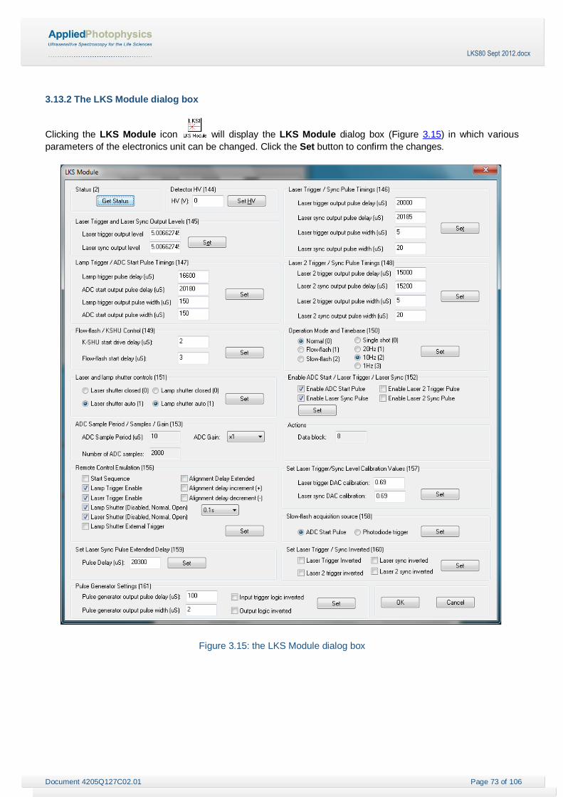
Document 4205Q127C02.01 Page 73 of 106
LKS80 Sept 2012.docx
3.13.2 The LKS Module dialog box
Clicking the LKS Module icon will display the LKS Module dialog box (Figure 3.15) in which various
parameters of the electronics unit can be changed. Click the Set button to confirm the changes.
Figure 3.15: the LKS Module dialog box

Document 4205Q127C02.01 Page 74 of 106
LKS80 Sept 2012.docx
3.14 The Preferences window
Clicking the Preferences icon from the toolbar (Section 3.16) or selecting Preferences… from the
Configuration menu (Section 3.17.3) will display the Preferences window (Figure 3.16).
3.14.1 The Connectivity tab
The Connectivity tab (Figure 3.16) enables you to specify the oscilloscope type, interface (USB, LAN, GPIB),
and address.
Figure 3.16: the Connectivity tab
3.14.2 The File Names tab
The File names tab (Figure 3.17) enables you to specify file names for absorbance and emission. In a series of
experiments, the file names will share the chosen seed name and be differentiated by an automatically
incrementing numeric component, e.g. LksAbs0001, LksAbs000.
Figure 3.17: the File Names tab

Document 4205Q127C02.01 Page 75 of 106
LKS80 Sept 2012.docx
3.14.3 The Grating Type tab
The Grating Type tab (Figure 3.18) enables you to specify the grating parameter.
Figure 3.18: the Grating Type tab
3.14.4 The Sample Delay tab
The Sample Delay tab (Figure 3.19) enables you to specify the time delay before the measurement begins.
Figure 3.19: the Sample Delay tab

Document 4205Q127C02.01 Page 76 of 106
LKS80 Sept 2012.docx
3.14.5 The Viewer tab
On the Viewer tab (Figure 3.19) you can control how the Pro-Data Viewer looks when launched (with or without
the blank display) and whether or not the display automatically rescales when a data point is measured that is
outside the limits of the currently-displayed y-axis.
Figure 3.20: the Viewer tab
3.14.6 The Startup Preferences tab
The Startup preferences tab (Figure 3.21) allows you to start the SCP in emulator mode, i.e. in the absence of
any hardware, but that is unlikely to be of interest during normal use.
Figure 3.21: the Startup Preferences tab

Document 4205Q127C02.01 Page 77 of 106
LKS80 Sept 2012.docx
3.15 The LKS Experiment Settings dialog box
Clicking on the Experiment Setup icon from toolbar or selecting Experiment Setup from the View drop-down
menu will display the LKS Experiment Settings dialog box
3.15.1 Overview window
The Overview window (Figure 3.22) shows the current status of the LKS.
Figure 3.22: the Overview window

Document 4205Q127C02.01 Page 78 of 106
LKS80 Sept 2012.docx
3.15.2 The Basic Settings dialog box
The Basic Settings dialog box (Figure 3.23) is used to set up the basic conditions for the operation of the LKS80.
Figure 3.23: the Basic Settings dialog box
Pre-Trig if this box is ticked, the data trace will show 10% pre-trigger information (i.e. the laser output will occur
one division after the start of the trace). This is the most convenient way of operating as it provides useful
baseline information immediately prior to any transient absorption. The default setting is with Pre-Trig selected.
Average if this box is ticked, multiple spectrometer operations take place according to the current Average
Shots value selected (Section 3.6). The averaged data will be displayed once the selected number of events has
been completed.
Auto Offset if this box is ticked, an automatic spectrometer sequence will be initiated whenever a 100%T or
Absorption spectrometer operation is selected so as to ensure that the signal data acquired with increasing
signal input sensitivity S1 is within the digitised range of the digital oscilloscope. The spectrometer sequence
includes a Light Level operation to determine the light level (I0 value). The numerical value of I0 is the value that
is passed to the oscilloscope for it to use as a signal offset.

Document 4205Q127C02.01 Page 79 of 106
LKS80 Sept 2012.docx
3.15.3 The Advanced Settings dialog box
The Advanced Settings dialog box (Figure 3.24) is used to set up the more complex operating conditions of the
LKS80.
Figure 3.24: the Advanced Settings dialog box
Autoscan if this box is ticked and a spectrometer operation is selected, the spectrometer will scan across the
wavelength range according to the wavelength parameters entered into the Main Monochromator dialog box
(Figure 3.14).
Autotransfer when set, signal data will be transferred automatically from the Pro-Data LKS control program to
the Pro-Data Viewer.
Set High Voltage activates an iterative routine that sets the detector high voltage to a value that produces a pre-
set detector output signal in response to the analysing light level present on the detector when the Lght Level
command is initiated. If the Setup HV table box is ticked, the operation will be performed automatically over a
number of wavelengths forming a selected wavelength range. If the Auto Set High Voltage, the operation will be
performed only at the current wavelength.
Trace position allows the trace to be optimally positioned on the oscilloscope screen.

Document 4205Q127C02.01 Page 80 of 106
LKS80 Sept 2012.docx
3.15.4 Oscilloscope Settings
The Oscilloscope Settings dialog box (Figure 3.25) is used to set the operating condition of the oscilloscope
Figure 3.25: the Oscilloscope Settings dialog box
The input channel is set using the radio buttons on the Channel in Use panel.
B/W lim - when set, the bandwidth of the digital oscilloscope signal input will be reduced from 500 MHz to 20
MHz. This is a convenient way to improve signal to noise ratio (a check must be made to ensure that there is no
observable signal distortion, particularly over short acquisition times).
50 Ohm - This option defines the input impedance of the digital oscilloscope signal input amplifier. 50 ohm is the
setting that will always be required when using very fast timebases (i.e. <100 ns/div to 50 µs/div) where
maximum bandwidth is required so as to avoid distortion of kinetic traces. For much longer timebases, the high
impedance alternative can be selected (i.e. 1 Megohm), and the variable signal terminator (set to an appropriate
value) inserted onto the signal input socket of the digital oscilloscope. When using 50 ohm termination on the
oscilloscope, the variable signal terminator must be removed from the signal input to the digital oscilloscope.
In the case of certain oscilloscopes such as the Agilent Infiniium DSO9064A, the input impedance must be kept
at 1 Megohm for absorption measurements with the 50 ohm input being provided by an inline BNC 50 ohm
terminator. This is to ensure that complete offset performance can be maintained with respect to the analysing
light signal.

Document 4205Q127C02.01 Page 81 of 106
LKS80 Sept 2012.docx
3.15.5 Remote Controller Settings
The Remote Controller Settings dialog box (Figure 3.26) is used to set the operating conditions of the remote
controller
Figure 3.26: the Remote Controller Settings dialog box
Lamp Shutter provides override control of the shutter situated in the analysing light beam allowing it to be forced
either to the open or closed positions. Only when in the Normal position will the software take control over its
opening action (the LKS software will close the shutter according to the timebase that has been set on the
oscilloscope). Additional control of the lamp shutter is proved by Trigger setup which allows closing of the lamp
shutter to be determined either by the LKS software (Ext mode) or by the spectrometer control unit plug-in card
(Int mode). When Int mode is selected, three fixed shutter opening times are available i.e. 0.1, 1.0 or 10.0
seconds.
Laser Shutter provides override control of the laser shutter allowing it to be forced either to the open or closed
positions. Only when in the Normal position will the software take control over its opening action.
Lamp Trigger controls pulsing of the xenon arc lamp (pulsing action needs to be disabled for data acquisition
periods of longer than 500 µs).
Laser Trigger controls the availability of clock pulses that are sent to the laser power supply in order to trigger
the laser flashlamp.
Laser Sync Delay provides a means whereby the delay between the trigger pulses for the laser flashlamp and
Q-switch trigger can be increased to times longer than the delay setting that is optimal for maximum laser output
energy. By increasing the delay in this way, the laser energy can be decreased.

Document 4205Q127C02.01 Page 82 of 106
LKS80 Sept 2012.docx
3.16 Toolbar Icons
The toolbar is shown in Figure 3.27. Positioning the cursor over the icon will call up a brief description of it; a
fuller description is also provided in the status bar at the foot of the interface.
Figure 3.27: Toolbar Icons
Opens a previously collected data file. This will open a window showing the contents of the currently active
directory or the examples folder if you have just launched Pro-Data. Opening a data file from this window
will configure the interface with the experimental parameters contained in that file.
Saves the active document. If there is new data that needs saving, this icon will open a Save As window
showing the currently active directory. If there is no new data, an information window saying so will
appear.
Calls up the Remarks window in which you can record information about your experiments. The remarks
are stored in the Datastore and can be viewed in Pro-Data viewer (in the lower panel of the launchpad).
Calls up the Experiment Settings window (Figure 3.9).This opens a setup wizard where you can change
the settings of the experiments (e.g. Basic Settings, Advanced Settings and Oscilloscope Settings).
Set personal preferences. This icon opens a window where you can set personal preferences (e.g. File
Names, Connectivity, Grating Type).
Launches Pro-Data Viewer, which has a separate manual. Pro-Data viewer will appear on your screen. It
will be open at the default working directory, from where you can navigate in the usual way.
Launches Laser Controller, which will appear on your screen. It will ask you to choose an available COM
port to which the laser is being connected.
Calls up About LKS window. A window will open giving the version number of the LKS software.
Launches Help. Click on the Help icon to launch the context sensitive help program. Move the cursor /
question mark to the item that you want to know about and click on it.

Document 4205Q127C02.01 Page 83 of 106
LKS80 Sept 2012.docx
3.17 Drop-down Menus
Much of what is available in the drop-down menus is more readily accessible from toolbar icons. A full list of the
functionality is given below; inevitably, there is some repetition of the information in Section 3.16.
3.17.1 File Menu
Figure 3.28: the File Menu
The File menu (Figure 3.28) is used for the usual Windows file handling operations.
3.17.2 View Menu
Figure 3.29: the View Menu
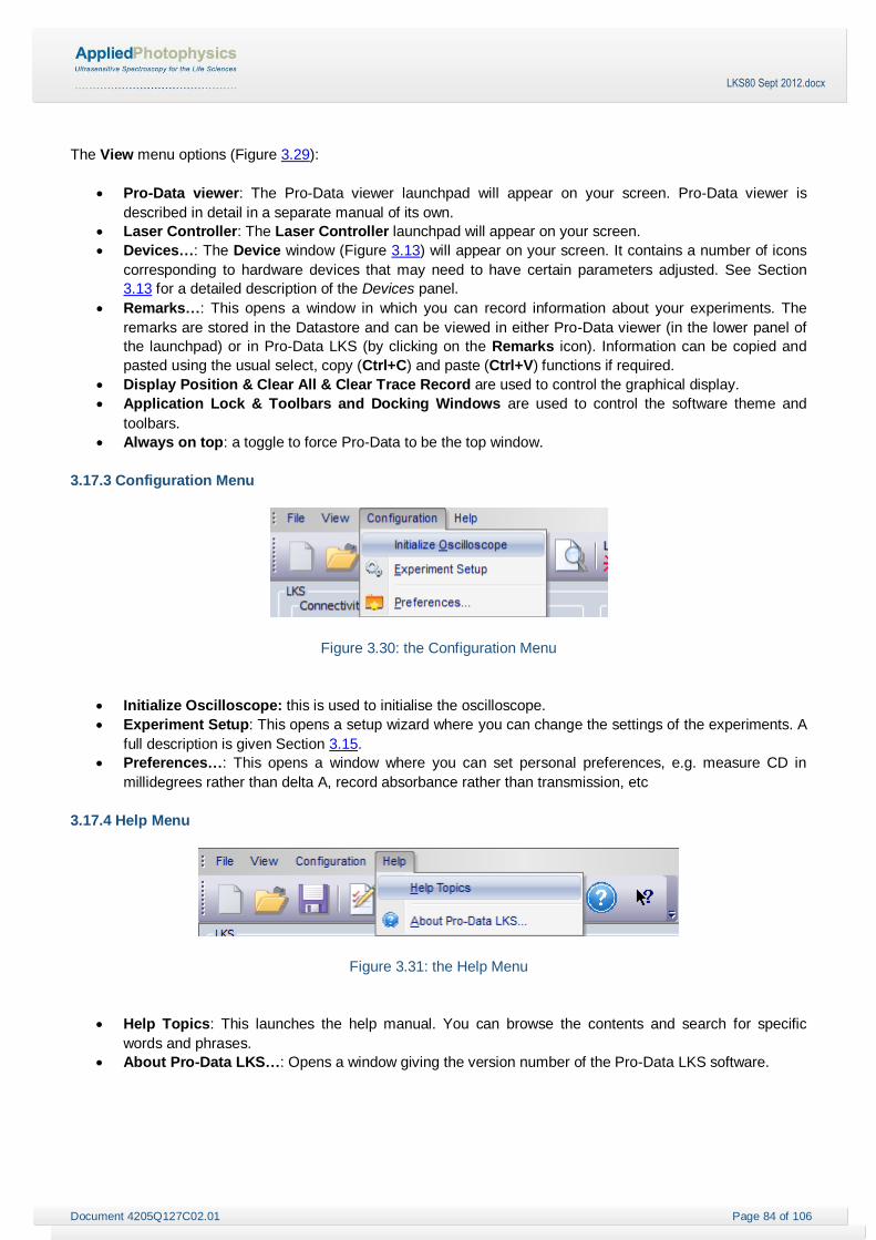
Document 4205Q127C02.01 Page 84 of 106
LKS80 Sept 2012.docx
The View menu options (Figure 3.29):
Pro-Data viewer: The Pro-Data viewer launchpad will appear on your screen. Pro-Data viewer is
described in detail in a separate manual of its own.
Laser Controller: The Laser Controller launchpad will appear on your screen.
Devices…: The Device window (Figure 3.13) will appear on your screen. It contains a number of icons
corresponding to hardware devices that may need to have certain parameters adjusted. See Section
3.13 for a detailed description of the Devices panel.
Remarks…: This opens a window in which you can record information about your experiments. The
remarks are stored in the Datastore and can be viewed in either Pro-Data viewer (in the lower panel of
the launchpad) or in Pro-Data LKS (by clicking on the Remarks icon). Information can be copied and
pasted using the usual select, copy (Ctrl+C) and paste (Ctrl+V) functions if required.
Display Position & Clear All & Clear Trace Record are used to control the graphical display.
Application Lock & Toolbars and Docking Windows are used to control the software theme and
toolbars.
Always on top: a toggle to force Pro-Data to be the top window.
3.17.3 Configuration Menu
Figure 3.30: the Configuration Menu
Initialize Oscilloscope: this is used to initialise the oscilloscope.
Experiment Setup: This opens a setup wizard where you can change the settings of the experiments. A
full description is given Section 3.15.
Preferences…: This opens a window where you can set personal preferences, e.g. measure CD in
millidegrees rather than delta A, record absorbance rather than transmission, etc
3.17.4 Help Menu
Figure 3.31: the Help Menu
Help Topics: This launches the help manual. You can browse the contents and search for specific
words and phrases.
About Pro-Data LKS…: Opens a window giving the version number of the Pro-Data LKS software.

Document 4205Q127C02.01 Page 85 of 106
LKS80 Sept 2012.docx
4 PRO-DATA VIEWER
This chapter describes the Pro-Data Viewer program, which is designed to display and manipulate data and to
store them securely.
4.1 Introduction
Pro-Data Viewer can be used either online, with a client-server link between the spectrometer control panel
(SCP) and Pro-Data Viewer, or off-line as a standalone program.
Pro-Data Viewer opens with two windows, the launchpad, which shows a list of the files in the current folder, and
the graphics display, where data will be plotted (Figure 4.1).
The status of Pro-Data Viewer is shown on the status bar at the foot of the launchpad window, where the words
Ready (Online) or Ready (Offline) will be found.
Figure 4.1: Pro-Data Viewer, showing the launchpad, left, and graphical display, right
4.1.1 Launching Pro-Data Viewer
Pro-Data Viewer can be launched as a stand-alone program using the desktop icon and will open at the
current working directory. Pro-Data Viewer will be offline when launched in this way, i.e. there will be no link with
the spectrometer control panel.
Pro-Data Viewer can also be launched from the Pro-Data LKS spectrometer control panel by clicking on the Pro-
Data Viewer launch icon in the SCP toolbar, , when a client-server link between the SCP and Pro-Data
Viewer will be established automatically. When launched in this way, Pro-Data Viewer will be online, and
becomes a live display for data as they are collected, although it can still be used for display and manipulation
purposes.
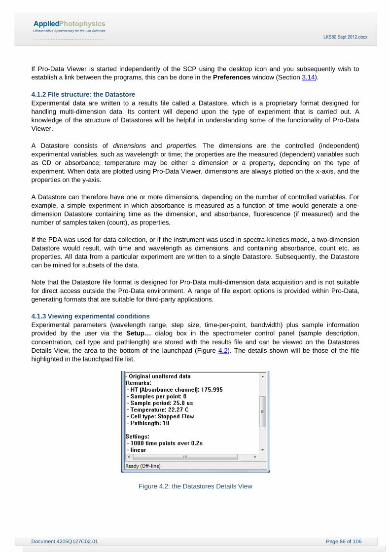
Document 4205Q127C02.01 Page 86 of 106
LKS80 Sept 2012.docx
If Pro-Data Viewer is started independently of the SCP using the desktop icon and you subsequently wish to
establish a link between the programs, this can be done in the Preferences window (Section 3.14).
4.1.2 File structure: the Datastore
Experimental data are written to a results file called a Datastore, which is a proprietary format designed for
handling multi-dimension data. Its content will depend upon the type of experiment that is carried out. A
knowledge of the structure of Datastores will be helpful in understanding some of the functionality of Pro-Data
Viewer.
A Datastore consists of dimensions and properties. The dimensions are the controlled (independent)
experimental variables, such as wavelength or time; the properties are the measured (dependent) variables such
as CD or absorbance; temperature may be either a dimension or a property, depending on the type of
experiment. When data are plotted using Pro-Data Viewer, dimensions are always plotted on the x-axis, and the
properties on the y-axis.
A Datastore can therefore have one or more dimensions, depending on the number of controlled variables. For
example, a simple experiment in which absorbance is measured as a function of time would generate a one-
dimension Datastore containing time as the dimension, and absorbance, fluorescence (if measured) and the
number of samples taken (count), as properties.
If the PDA was used for data collection, or if the instrument was used in spectra-kinetics mode, a two-dimension
Datastore would result, with time and wavelength as dimensions, and containing absorbance, count etc. as
properties. All data from a particular experiment are written to a single Datastore. Subsequently, the Datastore
can be mined for subsets of the data.
Note that the Datastore file format is designed for Pro-Data multi-dimension data acquisition and is not suitable
for direct access outside the Pro-Data environment. A range of file export options is provided within Pro-Data,
generating formats that are suitable for third-party applications.
4.1.3 Viewing experimental conditions
Experimental parameters (wavelength range, step size, time-per-point, bandwidth) plus sample information
provided by the user via the Setup… dialog box in the spectrometer control panel (sample description,
concentration, cell type and pathlength) are stored with the results file and can be viewed on the Datastores
Details View, the area to the bottom of the launchpad (Figure 4.2). The details shown will be those of the file
highlighted in the launchpad file list.
Figure 4.2: the Datastores Details View

Document 4205Q127C02.01 Page 87 of 106
LKS80 Sept 2012.docx
4.2 Displaying and selecting data
4.2.1 The graphical display
One or more files can be displayed in the graphical display
To display a single file double-click on the filename or choose Open from the File menu (Section 4.7.1).
To add a file to the graphical display, drag it onto the display or right-click and choose Add DataStore
to Graph.
To add more than one file at a time, select multiple files from the list in the usual way (using the mouse
pointer with Ctrl or Shift keys) and drag them onto the graphical display (Figure 4.3).
To display a file in a new window, double-click on the filename or choose Open from the File menu
(Section 4.7.1).
To remove a trace from the display select the trace (Section 4.2.2), right-click and choose Remove
Selected Trace or use the Trace manipulation dialog box (Section 4.3.1).
Figure 4.3: three files selected in the launchpad and dragged onto the display
4.2.2 Selecting a trace in the display
A trace can be selected in a number of ways. Once selected, it changes colour to black, is highlighted with
‘selection marks’ and cross-hairs appear on it. The value of the x- and y-coordinates at the position of the cross
hairs are shown above the graph (Figure 4.4). Single trace selection methods are listed below.
Place the mouse cursor close to the trace of interest. Left-click to select it. Click a second time to
deselect it.
Right-click anywhere in the display window to reveal a pop-up menu. Choose Select Specific Traces to
open a dialog box containing a list of the spectra displayed. Click on a filename to select it and OK to
close the dialog box.
On the Trace menu click Selection Dialog to open the Trace Manipulation dialog box (Section 4.3.1).
Click on a filename to select it and OK to close the dialog box.From the toolbar, click on the icon to
open the Selection dialog box. Click on a filename to select it and OK to close the dialog box.

Document 4205Q127C02.01 Page 88 of 106
LKS80 Sept 2012.docx
Figure 4.4: five traces displayed with one trace selected
The method of selection will depend on personal preference and on the number of traces displayed. For
example, if you wish to select one trace from several overlapping traces, using the dialog is easier than using the
mouse pointer. Once a trace is selected, the Up / Down arrow keys can be used to move the selection
sequentially through the displayed traces.
4.2.3 Selecting more than one trace
Selecting more than one trace is often required, for example to average several traces. Variations in the methods
described in the Section 4.2.2 to select a single trace are used to select more than one.
When using the mouse pointer to select spectra, hold down the Shift key and click on the spectra of
interest. Clicking on the same trace twice with the Shift key depressed will first select it and then
deselect it.
When selecting from the drop-down list, hold down the Shift key and click on the filenames of interest.
Clicking on the same filename twice with the Shift key depressed will first select it and then deselect it.
When selecting from the Trace manipulation dialog box (Section 4.3.1), use the Ctrl and Shift keys in
combination with the mouse to select filenames in the usual way. Selected files are highlighted. In
general, using the dialog box is the preferred method when dealing with more than one trace.
4.2.4 Zooming and re-scaling the display using the mouse
To zoom in to a particular part of the display, click and hold the left mouse button while moving the pointer to
create a box around the area of interest. On releasing the left mouse button, the newly created box will expand to
fill the display window (Figure 4.5). To return to full display, double-click in the display area.

Document 4205Q127C02.01 Page 89 of 106
LKS80 Sept 2012.docx
Figure 4.5: full display (left) and zoom using the left mouse button (right)
Use the mouse wheel to expand or contract both axes simultaneously. Hold down the Ctrl key and use the
mouse wheel to expand or contract only the horizontal axis. Hold down the Shift key and use the mouse wheel
to expand or contract only the vertical axis (Figure 4.5).
Figure 4.6: zoom using wheel alone (left), Ctrl + wheel (centre),
Shift + wheel (right)
The zoom functions can be used in any combination. To return to the default full-screen display, doublet-click at
any time in the display area.
4.2.5 Displaying different properties
Pro-Data Viewer always plots the dimension on the x-axis, and the selected property on the y-axis. Right-clicking
the y-axis legend will display a menu of the properties recorded during a measurement (Figure 4.7). To change
the property displayed, select one from the list by double-clicking it.
Figure 4.7: example menu of properties that can be plotted as y-axis

Document 4205Q127C02.01 Page 90 of 106
LKS80 Sept 2012.docx
When run in absorbance mode, three properties are recorded with every measurement made on the LKS80.
These are:
Transmission
Absorbance
Count (the number of 25 s samples taken at each step in the scan)
In addition, Fluorescence can be plotted if it was selected and a fluorescence detector was fitted.
4.3 Manipulating and Fitting Data
4.3.1 Trace Manipulation
The Trace Manipulation dialog box (Figure 4.8) can be opened by clicking Selection dialog on the Trace menu
(Section 4.8.3) or by clicking on the graphical display toolbar (Section 4.6.2).
The dialog box is an environment in which data (traces) can be background corrected, averaged or otherwise
manipulated. All operations carried out within this environment are reversible, which means that if errors are
made they can be quickly and easily corrected. The original data are never over-written or otherwise destroyed
and all operations carried out on data are recorded in the History file on the View menu (Section 4.7.2). The
results of the manipulations are displayed in real-time and can be saved at the end of the session in one of a
number of formats using Save current plot on the File menu (Section 4.7.1).
Figure 4.8: the Trace Manipulation dialog box
The structure of the dialog box is straightforward. There are two windows, one of which lists any traces that are
visible in the graphics window, the other listing those that have been removed from the display during the
session and are no longer shown in the display. The buttons on the right execute actions on traces that have
been highlighted in the Visible Traces window. Traces can be swapped between the Removed Traces and
Visible Traces window using the arrow buttons between the two panes. Single arrow will move a selection,
double arrow will move all listed traces.

Document 4205Q127C02.01 Page 91 of 106
LKS80 Sept 2012.docx
In the example below, there are five traces, named Run1 to Run 5. We will average the first three traces, and
smooth the averaged curve. With the data loaded into the display as previously described, and the graphical
display active, open the dialog box to display the data files list (Figure 4.9).
Figure 4.9: raw data with dialog box called up
Select the files for averaging and click Average. A file named Average: 0 will be added to the Visible Traces list
and plotted in the display.
Select the Average: 0 file and click Smooth. The Smoothing dialog box will appear (Figure 4.10).
Figure 4.10: An appropriate smooth (left) and an inappropriate one (right)
Enter the number of degrees of smoothing required in the Window Size box. This value will depend on the step
resolution used during the measurement and the sharpness of the features in the trace. The number should be
as large as is possible without causing distortion of the trace. Examination of the residual plot will show if any
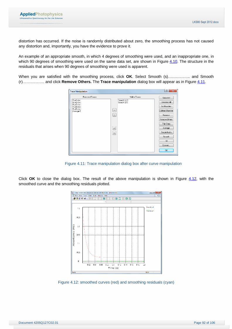
Document 4205Q127C02.01 Page 92 of 106
LKS80 Sept 2012.docx
distortion has occurred. If the noise is randomly distributed about zero, the smoothing process has not caused
any distortion and, importantly, you have the evidence to prove it.
An example of an appropriate smooth, in which 4 degrees of smoothing were used, and an inappropriate one, in
which 90 degrees of smoothing were used on the same data set, are shown in Figure 4.10. The structure in the
residuals that arises when 90 degrees of smoothing were used is apparent.
When you are satisfied with the smoothing process, click OK. Select Smooth (s)…………….. and Smooth
(r)…………….. and click Remove Others. The Trace manipulation dialog box will appear as in Figure 4.11.
Figure 4.11: Trace manipulation dialog box after curve manipulation
Click OK to close the dialog box. The result of the above manipulation is shown in Figure 4.12, with the
smoothed curve and the smoothing residuals plotted.
Figure 4.12: smoothed curves (red) and smoothing residuals (cyan)

Document 4205Q127C02.01 Page 93 of 106
LKS80 Sept 2012.docx
Note that even after closing the Trace Manipulation dialog box, any removed traces are remembered. Should
you wish to carry out further manipulation, simply re-open the dialog box and all the traces will be listed, whether
visible or removed, enabling you to carry on where you left off.
4.3.2 Curve Fitting
Select the curve you want to fit and open the Curve Fitting dialog box (Figure 4.13) using by choosing Fitting
on the Math menu (Section 4.8.4), on the graphical display toolbar (Section 4.6.2), or the Fit button on the
Trace Manipulation dialog box (Section 4.3.1).
A selected function is fitted to the data using a Marquardt-Levenberg algorithm. Select the required function from
the dropdown list on the Fitting panel and enter the range over which the data are to be fitted on the Fit Range
panel, then click Set to update. If you are unsure about initial starting parameters for the fit, click the Estimate
button to automatically generate a set of initial parameters, which may not be very accurate. The curve
associated with these parameters is plotted in the preview window to the right.
Figure 4.13: kinetic data fitted with a single exponential model
To initiate the fitting of the parameters to the data, click Fit. The algorithm will iterate until convergence or the
maximum number of cycles is reached. If the fitting is successful, the parameters will be updated and the
calculated curve plotted in the preview window. The associated residual trace (the difference between the
observed and calculated data) will be displayed in the Residuals part of the preview window. The errors
associated with the calculated parameters are displayed next to the calculated parameters. You will be able to
judge the quality of the fit by inspecting the residual trace and the parameter errors. If the errors are large
compared with the parameters, then it is likely that you have specified a fitting function which is more
complicated than is justified by the data, i.e. the result is under-determined. The number of variable parameters

Document 4205Q127C02.01 Page 94 of 106
LKS80 Sept 2012.docx
can be reduced by locking any parameter using the check boxes adjacent to the parameters, but such locking
must be justified and should be applied with care.
If the fitting process does not converge within the selected maximum number of iterations, a warning is given.
You may wish to increase the number of iterations, up to a maximum of 1000. Be aware that 1000 iterations of
the fitting algorithm may take some time. In some instances, the fitting does not converge because of the
absence of a unique solution. This too is symptomatic of an under-determined model.
When you are satisfied that the fit is a good one and the calculated parameters are sensible, you can print out a
report by clicking on the printer icon. The report displays the data, the calculated fit data with residuals and the
associated fitting parameters.
To plot the fitted curve in the Pro-Data Viewer display, click OK. If you do not wish the residuals to be included
on the plot, clear the Include Residuals in Final Plot check box.
4.3.3 Saving data
The manipulated data are not saved automatically. To save the result, go to Save Current Plot… on the File
menu (Section 4.7.1) to call up the Save As… dialog box or Save selected traces on the File menu. The
original raw data are never over-written. The results of any manipulation are stored in a new Datastore and a
complete history of the manipulated traces is contained in the History of that Datastore which is opened on the
View menu (Section 4.7.2).
4.4 Exporting data
Right-click on a filename in Pro-Data viewer launchpad to display the File manipulation pop-up menu shown in
Figure 4.14.
Figure 4.14: File manipulation pop-up menu
Select Export data… to bring up the dropdown list in Figure 4.15 and choose an appropriate format for export to
another program

Document 4205Q127C02.01 Page 95 of 106
LKS80 Sept 2012.docx
Figure 4.15: options for exporting data
CSV format is suitable for third-party programs such as Microsoft Excel; other options relate to formats derived
from other APL products.
4.5 Handling multi-dimension Datastores
4.5.1 Loading multi-dimension Datastores
In the example that follows, the PDA was used to monitor the acid catalysed redox reaction (Figure 4.16). The
PDA measures absorbance as a function of wavelength for a set period of time, so absorbance is the only
property in this case, and wavelength and time are the two dimensions.
Figure 4.16: PDA data plotted with wavelength as the x-axis
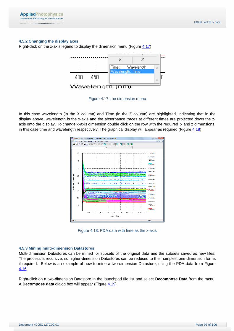
Document 4205Q127C02.01 Page 96 of 106
LKS80 Sept 2012.docx
4.5.2 Changing the display axes
Right-click on the x-axis legend to display the dimension menu (Figure 4.17)
Figure 4.17: the dimension menu
In this case wavelength (in the X column) and Time (in the Z column) are highlighted, indicating that in the
display above, wavelength is the x-axis and the absorbance traces at different times are projected down the z-
axis onto the display. To change x-axis dimension double click on the row with the required x and z dimensions,
in this case time and wavelength respectively. The graphical display will appear as required (Figure 4.18)
Figure 4.18: PDA data with time as the x-axis
4.5.3 Mining multi-dimension Datastores
Multi-dimension Datastores can be mined for subsets of the original data and the subsets saved as new files.
The process is recursive, so higher-dimension Datastores can be reduced to their simplest one-dimension forms
if required. Below is an example of how to mine a two-dimension Datastore, using the PDA data from Figure
4.16.
Right-click on a two-dimension Datastore in the launchpad file list and select Decompose Data from the menu.
A Decompose data dialog box will appear (Figure 4.19).
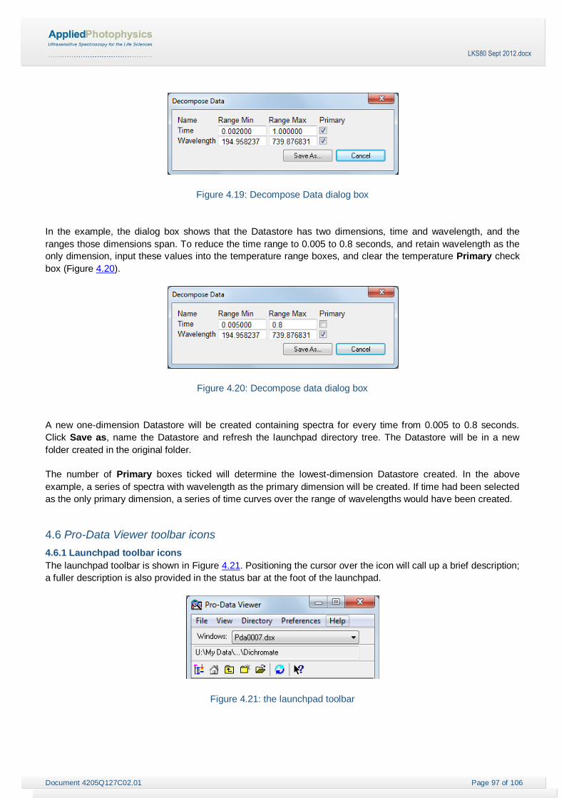
Document 4205Q127C02.01 Page 97 of 106
LKS80 Sept 2012.docx
Figure 4.19: Decompose Data dialog box
In the example, the dialog box shows that the Datastore has two dimensions, time and wavelength, and the
ranges those dimensions span. To reduce the time range to 0.005 to 0.8 seconds, and retain wavelength as the
only dimension, input these values into the temperature range boxes, and clear the temperature Primary check
box (Figure 4.20).
Figure 4.20: Decompose data dialog box
A new one-dimension Datastore will be created containing spectra for every time from 0.005 to 0.8 seconds.
Click Save as, name the Datastore and refresh the launchpad directory tree. The Datastore will be in a new
folder created in the original folder.
The number of Primary boxes ticked will determine the lowest-dimension Datastore created. In the above
example, a series of spectra with wavelength as the primary dimension will be created. If time had been selected
as the only primary dimension, a series of time curves over the range of wavelengths would have been created.
4.6 Pro-Data Viewer toolbar icons
4.6.1 Launchpad toolbar icons
The launchpad toolbar is shown in Figure 4.21. Positioning the cursor over the icon will call up a brief description;
a fuller description is also provided in the status bar at the foot of the launchpad.
Figure 4.21: the launchpad toolbar

Document 4205Q127C02.01 Page 98 of 106
LKS80 Sept 2012.docx
Defines the currently selected directory (folder) as the working directory i.e. the directory in which any
new data files will be stored. The current working directory is always shown in the box immediately
above the toolbar icons. The directory name will sometimes need to be contracted to fit in the box but the
first and last part of the name are always shown.
Returns you to the current working directory
Moves the working directory up one level, to enable you to access files in directories higher up the tree.
Creates a new folder in the currently selected directory.
Opens a browser window from which you can navigate quickly and easily to other folders.
Refreshes the directory tree display. This should be done after saving a file following averaging or
smoothing, for example, as the live directory is not automatically updated.
Click this icon and then on item of interest to call up the context sensitive help for that item.
4.6.2 Graphical display toolbar icons
The graphical display toolbar is shown in Figure 4.22.
Figure 4.22: the Standard toolbar
Saves all the traces in the display into a new file. Click on this icon to call up the Save As… dialog box
from where you can specify a filename and choose a location for the new file.
Prints the active document.
Causes an edit box to appear enabling you to record information in addition to that recorded
automatically or entered through the Setup… dialogue box in the SCP.
Calls up a history of the operations performed on the trace.
Print the active document.
Sets a selected trace as a background. Clicking again will reset the trace to its original status.
Adds a previously defined background to a selected trace or traces. It is useful if a background has been
subtracted inadvertently from a trace. This icon is inactive if no background has been defined.
Subtracts a previously defined background from a selected trace. This icon is inactive if no background
has been defined.

Document 4205Q127C02.01 Page 99 of 106
LKS80 Sept 2012.docx
Opens the Curve fitting dialog box enabling one of a number of models to be fitted to a selected trace
(Section 4.3.2).
Averages the selected traces: the average will be added to the plot.
Averages all the traces in the display, plots the average, and removes the original data.
Opens the Simple math dialog box that enables you to add, subtract, multiply or divide a trace to, from
or by a constant.
Opens the Smoothing dialog box enabling a reversible Savitsky-Golay smoothing operation to be
performed on a selected trace. The smoothed trace and (optionally) its residual are plotted (Section 4.3).
Opens the Convert CD units dialog box enabling you to convert from the current CD units to others
(This icon is greyed out for SX data).
Opens the Trace Manipulation dialog box (Section 4.3.1)
Opens the Visible Trace Range dialog box to reduce the number of traces from the same Datastore that
are displayed.
Removes all overlaid traces from the display. An overlaid trace is one whose property and dimension
(e.g. CD and wavelength) are the same as those of traces already in the display but whose wavelength
range or step-size or bandwidth differs from the originals.
Changes the x-axis to logarithmic scale. Clicking again on the icon will change the axis back to a linear
scale. A logarithmic scale is mainly used when time is plotted as the x-axis.
Resets the trace colours to the first available in the palette. This can be useful after trace manipulation if
the automatically assigned colours are not suitable, e.g. too pale.
4.7 Launchpad drop-down menus
4.7.1 The File menu
Figure 4.23: the File menu
The File menu (Figure 4.23) presents the usual Windows options for opening and closing files.

Document 4205Q127C02.01 Page 100 of 106
LKS80 Sept 2012.docx
4.7.2 The View menu
Figure 4.24: the View menu
On the View menu (Figure 4.24)
Close all viewer windows is a quick means of closing all Pro-Data Viewer graphical displays. It is
useful if Single Window in the Preferences drop-down menu has not been selected.
Always on top is a toggle to force Pro-Data Viewer to be the top window.
4.7.3 The Directory menu
Figure 4.25: the Directory menu
The Directory menu (Figure 4.25) can be used to set the current working directory or to return to it.
Move Root Directory Up One Level will take you back through the directory tree one node at a time
Set working directory will define the currently selected directory (folder) as the working directory
Back to working directory will take you directly back to the current working directory
New folder will create a new folder in the currently selected directory.
Browse for folders allows you to browse easily to a folder that can then be set as the working folder

Document 4205Q127C02.01 Page 101 of 106
LKS80 Sept 2012.docx
4.7.4 The Preferences menu
Figure 4.26: the Preferences menu
The Preferences menu (Figure 4.26) is used to set the conditions for the graphics display and on-line status.
Single Window when selected means that whenever a new graphical display is opened during data
acquisition, all previous ones are closed. If it is not selected, then whenever a new measurement is
made, the previous displays are not closed, but will remain open on separate tabs; If you are running an
experiment that involves a lot of repeat measurements, it is recommended that Single Window be
selected; if not, you could end up with a large number of displays to close. Single Window has no effect
when opening files from the launchpad.
Show Online Plots on the Same View will plot the acquired data on the active window.
The online status is set by clicking Go on-line, which will display the Connect dialog box (Figure 4.27)
on which you will be asked to supply the LKS IP Address. It is used when Pro-Data Viewer has been
started as a stand-alone program and you want subsequently to establish a link with the spectrometer
control program (SCP). If the two programs are running on the same computer, select Local in the
Connect window. The IP address under these circumstances is always the default 127.0.0.1.
Figure 4.27: the Connect dialog box
The client-server architecture permits remote monitoring of experiments in progress. If a copy of Pro-Data Viewer
is installed on a remote computer, establishing a client-server link established using the Remote setting will
enable you to follow an experiment on the second computer.
The IP address of the LKS computer will not be the same as the default local IP address – your network
administrator will be able to inform you. If the address is correct and the instrument is running, the Pro-Data

Document 4205Q127C02.01 Page 102 of 106
LKS80 Sept 2012.docx
Viewer display panel will open. Pro-Data Viewer will ‘listen’ to LKS and report its status, behaving as a real-time
display. If the address in incorrect, the error message shown in Figure 4.28 will appear.
Figure 4.28: the Connection error message
4.7.5 The Help menu
Figure 4.29: the Help menu
The Help menu (Figure 4.29) gives access to the Pro-Data Viewer launchpad help system
4.8 Graphical Display drop down menus
4.8.1 The File menu
Figure 4.30: the File menu

Document 4205Q127C02.01 Page 103 of 106
LKS80 Sept 2012.docx
The File menu (Figure 4.23) allows the Current plot to be saved, or the selected traces. The plot can be copied to
the clipboard or printed directly.
4.8.2 The View menu
Figure 4.31: the View menu
On the View menu (Figure 4.24):
Aux Dimension Ctrl is a toggle to show or hide the third dimension slider bar. It is of use when dealing
with multi-dimension Datastores
Legend is a toggle to hide or show the trace names that appear by default at the side of a plot. The
function can be more easily executed using the keyboard shortcut L or by right-clicking anywhere in the
plot border and clicking on the Hide legend or Show legend pop-up that appears.
Remarks… calls up an edit box in which you can add comments to supplement information that is
recorded automatically or entered through the Setup… dialogue box in the SCP.
4.8.3 The Trace menu
Figure 4.32: the Trace menu
On the Trace menu (Figure 4.32):
Show Trace Name is a toggle to show / hide the name of a highlighted trace when the mouse pointer is
placed near to it.

Document 4205Q127C02.01 Page 104 of 106
LKS80 Sept 2012.docx
Selection Dialog calls up the Trace Manipulation dialog box (Section 4.3.1).
Select All selects every trace in the display.
Deselect All deselects every trace in the display.
Remove Selected removes from the display any currently selected trace. Removed traces can be
recovered using the Trace Manipulation dialog box (Section 4.3.1).
Remove Unselected Traces removes from the display any trace that is not selected. Removed traces
can be recovered using the Trace Manipulation dialog box (Section 4.3.1).
Toggle Selected as Baseline sets / unsets a selected trace as a baseline.
Add Baseline and Subtract Baseline become active once a baseline has been set and respectively
add a baseline to a selected trace or subtract a baseline from it.
Remove Overlaid Traces removes all overlaid traces. An overlaid trace is one whose property and
dimension (e.g. CD and wavelength) are compatible with those of traces already in the display but
whose wavelength range or step-size or bandwidth is incompatible with those traces already in the
display. Overlaid traces cannot be manipulated and are always coloured black to differentiate them from
active traces.
Recompute Trace Colours will assign new colours to the traces in the display. This is useful if after
manipulation the colours of the traces are not satisfactory.
Reset will undo all operations carried out on the original data and restore the original display.
4.8.4 The Math menu
Figure 4.33: the Math menu
All mathematical functions can be called up using keyboard shortcuts or toolbar icons.
Fitting… calls up the Curve fitting dialog box .
Average calculates and plots the average of the selected traces.
Average All Traces calculates and plots the average of all the traces in the display. The original traces
are removed. Removed traces can be recovered using the Trace Manipulation dialog box (Section
4.3.1).
Simple Math… opens a dialog box that enables you to add or subtract a constant to a trace or multiply
or divide a trace by a constant. It can be useful for offsetting one trace from another for display purposes
or for normalizing spectra for easier comparison.
Smooth… opens a window for applying a smoothing algorithm to raw data. It allows you to optimize the
smoothing before accepting it.
For more information on the Fitting and Smooth functions, see Section Figure 4.3.

Document 4205Q127C02.01 Page 105 of 106
LKS80 Sept 2012.docx
4.8.5 The Scale menu
Figure 4.34: the Scale menu
On the Scale menu (Figure 4.34):
Set Plot limits… calls up a dialog box that enables you to set the limits for the x- and y-axes.
Reset Zoom resets the scale to the original display size. Double left-clicking anywhere in display window
will achieve the same thing.
X Logarithmic will change the x-axis to a logarithmic scale. This feature can be useful for kinetic data.
4.8.6 The Window menu
Figure 4.35: the Window menu
On the Window menu (Figure 4.35):
New Window… up a list from which can be selected the desired property. The new window will be
displayed at the same time as the original window in a tile format.
Close will close the currently active window
Cascade will display in a cascade format all property windows (e.g. CD, absorbance, HT) that have
been opened and are not currently minimized.
Tile will display in a tiled format all property windows (e.g. CD, absorbance, HT) that have been opened
and are not currently minimized.
Arrange icons will tidy up any minimized property displays that have been strewn around the display
window.
Close All Documents will close all the currently active windows.
1, 2 etc. refer to the open windows: the displayed window is identified by the icon
Windows… opens a dialog box that enables you to activate or close displays selected from a list.
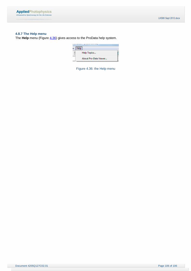
Document 4205Q127C02.01 Page 106 of 106
LKS80 Sept 2012.docx
4.8.7 The Help menu
The Help menu (Figure 4.36) gives access to the ProData help system.
Figure 4.36: the Help menu